DASAR TRANSFORMASI LAPLACE - Universitas Brawijaya · (2) The transform of an expression that is multiplied by a constant is the constant multiplied by the transform. That is: ^ `

Matematika Industri II

DASAR TRANSFORMASI

LAPLACE



Bahasan

• Transformasi Laplace

• Transformasi Laplace Invers

• Tabel Transformasi Laplace

• Transformasi Lplace dari Suatu Turunan

• Dua Sifat Transformasi Laplace

• Membuat Transformasi Baru

• Transformasi Laplace dari Turunan yang Lebih Tinggi


Bahasan









Transformasi Laplace

• A differential equation involving an unknown function f ( t ) and its derivatives is said to be initial-valued if the values f ( t ) and its derivatives are given for t = 0. these initial values are used to evaluate the integration constants that appear in the solution to the differential equation.

• The Laplace transform is employed to solve certain initial-valued differential equations. The method uses algebra rather than the calculus and incorporates the values of the integration constants from the beginning.


Introduction to Laplace transforms

The Laplace transform

Given a function f ( t ) defined for values of the variable t > 0 then the Laplace

transform of f ( t ), denoted by:

is defined to be:

Where s is a variable whose values are chosen so as to ensure that the semi-

infinite integral converges.

( )L f t

0

( ) ( )st

t

L f t e f t dt



The Laplace transform

For example the Laplace transform of f ( t ) = 2 for t ≥ 0 is:

0

0

0

( ) ( )

2

2

2(0 ( 1/ ))

2 provided > 0

st

t

st

t

st

t

L f t e f t dt

e dt

e

s

s

ss


Bahasan










The inverse Laplace transform

The Laplace transform is an expression involving variable s and can be

denoted as such by F (s). That is:

It is said that f (t) and F (s) form a transform pair.

This means that if F (s) is the Laplace transform of f (t) then f (t) is the inverse

Laplace transform of F (s).

That is:

( ) ( )F s L f t

1( ) ( )f t L F s



The inverse Laplace transform

For example, if f (t) = 4 then:

So, if:

Then the inverse Laplace transform of F (s) is:

4( )F s

s

1 ( ) ( ) 4L F s f t

4( )F s

s


Bahasan










Table of Laplace transforms

To assist in the process of finding Laplace transforms and their inverses a table

is used. For example:

1

2

( ) { ( )} ( ) { ( )}

0

1

1

( )

kt

kt

f t L F s F s L f t

kk s

s

e s ks k

te s ks k


Bahasan




• Transformasi Laplace dari Suatu Turunan






Laplace transform of a derivative

Given some expression f (t) and its Laplace transform F (s) where:

then:

That is:

0

( ) ( ) ( )st

t

F s L f t e f t dt

0

00

( ) ( )

( ) ( )

(0 (0)) ( )

st

t

st st

tt

L f t e f t dt

e f t s e f t dt

f sF s

( ) ( ) (0)L f t sF s f


Bahasan




• Transformasi Laplace dari Suatu Turunan






Two properties of Laplace transforms

The Laplace transform and its inverse are linear transforms. That is:

(1) The transform of a sum (or difference) of expressions is the sum (or

difference) of the transforms. That is:

(2) The transform of an expression that is multiplied by a constant is the

constant multiplied by the transform. That is:

1 1 1

( ) ( ) ( ) ( )

( ) ( ) ( ) ( )

L f t g t L f t L g t

L F s G s L F s L G s

1 1( ) ( ) and ( ) ( )L kf t kL f t L kF s kL F s




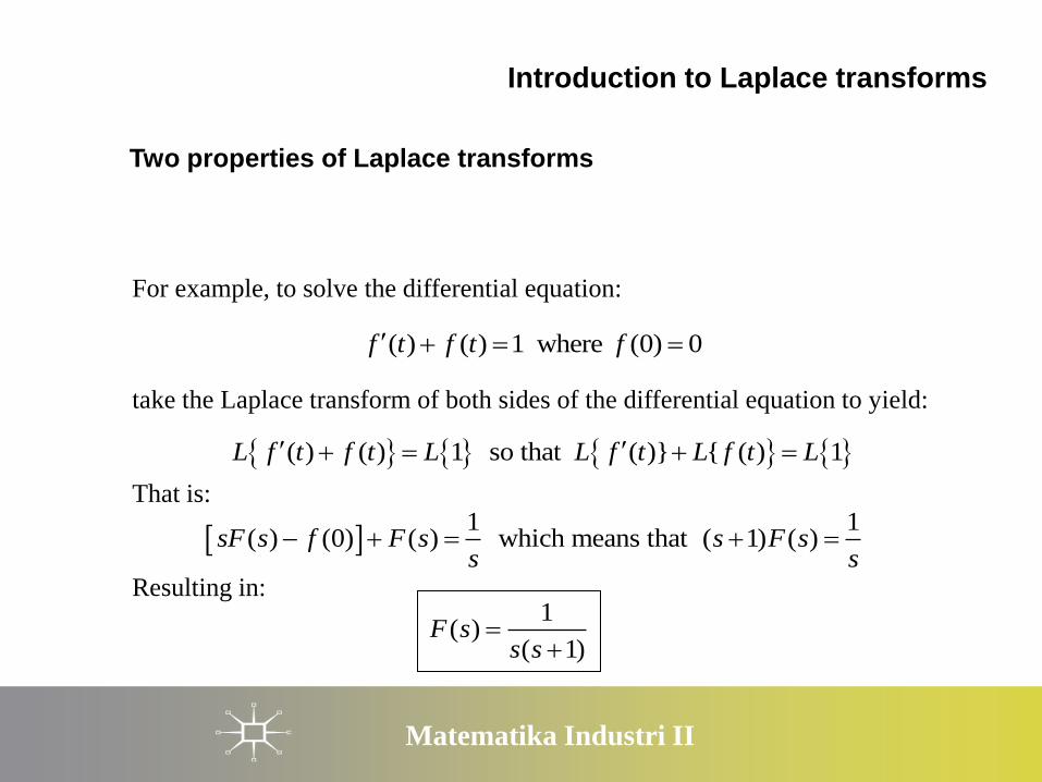
For example, to solve the differential equation:

take the Laplace transform of both sides of the differential equation to yield:

That is:

Resulting in:

( ) ( ) 1 where (0) 0f t f t f

( ) ( ) 1 so that ( )} { ( ) 1L f t f t L L f t L f t L

1 1

( ) (0) ( ) which means that ( 1) ( )sF s f F s s F ss s

1( )

( 1)F s

s s




Given that:

The right-hand side can be separated into its partial fractions to give:

From the table of transforms it is then seen that:

1( )

( 1)F s

s s

1 1( )

1F s

s s

1

1 1

1 1( )

1

1 1

1

1 t

f t Ls s

L Ls s

e




Thus, using the Laplace transform and its properties it is found that the

solution to the differential equation:

is:

( ) 1 tf t e

( ) ( ) 1 where (0) 0f t f t f


Bahasan










Generating new transforms

Deriving the Laplace transform of f (t ) often requires integration by parts.

However, this process can sometimes be avoided if the transform of the

derivative is known:

For example, if f (t ) = t then f ′ (t ) = 1 and f (0) = 0 so that, since:

That is:

( ) { ( )} (0) then {1} { } 0L f t sL f t f L sL t

2

1 1{ } therefore { }sL t L t

s s


Bahasan










Laplace transforms of higher derivatives

It has already been established that if:

then:

Now let

so that:

Therefore:

( ) { ( )} and ( ) { ( )}F s L f t G s L g t

( ) ( ) so (0) (0) and ( ) ( ) (0)g t f t g f G s sF s f

{ ( )} { ( )} ( ) (0)

( ) (0) (0)

L g t L f t sG s g

s sF s f f

2{ ( )} ( ) (0) (0)L f t s F s sf f

𝐿 𝑓′ 𝑡 = 𝑠𝐹 𝑠 − 𝑓 0 𝑑𝑎𝑛 𝐿 𝑔′ 𝑡 = 𝑠𝐺 𝑠 − 𝑔(0)




For example, if:

then:

and

Similarly:

And so the pattern continues.

( ) { ( )}F s L f t

2{ ( )} ( ) (0) (0)L f t s F s sf f

3 2{ ( )} ( ) (0) (0) (0)L f t s F s s f sf f

𝐿 𝑓′ 𝑡 = 𝑠𝐹 𝑠 − 𝑓 0




Therefore if:

Then substituting in:

yields

So:

2( ) sin so that ( ) cos and ( ) sinf t kt f t k kt f t k kt

2{ ( )} ( ) (0) (0)L f t s F s sf f

2 2 2{ sin } {sin } {sin } .0L k kt k L kt s L kt s k

2 2{sin }

kL kt

s k



Table of Laplace transforms

In this way the table of Laplace transforms grows:

1

2 2

2 2

2 2

2 2

( ) { ( )} ( ) { ( )}

sin 0

cos 0

f t L F s F s L f t

kkt s k

s k

skt s k

s k

1

2

( ) { ( )} ( ) { ( )}

0

1

1

( )

kt

kt

f t L F s F s L f t

kk s

s

e s ks k

te s ks k




Learning outcomes

Derive the Laplace transform of an expression by using the integral definition

Obtain inverse Laplace transforms with the help of a table of Laplace transforms

Derive the Laplace transform of the derivative of an expression

Solve linear, first-order, constant coefficient, inhomogeneous differential equations

using the Laplace transform

Derive further Laplace transforms from known transforms

Use the Laplace transform to obtain the solution to linear, constant-coefficient,

inhomogeneous differential equations of second and higher order.



Reference

• Stroud, KA & DJ Booth. 2003. Matematika

Teknik. Erlangga. Jakarta

Documents

DASAR TRANSFORMASI LAPLACE - Universitas Brawijaya · (2) The transform of an expression that is multiplied by a constant is the constant multiplied by the transform. That is: ^ `