Darmstadt Discussion Papers in Economics

Rational Actors in Balancing Markets: a Game-Theoretic Model and Results

Thomas Rupp

Nr. 171

Arbeitspapiere des Instituts für Volkswirtschaftslehre

Technische Universität Darmstadt

A R E

pplied

conomics

esearch in

Rational Actors in Balancing Markets: a

Game-Theoretic Model and Results

Thomas Rupp∗

Keywords:

game theory, nash equilibrium, regulated energy market, balancing power

JEL classification: C73, D58, Q41, D40

May 31, 2006

Abstract

Guided by game theory we develop a model to explain behavioral equi-libria under uncertainty and interaction with the spot market on balancingmarkets. We offer some insights for the general model and derive explicitsolutions for a specific model in which the error distributions and pric-ing function are given. The most interesting conclusions are the uniqueexistence of an equilibrium and that no participant acts contrary to theaggregate market (either all market participants buy or sell power) andall strategies are, normalized properly, equal (which is rather counter-intuitive). Furthermore the aggregate behavior is a stochastic processvarying around its own variance.

∗Department of Applied Economics and Microeconometrics, Institute of EconomicsDarmstadt University of TechnologyTel.: +49 (0)6151 16-5512, Fax: +49 (0)6151 16-5652email: rupp@vwl.tu-darmstadt.de

1

1

1 Introduction

Industrialized countries need steady and reliable electricity supply. Modeling the

electricity market is typically analyzed with either Supply-Function-Equilibria

(for examples refer to Klemperer and Meyer (1989), Green and Newbery (1992),

Green (1996), Weber and Overbye (1999) or Berry et al. (1999a)), with Cournot-

models (e.g. Cardell et al. (1997), Hogan (1997), Hobbs et al. (2000), Boisseleau

et al. (2004)) or Stackelberg-models (e.g. Wolf and Smeers (1997) or Chen et al.

(2004)). The former is a better fit to the technical realization of many electricity

markets where bids are given as supply or cost functions.

The electricity market is a forward market with a single not-storeable good (see

Allaz (1992), Allaz and Vila (1993) or Green and Newbery (1992)). The game-

theoretic literature usually deals with a two-stage approach with power generators

choosing their investment (or, in fact, their capacity) in the first stage and the

price in the second (von der Fehr and Harbord (1997), Coq (2002) and Sanin

(2005)). Introductions to energy market models can be found in Meibom et al.

(2003), Boisseleau et al. (2004), Yao et al. (2004) and Sanin (2005).

We use a simultaneous one-stage approach which is fundamentally different from

the usual models and is solely based on the uncertainty of the demand for power

and the price on the spot market. This Cournot-Model consists of two phases:

1. In the first phase all participants (henceforth called players) buy and sell

energy on the spot market (or wholesale market) at a given price. To

simplify analysis we assume that the price is public knowledge.

2. The players cannot act in the second phase. The actual aggregate balance

of power is determined as well as the power balance for every player. A

transmission system operator (TSO) ensures that demand and supply are

in balance. Depending on the aggregate power balance the TSO prices

power with a high price if the aggregate market is short on power or a low

price otherwise.

Every player who is short on power is charged with the fixed price (by the

TSO) and all players who bought too much power are compensated. This

is the balancing power market (or regulating power market).

Three questions immediately arise.

• How much power should each player buy on the spot market?

2 1 INTRODUCTION

• How can the TSO regulate the players (which price should be set to suppress

strategic power trading)?

• Is there an (unique) equilibrium solution at all?

Regarding the last question Sanin (2005) find such an equilibrium but she used

a quite different set of assumptions. In our model this is also true for a realistic

case but must not hold in more general cases since the functions of the expected

utilities are not convex.

It is not trivial at all that an equilibrium should exist anyway since every player

has an incentive to behave contrary to the aggregate market. The price of power

will be low if the aggregate market buys too much, and it is therefore better to

buy less than the expected demand since the charged price will be low. Similarly

there is an incentive to buy too much power if the aggregate market will be low on

power, since the compensating price will be high. This suggests that there should

be either no nash equilibrium besides buying the expected amount of power or

the decision to buy more/less than the expected demand should depend on the

variance of the actual demand1. It turns out that neither must be the case.

In the case that the expected price on the balancing market equals the spot

price, intuition suggests that the power bought by all players should be equal

to the expected demand. It turns out that this depends (at least) on the price

function of the TSO. Moreover, under reasonable assumptions, the real price on

the balancing power market does not matter - only the difference between the

minimum and maximum price is relevant.

1.1 Distinction from related literature

We explicitly neglect several characteristics which are commonly part of the

widely used models. We do not consider the (double)-auction mechanisms (

e.g. Wolfram (1998), Supatgiat et al. (2001), Wolak (2000), Baldick et al. (2004)

or Boisseleau et al. (2004)) to calculate prices on either the spot- or the balanc-

ing market. We are also not concerned with the technical distribution of power

(e.g. Berry et al. (1999b), Kleindorfer et al. (2000) or Willems (2006)) or the

behavior of the power generators and therefore neglect any constraints given by

1The reasoning could be that players with high variance have an incentive to buy largeramounts of strategic power to insure them against unexpected high prices; this could be ex-ploited, ceteris paribus, by players with low variance.

3

the generators (as in Berry et al. (1999b), Supatgiat et al. (2001), Yao et al.

(2004), Sweeting (2004) or Holmberg (2004)). These are no serious limitations

since the price on the balancing market can vary in every round, as long as every-

thing is public knowledge. Additionally we assume that buying strategic power

(which means buying intentionally more or less than the expected demand) is not

punished. In Germany this is forbidden by law (see for example RWE (2006))

but there has been no actual prosecution in Germany2 although such behavior is

obvious (Rupp, 2003).

The model we present provides a new, straight forward and easy way to verify

whether an energy market has reached its equilibrium state and to understand

why the aggregate power on the balancing market does not necessarily vary

around zero. Additionally we offer a convenient way to see how the prices on

the balancing market influence the market behavior. We start with a general set-

ting with risk-neutral players and than proceed to normal distributed forecasting

errors and a specific pricing function3 for the balancing market.

The paper is organized in the following way: section 2 discusses the model, section

3 includes some results of the most general case when (almost) no assumptions

are made about the model parameters, while section 4 and 5 derive the important

results for models with normal errors and two specific pricing functions. Section

6 concludes the paper with a short discussion. The bulk of the appendix contains

the long proofs of some propositions in section 4 and 5.

2 The Model

Basically the model consists of the stochastic error of each player (difference of

predicted and actual power demand of all respective end customers), the strate-

gically bought power on the spot market by each player and the pricing function

of the TSO.

• X := (X1, . . . , Xn) is a Rn−valued random variable, whereas Xi is the power

demand (of all end customers) of player i

2Private correspondence with a manager of a large energy company.3The binary function fits the German balancing market reasonably well. For more informa-

tion about the German energy market refer to Swider and Weber (2000), Rupp (2003), Meibomet al. (2003) or RWE (2006) for a specific example.

4 2 THE MODEL

– σ2i := Var(Xi), 0 ≤ σ2

i < ∞

– µ := (µ1, . . . , µn) ∈ Rn and µi := E[Xi]

– X1, X2, . . . , Xn are mutually independent and have a density

• v := (v1, . . . , vn) ∈ Rn, whereas vi is the amount of power strategically

bought by player i

• ps is the price paid on the spot market

• M = M(X, µ, v) :=n∑

i=1

(Xi − (µi + vi)) is the aggregate unsatisfied demand

for power

• pb = f(M) is the price on the balancing market fixed by the TSO, deter-

mined with the pricing function f(M) which fulfills the following conditions:

– ∃M ≥ 0 : M ≥ M ⇔ f(M) ≥ ps

– f is monotonically increasing, non-negative and bounded

– f is continuous in sections

• Gi(vi) = Gi(X, µ, v) := (µi + vi −Xi)f(M) − vipb is the monetary gain of

player i

All players are fully informed (they know all parameters and functions), all act

independently and simultaneously in every round and all players maximize their

expected profit. Thus we have to deal with a typical open ended game theoretic

problem under full information.

Given all information we have to find all vectors v∗ which satisfy

E[Gi(v∗)] ≥ E[Gi(vi|vj = v∗j ∀j 6= i)] i = 1 . . . n. (1)

Without loss of generality we can set µ = 0 since we can otherwise define X′ :=

X − µ and v′ := v − µ. Then (v − X) is distributed as (v′ − X′) - the expected

demand would simply be adjusted by the strategic amount of power.

Since the global condition given by equation (1) is hard to analyze we restrict

ourselves to the commonly used local equilibrium conditions: the first derivative

of E[Gi(v)] must be zero for all i:

∂∂vi

E[Gi(v)] = 0

⇔ E[(vi −Xi)

∂∂vi

f(M)]

+ E[f(M)]− ps = 0

⇔ E[(vi −Xi)

∂∂M

f(M)]

= E[f(M)]− ps.

2.1 Intuition 5

We can rewrite these equations as

E [(vi −Xi)f′(M)] = E[f(M)]− ps, (2)

E [(vi −Xi)f′(M)] = E [(vj −Xj)f

′(M)] ∀i, j. (3)

These local conditions imply an equilibrium only for marginal deviations. In the

case of non-convex Gi’s there might be multiple local equilibria which might be

global maxima only for different subsets of players. Henceforth we always refer

to local equilibria, unless stated otherwise.

2.1 Intuition

There are several basic concepts which seem to be easily applicable to the model

but eventually are not - at least not in the more specific models which are acces-

sible to further analysis.

2.1.1 Existence of equilibria

As already mentioned in the introduction, intuition suggests that there should be

either no equilibrium at all (except v = 0) or the signs of the vi should depend

on σ2i .

A player should, since he knows the expected amount of power of the aggregate

market when all other players strategies are fixed, do the opposite as the aggregate

market does: buy more power if the aggregate market is expected to be low on

power and buy less otherwise. Only in the case that the aggregate market balance

is expected to be zero and the expected price equals the price on the spot market,

v = 0, should be a nash equilibrium. While the latter property holds in the

specific models, the former does not.

It would also be intuitive if the sign of each individual would at least depend on

the variances of the Xi. Players with large variances should be more concerned

to drive the market in one direction to avoid, for example, being charged with

high prices on the balancing power market (when the spot price is comparably

low). This should be exploitable by players with low variances.

It turns out in the specific models that the strategies of all players share the same

sign and, when normalized, are essentially all equal.

6 3 THE GENERAL MODEL

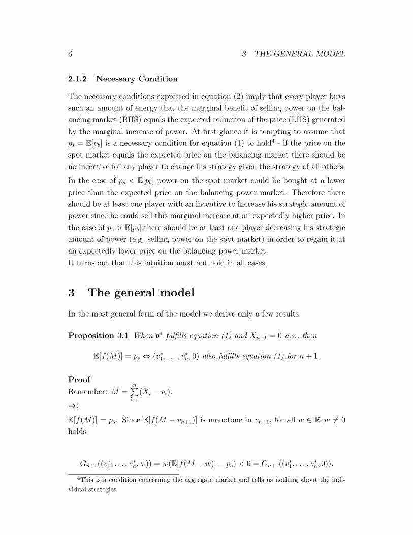
2.1.2 Necessary Condition

The necessary conditions expressed in equation (2) imply that every player buys

such an amount of energy that the marginal benefit of selling power on the bal-

ancing market (RHS) equals the expected reduction of the price (LHS) generated

by the marginal increase of power. At first glance it is tempting to assume that

ps = E[pb] is a necessary condition for equation (1) to hold4 - if the price on the

spot market equals the expected price on the balancing market there should be

no incentive for any player to change his strategy given the strategy of all others.

In the case of ps < E[pb] power on the spot market could be bought at a lower

price than the expected price on the balancing power market. Therefore there

should be at least one player with an incentive to increase his strategic amount of

power since he could sell this marginal increase at an expectedly higher price. In

the case of ps > E[pb] there should be at least one player decreasing his strategic

amount of power (e.g. selling power on the spot market) in order to regain it at

an expectedly lower price on the balancing power market.

It turns out that this intuition must not hold in all cases.

3 The general model

In the most general form of the model we derive only a few results.

Proposition 3.1 When v∗ fulfills equation (1) and Xn+1 = 0 a.s., then

E[f(M)] = ps ⇔ (v∗1, . . . , v∗n, 0) also fulfills equation (1) for n + 1.

Proof

Remember: M =n∑

i=1

(Xi − vi).

⇒:

E[f(M)] = ps. Since E[f(M − vn+1)] is monotone in vn+1, for all w ∈ R, w 6= 0

holds

Gn+1((v∗1, . . . , v

∗n, w)) = w(E[f(M − w)]− ps) < 0 = Gn+1((v

∗1, . . . , v

∗n, 0)).

4This is a condition concerning the aggregate market and tells us nothing about the indi-vidual strategies.

7

⇐:

Assume E[f(M)] 6= ps. Since E[f(M − vn+1)] is affine linear in vn+1, there exists

a w ∈ R, w 6= 0 which fulfills

Gn+1((v∗1, . . . , v

∗n, w)) = w(E[f(M − w)]− ps) > 0 = Gn+1((v

∗1, . . . , v

∗n, 0)).

Therefore (v∗1, . . . , v∗n, w) does not fulfill equation (1) for any w 6= 0, whereas

w = 0 removes player n + 1 from the market system.

�

Definition 3.2 (Closed market) We call a market closed when there is no

incentive for other players (who are not forced to participate in the market, e.g.

players with zero variance) to join the market5.

It sounds reasonable that the market should always be closed since otherwise (up

to to an infinite number of) players could join the system. The market is closed

anyway when either v∗ = 0 or Gi(v∗) ≤ 0,∀i > n.

Corollary 3.3 When the expected price on the balancing power market equals

the spot price the former market is closed: E[f(M)] = ps ⇒ the balancing power

market is closed.

4 The specific model

To derive specific results analytically we introduce some further assumptions.

We begin with a more general class of pricing function f to subsequently derive

afterwards specific results with a binary f . We assume furthermore that all Xi

are normally distributed.

5Unlike in other markets the TSO must always, at least in theory, satisfy every demand onthe balancing market.

8 4 THE SPECIFIC MODEL

4.1 f as the error-function

Let f be given by

f(M) = f(M, a, ph, pl) :=(ph − pl)

2(erf(aM) + 1) + pl. (4)

The error-function erf(x) is by definition 2√π

x∫0

e−t2dt. The parameter a controls

the slope around M = 0. More details are given in the appendix A.1.

To simplify notation we define

V :=n∑

k=1

vk and S2 :=n∑

k=1

σ2k as well as Vi := V − vi and S2

i := S2 − σ2i .

Thus we can write E[M ] = −V and Var(M) = S2, hence

M ∼ N (−V, S2).

4.2 Equilibria

Necessary conditions for the nash equilibrium (equation (1)) to hold for a v∗

are that the first derivatives of the Gi are zero and the second derivatives are

negative. It is then sufficient to show that the local maximum attained is the

global maximum for each player and the relationship between all v∗i is unique.

In the specific model we derive the necessary conditions which are sufficient for

local equilibria.

Theorem 4.1 Let all Xi be normally distributed and f as given in equation (4).

The (not necessarily unique) local nash equilibrium, given by equations (2) and

(3), is determined by the following conditions

v∗j =2na2σ2

j + 1

2na2σ21 + 1

v∗1 , j = 2, . . . , n,

E[f(M∗)]− ps = E [(v∗1 −X1)f′(M∗)]

There are either one or two local equilibria.

The proof is given in appendix A.1. The theorem establishes the conditions for

local equilibriums. In such a situation no player will deviate from his current

strategy by any small amount. However, we emphasize that the possibility that

a player may achieve a higher benefit, if he deviates by a large amount, is not

ruled out in general.

4.2 Equilibria 9

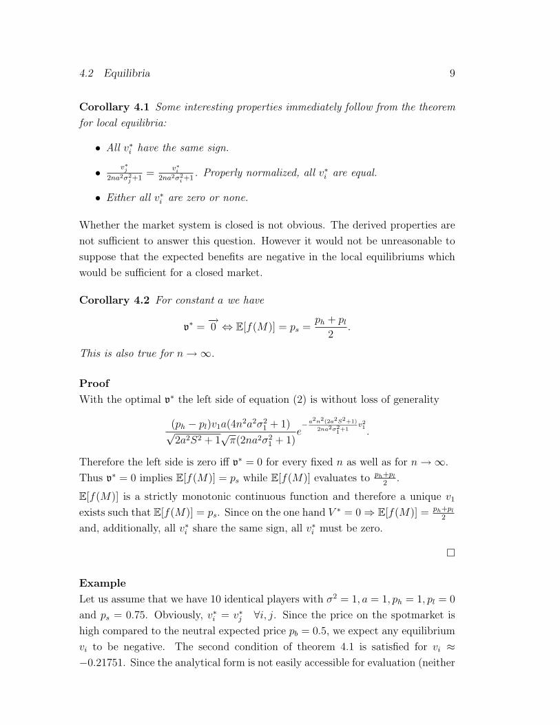
Corollary 4.1 Some interesting properties immediately follow from the theorem

for local equilibria:

• All v∗i have the same sign.

• v∗j2na2σ2

j +1=

v∗i2na2σ2

i +1. Properly normalized, all v∗i are equal.

• Either all v∗i are zero or none.

Whether the market system is closed is not obvious. The derived properties are

not sufficient to answer this question. However it would not be unreasonable to

suppose that the expected benefits are negative in the local equilibriums which

would be sufficient for a closed market.

Corollary 4.2 For constant a we have

v∗ =−→0 ⇔ E[f(M)] = ps =

ph + pl

2.

This is also true for n →∞.

Proof

With the optimal v∗ the left side of equation (2) is without loss of generality

(ph − pl)v1a(4n2a2σ21 + 1)√

2a2S2 + 1√

π(2na2σ21 + 1)

e−a2n2(2a2S2+1)

2na2σ21+1

v21.

Therefore the left side is zero iff v∗ = 0 for every fixed n as well as for n →∞.

Thus v∗ = 0 implies E[f(M)] = ps while E[f(M)] evaluates to ph+pl

2.

E[f(M)] is a strictly monotonic continuous function and therefore a unique v1

exists such that E[f(M)] = ps. Since on the one hand V ∗ = 0 ⇒ E[f(M)] = ph+pl

2

and, additionally, all v∗i share the same sign, all v∗i must be zero.

�

Example

Let us assume that we have 10 identical players with σ2 = 1, a = 1, ph = 1, pl = 0

and ps = 0.75. Obviously, v∗i = v∗j ∀i, j. Since the price on the spotmarket is

high compared to the neutral expected price pb = 0.5, we expect any equilibrium

vi to be negative. The second condition of theorem 4.1 is satisfied for vi ≈−0.21751. Since the analytical form is not easily accessible for evaluation (neither

10 5 THE BINARY MODEL

exact nor numerical), we performed some simulations which indicate that this v∗

is the global maximum for all players and the expected benefits are negative.

Thus this seems to be a true nash equilibrium as defined by equation (1) and is

minimizing the losses of all players. Since there is no expected benefit for any

additional player (the new equilibrium for n = 11, σ11 = 0 also yields negative

benefits) the market is closed.�

5 The binary model

A specific sub-model of the model presented in section 4, which can be analyzed

in more detail, is attained by taking the limits a → ∞, which transforms the

pricing function into an indicator function

f(M) =

ph if M ≥ 0

pl otherwise.(5)

All previous results can now be easily reevaluated - analyzing G in the binary

model beforehand had been impractical. A binary pricing function is not a bad

approximation, as can be seen in RWE (2006) or Rupp (2003), in the the case of

the RWE-balancing market in Germany.

Theorem 5.1 Let all Xi be normally distributed, f be given as in equation (5)

and Φ−1 be the inverse of the normal distribution function. The unique global

nash equilibrium, given by equation (1), is determined by

v∗i =σ2

i

SΦ−1

(ph − ps

ph − pl

). (6)

The proof is given in appendix A.3.

Corollary 5.1 (The market process) Let λ := Φ−1([ph − pz]/[ph − pn]) and

X =∑n

i=1 Xi then summation over all players leads to the following process

characterization:

M = −λ√

Var(X) + X.

11

Thus the demand of power on the balancing market is a stochastic process driven

by two different components: the variance of the actual demand of all players, the

distance from the spotmarket price to the upper price cap and the price bandwith

on the balancing market.

When the prices do not vary (i.e. λ is a constant) the process M solely varies

around its own variance (with the mean −λ√

Var(X) and the noise term X).

Thus, given a negative λ, the process is driven upwards (downwards) if the vari-

ance of X increases (decreases). Naturally the variance of M is the same as the

variance of X. This is a curious result because such processes are not commonly

found in practice.

In contrast to the previous setting, the following corollary is proven to hold:

Corollary 5.2 E[f(M)] = ps and therefore the market system is closed.

The proof is part of the proof of theorem 5.1. The corollary from the previous

section can be transferred one-to-one.

Corollary 5.3

• All v∗i have the same sign.

• v∗jσ2

j=

v∗iσ2

i. Properly normalized all v∗i are equal.

• Either all v∗i are zero or none.

The binary pricing function also implies

Corollary 5.4 Only the span between the high and low price cap is relevant - the

absolute prices do not matter. Without loss of generality the TSO can set pl = 0

and influence the market by varying the high price ph.

6 Conclusion

Motivated by the balancing power market system we have developed a one-stage

game-theoretic model to describe optimal behavior of rational players on balanc-

ing markets. In such a system players buy power on a spot market and then the

unsatisfied power demand is traded automatically on the balancing power market

at a given price (depending on the aggregate demand of power of all customers).

12 6 CONCLUSION

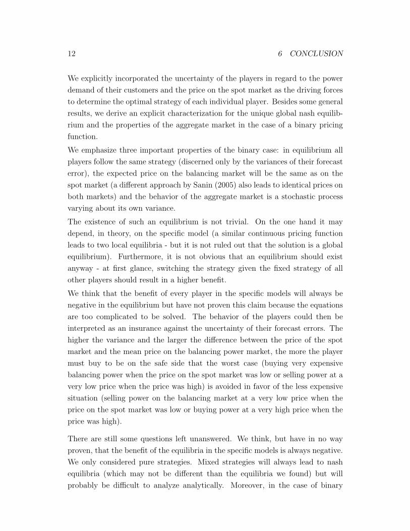
We explicitly incorporated the uncertainty of the players in regard to the power

demand of their customers and the price on the spot market as the driving forces

to determine the optimal strategy of each individual player. Besides some general

results, we derive an explicit characterization for the unique global nash equilib-

rium and the properties of the aggregate market in the case of a binary pricing

function.

We emphasize three important properties of the binary case: in equilibrium all

players follow the same strategy (discerned only by the variances of their forecast

error), the expected price on the balancing market will be the same as on the

spot market (a different approach by Sanin (2005) also leads to identical prices on

both markets) and the behavior of the aggregate market is a stochastic process

varying about its own variance.

The existence of such an equilibrium is not trivial. On the one hand it may

depend, in theory, on the specific model (a similar continuous pricing function

leads to two local equilibria - but it is not ruled out that the solution is a global

equilibrium). Furthermore, it is not obvious that an equilibrium should exist

anyway - at first glance, switching the strategy given the fixed strategy of all

other players should result in a higher benefit.

We think that the benefit of every player in the specific models will always be

negative in the equilibrium but have not proven this claim because the equations

are too complicated to be solved. The behavior of the players could then be

interpreted as an insurance against the uncertainty of their forecast errors. The

higher the variance and the larger the difference between the price of the spot

market and the mean price on the balancing power market, the more the player

must buy to be on the safe side that the worst case (buying very expensive

balancing power when the price on the spot market was low or selling power at a

very low price when the price was high) is avoided in favor of the less expensive

situation (selling power on the balancing market at a very low price when the

price on the spot market was low or buying power at a very high price when the

price was high).

There are still some questions left unanswered. We think, but have in no way

proven, that the benefit of the equilibria in the specific models is always negative.

We only considered pure strategies. Mixed strategies will always lead to nash

equilibria (which may not be different than the equilibria we found) but will

probably be difficult to analyze analytically. Moreover, in the case of binary

13

pricing functions the results may hold regardless of the kind of distribution of the

error terms (as long as they have continuous densities). Although we have reasons

to doubt, other pricing functions may lead to different results. It would also

be interesting to incorporate stepwise pricing functions or a covariance structure

(removing the independence assumption) or to answer the question whether there

is any model specification which allows differently signed6 optimal strategies.

In an upcoming paper we apply this model to the German balancing power market

of the RWE zone and show that the data can be applied to the binary model

and the behavior of the aggregate market can be replicated as soon as the prices

of the spotmarket (taken from the EEX, the European Power Exchange stock

market, EEX (2006)) become similar to the mean prices of the balancing power

market (which has in fact been the case for the last two years 2004 and 2005).

A Appendix

A.1 The price function f(M)

The following graphs show f with ph = 9, pl = 1 and a = 0.5, 1 and 2:

This function fulfills all conditions given in section 2 and is infinitely often dif-

ferentiable

The first and second derivatives are

∂

∂Mf(M) =

a(ph − pl)√π

e−(aM)2 and∂2

∂M2f(M) =

−2a3(ph − pl)M√π

e−(aM)2 .

This function does not fit very well for realistic prices where M is near zero.

Prices near the mean value of the high and low price caps are only rarely seen in

Germany. Nevertheless, this function is still important since its main purpose is

to analytically tackle the binary case.

6Equilibria in which some market participants buy and some sell strategic power.

14 A APPENDIX

A.2 Proof of Theorem 4.1

Proof Equation (2) is the second condition in the theorem. The first condition

refers to equation (3) and can be written explicitly and simplified:

∀i, j :1

σi

√2π

∞∫−∞

(vi − x)e− x2

2σ2i

∞∫−∞

a(ph − pl)√π

e−(a(x+y−V ))2 e− y2

2S2i

Si

√2π

dydx

=1

σj

√2π

∞∫−∞

(vj − x)e− x2

2σ2j

∞∫−∞

a(ph − pl)√π

e−(a(x+y−V ))2 e− y2

2S2j

Sj

√2π

dydx

⇔ (ph − pl)(vi + 2a2viS2i + 2a2viσ

2i − 2a2σ2

i V )ae− V 2a2

1+2a2S2i+2a2σ2

i

(1 + 2a2S2i + 2a2σ2

i )32√

π

=(ph − pl)(vj + 2a2vjS

2j + 2a2vjσ

2j − 2a2σ2

j V )ae− V 2a2

1+2a2S2j+2a2σ2

j

(1 + 2a2S2j + 2a2σ2

j )32√

π.

Since by definition 2a2S2k + 2a2σ2

k = 2a2S2 for all k, we can rewrite these rela-

tionships to

∀i, j : vi + 2a2viS2 − 2a2σ2

i (Vj + vj) = vj + 2a2vjS2 − 2a2σ2

j (Vj + vj)

⇔ ∀i, j :vi + 2a2viS

2 − 2a2Vj(σ2i − σ2

j )

1 + 2a2S2 + 2a2(σ2i − σ2

j )= vj. (7)

In the next steps we show that the v∗i given in the theorem is a solution for

these relationships. Since the equations (3) form a linear equation-system with

n unknown parameters and n− 1 independent equations the derived relationship

is unique7 (in other words: every solution has one degree of freedom). We then

proceed to show that the second derivative has two roots. Since E[Gi] tends

to −∞ as vi tends to ±∞ and is continuous there exist two local maxima and

one local minima8. Therefore, the last free v1 is determined by the largest local

maxima.

We have to show that

vi + 2a2viS2 − 2a2Vj(σ

2i − σ2

j )

1 + 2a2S2 + 2a2(σ2i − σ2

j )=

2na2σ2j + 1

2na2σ2i + 1

vi

7Players with identical variances just reduce the number of equations.8As is shown later, these three local extremals collapse to one when the parameter a or n

tends to infinity.

A.2 Proof of Theorem 4.1 15

holds:

vi + 2a2viS2 − 2a2Vj(σ

2i − σ2

j )

1 + 2a2S2 + 2a2(σ2i − σ2

j )

=vi + 2a2viS

2

1 + 2a2S2 + 2a2(σ2i − σ2

j )−

2a2vi

2na2σ2i +1

n∑k=1k 6=j

2na2σ2k + 1

(σ2i − σ2

j )

1 + 2a2S2 + 2a2(σ2i − σ2

j )

=(vi + 2a2viS

2)(2na2σ2i + 1)− 2a2vi(σ

2i − σ2

j )(2na2S2j + n− 1)

(1 + 2a2S2 + 2a2[σ2i − σ2

j ])(2na2σ2i + 1)

=vi

2na2σ2i + 1

((1 + 2a2S2)(2na2σ2

i + 1)− 2a2(σ2i − σ2

j )(2na2S2j + n− 1)

1 + 2a2S2 + 2a2(σ2i − σ2

j )

)=

vi

2na2σ2i + 1

((1 + 2a2S2)(1 + 2na2σ2

j ) + (4na4σ2j + 2a2)(σ2

i − σ2j )

1 + 2a2S2 + 2a2(σ2i − σ2

j )

)=

vi

2na2σ2i + 1

((1 + 2a2S2)(1 + 2na2σ2

j ) + (1 + 2na2σ2j )2a

2(σ2i − σ2

j )

1 + 2a2S2 + 2a2(σ2i − σ2

j )

)=

2na2σ2j + 1

2na2σ2i + 1

vi

The second derivative is

∂2

∂v2i

E[Gi(v)]

=∂

∂vi

(E

[(vi −Xi)

∂

∂vi

f(M)

]+ E[f(M)]

)=

∂

∂vi

(−E

[(vi −Xi)

∂

∂Mf(M)

])− ∂

∂ME[f(M)]

= E[(vi −Xi)

∂2

M2f(M)

]− 2E

[∂

∂Mf(M)

]=

∞∫−∞

(vi − x)√2πσ2

i

e−x2

2σ2i

∞∫−∞

1√2πS2

i

e−y2

2S2i−2a3(ph − pl)(y + x− V )√

πe−a2(y+x−V )2dydx

−2

∞∫−∞

1√2πS2

e−x2

2S2a(ph − pl)√

πe−a2(x−V )2dx

= −2(ph − pl)a−e

− a2V 2

1+2a2S2

(1 + 2a2S2)5/2√

π

[a4(4S4 − 2S2V vi − 2S2σ2

i + 2V 2σ2i )

+a2(4S2 − V vi − σ2i ) + 1

]

16 A APPENDIX

Without loss of generality we set i = 1 and use vj =2na2σ2

j +1

2na2σ21+1

v1 and V =2na2S2+n2na2σ2

1+1v1. The second derivative then has the following two roots:

± 2na2σ21 + 1

a√

2na2S2 + n

√2a2S2 − a2σ2

1 + 1.

Therefore for every a and n there are two v∗ which satisfy the local equilibrium

conditions - the final vector is then given by the larger E[G1(v∗)].

�

A.3 Proof of theorem 5.1

Proof

1. Theorem 4.1 and equation (3) lead to

v∗j = lima→∞

2na2σ2j + 1

2na2σ2i + 1

v∗i =σ2

j

σ2i

v∗i and therefore V ∗i =

n∑j=1,j 6=i

v∗j =v∗iσ2

i

S2i .

2. Now condition (2) can be expressed as

lima→∞

E[(v∗i −X)f ′(M)] = E[f(M)]− ps

⇔ lima→∞

(ph − pl)(v∗i + 2a2v∗i S

2i − 2a2σ2

i V∗i )ae

− V ∗2a2

1+2a2S2

(1 + 2a2S2)32√

π= E[f(M)]− ps

⇒ (ph − pl)(v∗i S

2i − σ2

i V∗i )e−

V ∗2

2S2

√2πS3

= E[f(M)]− ps

⇔(ph − pl)(v

∗i S

2i − σ2

iv∗iσ2

iS2

i )e−V ∗2

2S2

√2πS3

= E[f(M)]− ps

⇔ 0 = E[f(M)]− ps

Therefore we have E[f(M)] = ps in any equilibrium.

3. V ∗ = v∗iS2

σ2i. The vector v∗ is unique, since the only free variable v∗i has a a

REFERENCES 17

single solution in equation (2):

E[f(M)] = ps

⇔ P (M ≥ 0)ph + [1− P (M ≥ 0)]pl = ps

⇔ P (M ≥ 0)(ph − pl) = (ps − pl)

⇔ P (X ≥ V ∗) =ps − pl

ph − pl

⇔ P (X < V ∗) =ph − ps

ph − pl

⇔ P

(X < v∗i

S2

σ2i

)=

ph − ps

ph − pl

⇔ v∗iS

σ2i

= Φ−1

(ph − ps

ph − pl

)⇔ v∗i =

σ2i

SΦ−1

(ph − ps

ph − pl

)

Therefore we have a single unique extremal which has to be a global maximum.

Plugging V into the second derivative from the appendix A.2 and taking the

limit9 a →∞ the second derivative now becomes

−(ph − pl)(2S2 − σ2

1)√2πS3

e−S2v2

12σ4

1 < 0.

�

References

Allaz, B. (1992). “Oligopoly, Uncertainty and Strategic Forward Transactions.”

International Journal of Industrial Organization. 10 (2), 297–308.

and J. L. Vila (1993). “Cournot Competition, Forward Markets and

Efficiency.” Journal of Economic Theory. 59 (1), 1–16.

Baldick, R., R. Grant, and E. Kahn (2004). “Theory and Application of Linear

Supply Function Equilibrium in Electricity Markets.” Journal of Regulatory

Economics. 25 (2), 143–167.

9The limit n →∞ also leads to a strictly negative second derivation.

18 REFERENCES

Berry, C. A., B. F. Hobbs, W. A. Meroney, R. P. O’Neill, and W. R. Stewart Jr.

(1999a). “Analyzing Strategic Bidding Behavior in Transmission Networks.”

Utilities Policy. 8 (3), 139–158.

, , , , and (1999b). “Understanding how

market power can arise in network competition: a game theoretic approach.”

Utilities Policy. 8 (3), 139–158.

Boisseleau, F., T. Kristiansen, and W. van der Veen (2004). “A Supply Func-

tion Equilibrium Model with Forward Contracts - An Application to Whole-

sale Electricity Markets.” Conference Paper, 6th IAEE European Conference,

Zurich.

Cardell, J. B., C. C. Hitt, and W. W. Hogan (1997). “Market power and strategic

interaction in electricity networks.” Resource and Energy Economics. 19 (1-2),

109–137.

Chen, Y., B. F. Hobbs, S. Leyfer, and T. S. Munson (2004). “Leader-Follower

Equilibria for Electric Power and NOx Allowances Markets.” Technical Report

ANL/MCS-P1191-0804 August.

Coq, C. L. (2002). “Strategic use of available capacity in the electricity spot mar-

ket.” Working Paper Series in Economics and Finance 496, Stockholm School

of Economics.

EEX (2006). www.eex.com March.

Green, R. J. (1996). “Increasing Competition in the British Electricity Market.”

Journal of Industrial Economics. 44 (2), 205–216.

and D. M. Newbery (1992). “Competition in the British Electricity Spot

Market.” Journal of Political Economy. 100 (5), 929–953.

Hobbs, B. F., C. B. Metzler, and J. S. Pang (2000). “Strategic Gaming Analysis

for Electric Power Systems: An MPEC Approach.” IEEE Transactions on

Power Systems. 15 (2), 638–645.

Hogan, W. W. (1997). “A market power model with strategic interaction in elec-

tricity markets.” The Energy Journal. 18 (4), 107–141.

REFERENCES 19

Holmberg, P. (2004). “Unique Supply Function Equilibrium with Capacity Con-

straints.” Working Paper Series 2004:20, Uppsala University, Department of

Economics November.

Kleindorfer, P. R., D. J. Wu, and C. Fernando (2000). “Strategic Gaming in

Electric Power Markets.” in “Proceedings of the Proceedings of the 33th Annual

Hawaii International Conference on System Sciences,” IEEE Computer Society,

Washington, DC.

Klemperer, P. D. and M. A. Meyer (1989). “Supply Function Equilibria in

Oligopoly Under Uncertainty.” Econometrica. 57 (6), 1243–1277.

Meibom, P., P. E. Morthorst, L. H. Nielsen, C. Weber, K. Sander, D. Swider, and

H. Ravn (2003). “Power System Models - A Description of Power Markets and

Outline of Marketing Modelling in Wilmar.” Project Report Risø-R-1441(EN),

Risø National Laboratory December.

Rupp, T. (2003). “Gleichgewichte auf Uberschussmarkten - Theorie und Anwend-

barkeit auf die Regelenergiezone der RWE.” Master’s thesis, Johann Wolfgang

Goethe-Universitat Frankfurt am Main, Germany.

RWE (2006). www.rwe-transportnetzstrom.com March.

Sanin, M. E. (2005). “An application of Game Theory to Electricity Markets.”

Working Paper, Universite Catholique de Louvain, Louvain-la-newve, Belgium.

Supatgiat, C., R. Q. Zhang, and J. R. Birge (2001). “Equilibrium Values in a

Competitive Power Exchange Market.” Computational Economics. 17 (1), 92–

121.

Sweeting, A. (2004). “Market Power in the England and Wales Wholesale Elec-

tricity Market 1995-2000.” Cambridge Working Papers in Economics 0455,

Faculty of Economics (DAE), University of Cambridge October.

Swider, D. J. and C. Weber (2000). “Regelenergiemarkt in Deutschland - Aus-

gestaltung und Preisanalyse.” in “Proceedings zur 3. Internationalen En-

ergiewirtschaftstagung an der TU Wien,” TU Wien, Osterreich.

von der Fehr, N.-H. and D. Harbord (1997). “Capacity Investment and Compe-

tition in Decentralized Electricity Markets.” Working Paper 27, University of

Oslo, Department of Economics November.

20 REFERENCES

Weber, J. D. and T. J. Overbye (1999). “A two-level optimization problem for

analysis of market bidding strategies.” in “Proceedings of the IEEE Power

Engineering Society Summer Meeting,” Alberta.

Willems, B. (2006). “Virtual Divestitures, Will They Make A Difference?

Cournot Competition, Option Markets And Efficiency.” Working Paper, Euro-

pean University Institute, Italy January.

Wolak, F. A. (2000). “An Empirical Analysis of the Impact of Hedge Contracts

on Bidding Behavior in a Competitive Electricity Market.” International Eco-

nomic Journal. 14 (2), 1–39.

Wolf, D. D. and Y. Smeers (1997). “A stochastic version of a Stackelberg-Nash-

Cournot equilibrium model.” Management Science. 43 (2), 190–197.

Wolfram, C. D. (1998). “Strategic bidding in a multiunit auction: an empirical

analysis of bids to supply electricity in England and Wales.” RAND Journal

of Economics. 29 (4), 703–725.

Yao, J., S. S. Oren, and I. Adler (2004). “Computing Cournot Equilibria in Two

Settlement Electricity Markets with Transmission Constraints.” in “Proceed-

ings of the Proceedings of the 37th Annual Hawaii International Conference on

System Sciences,” IEEE Computer Society, Washington, DC.

ISSN: 1438-2733