Dark solitons near potential and nonlinearity steps

F. Tsitoura,1 Z. A. Anastassi,2 J. L. Marzuola,3 P. G. Kevrekidis,4, 5 and D. J. Frantzeskakis1

1Department of Physics, University of Athens, Panepistimiopolis, Zografos, Athens 15784, Greece2Department of Mathematics, Statistics and Physics, College of Arts and Sciences, Qatar University, 2713 Doha, Qatar

3Department of Mathematics, University of North Carolina, Chapel Hill, NC 27599, USA4Department of Mathematics and Statistics, University of Massachusetts, Amherst, Massachusetts 01003-4515 USA

5Center for Nonlinear Studies and Theoretical Division,

Los Alamos National Laboratory, Los Alamos, NM 87544

We study dark solitons near potential and nonlinearity steps and combinations thereof, forming rectangular

barriers. This setting is relevant to the contexts of atomic Bose-Einstein condensates (where such steps can be

realized by using proper external fields) and nonlinear optics (for beam propagation near interfaces separating

optical media of different refractive indices). We use perturbation theory to develop an equivalent particle theory,

describing the matter-wave or optical soliton dynamics as the motion of a particle in an effective potential. This

Newtonian dynamical problem provides information for the soliton statics and dynamics, including scenarios

of reflection, transmission, or quasi-trapping at such steps. The case of multiple such steps and its connection

to barrier potentials is additionally touched upon. The range of validity of the analytical approximation and

radiation effects are also investigated. Our analytical predictions are found to be in very good agreement with

the corresponding numerical results, where appropriate.

PACS numbers: 05.45.Yv, 03.75.Lm, 42.81.Dp

I. INTRODUCTION

The interaction of solitons with impurities is a fundamen-

tal problem that has been considered in various branches of

physics – predominantly in nonlinear wave theory [1] and

solid state physics [2] – as well as in applied mathematics (see,

e.g., recent work [3] and references therein). Especially, in

the framework of the nonlinear Schrodinger (NLS) equation,

the interaction of bright and dark solitons with δ-like impuri-

ties has been investigated in many works (see, e.g., Refs. [4–

8]). Relevant studies in the context of atomic Bose-Einstein

condensates (BECs) [9–11] have also been performed (see,

e.g., Refs. [12–16]), as well as in settings involving potential

wells [17, 18] and barriers [19, 20] (see also Ref. [21] for ear-

lier work in a similar model). In this context, localized impu-

rities can be created by focused far-detuned laser beams, and

have already been used in experiments involving dark solitons

[22, 23]. Furthermore, experimental results on the scattering

of matter-wave bright solitons on Gaussian barriers in either7Li [24] or 85Rb [25] BECs have been reported as well. More

recently, such soliton-defect interactions were also explored

in the case of multi-component BECs and dark-bright soli-

tons, both in theory [26] and in an experiment [27].

On the other hand, much attention has been paid to BECs

with spatially modulated interatomic interactions, so-called

“collisionally inhomogeneous condensates” [28, 29]; for a re-

view with a particular bend towards periodic such interac-

tions see also Ref. [30]). Relevant studies in this context

have explored a variety of interesting phenomena: these in-

clude, but are not limited to adiabatic compression of matter-

waves [28, 31], Bloch oscillations of solitons [28], emission

of atomic solitons [32, 33], scattering of matter waves through

barriers [34], emergence of instabilities of solitary waves due

to periodic variations in the scattering length [35], formation

of stable condensates exhibiting both attractive and repulsive

interatomic interactions [36], solitons in combined linear and

nonlinear potentials [37, 38, 40–42], generation of solitons

[43] and vortex rings [44], control of Faraday waves [45], vor-

tex dipole dynamics in spinor BECs [46], and others.

Here, we consider a combination of the above settings,

namely we consider a one-dimensional (1D) setting involv-

ing potential and nonlinearity steps, as well as pertinent rect-

angular barriers, and study statics, dynamics and scattering

of dark solitons. In the BEC context, recent experiments

have demonstrated robust dark solitons in the quasi-1D set-

ting [47]. In addition, potential steps in BECs can be realized

by trapping potentials featuring piece-wise constant profiles

(see, e.g., Refs. [48, 49] and discussion in the next Section).

Furthermore, nonlinearity steps can be realized too, upon em-

ploying magnetically [50] or optically [51] induced Feshbach

resonances, that can be used to properly tune the interatomic

interactions strength – see, e.g., more details in Refs. [33, 38]

and discussion in the next Section.

Such a setting involving potential and nonlinearity steps,

finds also applications in the context of nonlinear optics.

There, effectively infinitely long potential and nonlinearity

steps of constant and finite height, describe interfaces sepa-

rating optical media characterized by different linear and non-

linear refractive indices [52]. In such settings, it has been

shown [53–56] that the dynamics of self-focused light chan-

nels – in the form of spatial bright solitons – can be effectively

described by the motion of an equivalent particle in effective

step-like potentials. This “equivalent particle theory” actu-

ally corresponds to the adiabatic approximation of the per-

turbation theory of solitons [1], while reflection-induced ra-

diation effects can be described at a higher-order approxima-

tion [54, 55]. Note that similar studies, but for dark solitons

in settings involving potential steps and rectangular barriers,

have also been performed – see, e.g., Ref. [57] for an effec-

tive particle theory, and Refs. [58–60] for numerical studies

of reflection-induced radiation effects. However, to the best

of our knowledge, the statics and dynamics of dark solitons

2

near combined potential and nonlinearity steps, have not been

systematically considered so far in the literature, although

a special version of such a setting has been touch upon in

Ref. [38]. In a recent study, [39] considered vortex dynam-

ics in 2d Gross-Pitaevskii and observed that true jumps in the

barriers were quite difficult to using techniques available there

and that some more regularity was required to derive a particle

like picture for vortex dynamics. It is thus rather interesting

that dark solitons can still be handled in such a setting, pro-

vided the jumps are not too large as will be quantified later.

It is our purpose, in this work, to address this problem. In

particular, our investigation and a description of our presenta-

tion is as follows.

First, in Sec. II, we provide the description and modeling

of the problem; although this is done in the context of atomic

BECs, our model can straightforwardly be used for similar

considerations in the context of optics, as mentioned above. In

the same Section, we apply perturbation theory for dark soli-

tons to show that, in the adiabatic approximation, soliton dy-

namics is described by the motion of an equivalent particle in

an effective potential. The latter has a tanh-profile, but – in the

presence of the nonlinearity step – can also exhibit a minimum

and a maximum, i.e., an elliptic and a hyperbolic fixed point,

respectively, in the effective dynamical system. We show that

stationary soliton states do exist at the fixed points, but are un-

stable (albeit in different ways, as is explained below) accord-

ing to a Bogoliubov-de Gennes (BdG) analysis [9–11] that we

perform; we also use an analytical approximation to derive

the unstable eigenvalues as functions of the magnitudes of the

potential/nonlinearity steps.

In Sec. III we study the soliton dynamics for various param-

eter values, pertaining to different forms of the effective po-

tential, including the case of rectangular barriers formed by a

combination of adjacent potential and nonlinearity steps. Our

numerical results – in both statics and dynamics – are found to

be in very good agreement with the analytical predictions. We

also investigate the possibility of soliton trapping in the vicin-

ity of the hyperbolic fixed point of the effective potential; note

that such states could be characterized as “surface dark soli-

tons”, as they are formed at linear/nonlinear interfaces sepa-

rating different optical or atomic media. We show that quasi-

trapping of solitons is possible, in the case where nonlinearity

steps are present; the pertinent (finite) trapping time is found

to be of the order of several hundreds of milliseconds, which

suggests that such soliton quasi-trapping could be observable

in real BEC experiments.

In Sec. IV we extend our considerations beyond the per-

turbative regime and study, in particular, soliton scattering at

larger potential and nonlinearity steps. Our investigation re-

veals both the range of validity of our analytical approxima-

tion and the role of the emission of radiation – in the form

of sound waves – during the scattering process. We find that,

generally, when the soliton moves from a region of larger to-

wards a region of smaller background density, and is scattered

at the discontinuity, then the soliton energy and number of

atoms decrease. The process is such that the difference be-

tween initial and final values of the energy and number of

atoms is equal to the radiation’s respective quantities. Our

pertinent numerical results also reveal the range of validity of

our analytical approach: the latter remains accurate as long

as the percentage strengths of potential/nonlinearity steps are

of the order of 10% of the respective background values, and

fails for larger strengths.

Finally, in Sec. V we summarize our findings, discuss our

conclusions, and provide perspectives for future studies.

II. MODEL AND ANALYTICAL CONSIDERATIONS

A. Setup

As noted in the Introduction, our formulation originates

from the context of atomic BECs in the mean-field picture [9].

We thus consider a quasi-1D setting whereby matter waves,

described by the macroscopic wave function Ψ(x, t), are ori-

ented along the x-direction and are confined in a strongly

anisotropic (quasi-1D) trap. The latter, has the form of a rect-

angular box of lengths Lx ≫ Ly = Lz ≡ L⊥, with the

transverse length L⊥ being on the order of the healing length

ξ. Such a box-like trapping potential, Vb(x), can be approxi-

mated by a super-Gaussian function, of the form:

Vb(x) = V0

[

1− exp(

−( x

w

)γ)]

, (1)

where V0 and w denote the trap amplitude and width, respec-

tively. The particular value of the exponent γ ≫ 1 is not

especially important; here we use γ = 50. In this setting, our

aim is to consider dark solitons near potential and nonlinearity

steps, located at x = 0. To model such a situation, we start

from the Gross-Pitaevskii (GP) equation [9, 10]:

i~∂Ψ

∂t=[

− ~2

2m

∂2

∂x2+ g1D(x)|Ψ|2 + V (x)

]

Ψ, (2)

Here, Ψ(x, t) is the mean-field wave function, m is the

atomic mass, V (x) represents the external potential, while

g1D(x) = (9/4L2⊥)g3D(x) is the effectively 1D interaction

strength, with g3D = 4π~2α(x)/m being its 3D counterpart

and α(x) being the scattering length (assumed to be α > 0,

∀x, corresponding to repulsive interatomic interactions). The

external potential and the scattering length are then taken to

be of the form:

V (x) = Vb(x) +

{

VL, x < 0

VR, x > 0, (3)

α(x) =

{

αL, x < 0

αR, x > 0, (4)

where VL,R and αL,R are constant values of the potential and

scattering length, to the left and right of x = 0, where respec-

tive steps take place (subscripts L and R stand for “Left” and

“Right”, respectively).

Notice that such potential steps may be realized in present

BEC experiments upon employing a detuned laser beam

shined over a razor edge to make a sharp barrier, with the

3

diffraction-limited fall-off of the laser intensity being smaller

than the healing length of the condensate; in such a situa-

tion, the potential can be effectively described by a step func-

tion. On the other hand, the implementation of nonlinear-

ity steps can be based on the interaction tunability of spe-

cific atomic species by applying external magnetic or optical

fields [50, 51]. For instance, confining ultracold atoms in an

elongated trapping potential near the surface of an atom chip

[61] allows for appropriate local engineering of the scatter-

ing length to form steps (of varying widths), where the atom-

surface separation sets a scale for achievable minimum step

widths. The trapping potential can be formed optically, pos-

sibly also by a suitable combination of optical and magnetic

fields (see Ref. [38] for a relevant discussion).

Measuring the longitudinal coordinate x in units of√2ξ

(where ξ ≡ ~/√2mnLg1D is the healing length), time t in

units of√2ξ/c

(L)s (where c

(L)s ≡

√

g1DnL/m is the speed of

sound and nL is the density of the ground state for x < 0),

and energy in units of g1DnL, we cast Eq. (2) to the following

dimensionless form (see Ref. [62]):

i∂u

∂t= −1

2

∂2u

∂x2+

α(x)

αL|u|2u+ V (x)u, (5)

where u =√nLΨ. Here we should mention that Eq. (5) can

also be applied in the context of nonlinear optics [52]: in this

case, u represents the complex electric field envelope, t is the

propagation distance and x is the transverse direction, while

V (x) and α(x) describe the (transverse) spatial profile of the

linear and nonlinear parts of the refractive index [40]. This

way, Eq. (5) can be used for the study of optical beams, carry-

ing dark solitons, near interfaces separating different optical

media, with (different) defocusing Kerr nonlinearities.

B. Perturbation theory and equivalent particle picture

Assuming that, to a first approximation, the box potential

can be neglected, we consider the dynamics of a dark soliton,

which is located in the region x < 0, and moves to the right,

towards the potential and nonlinearity steps at x = 0 (similar

considerations for a soliton located in the region x > 0 and

moving to the left are straightforward). In such a case, we

seek for a solution of Eq. (5) in the form:

u(x, t) =√

µL − VL exp (−iµLt)υ(x, t), (6)

where µL is the chemical potential, and υ(x, t) is the wave-

function of the dark soliton. Then, introducing the transfor-

mations t → (µL − VL) t and x →√µL − VLx, we express

Eq. (5) as a perturbed NLS equation for the dark soliton:

i∂υ

∂t+

1

2

∂2υ

∂x2−(

|υ|2 − 1)

υ = P (υ). (7)

Here, the functional perturbation P (υ) has the form:

P (υ) =(

A+B|υ|2)

υH(x), (8)

where H is the Heaviside step function, and coefficients A, Bare given by:

A =VR − VL

µL − VL, B =

αR

αL− 1. (9)

These coefficients, which set the magnitudes of the potential

and nonlinearity steps, are assumed to be small. Such a situ-

ation corresponds, e.g., to the case where µL = 1, VL = 0,

VR ∼ ǫ, and αR/αL ∼ 1, where 0 < ǫ ≪ 1 is a formal small

parameter (this choice will be used in our simulations below).

In the present work, we assume that the jump from left to right

is “sharp”, i.e., we do not explore the additional possibility of

a finite width interface. If such a finite width was present, but

was the same for the potential and nonlinearity steps, essen-

tially the formulation below would still be applicable, with the

Heaviside function above substituted by a suitable smoothed

variant (e.g. a tanh functional form). A more complicated

setting deferred for future studies would involve the existence

of two separate widths in the linear and nonlinear step and the

length scale competition that that could involve.

Equation (7) can be studied analytically upon employing

perturbation theory for dark solitons (see, e.g., Refs. [63–65]).

Here, following the approach of Ref. [63], first we note that, in

the absence of the perturbation (8), Eq. (7) has a dark soliton

solution of the form:

υ(x, t) = cosφ tanhX + i sinφ, (10)

where X = cosφ[x−x0(t)] is the soliton coordinate, φ is the

soliton phase angle (|φ| < π/2) describing the darkness of

the soliton, cosφ is the soliton depth (φ = 0 and φ 6= 0 cor-

respond to stationary black solitons and gray solitons, respec-

tively), while x0(t) and dx0/dt = sinφ denote the position of

the soliton center and velocity, respectively. Then, consider-

ing an adiabatic evolution of the dark soliton, we assume that

in the presence of the perturbation the dark soliton parameters

become slowly-varying unknown functions of time t. Thus,

the soliton phase angle becomes φ → φ(t) and, as a result,

the soliton coordinate becomes X = cosφ(t)(

x − x0(t))

,

with dx0(t)/dt = sinφ(t).The evolution of the soliton phase angle can be found by

means of the evolution of the renormalized soliton energy,Es,

given by (see Refs. [63, 64] for details):

Es =1

2

∫ ∞

−∞

[∣

∣

∣

∂υ

∂x

∣

∣

∣

2

+(

|υ|2 − 1)2]

dx. (11)

Employing Eq. (10), it can readily be found that dEs/dt =−4 cos2 φ sinφ dφ/dt. On the other hand, using Eq. (7)

and its complex conjugate, yields the evolution of the renor-

malized soliton energy: dEs/dt = −∫ +∞

−∞

(

P∂υ/∂t +

P ∂υ/∂t)

dx, where bar denotes complex conjugate. Then,

the above expressions for dEs/dt yield the evolution of φ,

namely:

dφ

dt=

1

2 cos2 φ sinφRe{

∫ +∞

−∞

P (υ)∂υ

∂tdx}

. (12)

4

Inserting the perturbation (8) into Eq. (12), and performing

the integration, we obtain the following result:

dφ

dt= −1

8sech2(x0)

[

2(A+B)−B sech2(x0)]

, (13)

where we have considered the case of nearly stationary (black)

solitons with cosφ ≈ 1 (and sinφ ≈ φ). Combining Eq. (13)

with the above mentioned equation for the soliton velocity,

dx0(t)/dt = sinφ(t), we can readily derive the following

equation for motion for the position of the soliton center:

d2x0

dt2= −dW

dx0, (14)

where the effective potential W (x0) is given by:

W (x0) =1

24tanh(x0)

[

3(2A+B) +B tanh2(x0)]

. (15)

C. Forms of the effective potential

The form of the effective potential suggests that extrema

[and associated fixed points of the dynamical system (14)],

where – potentially – dark solitons may be trapped, exist only

in the presence of the nonlinearity step (B 6= 0). In other

words, it is the competition between the linear and nonlinear

step that enable the presence of fixed points and associated

more complex dynamics. Indeed, in the presence of solely a

linear step, the effective potential features the form of a step

potential, with no critical points, similarly to what is the case

for its bright sibling [21]; see also below.

In fact, in our setting it is straightforward to find that, in

general, there exist two fixed points, located at:

x0± =1

2ln

(

−A∓√

−B (2A+B)

A+B

)

, (16)

for B(2A + B) < 0, with −2A < B < −A if A > 0, and

−A < B < −2A if A < 0. In Fig. 1 we plot B(2A + B)as a function of B, for A > 0 (blue line) and A < 0 (red

line). The corresponding domains of existence of extrema in

the potential [and, thus, fixed points in the system (14)], are

also depicted by the gray areas. Insets show typical profiles of

the effective potentialW (x0), for different values of B, which

we discuss in more detail below. From the figure (as well as

from Eq. (16) itself), the saddle-center nature of the bifurca-

tion of the two fixed points, which are generated concurrently

“out of the blue sky” is immediately evident.

First, we consider the case of the absence of the nonlinear-

ity step, B = 0, as shown in the insets I and IV of Fig. 1, for

A > 0 and A < 0, respectively. In this case, W (x0) assumes

a step profile, induced by the potential step. If, in addition,

a nonlinearity step is present, so that parameter B lies in the

interval A < B < 0 or 0 < B < A, in the cases A > 0 or

A < 0 respectively, then the potential W (x0) assumes again

a step profile, but its asymptotes (for x0 → ±∞) become

slightly smaller.

B

B(2A+B)

x0

W(x0)

x0

x0

x0

x0

W(x0)

x0

A>0 A<0

I

I

II

III IV

V

VI

VI

II V

IVIII

0

-A-2A -A -2A0

0

0

0

0

0

0

0

0

0

0

0

0

2

FIG. 1: Sketch showing domains of existence of extrema of the effec-

tive potential W (x0), i.e., fixed points of the dynamical system (14),

depicted by gray areas, for A > 0 (blue line) and A < 0 (red line).

The insets I− III (IV−VI) show the form of W (x0), starting from

B = 0 (insets I and IV) and ending to a small finite value of B,

which is gradually decreased (increased) for A > 0 (A < 0), cf.

black arrows. Rectangular (yellow) points indicate parameter values

corresponding to the forms of W (x0) shown in the insets I− VI.

A more interesting situation occurs when the nonlinearity

step takes on the values −2A < B < −A for A > 0, or

−A < B < −2A for A < 0. In this case, the effective

potential features a local minimum and a maximum, which

are found respectively at x0 < 0 and x0 > 0 for A > 0, and

vice versa for A < 0. The extrema – the location of which

defines relevant fixed points in the dynamical system (14) –

emerge (as per the saddle-center bifurcation mentioned above)

close to the location of the potential and nonlinearity steps,

i.e., near x = 0. The locations x0± of the extrema are given

by Eq. (16); as an example, using parameter values VL = 0,

VR = −0.01, αL = 1 and αR = 1.015, we find that x0+ =0.66 (x0− = −0.66) for the minimum (maximum).

As the nonlinearity step becomes deeper, the asymptotes

(for x0 → ±∞) of W (x0) become smaller and eventually

vanish. For fixed VL = 0 (and µL = 1), Eq. (15) shows that

this happens for B = −(3/2)A; in this case, the potential fea-

tures a minimum and a maximum in the vicinity of x0 = 0(see, e.g., upper panel of Fig. 8 below). For B < −(3/2)A,

the asymptotes of W (x0) become finite again, and take a pos-

itive (negative) value for x0 < 0, and a negative (positive)

value for x0 > 0, in the case A > 0 (A < 0). The form of

W (x0) featuring the extrema in the vicinity of x0 = 0 is pre-

served in this case too, but as B decreases the extrema even-

tually disappear, as shown in the insets III and VI of Fig. 1.

D. Solitons at the fixed points of the effective potential

The above analysis poses an interesting question regarding

the existence of stationary solitons of Eq. (5) at the extrema of

the effective potential, associated with the fixed points of the

5

x-5 0 5

|υs(x

)|2 ,1

03 W(x

0)

-0.2

0

0.2

0.4

0.6

0.8

1

1.2

x0+

ωr

-0.05 0 0.05ω

i

-0.03

-0.02

-0.01

0

0.01

0.02

0.03

FIG. 2: (Color online) Left panel: density profile of the stationary

soliton (blue line) at the hyperbolic fixed point x0+ = 0.66, as found

numerically, using the initial guess υs(x) = [1− V (x)]1/2 tanh(x)in Eq. (17), for αR/αL = 0.985, VR = 0.01, VL = 0, µL = 1;

green line illustrates the corresponding effective potential W (x0).Right panel: corresponding spectral plane (ωr, ωi) of the correspond-

ing eigenfrequencies, showing a pair of imaginary eigenfrequencies,

indicating dynamical instability of the solution.

dynamical system (14). To address this question, we use the

initial guess u(x, t) = exp(−it)υs(x), for a stationary soliton

υs(x), and obtain from Eq. (5) the equation:

υs = −1

2

d2υsdx2

+α(x)

αL|υs|2υs + V (x)υs. (17)

Notice that we have assumed without loss of generality a unit

frequency solution; the formulation below can be used at will

for any other frequency. The above equation is then solved

numerically, by means of Newton’s method, employing the

initial guess:

υs(x) = n1/2(x) tanh(x− x0), (18)

where

n(x) = (1− V (x)) / (α(x)/αL) , (19)

is the relevant background density (recall that n(x) = nL = 1for x < 0, and n(x) = nR = (1−VR)/(αR/αL) for x > 0, as

per our normalizations). As shown in the left panel of Fig. 2,

employing an initial guess as per Eq. (18), in which the soli-

ton is initially placed at x0 = 0, we find a steady state ex-

actly at the hyperbolic fixed point x0+ = 0.66, as found from

Eq. (16). On the other hand, the left panel of Fig. 3 shows

a case where the initial guess in Eq. (18) assumes a soliton

placed at x0 = −0.2, which leads to a stationary soliton lo-

cated exactly at the elliptic fixed point x0− = −0.66 predicted

by Eq. (16).

It is now relevant to study the stability of these station-

ary soliton states, performing a Bogoliubov-de Gennes (BdG)

analysis [9, 10, 64]. We thus consider small perturbations of

υs(x), and seek solutions of Eq. (5) of the form:

u(x, t) = e−it[

υs(x) + δ(

b(x)e−iωt + c(x)eiωt)]

, (20)

x-5 0 5

|υs(x

)|2 ,1

03 W(x

0)

-0.2

0

0.2

0.4

0.6

0.8

1

1.2

x0-

ωr

-0.03 0 0.03

ωi

×10-4

-2.5

-1.5

-0.50

0.5

1.5

2.5

FIG. 3: (Color online) Same as Fig. 2, but for a soliton located at the

elliptic fixed point x0− = −0.66; this state is found using the initial

guess υs(x) = [1 − V (x)]1/2 tanh(x+ 0.2). The spectral plane in

the right panel illustrates an oscillatory growth due to the presence

of a complex quartet of eigenfrequencies.

where (b(x), c(x)) are eigenfunctions,ω = ωr+iωi are (gen-

erally complex) eigenfrequencies, and δ ≪ 1. Importantly,

the occurrence of a complex eigenfrequency always leads to

a dynamic instability; thus, a linearly stable configuration is

tantamount to ωi = 0 (i.e., all eigenfrequencies are real). It

should also be noted that, due to the Hamiltonian nature of the

system, if ω is an eigenfrequency of the Bogoliubov spectrum,

so are −ω, ω and −ω.

Substituting Eq. (20) into Eq. (5), and linearizing with re-

spect to δ, we derive the following BdG equations:

[

H − 1 + 2α(x)

αLυ2s

]

b+α(x)

αLυ2sc = ωb, (21)

[

H − 1 + 2α(x)

αLυ2s

]

c+α(x)

αLυ2sb = −ωc, (22)

where H = −(1/2)∂2x + V (x) is the single particle opera-

tor. This eigenvalue problem is then solved numerically. Ex-

amples of the stationary dark solitons at the fixed points x0±

associated with the effective potential W , as well as their cor-

responding BdG spectra, are shown in Figs. 2 and 3. It is

observed that the solitons are dynamically unstable, as seen

by the presence of eigenfrequencies with nonzero imaginary

part in the spectra, although the mechanisms of instability are

distinctly different between the two cases in Figs. 2 and 3. It

should also be noted that for each eigenfunction pair (b, c),an important quantity to be used below is the so-called signa-

ture K =∫∞

−∞|b|2 − |c|2dx, as is discussed in detail, e.g.,

in [9, 69]. The presence of eigenvalues of negative signature

illustrates the excited state of the configuration of interest (as

is the case, e.g., with the dark solitons considered herein) and

a key feature is that the collision of two eigenvalues of dif-

ferent signature will lead to an instability associated with an

eigenvalue quartet (ω,−ω, ω,−ω).To better understand these instabilities, and also provide an

analytical estimate for the relevant eigenfrequencies, we may

follow the analysis of Ref. [66]; see also Ref. [67] for applica-

tion of this theory to the case of a periodic, piecewise-constant

6

1-B1.01 1.012 1.014 1.016 1.018 1.02

ωi

0

0.01

0.02

0.03

1-B1.01 1.012 1.014 1.016 1.018 1.02

ωi

×10-4

0

1

2

3

A0 0.1 0.2 0.3

ωr

0

0.05

0.1

0.15

0.2

FIG. 4: (Color online) Top panel: the imaginary part of the eigen-

frequency, ωi, as a function of 1 − B (with B < 0), for a soliton

located at the hyperbolic fixed point, x = x0+. Middle and bottom

panels show the dependence of imaginary and real parts, ωi and ωr ,

of the eigenfrequency on 1 − B, for a soliton located at the elliptic

fixed point, x = x0−, i.e., the case that leads to an eigenfrequency

quartet. Solid red curves correspond to the analytical prediction [cf.

Eqs. (25) and (26)], blue circles depict numerical results, while yel-

low squares depict eigenfrequency values corresponding to the cases

shown in Figs. 2 and 3. For the top and middle panels A = 0.01,

while for the bottom panel A = −(2/3)B; in all cases, µL = 1.

scattering length setting. According to these works, solitons

persist in the presence of the perturbation P (υ) of Eq. (8) (of

strength A, B ∼ ǫ) provided that the Melnikov function

M ′(x0) =

∫ +∞

−∞

∂V

∂x

(

1− tanh2 (x− x0))

dx = 0, (23)

vanishes, i.e., the equation M ′(x0) = 0 possesses at least one

root, say x0. This result can be obtained by starting from the

steady state equation

1

2

∂2υ

∂x2−(

|υ|2 − 1)

υ = P (υ) ≡ V (υ(x))υ. (24)

Upon multiplication by ∂υ/∂x, the left hand side yields∫∞

−∞

dEdx dx where E = 1

2

(

∂υ∂x

)2+ 1

2 (υ2−1)2, while the right

hand side will yield, upon integration by parts, the solvability

condition (23). In our case, we find that this equation has ex-

actly two zeros, namely the fixed points x0±, i.e., x0 = x0±.

Then, the stability of the dark soliton solutions at x0± de-

pends on the sign of the derivative of the Melnikov function

in Eq. (23), evaluated at x0 = x0±. Generally speaking, an

instability occurs, with one imaginary eigenfrequency pair for

ǫM ′′(x0) < 0, and with exactly one complex eigenfrequency

quartet for ǫM ′′(x0) > 0. The instability is dictated by the

translational eigenvalue of the BdG Eqs. (21)-(22), which bi-

furcates from the origin as soon as the perturbation is present.

I.e., the translational mode with eigenfunction proportional to

the derivative of the wave is neutral (associated with ω = 0)

in the case of a homogeneous domain, but acquires a non-

vanishing ω, in our case of a spatially inhomogeneous domain

since the symmetry of translational invariance is broken. For

ǫM ′′(x0) < 0, the relevant eigenfrequency pair moves along

the imaginary axis, leading to an immediate instability associ-

ated with exponential growth of a perturbation along the rele-

vant eigendirection. On the other hand, for ǫM ′′(x0) > 0, the

eigenfrequency moves along the real axis but becomes a nega-

tive signature mode (due to the excited state nature of the dark

soliton). Then, upon collision (resonance) with eigenfrequen-

cies of modes of opposite signature than that of the translation

mode, it gives rise to a complex eigenfrequency quartet, sig-

naling the presence of an oscillatory instability.

The eigenfrequencies can be determined by a quadratic

characteristic equation which takes the form [66],

λ2 +1

4M ′′(x0)

(

1− λ

2

)

= O(ǫ2), (25)

where eigenvaluesλ are related to eigenfrequenciesω through

λ2 = −ω2. The derivation of the latter formula Eq. (25) is

rather elaborate and hence is not expanded upon here; the in-

terested reader is directed to Theorem 4.11 and associated dis-

cussion of [66] for a systematic derivation. Since, in our case,

the zeros of M ′(x0) are the two fixed points x0± as mentioned

above, we may evaluate M ′′(x0) at x0 = x0± explicitly, and

obtain:

M ′′(x0±) = − 2sech2(x0±) tanh(x0±)

×[

A+B tanh2(x0±)]

. (26)

To this end, substituting the result of Eq. (26) into Eq. (25),

yields an analytical prediction for the magnitudes of the rele-

vant eigenfrequencies, for the cases of solitons located at the

hyperbolic or the elliptic fixed points.

Figure 4 shows pertinent analytical results [depicted by

(red) solid curves], which are compared with corresponding

numerical results [depicted by (blue) points]. In particular, the

top panel of the figure illustrates the dependence of the imag-

inary part of the eigenfrequency ωi on the parameter 1 − B(with B < 0), for a soliton located at the hyperbolic fixed

point, x = x0+; this case is associated with the scenario

M ′′(x0) < 0. The middle and bottom panels of the figure

show the dependence of ωi and ωr on 1 − B, but for a soli-

ton located at the elliptic fixed point, x = x0−; in this case,

M ′′(x0) > 0, corresponding to an oscillatory instability as

7

mentioned above. It is readily observed that the agreement be-

tween the theoretical prediction of Eqs. (25) and (26) and the

numerical result is very good; especially, for values of 1 − Bclose to unity, i.e., in the case |B| . 0.15 where perturbation

theory is more accurate, the agreement is excellent.

We should also remark here that a similarly good agreement

between analytical and numerical results was also found (re-

sults not shown here) upon using as an independent parameter

the strength of the potential step (∼ A), instead of the strength

of the nonlinearity step (∼ B), as in the case of Fig. 4.

E. The instabilities in the PDE and ODE pictures

As mentioned above, one of the purposes of this work is to

investigate possible trapping (or quasi-trapping) of solitons in

the vicinity of the potential and nonlinearity steps. Candidate

locations for such a trapping are the ones of the elliptic and

hyperbolic fixed points (where stationary solitons do exist, as

shown in the previous subsection). However, both fixed points

were found to be unstable in the BdG analysis. It is, therefore,

relevant to discuss in more detail the nature and significance

of these instabilities in the PDE and ODE pictures.

First, in the case of the hyperbolic fixed point, the exis-

tence of a single pair of unstable (real) BdG eigenvalues is

naturally expected and consistent with our analytical approx-

imation and the ODE picture: indeed, these real eigenvalues

are in fact a manifestation of the unstable nature of the fixed

point, with the relevant eigenfrequency being related to the

harmonic approximation of the “expulsive” peak (maximum)

of the effective potential.

On the other hand, the existence of the elliptic fixed point

suggests that, this one, could potentially trap solitons reliably

for a long time. Nevertheless, solitons at the elliptic fixed

point are subject to an oscillatory instability, as predicted by

the BdG analysis. This fact needs to further be investigated,

both in terms of the connection with the equivalent particle

approach, and of the consequences to the soliton dynamics.

For this purpose, first we use the BdG analysis to deter-

mine the eigenfunctions b(x) and c(x) of Eqs. (21)-(22), cor-

responding to the complex eigenfrequency quartet. The re-

sult is shown in the left panel of Fig. 5; as is observed, these

eigenfunctions are strongly localized within the dark soliton’s

notch. Importantly, an excitation of the stationary soliton lo-

cated at the elliptic fixed point x0− = −0.66 by this eigen-

mode, results in a displacement (∆x0) = −0.1 of the soliton

from x0−; this is illustrated in the right panel of Fig. 5, where

the unperturbed (solid black line) and the perturbed (dashed

red line) for the soliton densities are shown.

Nevertheless, such an excitation of the soliton along this

eigendirection, can not lead the soliton to a stable periodic or-

bit around the fixed point (as the ODE picture would suggest):

this is due to the fact that this eigendirection is unstable, char-

acterized by a complex eigenfrequency. Intuitively, this rep-

resents a resonance between the oscillation of the dark soliton

and one of the extended background modes (continuous spec-

trum) of the PDE, leading to energy exchange between the

soliton and the background. Given the absence of the latter

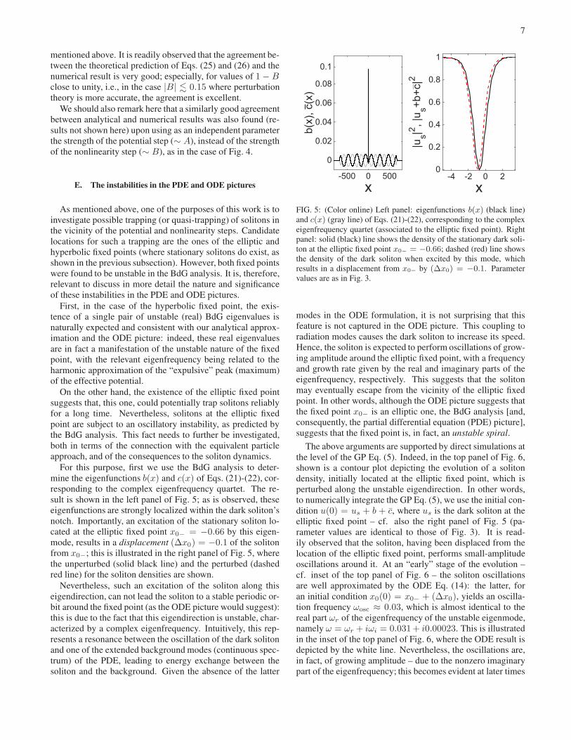
x-500 0 500

b(x

), c

(x)

0

0.02

0.04

0.06

0.08

0.1

x-4 -2 0 2

|us|2

,|u

s+

b+

c|2

0

0.2

0.4

0.6

0.8

1

FIG. 5: (Color online) Left panel: eigenfunctions b(x) (black line)

and c(x) (gray line) of Eqs. (21)-(22), corresponding to the complex

eigenfrequency quartet (associated to the elliptic fixed point). Right

panel: solid (black) line shows the density of the stationary dark soli-

ton at the elliptic fixed point x0− = −0.66; dashed (red) line shows

the density of the dark soliton when excited by this mode, which

results in a displacement from x0− by (∆x0) = −0.1. Parameter

values are as in Fig. 3.

modes in the ODE formulation, it is not surprising that this

feature is not captured in the ODE picture. This coupling to

radiation modes causes the dark soliton to increase its speed.

Hence, the soliton is expected to perform oscillations of grow-

ing amplitude around the elliptic fixed point, with a frequency

and growth rate given by the real and imaginary parts of the

eigenfrequency, respectively. This suggests that the soliton

may eventually escape from the vicinity of the elliptic fixed

point. In other words, although the ODE picture suggests that

the fixed point x0− is an elliptic one, the BdG analysis [and,

consequently, the partial differential equation (PDE) picture],

suggests that the fixed point is, in fact, an unstable spiral.

The above arguments are supported by direct simulations at

the level of the GP Eq. (5). Indeed, in the top panel of Fig. 6,

shown is a contour plot depicting the evolution of a soliton

density, initially located at the elliptic fixed point, which is

perturbed along the unstable eigendirection. In other words,

to numerically integrate the GP Eq. (5), we use the initial con-

dition u(0) = us + b + c, where us is the dark soliton at the

elliptic fixed point – cf. also the right panel of Fig. 5 (pa-

rameter values are identical to those of Fig. 3). It is read-

ily observed that the soliton, having been displaced from the

location of the elliptic fixed point, performs small-amplitude

oscillations around it. At an “early” stage of the evolution –

cf. inset of the top panel of Fig. 6 – the soliton oscillations

are well approximated by the ODE Eq. (14): the latter, for

an initial condition x0(0) = x0− + (∆x0), yields an oscilla-

tion frequency ωosc ≈ 0.03, which is almost identical to the

real part ωr of the eigenfrequency of the unstable eigenmode,

namely ω = ωr + iωi = 0.031+ i0.00023. This is illustrated

in the inset of the top panel of Fig. 6, where the ODE result is

depicted by the white line. Nevertheless, the oscillations are,

in fact, of growing amplitude – due to the nonzero imaginary

part of the eigenfrequency; this becomes evident at later times

8

t0 4000 8000 12000

x

-15

-10

-5

0

0

0.2

0.4

0.6

0.8

1

t0 900 1900

x

-2

0

2

0

0.5

1

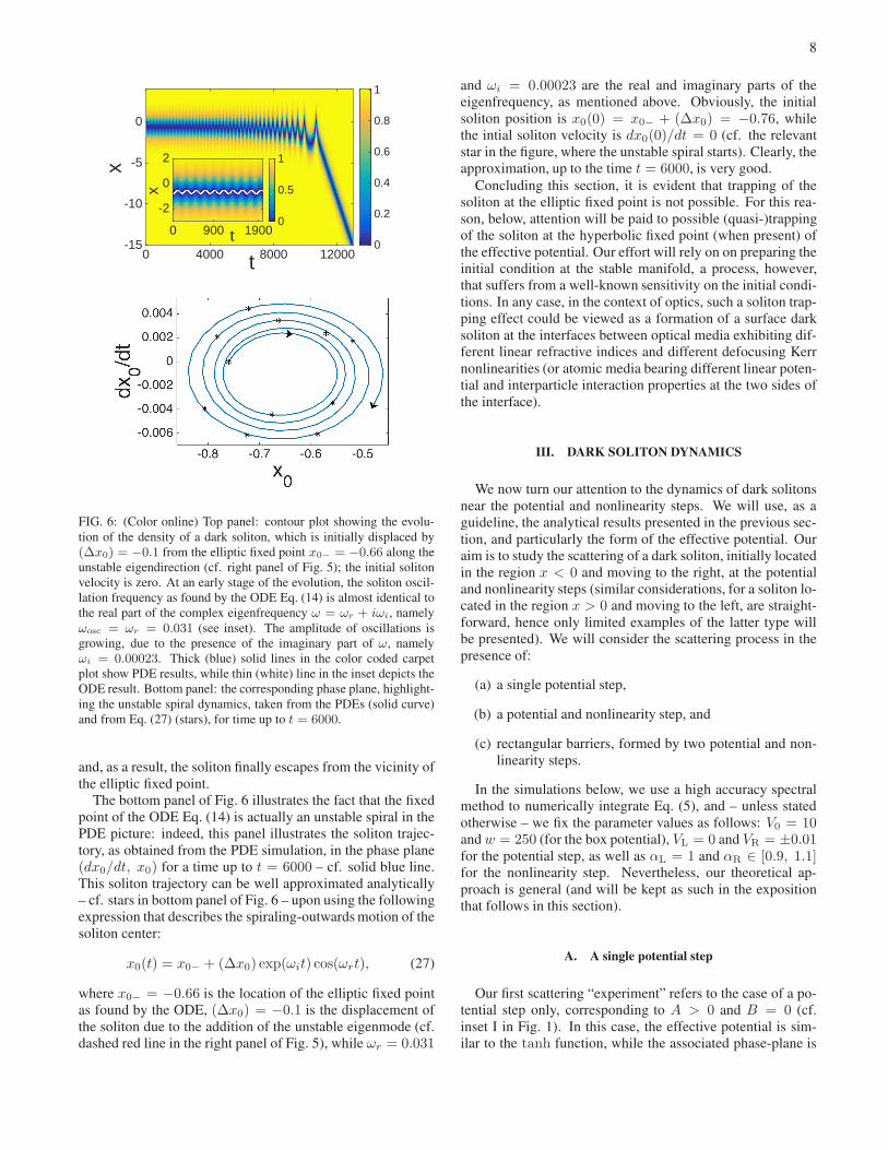
FIG. 6: (Color online) Top panel: contour plot showing the evolu-

tion of the density of a dark soliton, which is initially displaced by

(∆x0) = −0.1 from the elliptic fixed point x0− = −0.66 along the

unstable eigendirection (cf. right panel of Fig. 5); the initial soliton

velocity is zero. At an early stage of the evolution, the soliton oscil-

lation frequency as found by the ODE Eq. (14) is almost identical to

the real part of the complex eigenfrequency ω = ωr + iωi, namely

ωosc = ωr = 0.031 (see inset). The amplitude of oscillations is

growing, due to the presence of the imaginary part of ω, namely

ωi = 0.00023. Thick (blue) solid lines in the color coded carpet

plot show PDE results, while thin (white) line in the inset depicts the

ODE result. Bottom panel: the corresponding phase plane, highlight-

ing the unstable spiral dynamics, taken from the PDEs (solid curve)

and from Eq. (27) (stars), for time up to t = 6000.

and, as a result, the soliton finally escapes from the vicinity of

the elliptic fixed point.

The bottom panel of Fig. 6 illustrates the fact that the fixed

point of the ODE Eq. (14) is actually an unstable spiral in the

PDE picture: indeed, this panel illustrates the soliton trajec-

tory, as obtained from the PDE simulation, in the phase plane

(dx0/dt, x0) for a time up to t = 6000 – cf. solid blue line.

This soliton trajectory can be well approximated analytically

– cf. stars in bottom panel of Fig. 6 – upon using the following

expression that describes the spiraling-outwards motion of the

soliton center:

x0(t) = x0− + (∆x0) exp(ωit) cos(ωrt), (27)

where x0− = −0.66 is the location of the elliptic fixed point

as found by the ODE, (∆x0) = −0.1 is the displacement of

the soliton due to the addition of the unstable eigenmode (cf.

dashed red line in the right panel of Fig. 5), while ωr = 0.031

and ωi = 0.00023 are the real and imaginary parts of the

eigenfrequency, as mentioned above. Obviously, the initial

soliton position is x0(0) = x0− + (∆x0) = −0.76, while

the intial soliton velocity is dx0(0)/dt = 0 (cf. the relevant

star in the figure, where the unstable spiral starts). Clearly, the

approximation, up to the time t = 6000, is very good.

Concluding this section, it is evident that trapping of the

soliton at the elliptic fixed point is not possible. For this rea-

son, below, attention will be paid to possible (quasi-)trapping

of the soliton at the hyperbolic fixed point (when present) of

the effective potential. Our effort will rely on on preparing the

initial condition at the stable manifold, a process, however,

that suffers from a well-known sensitivity on the initial condi-

tions. In any case, in the context of optics, such a soliton trap-

ping effect could be viewed as a formation of a surface dark

soliton at the interfaces between optical media exhibiting dif-

ferent linear refractive indices and different defocusing Kerr

nonlinearities (or atomic media bearing different linear poten-

tial and interparticle interaction properties at the two sides of

the interface).

III. DARK SOLITON DYNAMICS

We now turn our attention to the dynamics of dark solitons

near the potential and nonlinearity steps. We will use, as a

guideline, the analytical results presented in the previous sec-

tion, and particularly the form of the effective potential. Our

aim is to study the scattering of a dark soliton, initially located

in the region x < 0 and moving to the right, at the potential

and nonlinearity steps (similar considerations, for a soliton lo-

cated in the region x > 0 and moving to the left, are straight-

forward, hence only limited examples of the latter type will

be presented). We will consider the scattering process in the

presence of:

(a) a single potential step,

(b) a potential and nonlinearity step, and

(c) rectangular barriers, formed by two potential and non-

linearity steps.

In the simulations below, we use a high accuracy spectral

method to numerically integrate Eq. (5), and – unless stated

otherwise – we fix the parameter values as follows: V0 = 10and w = 250 (for the box potential), VL = 0 and VR = ±0.01for the potential step, as well as αL = 1 and αR ∈ [0.9, 1.1]for the nonlinearity step. Nevertheless, our theoretical ap-

proach is general (and will be kept as such in the exposition

that follows in this section).

A. A single potential step

Our first scattering “experiment” refers to the case of a po-

tential step only, corresponding to A > 0 and B = 0 (cf.

inset I in Fig. 1). In this case, the effective potential is sim-

ilar to the tanh function, while the associated phase-plane is

9

W(x

0)

×10-3

-2-1012

x0

-5 -3 -1 0 1 3 5

dx0/d

t

-0.2

-0.1

0

0.1

-5

0.0960.1

(b)

(a)

AB

+

+

∆W

**

*

* * +

* + +

FIG. 7: (Color online) The case of a single potential step, A = 0.01and B = 0, corresponding to VL = 0, VR = 0.01, αR = αL, and

µL = 1. Top panel (a): effective potential W (x0); shown also is the

potential difference ∆W = W (+∞)− W (−∞) = 4.99 × 10−3.

Middle panel (b): corresponding phase plane; inset shows the initial

conditions (red squares A and B) for the trajectories corresponding

to reflection or transmission, while stars and pluses depict respective

PDE results. Bottom panels: contour plots showing the evolution

of the dark soliton density for the initial conditions depicted in the

middle panel, i.e., x0 = −5 and φ = 9.6 × 10−2 (left), or φ = 0.1(right); note that, here, φc = 0.099. Thick (blue) solid curves in

the color coded carpet plot show PDE results, while dashed (white)

curves depict ODE results.

shown in the middle panel of the same figure. Clearly, ac-

cording to the particle picture for the soliton of the previous

section, a dark soliton incident from the left towards the po-

tential step can either be reflected or transmitted: if the soliton

has a velocity v = dx0/dt, and thus a kinetic energy

K =1

2v2 =

1

2sin2 φ ≈ 1

2φ2, (28)

smaller (greater) than the effective potential step ∆W =W (+∞)−W (−∞), as shown in the top panel of Fig. 7, then

it will be reflected (transmitted). Notice the approximation

(sinφ ≈ φ) here which is applicable for low speeds/kinetic

energies. This consideration leads to φ < φc or φ > φc for

reflection or transmission, where the critical value φc of the

soliton phase angle is given by:

φc =√2∆W. (29)

In the numerical simulations we found that the threshold be-

tween the two cases is quite sharp and is accurately predicted

by Eq. (29). Indeed, consider the scenario shown in Fig. 7,

corresponding to parameter values VL = 0, VR = 0.01, αR =

αL and µL = 1. In this case, we find that ∆W = 4.99×10−3,

which leads to the critical value (for reflection/transmission)

of the soliton phase angle φc = 9.99 × 10−2. Then, for a

soliton initially placed at x0 = −5, and for initial velocities

corresponding to phase angles φ = 9.6 × 10−2 or φ = 0.1,

we observe reflection or transmission, respectively. The cor-

responding soliton trajectories are depicted both in the phase

plane (x0, dx0/dt) in the middle panel of Fig. 7 and in the

space-time contour plots showing the evolution of the soliton

density in the bottom panels of the same figure (see trajec-

tories A and B for reflection and transmission, respectively).

Note that stars and pluses in the middle panel correspond to

results obtained by direct numerical integration of the partial

differential equation (PDE), Eq. (5), while the (white) dashed

curves in the bottom panels depict results obtained by the

ODE, Eq. (14). Obviously, the agreement between theoreti-

cal predictions and numerical results is very good.

Here we should recall that in the case where the nonlinear-

ity step is also present (B 6= 0), and when B > −A (for

A > 0) or B < −A (for A < 0), the form of the effec-

tive potential is similar to the one shown in the top panel of

Fig. 7. In such cases, corresponding results (not shown here)

are qualitatively similar to the ones presented above.

B. A potential and a nonlinearity step

Next, we study the case where both a potential and a non-

linearity step are present (i.e., A,B 6= 0), and there exist fixed

points in the effective particle picture. One such case that

we consider in more detail below is the one corresponding to

A = 0.01 and B = −0.015 (respective parameter values are

VL = 0, VR = 0.01, αR/αL = 0.985, and µL = 1). Note that

for this choice the effective potential asymptotically vanishes,

as shown in the top panel of Fig. 8; nevertheless, results qual-

itatively similar to the ones that we present below can also be

obtained for nonvanishing asymptotics of W (x0).The form of the effective potential now suggests the exis-

tence of an elliptic and a hyperbolic fixed point, located at

x0 ≈ ∓0.65 respectively. In this case too, one can identify

an energy threshold ∆W , now defined as ∆W = W (x0+) −W (−∞) = W (x0+), needed to be overcome by the soliton

kinetic energy in order for the soliton to be transmitted (oth-

erwise, i.e., for K < ∆W , the soliton is reflected). Using

the above parameter values, we find that ∆W = 2.4 × 10−4

and, hence, according to Eq. (29), the critical phase angle for

transmission/reflection is φc ≈ 0.022. In the simulations,

we considered a soliton with initial position and phase angle

x0 = −5 and φ = 0.034 > φc, respectively (cf. point A in the

phase plane shown in the second panel of Fig. 8), and found

that, indeed, the soliton is transmitted through the effective

potential barrier of strength ∆W . The respective trajectory

(starting from point A) is shown in the second panel of Fig. 8.

Asterisks along this trajectory, as well as contour plot A in the

same figure, show PDE results obtained from direct numeri-

cal integration of Eq. (5); as in the case of Fig. 7, the (white)

dashed line corresponds to the ODE result.

To study the possibility of soliton trapping, we have also

10

t0 500 1000

x

-9

-5

0

5

9

0

0.5

1B

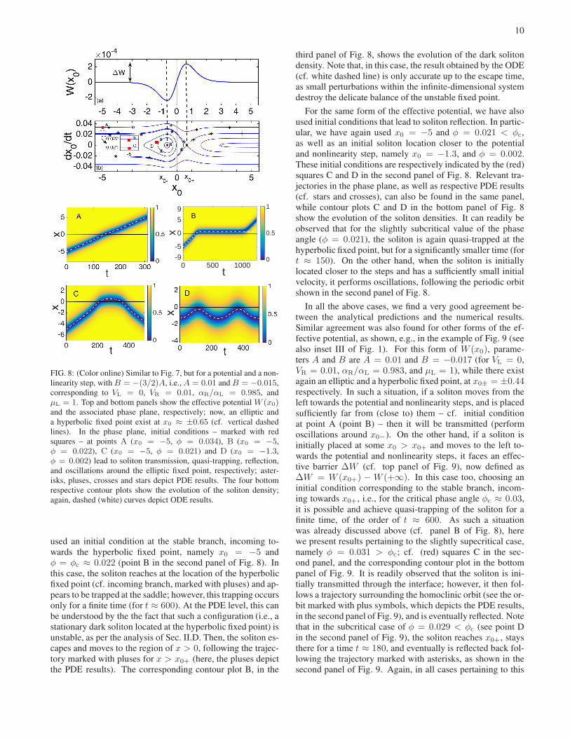
FIG. 8: (Color online) Similar to Fig. 7, but for a potential and a non-

linearity step, with B = −(3/2)A, i.e., A = 0.01 and B = −0.015,

corresponding to VL = 0, VR = 0.01, αR/αL = 0.985, and

µL = 1. Top and bottom panels show the effective potential W (x0)and the associated phase plane, respectively; now, an elliptic and

a hyperbolic fixed point exist at x0 ≈ ±0.65 (cf. vertical dashed

lines). In the phase plane, initial conditions – marked with red

squares – at points A (x0 = −5, φ = 0.034), B (x0 = −5,

φ = 0.022), C (x0 = −5, φ = 0.021) and D (x0 = −1.3,

φ = 0.002) lead to soliton transmission, quasi-trapping, reflection,

and oscillations around the elliptic fixed point, respectively; aster-

isks, pluses, crosses and stars depict PDE results. The four bottom

respective contour plots show the evolution of the soliton density;

again, dashed (white) curves depict ODE results.

used an initial condition at the stable branch, incoming to-

wards the hyperbolic fixed point, namely x0 = −5 and

φ = φc ≈ 0.022 (point B in the second panel of Fig. 8). In

this case, the soliton reaches at the location of the hyperbolic

fixed point (cf. incoming branch, marked with pluses) and ap-

pears to be trapped at the saddle; however, this trapping occurs

only for a finite time (for t ≈ 600). At the PDE level, this can

be understood by the the fact that such a configuration (i.e., a

stationary dark soliton located at the hyperbolic fixed point) is

unstable, as per the analysis of Sec. II.D. Then, the soliton es-

capes and moves to the region of x > 0, following the trajec-

tory marked with pluses for x > x0+ (here, the pluses depict

the PDE results). The corresponding contour plot B, in the

third panel of Fig. 8, shows the evolution of the dark soliton

density. Note that, in this case, the result obtained by the ODE

(cf. white dashed line) is only accurate up to the escape time,

as small perturbations within the infinite-dimensional system

destroy the delicate balance of the unstable fixed point.

For the same form of the effective potential, we have also

used initial conditions that lead to soliton reflection. In partic-

ular, we have again used x0 = −5 and φ = 0.021 < φc,

as well as an initial soliton location closer to the potential

and nonlinearity step, namely x0 = −1.3, and φ = 0.002.

These initial conditions are respectively indicated by the (red)

squares C and D in the second panel of Fig. 8. Relevant tra-

jectories in the phase plane, as well as respective PDE results

(cf. stars and crosses), can also be found in the same panel,

while contour plots C and D in the bottom panel of Fig. 8

show the evolution of the soliton densities. It can readily be

observed that for the slightly subcritical value of the phase

angle (φ = 0.021), the soliton is again quasi-trapped at the

hyperbolic fixed point, but for a significantly smaller time (for

t ≈ 150). On the other hand, when the soliton is initially

located closer to the steps and has a sufficiently small initial

velocity, it performs oscillations, following the periodic orbit

shown in the second panel of Fig. 8.

In all the above cases, we find a very good agreement be-

tween the analytical predictions and the numerical results.

Similar agreement was also found for other forms of the ef-

fective potential, as shown, e.g., in the example of Fig. 9 (see

also inset III of Fig. 1). For this form of W (x0), parame-

ters A and B are A = 0.01 and B = −0.017 (for VL = 0,

VR = 0.01, αR/αL = 0.983, and µL = 1), while there exist

again an elliptic and a hyperbolic fixed point, at x0± = ±0.44respectively. In such a situation, if a soliton moves from the

left towards the potential and nonlinearity steps, and is placed

sufficiently far from (close to) them – cf. initial condition

at point A (point B) – then it will be transmitted (perform

oscillations around x0−). On the other hand, if a soliton is

initially placed at some x0 > x0+ and moves to the left to-

wards the potential and nonlinearity steps, it faces an effec-

tive barrier ∆W (cf. top panel of Fig. 9), now defined as

∆W = W (x0+) − W (+∞). In this case too, choosing an

initial condition corresponding to the stable branch, incom-

ing towards x0+, i.e., for the critical phase angle φc ≈ 0.03,

it is possible and achieve quasi-trapping of the soliton for a

finite time, of the order of t ≈ 600. As such a situation

was already discussed above (cf. panel B of Fig. 8), here

we present results pertaining to the slightly supecritical case,

namely φ = 0.031 > φc; cf. (red) squares C in the sec-

ond panel, and the corresponding contour plot in the bottom

panel of Fig. 9. It is readily observed that the soliton is ini-

tially transmitted through the interface; however, it then fol-

lows a trajectory surrounding the homoclinic orbit (see the or-

bit marked with plus symbols, which depicts the PDE results,

in the second panel of Fig. 9), and is eventually reflected. Note

that in the subcritical case of φ = 0.029 < φc (see point D

in the second panel of Fig. 9), the soliton reaches x0+, stays

there for a time t ≈ 180, and eventually is reflected back fol-

lowing the trajectory marked with asterisks, as shown in the

second panel of Fig. 9. Again, in all cases pertaining to this

11

FIG. 9: (Color online) Similar to Fig. 8, for a potential and a nonlin-

earity step, but now for A = 0.01 and B = −0.017, corresponding

to VL = 0, VR = 0.01, αR/αL = 0.983, and µL = 1. The form

of W (x0) (top panel) suggests the existence of an elliptic and a hy-

perbolic fixed point, at x0± = ±0.44 (vertical dashed lines). In the

phase plane (second panel) shown are initial conditions, for a soli-

ton moving to the right, at points A (x0 = −5, φ = 0.005) and B

(x0 = −1, φ = 0.001), as well as for a soliton moving to the left,

at points C (x0 = 5, φ = 0.031 > φc ≈ 0.030) and D (x0 = 5,

φ = 0.029 < φc); in the relevant trajectories, stars, crosses, pluses,

and asterisks, respectively, denote PDE results. Corresponding con-

tour plots A, B, and C for the soliton density are shown in the bottom

panels, with the dashed white lines depicting ODE results.

form of W (x0), the agreement between the analytical predic-

tions and the numerical results is very good.

C. Rectangular barriers

Our analytical approximation can straightforwardly be ex-

tended to the case of multiple potential and nonlinearity steps.

Here, we will present results for such a case, where two steps,

located at x = −L and x = L, are combined so as to form

rectangular barriers, in both the linear potential and the non-

linearity of the system. In particular, we consider the follow-

ing profiles for the potential and the scattering length:

V (x) = Vb(x) +

{

VR, |x| > L

VL, |x| < L, (30)

α(x) =

{

αR, |x| > L

αL, |x| < L. (31)

In such a situation, the effective potential can be found fol-

lowing the lines of the analysis presented in Sec. II.B: taking

into regard that the perturbation P (υ) in Eq. (7) has now the

form:

P (υ) =(

A+B|υ|2)

υ [H(x + L)−H(x− L)] , (32)

it is straightforward to find that the relevant effective potential

is given by:

W (x0) =1

8

(

2A+B)

[tanh(L− x0) + tanh(L + x0)]

+1

24B[tanh3(L− x0) + tanh3(L+ x0)]. (33)

Typically, i.e., for sufficiently large arbitrary values of L,

the effective potential is as shown in the top panel of Fig. 10;

in this example, we used L = 5, while A = 0.01 and B =−0.015. It is readily observed that, in this case, the effective

potential takes the form of a superposition of the ones shown

in Fig. 8, which are now located at ±5. The associated phase

plane is shown in the middle panel of Fig. 10; shown also is an

initial condition (red square point A) corresponding to soliton

oscillations around the elliptic fixed point at the origin. The

corresponding soliton trajectory is depicted both in the phase

plane in the middle panel of Fig. 10 and in the space-time

contour plot showing the evolution of the soliton density in the

bottom panel of the same figure. Note that quasi-trapping of

the soliton is also possible in this case: indeed, we have found

that starting from the stable branch, at x0 = −8.6 and φ =2.2×10−2 (point A in the middle panel of Fig. 10), the soliton

is trapped at the hyperbolic fixed point at −4.34 for a time

t ≈ 600, and finally it is reflected back (see trajectory marked

with stars); the soliton trajectory in the space-time contour

plot is qualitatively similar to the one shown in the bottom left

panel of Fig. 7 (result not shown here). Once again, agreement

between theoretical predictions and numerical results for this

setting is very good as well.

An interesting situation occurs as L decreases. To better

illustrate what happens in this case, and also to make con-

nections with earlier work [12], we consider the simpler case

of B = 0 (i.e., the nonlinearity step is absent). Then, as-

suming that A = b/(2L) (with b being an arbitrary small

parameter), and in the limit of L → 0, the potential step

takes the form of a delta-like impurity of strength b. In this

case, the effective potential of Eq. (33) is reduced to the form

W (x0) = (b/4)sech2(x0). This result recovers the one re-

ported in Ref. [12] (see also Refs. [8, 13]), where the inter-

action of dark solitons with localized impurities was studied;

cf. Eq. (16) of that work, but in the absence of the trapping

potential Utr.

12

W(x

0)

×10-4

-2

-1

0

1

2

x0

-8 -6 -4 -2 0 2 4 6 8

dx0/d

t

-0.04

-0.02

0

0.02

0.04

(a)

*

*

+

(b)

** + +

FIG. 10: (Color online) The case of two potential and nonlinearity

steps forming respective rectangular barriers, for L = 5, A = 0.01and B = −0.015, corresponding to VL = 0, VR = 0.01, αR/αL =0.985, µL = 1. Top panel (a): the effective potential W (x0) – cf.

Eq. (33); dashed lines depict the elliptic fixed points at the origin

and at ±5.66, as well as a pair of hyperbolic fixed points at ±4.34.

Middle panel (b): the associated phase plane; (red) squares A and

B depict initial conditions corresponding to quasi-trapping (x0 =−8.6 and φ = 2.2 × 10−3) or oscillations (x0 = −3 and φ =3× 10−3), while stars pluses depict respective PDE results. Bottom

panel: contour plot showing the evolution of the dark soliton density

for the initial condition B depicted in the middle panel; as before,

dashed (white) line depict ODE results.

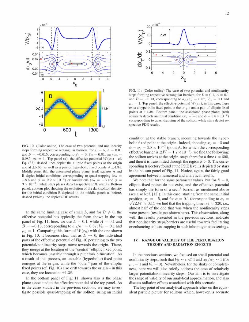
In the same limiting case of small L, and for B 6= 0, the

effective potential has typically the form shown in the top

panel of Fig. 11; here, we use L = 0.1, while A = 0.1 and

B = −0.13, corresponding to aR/aL = 0.87, VR = 0.1 and

µL = 1. Comparing this form of W (x0) with the one shown

in Fig. 10, it becomes clear that as L → 0, the individual

parts of the effective potential of Fig. 10 pertaining to the two

potential/nonlinearity steps move towards the origin. There,

they merge at the location of the “central” elliptic fixed point,

which becomes unstable through a pitchfork bifurcation. As

a result of this process, an unstable (hyperbolic) fixed point

emerges at the origin, while the “outer” pair of the elliptic

fixed points (cf. Fig. 10) also drift towards the origin – in this

case, they are located at ±1.38.

In the bottom panel of Fig. 11, shown also is the phase

plane associated to the effective potential of the top panel. As

in the cases studied in the previous sections, we may inves-

tigate possible quasi-trapping of the soliton, using an initial

W(x

0)

×10-4

0

10

20

x0

-6 -4 -2 0 2 4 6

dx0/d

t

-0.1

0

0.1* *

** * *

∆W

A

FIG. 11: (Color online) The case of two potential and nonlinearity

steps forming respective rectangular barriers, for L = 0.1, A = 0.1and B = −0.13, corresponding to aR/aL = 0.87, VR = 0.1 and

µL = 1. Top panel: the effective potential W (x0); in this case, there

exist a hyperbolic fixed point at the origin and a pair of elliptic fixed

points at ±1.38. Bottom panel: the associated phase plane; (red)

square A depicts an initial condition (x0 = −5 and φ = 5.8×10−2)

corresponding to quasi-trapping of the soliton, while stars depict re-

spective PDE results.

condition at the stable branch, incoming towards the hyper-

bolic fixed point at the origin. Indeed, choosing x0 = −5 and

φ = φc = 5.8 × 10−2 (point A, for which the corresponding

effective barrier is ∆W = 1.7×10−3), we find the following:

the soliton arrives at the origin, stays there for a time t ≈ 600,

and then it is transmitted through the region x > 0. The corre-

sponding trajectory found at the PDE level is depicted by stars

in the bottom panel of Fig. 11. Notice, again, the fairly good

agreement between numerical and analytical results.

We note that for the same parameter values, but for B = 0,

elliptic fixed points do not exist, and the effective potential

has simply the form of a sech2 barrier, as mentioned above

(see also Ref. [12]). In this case, starting from the same initial

position, x0 = −5, and for φ = 0.1 (corresponding to φc =√2∆W ≈ 0.1), we find that the trapping time is t ≈ 320, i.e.,

almost half of the one that was when the nonlinearity steps

were present (results not shown here). This observation, along

with the results presented in the previous sections, indicate

that nonlinearity steps/barriers are useful towards facilitating

or enhancing soliton trapping in such inhomogeneous settings.

IV. RANGE OF VALIDITY OF THE PERTURBATION

THEORY AND RADIATION EFFECTS

In the previous sections, we focused on small potential and

nonlinearity steps, such that VR ∼ ǫ ≪ 1 and αR/αL ∼ 1 (for

µL = 1 and VL = 0). Nevertheless, for the shake of complete-

ness, here we will also briefly address the case of relatively

larger potential/nonlinearity steps. Our aim is to investigate

the range of validity of our analytical approximation, and also

discuss radiation effects associated with this scenario.

The key point of our analytical approach relies on the equiv-

alent particle picture for solitons which, however, is accurate

13

only in the perturbative regime of small potential and nonlin-

earity steps. By increasing the amplitude of the latter, how-

ever, the soliton behaves more like a wave, rather than a par-

ticle: in fact, an incident soliton at such discontinuities, apart

from being either transmitted or reflected, emits radiation in

the form of sound waves. These sound waves propagate in

both regions x < 0 and x > 0, with the respective velocities

of sound, namely c(L)s = 1 for x < 0 and c

(R)s =

√nR for

x > 0 (where nR is the background density in this region).

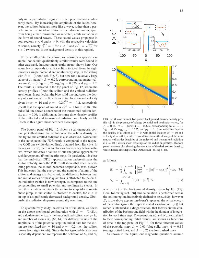
To better illustrate the above, we consider a specific ex-

ample; notice that qualitatively similar results were found in

other cases and, thus, pertinent results are not shown here. Our

example corresponds to a dark soliton incident from the right

towards a single potential and nonlinearity step, in the setting

with B = −(3/2)A (cf. Fig. 8), but now for a relatively large

value of A, namely A = 0.25; corresponding parameter val-

ues are VL = 0, VR = 0.25, αR/αL = 0.625, and µR = 1.2.

The result is illustrated in the top panel of Fig. 12, where the

density profiles of both the soliton and the emitted radiation

are shown. In particular, the blue solid line indicates the den-

sity of a soliton, at t = 0, with an initial location and velocity

given by x0 = 10 and φ = −0.2c(L)s = −0.2, respectively

(recall that the speed of sound is c(L)s = 1 for x < 0). The

red solid line shows a snapshot of the transmitted soliton den-

sity at t = 100; in addition, at the same time, density profiles

of the reflected and transmitted radiation are clearly visible

(insets in this figure show pertinent close ups).

The bottom panel of Fig. 12 shows a spatiotemporal con-

tour plot illustrating the evolution of the soliton density; in

this figure, the emitted radiation is also observed. Notice that

in the same panel, the PDE result is compared to the respec-

tive ODE one (white dashed line), obtained from Eq. (14). In

the region x < 0, there is an obvious discrepancy between the

two, which indicates a failure of our analytical approach for

such large potential/nonlinearity steps. In particular, it is clear

that the analytical (ODE) approximation underestimates the

soliton velocity, since the PDE result shows that after the scat-

tering process, the soliton becomes deeper and, thus, slower.

This indicates that the energy and the number of atoms of the

soliton and energy are decreased; the difference between final

and initial values of these quantities is attributed to the emit-

ted radiation (which is now stronger, as compared to the one

corresponding to small potential and nonlinearity steps). In

fact, this radiation facilitates the soliton to adapt (decrease) its

phase jump, as the soliton is “forced” to evolve, for x < 0,

on top of a significantly decreased background density. Obvi-

ously, the radiation disperses eventually over time.

To quantitatively study the emission of radiation, we focus

on the above mentioned configuration with B = −(3/2)A,

and calculate numerically the renormalized soliton energy Es

and number of atoms Ns [63, 64] for different values of the

amplitude A of the potential step; the initial data for the soli-

ton are kept fixed (x0 = 10 and φ = −0.2, i.e., the soliton

moves from right to left). Since the background density here

is spatially dependent, we rephrase the defintion of Es and Ns

x-100 -50 0 50 100

|u(x

,t)|2

0

0.5

1

1.5t=0t=100

40 60 801.16

1.18

1.2

1.22

-80 -70 -600.9

1

1.1

t0 30 60 90

x-10

0

10

0

0.2

0.4

0.6

0.8

1

1.2

FIG. 12: (Color online) Top panel: background density density pro-

file |u|2 in the presence of a large potential and nonlinearity step, for

A = 0.25, B = −(3/2)A = −0.375, corresponding to VL = 0,

VR = 0.25, αR/αL = 0.625, and µL = 1. Blue solid line depicts

the density of a soliton at t = 0, with initial location x0 = 10 and

velocity φ = −0.2, while red solid line shows the density of the soli-

ton, as well as the densities of the reflected and transmitted radiation

at t = 100; insets show close ups of the radiation profiles. Bottom

panel: contour plot showing the evolution of the dark soliton density;

white dashed line depicts the ODE result [cf. Eq. (14)].

as follows:

Es =1

2

∫ x0+2ξ

x0−2ξ

{

∣

∣

∣

∣

∂u

∂x

∣

∣

∣

∣

2

+[

|u|2 − n(x)]2

}

dx, (34)

Ns =

∫ x0+2ξ

x0−2ξ

[

n(x)− |u|2]

dx, (35)

where n(x) is the background density, given by Eq. (19).

Here, following Ref. [58], this calculation is performed across

the soliton region, indicatively defined to be x0±2ξ; however

Es in the above expression doesn’t represent the actual energy

of the soliton (given the explicit spatial variation of n(x)) but

rather is intended as a diagnostic tool that factors out the con-

tribution of the background field within the domain of integra-

tion for each time step. The quantities Es and Ns, normalized

to their corresponding initial values, are shown as functions

of time in the top panel of Fig. 13, for three different values

of the potential step: A = 0.01 (blue solid line), A = 0.15(orange dotted line), and A = 0.25 (yellow dashed line).

As shown in the figure, our diagnostic quantities assume

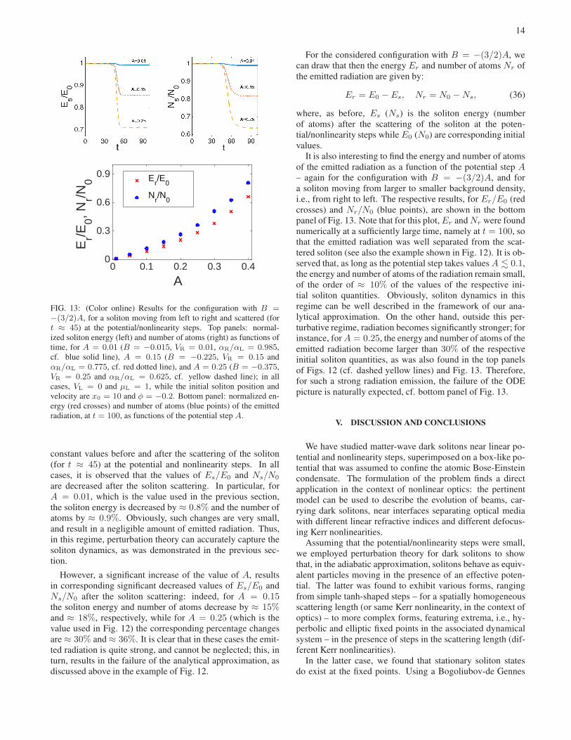
14

A0 0.1 0.2 0.3 0.4

Er/E

0, Nr/N

0

0

0.3

0.6

0.9 Er/E

0

Nr/N

0

FIG. 13: (Color online) Results for the configuration with B =−(3/2)A, for a soliton moving from left to right and scattered (for

t ≈ 45) at the potential/nonlinearity steps. Top panels: normal-

ized soliton energy (left) and number of atoms (right) as functions of

time, for A = 0.01 (B = −0.015, VR = 0.01, αR/αL = 0.985,

cf. blue solid line), A = 0.15 (B = −0.225, VR = 0.15 and

αR/αL = 0.775, cf. red dotted line), and A = 0.25 (B = −0.375,

VR = 0.25 and αR/αL = 0.625, cf. yellow dashed line); in all

cases, VL = 0 and µL = 1, while the initial soliton position and

velocity are x0 = 10 and φ = −0.2. Bottom panel: normalized en-

ergy (red crosses) and number of atoms (blue points) of the emitted

radiation, at t = 100, as functions of the potential step A.

constant values before and after the scattering of the soliton

(for t ≈ 45) at the potential and nonlinearity steps. In all

cases, it is observed that the values of Es/E0 and Ns/N0

are decreased after the soliton scattering. In particular, for

A = 0.01, which is the value used in the previous section,

the soliton energy is decreased by ≈ 0.8% and the number of

atoms by ≈ 0.9%. Obviously, such changes are very small,

and result in a negligible amount of emitted radiation. Thus,

in this regime, perturbation theory can accurately capture the

soliton dynamics, as was demonstrated in the previous sec-

tion.

However, a significant increase of the value of A, results

in corresponding significant decreased values of Es/E0 and

Ns/N0 after the soliton scattering: indeed, for A = 0.15the soliton energy and number of atoms decrease by ≈ 15%and ≈ 18%, respectively, while for A = 0.25 (which is the

value used in Fig. 12) the corresponding percentage changes

are ≈ 30% and ≈ 36%. It is clear that in these cases the emit-

ted radiation is quite strong, and cannot be neglected; this, in

turn, results in the failure of the analytical approximation, as

discussed above in the example of Fig. 12.

For the considered configuration with B = −(3/2)A, we

can draw that then the energy Er and number of atoms Nr of

the emitted radiation are given by:

Er = E0 − Es, Nr = N0 −Ns, (36)

where, as before, Es (Ns) is the soliton energy (number

of atoms) after the scattering of the soliton at the poten-

tial/nonlinearity steps while E0 (N0) are corresponding initial

values.

It is also interesting to find the energy and number of atoms

of the emitted radiation as a function of the potential step A– again for the configuration with B = −(3/2)A, and for

a soliton moving from larger to smaller background density,

i.e., from right to left. The respective results, for Er/E0 (red

crosses) and Nr/N0 (blue points), are shown in the bottom

panel of Fig. 13. Note that for this plot, Er and Nr were found

numerically at a sufficiently large time, namely at t = 100, so

that the emitted radiation was well separated from the scat-

tered soliton (see also the example shown in Fig. 12). It is ob-

served that, as long as the potential step takes values A . 0.1,

the energy and number of atoms of the radiation remain small,

of the order of ≈ 10% of the values of the respective ini-

tial soliton quantities. Obviously, soliton dynamics in this

regime can be well described in the framework of our ana-

lytical approximation. On the other hand, outside this per-

turbative regime, radiation becomes significantly stronger; for

instance, for A = 0.25, the energy and number of atoms of the

emitted radiation become larger than 30% of the respective

initial soliton quantities, as was also found in the top panels

of Figs. 12 (cf. dashed yellow lines) and Fig. 13. Therefore,

for such a strong radiation emission, the failure of the ODE

picture is naturally expected, cf. bottom panel of Fig. 13.

V. DISCUSSION AND CONCLUSIONS

We have studied matter-wave dark solitons near linear po-

tential and nonlinearity steps, superimposed on a box-like po-

tential that was assumed to confine the atomic Bose-Einstein

condensate. The formulation of the problem finds a direct

application in the context of nonlinear optics: the pertinent

model can be used to describe the evolution of beams, car-

rying dark solitons, near interfaces separating optical media

with different linear refractive indices and different defocus-

ing Kerr nonlinearities.

Assuming that the potential/nonlinearity steps were small,

we employed perturbation theory for dark solitons to show

that, in the adiabatic approximation, solitons behave as equiv-

alent particles moving in the presence of an effective poten-

tial. The latter was found to exhibit various forms, ranging

from simple tanh-shaped steps – for a spatially homogeneous

scattering length (or same Kerr nonlinearity, in the context of

optics) – to more complex forms, featuring extrema, i.e., hy-

perbolic and elliptic fixed points in the associated dynamical

system – in the presence of steps in the scattering length (dif-

ferent Kerr nonlinearities).

In the latter case, we found that stationary soliton states

do exist at the fixed points. Using a Bogoliubov-de Gennes

15

(BdG) analysis, we showed that these states are unstable: dark

solitons at the hyperbolic fixed points have a pair of unstable

real eigenvalues, while those at the elliptic fixed points have a

complex eigenfrequency quartet, dictating a purely exponen-

tial or an oscillatory instability, respectively. The case of the

oscillatory instability was studied in detail, and it was shown

that, in fact, the elliptic point in the effective particle picture

actually behaves as an unstable spiral in the framework of the

Gross-Pitaevskii model (and in accordance to the BdG analy-

sis). We also used an analytical approximation to determine

the real and imaginary parts of the relevant eigenfrequencies

as functions of the nonlinearity step strength. The analytical

predictions were found to be in good agreement with corre-

sponding numerical findings obtained in the framework of the

BdG analysis.

We then studied systematically soliton dynamics, for a vari-

ety of parameter values corresponding to all possible forms of

the effective potential. Adopting the aforementioned equiv-

alent particle picture, we found analytically necessary con-

ditions for soliton reflection at, or transmission through the

potential and nonlinearity steps: these correspond to initial

soliton velocities smaller or greater to the energy of the effec-

tive steps/barriers predicted by the perturbation theory and the

equivalent particle picture.

We also investigated the possibility of soliton (quasi-) trap-

ping, for initial conditions corresponding to the incoming, sta-

ble manifolds of the hyperbolic fixed points (which exist only

for inhomogeneous nonlinearities). In the context of optics,

such a trapping can be regarded as the formation of surface

dark solitons at the interface between dielectrics of different

refractive indices. We found that trapping is possible, but only

for a finite time. This effect can be understood by the fact that

stationary solitons at the hyperbolic fixed points are unstable,

as was corroborated by the BdG analysis. Thus small pertur-

bations (at the PDE level) eventually cause the departure of

the solitary wave from the relevant fixed points. Nevertheless,

it should be pointed out that the time of soliton quasi-trapping

was found to be of the order of 600√2ξ/cS in physical units;

thus, typically, for a healing length ξ of the order of a mi-

cron and a speed of sound cs of the order of a millimeter-

per-second, trapping time may be of the order of ≈ 850 ms.

This indicates that such a soliton quasi-trapping effect may

be observed in real experiments. Note that in all scenarios

(reflection, transmission, quasi-trapping) our analytical pre-

dictions were found to be in very good agreement with direct

numerical simulations in the framework of the original Gross-

Pitaevskii model.

We have also extended our considerations to study cases

involving two potential and nonlinearity steps, that are com-

bined so as to form corresponding rectangular barriers. Re-

flection, transmission and quasi-trapping of solitons in such

cases were studied too, again with a very good agreement be-

tween analytical and numerical results. In this setting, special

attention was paid to the limiting case of infinitesimally small

distance between the adjacent potential/nonlinearity steps that

form the barriers. In this case, we found that, due to a pitch-

fork bifurcation, the stability of the fixed point of the effective

potential at the barrier center changes: out of two hyperbolic

and one elliptic fixed point, a hyperbolic fixed point emerges,

and the potential rectangular barrier is reduced to a delta-like

impurity. The latter is described by a sech2 effective potential,

in accordance with the analysis of earlier works [8, 12, 13].

Finally, we also studied soliton scattering at relatively large

potential/nonlinearity steps. Our investigation reveals that, in

this case, soliton scattering results in significant emission of

radiation in both sides of the interface. We found that the soli-

ton’s number of atoms and energy decrease when the soliton

is scattered at regions of lower background density. The num-

ber of atoms and energy of the radiation was thus found to be

equal to the difference between initial and final values of the

soliton number of atoms and energy. We have also found that

our analytical approximation, based on the equivalent parti-

cle picture remains accurate as long as the percentage differ-

ence betwen potential/nonlinearity steps is up to 10%; in such

a case the radiation is actually negligible. Nevertheless, for

larger than 10% values, the emission of radiation is stronger;

this effect can not be captured by our analytical approach,

which evidently fails in such a nonperturbative regime.

Our methodology and results pose a number of interesting

questions for future studies. First, it would be interesting to

investigate how our perturbative results change as the poten-

tial/nonlinearity steps or barriers become larger, and/or attain

more realistic shapes (including steps bearing finite widths, as

well as Gaussian barriers – cf., e.g., recent work of Ref. [16]).

In the same context, a systematic numerical – and, possibly,

also analytical – study of the radiation of solitons during re-

flection or transmission (along the lines, e.g., of Ref. [58])

should also provide a more complete picture in this prob-

lem. Furthermore, a systematic study of settings involving

multiple such steps/barriers, and an investigation of the pos-

sibility of soliton trapping therein, would be particularly rele-

vant. In such settings, investigation of the dynamics of mov-

ing steps/barriers could find direct applications to fundamen-

tal studies relevant, e.g., to superfluidity (see, for instance,

Ref. [22]), transport of BECs [23], and even Hawking radia-

tion in analog black hole lasers implemented with BECs [68].

Finally, extension of our analysis to higher-dimensional set-

tings, would also be particularly challenging: first, in order

to investigate transverse excitation effects that are not cap-

tured within the quasi-1D setting, and second to study simi-

lar problems with vortices and other vortex structures. See,

e.g., Ref. [69] for a summary of relevant studies in higher-

dimensional settings, and Ref. [70] for a recent example of

manipulation/control of vortex patterns and their formation

via Gaussian barriers, motivated by experimentally accessible

laser beams.

Acknowledgments

The work of F.T. and D.J.F. was partially supported by

the Special Account for Research Grants of the University of

Athens. The work of F.T. and Z.A.A. was partially supported

by Qatar University under the scope of the Internal Grant

QUUG-CAS-DMSP-13/14-7. F.T. acknowledges hospitality

at Qatar University, where most of this work was carried out.

16

The work of P.G.K. at Los Alamos is partially supported by

the US Department of Energy. P.G.K. also gratefully acknowl-

edges the support of NSF-DMS-1312856, BSF-2010239, as

well as from the US-AFOSR under grant FA9550-12-1- 0332,

and the ERC under FP7, Marie Curie Actions, People, Inter-

national Research Staff Exchange Scheme (IRSES-605096).

The work of J.L.M. was supported in part by U.S. NSF Grants

DMS–1312874 and DMS-1352353.

[1] Yu. S. Kivshar and B. A. Malomed, Rev. Mod. Phys. 61, 763

(1989).

[2] I. M. Lifshitz and A. M. Kosevich, Rep. Prog. Phys. 29, 217

(1966).

[3] I. Ianni, S. L. Coz, and J. Royer, arXiv:1506.03761.

[4] A. M. Kosevich, Physica D 41, 253 (1990).

[5] X. D. Cao and B. A. Malomed, Phys. Lett. A 206, 177 (1995).

[6] R. H. Goodman, P. J. Holmes, and M. I. Weinstein, Physica D

192, 215 (2004).

[7] J. Holmer, J. Marzuola, and M. Zworski, Comm. Math. Phys.

274, 187 (2007); J. Holmer, J. Marzuola, and M. Zworski, J.

Nonlin. Sci. 17, 349 (2007).

[8] V. V. Konotop, V. M. Perez-Garcıa, Y.-F. Tang, and L. Vazquez,

Phys. Lett. A 236, 314 (1997).

[9] L. P. Pitaevskii and S. Stringari, Bose-Einstein Condensation

(Oxford University Press, Oxford, 2003).

[10] P. G. Kevrekidis, D. J. Frantzeskakis, and R. Carretero-

Gonzalez (eds.), Emergent Nonlinear Phenomena in

Bose-Einstein Condensates: Theory and Experiment

(Springer-Verlag, Berlin, 2008); R. Carretero-Gonzalez,

D. J. Frantzeskakis, and P. G. Kevrekidis, Nonlinearity 21, 139

(2008).

[11] V. S. Bagnato, D. J. Frantzeskakis, P. G. Kevrekidis, B. A. Mal-

omed and D. Mihalache, Rom. Rep. Phys. 67, 5 (2015).

[12] D. J. Frantzeskakis, G. Theocharis, F. K. Diakonos, P.

Schmelcher, and Yu. S. Kivshar, Phys. Rev. A 66, 053608

(2002).

[13] N. Bilas and N. Pavloff, Phys. Rev. A 72, 033618 (2005).

[14] N. Bilas and N. Pavloff, Phys. Rev. Lett. 95, 130403 (2005).

[15] G. Herring, P. G. Kevrekidis, R. Carretero-Gonzalez, B. A. Mal-

omed, D. J. Frantzeskakis, and A. R. Bishop, Phys. Lett. A 345,

144 (2005).

[16] I. Hans, J. Stockhofe, and P. Schmelcher, Phys. Rev. A 92,

013627 (2015).

[17] T. Ernst and J. Brand, Phys. Rev. A 81, 033614 (2010).

[18] C. Lee and J. Brand, Europhys. Lett. 73, 321 (2006).

[19] J. L. Helm, T. P. Billam, and S. A. Gardiner, Phys. Rev. A 85,

053621 (2012).

[20] A. D. Martin and J. Ruostekoski, New J. Phys. 14, 043040

(2012).

[21] Y. Nogami and F. M. Toyama, Phys. Lett. A 184, 245-250

(1994).

[22] P. Engels and C. Atherton, Phys. Rev. Lett. 99, 160405 (2007).

[23] D. Dries, S. E. Pollack, J. M. Hitchcock, and R. G. Hulet, Phys.

Rev. A 82, 033603 (2010).

[24] J. Cuevas, P. G. Kevrekidis, B. A. Malomed, P. Dyke, and R. G.

Hulet, New J. Phys. 15, 063006 (2013).

[25] A. L. Marchant, T. P. Billam, T. P. Wiles, M. M. H. Yu, S. A.

Gardiner, and S. L. Cornish, Nat. Com. 4, 1865 (2013).

[26] V. Achilleos, P. G. Kevrekidis, V. M. Rothos, and D. J.

Frantzeskakis, Phys. Rev. A 84, 053626 (2011).

[27] A. Alvarez, J. Cuevas, F. R. Romero, C. Hamner, J. J. Chang,

P. Engels, P. G. Kevrekidis, and D. J. Frantzeskakis, J. Phys. B:

At. Mol. Opt. Phys. 46, 065302 (2013).

[28] G. Theocharis, P. Schmelcher, P. G. Kevrekidis, and D. J.

Frantzeskakis, Phys. Rev. A 72, 033614 (2005).

[29] S. Middelkamp, P. G. Kevrekidis, D. J. Frantzeskakis and P.

Schmelcher, Phys. Lett. A 373, 262268 (2009).

[30] Y. V. Kartashov, B. A. Malomed, and L. Torner, Rev. Mod.

Phys. 83, 247 (2011).

[31] F. Kh. Abdullaev and M. Salerno, J. Phys. B: At. Mol. Opt.

Phys. 36, 2851 (2003).

[32] M. I. Rodas-Verde, H. Michinel, and V. M. Perez-Garcıa, Phys.

Rev. Lett. 95, 153903 (2005); A. V. Carpentier, H. Michinel,

M. I. Rodas-Verde, and V. M. Perez-Garcıa, Phys. Rev. A 74,

013619 (2006).

[33] F. Tsitoura, P. Kruger, P. G. Kevrekidis, and D. J. Frantzeskakis,

Phys. Rev. A, 91, 033633 (2015).

[34] G. Theocharis, P. Schmelcher, P. G. Kevrekidis, and D. J.

Frantzeskakis, Phys. Rev. A 74, 053614 (2006); J. Garnier

and F. Kh. Abdullaev, ibid. 74, 013604 (2006); P. Niarchou,

G. Theocharis, P. G. Kevrekidis, P. Schmelcher, and D. J.

Frantzeskakis, ibid. 76, 023615 (2007).

[35] C. Wang, K.J.H. Law, P. G. Kevrekidis, and M. A. Porter, Phys.

Rev. A 87, 023621 (2013).

[36] G. Dong, B. Hu, and W. Lu, Phys. Rev. A 74, 063601 (2006).

[37] H. Sakaguchi and B. A. Malomed, Phys. Rev. A 81, 013624

(2010);

[38] S. Holmes, M. A. Porter, P. Kruger, and P. G. Kevrekidis, Phys.

Rev. A 88, 033627 (2013).

[39] M. Kurzke, J.L. Marzuola and D. Spirn, preprint

arXiv:1510.08093 (2015).

[40] K. Hizanidis, Y. Kominis, and N. K. Efremidis, Opt. Express

16, 18296 (2008).

[41] R. Marangell, C.K.R.T. Jones, and H. Susanto, Nonlinearity 23,

2059 (2010).

[42] R. Marangell, H. Susanto, and C.K.R.T. Jones, J. Diff. Eq. 253,

1191 (2012).

[43] C. Wang, P. G. Kevrekidis, T. P. Horikis, and D. J.

Frantzeskakis, Phys. Lett. A 374, 3863 (2010); T. Mithun, K.

Porsezian, and B. Dey, Phys. Rev. E 88, 012904 (2013).

[44] F. Pinsker, N. G. Berloff, and V. M. Perez-Garcıa, Phys. Rev. A

87, 053624 (2013).

[45] A. Balaz, R. Paun, A. I. Nicolin, S. Balasubramanian, and R.

Ramaswamy, Phys. Rev. A 89, 023609 (2014).

[46] T. Kaneda and H. Saito, Phys. Rev. A 90, 053632 (2014).

[47] A. Weller, J. P. Ronzheimer, C. Gross, J. Esteve, M. K.

Oberthaler, D. J. Frantzeskakis, G. Theocharis, and P. G.

Kevrekidis, Phys. Rev. Lett. 101, 130401 (2008); S. Stellmer,

P. Soltan-Panahi, S. Dorscher, M. Baumert, E.-M. Richter, J.

Kronjager, K. Bongs, and K. Sengstock, Nat. Phys. 4, 496

(2008); S. Stellmer, C. Becker, P. Soltan-Panahi, E.-M. Richter,

S. Dorscher, M. Baumert, J. Kronjager, K. Bongs, and K. Sen-

gstock, Phys. Rev. Lett. 101, 120406 (2008); G. Theocharis,

A. Weller, J. P. Ronzheimer, C. Gross, M. K. Oberthaler, P. G.

Kevrekidis, and D. J. Frantzeskakis, Phys. Rev. A 81, 063604

(2010).

[48] B. T. Seaman, L. D. Carr, and M. J. Holland, Phys. Rev. A, 71,

033609 (2005).

[49] L. D. Carr, R. R. Miller, D. R. Bolton, and S. A. Strong, Phys.

17

Rev. A 86, 023621 (2012).

[50] S. Inouye, M. R. Andrews, J. Stenger, H. J. Miesner, D. M.

Stamper-Kurn, and W. Ketterle, Nature (London) 392, 151

(1998); J. Stenger, S. Inouye, M. R. Andrews, H.-J. Miesner, D.

M. Stamper-Kurn, and W. Ketterle, Phys. Rev. Lett. 82, 2422

(1999); J. L. Roberts, N. R. Claussen, J. P. Burke, Jr., C. H.

Greene, E. A. Cornell, and C. E.Wieman, ibid. 81, 5109 (1998);

S. L. Cornish, N. R. Claussen, J. L. Roberts, E. A. Cornell, and

C. E. Wieman, ibid. 85, 1795 (2000).

[51] F. K. Fatemi, K. M. Jones, and P. D. Lett, Phys. Rev. Lett. 85,

4462 (2000); M. Theis, G. Thalhammer, K. Winkler, M. Hell-

wig, G. Ruff, R. Grimm, and J. H. Denschlag, ibid. 93, 123001

(2004).

[52] A. C. Newell and J. V. Moloney, Nonlinear Optics (Addison-

Wesley, Redwood City, CA, 1992).

[53] A. B. Aceves, J. V. Moloney, and A. C. Newell, J. Opt. Soc.

Am. B 5, 559 (1988); Phys. Lett. A 129, 231 (1988); Phys. Rev.

A 39, 1809 (1989); ibid. 39, 1828 (1989).

[54] Yu. S. Kivshar, A. M. Kosevich, and O. A. Chubykalo, Phys.

Rev. A 41, 1677 (1990).

[55] Yu. S. Kivshar and M. L. Quiroga-Texeiro, Phys. Rev. A 48,

4750 (1993).

[56] Y. Kominis and K. Hizanidis, Phys. Rev. Lett. 102, 133903

(2009).

[57] H. Sakaguchi and M. Tamura, J. Phys. Soc. Jpn. 74, 292 (2005).

[58] N. G. Parker, N. P. Proukakis, M. Leadbeater, and C. S. Adams,

J. Phys. B: At. Mol. Opt. Phys. 36, 2891 (2003); N. G. Parker,

N. P. Proukakis, C. F. Barenghi, and C. S. Adams, J. Phys. B:

At. Mol. Opt. Phys. 37, S175 (2004).

[59] N. P. Proukakis, N. G. Parker, D. J. Frantzeskakis, and C. S.

Adams, J. Opt. B: Quantum Semiclass. Opt. 6, S380 (2004).

[60] H. Sakaguchi, Laser Phys. 16, 340 (2006).

[61] R. Folman, P. Kruger, J. Denschlag, J. Schmiedmayer, and C.

Henkel, Adv. At. Mol. Opt. Phys. 48, 263 (2002).

[62] L. D. Carr, C. W. Clark, and W. P. Reinhardt, Phys. Rev. A 62,

063610 (2000).

[63] Yu. S. Kivshar and X. Yang, Phys. Rev. E 49, 1657 (1994).

[64] D. J. Frantzeskakis, J. Phys. A: Math. Theor. 43, 213001 (2010).

[65] M. J. Ablowitz, S. D. Nixon, T. P. Horikis, and D. J.

Frantzeskakis, Proc. R. Soc. A 2133, 2597 (2011).

[66] D. E. Pelinovsky and P. G. Kevrekidis, ZAMP 59, 559 (2008).

[67] A. S. Rodrigues, P. G. Kevrekidis, M. A. Porter, D. J.

Frantzeskakis, P. Schmelcher, and A. R. Bishop, Phys. Rev. A

78, 013611 (2008).

[68] J. Steinhauer, Nat. Phys. 10, 864 (2014).

[69] P. G. Kevrekidis, D. J. Frantzeskakis, and R. Carretero-

Gonzalez, The defocusing Nonlinear Schrodinger Equation:

From Dark Solitons to Vortices and Vortex Rings (SIAM,

Philadelphia, 2015).

[70] B. Gertjerenken, P. G. Kevrekidis, R. Carretero-Gonzalez, and

B. P. Anderson, Phys. Rev. A 93, 023604 (2016).