DARK MATTERLECTURE NOTES

Lecture notes are largely based on a lectures series givenby Neil Weiner at PITP on dark matter

Notes Written by: JEFF ASAF DROR

2014

1

Contents

1 Preface 2

2 Introduction 2

3 What we know about DM 5

4 Models of dark matter 9

5 Forming DM 95.1 Canonical example 1: oscillating scalar field . . . . . . . . . . . . . . . . 10

6 Thermal dark matter candidates 13

7 Canonical WIMP 157.1 Neutralino . . . . . . . . . . . . . . . . . . . . . . . . . . . . . . . . . . . 17

8 Anomalies 178.1 Indirect detection . . . . . . . . . . . . . . . . . . . . . . . . . . . . . . . 18

8.1.1 Fermi line . . . . . . . . . . . . . . . . . . . . . . . . . . . . . . . 188.1.2 Fermi bump . . . . . . . . . . . . . . . . . . . . . . . . . . . . . . 198.1.3 Dark force models . . . . . . . . . . . . . . . . . . . . . . . . . . . 198.1.4 PAMELA and AMS . . . . . . . . . . . . . . . . . . . . . . . . . 20

8.2 Direct detection . . . . . . . . . . . . . . . . . . . . . . . . . . . . . . . . 218.2.1 DAMA . . . . . . . . . . . . . . . . . . . . . . . . . . . . . . . . . 218.2.2 CoGeNT . . . . . . . . . . . . . . . . . . . . . . . . . . . . . . . . 228.2.3 CRESST . . . . . . . . . . . . . . . . . . . . . . . . . . . . . . . . 228.2.4 CDMS-Si . . . . . . . . . . . . . . . . . . . . . . . . . . . . . . . 22

8.3 What can we conclude? . . . . . . . . . . . . . . . . . . . . . . . . . . . . 22

1 Preface

This lecture notes are based on a PITP course given by Neil Weiner . If you have anycorrections please let me know at ajd268@cornell.edu.

2 Introduction

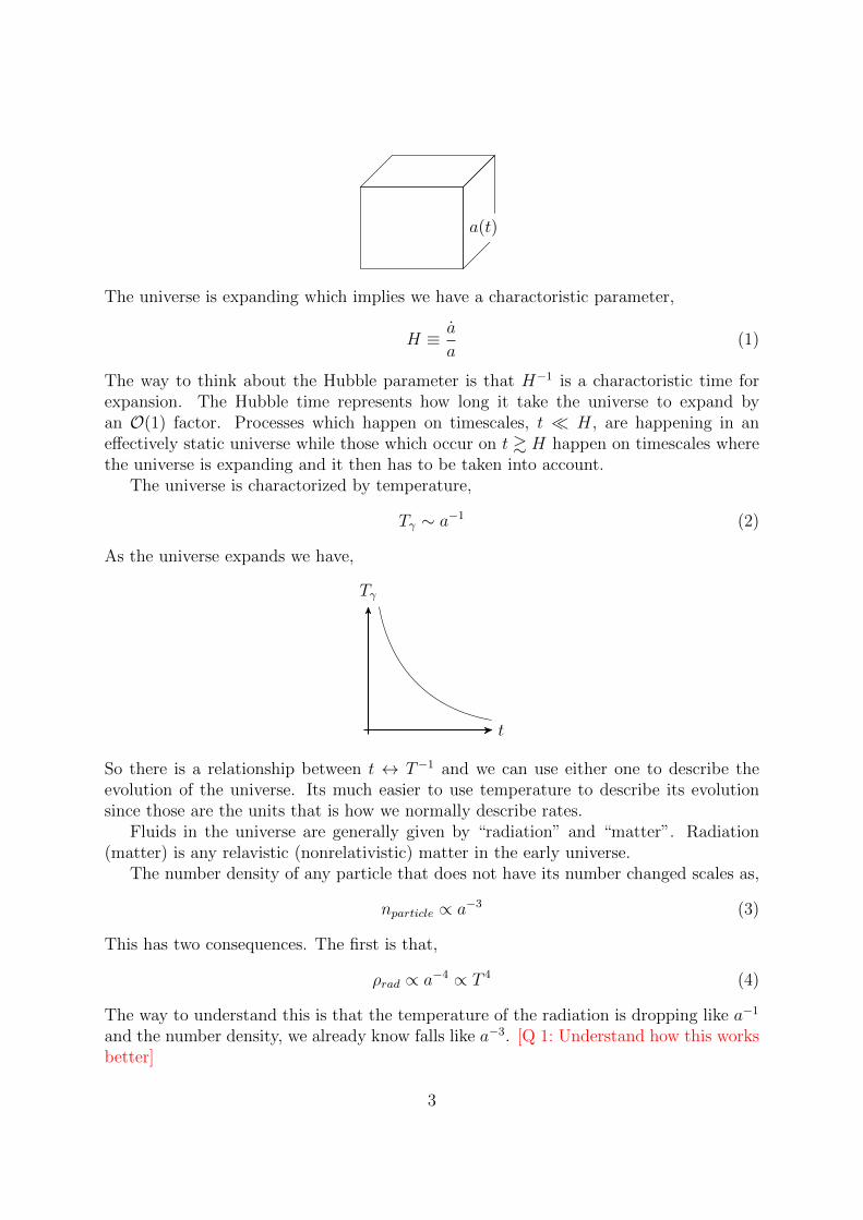
The universe is charactorized by a scale factor, a(t). The way we imagine this is we havesome box of the universe,

2

a(t)

The universe is expanding which implies we have a charactoristic parameter,

H ≡ a

a(1)

The way to think about the Hubble parameter is that H−1 is a charactoristic time forexpansion. The Hubble time represents how long it take the universe to expand byan O(1) factor. Processes which happen on timescales, t H, are happening in aneffectively static universe while those which occur on t & H happen on timescales wherethe universe is expanding and it then has to be taken into account.

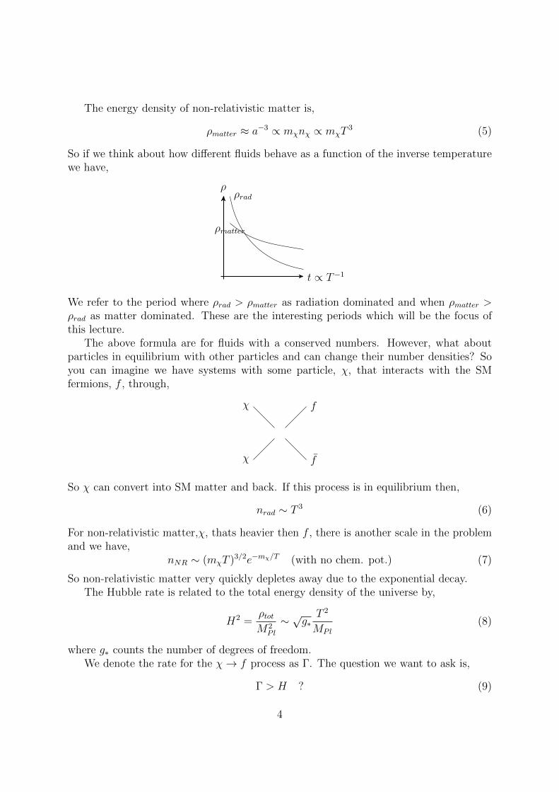
The universe is charactorized by temperature,

Tγ ∼ a−1 (2)

As the universe expands we have,

Tγ

t

So there is a relationship between t ↔ T−1 and we can use either one to describe theevolution of the universe. Its much easier to use temperature to describe its evolutionsince those are the units that is how we normally describe rates.

Fluids in the universe are generally given by “radiation” and “matter”. Radiation(matter) is any relavistic (nonrelativistic) matter in the early universe.

The number density of any particle that does not have its number changed scales as,

nparticle ∝ a−3 (3)

This has two consequences. The first is that,

ρrad ∝ a−4 ∝ T 4 (4)

The way to understand this is that the temperature of the radiation is dropping like a−1

and the number density, we already know falls like a−3. [Q 1: Understand how this worksbetter]

3

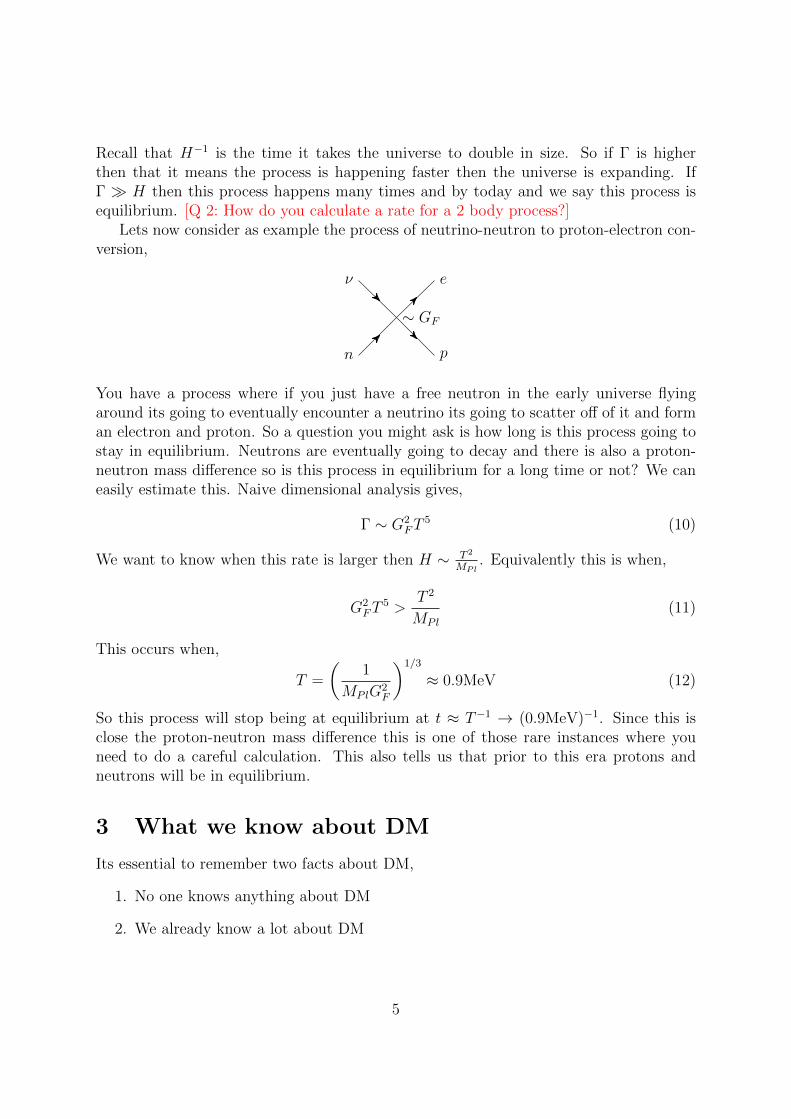
The energy density of non-relativistic matter is,

ρmatter ≈ a−3 ∝ mχnχ ∝ mχT3 (5)

So if we think about how different fluids behave as a function of the inverse temperaturewe have,

ρ

t ∝ T−1

ρrad

ρmatter

We refer to the period where ρrad > ρmatter as radiation dominated and when ρmatter >ρrad as matter dominated. These are the interesting periods which will be the focus ofthis lecture.

The above formula are for fluids with a conserved numbers. However, what aboutparticles in equilibrium with other particles and can change their number densities? Soyou can imagine we have systems with some particle, χ, that interacts with the SMfermions, f , through,

χ

χ f

f

So χ can convert into SM matter and back. If this process is in equilibrium then,

nrad ∼ T 3 (6)

For non-relativistic matter,χ, thats heavier then f , there is another scale in the problemand we have,

nNR ∼ (mχT )3/2e−mχ/T (with no chem. pot.) (7)

So non-relativistic matter very quickly depletes away due to the exponential decay.The Hubble rate is related to the total energy density of the universe by,

H2 =ρtotM2

Pl

∼ √g∗T 2

MPl

(8)

where g∗ counts the number of degrees of freedom.We denote the rate for the χ→ f process as Γ. The question we want to ask is,

Γ > H ? (9)

4

Recall that H−1 is the time it takes the universe to double in size. So if Γ is higherthen that it means the process is happening faster then the universe is expanding. IfΓ H then this process happens many times and by today and we say this process isequilibrium. [Q 2: How do you calculate a rate for a 2 body process?]

Lets now consider as example the process of neutrino-neutron to proton-electron con-version,

n

ν e

p

∼ GF

You have a process where if you just have a free neutron in the early universe flyingaround its going to eventually encounter a neutrino its going to scatter off of it and forman electron and proton. So a question you might ask is how long is this process going tostay in equilibrium. Neutrons are eventually going to decay and there is also a proton-neutron mass difference so is this process in equilibrium for a long time or not? We caneasily estimate this. Naive dimensional analysis gives,

Γ ∼ G2FT

5 (10)

We want to know when this rate is larger then H ∼ T 2

MPl. Equivalently this is when,

G2FT

5 >T 2

MPl

(11)

This occurs when,

T =

(1

MPlG2F

)1/3

≈ 0.9MeV (12)

So this process will stop being at equilibrium at t ≈ T−1 → (0.9MeV)−1. Since this isclose the proton-neutron mass difference this is one of those rare instances where youneed to do a careful calculation. This also tells us that prior to this era protons andneutrons will be in equilibrium.

3 What we know about DM

Its essential to remember two facts about DM,

1. No one knows anything about DM

2. We already know a lot about DM

5

These two should be kept in mind whenever discussing DM. Point 1 refers theoreticallyto how a normaly DM candidate should act. Point 2 is experimentally how much weknow from cosmilogical constraints. If we make a chart of what people have though overthe course of time,

Time Candidate< 1930 none

70’s-80’s Baryonic material (gas, unegnited stars, ...)80’s - 90’s Neutrinos

90’s < Neutralinos/axions

We write it in this form to emphasize that what a reasonable model of DM is changesover time and we shouldn’t be prejudice toward one form or another.

There are five most importantant pieces of evidence for DM,

1. Galaxies in clusters

• Galaxies cluster together. We can see how galaxies are moving and by theirvelocity distributions we can predict how much matter is luminous.

2. Rotational curves

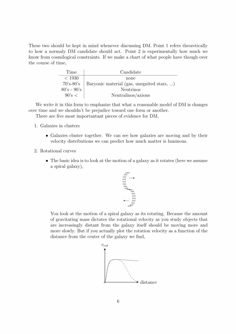
• The basic idea is to look at the motion of a galaxy as it rotates (here we assumea spiral galaxy),

You look at the motion of a spiral galaxy as its rotating. Because the amountof gravitating mass dictates the rotational velocity as you study objects thatare increasingly distant from the galaxy itself should be moving more andmore slowly. But if you actually plot the rotation velocity as a function of thedistance from the center of the galaxy we find,

vrot

distance

6

where the dashed line is the expected distribution and the solid line is whatis found in practice. These are known as “rotational curves”. We say that wehave flat rotation curves.

This is an important observation because its telling you that we have massout there that we can’t see but also that the mass is distributed in a differentfashion from ordinary matter. If we just had extra mass but still of the sametype then we would have a different normalization of the curves above but nota different distribution. We can conclude that there is mass far away from thecenter pulling the objects. This is referred to as the halo of the galaxy.

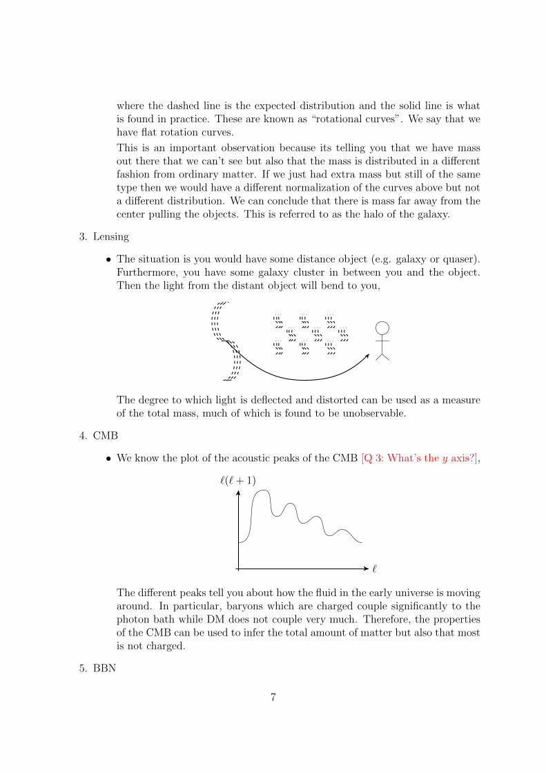
3. Lensing

• The situation is you would have some distance object (e.g. galaxy or quaser).Furthermore, you have some galaxy cluster in between you and the object.Then the light from the distant object will bend to you,

The degree to which light is deflected and distorted can be used as a measureof the total mass, much of which is found to be unobservable.

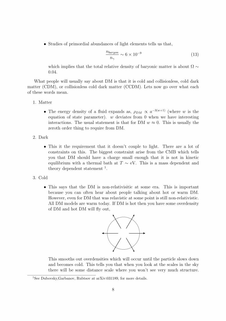
4. CMB

• We know the plot of the acoustic peaks of the CMB [Q 3: What’s the y axis?],

`(`+ 1)

`

The different peaks tell you about how the fluid in the early universe is movingaround. In particular, baryons which are charged couple significantly to thephoton bath while DM does not couple very much. Therefore, the propertiesof the CMB can be used to infer the total amount of matter but also that mostis not charged.

5. BBN

7

• Studies of primordial abundances of light elements tells us that,

nbaryonnγ

∼ 6× 10−9 (13)

which implies that the total relative density of baryonic matter is about Ω ∼0.04.

What people will usually say about DM is that it is cold and collisionless, cold darkmatter (CDM), or collisionless cold dark matter (CCDM). Lets now go over what eachof these words mean.

1. Matter

• The energy density of a fluid expands as, ρDM ∝ a−3(w+1) (where w is theequation of state parameter). w deviates from 0 when we have interestinginteractions. The usual statement is that for DM w ≈ 0. This is usually thezeroth order thing to require from DM.

2. Dark

• This it the requirement that it doesn’t couple to light. There are a lot ofconstraints on this. The biggest constraint arise from the CMB which tellsyou that DM should have a charge small enough that it is not in kineticequilibrium with a thermal bath at T ∼ eV. This is a mass dependent andtheory dependent statement 1.

3. Cold

• This says that the DM is non-relativisitic at some era. This is importantbecause you can often hear about people talking about hot or warm DM.However, even for DM that was relavistic at some point is still non-relativistic.All DM models are warm today. If DM is hot then you have some overdensityof DM and hot DM will fly out,

This smooths out overdensities which will occur until the particle slows downand becomes cold. This tells you that when you look at the scales in the skythere will be some distance scale where you won’t see very much structure.

1See Dubovsky,Garbanov, Rubtsov at arXiv:031189, for more details.

8

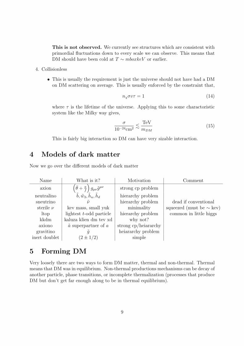
This is not observed. We currently see structures which are consistent withprimordial fluctuations down to every scale we can observe. This means thatDM should have been cold at T ∼ mboxkeV or earlier.

4. Collisionless

• This is usually the requirement is just the universe should not have had a DMon DM scattering on average. This is usually enforced by the constraint that,

nχσvτ = 1 (14)

where τ is the lifetime of the universe. Applying this to some charactoristicsystem like the Milky way gives,

σ

10−24cm2.

TeV

mDM

(15)

This is fairly big interaction so DM can have very sizable interaction.

4 Models of dark matter

Now we go over the different models of dark matter

Name What is it? Motivation Comment

axion(θ + a

f

)gµν g

µν strong cp problem

neutralino b, w3, hu, hd hierarchy problemsneutrino ν hierarchy problem dead if conventionalsterile ν kev mass, small yuk minimality squeezed (must be ∼ kev)

ltop lightest t-odd particle hierarchy problem common in little higgskkdm kaluza klien dm tev xd why not?axiono a superpartner of a strong cp/heiararchy

gravitino g heiararchy probleminert doublet (2± 1/2) simple

5 Forming DM

Very loosely there are two ways to form DM matter, thermal and non-thermal. Thermalmeans that DM was in equilibrium. Non-thermal productions mechanisms can be decay ofanother particle, phase transitions, or incomplete thermalization (processes that produceDM but don’t get far enough along to be in thermal equilibrium).

9

5.1 Canonical example 1: oscillating scalar field

Consider the Klien Gordan equation for homogenous field in the expanding universe,

φ+ 3Hφ+m2φ = 0 (16)

[Q 4: Show this.] For our purposes we take H to constant. That’s not actually the casein our universe but it doesn’t change the results we discuss here.

We can solve the differential equation by guessing, φ = φ0eωt. Inserting into the above

we have,ω2 + 3ωH +m2 = 0 (17)

which has the solutions,

ω =−3H ±

√9H2 − 4m2

2(18)

We can then take the limiting cases.For m H we have two solutions [Q 5: check],

ω = −3H,−2m2

3H(19)

The total energy density of this field is2,

ρ ∼ φ2 +m2φ2 (20)

For ω = −3H the energy density scales as,

ρ ∝ e−6Ht ∼ a−6 (21)

where we used the fact that for H = const, a ∼ eHt. So for the first solution the energydensity decays extremely rapidly. For the second solution we find,

φ2 ∼ m2 exp

(−2m2

3H

)(22)

but by assumption, m H, so,

φ2 ∼ m2 → const (23)

So if you have a mass much lighter then H then we have a part thats just going to sitthere and not do anything.

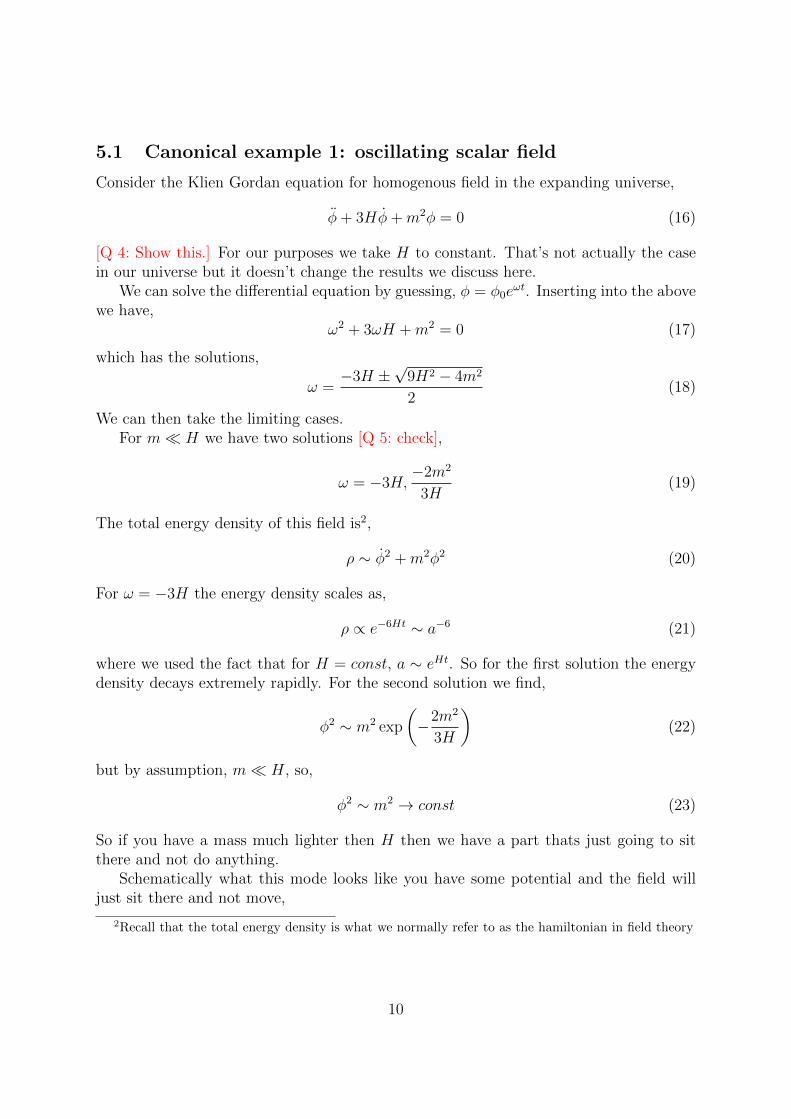
Schematically what this mode looks like you have some potential and the field willjust sit there and not move,

2Recall that the total energy density is what we normally refer to as the hamiltonian in field theory

10

Now lets consider the opposite limit, m H. Then the solutions are,

ω = −3H

2± im (24)

The energy density goes as,ρ ∼ m2e−3Ht ∼ a−3 (25)

The energy density is decaying with the volume which is how DM is known to behave.The history of the field is that it starts of with H m until it gets to the point thatm > H at which point it starts behaving like DM.

While this looks promising, this is generally speaking not a very good dark mattercandidate. The reason is that since the energy density in the field is,

ρ ∼ m2φ2 (26)

The initial energy density should be something like,

ρ ∼ m2M2Pl (27)

So we can ask when does the transition from m < H to H < m? That is when H2 = m2

but the Hubble constant is ρtot/M2Pl. So this transition happens when,

ρtot = m2M2Pl ≈ ρφ (28)

This is bad because you go through this long period of the universe where the fielddoes not act like dark matter. Eventually it starts oscillating, but as soon as it startsoscillating it basically is all the energy density of the universe. But we know when DMtook over as the dominant contribution to the energy density of the universe, ∼ 1eV. Soif this started dominating at 1eV then all the properties of DM happening prior to 1eVwould not be present in this model, contradicting what we see in Nature [Q 6: What ishe talking about?].

But the important thing to emphasize is that this oscillating scalar field is a goodcandidate for dark matter. Very loosely, this is a model for the axion.

Axions come about to solve the strong CP problem. We have the term, θGµνGµν ,

where θ is found to be very small. To solve this problem you can promote θ to a fieldand given it a small VEV. [Q 7: Is this the correct interpretation?] The term becomes,(

θ +a

f

)GµνG

µν (29)

11

where f is a charactoristic dimensionful scale for the axion, known as the axion decayconstant. The fact that the axion interacts to GµνG

µν leads to a non-trivial potential forthe axion,

V = m2πf

2π

[1− cos

(θ +

a

f

)](30)

[Q 8: check this potential, where did it come from?] So at very high temperatures, beforeQCD becomes strongly interacting, the axion is essentially massless. After the QCDphase transition you generate a potential for the axion. The axion will be stuck at someparticular field value once this potential turns on and it will begin to oscillate. It willthen begin to act as a form of DM. You can calculate the mass of the axion by expandingthe potential,

ma ∼ 6× 10−6eV× 1012GeV

f(31)

For a O(1) initial value of the axion we have,

Ωah2 = 0.7

(fa

1012GeV

)7/6(θiπ

)2

(32)

where, h is the hubble constant in units of 100km/(sec Mpc) and is roughly given by 0.7.The axion is massless up to its effects of QCD. The massless field can arise from a Gold-stone boson from the breaking of a Pecce Quinn (PQ) symmetry. The θi parameterizesthe initial conditions of the axion field when this symmetry breaking occurs.

If you start with an axion in the early universe with a variable decay constant therewill be different amounts of energy density in DM today and its set by this formula. Iffa ∼ 1012GeV then the dark matter density is roughly of the correct order. Apriori thedecay constant for the axion can be anything.

The axion model is an interesting example of how you get a good top-down modelfor dark matter. You have a problem, the strong CP problem. This problem tells youthat the coefficient of the GµνG

µν should be zero (or almost zero). You introduce somedynamical field to cancel it off and then you study dynamics of that field. The dynamicsof the field are that it should start at some value and start oscillating around it.

If axions exist then they usually also have coupling to photons. In this case they canbe produced by stars and should contribute to their cooling. This puts a bound on theconstant of axions of,

f & 109GeV (33)

So there is still a lot of parameter space left.If the PQ symmetry is broken after inflation then the value the field will roll off to

will be random in each horizon on the universe. So you’ll have on order roughly π valuefor the axion, i.e.,

f

a∼ π (34)

[Q 9: I think this is equal to θi for whatever reason.] Then you roughly have the rightrelic density for the DM.

12

But if the symmetry is broken after inflation, then θi is one value in the whole universe.This value of θi will then get inflated and in principle it can be very small. This allowsa much larger region of fA that still satisfies the relic density constraints.

6 Thermal dark matter candidates

The idea here is there is some process in the early universe that converts ordinary matterinto dark matter and vice versa. The way this is going to work is this is parameterized bysome annihilation cross section, σv. This will tell us how efficiently dark matter convertsinto SM.

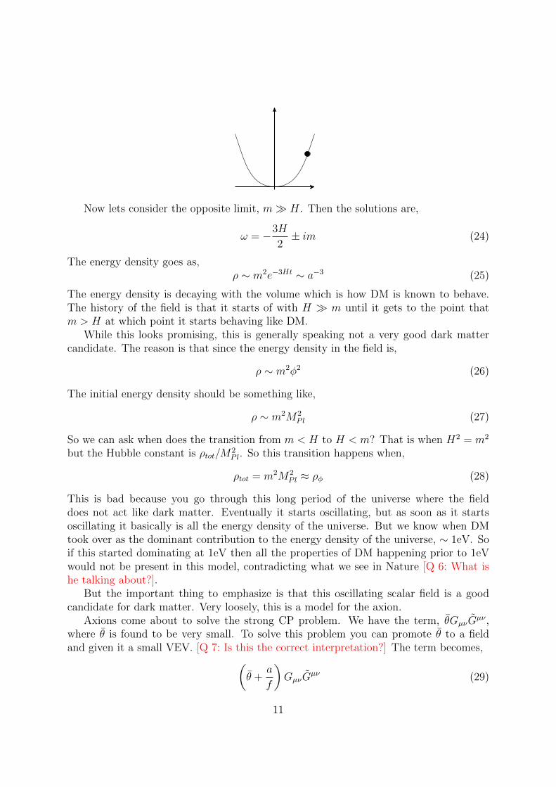
Recall that the number density for a non-relativistic particle scales like,

nχ ∼ (mτ)3/2e−m/τ (35)

So as time progresses we have,

nχnγ

timeT ≈ m

low σv

mid σv

high σv

If this system stayed in equlibrium the DM would continue to annihilate until there wasno DM at all. However, this won’t happen because eventually you’ll get to a situationwhere there are not enough DM particles around to find each other to annihilate. So ifyou have a very low cross section at one point you will break off of equilibrium.

So for some value of σv we would expect to have an appropriate amount of DM leftby tuning the cross-section.

The process of the system being in equilibrium and then stopping to be in equilibriumis called freezedown. The condition for freezeout is that,

nχ 〈σv〉 = H (36)

The left hand side is the rate that any dark matter particle floating around in the universeannhilates with another DM particle. This is the condition for freeze out since if DM hasnot found another DM particle to anniihilate with in one hubble time at that point theuniverse has essentially doubled in size. At this point the universe is much more diluteand the probability of having any more annihilations is very small.

A simple observation is to note that the temperature of the freezeout is equal to themass of the DM matter,

TFO = xmχ (37)

13

where x is some order 10 number. The reason for that is due to the exponential in thescaling of the number density. [Q 10: sharpen this.]

We can solve this becuase we have,

nFO =H

σv=

T 2

MPlσv=

m2χx

2

MPlσv(38)

That’s the number density at freezeout. What you actually want to know is the numberdensity today. Recall that the temperature scales as, T ∼ a−1. So we can write,

nnow = nFO

(aFOanow

)3

= nFO

(TnowTFO

)3

(39)

So we finally have,

nnow =m2χx

2

MPl 〈σv〉T 3now

m3χx

3(40)

with,

ρnow =T 3now

MPl 〈σv〉x(41)

The energy density now is just dicated by the photon temperature, x, v, and the cross-section. The important observation is that the energy density is determined by σv (upto order 1 factors we haven’t mentinoed here).

There is a simple way to calculate the cross-section that you need. There is thetemperature of matter radiation equality. This is the tempeature where DM had thesame energy density as radiation. This occured at about 1eV. Instead of asking what isthe temperature now we can ask what is the temperature of matter radiation equality.Using the expression above we have,

ρMRE = T 4MRF = mχnFO

T 3MRE

T 3FO

(42)

ργ =mχx

2m2χ

MPlσv

T 3MRE

x3mχ3

(43)

which implies that,T 3MRE

MPlσvx= T 4

MRE (44)

This allows you to solve for this cross section,

σv =1

xMPlTMRE

(45)

This quantity is about the TeV scale. This is referred to the Weakly Interacting MassiveParticle (WIMP) miracle. Particles with weak scale cross-sections end up giving theappropriate amount of DM.

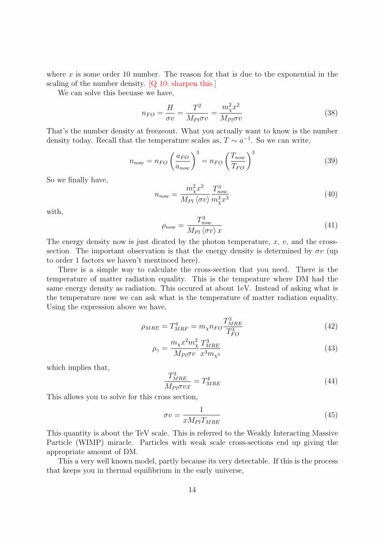
This a very well known model, partly because its very detectable. If this is the processthat keeps you in thermal equilibrium in the early universe,

14

χ

χ SM

SM

?

time (1)

time (2)

time (3)

then you’ve just measured the size of this to be, σv ∼ 1/M2W . What you’ve measured is

the size of the diagram going in the horizontal direction. One can then argue that if itexists in the horizontal direction it should also exist in the other directions. This givesus three ways to probe WIMPs. The different ways are known as follows,

(1) Indirect detection: χχ annihilation in the halo

(2) Direct detection: undergraduate experiment where you hold the DM particle willcome through and recoil onto a nucleus (this assumes the interaction involves a DMinteraction with quark or gluon).

(3) Colliders: Look for missing energy processes at the LHC.

7 Canonical WIMP

In thinking about WIMPs, its good to have in mind a canonical model. We take thismodel to be a fermion doublet under SU(2) with hypercharge ±1/2. This is recognizedas a pure Higgsino or a right handed neutrino.

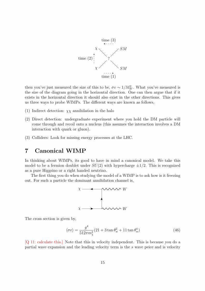
The first thing you do when studying the model of a WIMP is to ask how is it freezingout. For such a particle the dominant annihilation channel is,

χ

χ

W

W

The cross section is given by,

〈σv〉 =g4

512πm2χ

(21 + 3 tan θ2w + 11 tan θ4w) (46)

[Q 11: calculate this.] Note that this in velocity independent. This is because you do apartial wave expansion and the leading velocity term is the s wave peice and is velocity

15

independent. The target cross section is, 〈σv〉 = 3× 10−26cm3/s. You only have one freeparameter here, the dark matter particle mass. The energy density is given by,

Ωχh2 = 0.1×

( mχ

TeV

)2(47)

So we see that we need mχ ∼ TeV (about an order of magnitude above the weak scale).Now lets explore whether this is ruled out through direct detection. As a homework

exercise one can show that the differential energy rate of scattering of a dark matterparticle for a spin-independent scattering,

dR

ER= NTMN

ρχσn2mχµ2

ne

(fpz + fn(A− Z))2 F 2(ER)×∫ ∞vmin(ER)

f(v)

vdv (48)

[Q 12: What exactly is R?] The variables in this expression are,

• NT : number of targets

• MN : mass of the nucleous

• ρχ: local dark matter density (≈ 0.3GeV/cm3)

• σn: cross section per nucleon

• µne : is the reduced mass of the WIMP-nucleon system (roughly equal to mproton)

• fp and fn are the couplings to the proton and neutron

• A,Z is the atomic mass and atomic number of the nucleus

• F 2(ER) is a form factor distribution

• f(v) is the speed distribution. The usual assumption that is made is that the DMhas some Bolzmann distribution, which gives you f(v).

It has been show that, 3

σtot =G2F

2πµ2χ

((1− 4 sin2 θw)Z − (A− Z)

)2(49)

You now have to do a backwords thing. You are really interested in comparing with theexclusion plots, which show the cross-section per nucleon. This is given by,

σo =G2F

2πµχne

[...]

Λ2≈ 2× 10−39cm2 (50)

The limits are roughly given as follows:

3See a paper by Rouven Essig, 0710.1667.

16

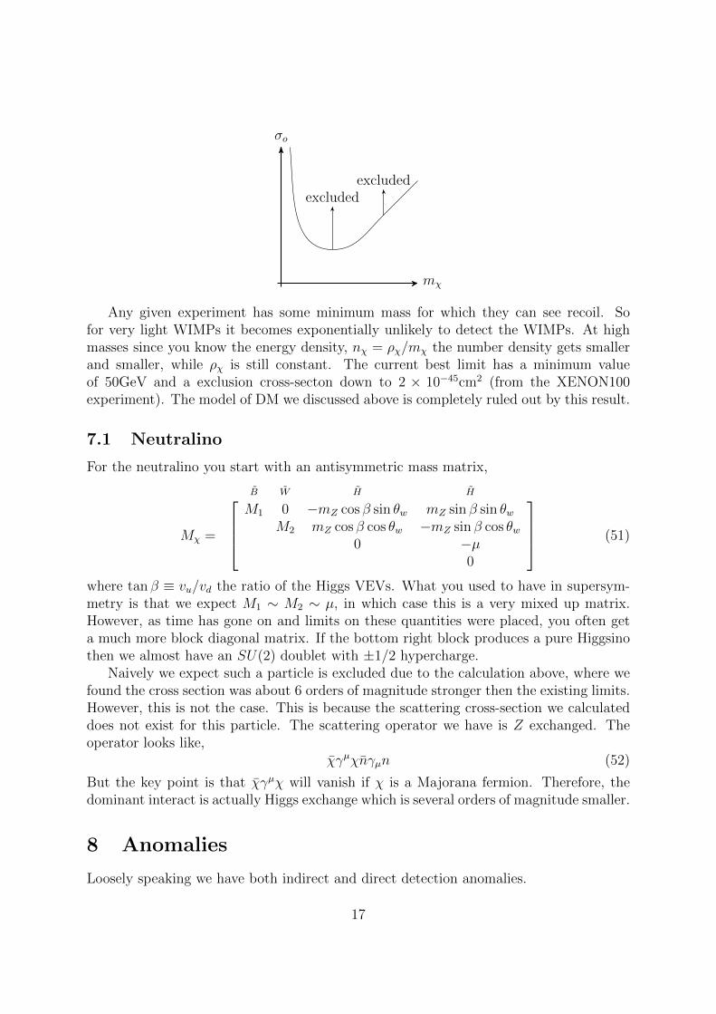
σo

mχ

excludedexcluded

Any given experiment has some minimum mass for which they can see recoil. Sofor very light WIMPs it becomes exponentially unlikely to detect the WIMPs. At highmasses since you know the energy density, nχ = ρχ/mχ the number density gets smallerand smaller, while ρχ is still constant. The current best limit has a minimum valueof 50GeV and a exclusion cross-secton down to 2 × 10−45cm2 (from the XENON100experiment). The model of DM we discussed above is completely ruled out by this result.

7.1 Neutralino

For the neutralino you start with an antisymmetric mass matrix,

Mχ =

B W H H

M1 0 −mZ cos β sin θw mZ sin β sin θwM2 mZ cos β cos θw −mZ sin β cos θw

0 −µ0

(51)

where tan β ≡ vu/vd the ratio of the Higgs VEVs. What you used to have in supersym-metry is that we expect M1 ∼ M2 ∼ µ, in which case this is a very mixed up matrix.However, as time has gone on and limits on these quantities were placed, you often geta much more block diagonal matrix. If the bottom right block produces a pure Higgsinothen we almost have an SU(2) doublet with ±1/2 hypercharge.

Naively we expect such a particle is excluded due to the calculation above, where wefound the cross section was about 6 orders of magnitude stronger then the existing limits.However, this is not the case. This is because the scattering cross-section we calculateddoes not exist for this particle. The scattering operator we have is Z exchanged. Theoperator looks like,

χγµχnγµn (52)

But the key point is that χγµχ will vanish if χ is a Majorana fermion. Therefore, thedominant interact is actually Higgs exchange which is several orders of magnitude smaller.

8 Anomalies

Loosely speaking we have both indirect and direct detection anomalies.

17

The indirect anomalies are as follows. The Fermi galactic center telescrope “bump” aswell as the Fermi 130GeV line both arise from the galactic center. There is also an excessof integral 511keV line also from the galactic center. Finally we have the Pamela/AMShigh energy positron local anomaly.

The direct anomalies are DAMA, which claims to see an annual modulation, CoGeNT,CoGeNT modulation, CRESST, CDMS-Si.

We now discuss some of these in some detail.

8.1 Indirect detection

8.1.1 Fermi line

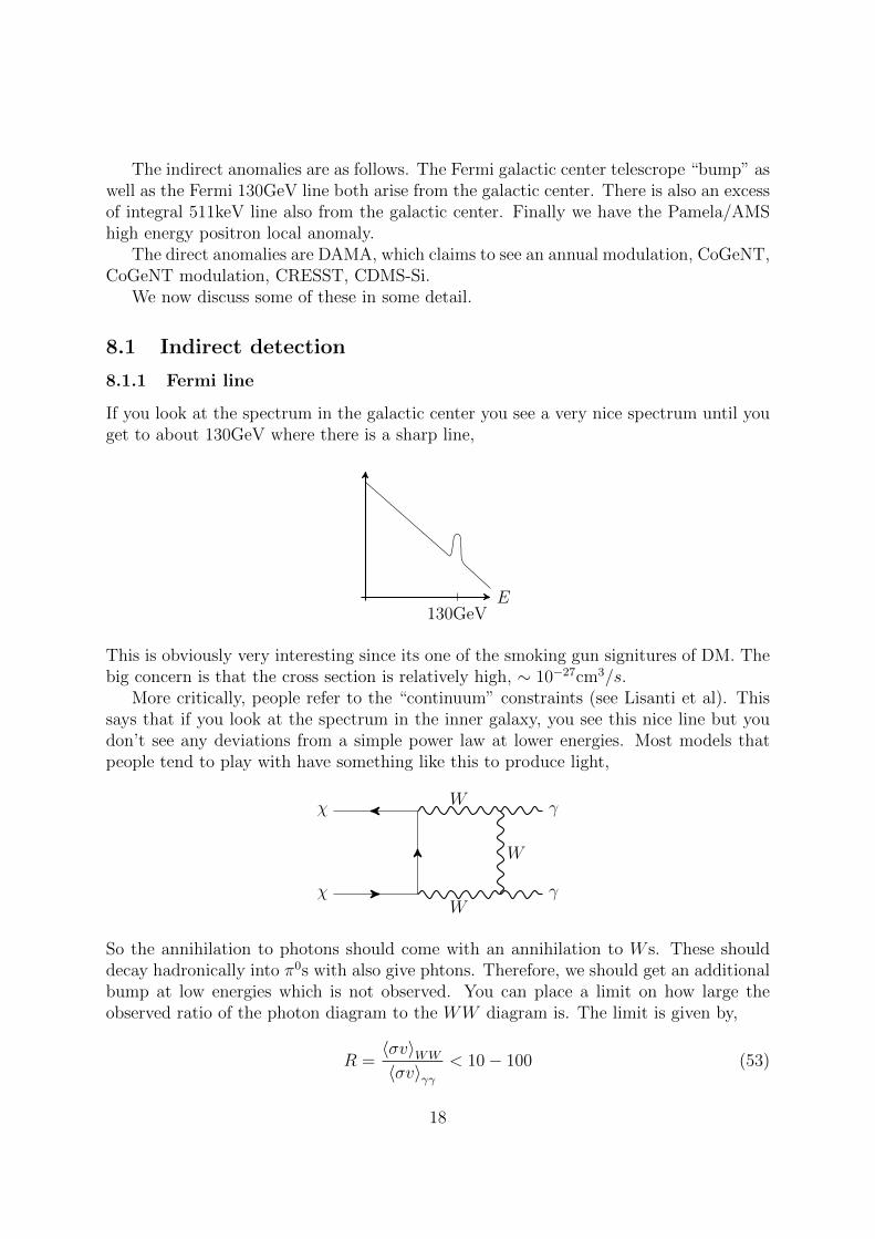
If you look at the spectrum in the galactic center you see a very nice spectrum until youget to about 130GeV where there is a sharp line,

E130GeV

This is obviously very interesting since its one of the smoking gun signitures of DM. Thebig concern is that the cross section is relatively high, ∼ 10−27cm3/s.

More critically, people refer to the “continuum” constraints (see Lisanti et al). Thissays that if you look at the spectrum in the inner galaxy, you see this nice line but youdon’t see any deviations from a simple power law at lower energies. Most models thatpeople tend to play with have something like this to produce light,

χ

χ

W

W

W

γ

γ

So the annihilation to photons should come with an annihilation to W s. These shoulddecay hadronically into π0s with also give phtons. Therefore, we should get an additionalbump at low energies which is not observed. You can place a limit on how large theobserved ratio of the photon diagram to the WW diagram is. The limit is given by,

R =〈σv〉WW

〈σv〉γγ< 10− 100 (53)

18

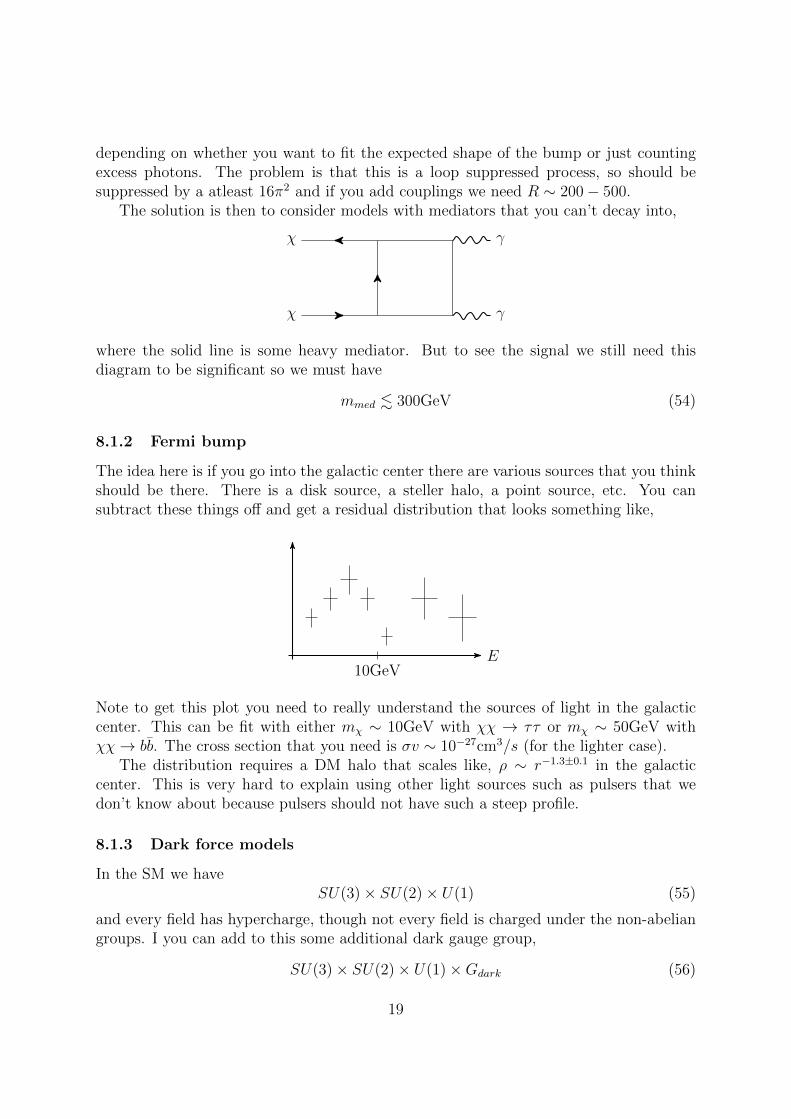
depending on whether you want to fit the expected shape of the bump or just countingexcess photons. The problem is that this is a loop suppressed process, so should besuppressed by a atleast 16π2 and if you add couplings we need R ∼ 200− 500.

The solution is then to consider models with mediators that you can’t decay into,

χ

χ

γ

γ

where the solid line is some heavy mediator. But to see the signal we still need thisdiagram to be significant so we must have

mmed . 300GeV (54)

8.1.2 Fermi bump

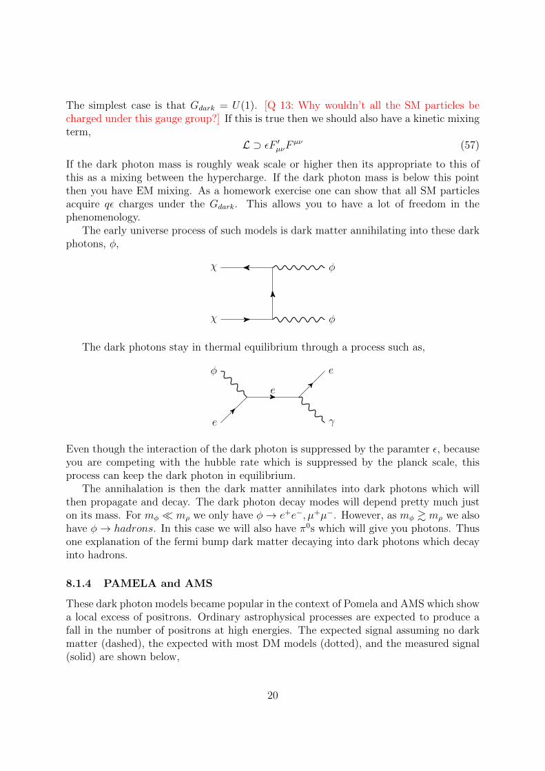
The idea here is if you go into the galactic center there are various sources that you thinkshould be there. There is a disk source, a steller halo, a point source, etc. You cansubtract these things off and get a residual distribution that looks something like,

E10GeV

Note to get this plot you need to really understand the sources of light in the galacticcenter. This can be fit with either mχ ∼ 10GeV with χχ → ττ or mχ ∼ 50GeV withχχ→ bb. The cross section that you need is σv ∼ 10−27cm3/s (for the lighter case).

The distribution requires a DM halo that scales like, ρ ∼ r−1.3±0.1 in the galacticcenter. This is very hard to explain using other light sources such as pulsers that wedon’t know about because pulsers should not have such a steep profile.

8.1.3 Dark force models

In the SM we haveSU(3)× SU(2)× U(1) (55)

and every field has hypercharge, though not every field is charged under the non-abeliangroups. I you can add to this some additional dark gauge group,

SU(3)× SU(2)× U(1)×Gdark (56)

19

The simplest case is that Gdark = U(1). [Q 13: Why wouldn’t all the SM particles becharged under this gauge group?] If this is true then we should also have a kinetic mixingterm,

L ⊃ εF ′µνFµν (57)

If the dark photon mass is roughly weak scale or higher then its appropriate to this ofthis as a mixing between the hypercharge. If the dark photon mass is below this pointthen you have EM mixing. As a homework exercise one can show that all SM particlesacquire qε charges under the Gdark. This allows you to have a lot of freedom in thephenomenology.

The early universe process of such models is dark matter annihilating into these darkphotons, φ,

χ

χ

φ

φ

The dark photons stay in thermal equilibrium through a process such as,

e

φ

e

e

γ

Even though the interaction of the dark photon is suppressed by the paramter ε, becauseyou are competing with the hubble rate which is suppressed by the planck scale, thisprocess can keep the dark photon in equilibrium.

The annihalation is then the dark matter annihilates into dark photons which willthen propagate and decay. The dark photon decay modes will depend pretty much juston its mass. For mφ mρ we only have φ→ e+e−, µ+µ−. However, as mφ & mρ we alsohave φ→ hadrons. In this case we will also have π0s which will give you photons. Thusone explanation of the fermi bump dark matter decaying into dark photons which decayinto hadrons.

8.1.4 PAMELA and AMS

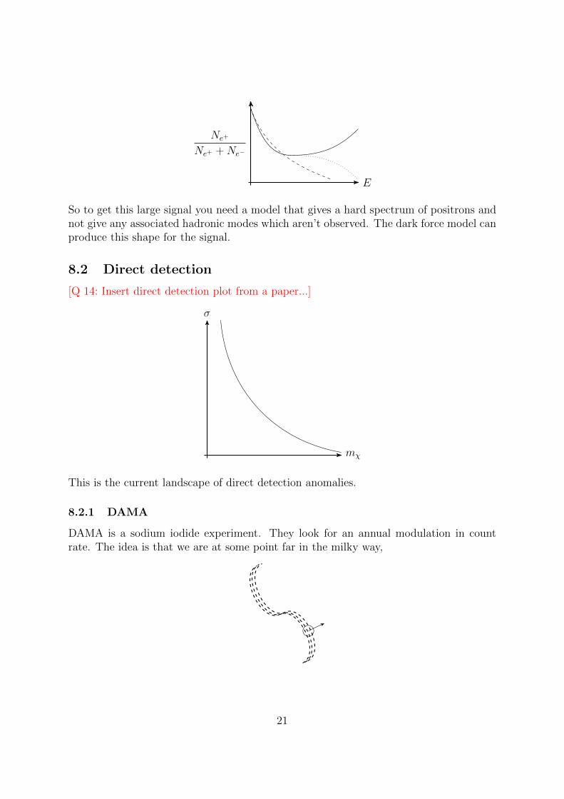
These dark photon models became popular in the context of Pomela and AMS which showa local excess of positrons. Ordinary astrophysical processes are expected to produce afall in the number of positrons at high energies. The expected signal assuming no darkmatter (dashed), the expected with most DM models (dotted), and the measured signal(solid) are shown below,

20

Ne+

Ne+ +Ne−

E

So to get this large signal you need a model that gives a hard spectrum of positrons andnot give any associated hadronic modes which aren’t observed. The dark force model canproduce this shape for the signal.

8.2 Direct detection

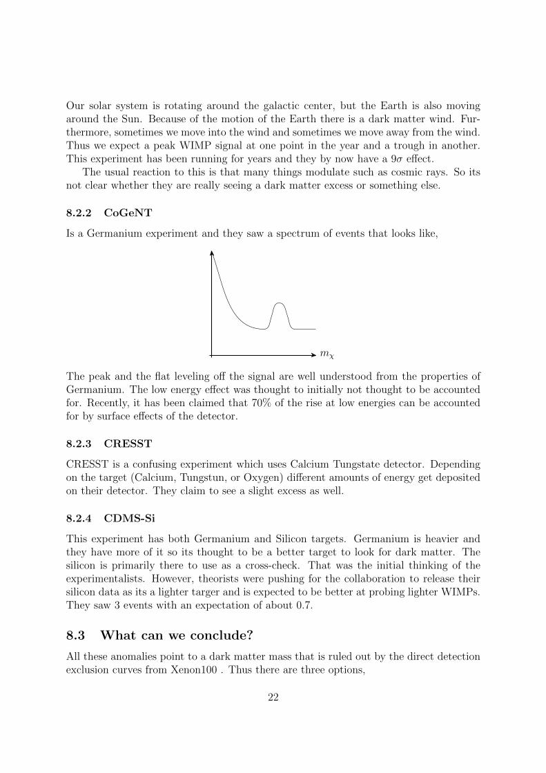
[Q 14: Insert direct detection plot from a paper...]

σ

mχ

This is the current landscape of direct detection anomalies.

8.2.1 DAMA

DAMA is a sodium iodide experiment. They look for an annual modulation in countrate. The idea is that we are at some point far in the milky way,

21

Our solar system is rotating around the galactic center, but the Earth is also movingaround the Sun. Because of the motion of the Earth there is a dark matter wind. Fur-thermore, sometimes we move into the wind and sometimes we move away from the wind.Thus we expect a peak WIMP signal at one point in the year and a trough in another.This experiment has been running for years and they by now have a 9σ effect.

The usual reaction to this is that many things modulate such as cosmic rays. So itsnot clear whether they are really seeing a dark matter excess or something else.

8.2.2 CoGeNT

Is a Germanium experiment and they saw a spectrum of events that looks like,

mχ

The peak and the flat leveling off the signal are well understood from the properties ofGermanium. The low energy effect was thought to initially not thought to be accountedfor. Recently, it has been claimed that 70% of the rise at low energies can be accountedfor by surface effects of the detector.

8.2.3 CRESST

CRESST is a confusing experiment which uses Calcium Tungstate detector. Dependingon the target (Calcium, Tungstun, or Oxygen) different amounts of energy get depositedon their detector. They claim to see a slight excess as well.

8.2.4 CDMS-Si

This experiment has both Germanium and Silicon targets. Germanium is heavier andthey have more of it so its thought to be a better target to look for dark matter. Thesilicon is primarily there to use as a cross-check. That was the initial thinking of theexperimentalists. However, theorists were pushing for the collaboration to release theirsilicon data as its a lighter targer and is expected to be better at probing lighter WIMPs.They saw 3 events with an expectation of about 0.7.

8.3 What can we conclude?

All these anomalies point to a dark matter mass that is ruled out by the direct detectionexclusion curves from Xenon100 . Thus there are three options,

22

1. Experiments are wrong

2. Astrophysics is wrong

3. Model is wrong

There are a few ways to bypass the exclusion curves but still produce anomalies,

• Inelastic endothermic scattering

– Favors heavy targets

• Inelastic exothermic scattering

– Favors light targets

• Momentum dependent interactions

– Favors experiments with high thresholds

• Spin dependent interactions

– Favors targets with spin

• Isospin dependent interactions (fp 6= fn)

– Kill 1 experiment

• Electron scattering

– Favors non-descriminitory experiments

These tricks will favor one experiment over another one and shift the curves above whichassume you can compare all the experiments. .

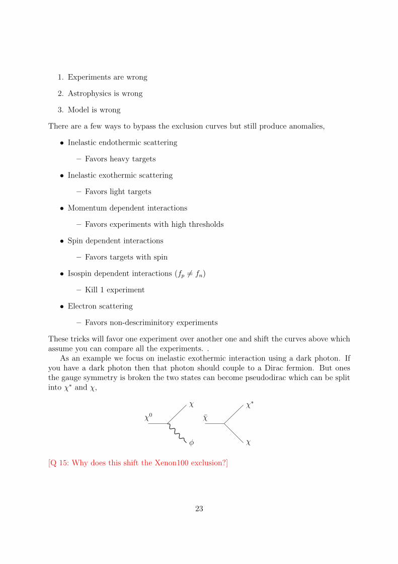
As an example we focus on inelastic exothermic interaction using a dark photon. Ifyou have a dark photon then that photon should couple to a Dirac fermion. But onesthe gauge symmetry is broken the two states can become pseudodirac which can be splitinto χ∗ and χ,

χ0

χ

φ

χ

χ

χ∗

[Q 15: Why does this shift the Xenon100 exclusion?]

23