Dark Energy at the Crossroads

Dragan Huterer Physics Department, University of Michigan

Key contributions from grad students: Jessie Muir, Noah Weaverdyck (current)

Daniel Shafer, Eduardo Ruiz (former)

4%

22%

74%

Makeup of universe today

Dark Matter(suspected since 1930sestablished since 1970s)

Dark Energy(suspected since 1980sestablished since 1998)

Also: radiation (0.01%)

Baryonic Matter(stars 0.4%, gas 3.6%)

Evidence for Dark energy from type Ia Supernovae

Union2 SN compilation binned in redshift

⌦DE ⌘ �DE

�crit

w ⌘ pDE

�DE

Current evidence for dark energy is impressively strong

Dan Shafer

SN + BAO + CMB: ΩΛ=0.724±0.010 ΩΛ=0 is 72-σ away

Fine Tuning Problem: “Why so small”?

Vacuum Energy: Quantum Field Theory predicts it to be determined by cutoff scale

60-120 orders of magnitude smaller than expected!

Planck scale:

SUSY scale: (1019 GeV)4(1 TeV)4 }(10−3eV)4Measured:

⇥VAC =12

�

fields

gi

⇥ �

0

⇤k2 + m2

d3k

(2�)3�

�

fields

gik4max

16�2

V

φ

Lots of theoretical ideas, few compelling ones:Very difficult to motivate DE naturally

E.g. ‘quintessence’ (evolving scalar field)

mφ ≃ H0 ≃ 10−33 eV

�̈+ 3H�̇+dV

d�= 0

Ratra & Peebles, 1988 Zlatev, Wang & Steinhardt, 1999

String landscape? ⇒ A time of desperation?

0 10−120 MPL4 MPL

4 ρΛ

Among the ∼10500 minima, we live in one that allows structure/galaxies to form(selection effect) (anthropic principle)

Pam Jeffries

Kolb & Turner, “Early Universe”, footnote on p. 269: “It is not clear to one of the authors how a concept as lame

as the “anthropic idea” was ever elevated to the status of a principle”

Landscape “predicts” the observed ΩDE

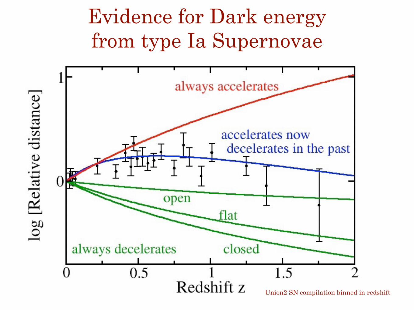
A difficulty: DE theory target accuracy, in e.g. w(z),

not known a priori

(Δm2)sol ≃ 8×10−5 eV2

(Δm2)atm ≃ 3×10−3 eV2

Contrast this situation with:

1. Neutrino masses:∑mi = 0.06 eV* (normal)}∑mi = 0.11 eV* (inverted)

*(assuming m3=0)

vs.

2. Higgs Boson mass (before LHC 2012):mH ≲ O(200) GeV

(assuming Standard Model Higgs)

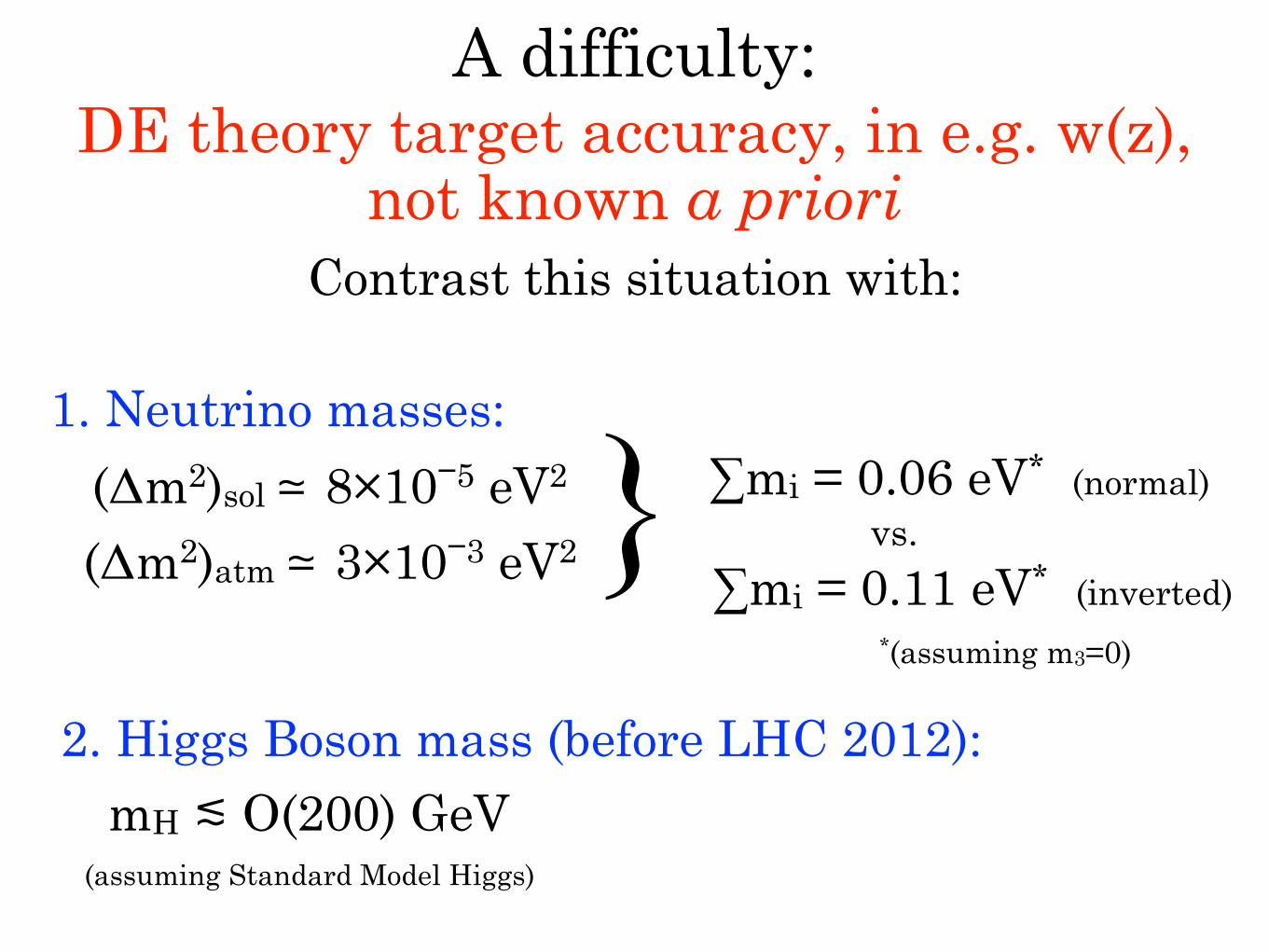
Planck Collaboration: Planck 2015 results. XIV. Dark energy and modified gravity

0.0 0.5 1.0 1.5 2.0

z

�1.5

�1.0

�0.5

0.0

w(z

)

Planck+BSH

Fig. 7. PCA analysis constraints (described in Sect. 5.1.3). Thetop panel shows the reconstructed equation of state w(z) after thePCA analysis. Vertical error bars correspond to mean and stan-dard deviations of the q vector parameters, while horizontal errorbars are the amplitude of the original binning. The bottom panelshows the PCA corresponding weights on w(z) as a function ofredshift for the combination Planck TT+lowP+BSH.

equal. The function F(x) in Eq. (23) is defined as:

F(x) ⌘p

1 + x3

x3/2 �ln⇣x3/2 +

p1 + x3

⌘

x3 . (25)

Eq. (23) parameterizes w(a) with one parameter ✏s, while adedepends on ⌦m and ✏s and can be derived using an approxi-mated fitting formula that facilitates numerical computation(Huang et al. 2011). Positive (negative) values of ✏s correspondto quintessence (phantom) models.

Eq. (23) is only valid for late-Universe slow-roll (✏V . 1and ⌘V ⌘ M2

PV 00/V ⌧ 1) or the moderate-roll (✏V . 1 and⌘V . 1) regime. For quintessence models, where the scalar fieldrolls down from a very steep potential, at early times ✏V(a) � 1,however the fractional density ⌦�(a) ! 0 and the combination✏V(a)⌦�(a) aprroaches a constant, defined to be a second param-eter ✏1 ⌘ lima!0 ✏V(a)⌦�(a).

One could also add a third parameter ⇣s to capture the time-dependence of ✏V via corrections to the functional dependenceof w(a) at late time. This parameter is defined as the relativedi↵erence of d

p✏V⌦�/dy at a = ade and at a ! 0, where y ⌘

(a/ade)3/2/p

1 + (a/ade)3. If ✏1 ⌧ 1, ⇣s is proportional to thesecond derivative of ln V(�), but for large ✏1, the dependence ismore complicated (Huang et al. 2011). In other words, while ✏sis sensitive to the late time evolution of 1 + w(a), ✏1 capturesits early time behaviour. Quintessence/phantom models can bemapped into ✏s–✏1 space and the classification can be furtherrefined with ⇣s. For ⇤CDM, all three parameters are zero.

In Fig. 8 we show the marginalized posterior distribu-tions at 68.3 % and 95.4 % confidence levels in the param-eter space ✏s–⌦m, marginalizing over the other parameters.In Fig. 9 we show the current constraints on quintessencemodels projected in ✏s–✏1 space. The constraints are ob-tained by marginalizing over all other cosmological parameters.The models here include exponentials V = V0 exp(���/MP)(Wetterich 1988), cosines from pseudo-Nambu Goldstonebosons (pnGB) V = V0[1 + cos(��/MP)] (Frieman et al.1995; Kaloper & Sorbo 2006), power laws V = V0(�/MP)�n

(Ratra & Peebles 1988), and models motivated by supergrav-ity (SUGRA) V = V0(�/MP)�↵ exp [(�/MP)2] (Brax & Martin1999). The model projection is done with a fiducial ⌦m = 0.3cosmology. We have verified that variations of 1 % compared tothe fiducial ⌦m lead to negligible changes in the constraints.

Mean values and uncertainties for a selection of cosmo-logical parameters are shown in Table 2, for both the 1-parameter case (i.e., ✏s only, with ✏1 = 0 and ⇣s = 0, de-scribing “thawing” quintessence/phantom models, where �̇ =0 in the early Universe) and the 3-parameter case (generalquintessence/phantom models where an early-Universe fast-rolling phase is allowed). When we vary the data sets and the-oretical prior (between the 1-parameter and 3-parameter cases),the results are all compatible with ⇤CDM and mutually compat-ible with each other. Because ✏s and ✏1 are correlated, cautionhas to be taken when looking at the marginalized constraintsin the table. For instance, the constraint on ✏s is tighter for the3-parameter case, because in this case flatter potentials are pre-ferred in the late Universe in order to slow-down larger �̇ fromthe early Universe. A better view of the mutual consistency canbe obtained from Fig. 9. We find that the addition of polariza-tion data does not have a large impact on these DE parameters.Adding polarization data to Planck+BSH shifts the mean of ✏sby �1/6� and reduces the uncertainty of ✏s by 20 %, while the95 % upper bound on ✏1 remains unchanged.

5.1.5. Dark energy density at early times

Quintessence models can be divided into two classes, namelycosmologies with or without DE at early times. Although theequation of state and the DE density are related to each other,it is often convenient to think directly in terms of DE densityrather than the equation of state. In this section we provide amore direct estimate of how much DE is allowed by the dataas a function of time. A key parameter for this purpose is ⌦e,which measures the amount of DE present at early times (“earlydark energy,” EDE) (Wetterich 2004). Early DE parameteriza-tions encompass features of a large class of dynamical DE mo-dels. The amount of early DE influences CMB peaks and can bestrongly constrained when including small-scale measurementsand CMB lensing. Assuming a constant fraction of ⌦e until re-cent times (Doran & Robbers 2006), the DE density is parame-terized as:

⌦de(a) =⌦0

de �⌦e(1 � a�3w0 )⌦0

de +⌦0ma3w0

+⌦e(1 � a�3w0 ) . (26)

13

Planck XIV, “Dark Energy and Modified Gravity”, arXiv:1502.01590

Current constraints on w(z): largely from geometrical measures

BAO+ SNIa+

Hubble const

Dark Energy suppresses the growth of density fluctuations

The Virgo Consortium (1996)

with DE

without DE

Today1/4 size of today 1/2 size of today(a=1/4 or z=3) (a=1/2 or z=1) (a=1 or z=0)

Huterer et al, Snowmass report, 1309.5385

Next Frontier: Growth (+geom) from LSS

CMB LSS

dimension 2D 3D

# modes ∝lmax2 ∝kmax

3

can slice in λ only λ, M, bias...

temporal evol. no yes

systematics? relatively clean relatively messy

theory modeling easy can be hard

Using growth to separate GR from MG:

H2− F (H) =

8πG

3ρ, or H2 =

8πG

3

!

ρ +3F (H)

8πG

"

For example:

Modified gravity GR + dark energy

Growth of density fluctuations can decide:

�̈ + 2H �̇ � 4⇡G⇢M� = 0(assuming GR)

Remainder of talk: three sets of dark energy tests

with LSS

1. Separating growth from geometry using current data

2. Measuring covariance of peculiar velocities of nearby SN/gals to test LCDM

3. Blinding the DES analysis.

1. Separating geometry and growth2

program has been started very successfully byWang et al.[17] (see also [18–20] which contained very similar ideas),who used data available at the time; the constraints how-ever were weak. Our overall philosophy and approachare similar as those in Refs. [17–20], but we benefit enor-mously from the new data and increased sophisticationin understanding and modeling them, as well as the avail-ability of a few additional cosmological probes not avail-able in 2007.

The paper is divided as follows: we present the reason-ing behind our approach in section II. In section III wereview the cosmological probes used in the analysis. Areview of the analysis method is provided in section IV,and we present our constraints on parameters in sectionV. We discuss these results in section VI, and give finalremarks in section VII.

II. PHILOSOPHY OF OUR APPROACH

We would like to perform stringent but general consis-tency tests of the currently favored ⇤CDM cosmologicalmodel with ⇠25% dark plus baryonic matter and ⇠75%dark energy, as well as the more general wCDM model.The ⇤CDM model, favored since even before the directdiscovery of the accelerating universe (e.g. [21]), is in ex-cellent agreement with essentially all cosmological data,despite occasional mild warnings to the contrary ([22–25]). There has been a huge amount of e↵ort devotedto tests alternative to wCDM – most notably, modifiedgravity models where modifications to Einstein’s Gen-eral Theory of Relativity, imposed to become importantat late times in the evolution of the universe and at largespatial scales, make it appear as if the universe is accel-erating if interpreted assuming standard GR.

Here we take a complementary approach, and studythe internal consistency of the wCDM model itself, with-out assuming any alternative model. We split the cosmo-logical information describing the late universe into twoclasses:

• Geometry: expansion rate H(z) and the comovingdistance r(z), and associated derived quantities.

• Growth: growth rate of density fluctuations in lin-ear (D(z) ⌘ �(z)/�(0)) and non-linear regime.

Regardless of the parametric description of the geome-try and growth sectors, one thing is clear: in the standardmodel that assumes General Relativity with its usual re-lations between the growth and distances, the split pa-rameters Xgeom

i and Xgrowi have to agree – that is, be

consistent with each other at some statistically appro-priate confidence level. Any disagreement between theparameters in the two sectors, barring unforseen remain-ing systematic errors, can be interpreted as the violationof the standard cosmological model assumption.

The split parameter constraints provide very general,yet powerful, tests of the dominant paradigm. They can

Cosmological Probe Geometry Growth

SN Ia H0

DL(z) —–

BAO

✓D2

A(z)H(z)

◆1/3

/rs(zd) —–

CMB peak loc. R /p

⌦mH2

0

DA(z⇤) —–

Cluster countsdV

dz

dn

dM

Weak lens 2ptr2(z)H(z)

Wi(z)Wj(z) P

✓k =

`

r(z)

◆

RSD F (z) / DA(z)H(z) f(z)�8

(z)

TABLE I. Summary of cosmological probes that we used andaspects of geometry and growth that they are sensitive to.The assignments in the second and third column are neces-sarily approximate given the short space in the table; moredetail is given in respective sections covering our use of thesecosmological probes. Here rs(zd) refers to the sound horizonevaluated at the baryon drag epoch zd.

be compared to more specific parametrizations of depar-tures from GR — for example, the � parametrization[26], or the various schemes of the aforementioned com-parison of the Newtonian potentials. Our approach iscomplementary to these more specific parametrizations:while perhaps not as powerful in specific instances, it isequipped with more freedom to capture departures fromthe standard model.Most of the cosmological measurements involve large

amounts of raw data, and their information is often com-pressed into a very small number of meta-parameters.For example, weak lensing shows the two-point cor-relation function, cluster number counts are given inmass bins, while baryon acoustic oscillations, cosmicmicrowave background, and redshift space distortionsinformation is often captured in a small number ofmeta-parameters which are defined and presented below.[Type Ia supernovae are somewhat of an exception, sincewe use individual magnitude measurements from eachSN from the beginning.] Given that in some cases oneassumes the cosmological model (often ⇤CDM) to derivethese intermediate parameters, the question is whetherwe should worry about using the meta-parameters toconstrain the wider class of cosmological models wheregrowth history is decoupled from geometry. Fortunately,in this particular case our constraints are robust: cer-tainly for surveys that specialize in either geometry andgrowth alone, the meta-parameters are de facto correctby construction, and capture nearly all cosmological in-formation of interest. For probes that are sensitive toboth growth and geometry, like the weak lensing andcluster counts, the quantities used for the analysis —correlation functions and number counts, respectively —provide a general enough representation of the raw datathat one can relax the assumption that growth and ge-ometry are consistent without the loss of robustness and

Ruiz & Huterer 2015

Idea: compare geometry and growthsee also: Wang, Hui, May & Haiman 2007

Ruiz & Huterer 2015

Our approach:

Double the standard DE parameter space (ΩM=1−ΩDE and w):

⇒ ΩMgeom

, wgeom ΩMgrow

, wgrow

[In addition to other:standard parameters: ΩMh2 ΩBh2, ns, A)nuisance parameters: probe-dependent]

(Current) Data used

SNIa

Clusters (MaxBCG)

BAO (6dF, SDSS LRG, BOSS CMASS)

Weak Lensing (CFHTLens)

CMB (Planck peak location)

RSD

r⟂

r‖

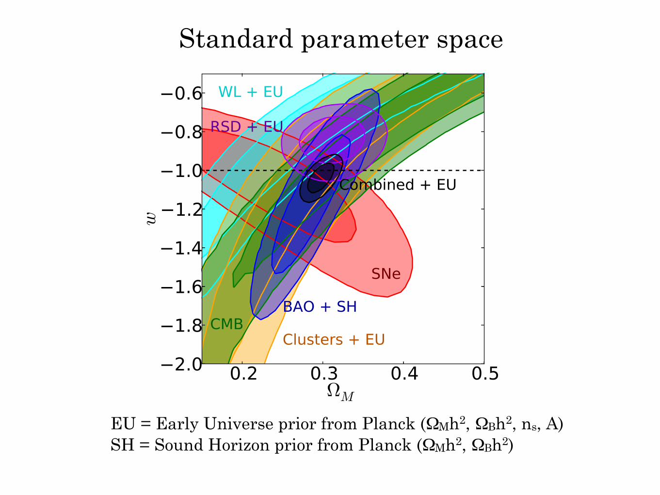
Standard parameter space

EU = Early Universe prior from Planck (ΩMh2, ΩBh2, ns, A) SH = Sound Horizon prior from Planck (ΩMh2, ΩBh2)

w (eq of state of DE): geometry vs. growth

Evidence for wgrow > wgeom:

3.3-σ

Ruiz & Huterer 2015

* SN not the recalibrated JLA

compilation - need to update; will move wgeom up

Redshift Space Distortion data

RSD prefer wgrow > −1 (slower growth than in LCDM)

(evidence 3.1-σ) (evidence 2.3-σ)

Therefore: growth probes point to even less growth

than LCDM with ~Planck parameters (i.e. wgrow > −1)

Probably equivalent to these recent findings: ● σ8 from clusters is lower than that from CMB (eg. Chon & Bohringer, Hou et al, Bocquet et al, Costanzi et al) ● σ8 from lensing is lower than that from CMB (eg. MacCrann et al) ● evidence for neutrino mass (eg. Beutler et al, Dvorkin et al) ● evidence for interactions in the dark energy sector (eg. Salvatelli et al)

(but the evidence is still not very strong...)

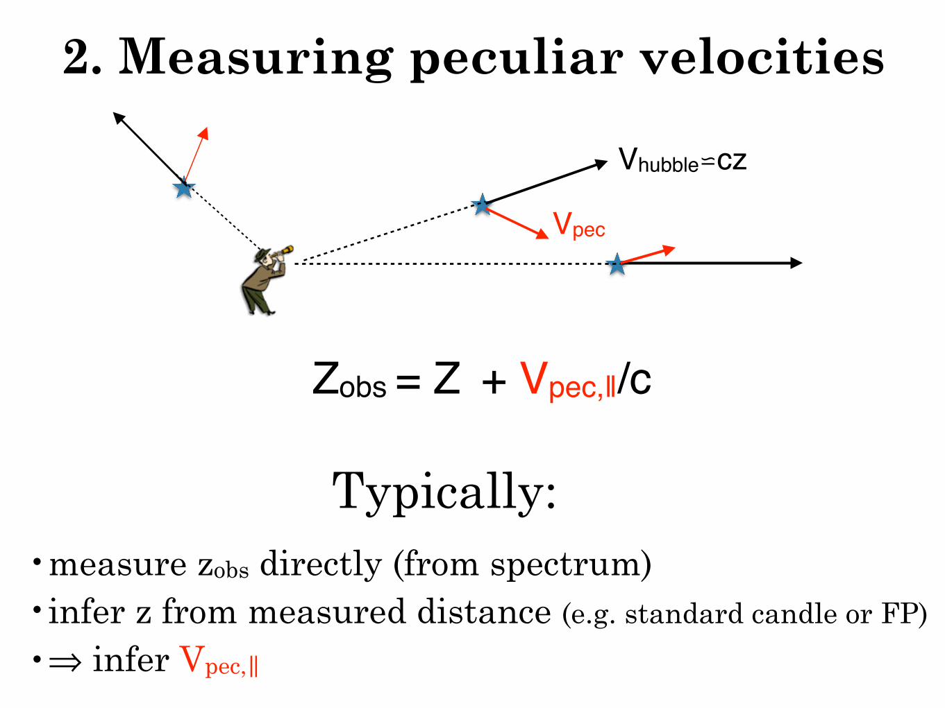
Vhubble⋍cz

Vpec

Zobs = Z + Vpec,‖/c

2. Measuring peculiar velocities

Typically:•measure zobs directly (from spectrum) •infer z from measured distance (e.g. standard candle or FP) •⇒ infer Vpec,‖

100× zCMB

1.1 1.4 1.7 2.2 2.5 3.0 3.5 4.4

100×

zCMB

1.1

1.4

1.7

2.2

2.5

3.0

3.5

4.4

-0.02

-0.01

0

0.01

0.02

0.03

0.04

0.05

100× zCMB

1.1 1.4 1.7 2.2 2.5 3.0 3.5 4.4

100×

zCMB

1.1

1.4

1.7

2.2

2.5

3.0

3.5

4.4

-0.02

-0.01

0

0.01

0.02

0.03

0.04

0.05

Signal Noise

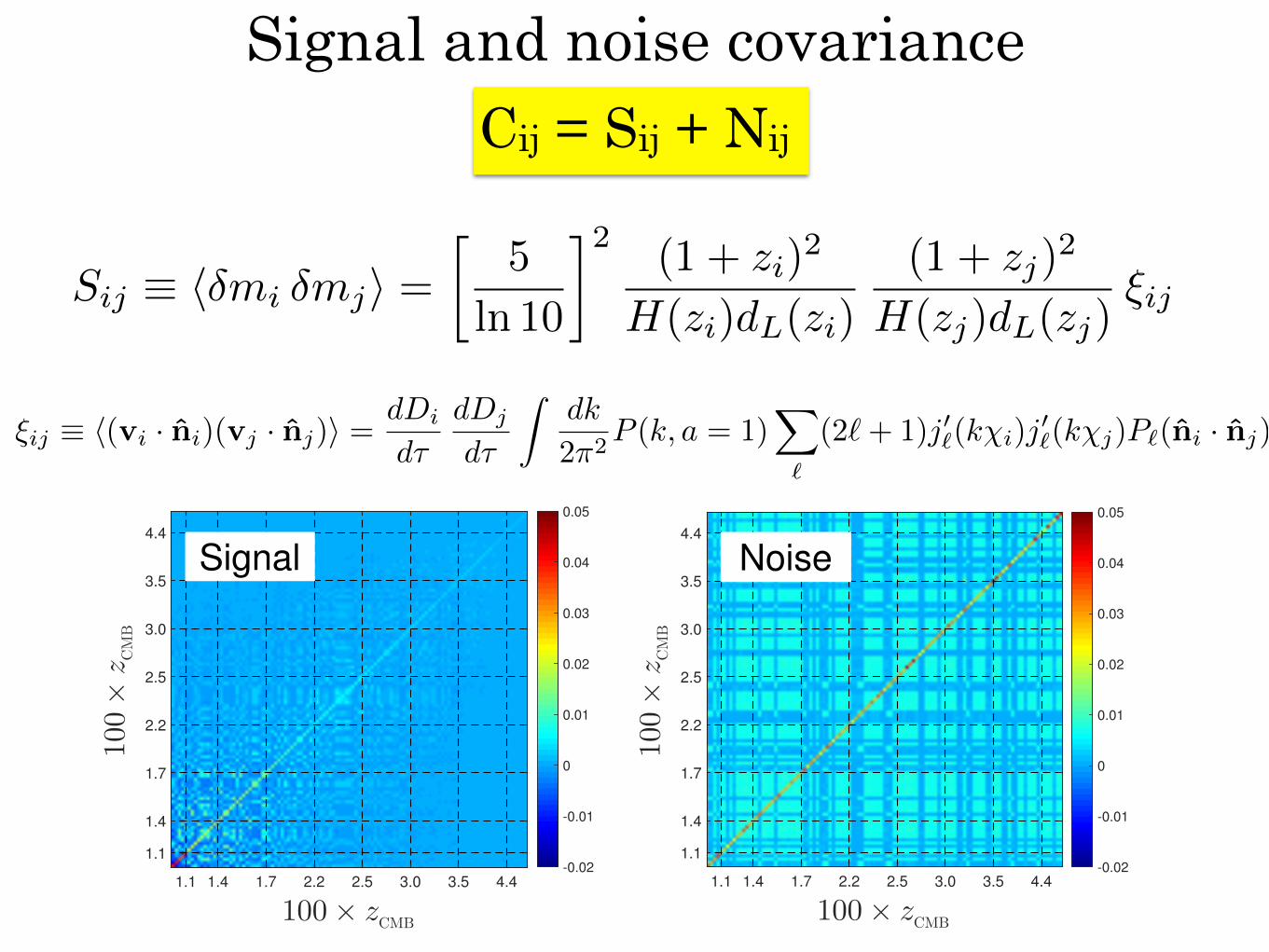
Figure 1. Comparison of the signal (left panel) and noise (right panel) contributions to the fullcovariance matrix for the 111 SNe at z < 0.05 from the JLA compilation.

Putting these ingredients together, we construct a multivariate Gaussian likelihood6

L(A,vbulk

) / 1p|C|

exp

�1

2�m

|C

�1

�m

�, (4.3)

where the elements of the vector �m are

(�m)i

= mcorr

i

�mth(zi

,M,⌦m

)��mbulk

i

(vbulk

) , (4.4)

where mcorr

i

are the observed, corrected magnitudes and mth(zi

,M,⌦m

) are the theoreticalpredictions for the background cosmological model (see below). The M parameter corre-sponds to the (unknown) absolute calibration of SNe Ia; we analytically marginalize over itin all analyses (e.g. appendix of [20]).

We emphasize that, since the covariance depends on the parameter A that we areinterested in constraining, we need to include a term for the 1/

p|C| prefactor in addition to

the usual �2 quantity. Since the covariance is a strictly increasing function of A, neglectingthe prefactor would lead to the clearly erroneous result that the likelihood is a maximum forA ! 1.

The likelihood in eq. (4.3) is the principal tool we will use for our analyses. In thismost general form, the likelihood depends on two input quantities (four parameters, sincethe velocity has three components): the normalization A of the signal component of thecovariance matrix and the excess bulk velocity v

bulk

not captured by the velocity covariance.Note that, in the fiducial model, A = 1 and v

bulk

= 0.Throughout our analyses, we assume a flat ⇤CDM model (w = �1, ⌦

k

= 0) with freeparameters fixed to values consistent with data from Planck [21] and other probes. That is, wefix ⌦

m

= 0.3, physical matter density ⌦m

h2 = 0.14, physical baryon density ⌦b

h2 = 0.0223,

6Note that SN flux, or a quantity linearly related to it, might be a better choice for the observable thanthe magnitude, given that we expect the error distribution of the former to be more Gaussian than the latter.Nevertheless, this choice should not impact our results, as the fractional errors in flux are not too large, andwe have explicitly checked that the distribution of the observed magnitudes around the mean is approximatelyGaussian. Therefore we follow most literature on the subject and work directly with magnitudes.

– 8 –

Signal and noise covarianceCij = Sij + Nij

Sij ⌘ h�mi �mji =

5

ln 10

�2 (1 + zi)2

H(zi)dL(zi)

(1 + zj)2

H(zj)dL(zj)⇠ij

⇠ij ⌘ h(vi · n̂i)(vj · n̂j)i =dDi

d⌧

dDj

d⌧

Zdk

2⇡2P (k, a = 1)

X

`

(2`+ 1)j0`(k�i)j0`(k�j)P`(n̂i · n̂j)

Using vpec to test cosmology

This is a mature subject

Our contribution:

•Significantly streamlined and simplified analysis/likelihood approach

•Using best SN sample to date (Supercal; 208 objects at z<0.1): all objects fitted and calibrated using the same technology (Scolnic et al 2015)

•Analysis is robust: we marginalize over systematic parameters, check alternate assumptions in fits. [Note: systematics still a concern.]

Huterer, Shafer, Scolnic & Schmidt, on arXiv soonHuterer, Shafer & Schmidt, JCAP, 2016

Kaiser 1989, Gorski et al 1989, Willick & Strauss 1995, Hui & Greene 2005, Watkins et al 2012,…

0 50 100 150 200 250 300 350

l (deg)

-80

-60

-40

-20

0

20

40

60

80

b(deg)

Supercal SNe and 6dF galaxies

Do the SN and galaxy data prefer signal covariance?

0 0.5 1 1.5 2 2.5

A

0

0.5

1

1.5

2

Lik

elih

ood

SN Ia (Supercal)

Galaxy FP (6dF)

Combined

Cij = ASij + Nij

11-σ detection of covariances; A=1.05+0.25−0.21

Huterer, Shafer, Scolnic & Schmidt, on arXiv soon

A=1: LCDM

A=0: pure noise

0 0.2 0.4 0.6 0.8z

0

0.1

0.2

0.3

0.4

0.5

0.6

f(z)σ

8(z)

6dF+6dF

GAMA

Wigglez BOSSVIPERSThis work

SN

Equivalently, we have a 11% meas. of fσ8

f (z)σ 8(z) = d lnDd lna

[σ 8D(z)]

fσ 8 = 0.428−0.045+0.048 @ z⋍0.02

•Ground photometric: ‣Dark Energy Survey (DES)

‣Pan-STARRS

‣Hyper Suprime Cam (HSC)

‣Large Synoptic Survey Telescope (LSST)

•Ground spectroscopic: ‣Hobby Eberly Telescope DE Experiment (HETDEX)

‣Prime Focus Spectrograph (PFS)

‣Dark Energy Spectroscopic Instrument (DESI)

•Space: ‣Euclid

‣Wide Field InfraRed Space Telescope (WFIRST)

Ongoing or upcoming DE experiments:

Dark Energy Survey (DES) Imaging survey over 5000 sq deg

Dark Energy Spectroscopic Instr. (DESI) Spectroscopic survey over 15,000 sq deg

Blanco telescope at Cerro Tololo, Chile

Mayall telescope at Kitt Peak, Arizona

ferrule holder (on eccentric arm)eccentric axis (Φ) bearing

retaining threads

Θ motor

+ +

Θ

Φ

106 μmfiber

central axisΘ bearing

controlelectronics

Φ motor

Fiber positioner @UM (×5000)

Story so far:Dark energy measurements definitely in the precision regime - impressive constraints… …but the really big questions (nature of DE) unanswered Potential to improve constraints from upcoming surveys

Planck Collaboration: Cosmological parameters

0

20

40

60

80

100

CE

E�

[10�

5µK

2]

30 500 1000 1500 2000

�

-404

�C

EE

�

Fig. 3. Frequency-averaged T E and EE spectra (without fitting for temperature-to-polarization leakage). The theoretical T E andEE spectra plotted in the upper panel of each plot are computed from the Planck TT+lowP best-fit model of Fig. 1. Residuals withrespect to this theoretical model are shown in the lower panel in each plot. The error bars show ±1� errors. The green lines in thelower panels show the best-fit temperature-to-polarization leakage model of Eqs. (11a) and (11b), fitted separately to the T E andEE spectra.

13

Planck Collaboration: Cosmological parameters

-140

-70

0

70

140

DT

E`

[µK

2]

30 500 1000 1500 2000

`

-100

10

�D

TE

`

Fig. 3. Frequency-averaged T E and EE spectra (without fitting for temperature-to-polarization leakage). The theoretical T E andEE spectra plotted in the upper panel of each plot are computed from the Planck TT+lowP best-fit model of Fig. 1. Residuals withrespect to this theoretical model are shown in the lower panel in each plot. The error bars show ±1� errors. The green lines in thelower panels show the best-fit temperature-to-polarization leakage model of Eqs. (11a) and (11b), fitted separately to the T E andEE spectra.

13

temp-temp temp-pol pol-polBut are Planck++ constraints so good that they bias us?

Danger of declaring currently favored model to be the truth blinding new data is key⇒

3. Blinding the DES analysis

Our requirements: • Preserve inter-consistency of cosmological probes • Preserve ability to test for systematic errors

Muir, Elsner, Bernstein, Huterer, Peiris and DES collab.

Our choice is specifically:

ξijblinded (k) = ξij

measured (k) ξij

model 1(k)ξij

model 2 (k)⎡

⎣⎢

⎤

⎦⎥

Tests passed, black-box code ready. First application expected for clustering measurements in DES year-3 data.

Conclusions

•Huge variety of new observations probing dark energy, particularly with the large-scale structure

•Current status of DE: excellent consistency with Lambda

•Blinding in analysis (along with sophisticated statistical tools + systematics control) will be key

•Like particle physicists, we would really like to see some “bumps” in the data

•In that regard, internal consistency tests with data (e.g. geometry/growth split) can help

EXTRA SLIDES

(Pretty high) neutrino mass can relieve the tension

Ruiz & Huterer, arXiv:1410.5832

L(A, vbulk) /1p|C|

exp

�1

2

�m|C�1�m

�

(�m)i = mcorr

i �mth(zi,M,⌦m)��mbulk

i (vbulk

)

�mbulki ⌘ �mbulk(vbulk; zi, n̂i) = �

✓5

ln 10

◆(1 + zi)2

H(zi)dL(zi)n̂i · vbulk ,

Likelihood“Admixture”

of signal: C = AS+N

Excess (on top of LCDM)

bulk vel.

LCDM predicts: A=1, vbulk=0

Very simple.

Omega matter: geometry vs. growth

* SN not the recalibrated JLA

compilation - need to update; will move ΩM

geow up