Embed Size (px)
Citation preview

To securitize or to price credit risk?
Danny McGowan | Huyen Nguyen
JENA ECONOMIC RESEARCH PAPERS · # 2020-013
The JENA ECONOMIC RESEARCH PAPERS
is a publication of the Friedrich Schiller University Jena, Germany (www.jenecon.de).
To securitize or to price credit risk?∗
Danny McGowan†and Huyen Nguyen‡
August 28, 2020
Abstract
We evaluate if lenders price or securitize mortgages to mitigate credit risk.
Exploiting exogenous variation in regional credit risk created by differences in
foreclosure law along US state borders, we find that financial institutions
respond to the law in heterogeneous ways. In the agency market where
Government Sponsored Enterprises (GSEs) provide implicit loan guarantees,
lenders transfer credit risk using securitization and do not price credit risk
into mortgage contracts. In the non-agency market, where there is no such
guarantee, lenders increase interest rates as they are unable to shift credit
risk to loan purchasers. The results inform the debate about the design of
loan guarantees, the common interest rate policy, and show that underpricing
regional credit risk leads to an increase in the GSEs’ debt holdings by $79.5
billion per annum, exposing taxpayers to preventable losses in the housing
market.
JEL-Codes: G21, G28, K11.
Keywords: loan pricing, securitization, credit risk, GSEs.
∗We are grateful for helpful comments from Toni Ahnert, Adolfo Barajas, Christa Bouwman,Ralph Chami, Piotr Danisewicz, Hans Degryse, Bob DeYoung, Ronel Elul, Martin Gotz, IftekharHasan, Dasol Kim, Michael Kotter, Xiang Li, Elena Loutskina, Mike Mariathasan, WilliamMegginson, Klaas Mulier, Enrico Onali, Fotios Pasiouras, Amiyatosh Purnanandam, GeorgePennacchi, Klaus Schaeck, Glenn Schepens, Koen Schoors, Amit Seru, Christophe Spaenjers,Philip Strahan, Armine Tarazi, Jerome Vandenbussche and seminar and conference participants atBangor, Birmingham, Durham, the EFI Research Network, the Financial Intermediation ResearchSociety, the FINEST Spring Workshop, FMA Europe, the IMF, IWH-Halle, Leeds, Limoges,Loughborough, Nottingham, and the Western Economic Association.†University of Birmingham. Email: [email protected]. Tel: +44121 414 6530.‡Halle Institute for Economic Research (IWH) and Friedrich Schiller University Jena. Email:
[email protected]. Tel: +49345 7753 756.
1
Jena Economic Research Papers # 2020 - 013
1 Introduction
How do lenders manage credit risk? Where insurance markets are incomplete
(Bhutta and Keys, 2018; Kahn and Kay, 2019; Ahnert and Kuncl, 2020), a financial
institution can protect itself against credit risk using loan pricing and securitization
(Parlour and Winton, 2013). While a vast literature documents the determinants
of securitization (Pennacchi, 1988; Gorton and Pennacchi, 1995; Loutskina and
Strahan, 2009; Loutskina, 2011; Han et al., 2015), much less is known about when
and to what extent lenders choose securitization as a credit risk management device
over risk based pricing. Understanding this phenomenon has implications for the
design of securitization markets that curb excessive risk taking by lenders, and avoids
preventable losses in the housing market for taxpayers.
In this paper, we study how financial intermediaries manage credit risk in the US
mortgage market. We conjecture that lenders offset credit risk differently depending
on the Government Sponsored Enterprises’ (GSEs) presence. The GSEs absorb
the credit risk of the loans they purchase and their constant interest rate policy
(CIRP) prevents mortgage contract rates from incorporating regional factors that
systematically influence credit risk (Hurst et al., 2016).1 Lenders therefore cannot
use pricing to manage region-specific credit risk but instead exploit the GSEs’
implicit federal guarantee by securitizing loans at higher rates to pass credit risk
to the GSEs. In the non-agency market, where no such policies exist and secondary
market participants also have loss avoidance incentives, lenders adjust interest rates
to reflect the greater credit risk rather than use securitization.
1The GSEs’ pricing policy allows interest rates to incorporate a borrower’s leverage,creditworthiness, and other characteristics but excludes factors that systematically affect regionalcredit risk. Hurst et al. (2016) show GSE loans’ interest rates do not vary with historic mortgagedefault rates in a region despite default being predictable and serially correlated through time.Recourse laws, bankruptcy laws, and concentration of lenders that influence regional credit riskalso have no effect on GSE interest rates.
2
Jena Economic Research Papers # 2020 - 013
To formulate answers to these questions we exploit a specific source of regional
credit risk: foreclosure law. There exist predictable ex ante differences in credit risk
according to a property’s location. While mortgage default is costly to lenders across
locations, credit risk is systematically higher in states that regulate the foreclosure
process using Judicial Review (JR) compared to Power of Sale (PS) law because
borrowers have greater incentives to default, and lenders incur higher administrative
and legal costs during foreclosure (Gerardi et al., 2013; Demiroglu et al., 2014). We
hypothesize that lenders respond to JR law in heterogeneous ways across markets.
Because of the GSEs’ implicit guarantees and CIRP, lenders securitize agency loans
more frequently. In the non-agency market where the GSEs are absent, lenders price
credit risk by setting higher interest rates.
We evaluate these predictions using a regression discontinuity (RD) design that
exploits exogenous variation in foreclosure law along US state borders. We find
evidence that such incentives are operative and economically important. Despite
systematically higher ex ante credit risk on the JR side of the state border, agency
interest rates are equal across locations. However, JR law increases the probability
that an agency loan is securitized by 5.3% increase relative to the control group.
Among non-agency loans we find that JR law provokes a significant 8 basis points
increase in interest rates (a 1.7% increase relative to the control group), but has no
effect on securitization.
Further tests using subsamples of the data reinforce the mechanisms. Lenders’
reactions to JR law are more pronounced among loans with greater credit risk.
Diagnostic checks show that socioeconomic conditions as well as loan, lender, and
borrower characteristics are observationally equivalent within the treatment and
control groups. The data also show that neither lenders nor borrowers manipulate
treatment status. Our findings are therefore unlikely to be attributable to omitted
variables.
3
Jena Economic Research Papers # 2020 - 013
Our research is important for four reasons. First, it illustrates the costs of failing
to price regional credit risk due to the GSEs’ implicit federal guarantee and CIRP.
Underpricing regional credit risk leads to more and riskier mortgage originations,
higher leverage in the financial sector, and increases the GSEs’ debt holdings. We
calculate that JR law adds approximately $79.5 billion to the GSEs’ debt holdings
each year.2 In addition, taxpayers bear additional costs of default through their GSE
holdings. The net effects of the CIRP likely exceed the values we calculate because
the policy prevents pricing of any factor that systematically affects local credit risk.
In contrast, in the non-agency market where securitizers are privately capitalized
and the CIRP is absent, the credit risk of JR law is priced into mortgage contracts.
We therefore contribute to the recent debate on phasing out the GSEs by providing
empirical insights on an issue that has received mainly theoretical attention (Elenev
et al., 2016; Gete and Zecchetto, 2018).3
Second, the absence of risk-based pricing in the agency market has distributional
implications. GSE-eligible borrowers in JR states with higher credit risk face lower
borrowing costs than if the credit risk is priced into interest rates. Our estimates
imply an interest rate subsidy of approximately 8 basis points across the lifetime of
the loan. For the average fixed rate 30 year loan, this equates to a one-time $6,300
reallocation from borrowers in PS states to a JR state borrower. In the aggregate
this is equivalent to a $4 billion subsidy per year.
Third, our results highlight potential legal reforms that may eliminate the distort-
ing effects of JR law on credit markets. JR law contributes to credit risk by
2Approximately 600,000 mortgages are originated each year in PS states with a mean loan amountof $250,000. The local average treatment effect implies JR law increases securitization by 5.3%implying the GSEs purchase mortgages worth approximately $79.5 billion (5.3% × $250,000 ×600,000) because of the law and the credit default risk it exposes lenders to.
3Recent legislative initiatives such as the Corker-Warner 2013 and Johnson-Crapo 2014 Senate billshave proposed radical reforms including eliminating the GSEs’ CIRP. A key objective of theseefforts is to reduce the GSEs’ debt holdings and lower taxpayers’ mortgage market costs.
4
Jena Economic Research Papers # 2020 - 013
amplifying lenders’ legal costs during the foreclosure process, and by prolonging
the duration of the process. As borrowers cease making mortgage payments during
foreclosure, their returns to default are greater the longer the process endures. We
find securitization and interest rates respond to both channels, but the timeline
effect is relatively more important. JR law therefore influences credit risk by creating
moral hazard and provoking strategic default by borrowers. Initiatives that speed
up court procedures and shorten the foreclosure process may help resolve credit risk
in the mortgage market.
Finally, our findings inform recent changes in the design of securitization markets
in the European Union (EU). In 2019, the Securitization Regulation introduced
the simple, transparent, and standardized (STS) label for securitizations across EU
member states. STS certification indicates a security’s underlying assets are safe and
grants originators capital relief. However, the STS criteria do not differentiate where
loans are originated despite observable differences in credit risk between countries.
This raises the possibility that originators and sponsors may exploit STS labels to
pass credit risk to third parties without adequate compensation for the riskiness of
the underlying assets, and create incentives to originate riskier loans.
Our work relates to two strands of literature. Prior research on the determinants
of securitization highlights the importance of deposit funding costs (Pennacchi, 1988;
Gorton and Pennacchi, 1995; Loutskina and Strahan, 2009), and corporate tax rates
(Han et al., 2015). Loutskina (2011) shows securitization enables banks to convert
illiquid loans into liquid funds which improves their lending ability. Purnanandam
(2010) and Keys et al. (2010, 2012) show a consequence of securitization is weaker
screening and monitoring incentives for financial intermediaries. Our findings compl-
ment this literature by providing evidence of another securitization mechanism:
mitigation of credit risk arising from the external legal and regulatory environments.
Moreover, we find that in markets where the GSEs do not operate, credit risk is
5
Jena Economic Research Papers # 2020 - 013
accurately priced and lenders do not strategically unload risky debt to third parties.
Whereas this pattern exists for banks, it is stronger for non-banks, consistent with
the literature on the differences in business models and risk taking behavior of banks
and non-banks (Loutskina and Demyanyk, 2016; Buchak et al., 2018).
A separate area of research documents the effects of foreclosure law on credit
supply. Pence (2006) finds JR law causes a reduction in mortgage loan amounts.
Dagher and Sun (2016) extend Pence’s work by examining whether foreclosure law
influences the probability of being granted a mortgage. Our paper complements
these studies by illustrating that the effects of JR law extend beyond credit supply
responses. In contrast to these articles, we provide novel evidence on the pricing and
securitization effects of foreclosure law and examine these outcomes in the agency
and non-agency markets. Our results suggest that limiting credit supply does not
fully mitigate the costs of JR law to lenders, and that lenders use pricing and
securitization as complementary devices, albeit to different extents across markets.
The paper proceeds as follows. Section 2 provides institutional background and
Section 3 describes the data set. We outline the identification strategy, discuss the
empirical results, and robustness tests in Sections 4, 5 and 6, respectively. Section
7 draws conclusions.
2 Institutional Details
2.1 Judicial Review, Default and Foreclosure Costs
Foreclosure law governs the process through which creditors attempt to recover the
outstanding balance on a loan following mortgage default. Typically, this entails
repossessing the delinquent property. 23 states regulate this process using JR law
whereas the remaining 27 states and the District of Columbia use PS law. JR
6
Jena Economic Research Papers # 2020 - 013
foreclosure proceeds under the supervision of a court and mandates that lenders
present evidence of default and the value of the outstanding debt. A judge then
issues a ruling detailing what notices must be provided and oversees the procedure.
In contrast, upon default lenders in PS states can immediately begin liquidation of
the property by issuing a power-of-sale handled by a trustee (Ghent, 2014).
[Insert Figure 1] [Insert Figure 2]
Part of the credit risk that JR law creates stems from a higher financial burden
on lenders compared to PS law in case of default. Each step of the process requires
judicial approval meaning the foreclosure process is more protracted. Figure 1 shows
that for the median state the timeline is between 80-90 days longer in JR states,
although the duration can be substantially longer.
Owing to the greater legal burden, lenders in JR states incur substantially higher
legal expenses through attorney and court fees. Moreover, during the foreclosure
process the lender bears property taxes, hazard insurance, other indirect costs, and
receives no mortgage payments (Clauretie and Herzog, 1990; Schill, 1991; Gerardi
et al., 2013). Delinquent borrowers typically do not make investments to maintain
the property because they do not expect to capture the returns to those investments,
resulting in lower re-sale values (Melzer, 2017). These costs are increasing in the
foreclosure timeline. Figure 2 shows that the median cost of foreclosing a property
is approximately $6,400 in JR states versus $4,000 in PS states. However, in many
JR states lenders’ foreclosure costs exceed $10,000 per property.
JR law also contributes to credit risk by increasing borrowers’ strategic default
incentives. As delinquent borrowers cease making mortgage payments, they effective-
ly live in the property for free during the foreclosure period (Seiler et al., 2012). The
returns to default therefore depend on the foreclosure timeline such that borrowers
have greater default incentives in JR states (Gerardi et al., 2013). Indeed, Demiroglu
7
Jena Economic Research Papers # 2020 - 013
et al. (2014) show the probability of mortgage default is 40% higher in JR compared
to PS states. Consistent with this finding, Appendix Figure A1 shows a higher rate
of mortgage default in JR relative to PS states in every year since 2000. Appendix
Table A1 provides econometric estimates showing JR law raises the probability that
a borrower defaults and increases lenders’ costs of default by 65%.
2.2 The Securitization Market
The secondary market for mortgage loans is divided into two distinct segments: the
agency and non-agency markets. In the agency market, the GSEs’ provide purchase
guarantees for loans that conform to their underwriting criteria to ensure liquidity
in the lending industry. The pricing of GSE-eligible loans largely follows a set of
criteria specified by the GSEs. Indeed most mortgage originators use software (such
as Fannie Mae’s Desktop Underwriter and Freddie Mac’s Loan Prospector programs)
provided by the GSEs when issuing mortgages to evaluate if the loan will conform
to the GSEs’ underwriting criteria. In this market, interest rates incorporate a
borrower’s creditworthiness, leverage, and some other characteristics. However, the
CIRP prevents lenders from incorporating factors that influence credit risk across
regions into interest rates (Hurst et al., 2016).
The non-agency market consists of loans that are ineligible for sale to a GSE,
such as jumbo and subprime mortgages. Private institutions such as banks, hedge
funds, and insurance companies are the main buyers of non-agency loans. Non-GSE
securitization entails contracting frictions between originators and purchasers because
purchasers must evaluate the credit risk they face when buying a loan. Private
purchasers also have loss avoidance incentives because, unlike the GSEs, they do
not benefit from implicit federal guarantees for financial obligations.
8
Jena Economic Research Papers # 2020 - 013
3 Data
The data set contains loan-level information from the 2018 vintage of the Home
Mortgage Disclosure Act (HMDA) database. We focus exclusively on this year
because previous editions did not contain interest rate data, leverage, and other
information. The HMDA data contain approximately 95% of mortgage applications
in the US. Each observation corresponds to a unique mortgage loan and provides
information on the characteristics of the loan, borrower, and lender at the point of
application. For example, the loan type (purchase, refinance, home improvement),
the borrower’s characteristics (ethnicity, gender, income, co-applicant status), the
originating financial institution, the interest rate, loan amount, term to maturity,
the loan-to-value (LTV) ratio, the debt-to-income (DTI) ratio, the loan-to-income
(LTI) ratio, the lender’s decision on the application (acceptance or rejection), the
census tract where the property is located, property type (single- or multi-family),
whether the loan is subsequently securitized, and if it is eligible for sale to a GSE.4
Non-GSE-eligible loans include jumbo and subprime loans.
3.1 Sampling
To sharpen identification, we restrict the sample to observations within a 10 mile
distance of the border between states that use different types of foreclosure law.
We also include only observations of conventional single-family home purchases to
ensure a homogeneous unit of observation.5 The sample contains loans originated
4The GSEs specify underwriting criteria a loan must meet to be GSE eligible. For example, theloan amount must be less than the county conforming loan limit, and for manually underwrittenloans the maximum debt-to-income ratio is 36% of the borrower’s stable monthly income (thethreshold can be up to 45% if the borrower meets the credit score and reserve requirementsstipulated in the Eligibility Matrix).
5There are no observations of refinancing, home improvement, or unconventional loans in the dataset. Among GSE-eligible loans the data set includes only loans eligible for sale to Fannie Mae orFreddie Mac because Ginnie Mae, a separate GSE, purchases unconventional loans insured by the
9
Jena Economic Research Papers # 2020 - 013
by banks and non-banks. As securitization is only possible following acceptance
of a loan, we exclude rejected loan applications. These screens leave a sample
of 327,549 GSE-eligible loan observations. The non-GSE-eligible sample contains
135,181 observations.6
3.2 Dependent Variables
We construct separate securitization variables for GSE-eligible and non-GSE-eligible
loans. As GSE-eligible loans can be sold to both the GSEs and private purchasers,
we have three securitization indicators. GSE Sec is a dummy variable equal to 1 if
a GSE-eligible loan is sold to a GSE, 0 otherwise. Private Sec is a dummy variable
equal to 1 if a GSE-eligible loan is sold to a private buyer, 0 otherwise. Sec is a
dummy variable equal to 1 if a GSE-eligible loan is securitized irrespective of whether
the buyer is a GSE or a private institution, 0 otherwise. We mainly focus on the
GSE Sec variable as literature shows the GSEs dominate this market and influence
all market participants. We later complement our main findings with an analysis of
overall securitization and private securitization among GSE eligible loans.
Non-GSE-eligible loans may only be sold to private institutions. For non-GSE-eli-
gible loans, NSec equals 1 if the loan is securitized, 0 otherwise.
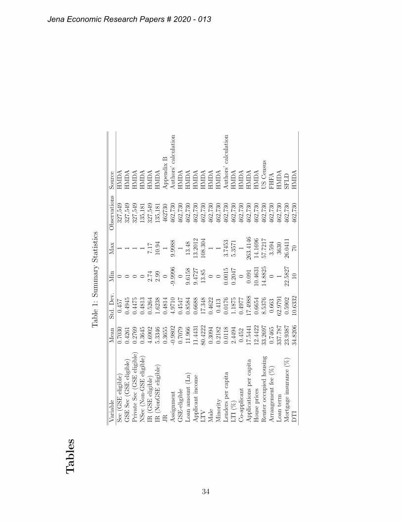
[Insert Table 1]
The other key dependent variable is IR, the loan’s interest rate at the point of
origination. We construct IR separately for GSE-eligible and non-GSE-eligible loans.
Table 1 shows that 70% of GSE eligible loans are securitized with 43% sold to a GSE
Veterans Association and the Federal Housing Administration. We exclude these observations onthe grounds that they are unconventional loans.
6Appendix Table A2 illustrates the geographical spread of the observations in the data set. Whilesome state borders contain more observations than others, there are typically thousands ofobservations in each state pair. It is therefore unlikely our findings are due to idiosyncrasiesof a limited number of states.
10
Jena Economic Research Papers # 2020 - 013

and 27% to a private buyer. 36% of non-GSE-eligible loans are securitized. The rate
of securitization in the data set is comparable to other recent studies (Bhutta, 2009;
Buchak et al., 2018). The mean interest rate on GSE-eligible and non-GSE-eligible
loans is 4.69% and 5.33%, respectively.
3.3 Explanatory Variables
The key explanatory variable is a dummy variable that captures the type of foreclosu-
re law used in the state where the property is located. We read the citations to
foreclosure law in each state’s constitution to ascertain which processes are available.
Next, we retrieve data from foreclosure auction listings on Realtytrac.com, Ghent
(2014), and interview attorneys to confirm our classification. Appendix C provides
this data. Figure 3 shows the type of law used in each state. We construct a JR
dummy variable that equals 1 if a property is in a JR state, 0 for PS states.
[Insert Figure 3]
As our empirical strategy relies on an RD design, we construct the assignment
variable using the distance between the midpoint of the property’s census tract and
the nearest JR-PS border coordinate.7 Following convention in the literature, the
assignment variable takes a negative value for observations in the control group (PS
states) and positive values for observations in the treatment group (JR states).
We merge the loan-level data with several additional variables from other sources.
To capture other characteristics of state law, we generate dummy variables for
whether a state allows right of redemption, deficiency judgments (Ghent and Kudlyak,
2011), the annual state homestead and non-homestead bankruptcy exemptions levels,
and retrieve a single-family home zoning restrictiveness index from Calder (2017).
7As census tracts are geographically small, the census tract midpoint is an accurate approximationof the property’s location.
11
Jena Economic Research Papers # 2020 - 013
We incorporate county-level information on the unemployment rate (Bureau of
Economic Analysis), the share of the population living in poverty (US Census), the
delinquency rate on automobile and credit card loans (NY Fed and CFPB), crime
rates (US Census), the share of the population with a college degree (US Census), the
average FICO score of borrowers at the point of origination, and the rate of successful
renegotiation on delinquent loans (SFLD).8 We approximate competition in the
local mortgage market using a county-level Herfindahl-Hirschman Index (HHI).9 The
FHFA provides census tract-level data on arrangement fees (the ratio of arrangement
fees to loan amount). We measure access to credit using the number of lender
branches per 1,000 population in each census tract. To capture credit demand we
use the number of mortgage applications per 1,000 population in each census tract.
We calculate the census tract-level mortgage refinancing rate as the ratio of mortgage
refinancing applications to total applications.
Finally, each HMDA loan provides an identifier for the originating institution
that is also present in Condition and Income Reports provided by the Federal Deposit
Insurance Corporation (FDIC). We therefore merge in bank-level data from this
source for the loans in the data set that are originated by banks.10 This allows us
to incorporate information on the bank’s size (the natural logarithm of assets), net
interest income ratio, Z-score, capital ratio, cost of deposits (the ratio of deposit
interest expenses to deposit liabilities), and an out of state dummy variable that
equals 1 if a loan is originated by a bank headquartered in state s to a borrower
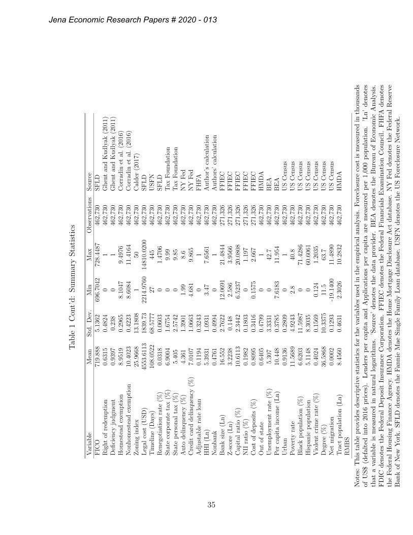
outside state s, 0 otherwise.11 Table 1 provides a list of the variables in the data
8The renegotiation rate is the percentage of mortgages that default and successfully renegotiateterms with the securitizer.
9We calculate the HHI index using lenders’ market shares where market share is the ratio of thetotal value of mortgage loans originated by lender l relative to the total value of mortgage loansoriginated by all institutions in the county. The HHI then is calculated as the sum of the squaresof the market shares of all financial institutions in each county.
10Non-deposit taking lenders that are present in the HMDA data do not appear in Call Reports.11The Z-score is calculated using the equation: Zl = (ROAl + ETAl)/ROASDl where ROAl,
12
Jena Economic Research Papers # 2020 - 013
set, summary statistics, and the source. Appendix B provides the definition of each
variable.
4 Identification Strategy and Diagnostic Tests
Our econometric strategy utilizes a parametric RD design. We estimate
yilrs = α + βJRs + γf(Xilrs) + ϕWilrs + δr + δl + εilrs, (1)
where yilrs is a dependent variable (either interest rates or a securitization indicator)
for loan i originated by lender l in region r of state s; JRs defines treatment status
and is equal to 1 if a property is in a JR state, 0 for PS states; f(Xilrs) contains
first-order polynomial expressions of the assignment variable and an interaction
between JRs and the assignment variable; Wilrs is a vector of control variables; εilrs
is the error term.
Equation (1) includes region fixed effects, δr. We define a region as an area 20
miles long by 10 miles wide that overlaps the threshold. As an example, Figure 4
illustrates the regions along a section of the Arkansas-Louisiana border. The region
fixed effects eliminate local and aggregate unobserved heterogeneity and also sharpen
identification. Specifically, the local average treatment effect (LATE) is computed
by comparing outcomes to the left and right of the threshold within the same region.
As the source of identification is confined to small, economically homogeneous areas
at the same point in time, omitted variables are unlikely to drive our inferences.
Focusing on regions close to the border is similar to the approach in Pence (2006)
who considers MSAs that overlap state borders.
ETAl, and ROASDl are return on assets, the ratio of equity to total assets, and the standarddeviation of returns on assets over the four quarters of 2018 for bank l, respectively.
13
Jena Economic Research Papers # 2020 - 013
[Insert Figure 4]
We also include lender fixed effects, δl. These capture all lender specific factors
such as risk preferences, managerial quality, or business models that may impact
securitization and pricing decisions. Lender fixed effects also purge cross-sectional
regulatory differences. For example, non-depository institutions (non-banks) are
regulated at the state level whereas domestic banks with national charters and
foreign banks are regulated by the OCC, while state chartered banks are supervised
by the state regulator in conjunction with the FDIC or Federal Reserve.
4.1 Exogeneity
Critical to our identification strategy is the exogeneity of foreclosure law. Ghent
(2014) reports that foreclosure law is exogenous with respect to contemporary econo-
mic conditions and lenders’ behavior because most states’ foreclosure law was determ-
ined by idiosyncratic factors during the pre-Civil War period. For example, the
original 13 states inherited JR law from England. PS law developed during the
early eighteenth century in response to British lenders asking courts to agree to a
sale-in-lieu of foreclosure. As the laws governing foreclosure were determined in case
law they have largely endured to the present day. This is because once there is
precedent, the law rarely changes substantially. Indeed, Ghent (2014) is explicit in
her assessment, stating,
“Given the extremely early date at which I find that foreclosure procedures were
established, it is safe to treat differences in some state mortgage laws, at least at
present, as exogenous, which may provide economists with a useful instrument for
studying the effect of differences in creditor rights.”
Other recent papers that treat foreclosure law as exogenous with respect to lender
behavior and contemporary economic matters include Pence (2006), Gerardi et al.
14
Jena Economic Research Papers # 2020 - 013
(2013), and Mian et al. (2015).
4.2 Diagnostic Checks
While treatment status is exogenous in equation (1), the validity of our econometric
strategy rests upon two identifying assumptions. First, all other pre-determined
factors that affect securitization and interest rates must be continuous functions
across the threshold. If this assumption is violated, estimates of β will capture both
the effect of JR law as well as the discontinuous factor leading to biased estimates.
Following convention in the literature, Table 2 presents t-tests that inspect
whether the balanced covariates assumption holds in our data. Panel A of Table 2
examines socioeconomic factors that are common irrespective of loan type between
the JR and PS regions. We find no significant differences in macroeconomic conditio-
ns (per capita income and unemployment), state tax rates, urbanization, the inciden-
ce of poverty, ethnic composition, and educational attainment. Housing markets are
strongly similar on either side of the threshold in terms of house prices, the share of
the housing stock that is rented, and zoning regulations. The rate of renegotiation
on delinquent mortgages and the rate of default on other types of debt are also
insignificantly different. The characteristics of financial intermediaries operating in
the regions are highly similar. For example, non-banks originate an equal share
of mortgages in JR and PS regions while banks have similar capital ratios and
Z-scores. There is no significant difference in the share of loans originated by banks
to borrowers outside their headquarter state.
Panel B in Table 2 presents results for a number of variables related to the
GSE-eligible loan sample. We find no significant differences between the treatment
and control groups in terms of applicant income, gender and ethnic composition of
borrowers, LTV and DTI ratios, term to maturity, mortgage insurance, and FICO
15
Jena Economic Research Papers # 2020 - 013
scores. While we have somewhat fewer variables available for non-GSE-eligible loans,
Panel C of Table 2 shows no significant differences in the characteristics of these loans
either side of the threshold.
[Insert Table 2] [Insert Table 3] [Insert Figure 5]
The second assumption is that neither borrowers nor lenders have precise control
over treatment status (Lee, 2008). This assumption is likely to hold because housing
availability and budget constraints prevent borrowers from perfectly choosing where
they live. We inspect this assumption using McCrary (2008)’s test for strategic
manipulation by estimating whether the density of mortgage applications and lender
branches per 1,000 population are continuous functions of the threshold. Manipulat-
ion by borrowers (lenders) would be consistent with a higher application (lender)
density within JR (PS) states. We estimate the equation
yc = α + βJRc + γXc + δr + εc, (2)
where yc is either the number of mortgage applications or lenders per 1,000 population
within census tract c; JRc is equal to 1 if an observation is from a JR state, 0
otherwise; Xc is a vector of control variables; δr are region fixed effects; εc is the
error term.12
The results of this test are presented in Table 3. We find no evidence of
strategic manipulation by either borrowers or lenders. Estimates of β are statistically
insignificant throughout columns 1 to 6 of Table 3, irrespective of whether we include
control variables, or estimate equation (2) parametrically or non-parametrically.
Panel A of Figure 5 presents corresponding graphical evidence showing the density
of loan applications is continuous across the threshold.
12We conduct these tests at the census tract level because we require information on the rate ofapplications or the density of lenders.
16
Jena Economic Research Papers # 2020 - 013
To further inspect whether borrowers manipulate treatment status we examine
net migration flows between US counties. Manipulation would be consistent with
significant inflows into JR counties. In column 7 of Table 3 we find no significant
differences in net migration to JR counties relative to PS counties. Another danger is
that borrowers try harder to obtain GSE-eligible status in JR states. However, Panel
B of Figure 5 shows no discontinuity in the GSE-eligible share of loan applications
at the threshold. The corresponding econometric test in column 8 of Table 3 shows
no significant effects.
5 Empirical Analysis
We begin by examining securitization and pricing patterns in the raw data at the
JR-PS threshold using non-parametric methods. Following Lee and Lemieux (2010)
we calculate the optimal bin width to be 0.4 miles, group the loan-level data into
bins, and fit local regression functions to the data on the left and right of the
threshold.13
[Insert Figure 6]
Figure 6 shows that JR law elicits heterogeneous securitization and pricing
responses across markets. Consistent with our hypotheses, we find in the GSE-eligible
market JR law causes a jump in the GSE securitization rate (Panel A) but not in
interest rates (Panel B), consistent with the CIRP preventing lenders from pricing
the credit risk of JR law into mortgage contracts. In the non-agency market, JR
law has no effect on securitization (Panel C) but increases interest rates (Panel D).
13The results are similar when we fit the local polynomial regressions using half and twice theoptimal bandwidth.
17
Jena Economic Research Papers # 2020 - 013
5.1 Securitization and Pricing Results
To pin down precise estimates of the LATE we turn to regression analysis. Column
1 of Table 4 presents linear regression estimates of equation (1) using GSE Sec as
the dependent variable. The LATE is estimated to be 0.0217 and is statistically
significant at the 1% level. This implies that JR law causes a 5.3% increase in the
probability that a mortgage loan is securitized, relative to the counterfactual.14
[Insert Table 4]
Among the control variables, we find securitization to be significantly negatively
correlated with applicant income and minority status. The probability of securitiza-
tion is significantly higher for high LTV loans and in areas with more lenders per
capita. Gender is an insignificant determinant of securitization. The assignment
variable, and its interaction with the JR indicator are statistically insignificant,
consistent with the relatively flat local regression functions shown in Panel A of
Figure 6.15
To ensure the findings are not a product of the linear probability model, we
estimate equation (1) using a logit model. The logit estimates in column 2 of Table
4 are similar to before.
The effects of JR law on securitization of non-GSE-eligible loans are quite different.
In columns 3 and 4 of Table 4 the JR law coefficient is insignificant, irrespective of
whether we estimate equation (1) using an OLS or logit model.
Lenders could also mitigate the credit risk of JR law by charging higher interest
rates. In the remainder of Table 4, we investigate whether JR law elicits pricing
14To calculate the treatment effect relative to the counterfactual we compare the LATE to themean rate of securitization within the control group which is 41%. Hence, (0.0217/0.41)*100 =5.3%.
15Appendix Table A6 shows that JR law has a similar effect on securitization of loans eligible forsale to Ginnie Mae.
18
Jena Economic Research Papers # 2020 - 013
effects across the two markets. We implement this test using the loan’s interest
rate as the dependent variable in equation (1). Column 5 of the table reports
estimates using the GSE-eligible sample. Consistent with the patterns in the raw
data, the JR coefficient is insignificant. In contrast, in the non-GSE-eligible market
JR law provokes significant pricing responses. The LATE in column 6 of Table 4
indicates the law causes interest rates to jump by 0.0823 percentage points (8.23
basis points) at the threshold. This is equivalent to a 1.7% increase relative to the
counterfactual.16
Residential mortgage backed securities (RMBS) provide another window into
the pricing effects of JR law. Intuitively, yields at issue on RMBS should be an
increasing function of the deal’s exposure to JR law as investors demand a premium
to hold a security with credit risk. To preserve space, details on the RMBS data
set and results are provided in Appendix E.2. Table A8 reports estimates that
relate a security’s initial yield to the JR share of the deal value. The table shows a
one percentage point increase in the JR share of the deal is associated with a 0.08
percentage point increase in the yield.
Together the evidence shows that in the GSE-eligible market the CIRP prevents
lenders from pricing credit risk due to JR law, which induces lenders to use securitiza-
tion to transfer credit risk to the GSEs. In the non-GSE-eligible market, purchasers
demand a premium for holding securities that have exposure to JR law. As private
purchasers also have incentives to minimize the costs of JR law, lenders cannot use
securitization to unload credit risk. Rather, informed parties adjust interest rates
to reflect the costs of JR law.
We conduct sensitivity checks to ensure our findings are not due to methodological
16Table A7 shows the findings are highly similar using data from the period 2000 to 2017. Wefocus on 2018 because earlier HMDA vintages did not include information on interest rates orother important loan characteristics. The 2000 to 2017 sample therefore relies on informationdrawn from multiple data sources.
19
Jena Economic Research Papers # 2020 - 013
considerations. Appendix Table A9 reports estimates from models with higher order
polynomial expressions of the assignment variable. Table A10 presents results using
5 and 2.5 mile bandwidths. In both tables the findings are similar to our baseline
estimates.
5.2 Private Securitization in the Agency Market
Lenders also have the option to sell GSE-eligible loans to private buyers. Unlike the
GSEs, private buyers provide no purchase guarantees but lenders’ pricing decisions
remain constrained by the CIRP. JR law therefore has potentially different effects on
private loan sales within the GSE-eligible market. We first ask how JR law affects
the likelihood that GSE-eligible loans are securitized, irrespective of the buyer’s
identity. In column 1 of Panel A in Table A11 JR law causes a 2.0% increase in
the probability of securitization, and the coefficient is significant at the 10% level.
The smaller LATE compared to the baseline result is consistent with the findings
in column 2 of Panel A showing JR law significantly decreases the probability that
a lender sells a GSE-eligible loan to a private institution.
A negative relationship between private securitization and JR law in the agency
market is consistent with our earlier results. The CIRP governs the pricing of
GSE-eligible loans regardless of whether a loan is subsequently securitized or the
buyer’s identity. When purchasing a GSE-eligible JR loan, private institutions
assume the credit risk of JR law without compensation through higher interest
rates. Private institutions are thus less willing to purchase a GSE-eligible loan if the
property is located in a JR state.17
17The negative relationship could be attributable to a higher probability that lenders successfullyrenegotiate terms with delinquent borrowers (Agarwal et al., 2011). Column 3 of Panel A inTable A11 shows this is not the case. Panel B in Table A11 shows our findings for securitizationin the GSE-eligible market are robust to using a multinomial logit estimator. Lenders may holdex ante information on whether a loan will be sold and the type of buyer. JR status could,in principle, therefore lead to higher interest rates on GSE-eligible loans where a lender wishes
20
Jena Economic Research Papers # 2020 - 013
5.3 Credit Risk Mechanism
Underpinning our tests is the hypothesis that JR law amplifies credit risk. We
therefore conduct sub-sample analyses to validate this mechanism. Intuitively, the
effects of JR law should be more pronounced within samples comprising riskier
borrowers where JR law has the largest effect on borrowers’ default incentives.
[Insert Table 5]
Panel A of Table 5 reports estimates of equation (1) for GSE-eligible securitization.
One would anticipate relatively larger LATEs among low versus high income borrowe-
rs. Credit risk increases with the DTI ratio as borrowers are more susceptible
to shocks that compromise their ability to meet mortgage payments. Similarly,
loans to borrowers with co-applicants are potentially less prone to default because
multiple income streams help smooth negative economic shocks. Consistent with
these conjectures, the estimates in columns 1 to 6 of Table 5 show the LATE is
larger for loans with income below relative to above the mean, for high relative to
low DTI loans, and for loans to sole relative to co-applicants.
In the remainder of Panel A, we split the sample based on socioeconomic conditio-
ns in the area where the property is located. In columns 7 and 8 we find that the
probability of securitization in response to JR law is substantially larger for loans
originated to borrowers who live in high relative to low unemployment areas. We
obtain similar results in columns 9 and 10 of the table when we split the sample
based on the poverty rate.
Panels B and C of Table 5 repeats the subsample tests for GSE-eligible interest
rates and non-GSE-eligible securitization, respectively. Consistent with the evidence
to make a loan attractive to a private buyer. Panel C of Table A11 refutes this conjecture.Irrespective of whether a loan is unsold (column 1) sold to a GSE (column 2) or private buyer(column 3), JR law has no effect on GSE-eligible interest rates. This is consistent with the CIRPpreventing foreclosure law-based pricing of GSE-eligible loans.
21
Jena Economic Research Papers # 2020 - 013

in Table 4, the LATE is statistically insignificant in all cells. Finally, Panel D
reports estimates for non-GSE-eligible interest rates. A consistent pattern emerges:
the LATE of JR law on interest rates is consistently larger among the riskier
subsamples.18
5.4 Which Channel Matters Most?
A key issue for policymakers is which margin of credit risk JR law influences.
Does JR law raise lenders’ legal costs during foreclosure, increase borrowers’ default
incentives, or both?
[Insert Table 6]
We therefore estimate equation (1) using the average state-level legal cost to
lenders and foreclosure timeline as control variables. The identifying assumption
in these tests is that legal costs and timelines vary exogenously. This appears
plausible as both variables are functions of exogenous foreclosure law. To enable
comparability of economic magnitudes we use standardized legal cost and timeline
variables. Column 1 in Table 6 shows a standard deviation increase in lenders’ legal
costs of foreclosure leads to a 0.10% increase in the probability that a GSE-eligible
loan is securitized, but the coefficient is insignificant. However, GSE-eligible securiti-
zation is more responsive to increasing the foreclosure timeline. The standardized
timeline coefficient is equivalent to a 1.61% increase in the probability of securitizati-
on. In column 2 of Table 6 we find a standard deviation increase in legal costs raises
non-GSE-eligible interests by 3.13% whereas increasing the foreclosure timeline by
18We also follow the approach used by Agarwal et al. (2012) to calculate the predicted probabilityof default for each loan. We then split the sample according to whether the probability of defaultlies above or below the mean. The results in Appendix Table A12 show that the JR coefficientis positive and statistically significant in both subsamples for GSE-eligible securitization andnon-GSE-eligible interest rates. However, in both cases, the effect of JR law is more pronouncedfor loans with default probabilities above the mean.
22
Jena Economic Research Papers # 2020 - 013
a standard deviation leads to 7.93% higher interest rates. Both coefficients are
significant at conventional levels.
Hence, while both aspects of JR law contribute to credit risk, the effect of the
law on securitization and intereste rates is primarily transmitted through borrower
moral hazard. JR law extends the foreclosure timeline which increases the returns
to default. Initiatives that speed up court procedures and shorten the foreclosure
process may help mitigate the distorting effects of JR law on credit markets.
6 Robustness Checks
In this section, we conduct sensitivity checks to rule out confounding factors.
6.1 Placebo Tests
A concern is that the relationship between the outcome variables and foreclosure
law is discontinuous at the threshold due to jumps in other factors. Placebo tests
provide insights into whether JR law drives the behavior we observe in the data.
Specifically, in samples where foreclosure law is continuous across the threshold, we
should not observe discontinuities in securitization or interest rates. We therefore
estimate the equation
yilrs = βP lacebos + γf(Dilrs) + ϕWilrs + δr + δl + εilrs, (3)
where all variables are the same as in equation (1) except Placebos which is a
dummy variable equal to 1 on the right of the placebo threshold, 0 on the left of the
placebo threshold; and Dilrs contains the distance to the placebo threshold and an
interaction between the placebo assignment variable and Placebos.
We first estimate equation (3) using observations within 10 miles of a placebo
23
Jena Economic Research Papers # 2020 - 013
threshold located 10 miles to the right of the actual threshold where JR law governs
the foreclosure process on both sides. The results reported in Panel A of Table 7
show the placebo coefficient is statistically insignificant throughout all specifications.
Neither the likelihood of securitization nor interest rates in the agency and non-agency
markets are discontinuous at the placebo threshold. Next, we repeat the procedure
using observations within 10 miles of a placebo threshold 10 miles to the left of
the actual threshold, where PS law regulates the foreclosure process either side. In
Panel B of Table 7 the placebo LATEs are again statistically insignificant.
[Insert Table 7]
To affirm our baseline estimates do not simply capture border effects, other
aspects of the legal environment, or political economy considerations, we use samples
drawn around the border between states that use the same foreclosure law. We
randomly assign states to placebo treatment and placebo control status and estimate
equation (3). Panel C (D) of Table 7 provides results from JR-JR (PS-PS) borders.
The placebo coefficient estimate is again statistically insignificant.
If an omitted variable drives our main findings, the placebo LATEs should be
similar in magnitude and statistical significance as the baseline estimates. Througho-
ut Table 7 this is not the case. That securitization and interest rates only jump at
the actual threshold where there exist discontinuities in the law governing foreclosure
reinforces our argument that the effects we observe are not driven by observable or
unobservable omitted variables.
6.2 The Legal Environment
Next, we ask whether other aspects of the state-level legal environment confound our
inferences. For example, right of redemption (ROR) law allows borrowers to redeem
24
Jena Economic Research Papers # 2020 - 013
their property within 12 months of foreclosure, potentially amplifying lenders’ costs.
Lenders may pursue delinquent borrowers’ future income to cover unpaid foreclosure
debts using deficiency judgments. Prior research documents a link between mortgage
default and bankruptcy exemptions (Lin, 2001).19 Zoning restrictions may also
influence lenders’ choices (Gyourko et al., 2019).
[Insert Table 8]
We therefore append equation (1) with controls for whether a state has ROR
law, allows deficiency judgments, homestead and nonhomestead exemptions, and
the single-family home zoning restrictiveness index. Throughout Panels A and B of
Table 8 our inferences endure.20
6.3 Lending Industry Conditions
Approximately half the loans in our sample are originated by banks with the remain-
der supplied by non-banks. Non-banks typically rely on short-term wholesale market
funding and are thus more likely to securitize loans to ensure repayment (Loutskina
19Homestead exemptions are the most important bankruptcy exemption and evidence shows thatmortgage default is more likely the more generous are homestead exemptions (Lin, 2001).Nonhomestead exemptions allow individuals to maintain wealth in other asset categories buttend to be set at low levels. For example, the mean homestead exemption across US states is$122,754 whereas the mean nonhomestead exemption (comprising automobile, other property(clothing, jewelry, and tools), and wildcard exemptions) is $19,685.
20Appendix Table A13 presents further legal robustness tests. We test the sensitivity of ourfindings to 1) excluding observations from Delaware and Pennsylvania which use scire facias,a creditor-friendly form of JR law (scire facias places the onus on the borrower to provide areason why the lender should not be able to foreclose (Ghent, 2014). Despite its perceivedcreditor-friendly nature, scire facias is neither expedient nor cheap for lenders. Data from theFannie Mae Single Family Loan database show the foreclosure timeline is longer and averageforeclosure cost to lenders is higher in Delaware and Pennsylvania relative to other JR states(see Appendix Table A4).) 2) excluding Texas as it is the only state that limits the LTV ratio ofmortgages to 80%, 3) excluding Louisiana from the sample on the grounds that it is the only CivilLaw state, and 4) excluding Massachusetts which undertook reforms to speed up the foreclosuretimeline during earlier years (Gerardi et al., 2013). Throughout Panels A and B of Table A13,the JR law coefficient remains robust despite these changes.
25
Jena Economic Research Papers # 2020 - 013
and Demyanyk, 2016; Buchak et al., 2018). To avoid that our findings reflect a
higher concentration of different lender types either side of the threshold, we split
the sample and estimate equation (1) using non-banks and banks separately. The
results in Table 9 show that JR law has a positive and statistically significant effect
on the probability of GSE securitization within both sub-samples. Both types of
financial intermediary respond to JR law by setting significantly higher interest rates
on non-GSE-eligible loans.
[Insert Table 9]
Next, we examine the sensitivity of our findings to conditions within the banking
industry. Bank characteristics such as size, profitability, soundness, and capitalizati-
on may influence securitization and pricing decisions. Theory and evidence shows
the cost of deposits affects how banks fund loans (Pennacchi, 1988; Gorton and
Pennacchi, 1995; Loutskina and Strahan, 2009). In addition, banks may lend across
state borders. If a state regulator is more lenient on out-of-state activities compared
to lending at home (Ongena et al., 2013), this may pose a problem if the PS state
is more often the home state and the regulator dislikes the OTD model at home.
Banks are subject to different regulators depending on their charter. The estimates
in columns 1 to 5 and 7 to 11 of Table A14 allay these concerns.21
Next, we check whether the nature of banks’ business models drives our results.
A concern is that banks operating originate-to-distribute (OTD) models are highly
dependent on selling loans. If such institutions are disproportionately clustered on
the JR side of the threshold, our estimates will conflate banks’ business models with
the effect of JR law. To address this concern we focus exclusively on banks that do
not operate an OTD model, defined as banks that securitize less than 50% of the
21We must exclude the lender fixed effects from equation (1) to include the bank-level controlvariables.
26
Jena Economic Research Papers # 2020 - 013
mortgage loans they originate. The results in columns 6 and 12 of Table A14 are
very similar to before.
6.4 Loan Quality
A natural question is whether the LATEs capture differences in the characteristics
of borrowers or loans either side of the threshold. While the estimating equation
already includes covariates to capture such factors, we add further controls for the
LTI ratio, DTI ratio, term to maturity, house prices, the average FICO score, and
share of borrowers with mortgage insurance in the county the property is located.
Despite including these controls, in column 1 of Table 10 we continue to find JR law
elicits a significant increase in the securitization of GSE-eligible loans. In column 2
of the table the JR law coefficient is insignificant when GSE-eligible interest rates
is the dependent variable. Data constraints prevent us from including the FICO
and mortgage insurance variables in the corresponding tests using non-GSE-eligible
loans. However, in columns 3 and 4 of Table 10 our key findings are robust.
[Insert Table 10]
6.5 Miscellaneous Sensitivity Checks
We conduct additional robustness tests to rule out further threats to identification.
For brevity we report the estimates in Appendix Table A15. We append equation
(1) with controls for delinquency rates on auto and credit card loans to capture
differences in the general riskiness of the population. In addition, we control for the
renegotiation rate on delinquent mortgages to ensure the estimates do not capture
potential differences in borrowers’ propensity to self cure in JR states due to the
longer foreclosure timeline. As lenders’ profitability expectations are influenced by
pre-payment risk and changes in interest rates we control for the refinancing rate and
27
Jena Economic Research Papers # 2020 - 013
whether a loan has an adjustable interest rate. Han et al. (2015) report evidence
that tax rates can motivate securitization. The findings reported in Table A15
demonstrate our findings are stable despite adding these controls.
Finally, in Table A16 we sequentially focus on specific US regions to ensure local
conditions do not drive our inferences. Panel A (B) of the table reports estimates
using observations from the most (least) populous border regions. In Panels C to
G of Table A16 we focus on samples drawn from within the Northeast, Midwest,
West, and Southern states. Our findings remain remarkably stable. Only in the
Western subsample are the LATEs insignificant, although this is mainly due to the
small sample size.
7 Conclusions
We show that financial institutions manage credit risk stemming from JR law using
securitization or loan pricing. In the agency market, lenders exhibit an excessive
propensity to securitize loans to mitigate credit risk. This behavior stems from the
GSEs’ CIRP and implicit federal guarantees that create incentives for lenders to
unload credit risk to the GSEs rather than price credit risk into mortgage contracts.
In contrast, in the non-agency market lenders set higher interest rates to cover
expected losses because secondary market participants also have loss avoidance
incentives.
These findings have policy implications. Legislators have proposed changes to the
GSEs’ CIRP and purchase guarantees in the Corker-Warner 2013 and Johnson-Crapo
2014 Senate Bills. At heart, these efforts aim to reduce the GSEs’ debt holdings
and lower mortgage market costs to taxpayers. We show that lenders strategically
transfer loans worth approximately $79.5 billion to the GSEs each year because of
the credit risk JR law embodies. Ultimately, the GSEs absorb losses that accrue
28
Jena Economic Research Papers # 2020 - 013
on these loans, which happens more often compared to PS loans. Tackling these
issues may involve reforming the GSEs’ policies or introducing private capitalization.
However, our findings demonstrate that policy interventions that speed up judicial
procedures may help limit the credit risk JR law creates by resolving moral hazard
among borrowers.
Second, after 4 million homes were improperly foreclosed during the US Foreclosu-
re Crisis of 2010 to 2012, policy initiatives have sought to extend greater protections
to borrowers including introducing JR law in all states. Our research illustrates such
measures involve a trade-off. Protecting borrowers’ rights imposes greater credit risk
on lenders but for GSE-eligible loans the costs are borne by taxpayers.
Finally, the mechanism highlighted in this paper has implications for the design
of any secondary market where risk transfer incentives exist. A notable example
is the European Union’s STS market. The 2019 Securitization Regulation aims
to integrate European capital markets by assigning STS labels to deals where the
underlying assets are safe and transparent. The STS label specifies a set of criteria
assets must conform to but does not take into account the country in which the
loans are originated despite observable differences in credit risk across European
countries. This raises the possibility that STS deals are mispriced which creates
moral hazard within lenders and exposes purchasers to losses.
The mechanisms we document are potentially present in all secondary markets
for loan sales. Studying how lenders mitigate credit risk in these environments is an
exciting avenue for future research.
References
Agarwal, S., Amromin, G., Ben-David, C., Chomsisengphet, S., and Evanoff, D.
(2011). The role of securitization in mortgage renegotiation. Journal of Financial
29
Jena Economic Research Papers # 2020 - 013
Economics, 102(3):559–578.
Agarwal, S., Chang, Y., and Yavas, A. (2012). Adverse selection in mortgage
securitization. Journal of Financial Economics, 105(3):640–660.
Ahnert, T. and Kuncl, M. (2020). Loan insurance, market liquidity, and lending
standards. CEPR Working Paper.
Bhutta, N. (2009). Gse activity and mortgage supply in lower-income and minority
neighborhoods: The effect of the affordable housing goals. Federal Reserve
Working Paper 2009-03.
Bhutta, N. and Keys, B. (2018). Eyes wide shut? the moral hazard of mortgage
insurance during the housing boom. NBER Working Paper No. 24844.
Buchak, G., Matvos, G., Poskorski, T., and Seru, A. (2018). The limits of shadow
banks. NBER Working Paper 25149.
Calder, V. (2017). Zoning, land-use planning, and housing affordability. Cato
Institute Policy Analysis No. 823.
Clauretie, T. and Herzog, T. (1990). The effect of state foreclosure laws on loan
losses: Evidence from the mortgage industry. Journal of Money, Credit and
Banking, 22(2):221–233.
Corradin, S., Gropp, R., Huizinga, H., and Laeven, L. (2016). The effect of personal
bankruptcy exemptions on investment in home equity. Journal of Financial
Intermediation, 25:77–98.
Dagher, J. and Sun, Y. (2016). Borrower protection and the supply of credit:
Evidence from foreclosure laws. Journal of Financial Economics, 121(1):195–209.
30
Jena Economic Research Papers # 2020 - 013
Demiroglu, C., Dudley, E., and James, C. M. (2014). State foreclosure laws and the
incidence of mortgage default. Journal of Law and Economics, 57(1):225–280.
Elenev, V., Landvoigt, T., and Van Nieuwerburgh, S. (2016). Phasing out the GSEs.
Journal of Monetary Economics, 81(C):111–132.
Gerardi, K., Lambie-Hanson, L., and Willen, P. (2013). Do borrower rights improve
borrower outcomes? Evidence from the foreclosure process. Journal of Urban
Economics, 73(1):1–17.
Gete, P. and Zecchetto, F. (2018). Distributional implications of government
guarantees in mortgage markets. Review of Financial Studies, 31(3):1064–1097.
Ghent, A. (2014). How do case law and statute differ? Lessons from the evolution
of mortgage law. Journal of Law and Economics, 57(4):1085–1122.
Ghent, A. C. and Kudlyak, M. (2011). Recourse and residential mortgage default:
Evidence from US states. Review of Financial Studies, 124(9):3139–3186.
Gorton, G. and Pennacchi, G. (1995). Banks and loan sales marketing
nonmarketable assets. Journal of Monetary Economics, 35(3):389–411.
Gyourko, J., Hartley, J., and Krimmel, K. (2019). The local residential land
use regulatory environment across U.S. housing markets: Evidence from a new
wharton index. NBER Working Paper No. 26573.
Han, J., Park, K., and Pennacchi, G. (2015). Corporate taxes and securitization.
Journal of Finance, 70(3):1287–1321.
Hurst, E., Keys, B., Seru, A., and Vavra, J. (2016). Regional redistribution through
the U.S. mortgage market. American Economic Review, 106(10):2989–3028.
31
Jena Economic Research Papers # 2020 - 013
Kahn, J. and Kay, B. (2019). The impact of credit risk mispricing on mortgage
lending during the subprime boom. BIS Working Paper.
Keys, B., Mukherjee, T., Seru, A., and Vig, V. (2010). Did securitization lead to
lax screening? Evidence from subprime loans. Quarterly Journal of Economics,
125(1):307–362.
Keys, B., Seru, A., and Vig, V. (2012). Lender screening and the role of
securitization: Evidence from prime and subprime mortgage markets. Review
of Financial Studies, 25(7):2071–2108.
Lee, D. (2008). Randomized experiments from non-random selection in U.S. house
elections. Journal of Econometrics, 142(2):675–697.
Lee, D. S. and Lemieux, T. (2010). Regression discontinuity designs in economics.
Journal of Economic Literature, 48(2):281–355.
Lin, E.Y. White, M. (2001). Bankruptcy and the market for mortgage and home
improvement loans. Journal of Urban Economics, 50(1):138–162.
Loutskina, E. (2011). The role of securitization in bank liquidity and funding
management. Journal of Financial Economics, 100(3):663–684.
Loutskina, E. and Demyanyk, Y. (2016). Mortgage companies and regulatory
arbitrage. Journal of Financial Economics, 122(2):328–351.
Loutskina, E. and Strahan, P. (2009). Securitization and the declining impact of
bank financial condition on loan supply: Evidence from mortgage originations.
Journal of Finance, 64(2):861–922.
McCrary, J. (2008). Manipulation of the running variable in the regression
discontinuity design: A density test. Journal of Econometrics, 142(2):698–714.
32
Jena Economic Research Papers # 2020 - 013
Melzer, B. T. (2017). Mortgage debt overhang: Reduced investment by homeowners
at risk of default. Journal of Finance, 72(2):575–612.
Mian, A., Sufi, A., and Trebbi, F. (2015). Foreclosures, house prices, and the real
economy. Journal of Finance, 70(6):2587–2634.
Ongena, S., Popov, A., and Udell, G. (2013). When the cat’s away the mice will play:
Does regulation at home affect bank risk-taking abroad? Journal of Financial
Economics, 108(3):727–750.
Parlour, C. and Winton, A. (2013). Laying off credit risk: Loan sales versus credit
default swaps. Journal of Financial Economics, 107(1):25–45.
Pence, K. M. (2006). Foreclosing on opportunity: State laws and mortgage credit.
Review of Economics and Statistics, 88(1):177–182.
Pennacchi, G. (1988). Loan sales and the cost of bank capital. Journal of Finance,
43:375–396.
Piskorski, T., Seru, A., and Vig, V. (2010). Securitization and distressed loan
renegotiation: Evidence from the subprime mortgage crisis. Journal of Financial
Economics, 97(3):369–397.
Purnanandam, A. (2010). Originate-to-distribute model and the subprime mortgage
crisis. Review of Financial Studies, 24(6):1881–1915.
Schill, M. (1991). An economic analysis of mortgagor protection laws. Virginia Law
Review, 77(3):489–538.
Seiler, M., Seiler, V., Lane, M., and Harrison, D. (2012). Fear, shame and guilt:
Economic and behavioral motivations for strategic default. Real Estate Economics,
40(1):199–233.
33
Jena Economic Research Papers # 2020 - 013
Tab
les
Tab
le1:
Sum
mar
ySta
tist
ics
Var
iable
Mea
nStd
.D
ev.
Min
Max
Obse
rvat
ions
Sou
rce
Sec
(GSE
elig
ible
)0.
7030
0.45
70
132
7,54
9H
MD
AG
SE
Sec
(GSE
elig
ible
)0.
4261
0.49
450
132
7,54
9H
MD
AP
riva
teSec
(GSE
elig
ible
)0.
2769
0.44
750
132
7,54
9H
MD
AN
Sec
(Non
-GSE
elig
ible
)0.
3645
0.48
130
113
5,18
1H
MD
AIR
(GSE
elig
ible
)4.
6902
0.52
642.
747.
1732
7,54
9H
MD
AIR
(Non
GSE
elig
ible
)5.
3346
1.62
382.
9910
.94
135,
181
HM
DA
JR
0.36
550.
4814
01
4627
30A
pp
endix
BA
ssig
nm
ent
-0.9
802
4.97
10-9
.999
69.
9988
462,
730
Auth
ors’
calc
ula
tion
GSE
-eligi
ble
0.70
790.
4547
01
462,
730
HM
DA
Loa
nam
ount
(Ln)
11.9
660.
8584
9.61
5813
.48
462,
730
HM
DA
Applica
nt
inco
me
11.4
431
0.66
889.
4727
13.2
012
462,
730
HM
DA
LT
V80
.422
217
.348
13.8
510
8.30
446
2,73
0H
MD
AM
ale
0.30
940.
4622
01
462,
730
HM
DA
Min
orit
y0.
2182
0.41
30
146
2,73
0H
MD
AL
ender
sp
erca
pit
a0.
0118
0.01
760.
0015
3.74
5346
2,73
0A
uth
ors’
calc
ula
tion
LT
I(%
)2.
4494
1.18
750.
2047
5.35
7146
2,73
0H
MD
AC
o-ap
plica
nt
0.45
20.
4977
01
462,
730
HM
DA
Applica
tion
sp
erca
pit
a17
.544
117
.498
80.
091
263.
4146
462,
730
HM
DA
Hou
sepri
ces
12.4
422
0.66
5410
.463
114
.169
646
2,73
0H
MD
AR
ente
rocc
upie
dhou
sing
33.2
697
8.53
7614
.882
557
.721
746
2,73
0U
SC
ensu
sA
rran
gem
ent
fee
(%)
0.74
650.
663
03.
594
462,
730
FH
FA
Loa
nte
rm33
7.78
762
.979
11
3630
462,
730
HM
DA
Mor
tgag
ein
sura
nce
(%)
23.9
387
0.59
0222
.582
726
.041
146
2,73
0SF
LD
DT
I34
.820
610
.633
210
7046
2,73
0H
MD
A
34
Jena Economic Research Papers # 2020 - 013
Tab
le1
Con
t’d:
Sum
mar
ySta
tist
ics
Var
iable
Mea
nStd
.D
ev.
Min
Max
Obse
rvat
ions
Sou
rce
FIC
O71
9.88
85.
1362
696.
7042
728.
4487
462,
730
SF
LD
Rig
ht
ofre
dem
pti
on0.
6315
0.48
240
146
2,73
0G
hen
tan
dK
udly
ak(2
011)
Defi
cien
cyju
dgm
ent
0.93
970.
238
01
462,
730
Ghen
tan
dK
udly
ak(2
011)
Hom
este
adex
empti
on8.
9519
0.29
658.
1047
9.49
7646
2,73
0C
orra
din
etal
.(2
016)
Non
hom
este
adex
empti
on10
.402
30.
4223
8.60
8411
.416
446
2,73
0C
orra
din
etal
.(2
016)
Zon
ing
index
25.9
668
13.1
808
150
462,
730
Cal
der
(201
7)L
egal
cost
(USD
)45
53.6
113
1839
.73
2214
.976
014
810.
0200
462,
730
SF
LD
Tim
elin
e(D
ays)
108.
0522
68.5
777
2744
546
2,73
0U
SF
NR
eneg
otia
tion
rate
(%)
0.03
180.
0603
01.
4706
462,
730
SF
LD
Sta
teco
rpor
ate
tax
(%)
6.90
041.
6754
09.
9946
2,73
0T
axF
oundat
ion
Sta
tep
erso
nal
tax
(%)
5.40
52.
5742
09.
8546
2,73
0T
axF
oundat
ion
Auto
del
inquen
cy(%
)4.
361
1.39
011.
998.
646
2,73
0N
YF
edC
redit
card
del
inquen
cy(%
)7.
0107
1.06
634.
681
9.86
546
2,73
0N
YF
edA
dju
stab
lera
telo
an0.
1194
0.32
430
146
2,73
0F
HFA
HH
I(L
n)
5.39
311.
0931
3.47
7.65
6146
2,73
0A
uth
or’s
calc
ula
tion
Non
ban
k0.
4761
0.49
940
146
2,73
0A
uth
ors’
calc
ula
tion
Ban
ksi
ze(L
n)
16.5
522.
7622
12.0
691
21.4
844
271,
326
FF
IEC
Z-s
core
(Ln)
3.22
380.
148
2.58
63.
9566
271,
326
FF
IEC
Cap
ital
rati
o(%
)10
.611
32.
3442
6.52
3720
.080
827
1,32
6F
FIE
CN
IIra
tio
(%)
0.19
820.
1803
01.
197
271,
326
FF
IEC
Cos
tof
dep
osit
s(%
)0.
8095
0.34
160.
1575
2.66
727
1,32
6F
FIE
CO
ut
ofst
ate
0.64
050.
4799
01
462,
730
HM
DA
Unem
plo
ym
ent
rate
(%)
5.30
73.
3331
042
.746
2,73
0B
EA
Per
capit
ain
com
e(L
n)
10.4
480.
3785
7.61
8311
.954
462,
730
BE
AU
rban
0.91
360.
2809
01
462,
730
US
Cen
sus
Pov
erty
rate
11.5
689
4.92
432.
840
.846
2,73
0U
SC
ensu
sB
lack
pop
ula
tion
(%)
6.62
0311
.598
70
71.4
286
462,
730
US
Cen
sus
His
pan
icp
opula
tion
5.11
488.
3035
060
.606
146
2,73
0U
SC
ensu
sV
iole
nt
crim
era
te(%
)0.
4024
0.15
690.
124
1.20
3546
2,73
0U
SC
ensu
sD
egre
e(%
)36
.586
810
.337
511
.563
.746
2,73
0U
SC
ensu
sN
etm
igra
tion
0.00
020.
1293
-19.
1400
11.4
890
462,
730
US
Cen
sus
Tra
ctp
opula
tion
(Ln)
8.45
600.
4631
2.30
2610
.283
246
2,73
0H
MD
AR
MB
S
Not
es:
Th
ista
ble
pro
vid
esd
escr
ipti
vest
atis
tics
for
the
vari
able
su
sed
inth
eem
pir
ical
anal
ysi
s.F
orec
losu
reco
stis
mea
sure
din
thou
san
ds
ofU
S$
(def
alte
din
to20
16pri
ces)
.L
end
ers
per
cap
ita
and
Ap
pli
cati
ons
per
cap
ita
are
mea
sure
dp
er1,
000
pop
ula
tion
.’L
n’
den
otes
that
ava
riab
leis
mea
sure
din
nat
ura
llo
gari
thm
s.’S
ourc
e’d
enot
esth
ed
ata
pro
vid
er.
BE
Ad
enot
esth
eB
ure
auof
Eco
nom
icA
nal
ysi
s.F
DIC
den
otes
the
Fed
eral
Dep
osit
Insu
ran
ceC
orp
orat
ion
.F
FIE
Cd
enot
esth
eF
eder
alF
inan
cial
sE
xam
inat
ion
Cou
nci
l.F
HFA
den
otes
the
Fed
eral
Hou
sin
gF
inan
ceA
gen
cy.
HM
DA
den
otes
the
Hom
eM
ortg
age
Dis
clos
ure
Act
dat
abas
e.N
YF
edd
enot
esth
eF
eder
alR
eser
veB
ank
ofN
ewY
ork.
SF
LD
den
otes
the
Fan
nie
Mae
Sin
gle
Fam
ily
Loa
nd
atab
ase.
US
FN
den
otes
the
US
For
eclo
sure
Net
wor
k.
35
Jena Economic Research Papers # 2020 - 013
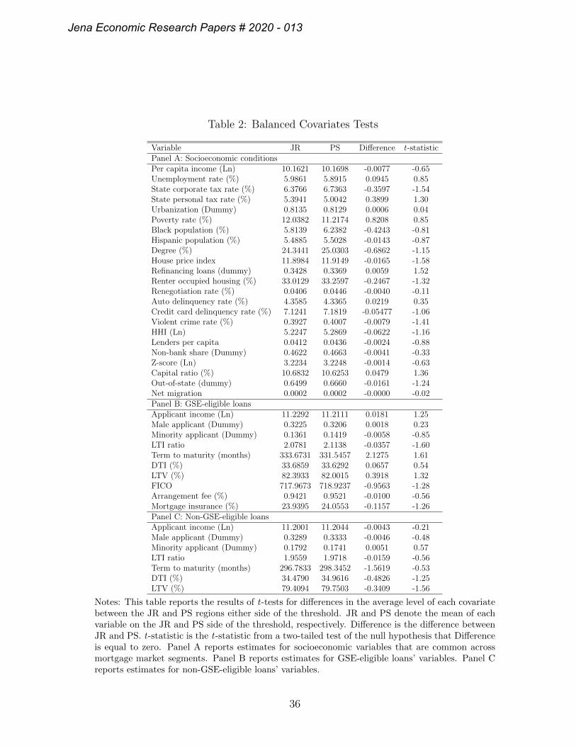
Table 2: Balanced Covariates Tests
Variable JR PS Difference t-statisticPanel A: Socioeconomic conditionsPer capita income (Ln) 10.1621 10.1698 -0.0077 -0.65Unemployment rate (%) 5.9861 5.8915 0.0945 0.85State corporate tax rate (%) 6.3766 6.7363 -0.3597 -1.54State personal tax rate (%) 5.3941 5.0042 0.3899 1.30Urbanization (Dummy) 0.8135 0.8129 0.0006 0.04Poverty rate (%) 12.0382 11.2174 0.8208 0.85Black population (%) 5.8139 6.2382 -0.4243 -0.81Hispanic population (%) 5.4885 5.5028 -0.0143 -0.87Degree (%) 24.3441 25.0303 -0.6862 -1.15House price index 11.8984 11.9149 -0.0165 -1.58Refinancing loans (dummy) 0.3428 0.3369 0.0059 1.52Renter occupied housing (%) 33.0129 33.2597 -0.2467 -1.32Renegotiation rate (%) 0.0406 0.0446 -0.0040 -0.11Auto delinquency rate (%) 4.3585 4.3365 0.0219 0.35Credit card delinquency rate (%) 7.1241 7.1819 -0.05477 -1.06Violent crime rate (%) 0.3927 0.4007 -0.0079 -1.41HHI (Ln) 5.2247 5.2869 -0.0622 -1.16Lenders per capita 0.0412 0.0436 -0.0024 -0.88Non-bank share (Dummy) 0.4622 0.4663 -0.0041 -0.33Z-score (Ln) 3.2234 3.2248 -0.0014 -0.63Capital ratio (%) 10.6832 10.6253 0.0479 1.36Out-of-state (dummy) 0.6499 0.6660 -0.0161 -1.24Net migration 0.0002 0.0002 -0.0000 -0.02Panel B: GSE-eligible loansApplicant income (Ln) 11.2292 11.2111 0.0181 1.25Male applicant (Dummy) 0.3225 0.3206 0.0018 0.23Minority applicant (Dummy) 0.1361 0.1419 -0.0058 -0.85LTI ratio 2.0781 2.1138 -0.0357 -1.60Term to maturity (months) 333.6731 331.5457 2.1275 1.61DTI (%) 33.6859 33.6292 0.0657 0.54LTV (%) 82.3933 82.0015 0.3918 1.32FICO 717.9673 718.9237 -0.9563 -1.28Arrangement fee (%) 0.9421 0.9521 -0.0100 -0.56Mortgage insurance (%) 23.9395 24.0553 -0.1157 -1.26Panel C: Non-GSE-eligible loansApplicant income (Ln) 11.2001 11.2044 -0.0043 -0.21Male applicant (Dummy) 0.3289 0.3333 -0.0046 -0.48Minority applicant (Dummy) 0.1792 0.1741 0.0051 0.57LTI ratio 1.9559 1.9718 -0.0159 -0.56Term to maturity (months) 296.7833 298.3452 -1.5619 -0.53DTI (%) 34.4790 34.9616 -0.4826 -1.25LTV (%) 79.4094 79.7503 -0.3409 -1.56
Notes: This table reports the results of t-tests for differences in the average level of each covariatebetween the JR and PS regions either side of the threshold. JR and PS denote the mean of eachvariable on the JR and PS side of the threshold, respectively. Difference is the difference betweenJR and PS. t-statistic is the t-statistic from a two-tailed test of the null hypothesis that Differenceis equal to zero. Panel A reports estimates for socioeconomic variables that are common acrossmortgage market segments. Panel B reports estimates for GSE-eligible loans’ variables. Panel Creports estimates for non-GSE-eligible loans’ variables.
36
Jena Economic Research Papers # 2020 - 013
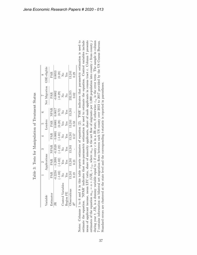
Tab
le3:
Tes
tsfo
rM
anip
ula
tion
ofT
reat
men
tSta
tus
12
34
56
78
Var
iable
Applica
tion
sL
ender
sN
etM
igra
tion
GSE
-eligi
ble
Est
imat
orP
AR
PA
RN
PA
RP
AR
PA
RN
PA
RP
AR
PA
RJR
-0.2
234
-0.
2091
-0.3
520
-0.
0001
0.00
010.
0017
-0.0
002
0.00
53(-
1.03
)(-
1.02
)(-
1.22
)(-
1.01
)(0
.28)
(0.7
2)(-
0.29
)(0
.28)
Con
trol
Var
iable
sN
oY
esN
oN
oY
esN
oN
oN
oR
egio
nF
EY
esY
esY
esY
esY
esY
esN
oY
esO
bse
rvat
ions
13,2
4113
,241
13,2
4113
,241
13,2
4113
,241
232,
315
13,2
41R
20.
190.
21-
0.57
0.58
-0.
020.
29
Not
es:
Col
um
ns
1to
6an
d8
inth
ista
ble
rep
orts
esti
mat
esof
equ
atio
n(2
).’P
AR
’in
dic
ates
that
par
amet
ric
esti
mat
ion
isu
sed
toes
tim
ate
the
equ
atio
n.
’NP
AR
’in
dic
ate
sth
atn
on-p
aram
etri
ces
tim
atio
nis
use
dto
esti
mat
eth
eeq
uat
ion
.C
ontr
olva
riab
les
incl
ud
em
ean
ofap
pli
cant
inco
me,
mea
nLT
Cra
tio,
shar
eof
min
orit
yap
pli
cants
,sh
are
ofm
ale
app
lica
nts
ince
nsu
str
actc.
Col
um
n7
pre
sents
esti
mat
esof
the
equ
ati
onm
cj
=α
+βJR
c+ε c
j,
wh
erem
cj
isth
en
etfl
owof
mig
rants
per
1,00
0p
opu
lati
onin
toco
untyc
from
cou
ntyj
du
rin
gye
art;JR
cis
ad
um
my
vari
able
equal
to1
ifco
untyc
isin
aJR
stat
e,0
oth
erw
ise;ε c
jis
the
erro
rte
rm.
Th
esa
mp
lein
colu
mn
7co
nta
ins
info
rmat
ion
onb
ilat
eral
net
mig
rati
onfl
ows
bet
wee
nea
chU
Sco
unty
over
2013
to20
17p
rovid
edby
the
US
Cen
sus
Bu
reau
.S
tan
dar
der
rors
are
clu
ster
edat
the
stat
ele
vel
and
the
corr
esp
ond
ingt-
stat
isti
cis
rep
orte
din
par
enth
eses
.
37
Jena Economic Research Papers # 2020 - 013
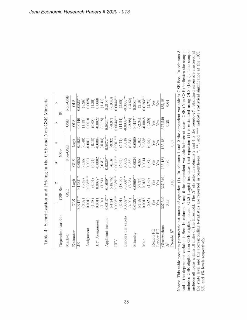
Tab
le4:
Sec
uri
tiza
tion
and
Pri
cing
inth
eG
SE
and
Non
-GSE
Mar
kets
12
34
56
Dep
enden
tva
riab
leG
SE
Sec
NSec
IR
Mar
k et:
GSE
Non
-GSE
GSE
Non
-GSE
Est
imat
orO
LS
Log
itO
LS
Log
itO
LS
OL
SJR
0.02
17∗∗
∗0.
1532
∗∗∗
-0.0
052
-0.1
023
0.01
400.
0823
∗∗∗
(3.8
2)(6
.48)
(-1.
55)
(-1.
40)
(1.3
3)(5
.26)
Ass
ignm
ent
0.00
100.
0082
∗∗∗
0.00
01-0
.001
10.
0010
0.00
25(1
.68)
(3.0
4)(0
.24)
(-0.
18)
(0.6
8)(1
.39)
JR
*A
ssig
nm
ent
0.00
110.
0077
∗-0
.000
2-0
.000
4-0
.002
20.
0060
(1.0
4)(1
.84)
(-0.
31)
(-0.
04)
(-1.
18)
(1.4
1)A
pplica
nt
inco
me
-0.0
218∗
∗∗-0
.168
9∗∗∗
-0.0
329∗
∗∗-0
.587
2∗∗∗
-0.0
824∗
∗∗-0
.219
6∗∗∗
(-4.
24)
(-18
.75)
(-6.
16)
(-9.
32)
(-8.
97)
(-19
.43)
LT
V0.
0008
∗∗∗
0.00
59∗∗
∗0.
0011
∗∗∗
0.02
01∗∗
∗0.
0044
∗∗∗
0.00
44∗∗
∗
(3.9
1)(1
8.99
)(5
.09)
(5.7
4)(1
4.54
)(5
.95)
Len
der
sp
erca
pit
a0.
0008
∗∗∗
0.00
66∗∗
∗0.
0002
0.00
18-0
.000
8∗∗∗
-0.0
033∗
∗∗
(4.9
0)(6
.38)
(0.8
8)(0
.54)
(-2.
98)
(-3.
62)
Min
orit
y-0
.012
5∗∗∗
-0.0
960∗
∗∗-0
.002
4-0
.056
0-0
.012
7∗∗
0.03
89∗∗
(-3.
58)
(-7.
37)
(-0.
85)
(-1.
01)
(-2.
34)
(2.1
6)M
ale
0.00
180.
0155
0.00
140.
0358
-0.0
048
0.01
93∗∗
∗
(0.8
5)(1
.39)
(0.8
2)(0
.99)
(-1.
59)
(2.7
1)R
egio
nF
EY
esY
esY
esY
esY
esY
esL
ender
FE
Yes
Yes
Yes
Yes
Yes
Yes
Obse
rvat
ions
327,
549
327,
549
135,
181
135,
181
327,
549
135,
181
R2
0.49
0.80
0.29
0.64
Pse
udoR
20.
400.
57
Not
es:
Th
ista
ble
pre
sents
par
amet
ric
esti
mat
esof
equ
atio
n(1
).In
colu
mn
s1
and
2th
ed
epen
den
tva
riab
leis
GS
ES
ec.
Inco
lum
ns
3an
d4
the
dep
end
ent
vari
ab
leis
Sec
.In
colu
mn
s5
and
6th
ed
epen
den
tva
riab
leis
inte
rest
rate
s.G
SE
(Non
-GS
E)
ind
icat
esth
esa
mp
lein
clu
des
GS
E-e
ligi
ble
(non
-GS
E-e
ligi
ble
)lo
ans.
OL
S(L
ogit
)in
dic
ates
that
equ
atio
n(1
)is
esti
mat
edu
sin
gO
LS
(Log
it).
Th
esa
mp
lein
clu
des
all
loan
sw
ith
in10
mil
esof
the
thre
shol
d.
Th
eR
2st
atis
tic
inco
lum
ns
2an
d4
isth
ep
seu
do-R
2.
Sta
nd
ard
erro
rsar
ecl
ust
ered
atth
est
ate
leve
lan
dth
eco
rres
pon
din
gt-
stat
isti
csar
ere
por
ted
inp
aren
thes
es.
*,**
,an
d**
*in
dic
ate
stat
isti
cal
sign
ifica
nce
atth
e10
%,
5%,
and
1%le
vels
resp
ecti
vely
.
38
Jena Economic Research Papers # 2020 - 013
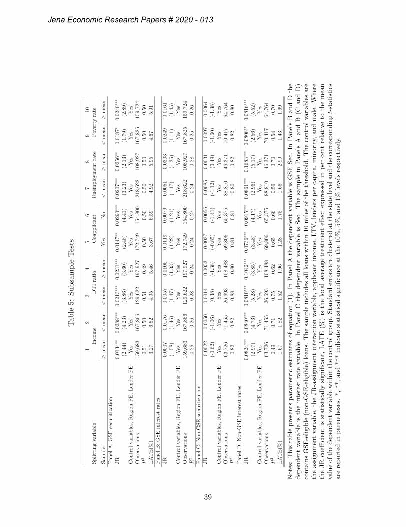
Tab
le5:
Subsa
mple
Tes
ts
12
34
56
78
910
Sp
litt
ing
vari
able
Inco
me
DT
Ira
tio
Coa
pp
lica
nt
Un
emp
loym
ent
rate
Pov
erty
rate
Sam
ple
≥m
ean
<m
ean
<m
ean≥
mea
nY
esN
o<
mea
n≥
mea
n<
mea
n≥
mea
nP
anel
A:
GS
Ese
curi
tiza
tion
JR
0.01
34∗∗
0.02
88∗∗
∗0.
0213
∗∗∗
0.02
31∗∗
∗0.
0147
∗∗0.
0290
∗∗∗
0.02
07∗∗
∗0.
0256
∗∗0.
0187
∗0.
0240
∗∗∗
(2.4
4)(4
.23)
(3.8
6)(3
.60)
(2.4
8)(4
.41)
(3.2
3)(2
.13)
(1.7
9)(2
.89)
Con
trol
vari
able
s,R
egio
nF
E,
Len
der
FE
Yes
Yes
Yes
Yes
Yes
Yes
Yes
Yes
Yes
Yes
Ob
serv
atio
ns
159,
683
167,
866
129,
622
197,
927
172,
749
154,
800
218,
622
108,
927
167,
825
159,
724
R2
0.51
0.50
0.51
0.49
0.50
0.50
0.50
0.50
0.50
0.50
LA
TE
(%)
3.27
6.52
4.95
5.46
3.67
6.59
4.92
5.95
4.67
5.91
Pan
elB
:G
SE
inte
rest
rate
sJR
0.00
070.
0176
0.00
570.
0105
0.01
190.
0079
0.00
510.
0303
0.02
490.
0161
(1.5
8)(1
.46)
(1.4
7)(1
.33)
(1.2
2)(1
.21)
(1.1
7)(1
.35)
(1.1
1)(1
.45)
Con
trol
vari
able
s,R
egio
nF
E,
Len
der
FE
Yes
Yes
Yes
Yes
Yes
Yes
Yes
Yes
Yes
Yes
Ob
serv
atio
ns
159,
683
167,
866
129,
622
197,
927
172,
749
154,
800
218,
622
108,
927
167,
825
159,
724
R2
0.26
0.26
0.28
0.24
0.24
0.27
0.24
0.28
0.25
0.26
Pan
elC
:N
on-G
SE
secu
riti
zati
onJR
-0.0
022
-0.0
050
0.00
14-0
.005
3-0
.003
7-0
.005
6-0
.008
50.
0031
-0.0
097
-0.0
064
(-0.
62)
(-1.
06)
(0.3
8)(-
1.38
)(-
0.85
)(-
1.41
)(-
1.12
)(0
.49)
(-1.
60)
(-1.
38)
Con
trol
vari
able
s,R
egio
nF
E,
Len
der
FE
Yes
Yes
Yes
Yes
Yes
Yes
Yes
Yes
Yes
Yes
Ob
serv
atio
ns
63,7
2671
,455
26,6
9310
8,48
869
,806
65,3
7588
,810
46,3
7170
,417
64,7
64R
20.
820.
820.
880.
800.
810.
810.
800.
820.
820.
80P
anel
D:
Non
-GS
Ein
tere
stra
tes
JR
0.08
24∗∗
∗0.
0840
∗∗∗
0.08
10∗∗
∗0.
1042
∗∗∗
0.07
36∗∗
∗0.
0915
∗∗∗
0.08
61∗∗
∗0.
1683
∗∗∗
0.08
08∗∗
0.08
16∗∗
∗
(2.9
7)(4
.73)
(5.2
8)(3
.85)
(3.4
8)(4
.17)
(2.9
6)(5
.17)
(2.5
6)(5
.52)
Con
trol
vari
able
s,R
egio
nF
E,
Len
der
FE
Yes
Yes
Yes
Yes
Yes
Yes
Yes
Yes
Yes
Yes
Ob
serv
atio
ns
63,7
2671
,455
26,6
9310
8,48
869
,806
65,3
7588
,810
46,3
7170
,417
64,7
64R
20.
490.
710.
750.
620.
650.
660.
590.
700.
540.
70L
AT
E(%
)1.
671.
821.
521.
961.
281.
751.
662.
991.
431.
69
Not
es:
Th
ista
ble
pre
sents
par
amet
ric
esti
mat
esof
equ
atio
n(1
).In
Pan
elA
the
dep
end
ent
vari
able
isG
SE
Sec
.In
Pan
els
Ban
dD
the
dep
end
ent
vari
ab
leis
the
inte
rest
rate
vari
able
.In
Pan
elC
the
dep
end
ent
vari
able
isS
ec.
Th
esa
mp
lein
Pan
els
Aan
dB
(Can
dD
)co
nta
ins
GS
E-e
ligi
ble
(non
-GS
E-e
ligi
ble
)lo
ans.
Th
esa
mp
lein
clu
des
all
loan
sw
ith
in10
mil
esof
the
thre
shol
d.
Th
eco
ntr
olva
riab
les
are
the
assi
gnm
ent
vari
able
,th
eJR
-ass
ign
men
tin
tera
ctio
nva
riab
le,
app
lica
nt
inco
me,
LT
V,
len
der
sp
erca
pit
a,m
inor
ity,
and
mal
e.W
her
eth
eJR
coeffi
cien
tis
stat
isti
call
ysi
gnifi
cant,
LA
TE
(%)
isth
elo
cal
aver
age
trea
tmen
teff
ect
exp
ress
edin
per
cent
rela
tive
toth
em
ean
valu
eof
the
dep
end
ent
vari
ab
lew
ith
inth
eco
ntr
olgr
oup
.S
tan
dar
der
rors
are
clu
ster
edat
the
stat
ele
vel
and
the
corr
esp
ond
ingt-
stat
isti
csar
ere
por
ted
inp
aren
thes
es.
*,**
,an
d**
*in
dic
ate
stat
isti
cal
sign
ifica
nce
atth
e10
%,
5%,
and
1%le
vels
resp
ecti
vely
.
39
Jena Economic Research Papers # 2020 - 013
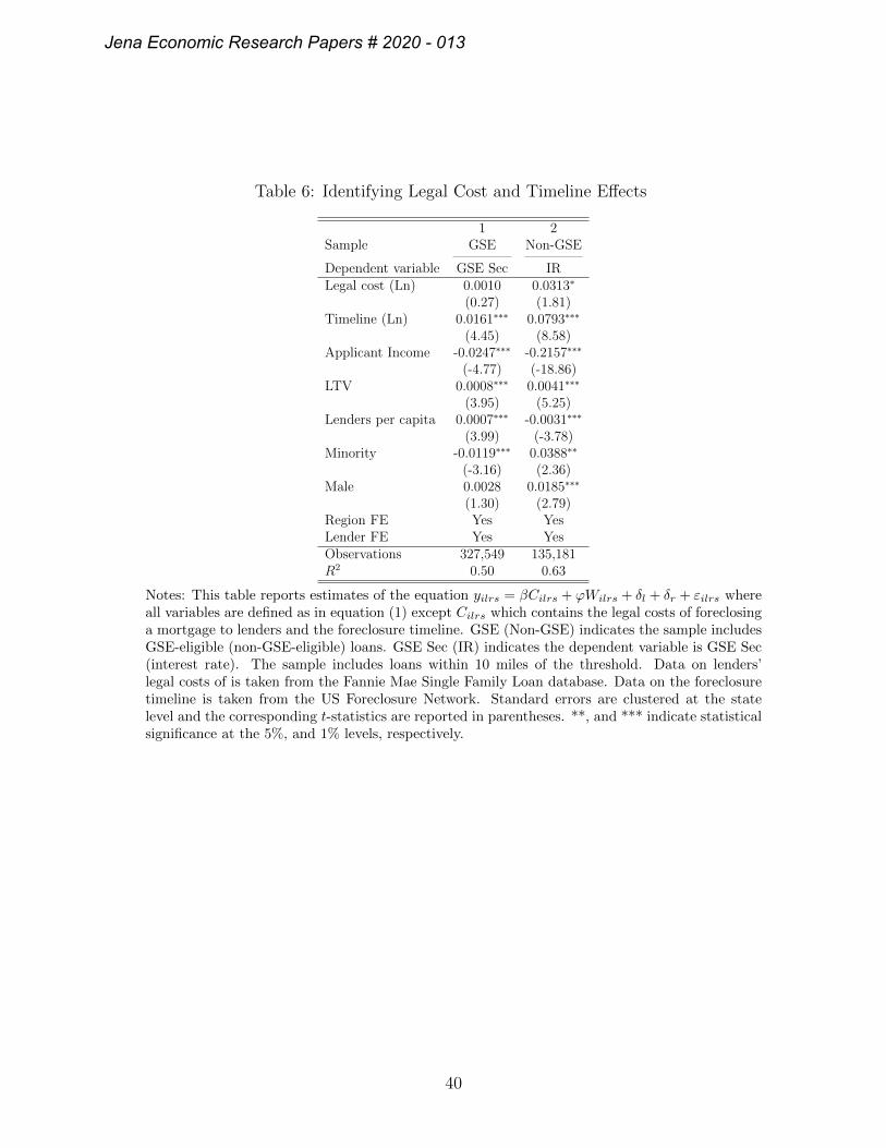
Table 6: Identifying Legal Cost and Timeline Effects
1 2Sample GSE Non-GSE
Dependent variable GSE Sec IRLegal cost (Ln) 0.0010 0.0313∗
(0.27) (1.81)Timeline (Ln) 0.0161∗∗∗ 0.0793∗∗∗
(4.45) (8.58)Applicant Income -0.0247∗∗∗ -0.2157∗∗∗
(-4.77) (-18.86)LTV 0.0008∗∗∗ 0.0041∗∗∗
(3.95) (5.25)Lenders per capita 0.0007∗∗∗ -0.0031∗∗∗
(3.99) (-3.78)Minority -0.0119∗∗∗ 0.0388∗∗
(-3.16) (2.36)Male 0.0028 0.0185∗∗∗
(1.30) (2.79)Region FE Yes YesLender FE Yes YesObservations 327,549 135,181R2 0.50 0.63
Notes: This table reports estimates of the equation yilrs = βCilrs + ϕWilrs + δl + δr + εilrs whereall variables are defined as in equation (1) except Cilrs which contains the legal costs of foreclosinga mortgage to lenders and the foreclosure timeline. GSE (Non-GSE) indicates the sample includesGSE-eligible (non-GSE-eligible) loans. GSE Sec (IR) indicates the dependent variable is GSE Sec(interest rate). The sample includes loans within 10 miles of the threshold. Data on lenders’legal costs of is taken from the Fannie Mae Single Family Loan database. Data on the foreclosuretimeline is taken from the US Foreclosure Network. Standard errors are clustered at the statelevel and the corresponding t-statistics are reported in parentheses. **, and *** indicate statisticalsignificance at the 5%, and 1% levels, respectively.
40
Jena Economic Research Papers # 2020 - 013
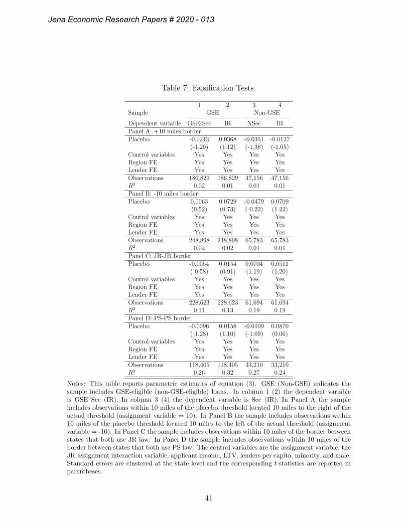
Table 7: Falsification Tests
1 2 3 4Sample GSE Non-GSE
Dependent variable GSE Sec IR NSec IRPanel A: +10 miles borderPlacebo -0.0213 0.0368 -0.0351 -0.0127
(-1.29) (1.12) (-1.38) (-1.05)Control variables Yes Yes Yes YesRegion FE Yes Yes Yes YesLender FE Yes Yes Yes YesObservations 186,829 186,829 47,156 47,156R2 0.02 0.01 0.01 0.01Panel B: -10 miles borderPlacebo 0.0063 0.0729 -0.0479 0.0709
(0.52) (0.73) (-0.22) (1.22)Control variables Yes Yes Yes YesRegion FE Yes Yes Yes YesLender FE Yes Yes Yes YesObservations 248,898 248,898 65,783 65,783R2 0.02 0.02 0.01 0.01Panel C: JR-JR borderPlacebo -0.0054 0.0154 0.0704 0.0511
(-0.58) (0.91) (1.19) (1.20)Control variables Yes Yes Yes YesRegion FE Yes Yes Yes YesLender FE Yes Yes Yes YesObservations 228,623 228,623 61,694 61,694R2 0.11 0.13 0.19 0.19Panel D: PS-PS borderPlacebo -0.0096 0.0158 -0.0109 0.0870
(-1.28) (1.10) (-1.09) (0.06)Control variables Yes Yes Yes YesRegion FE Yes Yes Yes YesLender FE Yes Yes Yes YesObservations 118,405 118,405 33,210 33,210R2 0.26 0.32 0.27 0.24
Notes: This table reports parametric estimates of equation (3). GSE (Non-GSE) indicates thesample includes GSE-eligible (non-GSE-eligible) loans. In column 1 (2) the dependent variableis GSE Sec (IR). In column 3 (4) the dependent variable is Sec (IR). In Panel A the sampleincludes observations within 10 miles of the placebo threshold located 10 miles to the right of theactual threshold (assignment variable = 10). In Panel B the sample includes observations within10 miles of the placebo threshold located 10 miles to the left of the actual threshold (assignmentvariable = -10). In Panel C the sample includes observations within 10 miles of the border betweenstates that both use JR law. In Panel D the sample includes observations within 10 miles of theborder between states that both use PS law. The control variables are the assignment variable, theJR-assignment interaction variable, applicant income, LTV, lenders per capita, minority, and male.Standard errors are clustered at the state level and the corresponding t-statistics are reported inparentheses.
41
Jena Economic Research Papers # 2020 - 013
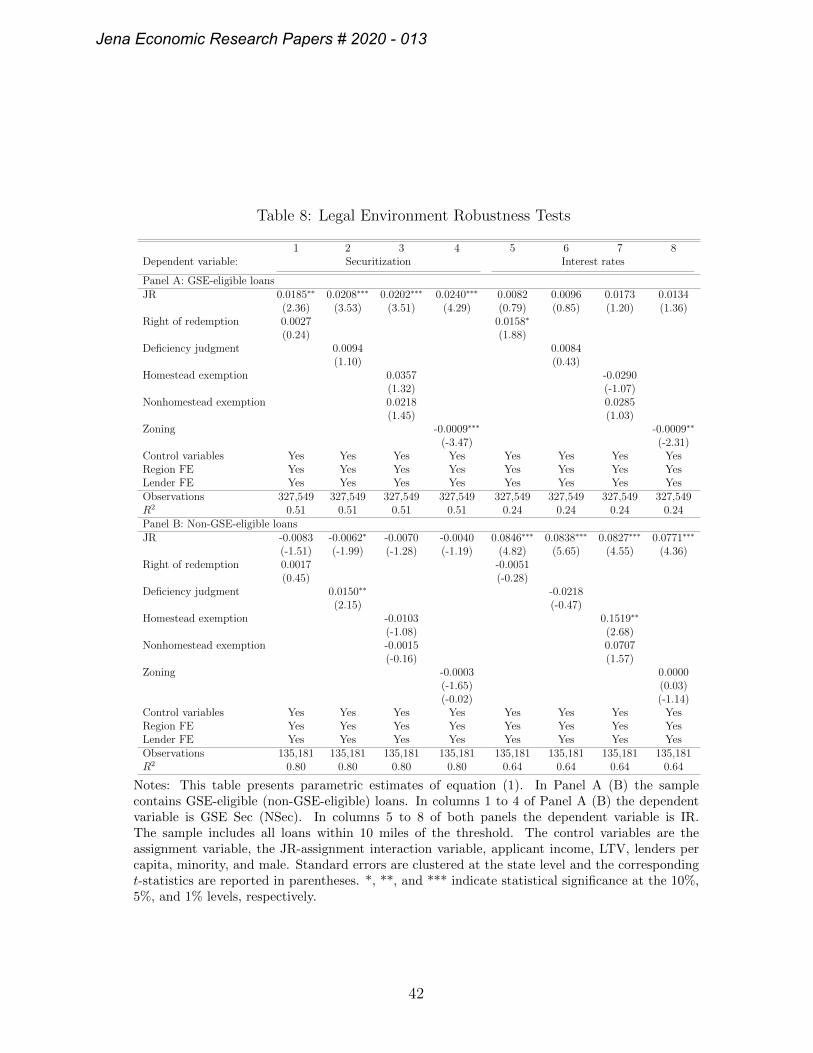
Table 8: Legal Environment Robustness Tests
1 2 3 4 5 6 7 8Dependent variable: Securitization Interest rates
Panel A: GSE-eligible loansJR 0.0185∗∗ 0.0208∗∗∗ 0.0202∗∗∗ 0.0240∗∗∗ 0.0082 0.0096 0.0173 0.0134
(2.36) (3.53) (3.51) (4.29) (0.79) (0.85) (1.20) (1.36)Right of redemption 0.0027 0.0158∗
(0.24) (1.88)Deficiency judgment 0.0094 0.0084
(1.10) (0.43)Homestead exemption 0.0357 -0.0290
(1.32) (-1.07)Nonhomestead exemption 0.0218 0.0285
(1.45) (1.03)Zoning -0.0009∗∗∗ -0.0009∗∗
(-3.47) (-2.31)Control variables Yes Yes Yes Yes Yes Yes Yes YesRegion FE Yes Yes Yes Yes Yes Yes Yes YesLender FE Yes Yes Yes Yes Yes Yes Yes YesObservations 327,549 327,549 327,549 327,549 327,549 327,549 327,549 327,549R2 0.51 0.51 0.51 0.51 0.24 0.24 0.24 0.24Panel B: Non-GSE-eligible loansJR -0.0083 -0.0062∗ -0.0070 -0.0040 0.0846∗∗∗ 0.0838∗∗∗ 0.0827∗∗∗ 0.0771∗∗∗
(-1.51) (-1.99) (-1.28) (-1.19) (4.82) (5.65) (4.55) (4.36)Right of redemption 0.0017 -0.0051
(0.45) (-0.28)Deficiency judgment 0.0150∗∗ -0.0218
(2.15) (-0.47)Homestead exemption -0.0103 0.1519∗∗
(-1.08) (2.68)Nonhomestead exemption -0.0015 0.0707
(-0.16) (1.57)Zoning -0.0003 0.0000
(-1.65) (0.03)(-0.02) (-1.14)
Control variables Yes Yes Yes Yes Yes Yes Yes YesRegion FE Yes Yes Yes Yes Yes Yes Yes YesLender FE Yes Yes Yes Yes Yes Yes Yes YesObservations 135,181 135,181 135,181 135,181 135,181 135,181 135,181 135,181R2 0.80 0.80 0.80 0.80 0.64 0.64 0.64 0.64
Notes: This table presents parametric estimates of equation (1). In Panel A (B) the samplecontains GSE-eligible (non-GSE-eligible) loans. In columns 1 to 4 of Panel A (B) the dependentvariable is GSE Sec (NSec). In columns 5 to 8 of both panels the dependent variable is IR.The sample includes all loans within 10 miles of the threshold. The control variables are theassignment variable, the JR-assignment interaction variable, applicant income, LTV, lenders percapita, minority, and male. Standard errors are clustered at the state level and the correspondingt-statistics are reported in parentheses. *, **, and *** indicate statistical significance at the 10%,5%, and 1% levels, respectively.
42
Jena Economic Research Papers # 2020 - 013
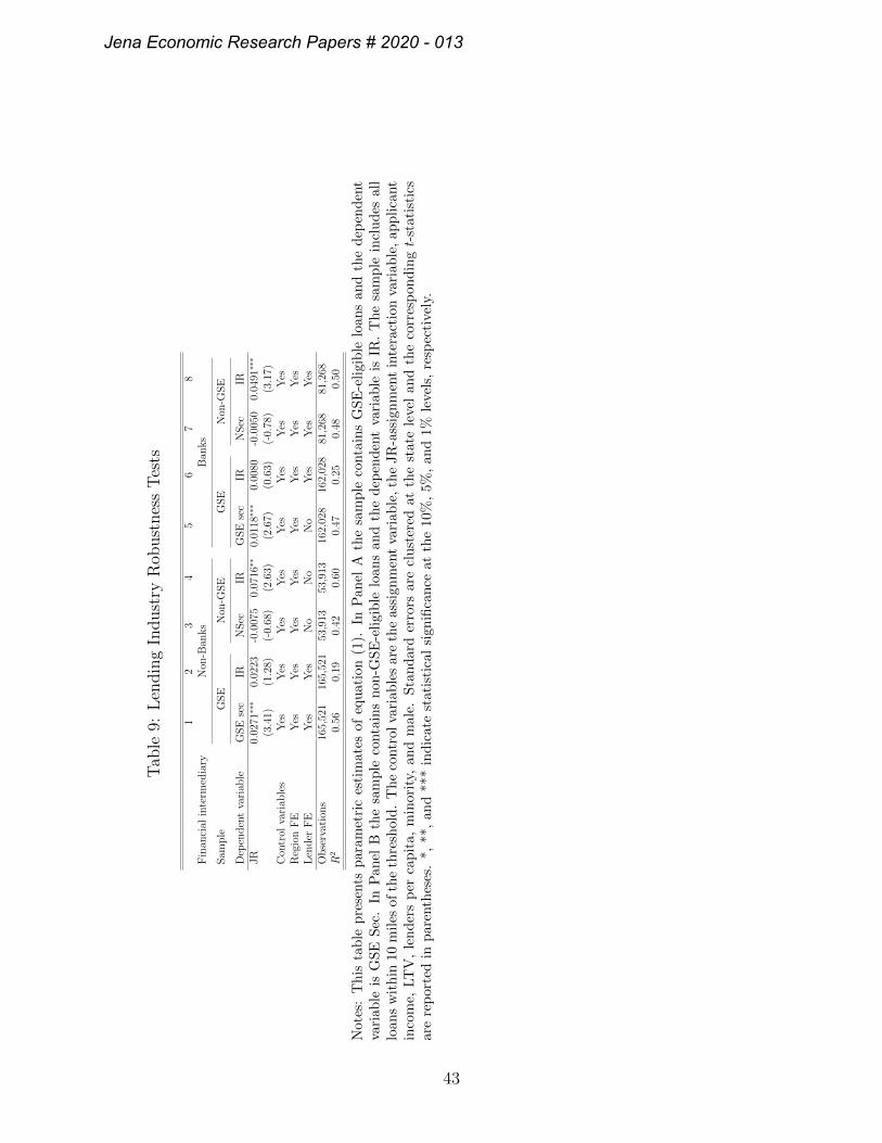
Tab
le9:
Len
din
gIn
dust
ryR
obust
nes
sT
ests
12
34
56
78
Fin
anci
alin
term
edia
ryN
on-B
anks
Ban
ks
Sam
ple
GS
EN
on-G
SE
GS
EN
on-G
SE
Dep
end
ent
vari
able
GS
Ese
cIR
NS
ecIR
GS
Ese
cIR
NS
ecIR
JR
0.02
71∗∗
∗0.
0223
-0.0
075
0.07
16∗∗
0.01
18∗∗
∗0.
0080
-0.0
050
0.04
91∗∗
∗
(3.4
1)(1
.28)
(-0.
68)
(2.6
3)(2
.67)
(0.6
3)(-
0.78
)(3
.17)
Con
trol
vari
able
sY
esY
esY
esY
esY
esY
esY
esY
esR
egio
nF
EY
esY
esY
esY
esY
esY
esY
esY
esL
end
erF
EY
esY
esN
oN
oN
oY
esY
esY
esO
bse
rvat
ion
s16
5,52
116
5,52
153
,913
53,9
1316
2,02
816
2,02
881
,268
81,2
68R
20.
560.
190.
420.
600.
470.
250.
480.
50
Not
es:
Th
ista
ble
pre
sents
par
amet
ric
esti
mat
esof
equ
atio
n(1
).In
Pan
elA
the
sam
ple
conta
ins
GS
E-e
ligi
ble
loan
san
dth
ed
epen
den
tva
riab
leis
GS
ES
ec.
InP
anel
Bth
esa
mp
leco
nta
ins
non
-GS
E-e
ligi
ble
loan
san
dth
ed
epen
den
tva
riab
leis
IR.
The
sam
ple
incl
ud
esal
llo
ans
wit
hin
10m
iles
ofth
eth
resh
old
.T
he
contr
olva
riab
les
are
the
assi
gnm
ent
vari
able
,th
eJR
-ass
ign
men
tin
tera
ctio
nva
riab
le,
app
lica
nt
inco
me,
LT
V,
len
der
sp
erca
pit
a,m
inori
ty,
an
dm
ale.
Sta
nd
ard
erro
rsar
ecl
ust
ered
atth
est
ate
level
and
the
corr
esp
ond
ingt-
stat
isti
csar
ere
por
ted
inp
aren
thes
es.
*,
**,
and
***
ind
icat
est
atis
tica
lsi
gnifi
can
ceat
the
10%
,5%
,an
d1%
leve
ls,
resp
ecti
vely
.
43
Jena Economic Research Papers # 2020 - 013
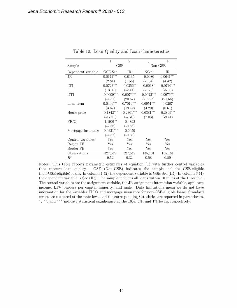
Table 10: Loan Quality and Loan characteristics
1 2 3 4Sample GSE Non-GSE
Dependent variable GSE Sec IR NSec IRJR 0.0172∗∗∗ 0.0135 -0.0080 0.0641∗∗∗
(2.81) (1.56) (-1.54) (4.42)LTI 0.0723∗∗∗ -0.0356∗∗ -0.0068∗ -0.0740∗∗∗
(13.09) (-2.41) (-1.78) (-5.03)DTI -0.0009∗∗∗ 0.0076∗∗∗ -0.0022∗∗∗ 0.0076∗∗∗
(-4.31) (20.67) (-15.93) (21.66)Loan term 0.0496∗∗∗ 0.7019∗∗∗ 0.0951∗∗∗ 0.0267
(3.67) (19.42) (4.20) (0.61)House price -0.1842∗∗∗ -0.2301∗∗∗ 0.0381∗∗∗ -0.2899∗∗∗
(-17.21) (-7.70) (7.03) (-9.41)FICO -1.1901∗∗ -0.4892
(-2.68) (-0.63)Mortgage Insurance -0.0321∗∗∗ -0.0050
(-4.67) (-0.58)Control varaibles Yes Yes Yes YesRegion FE Yes Yes Yes YesBorder FE Yes Yes Yes YesObservations 327,549 327,549 135,181 135,181R2 0.52 0.32 0.58 0.59
Notes: This table reports parametric estimates of equation (1) with further control variablesthat capture loan quality. GSE (Non-GSE) indicates the sample includes GSE-eligible(non-GSE-eligible) loans. In column 1 (2) the dependent variable is GSE Sec (IR). In column 3 (4)the dependent variable is Sec (IR). The sample includes all loans within 10 miles of the threshold.The control variables are the assignment variable, the JR-assignment interaction variable, applicantincome, LTV, lenders per capita, minority, and male. Data limitations mean we do not haveinformation for the variables FICO and mortgage insurance for non-GSE-eligible loans. Standarderrors are clustered at the state level and the corresponding t-statistics are reported in parentheses.*, **, and *** indicate statistical significance at the 10%, 5%, and 1% levels, respectively.
44
Jena Economic Research Papers # 2020 - 013
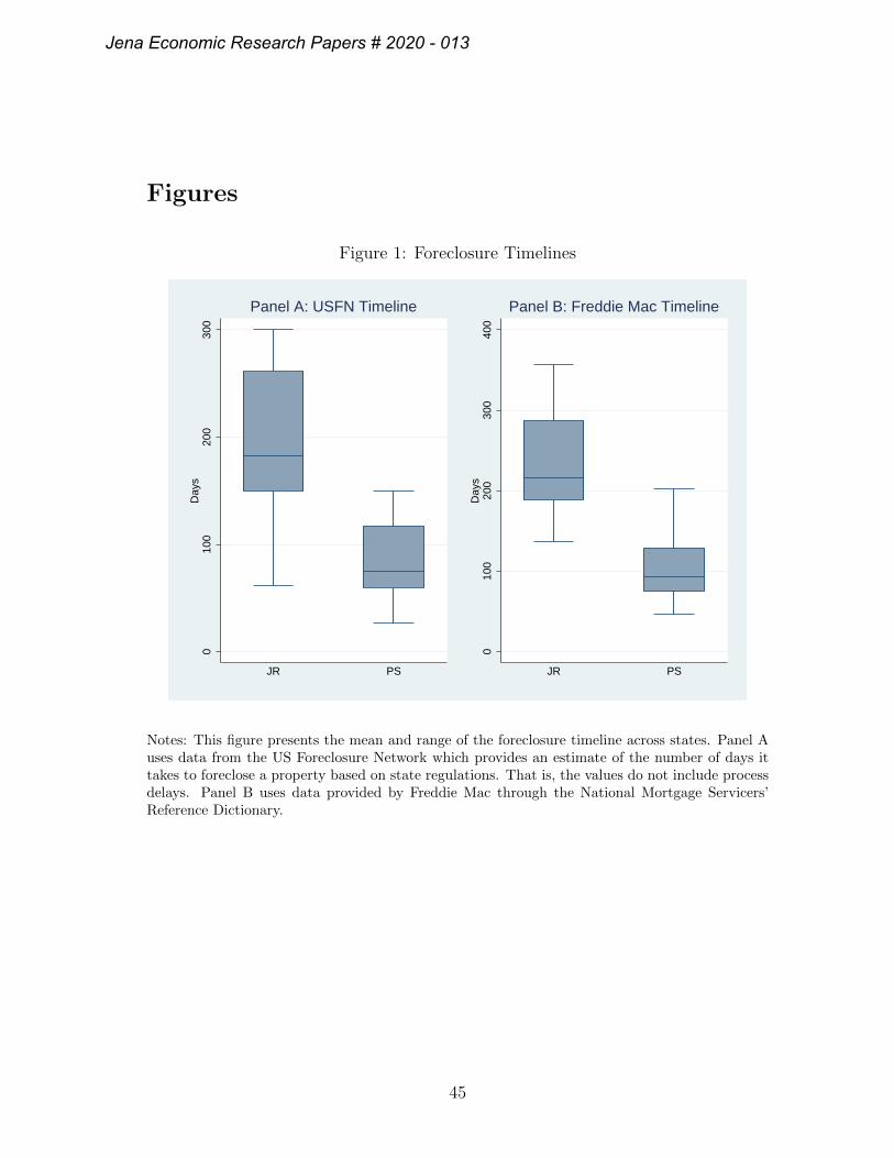
Figures
Figure 1: Foreclosure Timelines
010
020
030
0D
ays
JR PS
Panel A: USFN Timeline
010
020
030
040
0D
ays
JR PS
Panel B: Freddie Mac Timeline
Notes: This figure presents the mean and range of the foreclosure timeline across states. Panel Auses data from the US Foreclosure Network which provides an estimate of the number of days ittakes to foreclose a property based on state regulations. That is, the values do not include processdelays. Panel B uses data provided by Freddie Mac through the National Mortgage Servicers’Reference Dictionary.
45
Jena Economic Research Papers # 2020 - 013
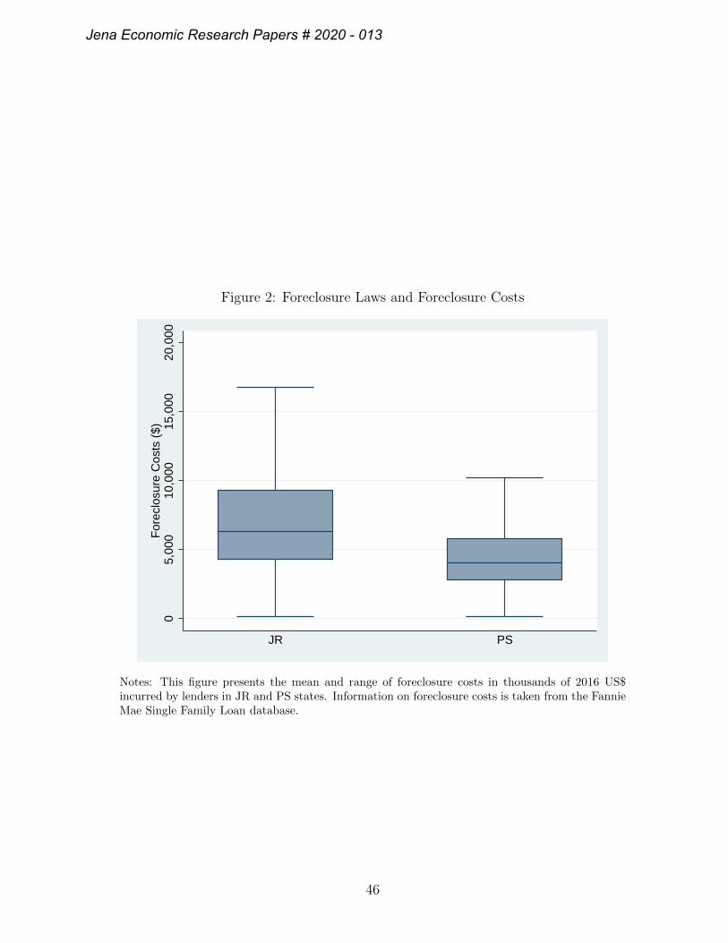
Figure 2: Foreclosure Laws and Foreclosure Costs
05,
000
10,0
0015
,000
20,0
00F
orec
losu
re C
osts
($)
JR PS
Notes: This figure presents the mean and range of foreclosure costs in thousands of 2016 US$incurred by lenders in JR and PS states. Information on foreclosure costs is taken from the FannieMae Single Family Loan database.
46
Jena Economic Research Papers # 2020 - 013
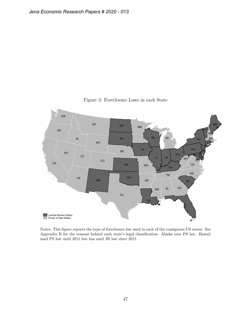
Figure 3: Foreclosure Laws in each State
AL
AZAR
CACO
CT
DEDC
FL
GA
ID
IL IN
IA
KSKY
LA
ME
MD
MAMI
MN
MS
MO
MT
NENV
NH
NJ
NM
NY
NC
ND
OH
OK
OR
PA
RI
SC
SD
TN
TX
UT
VT
VA
WA
WV
WI
WY
Judicial Review StatesPower of Sale States
Notes: This figure reports the type of foreclosure law used in each of the contiguous US states. SeeAppendix B for the reasons behind each state’s legal classification. Alaska uses PS law. Hawaiiused PS law until 2011 but has used JR law since 2011.
47
Jena Economic Research Papers # 2020 - 013
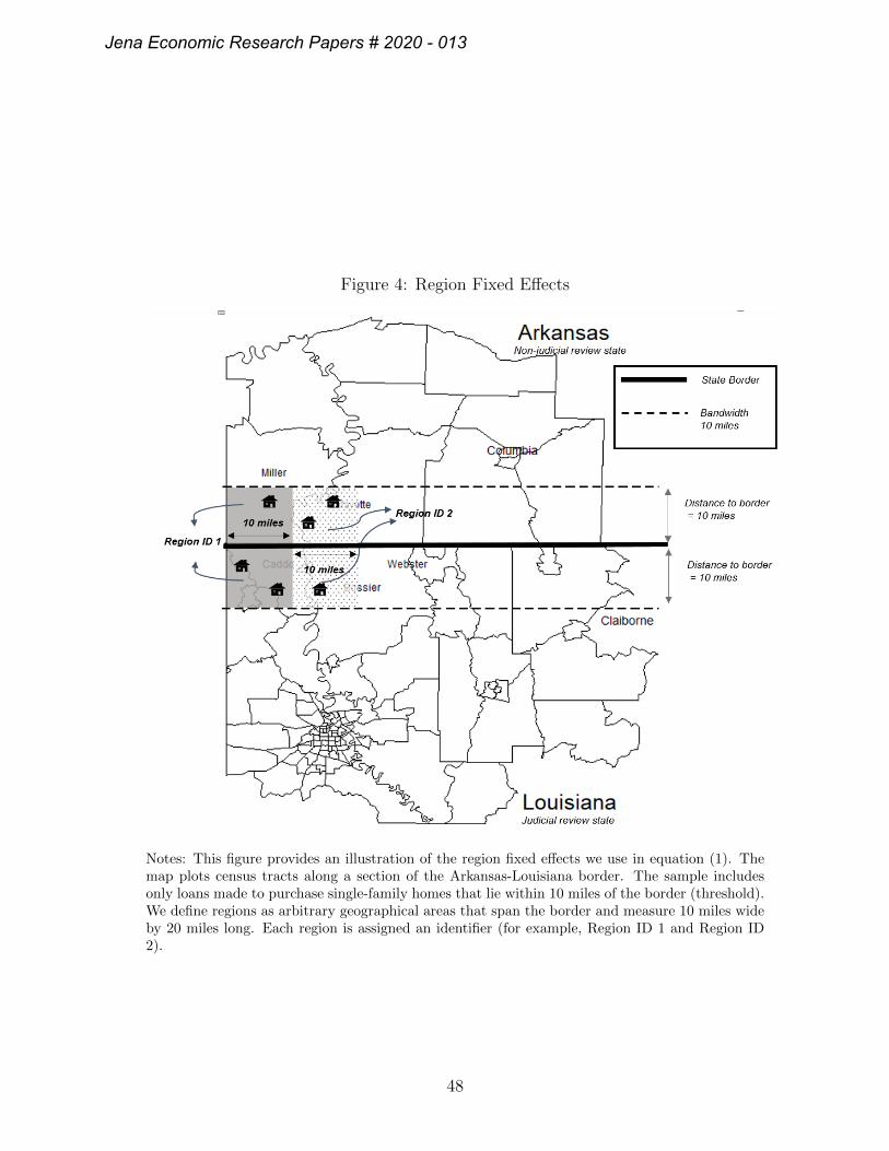
Figure 4: Region Fixed Effects
Notes: This figure provides an illustration of the region fixed effects we use in equation (1). Themap plots census tracts along a section of the Arkansas-Louisiana border. The sample includesonly loans made to purchase single-family homes that lie within 10 miles of the border (threshold).We define regions as arbitrary geographical areas that span the border and measure 10 miles wideby 20 miles long. Each region is assigned an identifier (for example, Region ID 1 and Region ID2).
48
Jena Economic Research Papers # 2020 - 013
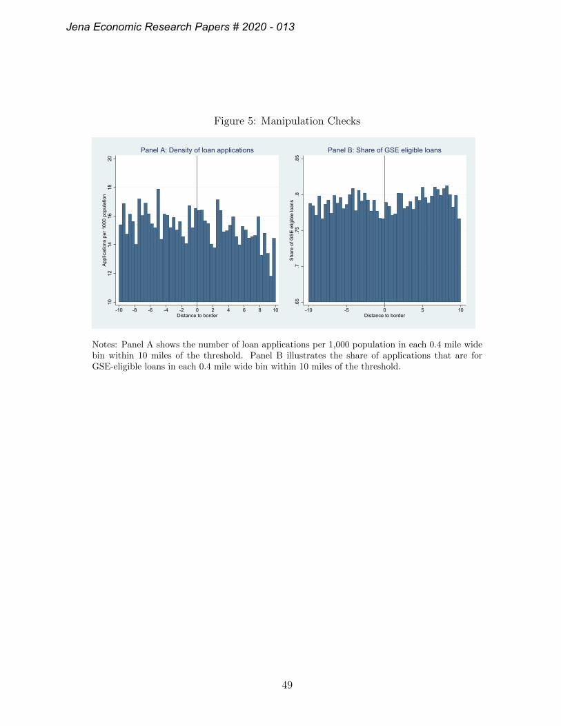
Figure 5: Manipulation Checks10
1214
1618
20Ap
plic
atio
ns p
er 1
000
popu
latio
n
-10 -8 -6 -4 -2 0 2 4 6 8 10Distance to border
Panel A: Density of loan applications
.65
.7.7
5.8
.85
Shar
e of
GSE
elig
ible
loan
s
-10 -5 0 5 10Distance to border
Panel B: Share of GSE eligible loans
Notes: Panel A shows the number of loan applications per 1,000 population in each 0.4 mile widebin within 10 miles of the threshold. Panel B illustrates the share of applications that are forGSE-eligible loans in each 0.4 mile wide bin within 10 miles of the threshold.
49
Jena Economic Research Papers # 2020 - 013
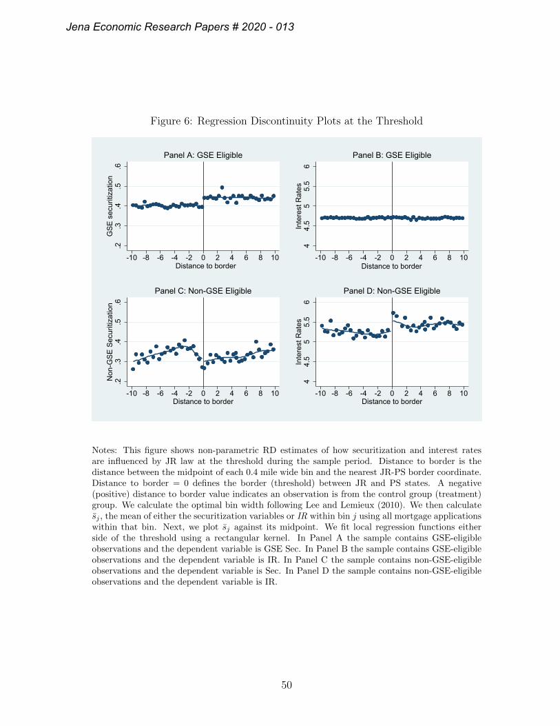
Figure 6: Regression Discontinuity Plots at the Threshold.2
.3.4
.5.6
GSE
sec
uriti
zatio
n
-10 -8 -6 -4 -2 0 2 4 6 8 10Distance to border
Panel A: GSE Eligible
44.
55
5.5
6In
tere
st R
ates
-10 -8 -6 -4 -2 0 2 4 6 8 10Distance to border
Panel B: GSE Eligible
.2.3
.4.5
.6N
on-G
SE S
ecur
itiza
tion
-10 -8 -6 -4 -2 0 2 4 6 8 10Distance to border
Panel C: Non-GSE Eligible
44.
55
5.5
6In
tere
st R
ates
-10 -8 -6 -4 -2 0 2 4 6 8 10Distance to border
Panel D: Non-GSE Eligible
Notes: This figure shows non-parametric RD estimates of how securitization and interest ratesare influenced by JR law at the threshold during the sample period. Distance to border is thedistance between the midpoint of each 0.4 mile wide bin and the nearest JR-PS border coordinate.Distance to border = 0 defines the border (threshold) between JR and PS states. A negative(positive) distance to border value indicates an observation is from the control group (treatment)group. We calculate the optimal bin width following Lee and Lemieux (2010). We then calculatesj , the mean of either the securitization variables or IR within bin j using all mortgage applicationswithin that bin. Next, we plot sj against its midpoint. We fit local regression functions eitherside of the threshold using a rectangular kernel. In Panel A the sample contains GSE-eligibleobservations and the dependent variable is GSE Sec. In Panel B the sample contains GSE-eligibleobservations and the dependent variable is IR. In Panel C the sample contains non-GSE-eligibleobservations and the dependent variable is Sec. In Panel D the sample contains non-GSE-eligibleobservations and the dependent variable is IR.
50
Jena Economic Research Papers # 2020 - 013
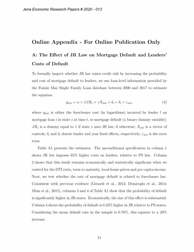
Online Appendix - For Online Publication Only
A: The Effect of JR Law on Mortgage Default and Lenders’
Costs of Default
To formally inspect whether JR law raises credit risk by increasing the probability
and cost of mortgage default to lenders, we use loan-level information provided by
the Fannie Mae Single Family Loan database between 2000 and 2017 to estimate
the equation
yilst = α + βJRs + γXilst + δl + δt + εilst, (4)
where yilst is either the foreclosure cost (in logarithms) incurred by lender l on
mortgage loan i in state s at time t, or mortgage default (a binary dummy variable);
JRs is a dummy equal to 1 if state s uses JR law, 0 otherwise; Xilst is a vector of
controls; δl and δt denote lender and year fixed effects, respectively; εilst is the error
term.
Table A1 presents the estimates. The unconditional specification in column 1
shows JR law imposes 65% higher costs on lenders, relative to PS law. Column
2 shows that this result remains economically and statistically significant when we
control for the DTI ratio, term to maturity, local house prices and per capita income.
Next, we test whether the rate of mortgage default is related to foreclosure law.
Consistent with previous evidence (Gerardi et al., 2013; Demiroglu et al., 2014;
Mian et al., 2015), columns 3 and 4 of Table A1 show that the probability of default
is significantly higher in JR states. Economically, the size of this effect is substantial.
Column 4 shows the probability of default is 0.23% higher in JR relative to PS states.
Considering the mean default rate in the sample is 0.78%, this equates to a 29%
increase.
51
Jena Economic Research Papers # 2020 - 013
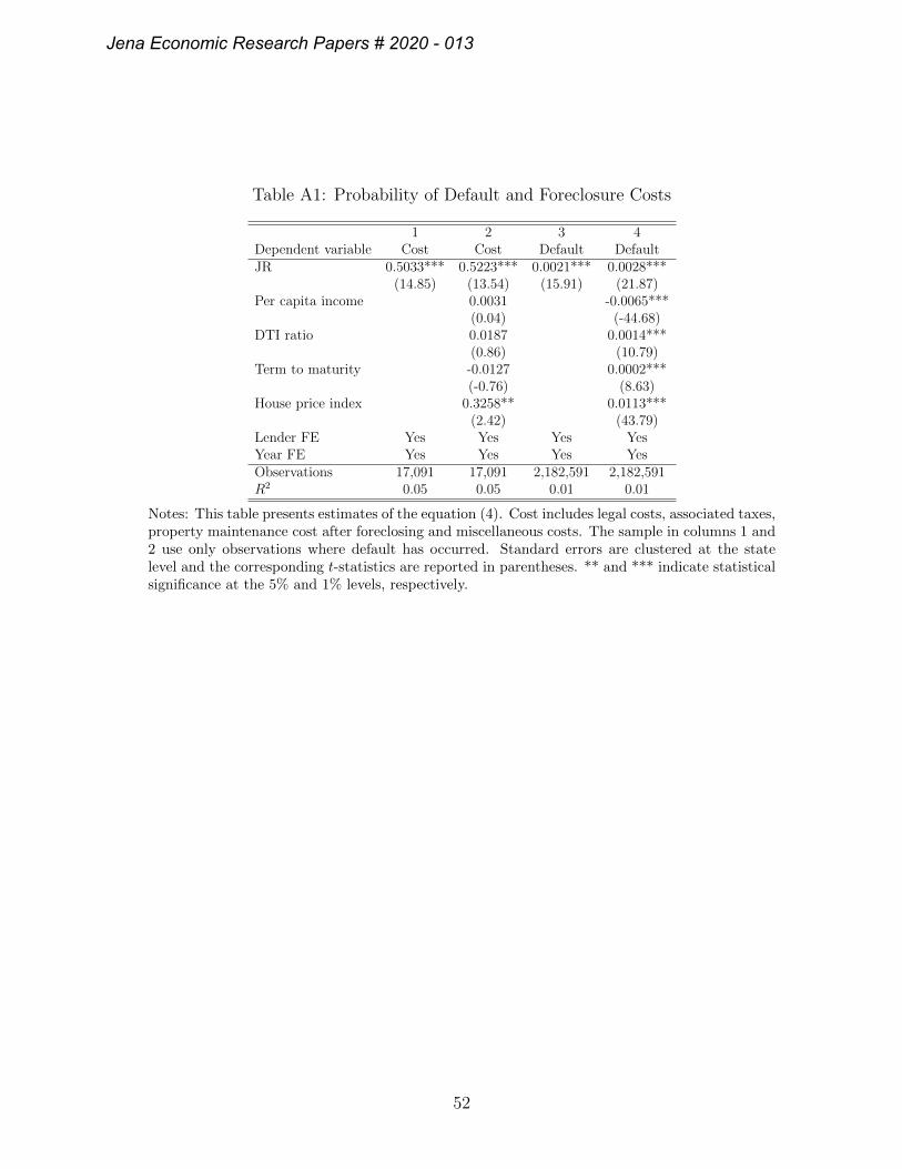
Table A1: Probability of Default and Foreclosure Costs
1 2 3 4Dependent variable Cost Cost Default DefaultJR 0.5033*** 0.5223*** 0.0021*** 0.0028***
(14.85) (13.54) (15.91) (21.87)Per capita income 0.0031 -0.0065***
(0.04) (-44.68)DTI ratio 0.0187 0.0014***
(0.86) (10.79)Term to maturity -0.0127 0.0002***
(-0.76) (8.63)House price index 0.3258** 0.0113***
(2.42) (43.79)Lender FE Yes Yes Yes YesYear FE Yes Yes Yes YesObservations 17,091 17,091 2,182,591 2,182,591R2 0.05 0.05 0.01 0.01
Notes: This table presents estimates of the equation (4). Cost includes legal costs, associated taxes,property maintenance cost after foreclosing and miscellaneous costs. The sample in columns 1 and2 use only observations where default has occurred. Standard errors are clustered at the statelevel and the corresponding t-statistics are reported in parentheses. ** and *** indicate statisticalsignificance at the 5% and 1% levels, respectively.
52
Jena Economic Research Papers # 2020 - 013
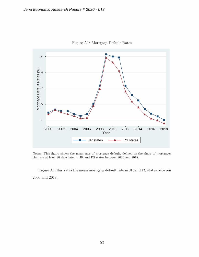
Figure A1: Mortgage Default Rates1
23
45
Mor
tgag
e D
efau
lt R
ates
(%)
2000 2002 2004 2006 2008 2010 2012 2014 2016 2018Year
JR states PS states
Notes: This figure shows the mean rate of mortgage default, defined as the share of mortgagesthat are at least 90 days late, in JR and PS states between 2000 and 2018.
Figure A1 illustrates the mean mortgage default rate in JR and PS states between
2000 and 2018.
53
Jena Economic Research Papers # 2020 - 013
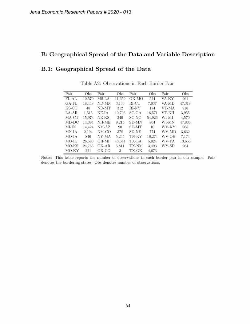
B: Geographical Spread of the Data and Variable Description
B.1: Geographical Spread of the Data
Table A2: Observations in Each Border Pair
Pair Obs Pair Obs Pair Obs Pair ObsFL-AL 10,570 MS-LA 11,659 OK-MO 524 VA-KY 961GA-FL 18,448 ND-MN 3,136 RI-CT 7,037 VA-MD 47,318KS-CO 48 ND-MT 312 RI-NY 174 VT-MA 918LA-AR 1,515 NE-IA 10,706 SC-GA 16,571 VT-NH 3,955MA-CT 15,973 NE-KS 340 SC-NC 54,926 WI-MI 4,570MD-DC 14,394 NH-ME 9,215 SD-MN 804 WI-MN 47,833MI-IN 14,424 NM-AZ 90 SD-MT 10 WV-KY 965MN-IA 2,194 NM-CO 378 SD-NE 774 WV-MD 3,632MO-IA 846 NY-MA 5,245 TN-KY 16,274 WV-OH 7,174MO-IL 26,593 OH-MI 43,644 TX-LA 5,024 WV-PA 13,653MO-KS 24,765 OK-AR 5,811 TX-NM 3,493 WY-SD 964MO-KY 221 OK-CO 3 TX-OK 4,673
Notes: This table reports the number of observations in each border pair in our sample. Pairdenotes the bordering states. Obs denotes number of observations.
54
Jena Economic Research Papers # 2020 - 013
B.2: Variable Definitions
Variable Definitions
Sec (GSE-eligible): a dummy variable equal to 1 if a GSE-eligible loan is securitized,
0 otherwise.
GSE Sec (GSE-eligible): a dummy variable equal to 1 if a GSE-eligible loan is
securitized through sale to Fannie Mae or Freddie Mac, 0 otherwise.
Private Sec (GSE-eligible): a dummy variable equal to 1 if a GSE-eligible loan is
securitized through sale to a private securitizer, 0 otherwise.
NSec (Non-GSE-eligible): a dummy variable equal to 1 if a non-GSE-eligible loan
is securitized, 0 otherwise.
IR (GSE-eligible): the interest rate on a GSE-eligible loan.
IR (Non-GSE-eligible): the interest rate on a non-GSE-eligible loan.
JR: a dummy variable equal to 1 if loan i is on a property located in a Judicial
Review state, 0 if the property is located in a Power of Sale state.
Assignment : the distance in miles between the midpoint of the census tract that
loan i is located and the nearest JR-PS border coordinate.
GSE-eligible: a dummy variable equal to 1 if loan i is eligible for sale to Fannie Mae
or Freddie Mac, 0 otherwise.
Loan amount : the origination amount on loan i.
Applicant income: the annual income of the borrower on loan i.
LTV : the loan-to-income ratio on loan i.
Male: a dummy variable equal to 1 if the applicant on loan i is male, 0 otherwise.
Minority : a dummy variable equal to 1 if the applicant on loan i is from an ethnic
minority, 0 otherwise.
Lenders per capita: the number of lenders per 1,000 population in the census tract
where loan i is located.
55
Jena Economic Research Papers # 2020 - 013
LTI ratio: the ratio of the loan amount to applicant income on loan i.
Co-applicant : a dummy variable equal to 1 if there is a coapplicant on loan i, 0
otherwise.
Applicants per capita: the number of mortgage applications per 1,000 population in
the census tract where loan i is located.
House prices : the FHFA house price index in the census tract where loan i is located.
Renter occupied housing : the ratio of rented properties to total properties in the
county where loan i is located.
Arrangement fee: the mean of the ratio of the arrangement fee to loan amount in
the county where loan i is located.
Loan term: term to maturity (in months) on loan i.
Mortgage insurance: the share of GSE-eligible loans with mortgage insurance in the
county where loan i is located.
DTI : the debt-to-income ratio of loan i.
FICO : the mean FICO score of mortgages in the county where loan i is located.
Right of redemption: a dummy variable equal to 1 if loan i is located in a state that
permits right of redemption within 12 months of foreclosure, 0 otherwise.
Deficiency judgment : a dummy variable equal to 1 if loan i is located in a state that
permits deficiency judgment, 0 otherwise.
Homestead exemption: the maximum value of property that is exempt in bankruptcy
in the state where loan i is located is located.
Nonhomestead exemption: the the sum of automobile, other property, and wildcard
exemptions that is exempt in bankruptcy in the state where loan i is located.
Zoning index : an index measuring the intensity of restrictions on building single-unit
homes in the state loan i is located.
Legal cost : the mean cost to lenders of foreclosing a loan in the state loan i is located.
Timeline: the mean duration of the foreclosure process (excluding process delays)
56
Jena Economic Research Papers # 2020 - 013
in the state loan i is located.
Renegotiation rate: the ratio of delinquent borrowers that successfully renegotiate
terms with the mortgage servicer to total delinquent loans in the county loan i is
located.
Refinancing rate: the ratio of refinancing loan applications to total mortgage applica-
tions in the census tract where loan i is located.
State corporate tax rate: the top marginal state corporate income tax rate in the
state loan i is located.
State personal tax rate: the top marginal state personal income tax rate in the state
loan i is located.
Auto delinquency rate: the ratio of auto loans that are at least 90 days delinquent
to total auto loans in the county loan i is located.
Credit card delinquency rate: the ratio of credit card loans that are at least 90 days
delinquent to total credit card loans in the county loan i is located.
Adjustable rate loan: the ratio of adjustable rate loans to total mortgage loans in
the county loan i is located.
HHI : a Herfindahl-Hirschman index of lenders’ market shares in the county where
loan i. Market share is the ratio of the total value of mortgage loans originated in
county c by lender l relative to the total value of mortgage loans originated by all
institutions in county c.
Nonbank : a dummy variable equal to 1 if loan i is originated by a non-depository
institution.
Bank size: total assets of lender l.
Z-score: calculated using the formula Zl = (ROAl +ETAl)/ROASDl where ROAl,
ETAl, and ROASDl are return on assets, the ratio of equity to total assets, and
the standard deviation of returns on assets over the 4 quarters of 2018 for bank l,
respectively.
57
Jena Economic Research Papers # 2020 - 013
Capital ratio: the ratio of equity capital to total assets for lender l.
Non-bank : a dummy variable equal to 1 if loan i is originated by a non-deposit
taking institution.
NII ratio: the ratio of net interest income to total assets for lender l.
Cost of deposits : the ratio of deposit interest expenses to deposit liabilities for lender
l.
Out of state: a dummy variable equal to 1 if loan i is located in a state outside
lender l’s headquarter state.
Unemployment rate: the unemployment rate in the county loan i is located.
Per capita income: the level of income per capita in the county loan i is located.
Urbanization: a dummy variable equal to 1 if loan i is located in urban areas.
Poverty rate: the ratio of the population living below the poverty line to total
population in the county loan i is located.
Black population: the ratio of the population who are black to total population in
the county loan i is located.
Hispanic population: the ratio of the population who are Hispanic to total population
in the county loan i is located.
Violent crime rate: the number of violent crimes per 1,000 population in the county
loan i is located.
Degree: the ratio of the number of people with at least a College degree eduation
to total population in the county loan i is located.
Net migration: net migration (immigration minus emigration) per 1,000 population
into county c between 2013 and 2017.
58
Jena Economic Research Papers # 2020 - 013
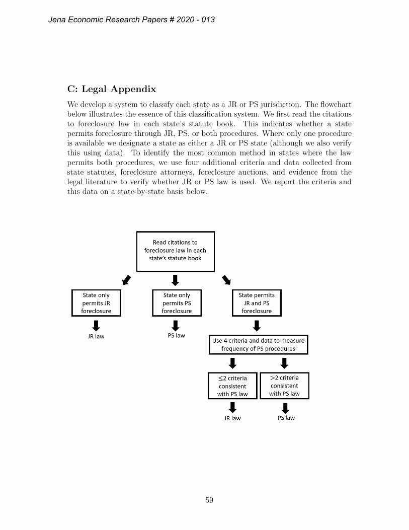
C: Legal Appendix
We develop a system to classify each state as a JR or PS jurisdiction. The flowchartbelow illustrates the essence of this classification system. We first read the citationsto foreclosure law in each state’s statute book. This indicates whether a statepermits foreclosure through JR, PS, or both procedures. Where only one procedureis available we designate a state as either a JR or PS state (although we also verifythis using data). To identify the most common method in states where the lawpermits both procedures, we use four additional criteria and data collected fromstate statutes, foreclosure attorneys, foreclosure auctions, and evidence from thelegal literature to verify whether JR or PS law is used. We report the criteria andthis data on a state-by-state basis below.
59
Jena Economic Research Papers # 2020 - 013
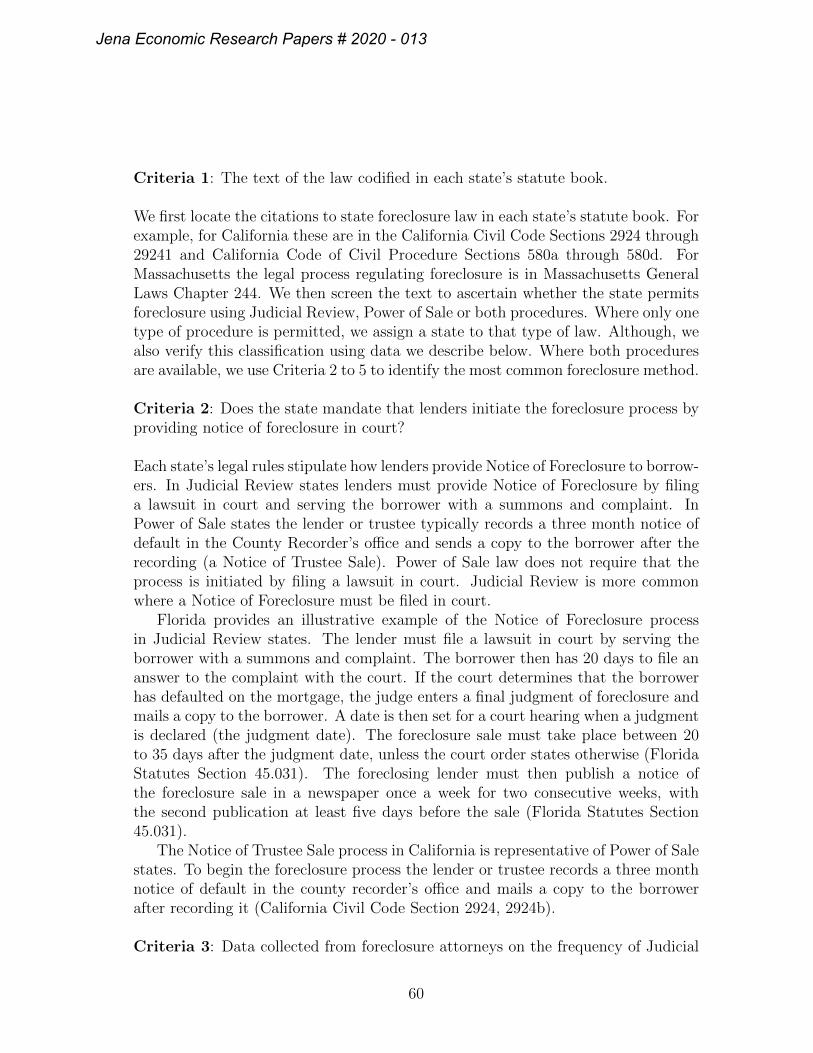
Criteria 1: The text of the law codified in each state’s statute book.
We first locate the citations to state foreclosure law in each state’s statute book. Forexample, for California these are in the California Civil Code Sections 2924 through29241 and California Code of Civil Procedure Sections 580a through 580d. ForMassachusetts the legal process regulating foreclosure is in Massachusetts GeneralLaws Chapter 244. We then screen the text to ascertain whether the state permitsforeclosure using Judicial Review, Power of Sale or both procedures. Where only onetype of procedure is permitted, we assign a state to that type of law. Although, wealso verify this classification using data we describe below. Where both proceduresare available, we use Criteria 2 to 5 to identify the most common foreclosure method.
Criteria 2: Does the state mandate that lenders initiate the foreclosure process byproviding notice of foreclosure in court?
Each state’s legal rules stipulate how lenders provide Notice of Foreclosure to borrow-ers. In Judicial Review states lenders must provide Notice of Foreclosure by filinga lawsuit in court and serving the borrower with a summons and complaint. InPower of Sale states the lender or trustee typically records a three month notice ofdefault in the County Recorder’s office and sends a copy to the borrower after therecording (a Notice of Trustee Sale). Power of Sale law does not require that theprocess is initiated by filing a lawsuit in court. Judicial Review is more commonwhere a Notice of Foreclosure must be filed in court.
Florida provides an illustrative example of the Notice of Foreclosure processin Judicial Review states. The lender must file a lawsuit in court by serving theborrower with a summons and complaint. The borrower then has 20 days to file ananswer to the complaint with the court. If the court determines that the borrowerhas defaulted on the mortgage, the judge enters a final judgment of foreclosure andmails a copy to the borrower. A date is then set for a court hearing when a judgmentis declared (the judgment date). The foreclosure sale must take place between 20to 35 days after the judgment date, unless the court order states otherwise (FloridaStatutes Section 45.031). The foreclosing lender must then publish a notice ofthe foreclosure sale in a newspaper once a week for two consecutive weeks, withthe second publication at least five days before the sale (Florida Statutes Section45.031).
The Notice of Trustee Sale process in California is representative of Power of Salestates. To begin the foreclosure process the lender or trustee records a three monthnotice of default in the county recorder’s office and mails a copy to the borrowerafter recording it (California Civil Code Section 2924, 2924b).
Criteria 3: Data collected from foreclosure attorneys on the frequency of Judicial
60
Jena Economic Research Papers # 2020 - 013
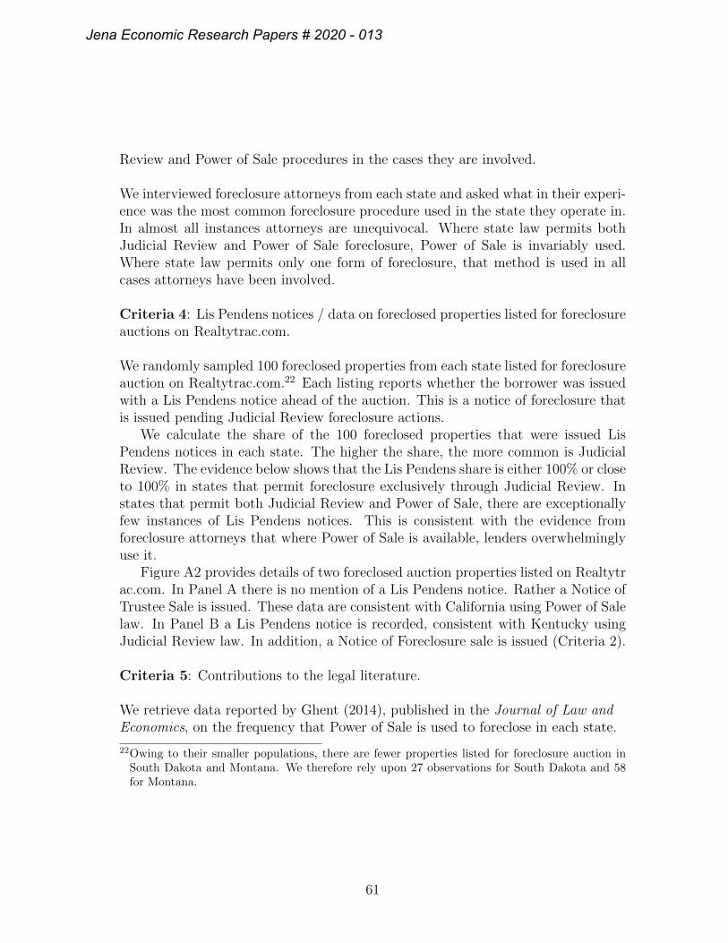
Review and Power of Sale procedures in the cases they are involved.
We interviewed foreclosure attorneys from each state and asked what in their experi-ence was the most common foreclosure procedure used in the state they operate in.In almost all instances attorneys are unequivocal. Where state law permits bothJudicial Review and Power of Sale foreclosure, Power of Sale is invariably used.Where state law permits only one form of foreclosure, that method is used in allcases attorneys have been involved.
Criteria 4: Lis Pendens notices / data on foreclosed properties listed for foreclosureauctions on Realtytrac.com.
We randomly sampled 100 foreclosed properties from each state listed for foreclosureauction on Realtytrac.com.22 Each listing reports whether the borrower was issuedwith a Lis Pendens notice ahead of the auction. This is a notice of foreclosure thatis issued pending Judicial Review foreclosure actions.
We calculate the share of the 100 foreclosed properties that were issued LisPendens notices in each state. The higher the share, the more common is JudicialReview. The evidence below shows that the Lis Pendens share is either 100% or closeto 100% in states that permit foreclosure exclusively through Judicial Review. Instates that permit both Judicial Review and Power of Sale, there are exceptionallyfew instances of Lis Pendens notices. This is consistent with the evidence fromforeclosure attorneys that where Power of Sale is available, lenders overwhelminglyuse it.
Figure A2 provides details of two foreclosed auction properties listed on Realtytrac.com. In Panel A there is no mention of a Lis Pendens notice. Rather a Notice ofTrustee Sale is issued. These data are consistent with California using Power of Salelaw. In Panel B a Lis Pendens notice is recorded, consistent with Kentucky usingJudicial Review law. In addition, a Notice of Foreclosure sale is issued (Criteria 2).
Criteria 5: Contributions to the legal literature.
We retrieve data reported by Ghent (2014), published in the Journal of Law andEconomics, on the frequency that Power of Sale is used to foreclose in each state.
22Owing to their smaller populations, there are fewer properties listed for foreclosure auction inSouth Dakota and Montana. We therefore rely upon 27 observations for South Dakota and 58for Montana.
61
Jena Economic Research Papers # 2020 - 013
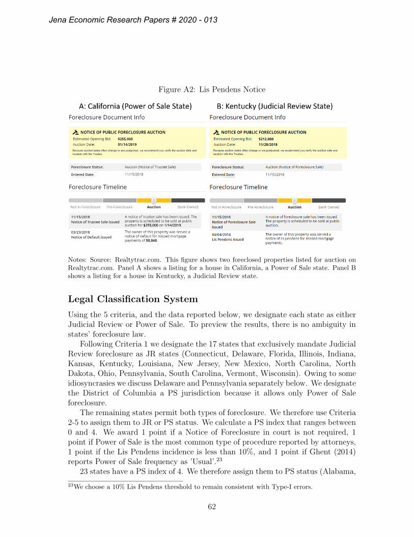
Figure A2: Lis Pendens Notice
Notes: Source: Realtytrac.com. This figure shows two foreclosed properties listed for auction onRealtytrac.com. Panel A shows a listing for a house in California, a Power of Sale state. Panel Bshows a listing for a house in Kentucky, a Judicial Review state.
Legal Classification System
Using the 5 criteria, and the data reported below, we designate each state as eitherJudicial Review or Power of Sale. To preview the results, there is no ambiguity instates’ foreclosure law.
Following Criteria 1 we designate the 17 states that exclusively mandate JudicialReview foreclosure as JR states (Connecticut, Delaware, Florida, Illinois, Indiana,Kansas, Kentucky, Louisiana, New Jersey, New Mexico, North Carolina, NorthDakota, Ohio, Pennsylvania, South Carolina, Vermont, Wisconsin). Owing to someidiosyncrasies we discuss Delaware and Pennsylvania separately below. We designatethe District of Columbia a PS jurisdiction because it allows only Power of Saleforeclosure.
The remaining states permit both types of foreclosure. We therefore use Criteria2-5 to assign them to JR or PS status. We calculate a PS index that ranges between0 and 4. We award 1 point if a Notice of Foreclosure in court is not required, 1point if Power of Sale is the most common type of procedure reported by attorneys,1 point if the Lis Pendens incidence is less than 10%, and 1 point if Ghent (2014)reports Power of Sale frequency as ’Usual’.23
23 states have a PS index of 4. We therefore assign them to PS status (Alabama,
23We choose a 10% Lis Pendens threshold to remain consistent with Type-I errors.
62
Jena Economic Research Papers # 2020 - 013

Alaska, Arizona, Arkansas, California, Georgia, Idaho, Michigan, Minnesota, Missis-sippi, Missouri, Montana, Nevada, New Hampshire, Oregon, Rhode Island, Tennessee,Texas, Utah, Virginia, Washington, West Virginia, and Wyoming).
3 states have a PS index of 3 (Colorado, Maryland, Massachusetts, and Nebraska).We assign them to PS status on the grounds that they meet the majority of our PScriteria. The reasons for these designations are:
Colorado only uses a Judicial Review process when the borrower is protectedunder the Service Members Civil Relief Act (known as a “Rule 120 hearing”).This applies exclusively to veterans and is seldom used. Power of Sale is thusthe default option. All other indicators are consistent with PS law.
Massachusetts state law mandates Lis Pendens notices are filed before a foreclos-ure auction, despite Power of Sale being the default method of foreclosure. SeeMassachusetts General Laws Chapter 184 Section 15(a)-(b). All other indicatorsare consistent with PS law.
Nebraska: Ghent (2014) reports Power of Sale as being ’Available’ rather than’Usual’. All other indicators are consistent with PS law.
6 states permit foreclosure using Judicial Review or Power of Sale and have PSindex values between 0 and 2. Iowa, Maine, and New York have a PS index of 0.Oklahoma has a PS index of 1. South Dakota has a PS index of 2. We assign allfive states to JR status because while Power of Sale is available, idiosyncrasies ofstate law effectively rule out Power of Sale.
Iowa (PS index = 0): we classify Iowa as a JR state. Although Iowa permitsPower of Sale, this procedure can only be used where borrowers voluntarilygive up possession of their home and the lender agrees to waive any deficiency.This type of procedure is rarely used. All other criteria are consistent withJudicial Review. For example, lenders file a Notice of Foreclosure in court, theLis Pendens incidence is 100%, attorneys report Judicial Review as the defaultoption, and Ghent (2014) reports Power of Sale as being ’Unavailable’.
Maine (PS index = 0): lenders must initiate a foreclosure by providing a Noticeof Foreclosure in court, attorneys report JR as the most common procedure,the Lis Pendens incidence is 100%, and Ghent (2014) reports Power of Sale as’Rare’. Maine has used Judicial Review historically such that it is the defaultoption.
New York (PS index = 0) has used Judicial Review law since at least the
63
Jena Economic Research Papers # 2020 - 013
1800s (Fox, 2015). Lenders must initiate a foreclosure by providing a Noticeof Foreclosure in court, attorneys report Judicial Review as the most commonprocedure, the Lis Pendens incidence is 100%, and Ghent (2014) reports Powerof Sale as ’Rare’. In essence, despite both foreclosure procedures being availablein New York, historical precedent means that only Judicial Review is used. Theclassification is consistent with the huge number of foreclosure cases and courtbacklogs in New York.
Maryland (PS index = 1): from criteria 2-5 all indicators are consistent withJudicial Review, except that Ghent (2014) reports the Power of Sale frequencyas usual. However, lenders must start the foreclosure process by filing a Notice ofForeclosure in the County Circuit court where the property is located, attorneysreport Judicial Review as the default procedure and a court must ratify theforeclosure sale, and the Lis Pendens incidence is 100%. Furthermore, Pence(2006), Demiroglu et al. (2014) and Ghent and Kudlyak (2011) classify Marylandas a Judicial Review state.
Oklahoma (PS index = 1): lenders do not have to file a Notice of Foreclosurein court. However, while Power of Sale is permitted, borrowers can force alender to use Judicial Review by sending a certified letter electing for judicialforeclosure to the lender and the county clerk’s office (Oklahoma Statute title46, Section 43). Delinquent borrowers have often chosen this route such thatlenders invariably use Judicial Review. All other criteria are consistent withJudicial Review law.
South Dakota (PS index = 2): we classify South Dakota as a Judicial Reviewstate because borrowers can easily challenge Power of Sale foreclosure and dema-nd the process is overseen by a judge (South Dakota Codified Laws Section21-48-9). Hence, while only 4% of foreclosed borrowers are issued with LisPendens notices, Power of Sale is rarely used. Ghent (2014) also reports Powerof Sale to be ’Rare’. Conversations with foreclosure attorneys confirm this.
Hawaii is the only state that effectively changes the type of foreclosure law it usesduring recent years. Hawaii permits foreclosure using both Judicial Review andPower of Sale. Before 2011 Power of Sale was the default option. However, Hawaiieffectively became a Judicial Review state in 2011 following the introduction of aMortgage Foreclosure Dispute Resolution program that applies exclusively to Powerof Sale foreclosures. This program brings borrowers and lenders together with thegoal of resolving mortgage default. This can result in a longer foreclosure timeline asthe borrower is granted time to find ways to avoid foreclosure. To avoid the burdensthis imposes, lenders now mainly foreclose using Judicial Review. This classification
64
Jena Economic Research Papers # 2020 - 013
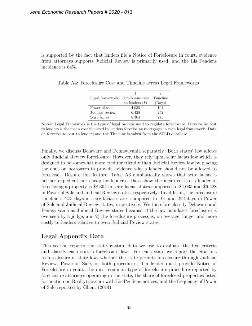
is supported by the fact that lenders file a Notice of Foreclosure in court, evidencefrom attorneys supports Judicial Review is primarily used, and the Lis Pendensincidence is 64%.
Table A4: Foreclosure Cost and Timeline across Legal Frameworks
1 2Legal framework Foreclosure cost Timeline
to lenders ($) (Days)Power of sale 4,035 101Judicial review 6,428 252Scire facias 8,304 275
Notes: Legal Framework is the type of legal process used to regulate foreclosure. Foreclosure costto lenders is the mean cost incurred by lenders foreclosing mortgages in each legal framework. Dataon foreclosure cost to lenders and the Timeline is taken from the SFLD database.
Finally, we discuss Delaware and Pennsylvania separately. Both states’ law allowsonly Judicial Review foreclosure. However, they rely upon scire facias law which isdesigned to be somewhat more creditor friendly than Judicial Review law by placingthe onus on borrowers to provide evidence why a lender should not be allowed toforeclose. Despite this feature, Table A3 emphatically shows that scire facias isneither expedient nor cheap for lenders. Data show the mean cost to a lender offoreclosing a property is $8,304 in scire facias states compared to $4,035 and $6,428in Power of Sale and Judicial Review states, respectively. In addition, the foreclosuretimeline is 275 days in scire facias states compared to 101 and 252 days in Powerof Sale and Judicial Review states, respectively. We therefore classify Delaware andPennsylvania as Judicial Review states because 1) the law mandates foreclosure isoverseen by a judge, and 2) the foreclosure process is, on average, longer and morecostly to lenders relative to even Judicial Review states.
Legal Appendix Data
This section reports the state-by-state data we use to evaluate the five criteriaand classify each state’s foreclosure law. For each state we report the citationsto foreclosure in state law, whether the state permits foreclosure through JudicialReview, Power of Sale, or both procedures, if a lender must provide Notice ofForeclosure in court, the most common type of foreclosure procedure reported byforeclosure attorneys operating in the state, the share of foreclosed properties listedfor auction on Realtytrac.com with Lis Pendens notices, and the frequency of Powerof Sale reported by Ghent (2014).
65
Jena Economic Research Papers # 2020 - 013
AlabamaCitations to state foreclosure law : Alabama Code Sections 35-10-1 to 35-10-30, andSections 6-5-247 to 6-5-257.Law available: Judicial Review & Power of Sale.Notice of Foreclosure in court : No.Most common type of procedure (attorneys): Power of Sale.Lis Pendens incidence: 0%.PS frequency (Ghent, 2014): Usual.
AlaskaCitations to state foreclosure law : Alaska Statutes Sections 34.20.070 to 34.20.100.Law available: Judicial Review & Power of Sale.Notice of Foreclosure in court : No.Most common type of procedure (attorneys): Power of Sale.Lis Pendens incidence: 0%.PS frequency (Ghent, 2014): Usual.
ArizonaCitations to state foreclosure law : Arizona Revised Statutes Sections 33-721 to33-730 (judicial), and Sections 33-801 to 33-821 (nonjudicial).Law available: Judicial Review & Power of Sale.Notice of Foreclosure in court : No.Most common type of procedure (attorneys): Power of Sale.Lis Pendens incidence: 0%.PS frequency (Ghent, 2014): Usual.
ArkansasCitations to state foreclosure law : Arkansas Code Annotated Sections 18-49-101through 18-49-106, and Sections 18-50-101 through 18-50-116.Law available: Judicial Review & Power of Sale.Notice of Foreclosure in court : No.Most common type of procedure (attorneys): Power of Sale.Lis Pendens incidence: 0%.PS frequency (Ghent, 2014): Usual.
CaliforniaCitations to state foreclosure law : California Civil Code Sections 2924 through 2924l,and California Code of Civil Procedure Sections 580a through 580d.Law available: Judicial Review & Power of Sale.Notice of Foreclosure in court : No.Most common type of procedure (attorneys): Power of Sale.
66
Jena Economic Research Papers # 2020 - 013
Lis Pendens incidence: 0%.PS frequency (Ghent, 2014): Usual.
ColoradoCitations to state foreclosure law : Colorado Revised Statutes Sections 38-38-100.3through 38-38-114.Law available: Judicial Review & Power of Sale.Notice of Foreclosure in court : No.Most common type of procedure (attorneys): Power of Sale. There is some minimalcourt involvement when the attorney representing the foreclosing party files a motionunder Rule 120 of the Colorado Rules of Civil Procedure asking a court for an orderauthorizing the foreclosure sale by the public trustee. The court sets a hearing (calleda “Rule 120 hearing”), which is limited to an inquiry of whether the borrower is indefault and in the military and subject to protections under the Service MembersCivil Relief Act. Neither of these issues is typically in dispute, such that Rule 120hearings do not need to take place and the court enters the requested order.Lis Pendens incidence: 0%.PS frequency (Ghent, 2014): Usual.
ConnecticutCitations to state foreclosure law : Connecticut General Statutes Title 49, Sections49-1 through 49-31v, and Connecticut Superior Court Rules 23-16 through 23-19.Law available: Judicial Review.Notice of Foreclosure in court : Yes. The foreclosing party starts the foreclosureby filing a complaint with the court and serving it to the borrower along with asummons.Most common type of procedure (attorneys): Judicial Review. Foreclosures areeither by sale (where the court orders the home sold and the proceeds paid tothe foreclosing party to satisfy the outstanding debt) or strict foreclosure (wherethe court transfers title to the home directly to the foreclosing party without aforeclosure sale). Connecticut Geneneral Statutes Section 49-24.Lis Pendens incidence: 100%.PS frequency (Ghent, 2014): Unavailable.
DelawareCitations to state foreclosure law : Delaware Code Annotated Title 10, Chapter 49,Sections 5061 through 5067.Law available: Judicial Review.Notice of Foreclosure in court : Yes. To officially start the foreclosure, the foreclosingparty files a lawsuit in court and provides notice of the suit to the borrower by servinghim or her with a summons and complaint.
67
Jena Economic Research Papers # 2020 - 013

Most common type of procedure (attorneys): Judicial Review. The lender must suethe borrower in court in order to foreclose.Lis Pendens incidence: 100%.PS frequency (Ghent, 2014): Unavailable.
District of ColumbiaCitations to state foreclosure law : District of Columbia Code Sections 42-815 through42-816.Law available: Power of Sale.Notice of Foreclosure in court : No.Most common type of procedure (attorneys): Power of Sale.Lis Pendens incidence: 0%.PS frequency (Ghent, 2014): Usual.
FloridaCitations to state foreclosure law : Florida Statutes Sections 702.01 through 702.11,and Sections 45.031 through 45.0315.Law available: Judicial Review.Notice of Foreclosure in court : Yes. The foreclosing party files a lawsuit in court tostart the foreclosure and gives notice of the lawsuit by serving the borrower with asummons and complaint.Most common type of procedure (attorneys): Judicial Review.Lis Pendens incidence: 100%.PS frequency (Ghent, 2014): Unavailable.
GeorgiaCitations to state foreclosure law : Georgia Code Annotated Sections 44-14-160through 44-14-191.Law available: Judicial Review & Power of Sale.Notice of Foreclosure in court : No.Most common type of procedure (attorneys): Power of Sale.Lis Pendens incidence: 0%.PS frequency (Ghent, 2014): Usual.
HawaiiCitations to state foreclosure law : Hawaii Revised Statutes Sections 667-1.5 through667-20.1 (judicial), and Sections 667-21 through 667-41 (nonjudicial).Law available: Judicial Review & Power of Sale.Notice of Foreclosure in court : Required if a lender opts for foreclosure using JudicialReview.Most common type of procedure (attorneys): Power of Sale (until 2011), Judicial
68
Jena Economic Research Papers # 2020 - 013
Review (post 2011). The state implemented a Mortgage Foreclosure Dispute Resolu-tion Program in 2011 which applies to Power of Sale foreclosures. To bypass themediation program, most lenders now use Judicial Review.Lis Pendens incidence: 64%.PS frequency (Ghent, 2014): Available.
IdahoCitations to state foreclosure law : Idaho Code Sections 45-1505 through 45-1515.Law available: Judicial Review & Power of Sale.Notice of Foreclosure in court : No.Most common type of procedure (attorneys): Power of Sale.Lis Pendens incidence: 0%.PS frequency (Ghent, 2014): Usual.
IllinoisCitations to state foreclosure law : Illinois Compiled Statutes Chapter 735, Sections5/15-1501 through 5/15-1605.Law available: Judicial Review.Notice of Foreclosure in court : Yes. To begin the foreclosure, the foreclosing partyfiles a lawsuit and gives notice of the suit by serving the borrower with a complaintand summons, along with a notice that advises the homeowner of his or her rightsduring the foreclosure process.Most common type of procedure (attorneys): Judicial Review.Lis Pendens incidence: 100%.PS frequency (Ghent, 2014): Unavailable.
IndianaCitations to state foreclosure law : Indiana Code Sections 32-30-10-1 through 32-30-10-14, Sections 32-29-1-1 through 32-29-1-11, and Sections 32-29-7-1 through 32-29-7-14.Law available: Judicial Review.Notice of Foreclosure in court : Yes. The foreclosing party gives the lender notice ofthe lawsuit by serving a court summons and complaint.Most common type of procedure (attorneys): Judicial Review.Lis Pendens incidence: 100%.PS frequency (Ghent, 2014): Unavailable.
IowaCitations to state foreclosure law : Iowa Code Sections 654.1 through 654.26, andSections 655A.1 through 655A.9.Law available: Judicial Review & Power of Sale.Notice of Foreclosure in court : To officially start the foreclosure, the lender files a
69
Jena Economic Research Papers # 2020 - 013
lawsuit in court.Most common type of procedure (attorneys): Judicial Review. Iowa law also allowsan alternative non-judicial voluntary foreclosures (where the borrower voluntarilygives up possession of the home and the lender agrees to waive any deficiency).However, these non-judicial procedures rarely occur.Lis Pendens incidence: 100%.PS frequency (Ghent, 2014): Unavailable.
KansasCitations to state foreclosure law : Kansas Statutes Annotated Sections 60-2410,60-2414, and 60-2415.Law available: Judicial Review.Notice of Foreclosure in court : The lender starts the foreclosure process by filing alawsuit in court.Most common type of procedure (attorneys): Judicial Review.Lis Pendens incidence: 100%.PS frequency (Ghent, 2014): Unavailable.
KentuckyCitations to state foreclosure law : Chapter 426 of the Kentucky Revised Statutes.Law available: Judicial Review.Notice of Foreclosure in court : Yes. The foreclosing party gives the borrower noticeof the lawsuit by serving him or her with a summons and complaint.Most common type of procedure (attorneys): Judicial Review.Lis Pendens incidence: 100%.PS frequency (Ghent, 2014): Unavailable.
LouisianaCitations to state foreclosure law : Louisiana Code of Civil Procedure Articles 3721through 3753, Articles 2631 through 2772, and Louisiana Revised Statutes Section13:3852.Law available: Judicial Review.Notice of Foreclosure in court : Upon a default, the foreclosing party files a foreclosurepetition in court with the mortgage attached and the court orders the property seizedand sold. The homeowner can fight the foreclosure only by appealing or bringing alawsuit.Most common type of procedure (attorneys): Judicial Review.Lis Pendens incidence: 100%.PS frequency (Ghent, 2014): Unavailable.
Maine
70
Jena Economic Research Papers # 2020 - 013
Citations to state foreclosure law : Maine Revised Statutes Title 14 Sections 6101through 6325.Law available: Judicial Review & Power of Sale.Notice of Foreclosure in court : Yes. To officially start the foreclosure, the foreclosingparty files a lawsuit in court and gives notice of the suit by serving the borrower asummons and complaint.Most common type of procedure (attorneys): Judicial Review.Lis Pendens incidence: 100%.PS frequency (Ghent, 2014): Rare.
MarylandCitations to state foreclosure law : Code of Maryland (Real Property) Sections 7-105through 7-105.8, Maryland Rules 14-201 through 14-209, and Rules 14-305 through14-306.Law available: Judicial Review & Power of Sale.Notice of Foreclosure in court : Yes. The lender initiates a foreclosure case with theCircuit Court in the county in which the property is located.Most common type of procedure (attorneys): Judicial Review.Lis Pendens incidence: 100%.PS frequency (Ghent, 2014): Usual.
MassachusettsCitations to state foreclosure law : Massachusetts General Laws Chapter 244.Law available: Judicial Review & Power of Sale.Notice of Foreclosure in court : No.Most common type of procedure (attorneys): Power of Sale.Lis Pendens incidence: 99%.PS frequency (Ghent, 2014): Usual.
MichiganCitations to state foreclosure law : Michigan Compiled Laws Sections 600.3101 through600.3185, and Sections 600.3201 through 600.3285.Law available: Judicial Review & Power of Sale.Notice of Foreclosure in court : No.Most common type of procedure (attorneys): Power of Sale.Lis Pendens incidence: 0%.PS frequency (Ghent, 2014): Usual.
MinnesotaCitations to state foreclosure law : Minnesota Statutes Sections 580.01 through580.30 (foreclosure by advertisement), Sections 581.01 through 581.12 (foreclosure
71
Jena Economic Research Papers # 2020 - 013
by action), and Sections 582.01 through 582.32 (general foreclosure provisions).Law available: Judicial Review & Power of Sale.Notice of Foreclosure in court : No.Most common type of procedure (attorneys): Power of Sale.Lis Pendens incidence: 0%PS frequency (Ghent, 2014): Usual
MississippiCitations to state foreclosure law : Mississippi Code Annotated Sections 89-1-55through 89-1-59.Law available: Judicial Review & Power of Sale.Notice of Foreclosure in court : No.Most common type of procedure (attorneys): Power of Sale.Lis Pendens incidence: 0%.PS frequency (Ghent, 2014): Usual.
MissouriCitations to state foreclosure law : Missouri Revised Statutes Sections 443.290 through443.440 (nonjudicial foreclosures), and Missouri Revised Statutes Section 443.190and 443.280 (judicial foreclosures).Law available: Judicial Review & Power of Sale.Notice of Foreclosure in court : No.Most common type of procedure (attorneys): Power of Sale.Lis Pendens incidence: 0%.PS frequency (Ghent, 2014): Usual.
MontanaCitations to state foreclosure law : Montana Code Annotated Sections 71-1-221through 71-1-235, and Sections 71-1-301 through 71-1-321.Law available: Judicial Review & Power of Sale.Notice of Foreclosure in court : No.Most common type of procedure (attorneys): Power of sale. Home mortgages inMontana are trust indentures (also known as deeds of trust) under the state’s SmallTract Financing Act, which is for properties that do not exceed 40 acres. This typeof mortgage can be foreclosed nonjudicially (without a lawsuit) or judicially (witha lawsuit). However, non-judicial foreclosure is the default option.Lis Pendens incidence: 0%.PS frequency (Ghent, 2014): Usual.
NebraskaCitations to state foreclosure law : Nebraska Revised Statutes Sections 76-1005
72
Jena Economic Research Papers # 2020 - 013
through 76-1018 (nonjudicial), and Sections 25-2137 through 25-2155 (judicial).Law available: Judicial Review & Power of Sale.Notice of Foreclosure in court : No.Most common type of procedure (attorneys): Power of Sale.Lis Pendens incidence: 0%.PS frequency (Ghent, 2014): Available.
NevadaCitations to state foreclosure law : Nevada Revised Statutes Sections 107.0795 through107.130, Sections 40.430 through 40.450, and Sections 40.451 through 40.463.Law available: Judicial Review & Power of Sale.Notice of Foreclosure in court : No.Most common type of procedure (attorneys): Power of Sale.Lis Pendens incidence: 0%.PS frequency (Ghent, 2014): Usual.
New HampshireCitations to state foreclosure law : Title XLVIII, Chapter 479 of the New HampshireRevised Statutes.Law available: Judicial Review & Power of Sale.Notice of Foreclosure in court : No.Most common type of procedure (attorneys): Power of Sale.Lis Pendens incidence: 0%.PS frequency (Ghent, 2014): Usual.
New JerseyCitations to state foreclosure law : New Jersey Statutes Annotated Sections 2A:50-1through 2A:50-21 and Sections 2A:50-53 through 2A:50-63.Law available: Judicial Review.Notice of Foreclosure in court : Yes. The foreclosing party starts the foreclosureprocess by filing a lawsuit in court and giving notice of the suit by serving theborrower with a summons and complaint.Most common type of procedure (attorneys): Judicial Review.Lis Pendens incidence: 100%.PS frequency (Ghent, 2014): Unavailable.
New MexicoCitations to state foreclosure law : New Mexico Statutes Sections 48-7-1 through48-7-24, Sections 39-5-1 through 39-5-23, and Sections 48-10-1 through 48-10-21.Law available: Judicial ReviewNotice of Foreclosure in court : Yes. The foreclosing party officially starts a judicial
73
Jena Economic Research Papers # 2020 - 013
foreclosure by filing a lawsuit (a complaint) in court.Most common type of procedure (attorneys): Judicial review. Nonjudicial foreclosuresare also possible, but uncommon.Lis Pendens incidence: 100%.PS frequency (Ghent, 2014): Available only for deeds of trust.
New YorkCitations to state foreclosure law : New York Real Property Actions & ProceedingsSections 1301 through 1391.Law available: Judicial Review & Power of Sale.Notice of Foreclosure in court : Yes. The foreclosing party officially starts theforeclosure process by filing a lawsuit (a complaint) in court. It gives notice ofthe lawsuit to the borrower by serving him or her with a summons and complaint,along with notices advising the borrower about the foreclosure process.Most common type of procedure (attorneys): Judicial Review.Lis Pendens incidence: 100%.PS frequency (Ghent, 2014): Rare.
North CarolinaCitations to state foreclosure law : North Carolina General Statutes Sections 45-21.1through 45-21.38C, and Sections 45-100 through 107.Law available: Judicial Review & Power of Sale.Notice of Foreclosure in court : No. However, to officially start the foreclosure, theforeclosing party files a notice of hearing with the court clerk.Most common type of procedure (attorneys): Power of Sale.Lis Pendens incidence: 0%.PS frequency (Ghent, 2014): Usual.
North DakotaCitations to state foreclosure law : North Dakota Century Code Sections 32-19-01through 32-19-41, and Sections 28-23-04 to 28-23-14.Law available: Judicial ReviewNotice of Foreclosure in court : Yes. The foreclosing party officially starts theforeclosure by filing a lawsuit (a complaint) in court. It gives notice of the lawsuitto the borrower by serving him or her with a summons and complaint.Most common type of procedure (attorneys): Judicial Review.Lis Pendens incidence: 100%.PS frequency (Ghent, 2014): Unavailable.
OhioCitations to state foreclosure law : Title 23, Chapter 2323 (Section 2323.07) and
74
Jena Economic Research Papers # 2020 - 013
Chapter 2329 of the Ohio Revised Code.Law available: Judicial Review.Notice of Foreclosure in court : Yes. The foreclosing party files a lawsuit to beginthe process and gives the borrower notice of the suit by serving him or her with asummons and complaint.Most common type of procedure (attorneys): Judicial Review.Lis Pendens incidence: 100%.PS frequency (Ghent, 2014): Unavailable.
OklahomaCitations to state foreclosure law : Oklahoma Statutes Title 12 Sections 686, 764through 765, 773, and Sections 41 through 49.Law available: Judicial Review & Power of Sale.Notice of Foreclosure in court : No.Most common type of procedure (attorneys): Judicial Review. Foreclosure cantake place using Power of Sale if the mortgage contract includes a power of saleclause. However, borrowers can force the lender to foreclose using Judicial Reviewby taking the following steps at least ten days before the date of the foreclosuresale: 1) notify the foreclosing party (the lender or servicer) by certified mail thatthe property to be sold is their homestead (primary residence) and that they electfor judicial foreclosure, and 2) record a copy of the notice in the county clerk’soffice (Oklahoma Statute title 46, Section 43). Judicial review is the most commonforeclosure procedure.Lis Pendens incidence: 100%.PS frequency (Ghent, 2014): Rare.
OregonCitations to state foreclosure law : Oregon Revised Statutes Sections 86.726 through86.815 (nonjudicial foreclosures), and Sections 88.010 through 88.106 (judicial forecl-osures).Law available: Judicial Review & Power of Sale.Notice of Foreclosure in court : No.Most common type of procedure (attorneys): Power of Sale.Lis Pendens incidence: 0%.PS frequency (Ghent, 2014): Usual.
PennsylvaniaCitations to state foreclosure law : Pennsylvania Statutes Annotated Title 35, Sections1680.402c to 1680.409c, Section 41, Sections 403 to 404, and Pennsylvania Rules ofCivil Procedure, Rules 1141-1150.Law available: Judicial Review.
75
Jena Economic Research Papers # 2020 - 013
Notice of Foreclosure in court : Yes. The foreclosing party officially starts theforeclosure process by filing a lawsuit (a complaint) in court. It gives notice ofthe lawsuit to the borrower by serving him or her with a summons and complaint.Most common type of procedure (attorneys): Judicial Review (scire facias).Lis Pendens incidence: 100%,PS frequency (Ghent, 2014): Unavailable.
Rhode IslandCitations to state foreclosure law : Rhode Island General Laws Sections 34-27-1through 34-27-5, and Sections 34-25.2-1 through 34-25.2-15.Law available: Judicial Review & Power of Sale.Notice of Foreclosure in court : No.Most common type of procedure (attorneys): Power of Sale.Lis Pendens incidence: 0%.PS frequency (Ghent, 2014): Usual.
South CarolinaCitations to state foreclosure law : South Carolina Code Sections 15-39-650 through15-39-660, and Sections 29-3-630 through 29-3-790.Law available: Judicial Review.Notice of Foreclosure in court : Yes. The lender must give the borrower notice ofthe lawsuit by serving a summons and complaint.Most common type of procedure (attorneys): Judicial Review.Lis Pendens incidence: 100%.PS frequency (Ghent, 2014): Unavailable.
South DakotaCitations to state foreclosure law : South Dakota Codified Laws Sections 21-47-1through 21-47-25 (judicial foreclosures), and Sections 21-48-1 through 21-48-26 (nonj-udicial foreclosures).Law available: Judicial Review & Power of Sale.Notice of Foreclosure in court : No.Most common type of procedure (attorneys): Judicial Review. Foreclosures in SouthDakota can be through Power of Sale. However, even if the lender starts a Powerof Sale foreclosure, the borrower can require the lender to foreclose using JudicialReview by making an application in the appropriate court (South Dakota CodifiedLaws Section 21-48-9).Lis Pendens incidence: 4%.PS frequency (Ghent, 2014): Rare.
Tennessee
76
Jena Economic Research Papers # 2020 - 013
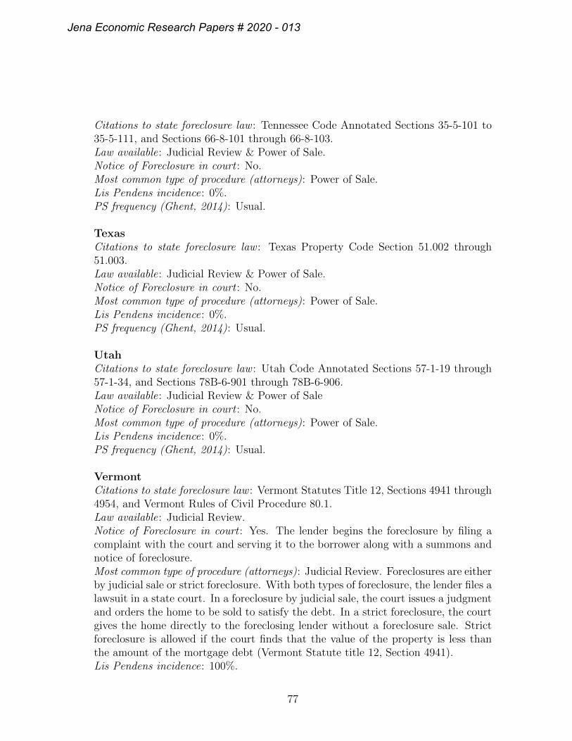
Citations to state foreclosure law : Tennessee Code Annotated Sections 35-5-101 to35-5-111, and Sections 66-8-101 through 66-8-103.Law available: Judicial Review & Power of Sale.Notice of Foreclosure in court : No.Most common type of procedure (attorneys): Power of Sale.Lis Pendens incidence: 0%.PS frequency (Ghent, 2014): Usual.
TexasCitations to state foreclosure law : Texas Property Code Section 51.002 through51.003.Law available: Judicial Review & Power of Sale.Notice of Foreclosure in court : No.Most common type of procedure (attorneys): Power of Sale.Lis Pendens incidence: 0%.PS frequency (Ghent, 2014): Usual.
UtahCitations to state foreclosure law : Utah Code Annotated Sections 57-1-19 through57-1-34, and Sections 78B-6-901 through 78B-6-906.Law available: Judicial Review & Power of SaleNotice of Foreclosure in court : No.Most common type of procedure (attorneys): Power of Sale.Lis Pendens incidence: 0%.PS frequency (Ghent, 2014): Usual.
VermontCitations to state foreclosure law : Vermont Statutes Title 12, Sections 4941 through4954, and Vermont Rules of Civil Procedure 80.1.Law available: Judicial Review.Notice of Foreclosure in court : Yes. The lender begins the foreclosure by filing acomplaint with the court and serving it to the borrower along with a summons andnotice of foreclosure.Most common type of procedure (attorneys): Judicial Review. Foreclosures are eitherby judicial sale or strict foreclosure. With both types of foreclosure, the lender files alawsuit in a state court. In a foreclosure by judicial sale, the court issues a judgmentand orders the home to be sold to satisfy the debt. In a strict foreclosure, the courtgives the home directly to the foreclosing lender without a foreclosure sale. Strictforeclosure is allowed if the court finds that the value of the property is less thanthe amount of the mortgage debt (Vermont Statute title 12, Section 4941).Lis Pendens incidence: 100%.
77
Jena Economic Research Papers # 2020 - 013
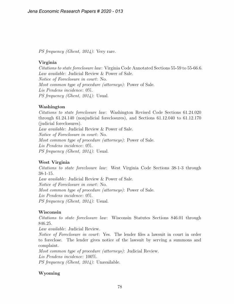
PS frequency (Ghent, 2014): Very rare.
VirginiaCitations to state foreclosure law : Virginia Code Annotated Sections 55-59 to 55-66.6.Law available: Judicial Review & Power of Sale.Notice of Foreclosure in court : No.Most common type of procedure (attorneys): Power of Sale.Lis Pendens incidence: 0%.PS frequency (Ghent, 2014): Usual.
WashingtonCitations to state foreclosure law : Washington Revised Code Sections 61.24.020through 61.24.140 (nonjudicial foreclosures), and Sections 61.12.040 to 61.12.170(judicial foreclosures).Law available: Judicial Review & Power of Sale.Notice of Foreclosure in court : No.Most common type of procedure (attorneys): Power of Sale.Lis Pendens incidence: 0%.PS frequency (Ghent, 2014): Usual.
West VirginiaCitations to state foreclosure law : West Virginia Code Sections 38-1-3 through38-1-15.Law available: Judicial Review & Power of Sale.Notice of Foreclosure in court : No.Most common type of procedure (attorneys): Power of Sale.Lis Pendens incidence: 0%.PS frequency (Ghent, 2014): Usual.
WisconsinCitations to state foreclosure law : Wisconsin Statutes Sections 846.01 through846.25.Law available: Judicial Review.Notice of Foreclosure in court : Yes. The lender files a lawsuit in court in orderto foreclose. The lender gives notice of the lawsuit by serving a summons andcomplaint.Most common type of procedure (attorneys): Judicial Review.Lis Pendens incidence: 100%.PS frequency (Ghent, 2014): Unavailable.
Wyoming
78
Jena Economic Research Papers # 2020 - 013
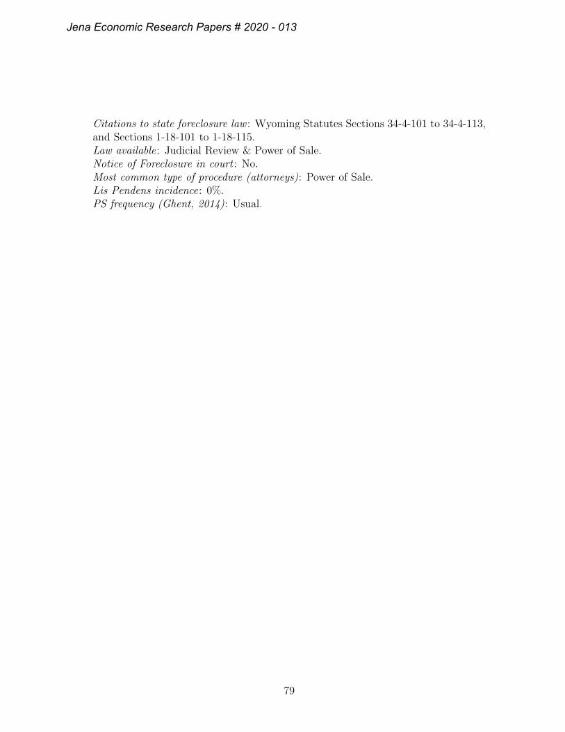
Citations to state foreclosure law : Wyoming Statutes Sections 34-4-101 to 34-4-113,and Sections 1-18-101 to 1-18-115.Law available: Judicial Review & Power of Sale.Notice of Foreclosure in court : No.Most common type of procedure (attorneys): Power of Sale.Lis Pendens incidence: 0%.PS frequency (Ghent, 2014): Usual.
79
Jena Economic Research Papers # 2020 - 013
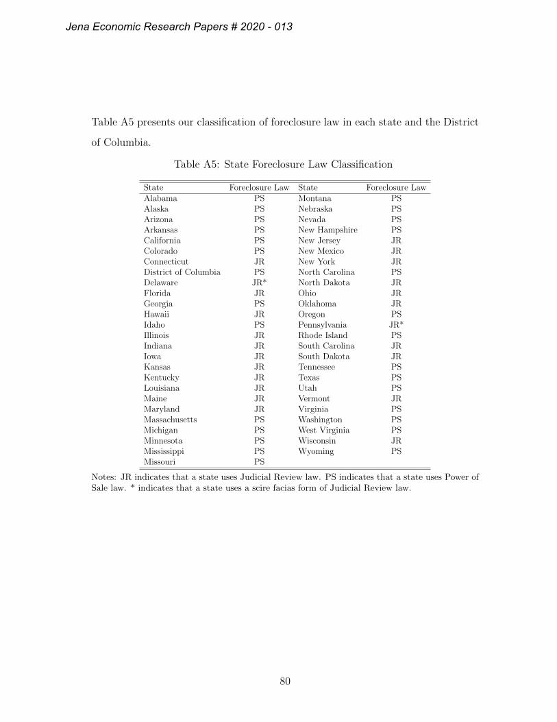
Table A5 presents our classification of foreclosure law in each state and the District
of Columbia.
Table A5: State Foreclosure Law Classification
State Foreclosure Law State Foreclosure LawAlabama PS Montana PSAlaska PS Nebraska PSArizona PS Nevada PSArkansas PS New Hampshire PSCalifornia PS New Jersey JRColorado PS New Mexico JRConnecticut JR New York JRDistrict of Columbia PS North Carolina PSDelaware JR* North Dakota JRFlorida JR Ohio JRGeorgia PS Oklahoma JRHawaii JR Oregon PSIdaho PS Pennsylvania JR*Illinois JR Rhode Island PSIndiana JR South Carolina JRIowa JR South Dakota JRKansas JR Tennessee PSKentucky JR Texas PSLouisiana JR Utah PSMaine JR Vermont JRMaryland JR Virginia PSMassachusetts PS Washington PSMichigan PS West Virginia PSMinnesota PS Wisconsin JRMississippi PS Wyoming PSMissouri PS
Notes: JR indicates that a state uses Judicial Review law. PS indicates that a state uses Power ofSale law. * indicates that a state uses a scire facias form of Judicial Review law.
80
Jena Economic Research Papers # 2020 - 013
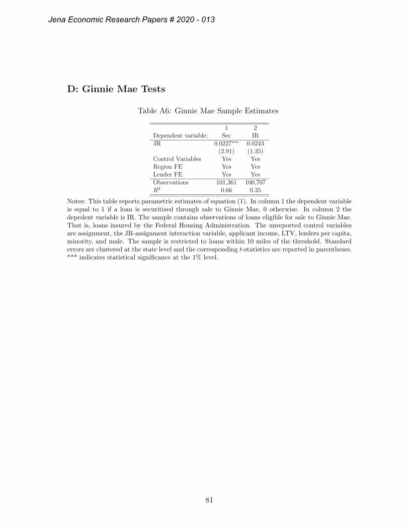
D: Ginnie Mae Tests
Table A6: Ginnie Mae Sample Estimates
1 2Dependent variable: Sec IRJR 0.0227∗∗∗ 0.0243
(2.91) (1.35)Control Variables Yes YesRegion FE Yes YesLender FE Yes YesObservations 101,361 100,707R2 0.66 0.35
Notes: This table reports parametric estimates of equation (1). In column 1 the dependent variableis equal to 1 if a loan is securitized through sale to Ginnie Mae, 0 otherwise. In column 2 thedepedent variable is IR. The sample contains observations of loans eligible for sale to Ginnie Mae.That is, loans insured by the Federal Housing Administration. The unreported control variablesare assignment, the JR-assignment interaction variable, applicant income, LTV, lenders per capita,minority, and male. The sample is restricted to loans within 10 miles of the threshold. Standarderrors are clustered at the state level and the corresponding t-statistics are reported in parentheses.*** indicates statistical significance at the 1% level.
81
Jena Economic Research Papers # 2020 - 013
E: Sensitivity Checks
E.1: Tests using 2000 to 2017 data
A natural question is whether our findings are specific to the year 2018. Our choice
to focus on this year is due to a lack of information on interest rates and other loan
characteristics in previous HMDA vintages. To examine the effects of JR law during
the years 2000 to 2017 we rely on HMDA for
1. Securitization of GSE-eligible loans
2. Securitization of non-GSE-eligible loans (subprime and jumbos)
3. Interest rates on non-GSE-eligible loans (subprime)
HMDA data limitations prevent observation of interest rates on GSE-eligible
loans and jumbo loans. We therefore rely exclusively on subprime loans (that
account for the majority of non-GSE-eligible loans) to inspect the pricing effects
of JR law in the non-GSE-eligible market. Interest rates are calculated using the
HMDA rate spread variable. The rate spread measures the difference between the
annual percentage rate (APR) on a loan and the average interest rate on prime
loans. We therefore calculate IR for non-GSE-eligible loans in year t as the sum
of the rate spread and average prime offer rate provided by the Federal Financial
Institutions Examination Council during year t. Information on the interest rate at
the point of origination on GSE-eligible loans is taken from the Fannie Mae Single
Family Loan database (SFLD).
Pooling annual HMDA and SFLD data results in a data set that is computationally
too large. In addition to the sample screens we apply to the 2018 data, we take a
10% random sample of the data sets. To mirror the previous econometric set-up,
we include region-year and lender-year fixed effects in equation (1). The LATEs
are therefore computed through cross-sectional comparisons of the treatment and
control groups at the same point in time within the same region.
82
Jena Economic Research Papers # 2020 - 013
The results in Table A7 are qualitatively and quantitatively similar to the estimat-
es from the 2018 data set. Consistent with the persistently higher credit risk of JR
law through time, the inferences also exist before and after the financial crisis.
83
Jena Economic Research Papers # 2020 - 013
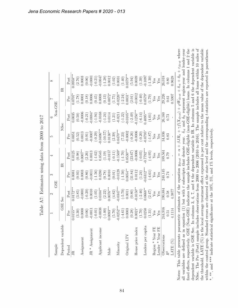
Tab
leA
7:E
stim
ates
usi
ng
dat
afr
om20
00to
2017
12
34
56
78
Sam
ple
GSE
Non
-GSE
Dep
enden
tva
riab
leG
SE
Sec
IRN
Sec
IR
Per
iod
Pre
Pos
tP
reP
ost
Pre
Pos
tP
reP
ost
JR
0.01
55∗∗
∗0.
0172
∗∗∗
0.00
810.
0125
0.00
510.
0035
0.07
07∗
0.09
58∗∗
∗
(3.3
0)(3
.85)
(0.9
3)(0
.98)
(0.5
2)(0
.50)
(1.7
8)(2
.76)
Ass
ignm
ent
0.00
00-0
.000
10.
0003
0.00
07∗∗
0.00
13-0
.000
60.
0001
0.00
03(0
.06)
(-0.
20)
(0.8
6)(2
.26)
(0.9
1)(-
0.21
)(0
.18)
(0.0
6)JR
*A
ssig
nm
ent
-0.0
011
0.00
10-0
.001
10.
0013
-0.0
007
-0.0
084∗
0.00
06-0
.000
1(-
0.01
)(1
.05)
(-1.
56)
(-1.
62)
(-0.
29)
(-1.
94)
(0.4
5)(-
0.21
)A
pplica
nt
inco
me
-0.0
038
0.01
04∗∗
0.02
800.
0545
-0.0
496∗
∗∗-0
.016
80.
0008
-0.0
047
(-1.
00)
(2.2
2)(0
.78)
(1.1
9)(-
10.5
7)(-
1.24
)(0
.13)
(-1.
28)
Mal
e0.
0093
∗∗∗
0.00
76∗∗
∗0.
0010
-0.0
157
0.01
30∗∗
0.01
140.
0072
∗0.
0012
(5.7
0)(4
.82)
(0.0
1)(-
0.11
)(2
.39)
(1.2
1)(1
.75)
(1.0
2)M
inor
ity
-0.0
252∗
∗∗-0
.034
7∗∗∗
-0.0
128
-0.1
569∗
0.04
70∗∗
∗-0
.021
1-0
.022
6∗∗
0.00
31(-
4.61
)(-
5.70
)(-
1.50
)(-
1.70
)(7
.23)
(-1.
22)
(-2.
24)
(1.4
0)O
rigi
nal
LT
V0.
0003
0.00
110.
0054
∗∗0.
0530
∗∗∗
-0.0
002
-0.0
105∗
∗0.
0031
∗0.
0379
∗∗∗
(0.2
8)(0
.80)
(31.
84)
(23.
67)
(-0.
26)
(-2.
49)
(2.0
1)(5
.94)
Hou
sepri
cein
dex
0.00
21∗
-0.0
150∗
∗0.
0112
-0.0
006
-0.0
006
-0.1
256∗
∗∗-0
.001
20.
0039
(1.7
0)(-
2.46
)(1
.24)
(-0.
05)
(-0.
20)
(-6.
14)
(-0.
40)
(1.3
9)L
ender
sp
erca
pit
a0.
0250
0.06
68∗∗
-0.6
312∗
∗∗-0
.779
2∗∗∗
-0.0
795∗
0.40
95∗∗
∗0.
0579
∗-0
.109
7(1
.31)
(2.4
7)(-
4.61
)(-
4.95
)(-
1.87
)(4
.01)
(1.7
9)(-
1.30
)R
egio
n*
Yea
rF
EY
esY
esY
esY
esY
esY
esY
esY
esL
ender
*Y
ear
FE
Yes
Yes
Yes
Yes
Yes
Yes
Yes
Yes
Obse
rvat
ions
244,
916
190,
884
240,
145
189,
561
34,0
3626
,160
29,2
2626
,018
R2
0.51
0.58
0.74
0.79
0.83
0.73
0.61
0.80
LA
TE
(%)
4.11
144.
3877
--
--
0.59
070.
9628
Not
es:
Th
ista
ble
pre
sents
par
am
etri
ces
tim
ates
ofth
eeq
uat
iony i
lrst
=α
+βJR
s+γf
(Xilrst)
+ϕW
ilrst
+δ r
t+δ l
t+ε i
lrst
wh
ere
all
vari
able
sar
ed
efined
asin
equ
atio
n(1
)b
ut
wit
ht
sub
scri
pts
that
den
ote
year
.δ r
tan
dδ l
tre
pre
sent
regi
on-y
ear
and
len
der
-yea
rfi
xed
effec
ts,
resp
ecti
vely
.G
SE
(Non
-GS
E)
ind
icat
esth
esa
mp
lein
clu
des
GS
E-e
ligi
ble
(non
-GS
E-e
ligi
ble
)lo
ans.
Inco
lum
ns
1an
d2
the
dep
end
ent
vari
able
isG
SE
Sec
.In
colu
mn
s3,
4,7,
and
8th
edep
end
ent
vari
able
isIR
.In
colu
mn
s5
and
6th
ed
epen
den
tva
riab
leis
NS
ec.
Th
eP
re(P
ost)
sam
ple
incl
ud
esob
serv
atio
ns
from
2000
to20
06(2
010
to20
16).
Th
esa
mp
lein
clu
des
all
loan
sw
ith
in10
mil
esof
the
thre
shol
d.
LA
TE
(%)
isth
elo
cal
aver
age
trea
tmen
teff
ect
exp
ress
edin
per
cent
rela
tive
toth
em
ean
valu
eof
the
dep
end
ent
vari
able
wit
hin
the
contr
olgr
oup
.S
tan
dar
der
rors
are
clu
ster
edat
the
stat
ele
vel
and
the
corr
esp
ond
ingt-
stat
isti
csar
ere
por
ted
inp
aren
thes
es.
*,**
,an
d**
*in
dic
ate
stat
isti
cal
sign
ifica
nce
atth
e10
%,
5%,
and
1%le
vel
s,re
spec
tive
ly.
84
Jena Economic Research Papers # 2020 - 013
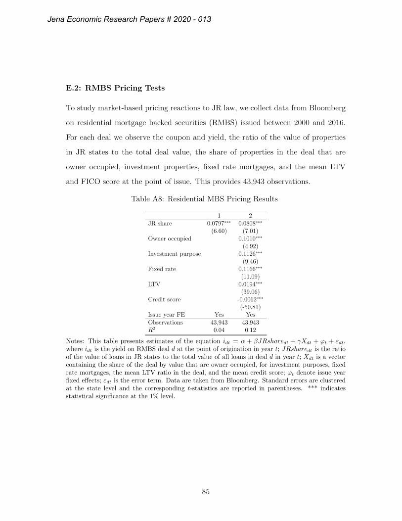
E.2: RMBS Pricing Tests
To study market-based pricing reactions to JR law, we collect data from Bloomberg
on residential mortgage backed securities (RMBS) issued between 2000 and 2016.
For each deal we observe the coupon and yield, the ratio of the value of properties
in JR states to the total deal value, the share of properties in the deal that are
owner occupied, investment properties, fixed rate mortgages, and the mean LTV
and FICO score at the point of issue. This provides 43,943 observations.
Table A8: Residential MBS Pricing Results
1 2JR share 0.0797∗∗∗ 0.0808∗∗∗
(6.60) (7.01)Owner occupied 0.1010∗∗∗
(4.92)Investment purpose 0.1126∗∗∗
(9.46)Fixed rate 0.1166∗∗∗
(11.09)LTV 0.0194∗∗∗
(39.06)Credit score -0.0062∗∗∗
(-50.81)Issue year FE Yes YesObservations 43,943 43,943R2 0.04 0.12
Notes: This table presents estimates of the equation idt = α + βJRsharedt + γXdt + ϕt + εdt,where idt is the yield on RMBS deal d at the point of origination in year t; JRsharedt is the ratioof the value of loans in JR states to the total value of all loans in deal d in year t; Xdt is a vectorcontaining the share of the deal by value that are owner occupied, for investment purposes, fixedrate mortgages, the mean LTV ratio in the deal, and the mean credit score; ϕt denote issue yearfixed effects; εdt is the error term. Data are taken from Bloomberg. Standard errors are clusteredat the state level and the corresponding t-statistics are reported in parentheses. *** indicatesstatistical significance at the 1% level.
85
Jena Economic Research Papers # 2020 - 013
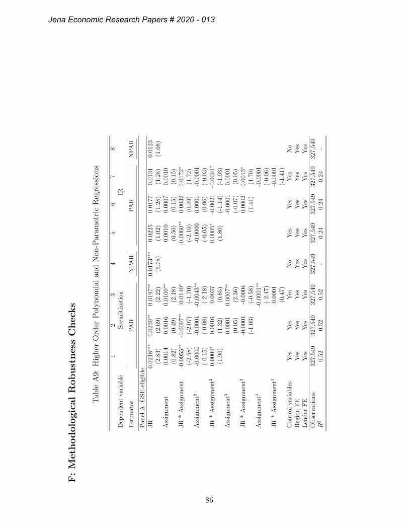
F:
Meth
od
olo
gic
al
Rob
ust
ness
Ch
eck
s
Tab
leA
9:H
igher
Ord
erP
olynom
ial
and
Non
-Par
amet
ric
Reg
ress
ions
12
34
56
78
Dep
enden
tva
riab
leSec
uri
tiza
tion
IR
Est
imat
orP
AR
NP
AR
PA
RN
PA
R
Pan
elA
:G
SE
-eligi
ble
JR
0.02
18∗∗
∗0.
0239
∗∗0.
0197
∗∗0.
0173
∗∗∗
0.02
250.
0177
0.01
310.
0123
(2.8
3)(2
.69)
(2.2
2)(5
.78)
(1.0
2)(1
.28)
(1.2
8)(1
.08)
Ass
ignm
ent
0.00
140.
0016
0.01
00∗∗
0.00
100.
0007
0.00
10(0
.82)
(0.4
9)(2
.18)
(0.5
0)(0
.15)
(0.1
5)JR
*A
ssig
nm
ent
-0.0
055∗
∗-0
.009
7∗∗
-0.0
140∗
-0.0
060∗
∗0.
0032
0.01
72∗
(-2.
58)
(-2.
07)
(-1.
70)
(-2.
10)
(0.4
9)(1
.72)
Ass
ignm
ent2
-0.0
000
-0.0
001
-0.0
043∗
∗-0
.000
00.
0001
-0.0
001
(-0.
15)
(-0.
08)
(-2.
18)
(-0.
05)
(0.0
6)(-
0.03
)JR
*A
ssig
nm
ent2
0.00
04∗
0.00
160.
0037
0.00
05∗
-0.0
021
-0.0
091∗
(1.9
0)(1
.32)
(0.8
5)(1
.80)
(-1.
14)
(-1.
93)
Ass
ignm
ent3
0.00
010.
0007
∗∗-0
.000
10.
0001
(0.0
5)(2
.36)
(-0.
07)
(0.0
5)JR
*A
ssig
nm
ent3
-0.0
001
-0.0
004
0.00
020.
0013
∗
(-1.
03)
(-0.
58)
(1.4
1)(1
.70)
Ass
ignm
ent4
-0.0
001∗
∗-0
.000
1(-
2.47
)(-
0.06
)JR
*A
ssig
nm
ent4
0.00
01-0
.000
1(0
.47)
(-1.
41)
Con
trol
vari
able
sY
esY
esY
esN
oY
esY
esY
esN
oR
egio
nF
EY
esY
esY
esY
esY
esY
esY
esY
esL
ender
FE
Yes
Yes
Yes
Yes
Yes
Yes
Yes
Yes
Obse
rvat
ions
327,
549
327,
549
327,
549
327,
549
327,
549
327,
549
327,
549
327,
549
R2
0.52
0.52
0.52
-0.
240.
240.
24-
86
Jena Economic Research Papers # 2020 - 013
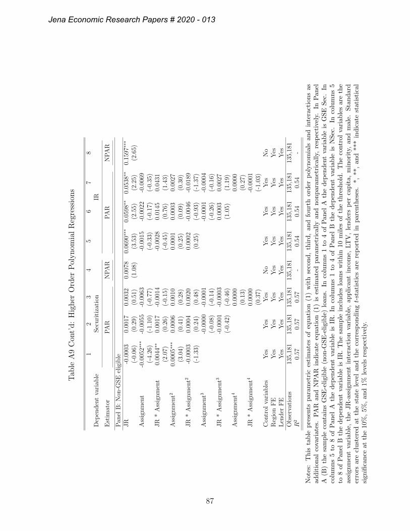
Tab
leA
9C
ont’
d:
Hig
her
Ord
erP
olynom
ial
Reg
ress
ions
12
34
56
78
Dep
enden
tva
riab
leSec
uri
tiza
tion
IR
Est
imat
orP
AR
NP
AR
PA
RN
PA
R
Pan
elB
:N
on-G
SE
elig
ible
JR
-0.0
003
0.00
170.
0032
0.00
780.
0690
∗∗∗
0.05
98∗∗
0.05
38∗∗
0.15
97∗∗
∗
(-0.
06)
(0.2
9)(0
.51)
(1.0
8)(3
.53)
(2.5
5)(2
.25)
(2.6
5)A
ssig
nm
ent
-0.0
052∗
∗∗-0
.005
5-0
.006
3-0
.001
5-0
.002
2-0
.006
9(-
4.26
)(-
1.10
)(-
0.77
)(-
0.33
)(-
0.17
)(-
0.35
)JR
*A
ssig
nm
ent
0.00
44∗∗
0.00
17-0
.001
4-0
.002
80.
0145
0.04
31(2
.07)
(0.2
6)(-
0.15
)(-
0.45
)(0
.76)
(1.4
3)A
ssig
nm
ent2
0.00
05∗∗
∗0.
0006
0.00
100.
0001
0.00
030.
0027
(3.0
4)(0
.41)
(0.2
8)(0
.25)
(0.0
9)(0
.30)
JR
*A
ssig
nm
ent2
-0.0
003
0.00
040.
0020
0.00
02-0
.004
6-0
.018
9(-
1.33
)(0
.24)
(0.4
8)(0
.25)
(-0.
93)
(-1.
37)
Ass
ignm
ent3
-0.0
000
-0.0
001
-0.0
001
-0.0
004
(-0.
08)
(-0.
14)
(-0.
26)
(-0.
16)
JR
*A
ssig
nm
ent3
-0.0
001
-0.0
003
0.00
030.
0027
(-0.
42)
(-0.
46)
(1.0
5)(1
.19)
Ass
ignm
ent4
0.00
000.
0000
(0.1
3)(0
.27)
JR
*A
ssig
nm
ent4
0.00
00-0
.000
1(0
.37)
(-1.
03)
Con
trol
vari
able
sY
esY
esY
esN
oY
esY
esY
esN
oR
egio
nF
EY
esY
esY
esY
esY
esY
esY
esY
esL
ender
FE
Yes
Yes
Yes
Yes
Yes
Yes
Yes
Yes
Obse
rvat
ions
135,
181
135,
181
135,
181
135,
181
135,
181
135,
181
135,
181
135,
181
R2
0.57
0.57
0.57
-0.
540.
540.
54-
Not
es:
Th
ista
ble
pre
sents
par
am
etri
ces
tim
ate
sof
equat
ion
(1)
wit
hse
con
d,
thir
d,
and
fou
rth
ord
erp
olyn
omia
lsan
din
tera
ctio
ns
asad
dit
ion
alco
vari
ates
.P
AR
an
dN
PA
Rin
dic
ate
equ
atio
n(1
)is
esti
mat
edp
aram
etri
call
yan
dn
onp
aram
etri
call
y,re
spec
tivel
y.In
Pan
elA
(B)
the
sam
ple
conta
ins
GS
E-e
ligib
le(n
on-G
SE
-eli
gib
le)
loan
s.In
colu
mn
s1
to4
ofP
anel
Ath
ed
epen
den
tva
riab
leis
GS
ES
ec.
Inco
lum
ns
5to
8of
Pan
elA
the
dep
end
ent
vari
able
isIR
.In
colu
mn
s1
to4
ofP
anel
Bth
ed
epen
den
tva
riab
leis
NS
ec.
Inco
lum
ns
5to
8of
Pan
elB
the
dep
end
ent
vari
able
isIR
.T
he
sam
ple
incl
ud
eslo
ans
wit
hin
10m
iles
ofth
eth
resh
old
.T
he
contr
olva
riab
les
are
the
assi
gnm
ent
vari
able
,th
eJR
-ass
ign
men
tin
tera
ctio
nva
riab
le,
app
lica
nt
inco
me,
LT
V,
len
der
sp
erca
pit
a,m
inor
ity,
and
mal
e.S
tan
dar
der
rors
are
clu
ster
edat
the
stat
ele
vel
and
the
corr
esp
ond
ingt-
stat
isti
csar
ere
por
ted
inp
aren
thes
es.
*,**
,an
d**
*in
dic
ate
stat
isti
cal
sign
ifica
nce
atth
e10
%,
5%,
and
1%le
vel
sre
spec
tive
ly.
87
Jena Economic Research Papers # 2020 - 013
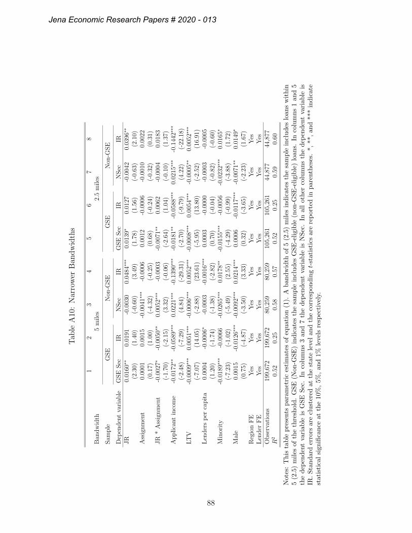
Tab
leA
10:
Nar
row
erB
andw
idth
s
12
34
56
78
Ban
dw
idth
5m
iles
2.5
miles
Sam
ple
GSE
Non
-GSE
GSE
Non
-GSE
Dep
enden
tva
riab
leG
SE
Sec
IRN
Sec
IRG
SE
Sec
IRN
Sec
IRJR
0.01
60∗∗
0.01
91-0
.003
00.
0484
∗∗∗
0.01
39∗
0.01
27-0
.004
20.
0396
∗∗
(2.3
0)(1
.40)
(-0.
60)
(3.4
9)(1
.78)
(1.5
6)(-
0.63
)(2
.10)
Ass
ignm
ent
0.00
010.
0015
-0.0
041∗
∗∗-0
.000
60.
0012
-0.0
006
-0.0
010
0.00
22(0
.17)
(1.0
0)(-
4.32
)(-
0.25
)(0
.68)
(-0.
24)
(-0.
32)
(0.3
1)JR
*A
ssig
nm
ent
-0.0
027∗
-0.0
050∗
∗0.
0052
∗∗∗
-0.0
003
-0.0
071∗
∗0.
0062
-0.0
004
0.01
83(-
1.70
)(-
2.15
)(3
.32)
(-0.
06)
(-2.
64)
(1.0
4)(-
0.10
)(1
.37)
Applica
nt
inco
me
-0.0
172∗
∗-0
.058
9∗∗∗
0.02
21∗∗
∗-0
.139
0∗∗∗
-0.0
181∗
∗-0
.058
8∗∗∗
0.02
15∗∗
∗-0
.144
2∗∗∗
(-2.
48)
(-7.
29)
(4.8
4)(-
29.3
1)(-
2.70
)(-
9.79
)(4
.22)
(-22
.18)
LT
V-0
.000
9∗∗∗
0.00
51∗∗
∗-0
.000
6∗∗∗
0.00
52∗∗
∗-0
.000
8∗∗∗
0.00
54∗∗
∗-0
.000
5∗∗
0.00
52∗∗
∗
(-7.
07)
(14.
05)
(-2.
88)
(23.
61)
(-5.
95)
(13.
80)
(-2.
52)
(16.
91)
Len
der
sp
erca
pit
a0.
0004
-0.0
006∗
-0.0
003
-0.0
016∗
∗∗0.
0003
-0.0
000
-0.0
003
-0.0
005
(1.2
0)(-
1.74
)(-
1.38
)(-
2.82
)(0
.70)
(-0.
04)
(-0.
82)
(-0.
60)
Min
orit
y-0
.018
9∗∗∗
-0.0
066
-0.0
265∗
∗∗0.
0178
∗∗-0
.015
5∗∗∗
-0.0
056
-0.0
232∗
∗∗0.
0165
∗
(-7.
23)
(-1.
02)
(-5.
49)
(2.5
5)(-
4.29
)(-
0.99
)(-
3.88
)(1
.72)
Mal
e0.
0015
-0.0
126∗
∗∗-0
.009
2∗∗∗
0.02
14∗∗
∗0.
0006
-0.0
117∗
∗∗-0
.007
1∗∗
0.01
49∗
(0.7
5)(-
4.87
)(-
3.50
)(3
.33)
(0.3
2)(-
3.65
)(-
2.23
)(1
.67)
Reg
ion
FE
Yes
Yes
Yes
Yes
Yes
Yes
Yes
Yes
Len
der
FE
Yes
Yes
Yes
Yes
Yes
Yes
Yes
Yes
Obse
rvat
ions
199,
672
199,
672
80,2
5980
,259
105,
261
105,
261
44,8
7744
,877
R2
0.52
0.25
0.58
0.57
0.52
0.25
0.59
0.60
Not
es:
Th
ista
ble
pre
sents
par
amet
ric
esti
mat
esof
equ
atio
n(1
).A
ban
dw
idth
of5
(2.5
)m
iles
ind
icat
esth
esa
mp
lein
clu
des
loan
sw
ithin
5(2
.5)
mil
esof
the
thre
shold
.G
SE
(Non
-GS
E)
ind
icat
esth
esa
mp
lein
clu
des
GS
E-e
ligi
ble
(non
-GS
E-e
ligi
ble
)lo
ans.
Inco
lum
ns
1an
d5
the
dep
end
ent
vari
able
isG
SE
Sec
.In
colu
mn
s3
and
7th
ed
epen
den
tva
riab
leis
NS
ec.
Inal
lot
her
colu
mn
sth
ed
epen
den
tva
riab
leis
IR.
Sta
nd
ard
erro
rsar
ecl
ust
ered
atth
est
ate
leve
lan
dth
eco
rres
pon
din
gt-
stat
isti
csar
ere
por
ted
inp
aren
thes
es.
*,**
,an
d**
*in
dic
ate
stat
isti
cal
sign
ifica
nce
at
the
10%
,5%
,an
d1%
leve
lsre
spec
tive
ly.
88
Jena Economic Research Papers # 2020 - 013
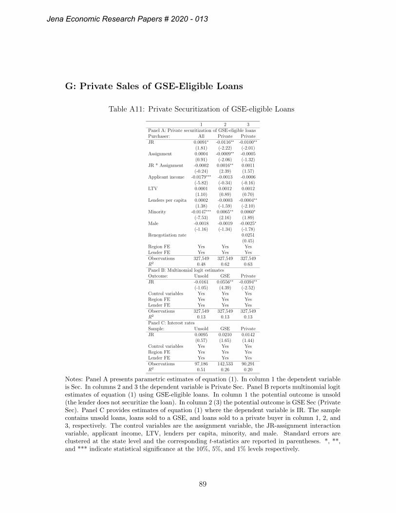
G: Private Sales of GSE-Eligible Loans
Table A11: Private Securitization of GSE-eligible Loans
1 2 3Panel A: Private securitization of GSE-eligible loansPurchaser: All Private PrivateJR 0.0091∗ -0.0116∗∗ -0.0100∗∗
(1.81) (-2.22) (-2.01)Assignment 0.0004 -0.0009∗∗ -0.0005
(0.91) (-2.06) (-1.32)JR * Assignment -0.0002 0.0016∗∗ 0.0011
(-0.24) (2.39) (1.57)Applicant income -0.0179∗∗∗ -0.0013 -0.0006
(-5.82) (-0.34) (-0.16)LTV 0.0001 0.0012 0.0012
(1.10) (0.89) (0.70)Lenders per capita 0.0002 -0.0003 -0.0004∗∗
(1.38) (-1.59) (-2.10)Minority -0.0147∗∗∗ 0.0065∗∗ 0.0060∗
(-7.53) (2.16) (1.89)Male -0.0018 -0.0019 -0.0025∗
(-1.16) (-1.34) (-1.78)Renegotiation rate 0.0251
(0.45)Region FE Yes Yes YesLender FE Yes Yes YesObservations 327,549 327,549 327,549R2 0.48 0.62 0.63Panel B: Multinomial logit estimatesOutcome: Unsold GSE PrivateJR -0.0161 0.0556∗∗ -0.0394∗∗
(-1.05) (4.39) (-2.52)Control variables Yes Yes YesRegion FE Yes Yes YesLender FE Yes Yes YesObservations 327,549 327,549 327,549R2 0.13 0.13 0.13Panel C: Interest ratesSample: Unsold GSE PrivateJR 0.0095 0.0210 0.0142
(0.57) (1.65) (1.44)Control variables Yes Yes YesRegion FE Yes Yes YesLender FE Yes Yes YesObservations 97,186 142,533 90,291R2 0.51 0.26 0.20
Notes: Panel A presents parametric estimates of equation (1). In column 1 the dependent variableis Sec. In columns 2 and 3 the dependent variable is Private Sec. Panel B reports multinomial logitestimates of equation (1) using GSE-eligible loans. In column 1 the potential outcome is unsold(the lender does not securitize the loan). In column 2 (3) the potential outcome is GSE Sec (PrivateSec). Panel C provides estimates of equation (1) where the dependent variable is IR. The samplecontains unsold loans, loans sold to a GSE, and loans sold to a private buyer in column 1, 2, and3, respectively. The control variables are the assignment variable, the JR-assignment interactionvariable, applicant income, LTV, lenders per capita, minority, and male. Standard errors areclustered at the state level and the corresponding t-statistics are reported in parentheses. *, **,and *** indicate statistical significance at the 10%, 5%, and 1% levels respectively.
89
Jena Economic Research Papers # 2020 - 013
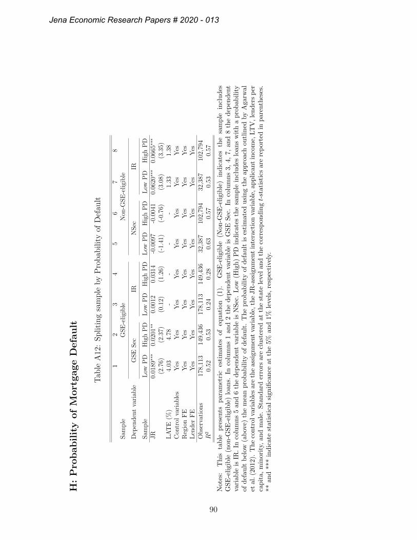
H:
Pro
bab
ilit
yof
Mort
gage
Defa
ult
Tab
leA
12:
Spliti
ng
sam
ple
by
Pro
bab
ilit
yof
Def
ault
12
34
56
78
Sam
ple
GSE
-eligi
ble
Non
-GSE
-eligi
ble
Dep
enden
tva
riab
leG
SE
Sec
IRN
Sec
IR
Sam
ple
Low
PD
Hig
hP
DL
owP
DH
igh
PD
Low
PD
Hig
hP
DL
owP
DH
igh
PD
JR
0.01
89∗∗
∗0.
0201
∗∗0.
0012
0.03
14-0
.009
7-0
.004
10.
0620
∗∗∗
0.06
65∗∗
∗
(2.7
6)(2
.37)
(0.1
2)(1
.26)
(-1.
41)
(-0.
76)
(3.0
8)(3
.35)
LA
TE
(%)
4.03
4.78
--
--
1.33
1.38
Con
trol
vari
able
sY
esY
esY
esY
esY
esY
esY
esY
esR
egio
nF
EY
esY
esY
esY
esY
esY
esY
esY
esL
ender
FE
Yes
Yes
Yes
Yes
Yes
Yes
Yes
Yes
Obse
rvat
ions
178,
113
149,
436
178,
113
149,
436
32,3
8710
2,79
432
,387
102,
794
R2
0.52
0.53
0.24
0.28
0.63
0.57
0.53
0.57
Not
es:
Th
ista
ble
pre
sents
par
amet
ric
esti
mat
esof
equ
atio
n(1
).G
SE
-eli
gib
le(N
on-G
SE
-eli
gib
le)
ind
icat
esth
esa
mp
lein
clu
des
GS
E-e
ligi
ble
(non
-GS
E-e
ligi
ble
)lo
ans.
Inco
lum
ns
1an
d2
the
dep
end
ent
vari
able
isG
SE
Sec
.In
colu
mn
s3,
4,7,
and
8th
ed
epen
den
tva
riab
leis
IR.
Inco
lum
ns
5an
d6
the
dep
end
ent
vari
able
isN
Sec
.L
ow(H
igh)
PD
indic
ates
the
sam
ple
incl
ud
eslo
ans
wit
ha
pro
bab
ilit
yof
def
ault
bel
ow(a
bov
e)th
em
ean
pro
bab
ilit
yof
def
ault
.T
he
pro
bab
ilit
yof
def
ault
ises
tim
ated
usi
ng
the
app
roac
hou
tlin
edby
Aga
rwal
etal
.(2
012)
.T
he
contr
olva
riab
les
are
the
assi
gnm
ent
vari
able
,th
eJR
-ass
ign
men
tin
tera
ctio
nva
riab
le,ap
pli
cant
inco
me,
LT
V,le
nd
ers
per
cap
ita,
min
orit
y,an
dm
ale.
Sta
nd
ard
erro
rsar
ecl
ust
ered
atth
est
ate
leve
lan
dth
eco
rres
pon
din
gt-
stat
isti
csar
ere
por
ted
inp
aren
thes
es.
**an
d**
*in
dic
ate
stat
isti
cal
sign
ifica
nce
at
the
5%an
d1%
leve
ls,
resp
ecti
vely
.
90
Jena Economic Research Papers # 2020 - 013
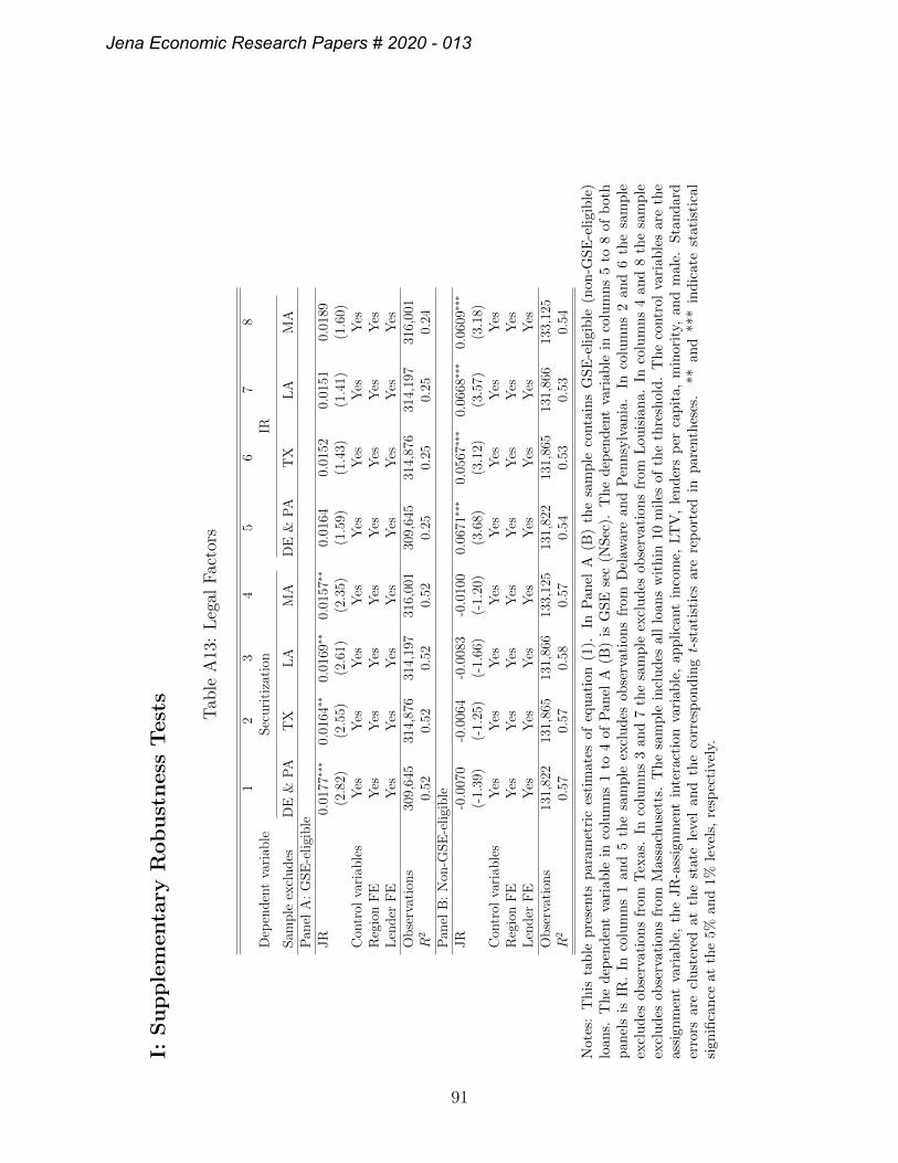
I:S
up
ple
menta
ryR
ob
ust
ness
Test
s
Tab
leA
13:
Leg
alF
acto
rs
12
34
56
78
Dep
enden
tva
riab
leSec
uri
tiza
tion
IR
Sam
ple
excl
udes
DE
&P
AT
XL
AM
AD
E&
PA
TX
LA
MA
Pan
elA
:G
SE
-eligi
ble
JR
0.01
77∗∗
∗0.
0164
∗∗0.
0169
∗∗0.
0157
∗∗0.
0164
0.01
520.
0151
0.01
89(2
.82)
(2.5
5)(2
.61)
(2.3
5)(1
.59)
(1.4
3)(1
.41)
(1.6
0)C
ontr
olva
riab
les
Yes
Yes
Yes
Yes
Yes
Yes
Yes
Yes
Reg
ion
FE
Yes
Yes
Yes
Yes
Yes
Yes
Yes
Yes
Len
der
FE
Yes
Yes
Yes
Yes
Yes
Yes
Yes
Yes
Obse
rvat
ions
309,
645
314,
876
314,
197
316,
001
309,
645
314,
876
314,
197
316,
001
R2
0.52
0.52
0.52
0.52
0.25
0.25
0.25
0.24
Pan
elB
:N
on-G
SE
-eligi
ble
JR
-0.0
070
-0.0
064
-0.0
083
-0.0
100
0.06
71∗∗
∗0.
0567
∗∗∗
0.06
68∗∗
∗0.
0609
∗∗∗
(-1.
39)
(-1.
25)
(-1.
66)
(-1.
20)
(3.6
8)(3
.12)
(3.5
7)(3
.18)
Con
trol
vari
able
sY
esY
esY
esY
esY
esY
esY
esY
esR
egio
nF
EY
esY
esY
esY
esY
esY
esY
esY
esL
ender
FE
Yes
Yes
Yes
Yes
Yes
Yes
Yes
Yes
Obse
rvat
ions
131,
822
131,
865
131,
866
133,
125
131,
822
131,
865
131,
866
133,
125
R2
0.57
0.57
0.58
0.57
0.54
0.53
0.53
0.54
Not
es:
Th
ista
ble
pre
sents
par
am
etri
ces
tim
ates
ofeq
uat
ion
(1).
InP
anel
A(B
)th
esa
mp
leco
nta
ins
GS
E-e
ligi
ble
(non
-GS
E-e
ligi
ble
)lo
ans.
Th
ed
epen
den
tva
riab
lein
colu
mn
s1
to4
ofP
anel
A(B
)is
GS
Ese
c(N
Sec
).T
he
dep
end
ent
vari
able
inco
lum
ns
5to
8of
bot
hp
anel
sis
IR.
Inco
lum
ns
1an
d5
the
sam
ple
excl
ud
esob
serv
atio
ns
from
Del
awar
ean
dP
enn
sylv
ania
.In
colu
mn
s2
and
6th
esa
mp
leex
clu
des
obse
rvat
ion
sfr
omT
exas
.In
colu
mn
s3
and
7th
esa
mp
leex
clu
des
obse
rvat
ion
sfr
omL
ouis
ian
a.In
colu
mn
s4
and
8th
esa
mp
leex
clu
des
obse
rvat
ion
sfr
omM
assa
chu
sett
s.T
he
sam
ple
incl
ud
esal
llo
ans
wit
hin
10m
iles
ofth
eth
resh
old
.T
he
contr
olva
riab
les
are
the
assi
gnm
ent
vari
able
,th
eJR
-ass
ign
men
tin
tera
ctio
nva
riab
le,
app
lica
nt
inco
me,
LT
V,
len
der
sp
erca
pit
a,m
inor
ity,
and
mal
e.S
tan
dar
der
rors
are
clu
ster
edat
the
state
leve
lan
dth
eco
rres
pon
din
gt-
stat
isti
csar
ere
por
ted
inp
aren
thes
es.
**an
d**
*in
dic
ate
stat
isti
cal
sign
ifica
nce
atth
e5%
and
1%le
vels
,re
spec
tive
ly.
91
Jena Economic Research Papers # 2020 - 013
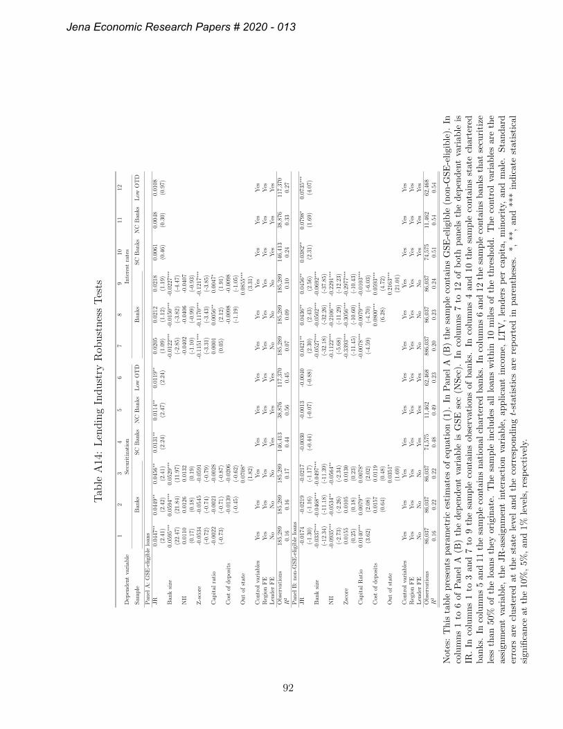
Tab
leA
14:
Len
din
gIn
dust
ryR
obust
nes
sT
ests
12
34
56
78
910
1112
Dep
enden
tva
riab
leSec
uri
tiza
tion
Inte
rest
rate
s
Sam
ple
Ban
ks
SC
Ban
ks
NC
Ban
ks
Low
OT
DB
anks
SC
Ban
ks
NC
Ban
ks
Low
OT
D
Pan
elA
:G
SE
-eligi
ble
loan
sJR
0.04
47∗∗
0.04
49∗∗
0.04
56∗∗
0.01
31∗∗
0.01
14∗∗
0.01
19∗∗
0.02
050.
0212
0.02
180.
0061
0.00
480.
0108
(2.4
1)(2
.42)
(2.4
1)(2
.24)
(2.4
7)(2
.24)
(1.0
9)(1
.12)
(1.1
9)(0
.46)
(0.3
0)(0
.97)
Ban
ksi
ze0.
0595
∗∗∗
0.05
94∗∗
∗0.
0529
∗∗∗
-0.0
122∗
∗∗-0
.015
0∗∗∗
-0.0
227∗
∗∗
(22.
47)
(21.
84)
(11.
97)
(-2.
85)
(-3.
82)
(-4.
47)
NII
0.01
100.
0126
0.01
32-0
.040
2-0
.040
6-0
.040
7(0
.17)
(0.1
8)(0
.19)
(-1.
10)
(-0.
99)
(-0.
93)
Z-s
core
-0.0
534
-0.0
545
-0.0
591
-0.1
151∗
∗∗-0
.117
0∗∗∗
-0.1
217∗
∗∗
(-0.
72)
(-0.
74)
(-0.
79)
(-3.
31)
(-3.
43)
(-3.
85)
Cap
ital
rati
o-0
.002
2-0
.002
1-0
.002
80.
0001
0.00
56∗∗
0.00
47∗
(-0.
73)
(-0.
71)
(-0.
87)
(0.0
5)(2
.12)
(1.9
1)C
ost
ofdep
osit
s-0
.013
9-0
.020
6-0
.009
8-0
.009
8(-
0.45
)(-
0.62
)(-
1.19
)(-
1.05
)O
ut
ofst
ate
0.07
08∗
0.08
55∗∗
∗
(1.8
2)(3
.31)
Con
trol
vari
able
sY
esY
esY
esY
esY
esY
esY
esY
esY
esY
esY
esY
esR
egio
nF
EY
esY
esY
esY
esY
esY
esY
esY
esY
esY
esY
esY
esL
ender
FE
No
No
No
Yes
Yes
Yes
No
No
No
Yes
Yes
Yes
Obse
rvat
ions
185,
289
185,
289
185,
289
146,
413
38,8
7611
7,37
018
5,28
918
5,28
918
5,28
914
6,41
338
,876
117,
370
R2
0.16
0.16
0.17
0.44
0.56
0.45
0.07
0.09
0.10
0.24
0.33
0.27
Pan
elB
:non
-GSE
-eligi
ble
loan
sJR
-0.0
174
-0.0
219
-0.0
217
-0.0
030
-0.0
013
-0.0
040
0.04
21∗∗
0.04
36∗∗
0.04
56∗∗
0.03
82∗∗
0.07
98∗
0.07
35∗∗
∗
(-1.
30)
(-1.
16)
(-1.
17)
(-0.
44)
(-0.
07)
(-0.
88)
(2.3
0)(2
.43)
(2.5
6)(2
.31)
(1.6
9)(4
.07)
Ban
ksi
ze-0
.033
7∗∗∗
-0.0
468∗
∗∗-0
.049
7∗∗∗
-0.0
527∗
∗∗-0
.050
2∗∗∗
-0.0
692∗
∗∗
(-12
.34)
(-11
.18)
(-11
.39)
(-32
.18)
(-32
.26)
(-37
.85)
NII
-0.0
935∗
∗∗-0
.053
4∗∗
-0.0
564∗
∗-0
.112
2∗∗∗
-0.2
106∗
∗∗-0
.229
1∗∗∗
(-2.
73)
(-2.
26)
(-2.
34)
(-5.
68)
(-11
.29)
(-12
.23)
Zsc
ore
0.01
550.
0105
0.01
30-0
.339
3∗∗∗
-0.3
056∗
∗∗-0
.297
7∗∗∗
(0.2
5)(0
.18)
(0.2
3)(-
11.4
5)(-
10.6
0)(-
10.4
3)C
apit
alR
atio
0.01
40∗∗
∗0.
0079
∗∗0.
0078
∗-0
.007
8∗∗∗
-0.0
079∗
∗∗-0
.010
3∗∗∗
(3.6
2)(2
.08)
(2.0
2)(-
4.59
)(-
4.70
)(-
6.03
)C
ost
ofdep
osit
s0.
0157
0.01
190.
0800
∗∗∗
0.05
93∗∗
∗
(0.6
4)(0
.48)
(6.2
8)(4
.72)
Out
ofst
ate
0.03
51∗
0.21
63∗∗
∗
(1.6
9)(2
1.01
)C
ontr
olva
riab
les
Yes
Yes
Yes
Yes
Yes
Yes
Yes
Yes
Yes
Yes
Yes
Yes
Reg
ion
FE
Yes
Yes
Yes
Yes
Yes
Yes
Yes
Yes
Yes
Yes
Yes
Yes
Len
der
FE
No
No
No
Yes
Yes
Yes
No
No
No
Yes
Yes
Yes
Obse
rvat
ions
86,0
3786
,037
86,0
3774
,575
11,4
6262
,468
886,
037
86,0
3786
,037
74,5
7511
,462
62,4
68R
20.
160.
220.
220.
480.
490.
230.
200.
230.
240.
510.
540.
54
Not
es:
Th
ista
ble
pre
sents
par
amet
ric
esti
mat
esof
equ
atio
n(1
).In
Pan
elA
(B)
the
sam
ple
conta
ins
GS
E-e
ligi
ble
(non
-GS
E-e
ligi
ble
).In
colu
mn
s1
to6
ofP
anel
A(B
)th
ed
epen
den
tva
riab
leis
GS
Ese
c(N
Sec
).In
colu
mn
s7
to12
ofb
oth
pan
els
the
dep
end
ent
vari
able
isIR
.In
colu
mn
s1
to3
and
7to
9th
esa
mp
leco
nta
ins
obse
rvat
ion
sof
ban
ks.
Inco
lum
ns
4an
d10
the
sam
ple
conta
ins
stat
ech
arte
red
ban
ks.
Inco
lum
ns
5an
d11
the
sam
ple
conta
ins
nat
ional
char
tere
db
anks.
Inco
lum
ns
6an
d12
the
sam
ple
conta
ins
ban
ks
that
secu
riti
zele
ssth
an50
%of
the
loan
sth
eyor
igin
ate.
Th
esa
mp
lein
clu
des
all
loan
sw
ith
in10
mil
esof
the
thre
shol
d.
Th
eco
ntr
olva
riab
les
are
the
assi
gnm
ent
vari
able
,th
eJR
-ass
ign
men
tin
tera
ctio
nva
riab
le,
app
lica
nt
inco
me,
LT
V,
len
der
sp
erca
pit
a,m
inor
ity,
and
mal
e.S
tan
dar
der
rors
are
clu
ster
edat
the
stat
ele
vel
and
the
corr
esp
ond
ingt-
stat
isti
csar
ere
por
ted
inp
aren
thes
es.
*,**
,an
d**
*in
dic
ate
stat
isti
cal
sign
ifica
nce
atth
e10
%,
5%,
and
1%le
vel
s,re
spec
tive
ly.
92
Jena Economic Research Papers # 2020 - 013
A danger is that there exist discontinuities in the incentive to default on other types
of debt at the threshold such that the estimates simply capture the riskiness of the
population that live in border areas. Although this appears implausible, we append
the empirical model with controls for the delinquency rate on automobile and credit
card debt. The effect of JR law in columns 1 and 2 of Table A15 remains robust.
The longer timeline in JR states may allow delinquent borrowers to self-cure.
Alternatively, the propensity to securitize a loan may differ across states because
the likelihood of successfully renegotiating with borrowers that default is lower due
to the longer foreclosure timeline in JR states (Piskorski et al., 2010; Agarwal et al.,
2011). The estimates in column 3 of Table A15 show that renegotiation does not
drive our inferences.
Lenders’ profitability expectations are also influenced by pre-payment risk. We
approximate pre-payment risk using the refinancing rate reported in HMDA on
mortgages over the past five years in each state. The results in column 4 of Table
A14 are similar to before. In column 5 of Table A15 we control for whether a
mortgage is an adjustable rate loan. This has no bearing on our findings. Han
et al. (2015) show that taxation is linked to securitization incentives. The results in
columns 6 and 7 of Table A15 demonstrate that the LATE is robust to controlling
for state-level corporate and personal tax rates.
93
Jena Economic Research Papers # 2020 - 013
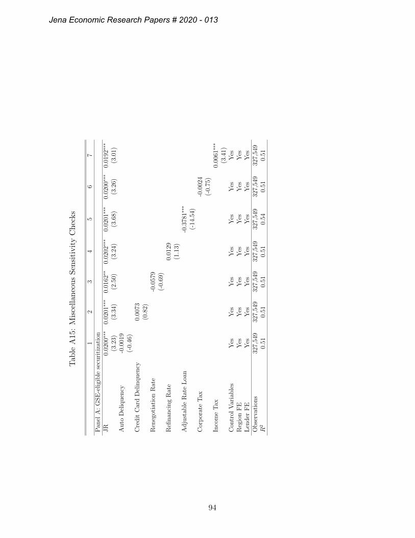
Tab
leA
15:
Mis
cellan
eous
Sen
siti
vit
yC
hec
ks
12
34
56
7P
anel
A:
GSE
-eligi
ble
secu
riti
zati
onJR
0.02
00∗∗
∗0.
0201
∗∗∗
0.01
62∗∗
0.02
02∗∗
∗0.
0201
∗∗∗
0.02
00∗∗
∗0.
0192
∗∗∗
(3.2
3)(3
.34)
(2.5
0)(3
.24)
(3.6
8)(3
.26)
(3.0
1)A
uto
Del
iquen
cy-0
.001
9(-
0.46
)C
redit
Car
dD
elin
quen
cy0.
0073
(0.8
2)R
eneg
otia
tion
Rat
e-0
.057
9(-
0.69
)R
efinan
cing
Rat
e0.
0129
(1.1
3)A
dju
stab
leR
ate
Loa
n-0
.378
1∗∗∗
(-14
.54)
Cor
por
ate
Tax
-0.0
024
(-0.
75)
Inco
me
Tax
0.00
61∗∗
∗
(3.4
1)C
ontr
olV
aria
ble
sY
esY
esY
esY
esY
esY
esY
esR
egio
nF
EY
esY
esY
esY
esY
esY
esY
esL
ender
FE
Yes
Yes
Yes
Yes
Yes
Yes
Yes
Obse
rvat
ions
327,
549
327,
549
327,
549
327,
549
327,
549
327,
549
327,
549
R2
0.51
0.51
0.51
0.51
0.54
0.51
0.51
94
Jena Economic Research Papers # 2020 - 013
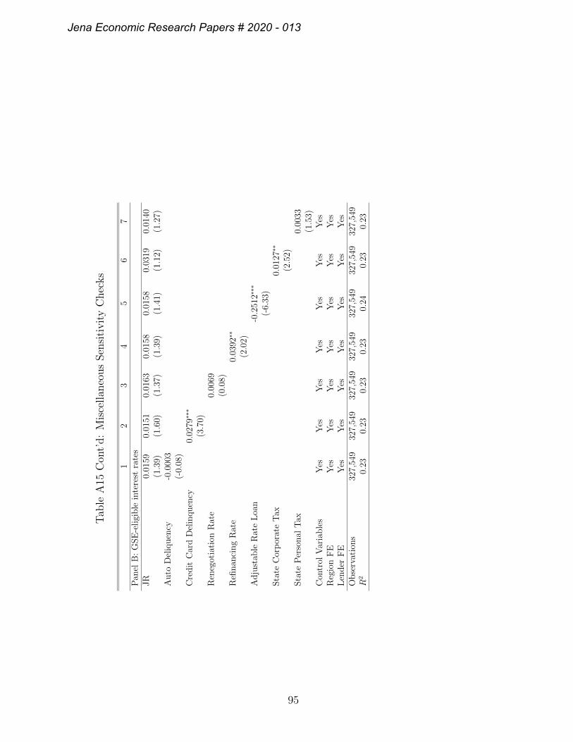
Tab
leA
15C
ont’
d:
Mis
cellan
eous
Sen
siti
vit
yC
hec
ks
12
34
56
7P
anel
B:
GSE
-eligi
ble
inte
rest
rate
sJR
0.01
590.
0151
0.01
630.
0158
0.01
580.
0319
0.01
40(1
.39)
(1.6
0)(1
.37)
(1.3
9)(1
.41)
(1.1
2)(1
.27)
Auto
Del
iquen
cy-0
.000
3(-
0.08
)C
redit
Car
dD
elin
quen
cy0.
0279
∗∗∗
(3.7
0)R
eneg
otia
tion
Rat
e0.
0069
(0.0
8)R
efinan
cing
Rat
e0.
0392
∗∗
(2.0
2)A
dju
stab
leR
ate
Loa
n-0
.251
2∗∗∗
(-6.
33)
Sta
teC
orp
orat
eT
ax0.
0127
∗∗
(2.5
2)Sta
teP
erso
nal
Tax
0.00
33(1
.53)
Con
trol
Var
iable
sY
esY
esY
esY
esY
esY
esY
esR
egio
nF
EY
esY
esY
esY
esY
esY
esY
esL
ender
FE
Yes
Yes
Yes
Yes
Yes
Yes
Yes
Obse
rvat
ions
327,
549
327,
549
327,
549
327,
549
327,
549
327,
549
327,
549
R2
0.23
0.23
0.23
0.23
0.24
0.23
0.23
95
Jena Economic Research Papers # 2020 - 013
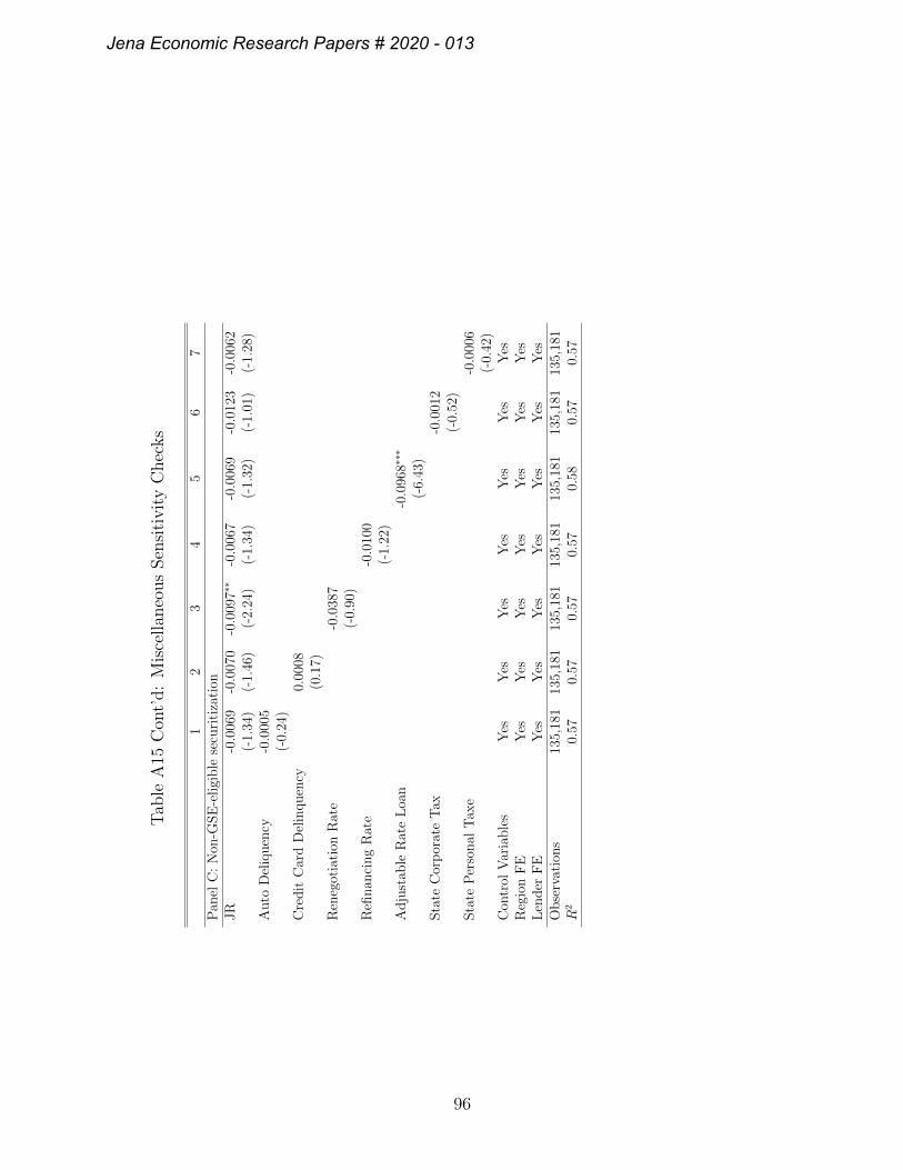
Tab
leA
15C
ont’
d:
Mis
cellan
eous
Sen
siti
vit
yC
hec
ks
12
34
56
7P
anel
C:
Non
-GSE
-eligi
ble
secu
riti
zati
onJR
-0.0
069
-0.0
070
-0.0
097∗
∗-0
.006
7-0
.006
9-0
.012
3-0
.006
2(-
1.34
)(-
1.46
)(-
2.24
)(-
1.34
)(-
1.32
)(-
1.01
)(-
1.28
)A
uto
Del
iquen
cy-0
.000
5(-
0.24
)C
redit
Car
dD
elin
quen
cy0.
0008
(0.1
7)R
eneg
otia
tion
Rat
e-0
.038
7(-
0.90
)R
efinan
cing
Rat
e-0
.010
0(-
1.22
)A
dju
stab
leR
ate
Loa
n-0
.096
8∗∗∗
(-6.
43)
Sta
teC
orp
orat
eT
ax-0
.001
2(-
0.52
)Sta
teP
erso
nal
Tax
e-0
.000
6(-
0.42
)C
ontr
olV
aria
ble
sY
esY
esY
esY
esY
esY
esY
esR
egio
nF
EY
esY
esY
esY
esY
esY
esY
esL
ender
FE
Yes
Yes
Yes
Yes
Yes
Yes
Yes
Obse
rvat
ions
135,
181
135,
181
135,
181
135,
181
135,
181
135,
181
135,
181
R2
0.57
0.57
0.57
0.57
0.58
0.57
0.57
96
Jena Economic Research Papers # 2020 - 013
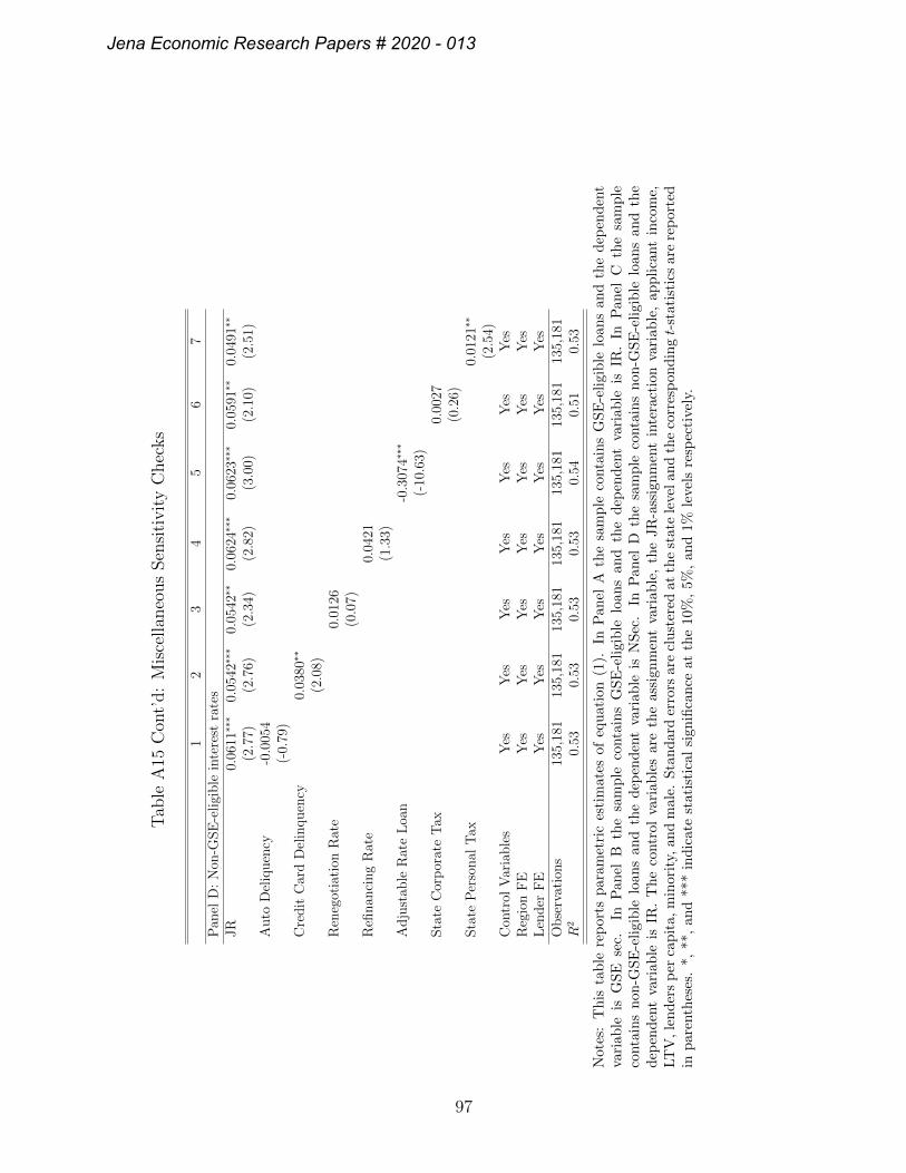
Tab
leA
15C
ont’
d:
Mis
cellan
eous
Sen
siti
vit
yC
hec
ks
12
34
56
7P
anel
D:
Non
-GSE
-eligi
ble
inte
rest
rate
sJR
0.06
11∗∗
∗0.
0542
∗∗∗
0.05
42∗∗
0.06
24∗∗
∗0.
0623
∗∗∗
0.05
91∗∗
0.04
91∗∗
(2.7
7)(2
.76)
(2.3
4)(2
.82)
(3.0
0)(2
.10)
(2.5
1)A
uto
Del
iquen
cy-0
.005
4(-
0.79
)C
redit
Car
dD
elin
quen
cy0.
0380
∗∗
(2.0
8)R
eneg
otia
tion
Rat
e0.
0126
(0.0
7)R
efinan
cing
Rat
e0.
0421
(1.3
3)A
dju
stab
leR
ate
Loa
n-0
.307
4∗∗∗
(-10
.63)
Sta
teC
orp
orat
eT
ax0.
0027
(0.2
6)Sta
teP
erso
nal
Tax
0.01
21∗∗
(2.5
4)C
ontr
olV
aria
ble
sY
esY
esY
esY
esY
esY
esY
esR
egio
nF
EY
esY
esY
esY
esY
esY
esY
esL
ender
FE
Yes
Yes
Yes
Yes
Yes
Yes
Yes
Obse
rvat
ions
135,
181
135,
181
135,
181
135,
181
135,
181
135,
181
135,
181
R2
0.53
0.53
0.53
0.53
0.54
0.51
0.53
Not
es:
Th
ista
ble
rep
orts
para
met
ric
esti
mate
sof
equ
atio
n(1
).In
Pan
elA
the
sam
ple
conta
ins
GSE
-eligi
ble
loan
san
dth
ed
epen
den
tva
riab
leis
GS
Ese
c.In
Pan
elB
the
sam
ple
conta
ins
GS
E-e
ligi
ble
loan
san
dth
ed
epen
den
tva
riab
leis
IR.
InP
anel
Cth
esa
mp
leco
nta
ins
non
-GS
E-e
ligi
ble
loan
san
dth
ed
epen
den
tva
riab
leis
NS
ec.
InP
anel
Dth
esa
mp
leco
nta
ins
non
-GS
E-e
ligi
ble
loan
san
dth
ed
epen
den
tva
riab
leis
IR.
Th
eco
ntr
olva
riab
les
are
the
assi
gnm
ent
vari
able
,th
eJR
-ass
ign
men
tin
tera
ctio
nva
riab
le,
app
lica
nt
inco
me,
LT
V,le
nd
ers
per
cap
ita,
min
orit
y,an
dm
ale.
Sta
nd
ard
erro
rsar
ecl
ust
ered
atth
est
ate
leve
lan
dth
eco
rres
pon
din
gt-
stat
isti
csar
ere
por
ted
inp
aren
thes
es.
*,**
,an
d**
*in
dic
ate
stat
isti
cal
sign
ifica
nce
atth
e10
%,
5%,
and
1%le
vel
sre
spec
tive
ly.
97
Jena Economic Research Papers # 2020 - 013
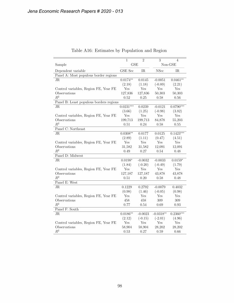
Table A16: Estimates by Population and Region
1 2 3 4Sample GSE Non-GSE
Dependent variable GSE Sec IR NSec IRPanel A: Most populous border regionsJR 0.0174∗∗ 0.0145 -0.0051 0.0461∗∗
(2.18) (1.18) (-0.89) (2.21)Control variables, Region FE, Year FE Yes Yes Yes YesObservations 127,836 127,836 50,303 50,303R2 0.52 0.25 0.58 0.56Panel B: Least populous borders regionsJR 0.0231∗∗∗ 0.0239 -0.0121 0.0790∗∗∗
(3.66) (1.25) (-0.98) (3.82)Control variables, Region FE, Year FE Yes Yes Yes YesObservations 199,713 199,713 84,878 55,203R2 0.51 0.24 0.58 0.55Panel C: NortheastJR 0.0308∗∗ 0.0177 0.0125 0.1423∗∗∗
(2.89) (1.11) (0.47) (4.51)Control variables, Region FE, Year FE Yes Yes Yes YesObservations 31,582 31,582 12,091 12,091R2 0.49 0.27 0.54 0.48Panel D: MidwestJR 0.0198∗ -0.0032 -0.0033 0.0159∗
(1.84) (-0.20) (-0.49) (1.79)Control variables, Region FE, Year FE Yes Yes Yes YesObservations 127,187 127,187 43,878 43,878R2 0.51 0.20 0.58 0.48Panel E: WestJR 0.1229 0.2792 -0.0079 0.4032
(0.98) (1.46) (-0.05) (0.98)Control variables, Region FE, Year FE Yes Yes Yes YesObservations 458 458 309 309R2 0.77 0.54 0.69 0.93Panel F: SouthJR 0.0186∗∗ -0.0023 -0.0318∗∗ 0.2360∗∗∗
(2.12) (-0.15) (-2.01) (4.96)Control variables, Region FE, Year FE Yes Yes Yes YesObservations 58,904 58,904 28,202 28,202R2 0.53 0.27 0.59 0.66
98
Jena Economic Research Papers # 2020 - 013
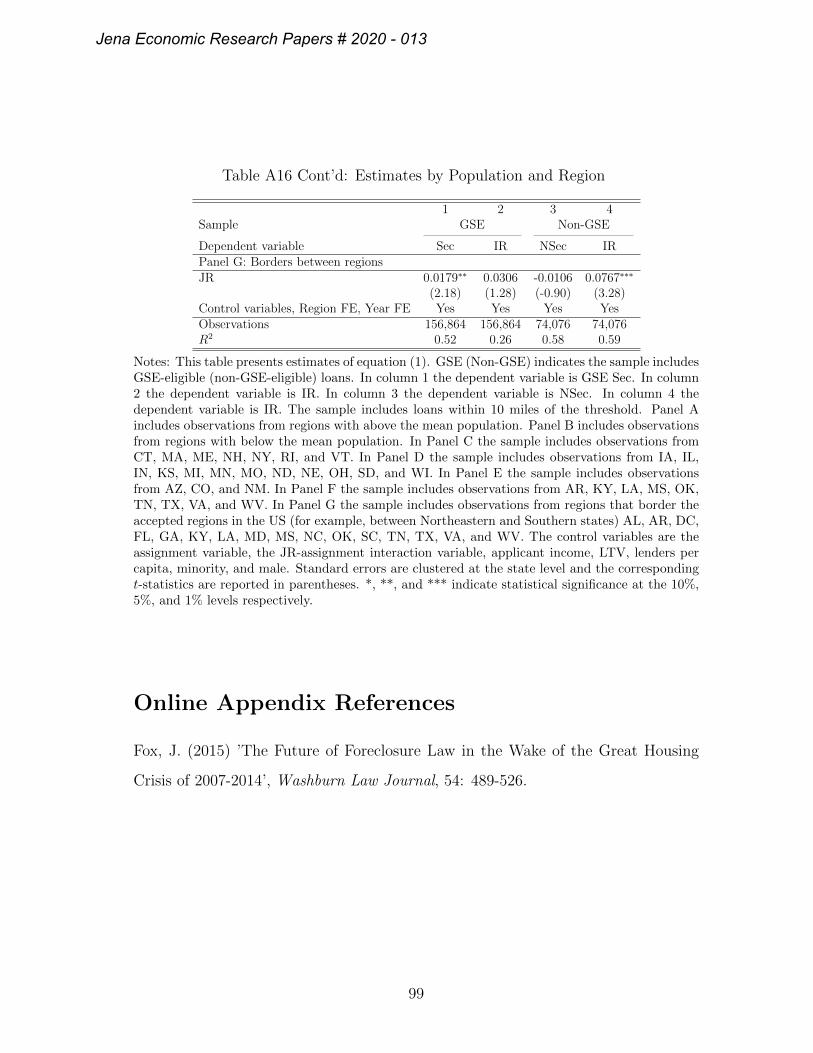
Table A16 Cont’d: Estimates by Population and Region
1 2 3 4Sample GSE Non-GSE
Dependent variable Sec IR NSec IRPanel G: Borders between regionsJR 0.0179∗∗ 0.0306 -0.0106 0.0767∗∗∗
(2.18) (1.28) (-0.90) (3.28)Control variables, Region FE, Year FE Yes Yes Yes YesObservations 156,864 156,864 74,076 74,076R2 0.52 0.26 0.58 0.59
Notes: This table presents estimates of equation (1). GSE (Non-GSE) indicates the sample includesGSE-eligible (non-GSE-eligible) loans. In column 1 the dependent variable is GSE Sec. In column2 the dependent variable is IR. In column 3 the dependent variable is NSec. In column 4 thedependent variable is IR. The sample includes loans within 10 miles of the threshold. Panel Aincludes observations from regions with above the mean population. Panel B includes observationsfrom regions with below the mean population. In Panel C the sample includes observations fromCT, MA, ME, NH, NY, RI, and VT. In Panel D the sample includes observations from IA, IL,IN, KS, MI, MN, MO, ND, NE, OH, SD, and WI. In Panel E the sample includes observationsfrom AZ, CO, and NM. In Panel F the sample includes observations from AR, KY, LA, MS, OK,TN, TX, VA, and WV. In Panel G the sample includes observations from regions that border theaccepted regions in the US (for example, between Northeastern and Southern states) AL, AR, DC,FL, GA, KY, LA, MD, MS, NC, OK, SC, TN, TX, VA, and WV. The control variables are theassignment variable, the JR-assignment interaction variable, applicant income, LTV, lenders percapita, minority, and male. Standard errors are clustered at the state level and the correspondingt-statistics are reported in parentheses. *, **, and *** indicate statistical significance at the 10%,5%, and 1% levels respectively.
Online Appendix References
Fox, J. (2015) ’The Future of Foreclosure Law in the Wake of the Great Housing
Crisis of 2007-2014’, Washburn Law Journal, 54: 489-526.
99
Jena Economic Research Papers # 2020 - 013

IMPRESSUM
Jena Economic Research Papers
ISSN 1864-7057
Friedrich Schiller University Jena
Faculty of Economics and Business Administration
Carl-Zeiss-Str. 3
D-07743 Jena, Germany
Email: [email protected]
Editor: Silke Übelmesser
Website: www.wiwi.uni-jena.de/en/jerp
© by the author
![Untitled Document []untitled document running back danny nephew 5'10" 210 mtn. view senior running back mike borden 6' 185 dobson senior wide receiver brendan mcgowan 6' 165 mtn. view](https://img.pdfslide.us/doc/110x75/5f3484f9ad2f77496325b81c/untitled-document-untitled-document-running-back-danny-nephew-510-210.jpg)