DANMARKS NATIONALBANK WORKING PAPERS

2002 • 7

Michael B. Devereux University of British Columbia and CEPR

and

Charles Engel University of Wisconsin and NBER

and

Peter E. Storgaard

Danmarks Nationalbank

Endogenous Exchange Rate Pass-through when Nominal Prices are Set

in Advance

November 2002

The Working Papers of Danmarks Nationalbank describe research and development, often still ongoing, as a contribution to the professional debate.

The viewpoints and conclusions stated are the responsibility of the individual contributors, and do not necessarily reflect the views of Danmarks Nationalbank.

As a general rule, Working Papers are not translated, but are available in the original language used by the contributor.

Danmarks Nationalbank's Working Papers are published in PDF format at www.nationalbanken.dk. A free electronic subscription is also available at this Web site.

The subscriber receives an e-mail notification whenever a new Working Paper is published.

Please direct any enquiries to Danmarks Nationalbank, Information Desk, Havnegade 5, DK-1093 Copenhagen K Denmark Tel: +45 33 63 70 00 (direct) or +45 33 63 63 63 Fax: +45 33 63 71 03 E-mail: info@nationalbanken.dk

Nationalbankens Working Papers beskriver forsknings- og udviklingsarbejde, ofte af foreløbig karakter, med henblik på at bidrage til en faglig debat.

Synspunkter og konklusioner står for forfatternes regning og er derfor ikke nødvendigvis udtryk for Nationalbankens holdninger.

Working Papers vil som regel ikke blive oversat, men vil kun foreligge på det sprog, forfatterne har brugt.

Danmarks Nationalbanks Working Papers er tilgængelige på Internettet www.nationalbanken.dk i pdf-format. På webstedet er det muligt at oprette et gratis elektronisk abonnement, der leverer en e-mail notifikation ved enhver udgivelse af et Working Paper.

Henvendelser kan rettes til: Danmarks Nationalbank, Informationssektionen, Havnegade 5, 1093 København K. Telefon: 33 63 70 00 (direkte) eller 33 63 63 63 Fax: 33 63 71 03 E-mail: info@nationalbanken.dk

Det er tilladt at kopiere fra Nationalbankens Working Papers – såvel elektronisk som i papirform – forudsat, at Danmarks Nationalbank udtrykkeligt anføres som kilde. Det er ikke tilladt at ændre eller forvanske indholdet.

ISSN (trykt/print) 1602-1185

ISSN (online) 1602-1193

Endogenous Exchange Rate Pass-through when Nominal Prices are Set in Advance*

Michael B. Devereux University of British Columbia and CEPR

Charles Engel

University of Wisconsin and NBER

Peter E. Storgaard Danmarks Nationalbank

Revised, September 10, 2002

Abstract This paper develops a model of endogenous exchange rate pass-through within an open economy

macroeconomic framework, where both pass-through and the exchange rate are simultaneously determined, and interact with one another. Pass-through is endogenous because firms choose the currency in which they set their export prices. There is a unique equilibrium rate of pass-through under the condition that exchange rate volatility rises as the degree of pass-through falls. We show that the relationship between exchange rate volatility and economic structure may be substantially affected by the presence of endogenous pass-through. Our key results show that pass-through is related to the relative stability of monetary policy. Countries with relatively low volatility of money growth will have relatively low rates of exchange rate pass-through, while countries with relatively high volatility of money growth will have relatively high pass-through rates.

Resumé Papiret udvikler en model med endogent gennemslag fra valutakurs til priser inden for en åben økonomi makromodel, hvor valutakurs og gennemslag både bestemmes simultant og påvirker hinanden. Gennemslaget er endogent, fordi virksomheder vælger den valuta, de sætter deres eksportpriser i. Der er en entydig ligevægt for graden af gennemslag under den betingelse, at valutakursvolatiliteten stiger, når graden af gennemslag falder. Vi viser, at sammenhængen mellem valutakursvolatilitet og økonomiers struktur kan afhænge betydeligt af, om gennemslaget er endogent bestemt. Det centrale resultat er, at gennemslag afhænger af pengepolitikkens relative stabilitet. Lande med relativt lav volatilitet i pengemængdevæksten vil have relativt lave grader af gennemslag, mens lande med relativt høj volatilitet i pengemængdevæksten vil have relativt høje grader af gennemslag.

* This paper is a combination and comprehensive revision of Devereux and Engel (2001), and Storgaard (2001). We thank Philippe Bacchetta, Paul Beaudry, Paul Bergin, Menzie Chinn, Linda Goldberg, Luisa Lambertini, Aron Tornell, Eric van Wincoop, Carlos Vegh, Jaume Ventura, and participants of seminars at the New York Federal Reserve Bank, University of British Columbia, University of Santa Cruz, and University of California at Los Angeles, and two referees for comments. We thank Shiu-Sheng Chen and Akito Matsumoto for excellent research assistance. The views expressed are those of the authors and not necessarily those of Danmarks Nationalbank. Engel acknowledges support from the NSF through a grant to University of Wisconsin.

Introduction

A large body of empirical evidence has found that pass-through of exchange rate changes to

import prices is less than complete.1 However, the degree of pass-through is not uniform across countries

or industries.2 Exchange rate pass-through matters for many questions; for instance the predicted

volatility of the real exchange rate, the international transmission of macroeconomic shocks, and the

welfare benefits of international policy coordination.3 It is therefore important to understand the

underlying determinants of pass-through. While there is a large literature that has examined long-run

pass-through – the optimal pricing choice of firms when markets are segmented and competition is

imperfect – considerably less study has been undertaken of pass-through in the short run when there may

be some nominal price stickiness.

We analyze the determinants of an exporting firm’s choice of currency in which to pre-set prices.

With nominal price stickiness, the aggregate degree of exchange rate pass-through is determined by the

choice of currency in which to pre-set prices. The paper therefore develops a model of endogenous

exchange rate pass-through, in a framework where the exchange rate is endogenously determined. We

find that there is a two-way interaction between exchange rate pass-through and exchange rate volatility.

Exchange rate volatility determines the price-setting choices of a firm, and therefore, given the choice of

all firms, the degree of aggregate exchange rate pass-through. But the degree of exchange rate pass-

through itself determines the volatility of the exchange rate.

The starting point of our analysis is the assumption that prices are sticky in the short run. There is

a long tradition of nominal price stickiness in models of macroeconomics. But in an open economy, the

question of price stickiness is more problematic. Clearly, the exchange rate is not sticky. As a result,

when a good is traded between countries with flexible exchange rates, the currency in which the price of

the good is fixed becomes an important factor in determining the effect of exchange rate changes. If

1 A short list of citations includes Krugman (1987), Knetter (1989, 1993), Feenstra (1989), Feenstra, Gagnon, and Knetter (1996), Goldberg and Knetter (1997, 1998), Goldberg (1995), and Goldberg and Verboven (2001) for studies of pass-through to import prices. Engel (1993), Engel and Rogers (1996) and Parsley and Wei (2001), among many others, have studied pass-through to consumer prices. 2 This point was emphasized in the survey of Goldberg and Knetter (1997).

2

prices are sticky in the currency of the exporter (we denote this as PCP, or ‘producer currency pricing’),

then pass-through from exchange rate changes to final consumers will be complete, and imported goods

will display considerable price flexibility. On the other hand, if goods prices are fixed in consumer’s

currency (LCP, or ‘local currency pricing’), there is no pass-through at all, and imported goods prices are

unaffected by exchange rate changes.

When a firm sells abroad, would it prefer to follow PCP or LCP? This question has been

addressed before, but mostly in partial equilibrium settings, which take as exogenous key variables that

are influenced by the price-setting configuration itself. For instance, in general equilibrium, the behavior

of exchange rates, labor costs, and demand may themselves depend on how prices are set.

Our analysis proceeds in three stages. In the first stage, we examine the choice of currency of

price setting for a firm that has local market power in a stochastic environment, taking as given the

distribution of exchanges rates, market demand, and prices of other firms. We establish a very simple

rule for the choice of price-setting currency. If a firm is choosing its prices optimally, then, up to a

second order approximation, its decision depends only on the variance of the (log) exchange rate and the

covariance of the exchange rate with marginal costs. The higher is the variance of the exchange rate, the

more incentive the firm has to set prices in its own currency. The higher is the covariance of the

exchange rate and marginal costs, the more the firm would wish to set its price in foreign currency. A

remarkable aspect of the result is that the currency of pricing decision is independent of the variance of

market demand and the prices of all other firms.

We then place the firm in a two-country intertemporal general equilibrium environment where the

exchange rate and marginal costs are determined by random money shocks. Each country has a

continuum of firms that export goods to the other country. The degree of exchange rate pass-through is

determined by the measure of firms that choose to follow PCP. While firms’ decisions with respect to

currency of pricing depend on the distribution of exchange rates and marginal costs, these distributions in

3 See for example, Betts and Devereux (1996, 2000), Devereux and Engel (2000), Tille (2000), and Lane (2001).

3

turn depend on the degree of aggregate exchange rate pass-through. There is a two way inter-relationship

between exchange rate volatility and exchange rate pass-through.

Is there a unique equilibrium degree of exchange rate pass-through? If pass-through depends on

exchange rate volatility, and exchange rate volatility depends on pass-through, there arises the possibility

of multiple equilibria.4 Roughly speaking, the condition for a unique equilibrium is that exchange rate

volatility is higher in an economy where exchange rate pass-through is lower. On the other hand, if

declining pass-through is associated with a decline in exchange rate volatility, then multiple equilibria

may exist. We show that in our model, this is not likely to occur.

The overall degree of exchange rate pass-through depends on various structural features of the

economy. Pass-through is higher the more stable are marginal costs in each country, and the higher is the

elasticity of substitution between domestic and foreign goods. But when the volatility of money shocks is

the same in the two countries, pass-through does not depend on the volatility of money.

In an environment of endogenous exchange rate pass-through, conventional results on the

determinants of exchange rate volatility must be applied with caution. For instance one may show that,

holding pass-through constant, a high volatility of the real exchange rate is produced by a combination of

a low consumption elasticity of demand for money and a low degree of exchange rate pass-through. But

our results indicate that this combination is unlikely to happen. Precisely because exchange rate variance

is high with a low consumption elasticity of money demand, firms will tend to follow PCP, and the

degree of exchange rate pass-through will be high.

In the third stage of our analysis, we examine the relationship between monetary policy and pass-

through. Our key results relate to the impact of differential monetary shocks on the degree of exchange

pass-through. When countries have differences in the volatility of money growth, our model predicts that

exporting firms in both countries will tend to pre-set their prices in the country that has the more stable

money growth. This leads to an important link between monetary policy and price stability. A country

4 This was pointed out by Devereux and Engel (2001). A slightly different perspective on multiple equilibria in the decision over invoicing currency is presented by Bacchetta and Van Wincoop (2002). We discuss Bacchetta and Van Wincoop (2002) more fully below.

4

that follows a successful policy of monetary stabilization, reducing the variance of its money growth, will

experience a price-stability ‘bonus’.5 This is because foreign exporters will begin more and more to fix

their prices in that country’s currency, thereby reducing the impact of exchange rate changes on the

country’s CPI. But the flip side of this is that the foreign country experiences a price-stability ‘penalty’,

since exporters in the stabilizing country will also begin to pre-set their prices in domestic currency.

Thus, there is a ‘beggar-thy-neighbor’ aspect to policies of monetary stabilization in an environment of

endogenous pass-through.

This paper is part of a wider literature on sticky price open economy macroeconomic models.6

Recently, several studies have looked at the determination of the degree of exchange rate pass-through in

general equilibrium models with endogenous exchange rates. Devereux and Engel (2001) and Storgaard

(2001) present a very similar analysis of the decision with respect to PCP versus LCP, in separate works

that have been combined to form the present paper. Bacchetta and Van Wincoop (2001) present

numerical results on equilibrium pass-through in a static environment. They find a positive connection

between risk-aversion and local currency pricing. In some cases they find that there are no pure strategy

equilibria for firms’ pricing decisions, a theme we take up below. Bacchetta and Van Wincoop (2002)

focus on the choice of invoicing currency (or currency of price setting) in a static general equilibrium

framework, providing analytical results. Their partial equilibrium results take on much of the flavor of

theoretical conclusions of Feenstra, Gagnon, and Knetter’s (1996) – that pass-through is greater when

exporting firms have a high degree of market power. They emphasize the possibility of multiple

equilibria that arise because of strategic complementarities between the price-setting decisions of firms.

They also explore the role of multiple countries, and the impact of a monetary union on the equilibrium

invoicing currency in international trade. In their paper, multiple equilibria arise due to diminishing

returns to scale in a manner that is absent in our work. But they do not focus on the two-way interaction

5 Adopting a credible inflation targeting policy may be a way of achieving more monetary stability and securing the ‘bonus’. 6 See Obstfeld and Rogoff (1995, 1998, 2000), Lane (2001), Bacchetta and Van Wincoop (2000), Devereux and Engel (2001), and many others.

5

between exchange rate pass-through and exchange rate volatility, nor do they examine the implication of

differences in monetary policies across countries.

The next section sets out the problem of a single firm in a stochastic environment, and establishes

a simple rule for the determination of the currency of pricing. Section 2 sets out the general equilibrium

model. Section 3 combines section 1 and section 2 to determine the degree of exchange rate pass-

through. Section 4 explores the implications of differences in the variance of money growth among

countries.

Section 1. The Decision of a Firm in a Stochastic Environment

Take a firm i in the home country selling a differentiated good to a foreign market. Assume that

the firm faces the CES demand curve

**

( )( ( )) , 1.P i PY P i YP P

λ θ

λ− −

= >

(1.1)

( )P i is the price the foreign consumer pays for good i. P is the price index for all home goods purchased

by the foreign consumer, and *P is the foreign country consumer price index. Without loss of generality

let ( ), ,P i P and *P be denominated in foreign-currency. *Y is a demand shift variable. λ is the price

elasticity of demand facing the domestic firm i . θ is the foreign price elasticity of demand for domestic

goods. Firm i is a small enough supplier that it ignores the impact of its pricing decision on P.

Equation (1.1) imposes a particular functional form on the firm’s demand schedule so as to be

consistent with the general equilibrium model developed below. But we make no specific assumptions

about the distribution of *,P P , and *Y . These variables may be stochastic, and may be correlated with

the exchange rate.

The firm has a constant returns to scale production function, and faces the (possibly stochastic)

marginal cost W . The firm evaluates profits using the (stochastic) discount factor d . In the model

below, we determine the exact form of d.

6

PCP versus LCP

The firm has to decide whether to set its price in domestic or foreign currency. Whatever

currency it chooses, it must set the price before the state of the world is known.

If firm i sets its price in its own currency, (PCP), then expected discounted profits are

**

( )( ( ) )PCP

PCP PCP P i PE E d P i W YSP P

λ θ− − Π = −

, (1.2)

where S is the exchange rate (domestic-currency price of foreign currency).

If the firm sets its price in the foreign currency (LCP), then expected discounted profits are

**

( )( ( ) )LCP

LCP LCP P i PE E d SP i W YP P

λ θ− − Π = −

. (1.3)

The profit-maximizing price for the firm, under PCP and LCP, respectively, may easily be

derived as follows:

( ) ( )( ) , ( )1 ( ) 1 ( )

PCP LCPE WS Z E WZP i P iE S Z E SZ

λ

λλ λ

λ λ= =

− −,

where * *Z dP P Yλ θ θ−= .

Using these solutions, the expressions for expected discounted profits are:

[ ] [ ] λλλλλ−

=Π1

)()(~ ZWSEZSEE PCP (1.4)

[ ] [ ] λλλ −=Π 1)()(~ ZWESZEE LCP (1.5)

where1

1 1

λλλλ λ

− = − −

% . From expressions (1.4) and (1.5), we may establish:

Proposition 1

The firm sets its price for the foreign market in home (foreign) currency if

var( ) cov( , ) 0, ( 0)

2s w s − > <

,

where ln( )s S= , and ln( )w W= . Proof: see appendix A.

7

This condition says that (log) exchange rate variance leads the firm to set its price in terms of

home currency. But a positive covariance between (the log of) the exchange rate and (the log of)

marginal costs leads the firm to set its price in foreign currency. To explain this condition, take

expressions (1.2) and (1.3) again. In any given state of the world, under either pricing policy, profits are

increasing in the exchange rate. Under PCP, a rise in the exchange rate will increase demand for the

firm’s good, holding other firms’ prices constant. Under LCP, a rise in the exchange rate will increase the

home currency value of sales. But under PCP, the profit function in any state of the world is strictly

convex in the exchange rate, for 1λ > , while with LCP the profit function is linear in the exchange rate.

This means that, holding other variables constant, an increase in exchange rate variance increases profits

under PCP relative to LCP. If this were the only consideration, the firm would follow PCP if there is any

exchange rate uncertainty.

But there is a secondary channel, arising from the uncertainty of marginal costs. If the covariance

between the exchange rate and marginal cost is positive, this tends to increase expected total costs under

PCP, since the firms demand is higher precisely when the cost of production is higher.7 Under LCP

however, demand is independent of the exchange rate (holding other variables constant), so that expected

total costs do not depend on the covariance between the exchange rate and marginal cost. This channel

therefore increases the incentive to choose LCP.

When we add both of these channels together, we arrive at exactly the condition described in the

proposition. Note a striking feature of Proposition 1. The condition does not depend on the variance of

Z (which itself depends on total demand, the prices of other home firms, the foreign CPI, and the

stochastic discount factor), or the covariance of Z with S or W . It follows that Proposition 1 holds in

any environment in which the firm’s demand schedule can be described by (1.1). In particular, it will

7 There is a link between the conditions for pricing in consumer’s currency and the conditions for low pass-through when prices are set ex post. We have noted the similarity between the conditions in Bachetta and van Wincoop’s (2002) model, and Feenstra, Gagnon, and Knetter’s (1996) model of pricing to market. Friberg (1998) draws a link between Giovannini’s (1988) model of choice of currency for setting prices and models of pricing to market such as Krugman’s (1987). Here we note that the pricing to market literature – especially the empirical literature – has drawn the link between correlation of wages with exchange rates, and the response of import prices to exchange rate changes. See Goldberg and Knetter (1997, p. 1251) for a discussion.

8

apply in the same form for the general equilibrium model that we construct below. Thus, given

var( )s and cov( , )w s , the firm’s optimal currency of pricing is independent of the pricing policies of

other firms, the assumptions about international financial markets, or the characteristics of any other

macro variables in the domestic or foreign economies.

Why does the condition in proposition 1 not depend on the distribution of Z ? The reason is that

the covariance between Z and the exchange rate and marginal cost is already taken into account in the

optimal pricing decision. This means that, up to a second order approximation, the impact of Z on profits

is equalized across the two pricing schemes. To see this rewrite the profit expressions (1.4) and (1.5) as:

11 ( ) ( )PCP PCPiE E S Z P i

λλ

λ−

Π = (1.6)

[ ] 11 ( ) ( )LCP LCPiE E ZS P i

λ

λ−

Π = (1.7)

At first glance, it would seem that the covariance between the exchange rate and Z will affect a

comparison of (1.6) and (1.7). Holding the firm’s price constant, since 1λ > , an increase in the

covariance between Z and S would raise (1.6) relative to (1.7). But in fact, an increase in the

covariance between Z and S will reduce the LCP price relative to the PCP price, because it raises

expected marginal revenue under LCP (the exchange rate is high when foreign demand is high, increasing

the expected value of the foreign currency earnings under LCP). The endogenous reduction in ( )LCPP i is

such that, at the level of second order approximation, the increase in the covariance between the exchange

rate and Z has no bearing for a comparison of profits between LCP and PCP.8

8 How does the condition of proposition 1 relate to the partial equilibrium models of Giovannini (1988) (see also Friberg (1998))? In Giovannini (1988), it is assumed that the exchange rate is the only source of uncertainty in the firms’ pricing problem. He then shows that if profits under PCP are concave (convex) in the exchange rate, then LCP (PCP) is preferred to PCP (LCP) by the firm. Profits are concave (convex) in the exchange rate if the market demand curve is concave (convex). In our analysis, holding marginal cost constant, profits must be convex in the exchange rate, because we use a CES demand system in which the demand schedule is convex by construction. Therefore, were the exchange rate the only source of uncertainty, all firms would wish to follow PCP (as we have shown). But our interest is in analyzing the two-way interaction between exchange rate pass-through and exchange rate determination. Since the exchange rate and marginal costs are both driven by the underlying aggregate shocks to the economy, we cannot assume that marginal costs are constant. Hence the condition underlying proposition 1.

9

The situation of firm in a foreign exporting to the domestic market is entirely analogous, so long

as demand can be described as in equation (1). Thus we may state:

Corollary to Proposition 1.

The foreign firm sets its price for the home market in foreign (home) currency if

*var( ) cov( , ) 0, ( 0)2

s w s + > < .

Section 2. The General Equilibrium Model

We now move to a general equilibrium model where the distribution of the exchange rate is

endogenous. There are two countries, home and foreign, with consumers, firms and governments in each

country. There are n households and firms in the home country, and 1-n in the foreign country. The

structure of the model has been developed in other studies, so only a brief sketch of the main elements is

given. The full details of the model are given in Appendix B.

Preferences and Market Structure

Each consumer k in the home country maximizes expected lifetime utility

( ) ( )s tt t s

s tU k E u kβ

∞−

=

= ∑ , 10 << β ,

where 1 1( )1( ) ( ) ln ( )1 1

ss s s

s

M ku k C k L kP

ρ ψηχρ ψ

− + = + − − +

, 0>ρ .

C(k) is a consumption index, ( )M kP are domestic real balances, and L(k) is the labor supply of the

representative home agent. Consumption is decomposed into the consumption of home and composites,

with elasticity of substitution θ between composites. In turn, the home (foreign) composite is defined

over a continuum of n (1-n) goods, with elasticity λ between individual goods.

The consumer price index may be written as ( )1

1 1 1(1 )t hht fhtP nP n Pθ θ θ− − −= + − , where ijP represents

the price of country i’s good for sale in country j. Prices set in foreign currency are denoted with an

10

asterisk. Prices for each period are set before all information about the period is known. All goods sold

by local firms are priced in local currency, but when exporting, firms can follow PCP or LCP. Let the

fraction of home (foreign) firms that engage in LCP be z ( *z ). For now we take these values as given.

Using this notation, the home country price index of foreign goods is

*

*

11(1 )(1 ) 1* 1 1

(1 )(1 )

1 1( ( )) ( )1 1

n z n

fht t fht fhtn n z nP S P i di P i di

n nλλ λ −+ − − − −

+ − −

= + − − ∫ ∫ .

Holding goods prices fixed, the pass-through from exchange rate changes to home prices depends on the

number of foreign firms following LCP. As * 1z → , pass-through is zero.

International financial markets are imperfect. Consumers can trade abroad only in non-

contingent nominal bonds. Thus, there is incomplete international risk sharing. Within the domestic

economy however, we assume that there is full risk sharing. This eliminates the individual uncertainty in

wage income, so that workers have equal consumption, whether or not they adjust wages ex-post.

Finally, firms produce using labor only, with constant returns to scale. Labor is differentiated.

The production function for firm i in the home country is

11 11 1

0

1( ) ( )n

y i L k dkn

ω ω− −

= ∫ .

Thus, the elasticity of substitution between types of labor is ω . Each worker then faces a specific labor

demand curve with wage elasticity of demand ω .

Equilibrium Conditions

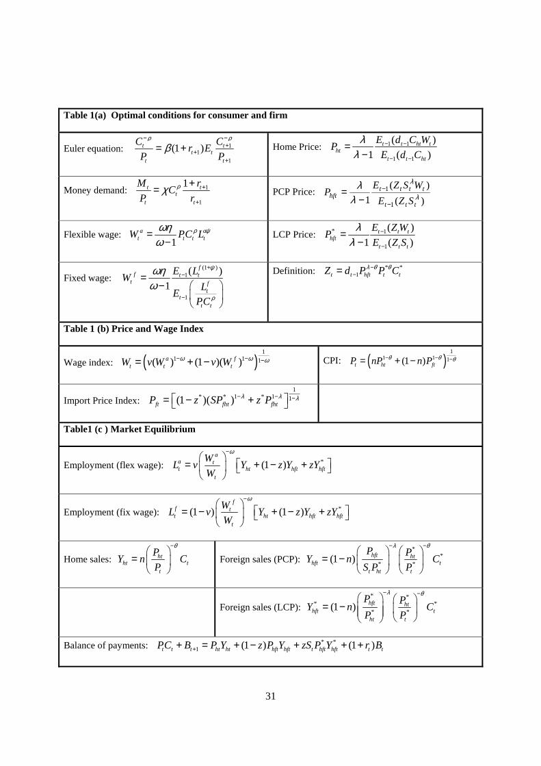
Table 1 outlines the main equations of the model. Table 1a describes the optimality conditions

for the consumer and the firm. The consumer chooses a stock of domestic currency denominated bonds

to maximize utility, given the nominal interest rate 1tr + . Money demand depends positively on

consumption and negatively on the nominal interest rate. Each consumer-worker sets the wage as a

markup over the marginal rate of substitution between consumption and hours. A fraction v of the total n

workers set wages ex-post, after the state of the world is realized, while the fraction 1-v set wages in

11

advance. The nominal discount factor used by firms in their evaluation of expected profits is now defined

as 1 11

t tt

t t

C PdC P

ρ

ρβ − −− = . That is, firms evaluate nominal profits using the same discount factor as the home

consumer (home firms are owned by home consumers). Wage and price indices are described in Table 1b.

Table 1c describes the market clearing relationships. Employment of fixed wage and flexible-

wage workers will in general differ (although the income effects of this are diversified away). The home

country current account (per capita) is equal to total income per capita less consumption. All home

consumers receive the same income, where income comes from sales to domestic consumers, foreign

consumers, through both PCP and LCP firms.

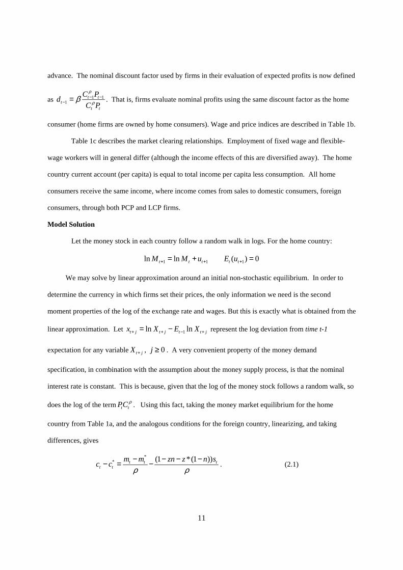
Model Solution

Let the money stock in each country follow a random walk in logs. For the home country:

1 1 1ln ln ( ) 0t t t t tM M u E u+ + += + =

We may solve by linear approximation around an initial non-stochastic equilibrium. In order to

determine the currency in which firms set their prices, the only information we need is the second

moment properties of the log of the exchange rate and wages. But this is exactly what is obtained from the

linear approximation. Let 1ln lnt j t j t t jx X E X+ + − += − represent the log deviation from time t-1

expectation for any variable t jX + , 0j ≥ . A very convenient property of the money demand

specification, in combination with the assumption about the money supply process, is that the nominal

interest rate is constant. This is because, given that the log of the money stock follows a random walk, so

does the log of the term t tPC ρ . Using this fact, taking the money market equilibrium for the home

country from Table 1a, and the analogous conditions for the foreign country, linearizing, and taking

differences, gives

** (1 *(1 ))t t t

t tm m zn z n sc c

ρ ρ− − − −− = − . (2.1)

12

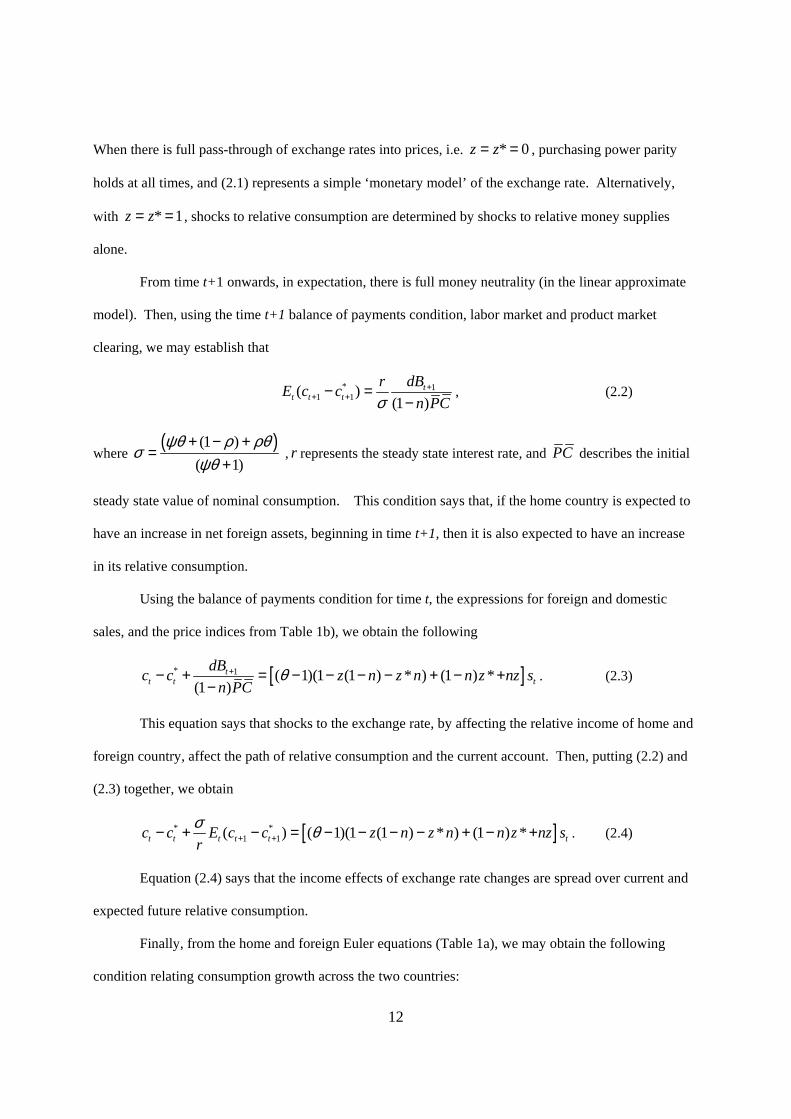
When there is full pass-through of exchange rates into prices, i.e. * 0z z= = , purchasing power parity

holds at all times, and (2.1) represents a simple ‘monetary model’ of the exchange rate. Alternatively,

with * 1z z= = , shocks to relative consumption are determined by shocks to relative money supplies

alone.

From time t+1 onwards, in expectation, there is full money neutrality (in the linear approximate

model). Then, using the time t+1 balance of payments condition, labor market and product market

clearing, we may establish that

* 11 1( )

(1 )t

t t tdBrE c c

n PCσ+

+ +− =−

, (2.2)

where ( )(1 )

( 1)ψθ ρ ρθ

σψθ

+ − +=

+ , r represents the steady state interest rate, and PC describes the initial

steady state value of nominal consumption. This condition says that, if the home country is expected to

have an increase in net foreign assets, beginning in time t+1, then it is also expected to have an increase

in its relative consumption.

Using the balance of payments condition for time t, the expressions for foreign and domestic

sales, and the price indices from Table 1b), we obtain the following

[ ]* 1 ( 1)(1 (1 ) * ) (1 ) *(1 )

tt t t

dBc c z n z n n z nz sn PC

θ+− + = − − − − + − +−

. (2.3)

This equation says that shocks to the exchange rate, by affecting the relative income of home and

foreign country, affect the path of relative consumption and the current account. Then, putting (2.2) and

(2.3) together, we obtain

[ ]* *1 1( ) ( 1)(1 (1 ) * ) (1 ) *t t t t t tc c E c c z n z n n z nz s

rσ θ+ +− + − = − − − − + − + . (2.4)

Equation (2.4) says that the income effects of exchange rate changes are spread over current and

expected future relative consumption.

Finally, from the home and foreign Euler equations (Table 1a), we may obtain the following

condition relating consumption growth across the two countries:

13

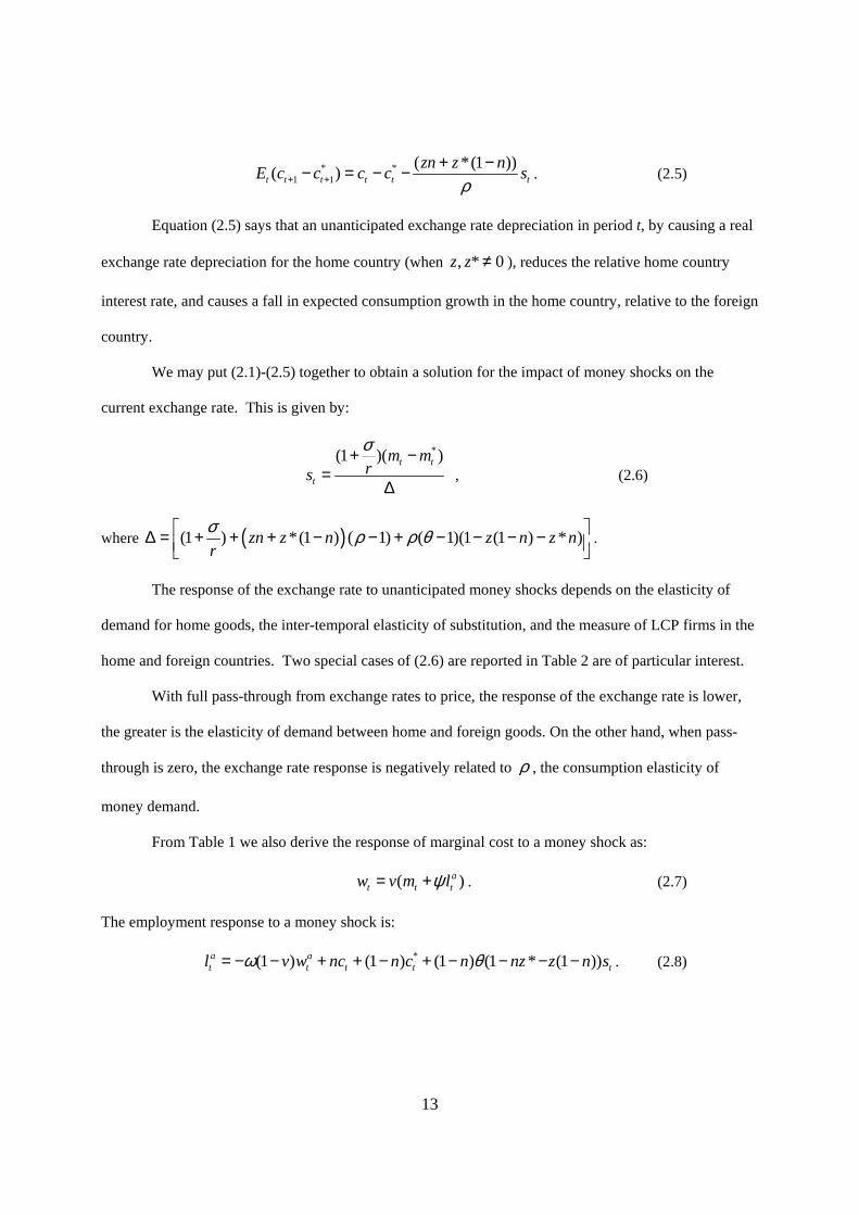
* *1 1

( *(1 ))( )t t t t t tzn z nE c c c c s

ρ+ ++ −− = − − . (2.5)

Equation (2.5) says that an unanticipated exchange rate depreciation in period t, by causing a real

exchange rate depreciation for the home country (when , * 0z z ≠ ), reduces the relative home country

interest rate, and causes a fall in expected consumption growth in the home country, relative to the foreign

country.

We may put (2.1)-(2.5) together to obtain a solution for the impact of money shocks on the

current exchange rate. This is given by:

*(1 )( )t t

t

m mrs

σ+ −=

∆ , (2.6)

where ( )(1 ) *(1 ) ( 1) ( 1)(1 (1 ) * )zn z n z n z nrσ ρ ρ θ ∆ = + + + − − + − − − −

.

The response of the exchange rate to unanticipated money shocks depends on the elasticity of

demand for home goods, the inter-temporal elasticity of substitution, and the measure of LCP firms in the

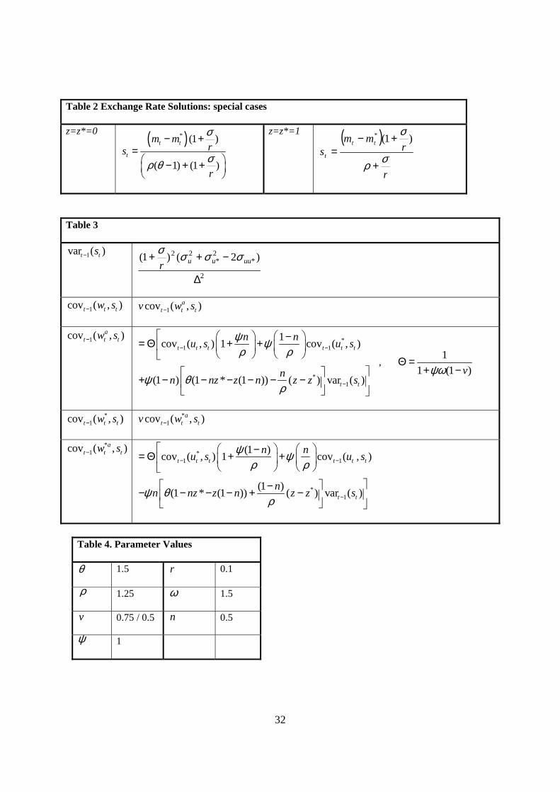
home and foreign countries. Two special cases of (2.6) are reported in Table 2 are of particular interest.

With full pass-through from exchange rates to price, the response of the exchange rate is lower,

the greater is the elasticity of demand between home and foreign goods. On the other hand, when pass-

through is zero, the exchange rate response is negatively related to ρ , the consumption elasticity of

money demand.

From Table 1 we also derive the response of marginal cost to a money shock as:

( )at t tw v m lψ= + . (2.7)

The employment response to a money shock is:

*(1 ) (1 ) (1 ) (1 * (1 ))a at t t t tl v w nc n c n nz z n sω θ= − − + + − + − − − − . (2.8)

14

Employment depends negatively upon the wage of the flexible wage setters, positively on the movement

in aggregate world consumption, and, through ‘expenditure switching’ effects, positively on the nominal

exchange rate, so long as there is some pass-through of exchange rates into prices (i.e. when , * 1z z < ).

From the money market equilibrium conditions in Table 1a, the movement in world consumption

is:

* *

* (1 ) (1 ) ( )(1 ) t t tt t

nm n m n n z z snc n cρ

+ − − − −+ − = . (2.9)

An unanticipated increase in home or foreign money raises world consumption. But in addition,

when *z z≠ , an exchange rate depreciation has a compositional impact on total consumption. For

instance, when z>z*, a depreciation raises the home CPI more than it reduces the foreign CPI. Ceteris

paribus, this implies that a weighted sum of home and foreign consumption will fall.

We now put the components of section 1 and section 2 together, examining the interaction

between the determination of exchange rates and exchange rate pass-through.

Section 3. Equilibrium Pass-through with Identical Monetary Policies

We evaluate the conditions underlying proposition 1 and its corollary, using the results from (2.6),

(2.7), and (2.8). First, define the function ),,,( 2*

2*uuzz σσΦ as the relative benefit to the firm of pricing

by LCP as opposed to PCP. That is:

2)(var

),(cov),,,( 11

2*

2* tttttuu

sswzz −− −=Φ σσ .

Because exchange rate variance and the covariance of marginal cost and the exchange rate

depend on the underlying monetary shocks, as well as on the measure of firms in each country following

LCP, we may write the function in this way. In the same way, we define ),,,( 2*

2**uuzz σσΦ as:

2)(var

),(cov),,,( 1*1

2*

2** tttttuu

sswzz −− −−=Φ σσ .

15

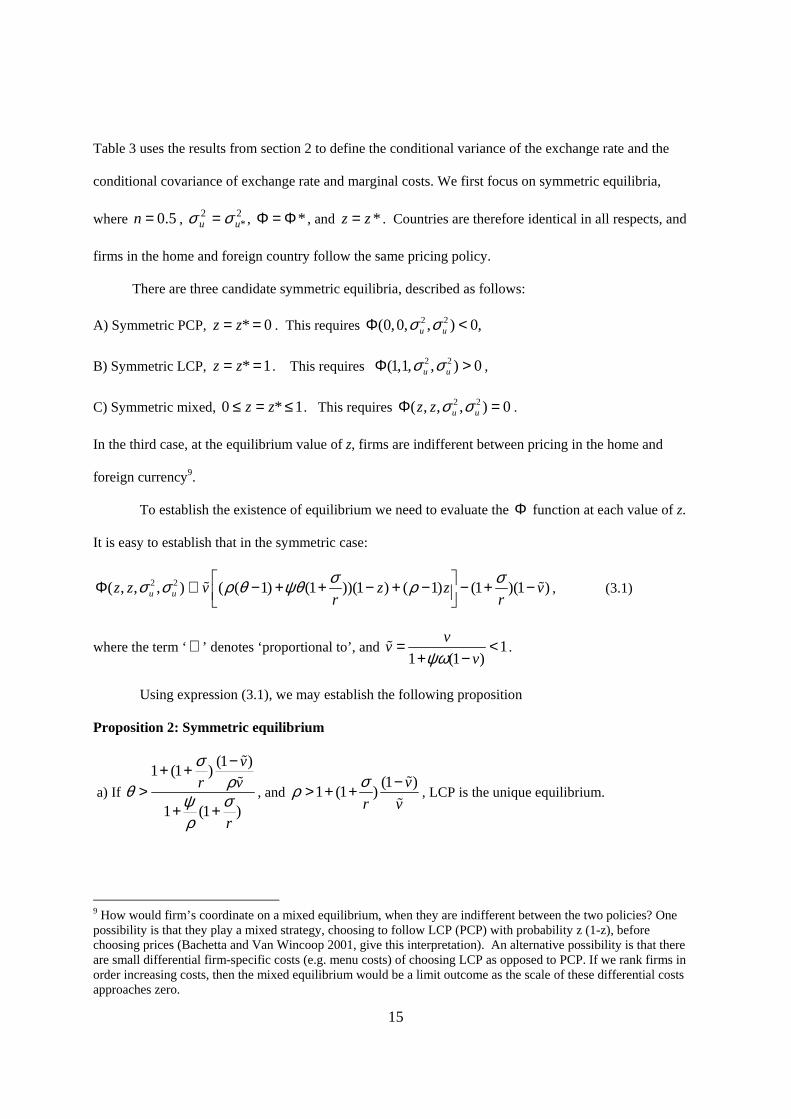
Table 3 uses the results from section 2 to define the conditional variance of the exchange rate and the

conditional covariance of exchange rate and marginal costs. We first focus on symmetric equilibria,

where 0.5n = , 2*

2uu σσ = , *Φ = Φ , and *z z= . Countries are therefore identical in all respects, and

firms in the home and foreign country follow the same pricing policy.

There are three candidate symmetric equilibria, described as follows:

A) Symmetric PCP, * 0z z= = . This requires 2 2(0,0, , ) 0,u uσ σΦ <

B) Symmetric LCP, * 1z z= = . This requires 2 2(1,1, , ) 0u uσ σΦ > ,

C) Symmetric mixed, 0 * 1z z≤ = ≤ . This requires 2 2( , , , ) 0u uz z σ σΦ = .

In the third case, at the equilibrium value of z, firms are indifferent between pricing in the home and

foreign currency9.

To establish the existence of equilibrium we need to evaluate the Φ function at each value of z.

It is easy to establish that in the symmetric case:

2 2( , , , ) ( ( 1) (1 ))(1 ) ( 1) (1 )(1 )u uz z v z z vr rσ σσ σ ρ θ ψθ ρ Φ ∝ − + + − + − − + −

% % , (3.1)

where the term ‘ ∝ ’ denotes ‘proportional to’, and 11 (1 )

vvvψω

= <+ −

% .

Using expression (3.1), we may establish the following proposition

Proposition 2: Symmetric equilibrium

a) If

(1 )1 (1 )

1 (1 )

vr v

r

σρθ ψ σ

ρ

−+ +>

+ +

%

%, and

(1 )1 (1 ) vr vσρ −> + +

%

%, LCP is the unique equilibrium.

9 How would firm’s coordinate on a mixed equilibrium, when they are indifferent between the two policies? One possibility is that they play a mixed strategy, choosing to follow LCP (PCP) with probability z (1-z), before choosing prices (Bachetta and Van Wincoop 2001, give this interpretation). An alternative possibility is that there are small differential firm-specific costs (e.g. menu costs) of choosing LCP as opposed to PCP. If we rank firms in order increasing costs, then the mixed equilibrium would be a limit outcome as the scale of these differential costs approaches zero.

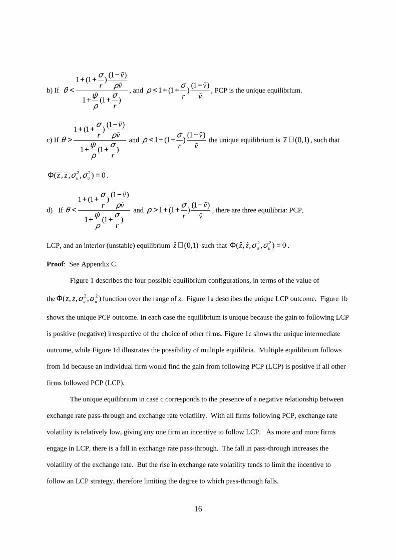
16

b) If

(1 )1 (1 )

1 (1 )

vr v

r

σρθ ψ σ

ρ

−+ +<

+ +

%

%, and

(1 )1 (1 ) vr vσρ −< + +

%

%, PCP is the unique equilibrium.

c) If

(1 )1 (1 )

1 (1 )

vr v

r

σρθ ψ σ

ρ

−+ +>

+ +

%

% and

(1 )1 (1 ) vr vσρ −< + +

%

% the unique equilibrium is (0,1)z ∈ , such that

2 2( , , , ) 0u uz z σ σΦ = .

d) If

(1 )1 (1 )

1 (1 )

vr v

r

σρθ ψ σ

ρ

−+ +<

+ +

%

% and

(1 )1 (1 ) vr vσρ −> + +

%

%, there are three equilibria: PCP,

LCP, and an interior (unstable) equilibrium ˆ (0,1)z ∈ such that 2 2ˆ ˆ( , , , ) 0u uz z σ σΦ = .

Proof: See Appendix C.

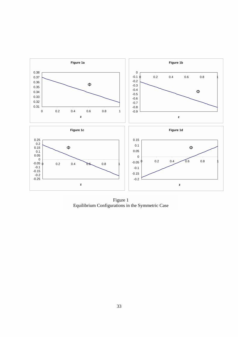
Figure 1 describes the four possible equilibrium configurations, in terms of the value of

the 2 2( , , , )u uz z σ σΦ function over the range of z. Figure 1a describes the unique LCP outcome. Figure 1b

shows the unique PCP outcome. In each case the equilibrium is unique because the gain to following LCP

is positive (negative) irrespective of the choice of other firms. Figure 1c shows the unique intermediate

outcome, while Figure 1d illustrates the possibility of multiple equilibria. Multiple equilibrium follows

from 1d because an individual firm would find the gain from following PCP (LCP) is positive if all other

firms followed PCP (LCP).

The unique equilibrium in case c corresponds to the presence of a negative relationship between

exchange rate pass-through and exchange rate volatility. With all firms following PCP, exchange rate

volatility is relatively low, giving any one firm an incentive to follow LCP. As more and more firms

engage in LCP, there is a fall in exchange rate pass-through. The fall in pass-through increases the

volatility of the exchange rate. But the rise in exchange rate volatility tends to limit the incentive to

follow an LCP strategy, therefore limiting the degree to which pass-through falls.

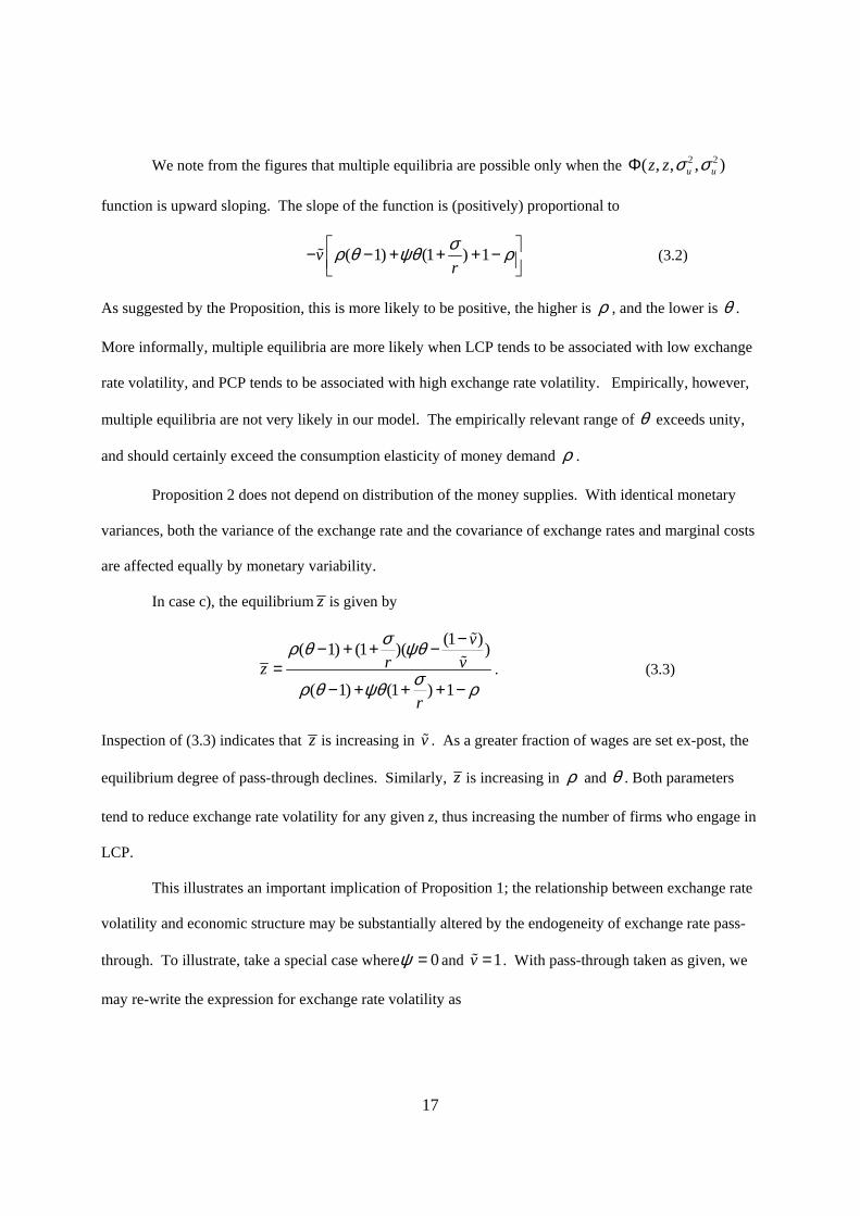
17

We note from the figures that multiple equilibria are possible only when the 2 2( , , , )u uz z σ σΦ

function is upward sloping. The slope of the function is (positively) proportional to

( 1) (1 ) 1vrσρ θ ψθ ρ − − + + + −

% (3.2)

As suggested by the Proposition, this is more likely to be positive, the higher is ρ , and the lower is θ .

More informally, multiple equilibria are more likely when LCP tends to be associated with low exchange

rate volatility, and PCP tends to be associated with high exchange rate volatility. Empirically, however,

multiple equilibria are not very likely in our model. The empirically relevant range of θ exceeds unity,

and should certainly exceed the consumption elasticity of money demand ρ .

Proposition 2 does not depend on distribution of the money supplies. With identical monetary

variances, both the variance of the exchange rate and the covariance of exchange rates and marginal costs

are affected equally by monetary variability.

In case c), the equilibrium z is given by

(1 )( 1) (1 )( )

( 1) (1 ) 1

vr vz

r

σρ θ ψθ

σρ θ ψθ ρ

−− + + −=

− + + + −

%

% . (3.3)

Inspection of (3.3) indicates that z is increasing in v% . As a greater fraction of wages are set ex-post, the

equilibrium degree of pass-through declines. Similarly, z is increasing in ρ and θ . Both parameters

tend to reduce exchange rate volatility for any given z, thus increasing the number of firms who engage in

LCP.

This illustrates an important implication of Proposition 1; the relationship between exchange rate

volatility and economic structure may be substantially altered by the endogeneity of exchange rate pass-

through. To illustrate, take a special case where 0ψ = and 1v =% . With pass-through taken as given, we

may re-write the expression for exchange rate volatility as

18

2

*2*

22

)1)(1()1(1

)2()1(

−−+−++

−++

zzr

r uuuu

θρρσ

σσσσ

.

If we begin in a situation where 1, 1θ ρ> > , so that 1z = holds (part a of the proposition), then all firms

are LCP. In this case, the exchange rate volatility is )2(1

*2*

2

2

uuuu

r

r σσσρσ

σ

−+

+

+. Here, exchange rate

volatility is less than the variance of monetary fundamentals, )2( *2*

2uuuu σσσ −+ . Now let ρ fall

below unity. Ignoring the response of pass-through, we would predict that this would increase exchange

rate volatility, so that volatility exceeded the variance of monetary fundamentals. But in our model, this

will not happen. When ρ falls below unity, part c of the proposition (or Figure 1c) applies. Now we have

pass-through falling, so that ( 1)

( 1) 1z ρ θ

ρ θ ρ−=

− + −. Exchange rate volatility is now given by

)2( *2*

2uuuu σσσ −+ . Exchange rate volatility in this example will never exceed the monetary

fundamentals.

Section 4. Pass-through with Differential Monetary Policies

We now allow for differences in money growth volatility across countries. Without loss of

generality, assume that the home country has a lower monetary growth volatility than the foreign country.

As discussed in footnote 9, we may think of equilibria where firms employ mixed strategies. Thus, if

0),,,( 2*

2* =Φ uuzz σσ and 0),,,( 2*

2** =Φ uuzz σσ we say , *z z is an equilibrium where each home

(foreign) firm chooses a probability z (z*), ex ante, of setting its export price in foreign (home) currency,

and 1-z, (1-z*) of setting its price in home (foreign) currency.

To simplify the presentation of results, we first make the additional assumption that preferences

display linearity in labor supply, so that 0ψ = . This assumption is commonly used in the literature on

19

exchange rates and price stickiness (Devereux and Engel 2001, Corsetti and Pesenti 2001). Qualitatively,

none of the results are affected by the assumption. The general case where 0ψ > is used in the

simulations below. In addition, further to our discussion of the last section, we focus only on the cases of

unique equilibrium. Thus, we restrict attention to the set of equilibria where the Φ and *Φ functions are

downward sloping.10

Using Table A1, it may be established that

2

2*

2**

2)(

)1())1(1)(1()1))(1((1~u

uu

rnznznzzn

rv

σσσσθρρσ +

+−

−−−−+−−+++∝Φ

2*

2*

2***

2)(

)1())1(1)(1()1))(1((1~u

uu

rnznznzzn

rv

σσσσθρρσ +

+−

−−−−+−−+++∝Φ

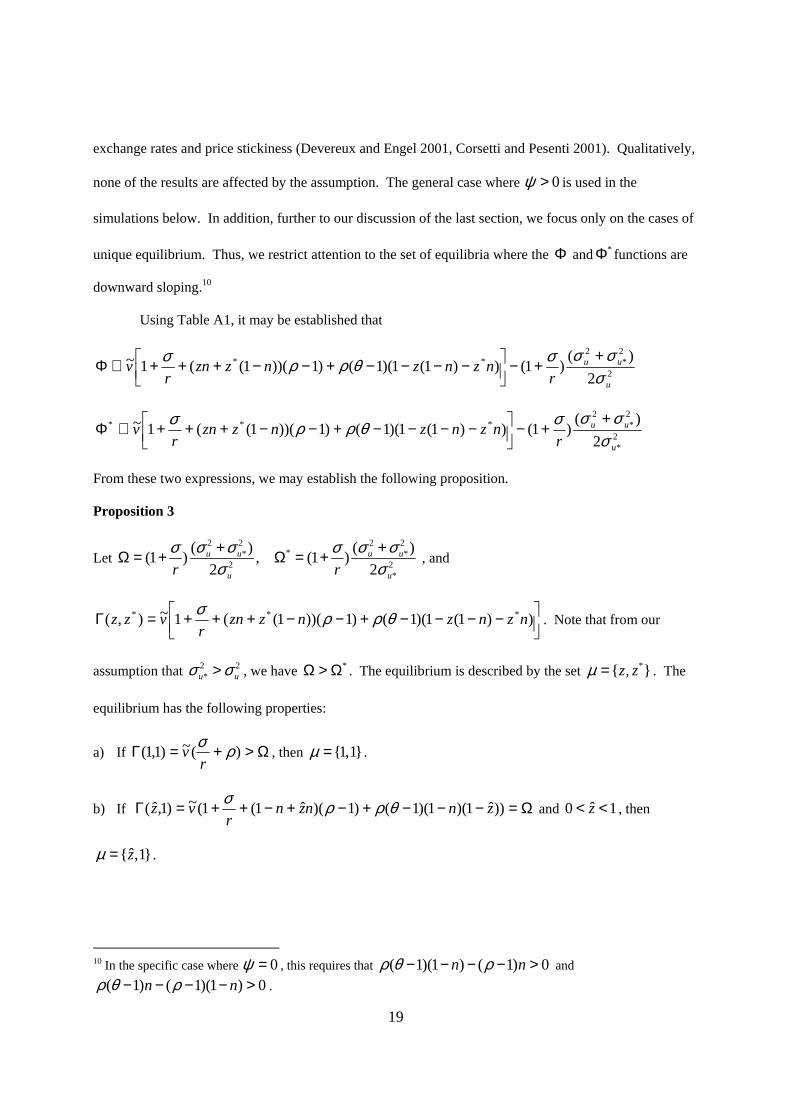
From these two expressions, we may establish the following proposition.

Proposition 3

Let 2 2 2 2

** *2 2

*

( ) ( )(1 ) , (1 )2 2

u u u u

u ur rσ σ σ σσ σ

σ σ+ +Ω = + Ω = + , and

−−−−+−−+++=Γ ))1(1)(1()1))(1((1~),( *** nznznzzn

rvzz θρρσ

. Note that from our

assumption that 2 2*u uσ σ> , we have *Ω > Ω . The equilibrium is described by the set * , z zµ = . The

equilibrium has the following properties:

a) If Ω>+=Γ )(~)1,1( ρσr

v , then 1,1µ = .

b) If Ω=−−−+−+−++=Γ ))ˆ1)(1)(1()1)(ˆ1(1(~)1,ˆ( znnznr

vz θρρσ and ˆ0 1z< < , then

ˆ ,1zµ = .

10 In the specific case where 0ψ = , this requires that ( 1)(1 ) ( 1) 0n nρ θ ρ− − − − > and

( 1) ( 1)(1 ) 0n nρ θ ρ− − − − > .

20

c) If Ω<−−+−−++=Γ<Ω ))1)(1()1)(1(1(~)1,0(* nnr

v θρρσ, then 0,1µ = .

d) If ))ˆ1)(1()1)(1(ˆ1(~)ˆ,0( **** znnzr

vz −−+−−++=Γ=Ω θρρσ and *ˆ0 1z< < , then

*ˆ0, zµ = .

e) If *))1(1(~)0,0( Ω<−++=Γ θρσr

v , then 0,0µ = .

Proof: For each part, the proof follows by direct construction. In case a), if (1,1)Γ , exceeds Ω , then full

LCP is an equilibrium for both the home and foreign firms. Moreover, because we assume that *( , )z zΓ

is decreasing in both variables (i.e. because we rule out multiple equilibria), this is the only equilibrium

outcome. In case b), a measure z of home country firms follow LCP, while all foreign firms follow

LCP. Note that z is implicitly defined by the equality ˆ( ,1)zΓ = Ω . In case c), all home country firms

follow PCP, whereas foreign firms all follow LCP. In case d), all home country firms follow PCP, while

a measure *z of foreign firms follow LCP. Finally, in case e), all firms, both home and foreign, follow

PCP.

Proposition 3 implies that the exchange rate pass-through into the home economy is always less

than or equal to that into the foreign economy. A fall in the volatility of home money growth will either

leave exchange rate pass-through into the home economy unchanged, or decrease it. Conversely,

exchange rate pass-through into the foreign country either remains unchanged, or increases. Thus, firms

tend to set their export prices in the currency that is associated with the more stable monetary growth.

Which of the five categories of Proposition 3 will come about depends on parameter values, and

the relative size of money growth variances. As in section 3, the smaller is v , the fraction of wage

contracts that are subject to ex-post adjustment, the more likely that firms in both countries will follow

PCP, since marginal costs will tend to have a smaller covariance with exchange rate movements. For a

given ρ , the greater is the elasticity of substitution between home and foreign products, θ , the more

likely is LCP, since exchange rate variance will, ceteris paribus, be smaller. When the variance of money

21

growth, relative to foreign money growth, falls to zero, exchange rate pass-through becomes complete.

The reason is that reducing money growth variance to zero tends to fully stabilize marginal cost for the

home country. With a positive exchange rate variance determined by foreign monetary instability, it is

therefore always optimal for home country firms to set prices in their domestic currency. For foreign

firms on the other hand, the variance of the exchange rate tends to fall, relative to the covariance of the

exchange rate and marginal cost, since more and more of exchange rate volatility is driven by their own

monetary shocks; the same shocks that are driving marginal costs.

Now take a particular example of the impact of changes in the variance of monetary growth and

focus on it more closely.

Proposition 4.

Begin in an initial symmetric equilibrium , z zµ = % % , where ( , ) (1 / )z z rσΓ = +% % , with 0 1z< <% . Then

a fall in the variance of home country monetary growth will reduce pass-through into the home country,

and increase pass-through into the foreign country. The new equilibrium will be either a) ',1zµ = , b)

0,1µ = , or c) *0, 'zµ = , where 'z z< % , and * 'z z> % .

Proof: Using the same arguments as Proposition 3, it is easy to show that the impact of the fall in the

variance of home country monetary growth must lead to one of cases b), c) or d) of Proposition 3. In

particular, given that the function *( , )z zΓ is common to both countries, the impact of a fall in monetary

growth in the home country is either to fully eliminate exchange rate pass-through into the domestic

economy, or to increase pass-through to 100 percent in the foreign economy. With differences in

monetary growth variance, it is no longer possible to have partial pass-through in both economies.

These results provide a theoretical rationale for the conjecture that low and stable inflation rates

may lead to a reduction in the pass-through from exchange rate movements into the CPI. In our model, a

fall in one country’s monetary instability will reduce exchange rate pass-through into that country, and

hence stabilize its price level from the effects of exchange rate movements. But the rate of pass-through

depends on relative variances of monetary growth rates, not on the absolute variances. Thus, pass-

22

through is unaffected by a parallel reduction in monetary growth stability in both countries. Moreover, a

country achieves a low degree of pass-through only by increasing exchange rate pass-through into its

trading partner.

In another sense, the model gives an additional link between inflation targeting and price stability.

In an inflation targeting country, price stability might be pursued by following a policy of low and stable

domestic-good inflation. With endogenous pass-through, there is an additional ‘bonus’ with respect to

price stability. If the country's inflation targeting policy leads to a stabilization of its money growth rate,

it encourages foreign exporters to set prices in terms of its currency. In doing so, it stabilizes the

imported goods component of its CPI, thereby further achieving price stability. But the flip side of this is

that the policy also encourages domestic exporters to favor the home currency for price setting of goods

to be sold in foreign markets. As a result the price-stability bonus achieved for the home economy comes

at the expense of a price stability ‘penalty’ imposed on the foreign economy, as its price level becomes

more unstable. In this respect, there is a type of ‘beggar-thy-neighbor’ feature in the determination of

exchange rate pass-through, and more generally in the effect of monetary policy on price stability in an

open economy with endogenous pass-through.

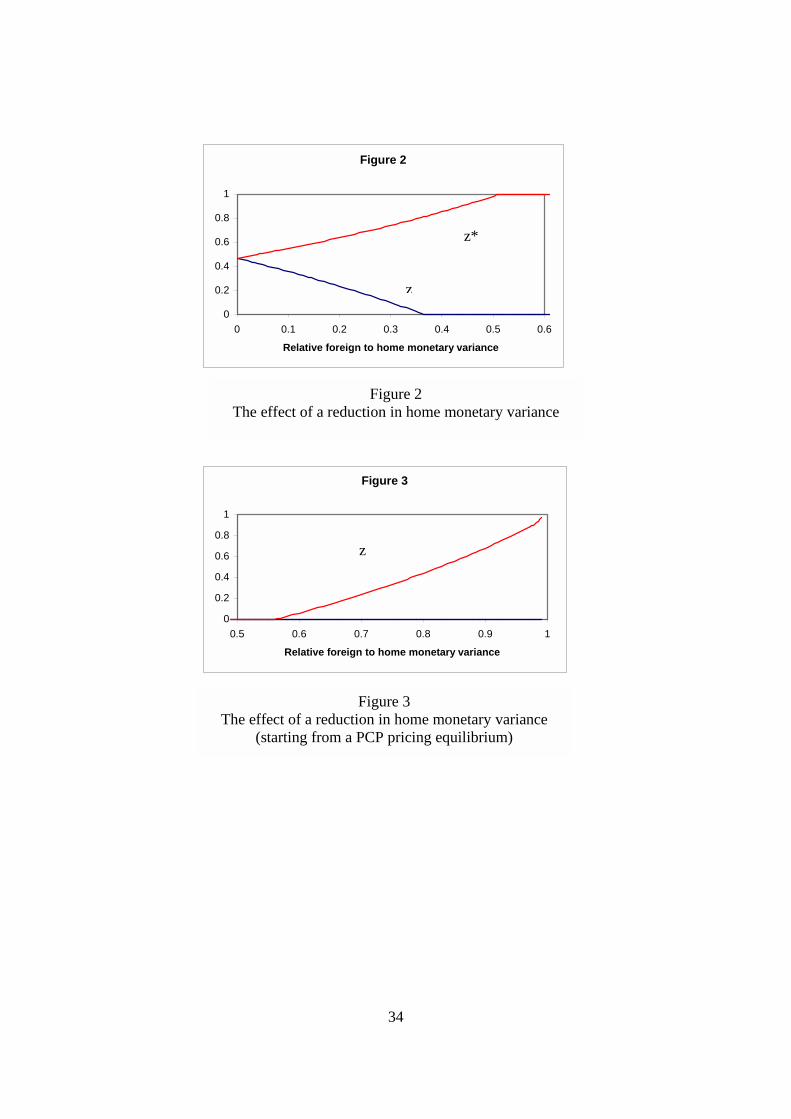
Figure 2 and 3 illustrate the results with the more general model, without the assumption of

linearity in labor supply in the utility function. Since the Φ and Φ* functions are no longer linearly

dependent (in z and z*), it is now possible that there are simultaneous interior equilibrium values for pass-

through in both countries. The parameter values used are reported in Table 4, and are mostly quite

standard.

Figure 2, shows the impact of a decline in the volatility of monetary growth in the home country,

starting from the point of equal money growth volatility. Normalizing so that the initial variances are

unity, the horizontal axis measures 2(1 )uσ− , or the percentage fall in home country monetary variance.

In this example, we assume that 75 percent of wage contracts are adjusted ex post. At the initial point,

z=z*=0.47, so there is pass-through equal to 53 percent. As 2uσ falls however, z falls sharply, and z*

23

increases, so that pass-through into the foreign economy increases to 100 percent when 2uσ falls 30

percent below 2*uσ , and pass-through into the home economy falls to zero when 2

uσ falls 50 percent

below 2*uσ .

Figure 3 illustrates the case where only 50 percent of wage contracts are adjusted ex post (v=0.5).

In this case, the initial symmetric equilibrium is one where both firms follow PCP. But as 2(1 )uσ− rises

to .55, foreign firms switch quite quickly to LCP, and z* rises to unity. Pass-through into the home

economy falls to zero. This example points quite dramatically to the importance of relative volatility of

money growth in determining exchange rate pass-through in our environment. The initial symmetric

equilibrium in this example indicates a very strong preference for PCP, given that marginal cost shows

little ex-post responsiveness to the exchange rate. But the change in relative monetary variability

increases the importance of marginal costs for foreign firms so much that they will switch over to pricing

in home currency.

Conclusions

This paper develops a general framework for analyzing the determinants of exchange rate pass-

through in an open economy macroeconomic model. We have found that the relationship between

structural parameters and exchange rate volatility can be altered dramatically when pass-through is

endogenized. This is an example of the Lucas critique – changes in economic policy may lead to changes

in equilibrium decision rules. We have given one example where changes in relative monetary stability

have very strong implications for equilibrium exchange rate pass-through in both countries. Our findings

suggest that monetary policy analysis that takes the amount of pass-through as given misses one of the

key channels through which monetary policy may work – by changing the degree of pass-through.

More generally, we conjecture that allowing for endogenous exchange rate pass-through may

have significant implications for the international transmission of shocks, for optimal monetary policy,

and for the gains from international coordination of monetary policies.

24

References

Bacchetta, Philippe, and Eric van Wincoop, 2000, “Does Exchange Rate Stability Increase Trade and Welfare?” American Economic Review 90, 1093-1109.

Bacchetta, Philippe, and Eric van Wincoop, 2001, “Trade Flows, Prices and the Exchange Rate Regime,”

in Revisiting the Case for Flexible Exchange Rates (Bank of Canada), 213-231. Bacchetta, Philippe, and Eric van Wincoop, 2002, “A Theory of the Currency Denomination of

International Trade,” Study Center Gerzensee, mimeo. Betts, Caroline and Michael B. Devereux, 1996, “The Exchange Rate in a Model of Pricing to Market,”

European Economic Review, 40, 1007-1021. Betts, Caroline and Michael B. Devereux, 2000, “Exchange Rate Dynamics in a Model of Pricing to

Market,” Journal of International Economics 50, 215-244. Chari, V.V., Patrick J. Kehoe, and Ellen R. McGrattan, 2000, “Can Sticky Price Models Generate Volatile

and Persistent Real Exchange Rates?” National Bureau of Economic Research, working paper no. 7869.

Corsetti, Giancarlo and Paolo Pesenti, 2001, “Optimal Interest Rate Rules and Exchange Rate Pass-

Through,” Federal Reserve Bank of New York, mimeo. Devereux, Michael B., 1997, “Real Exchange Rates and Macroeconomics: Evidence and Theory,”

Canadian Journal of Economics 30, 773-808. Devereux, Michael B., and Charles Engel, 2000, “Monetary Policy in the Open Economy Revisited: Price

Setting and Exchange Rate Flexibility,” National Bureau of Economic Research, working paper no. 7665.

Devereux, Michael B. and Charles Engel, 2001, “Endogenous Currency of Pricing in a Dynamic Open

Economic Model,” National Bureau of Economic Research working paper no. 8559. Devereux, Michael B., Charles Engel, and Cédric Tille, 1999, Exchange rate pass-through and the welfare

effects of the euro, National Bureau of Economic Research, working paper no. 7382. Engel, Charles, 1993, “Real Exchange Rates and Relative Prices: An Empirical Investigation,” Journal of

Monetary Economics 32, 35-50. Engel, Charles, and John H. Rogers, 1996, “How Wide is the Border?” American Economic Review 86,

1112-1125. Feenstra, Robert C., 1989, “Symmetric Pass-Through of Tariffs and Exchange Rates under Imperfect

Competition: An Empirical Test,” Journal of International Economics 27, 25-45. Feenstra, Robert C.; Joseph E. Gagnon; and, Michael M. Knetter, 1996, “Market Share and Exchange

Rate Pass-Through in World Automobile Trade,” Journal of International Economics 40, 187-207.

Friberg, Richard, 1998, “In Which Currency Should Exporters Set Their Prices?” Journal of International

Economics 45, 59-76.

25

Giovannini, Alberto, 1988, “Exchange Rates and Traded Goods Prices,” Journal of International

Economics 24, 45-68. Goldberg, Pinelopi K., 1995, “Product Differentiaton and Oligopoly in International Markets: The Case

of the U.S. Automobile Industry,” Econometrica 63, 891-951. Goldberg, Pinelopi K., and Michael M. Knetter, 1997, “Goods Prices and Exchange Rates: What Have

We Learned?” Journal of Economic Literature 35, 1243-1272. Goldberg, Pinelopi K., and Michael M. Knetter, 1998, “Measuring the Intensity of Competition in Export

Markets,” Journal of International Economics 47, 27-60. Goldberg, Pinelopi K., and Frank Verboven, 2001, “The Evolution of Price Dispersion in the European

Car Market,” Review of Economic Studies 68, 811-48. Knetter, Michael M., 1989, “Price Discrimination by U.S. and German Exporters,” American Economic

Review 79, 198-210. Knetter, Michael M., 1993, “International Comparisons of Price-to-Market Behavior,” American

Economic Review 83, 473-486. Kollmann, Robert, 2002, “Monetary Policy Rules in the Open Economy: Effects on Welfare and Business

Cycles,” Carnegie-Rochester Conference Series on Public Policy. Krugman, Paul, 1987, “Pricing to Market when the Exchange Rate Changes,” in S.W. Arndt and J.D.

Richardson, eds., Real-Finanical Linkages Among Open Economies, Cambrdige: MIT Press. Lane, Philip R., 2001, “The New Open Economy Macroeconomics: A Survey,” Journal of International

Economics. 54, 235-266. Obstfeld, Maurice, and Kenneth Rogoff, 1995, “Exchange Rate Dynamics Redux,” Journal of Political

Economy 103, 624-60. Obstfeld, Maurice, and Kenneth Rogoff, 1998, “Risk and Exchange Rates,” National Bureau of Economic

Research, working paper no. 6694. Obstfeld, Maurice, and Kenneth Rogoff, 2000, “New Directions for Stochastic Open Economy Models,”

Journal of International Economics 50, 117-153. Parsley, David C., and Shang-Jin Wei, 2001, “Explaining the Border Effect: The Role of Exchange Rate

Variability, Shipping Costs, and Geography,” Journal of International Economics 55, 87-105. Storgaard, Peter E., 2001, “Optimal Contract Currencies and Exchange Rate Policy” Chapter 4 of PhD

Thesis, University of Aarhus, and Danmarks Nationalbank, working paper 3/2002. Tille, Cédric, 2000, “‘Beggar-Thy-Neighbor’ or ‘Beggar Thyself’? The Income Effects of Exchange-Rate

Fluctuations,” Federal Reserve Bank of New York, Staff Report 112.

26

Appendix

Proof of proposition 1

From (1.4), profits under PCP are given as 1( ) ( )PCPE E S Z E S ZWλ λ λ λλ −Π = % .

This expression may be rewritten as 1( exp(ln )exp( ln )) ( exp(ln ) exp( ln )exp(ln ))E Z S E Z S Wλ λλ λ λ −% . (A1)

Now use the second order approximation:

2

exp(ln )exp( ln ) exp( ln )exp( ln )

11 var(ln ) var(ln ) cov(ln , ln )2 2

E Z S E Z E S

Z S Z S

λ λλ λ

≈ ×

+ + +

. (A2)

Using the same approximation for the expression exp(ln )exp( ln )exp(ln )E Z S Wλ , we get an approximation for profits equal to

2

12

11 var(ln ) var(ln ) cov(ln , ln )2 2

1 11 var(ln ) var(ln ) var(ln )2 2 2cov(ln , ln ) cov(ln , ln ) cov(ln , ln )

Z S Z S

Z S W

S Z Z W S W

λ

λ

λ λ

λ

λ λ

−

Σ + + +

+ + + × + + +

,

where exp( ln )exp( ln )exp((1 ) ln )E Z E S E Wλ λ λΣ = −% Taking logs, we get expected discounted profits equal to

( )

21 (1 )ln var(ln ) var(ln ) var(ln )2 2 2

cov(ln , ln ) (1 )cov(ln , ln ) (1 )cov(ln , ln )

Z S W

Z S W S Z W

λ λ

λ λ λ λ

−Σ + + + +

+ − + −. (A3)

Now, expected discounted profits under LCP are written as

[ ] [ ]1LCPE EZS EZWλ λλ −Π = % Using the same approximation, they may be written as

( )

1 (1 )ln var(ln ) var(ln ) var(ln )2 2 2

cov(ln , ln ) (1 )cov(ln , ln )

Z S W

Z S Z W

λ λ

λ λ

− Σ + + + +

+ − . (A4)

Now comparing (A3), and (A4), we can immediately establish Proposition 1.

27

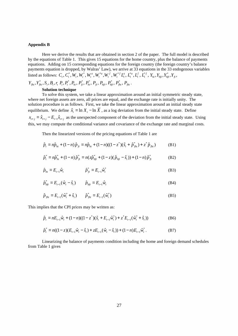
Appendix B

Here we derive the results that are obtained in section 2 of the paper. The full model is described by the equations of Table 1. This gives 15 equations for the home country, plus the balance of payments equations. Adding on 15 corresponding equations for the foreign country (the foreign country’s balance payments equation is dropped, by Walras’ Law), we arrive at 33 equations in the 33 endogenous variables listed as follows: * * * * * *, , , , , , , , , , ,a a f f a a f f

t t t t t t t t t t t tC C W W W W W W L L L L *, , , ,ht hft hft ftY Y Y Y *, , , ,fht fht t t tY Y S B r * * * * *, , , , , , , , ,t t ht ft ht ft hft hft fht fhtP P P P P P P P P P .

Solution technique To solve this system, we take a linear approximation around an initial symmetric steady state,

where net foreign assets are zero, all prices are equal, and the exchange rate is initially unity. The solution procedure is as follows. First, we take the linear approximation around an initial steady state equilibrium. We define ˆ ln lnt tx X X= − , as a log deviation from the initial steady state. Define

1ˆ ˆt j t j t t jx x E x+ + − += − as the unexpected component of the deviation from the initial steady state. Using this, we may compute the conditional variance and covariance of the exchange rate and marginal costs.

Then the linearized versions of the pricing equations of Table 1 are

* * *ˆ ˆ ˆ ˆ ˆ ˆ ˆ(1 ) (1 )((1 )( ) )t ht ft ht t fht fhtp np n p np n z s p z p= + − = + − − + + (B1) * * * * *ˆ ˆ ˆ ˆ ˆ ˆ ˆ(1 ) ( (1 )( )) (1 )t ht ft hft hft t ftp np n p n zp z p s n p= + − = + − − + − (B2) 1ˆ ˆht t tp E w−= * *

1ˆ ˆft t tp E w−= (B3) *

1ˆ ˆ ˆ( )hft t t tp E w s−= − 1ˆ ˆhft t tp E w−= (B4) *

1ˆ ˆ ˆ( )fht t t tp E w s−= + * *1ˆ ˆ( )fht t tp E w−= (B5)

This implies that the CPI prices may be written as: * * * *

1 1 1ˆ ˆ ˆ ˆ ˆ ˆ(1 )((1 )( ) ( ))t t t t t t t t tp nE w n z s E w z E w s− − −= + − − + + + (B6) * *

1 1 1ˆ ˆ ˆ ˆ ˆ ˆ((1 )( ) ( )) (1 )t t t t t t t t tp n z E w s zE w s n E w− − −= − − + − + − . (B7)

Linearizing the balance of payments condition including the home and foreign demand schedules from Table 1 gives

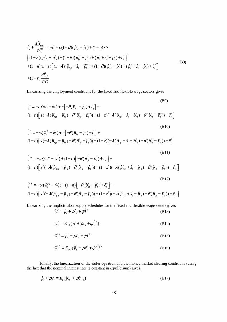
28

1

* * * * * *

* * * * *

ˆˆ ˆ ˆ ˆ(1 )( ) (1 )

ˆ ˆ ˆ ˆ ˆ ˆ ˆ ˆ(1 )( ) (1 )( ) ( )

ˆ ˆ ˆ ˆ ˆ ˆ ˆ ˆ ˆ(1 )(1 ) (1 )( ) (1 )( ) ( )

ˆ(1 )

ftt t ht t

hft ht ht t t t t t

hft t ht ht t t t t t

ft

dBc nc n p p n z

PCp p p p p s p c

n z p s p p p p s p c

dBr

PC

θ

λ θ

λ θ

++ = + − − + − ×

− − + − − + + − + + − − − − − + − − + + − +

+ +

(B8)

Linearizing the employment conditions for the fixed and flexible wage sectors gives

(B9) [ ]

* * * * * * * *

ˆ ˆ ˆ ˆ ˆ ˆ( ) ( )

ˆ ˆ ˆ ˆ ˆ ˆ ˆ ˆ ˆ ˆ(1 ) ( ( ) ( )) (1 )( ( ) ( ))

a at t t ht t t

hft ht ht t hft t ht ht t t

l w w n p p c

n z p p p p z p s p p p c

ω θ

λ θ λ θ

= − − + − − + +

− − − − − + − − − − − − +

(B10)

[ ]* * * * * * * *

ˆ ˆ ˆ ˆ ˆ ˆ( ) ( )

ˆ ˆ ˆ ˆ ˆ ˆ ˆ ˆ ˆ ˆ(1 ) ( ( ) ( )) (1 )( ( ) ( ))

f ft t t ht t t

hft ht ht t hft t ht ht t t

l w w n p p c

n z p p p p z p s p p p c

ω θ

λ θ λ θ

= − − + − − + +

− − − − − + − − − − − − +

(B11)

* * * * * *

* * *

ˆ ˆ ˆ ˆ ˆ ˆ( ) (1 ) ( )

ˆ ˆ ˆ ˆ ˆ ˆ ˆ ˆ ˆ ˆ(1 ) ( ( ) ( )) (1 )( ( ) ( ))

a at t t ft t t

fht ft ft t fht t ft ft t t

l w w n p p c

n z p p p p z p s p p p c

ω θ

λ θ λ θ

= − − + − − − + + − − − − − + − − + − − − +

(B12)

* * * * * *

* * *

ˆ ˆ ˆ ˆ ˆ ˆ( ) (1 ) ( )

ˆ ˆ ˆ ˆ ˆ ˆ ˆ ˆ ˆ ˆ(1 ) ( ( ) ( )) (1 )( ( ) ( ))

f ft t t ft t t

fht ft ft t fht t ft ft t t

l w w n p p c

n z p p p p z p s p p p c

ω θ

λ θ λ θ

= − − + − − − + + − − − − − + − − + − − − +

Linearizing the implicit labor supply schedules for the fixed and flexible wage setters gives

ˆˆ ˆ ˆa at t t tw p c lρ ψ= + + (B13)

1ˆˆ ˆ ˆ( )f f

t t t t tw E p c lρ ψ−= + + (B14) * * * *ˆˆ ˆ ˆa a

t t t tw p c lρ ψ= + + (B15) * * * *

1ˆˆ ˆ ˆ( )f f

t t t t tw E p c lρ ψ−= + + (B16)

Finally, the linearization of the Euler equation and the money market clearing conditions (using the fact that the nominal interest rate is constant in equilibrium) gives: 1 1ˆ ˆ ˆ ˆ( )t t t t tp c E p cρ ρ+ ++ = + (B17)

29

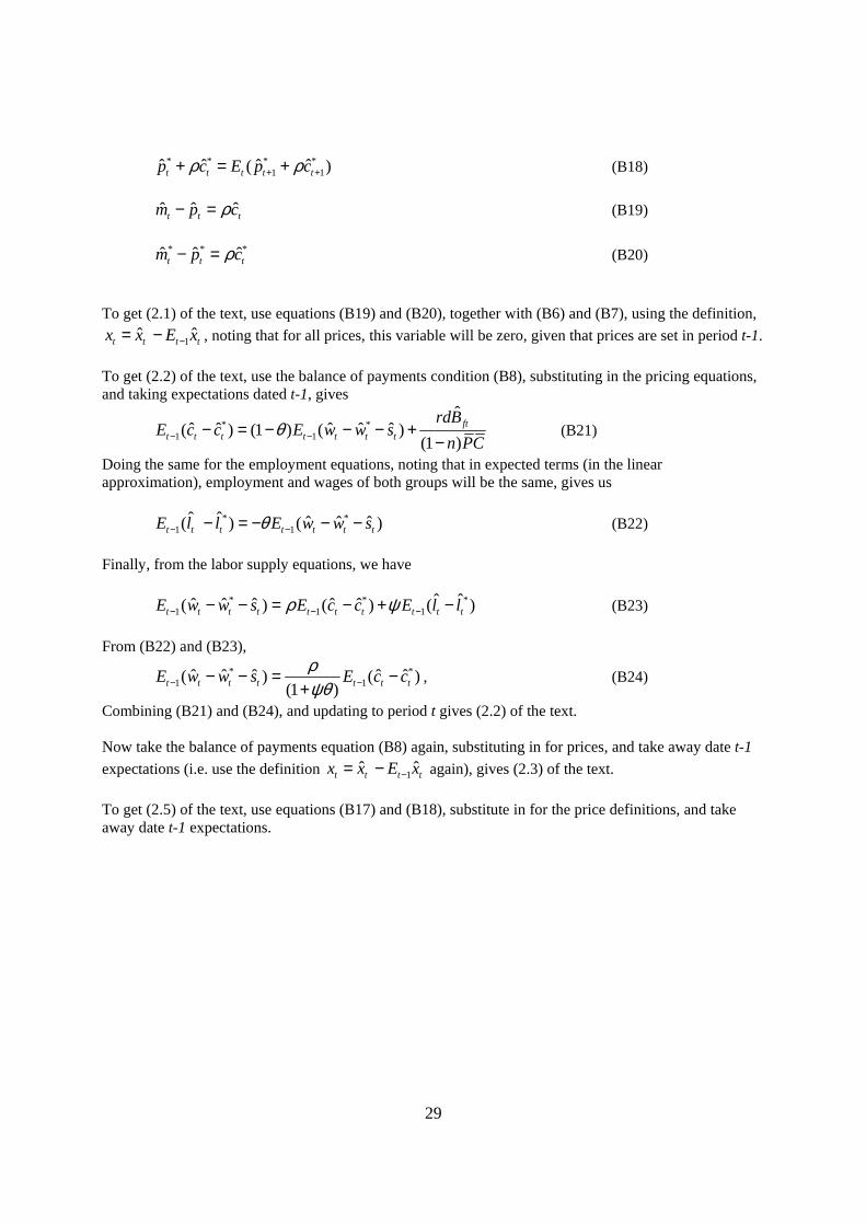
* * * *1 1ˆ ˆ ˆ ˆ( )t t t t tp c E p cρ ρ+ ++ = + (B18)

ˆ ˆ ˆt t tm p cρ− = (B19)

* * *ˆ ˆ ˆt t tm p cρ− = (B20) To get (2.1) of the text, use equations (B19) and (B20), together with (B6) and (B7), using the definition,

1ˆ ˆt t t tx x E x−= − , noting that for all prices, this variable will be zero, given that prices are set in period t-1. To get (2.2) of the text, use the balance of payments condition (B8), substituting in the pricing equations, and taking expectations dated t-1, gives

* *1 1

ˆˆ ˆ ˆ ˆ ˆ( ) (1 ) ( )

(1 )ft

t t t t t t t

rdBE c c E w w s

n PCθ− −− = − − − +

− (B21)

Doing the same for the employment equations, noting that in expected terms (in the linear approximation), employment and wages of both groups will be the same, gives us * *

1 1ˆ ˆ ˆ ˆ ˆ( ) ( )t t t t t t tE l l E w w sθ− −− = − − − (B22)

Finally, from the labor supply equations, we have * * *

1 1 1ˆ ˆˆ ˆ ˆ ˆ ˆ( ) ( ) ( )t t t t t t t t t tE w w s E c c E l lρ ψ− − −− − = − + − (B23)

From (B22) and (B23),

* *1 1ˆ ˆ ˆ ˆ ˆ( ) ( )

(1 )t t t t t t tE w w s E c cρψθ− −− − = −

+, (B24)

Combining (B21) and (B24), and updating to period t gives (2.2) of the text. Now take the balance of payments equation (B8) again, substituting in for prices, and take away date t-1 expectations (i.e. use the definition 1ˆ ˆt t t tx x E x−= − again), gives (2.3) of the text. To get (2.5) of the text, use equations (B17) and (B18), substitute in for the price definitions, and take away date t-1 expectations.

30

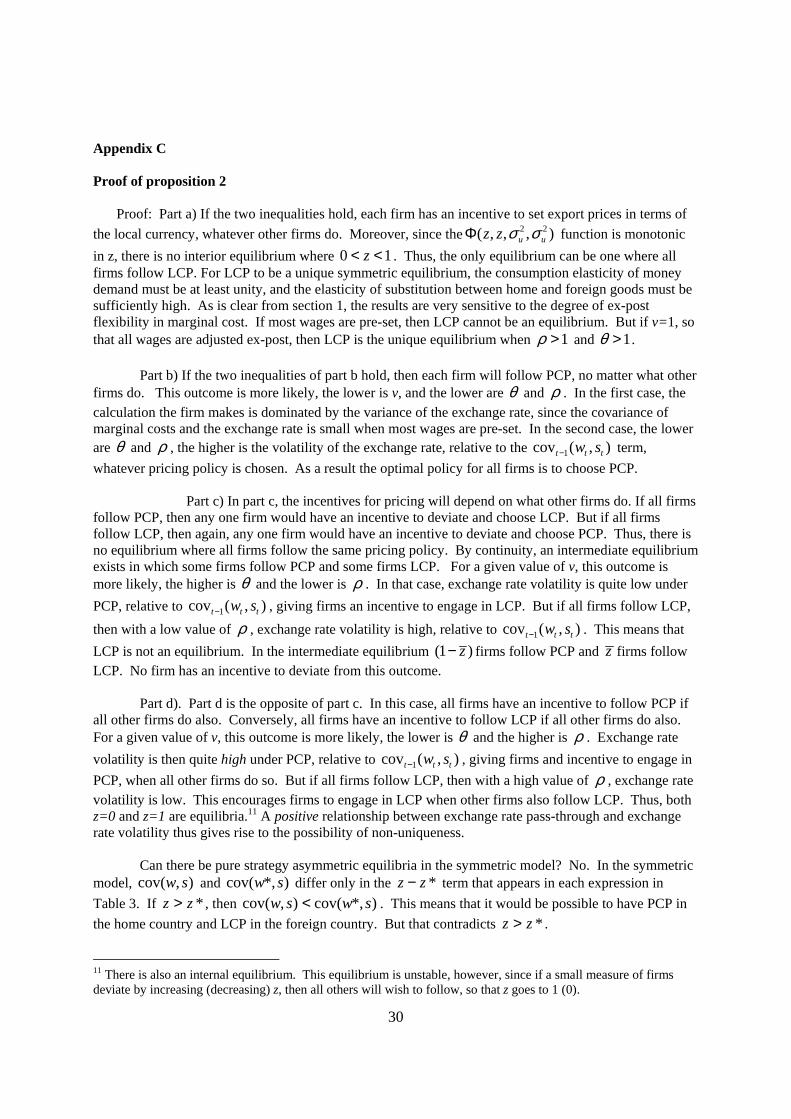
Appendix C

Proof of proposition 2

Proof: Part a) If the two inequalities hold, each firm has an incentive to set export prices in terms of the local currency, whatever other firms do. Moreover, since the 2 2( , , , )u uz z σ σΦ function is monotonic in z, there is no interior equilibrium where 0 1z< < . Thus, the only equilibrium can be one where all firms follow LCP. For LCP to be a unique symmetric equilibrium, the consumption elasticity of money demand must be at least unity, and the elasticity of substitution between home and foreign goods must be sufficiently high. As is clear from section 1, the results are very sensitive to the degree of ex-post flexibility in marginal cost. If most wages are pre-set, then LCP cannot be an equilibrium. But if v=1, so that all wages are adjusted ex-post, then LCP is the unique equilibrium when 1ρ > and 1θ > .

Part b) If the two inequalities of part b hold, then each firm will follow PCP, no matter what other firms do. This outcome is more likely, the lower is v, and the lower are θ and ρ . In the first case, the calculation the firm makes is dominated by the variance of the exchange rate, since the covariance of marginal costs and the exchange rate is small when most wages are pre-set. In the second case, the lower are θ and ρ , the higher is the volatility of the exchange rate, relative to the 1cov ( , )t t tw s− term, whatever pricing policy is chosen. As a result the optimal policy for all firms is to choose PCP.

Part c) In part c, the incentives for pricing will depend on what other firms do. If all firms follow PCP, then any one firm would have an incentive to deviate and choose LCP. But if all firms follow LCP, then again, any one firm would have an incentive to deviate and choose PCP. Thus, there is no equilibrium where all firms follow the same pricing policy. By continuity, an intermediate equilibrium exists in which some firms follow PCP and some firms LCP. For a given value of v, this outcome is more likely, the higher is θ and the lower is ρ . In that case, exchange rate volatility is quite low under PCP, relative to 1cov ( , )t t tw s− , giving firms an incentive to engage in LCP. But if all firms follow LCP,

then with a low value of ρ , exchange rate volatility is high, relative to 1cov ( , )t t tw s− . This means that LCP is not an equilibrium. In the intermediate equilibrium (1 )z− firms follow PCP and z firms follow LCP. No firm has an incentive to deviate from this outcome.

Part d). Part d is the opposite of part c. In this case, all firms have an incentive to follow PCP if all other firms do also. Conversely, all firms have an incentive to follow LCP if all other firms do also. For a given value of v, this outcome is more likely, the lower is θ and the higher is ρ . Exchange rate volatility is then quite high under PCP, relative to 1cov ( , )t t tw s− , giving firms and incentive to engage in PCP, when all other firms do so. But if all firms follow LCP, then with a high value of ρ , exchange rate volatility is low. This encourages firms to engage in LCP when other firms also follow LCP. Thus, both z=0 and z=1 are equilibria.11 A positive relationship between exchange rate pass-through and exchange rate volatility thus gives rise to the possibility of non-uniqueness. Can there be pure strategy asymmetric equilibria in the symmetric model? No. In the symmetric model, ),cov( sw and )*,cov( sw differ only in the *zz − term that appears in each expression in Table 3. If *zz > , then )*,cov(),cov( swsw < . This means that it would be possible to have PCP in the home country and LCP in the foreign country. But that contradicts *zz > .

11 There is also an internal equilibrium. This equilibrium is unstable, however, since if a small measure of firms deviate by increasing (decreasing) z, then all others will wish to follow, so that z goes to 1 (0).

31

Table 1(a) Optimal conditions for consumer and firm

Euler equation: 11

1

(1 )t tt t

t t

C Cr EP P

ρ ρ

β− −

++

+

= + Home Price: 1 1

1 1

( )1 ( )

t t ht tht

t t ht

E d C WPE d C

λλ

− −

− −

=−

Money demand: 1

1

1t tt

t t

M rCP r

ρχ +

+

+= PCP Price: )(

)(1 1

1λ

λ

λλ

ttt

tttthft SZE

WSZEP−

−

−=

Flexible wage: 1

a at t t tW PC Lρ ψωη

ω=

− LCP Price: * 1

1

( )1 ( )

t t thft

t t t

E Z WPE Z S

λλ

−

−

=−

Fixed wage: (1 )

1

1

( )1

ff t t

t ft

tt t

E LWLE

PC

ψ

ρ

ωηω

+−

−

=−

Definition: * *

1t t hft t tZ d P P Cλ θ θ−−=

Table 1 (b) Price and Wage Index

Wage index: ( )1

1 1 1( ) (1 )( )a ft t tW v W v Wω ω ω− − −= + − CPI: ( )

11 1 1(1 )t ht ftP nP n Pθ θ θ− − −= + −

Import Price Index: 1

* * 1 * 1 1(1 )( )ft fht fhtP z SP z Pλ λ λ− − − = − +

Table1 (c ) Market Equilibrium

Employment (flex wage): *(1 )a

a tt ht hft hft

t

WL v Y z Y zYW

ω−

= + − +

Employment (fix wage): *(1 ) (1 )f

f tt ht hft hft

t

WL v Y z Y zYW

ω−

= − + − +

Home sales: htht t

t

PY n CP

θ−

=

Foreign sales (PCP): *

** *(1 ) hft ht

hft tt ht t

P PY n CS P P

λ θ− −

= −

Foreign sales (LCP):

* ** *

* *(1 ) hft hthft t

ht t

P PY n CP P

λ θ− − = −

Balance of payments: * *1 (1 ) (1 )t t t ht ht hft hft t hft hft t tPC B P Y z P Y zS P Y r B++ = + − + + +

32

Table 2 Exchange Rate Solutions: special cases

z=z*=0 ( )* (1 )

( 1) (1 )

t t

t

m mrs

r

σ

σρ θ

− += − + +

z=z*=1 ( )

r

rmm

stt

t σρ

σ

+

+−=

)1(*

Table 3

1var ( )t ts−

2

*2*

22 )2()1(

∆

−++ uuuurσσσσ

1cov ( , )t t tw s− 1cov ( , )at t tv w s−

1cov ( , )at t tw s− *

1 1

*1

1cov ( , ) 1 cov ( , )

(1 ) (1 * (1 )) ( ) var ( )

t t t t t t

t t

n nu s u s

nn nz z n z z s

ψ ψρ ρ

ψ θρ

− −

−

−= Θ + +

+ − − − − − −

, 1

1 (1 )vψωΘ =

+ −

*1cov ( , )t t tw s− *

1cov ( , )at t tv w s−

*1cov ( , )a

t t tw s−

*

1 1

*1

(1 )cov ( , ) 1 cov ( , )

(1 )(1 * (1 )) ( ) var ( )

t t t t t t

t t

n nu s u s

nn nz z n z z s

ψ ψρ ρ

ψ θρ

− −

−

−= Θ + +

−− − − − + −

Table 4. Parameter Values

θ 1.5 r 0.1

ρ 1.25 ω 1.5

v 0.75 / 0.5 n 0.5

ψ 1

33

Figure 1a

0.310.320.330.340.350.360.370.38

0 0.2 0.4 0.6 0.8 1

z

Figure 1b

-0.9-0.8-0.7-0.6-0.5-0.4-0.3-0.2-0.1

00 0.2 0.4 0.6 0.8 1

z

Figure 1c

-0.25-0.2

-0.15-0.1

-0.050

0.050.1

0.150.2

0.25

0 0.2 0.4 0.6 0.8 1

z

Figure 1d

-0.2

-0.15

-0.1

-0.05

0

0.05

0.1

0.15

0 0.2 0.4 0.6 0.8 1

z

Figure 1 Equilibrium Configurations in the Symmetric Case

ΦΦ

Φ Φ

34

Figure 2

0

0.2

0.4

0.6

0.8

1

0 0.1 0.2 0.3 0.4 0.5 0.6

Relative foreign to home monetary variance

z*

z

Figure 3

0

0.2

0.4

0.6

0.8

1

0.5 0.6 0.7 0.8 0.9 1

Relative foreign to home monetary variance

z

Figure 2 The effect of a reduction in home monetary variance

Figure 3 The effect of a reduction in home monetary variance

(starting from a PCP pricing equilibrium)