Draft version November 12, 2011Preprint typeset using LATEX style emulateapj v. 08/13/06

A STABLE, ACCURATE METHODOLOGY FOR HIGH MACH NUMBER, STRONG MAGNETIC FIELD MHDTURBULENCE WITH ADAPTIVE MESH REFINEMENT: RESOLUTION AND REFINEMENT STUDIES

Pak Shing LiAstronomy Department, University of California, Berkeley, CA 94720

Daniel F. MartinLawrence Berkeley National Laboratory, 1 Cyclotron Road, Berkeley, CA 94720

Richard I. KleinAstronomy Department, University of California, Berkeley, CA 94720;

and Lawrence Livermore National Laboratory, P.O.Box 808, L-23, Livermore, CA 94550

and

Christopher F. McKeePhysics Department and Astronomy Department, University of California, Berkeley,

CA 94720

Draft version November 12, 2011

ABSTRACT

Performing a stable, long duration simulation of driven MHD turbulence with a high thermal Machnumber and a strong initial magnetic field is a challenge to high-order Godunov ideal MHD schemesbecause of the difficulty in guaranteeing positivity of the density and pressure. We have implemented arobust combination of reconstruction schemes, Riemann solvers, limiters, and Constrained TransportEMF averaging schemes that can meet this challenge, and using this strategy, we have developed a newAdaptive Mesh Refinement (AMR) MHD module of the ORION2 code. We investigate the effects ofAMR on several statistical properties of a turbulent ideal MHD system with a thermal Mach numberof 10 and a plasma β0 of 0.1 as initial conditions; our code is shown to be stable for simulations withhigher Mach numbers (Mrms = 17.3) and smaller plasma beta (β0 = 0.0067) as well. Our results showthat the quality of the turbulence simulation is generally related to the volume-averaged refinement.Our AMR simulations show that the turbulent dissipation coefficient for supersonic MHD turbulenceis about 0.5, in agreement with unigrid simulations.

Subject headings: Magnetic fields—MHD—ISM: magnetic fields—ISM: kinematics and dynamics—stars:formation—methods: numerical—turbulence

1. INTRODUCTION

Eulerian codes are commonly used in star formationstudies in order to model the complex physical processesinvolved, including turbulence, magnetic fields, gravita-tional collapse, and radiation feedback. The dynamicranges of density and size scales involved in star forma-tion are enormous, ranging from more than 10 pc in giantmolecular clouds (GMCs) of density ∼ 5 AU protostellarcores with densities & 1013 cm−3 (Masunaga et al. 1998).This poses a significant challenge to numerical simula-tions using a uniform computational mesh. For example,using the unigrid code ZEUS-MP (Hayes et al. 2006), asimulation of ideal MHD turbulence with a 10243 grid re-quires ∼ 50, 000 cpu hours. When gravitational collapsebegins, dense cores will reach the numerical resolutionlimit (Truelove et al. 1997) in just a small fraction ofthe global free-fall time, tff . For a high-order Godunovscheme, the computing time will be ∼ 5 times that forZEUS-MP, which uses a low-order scheme. The comput-ing time is further increased by a factor of at least 16whenever the resolution of the 3D grid is doubled be-

Electronic address: psli@astron.berkeley.eduElectronic address: DFMartin@lbl.govElectronic address: klein@astron.berkeley.eduElectronic address: cmckee@astro.berkeley.edu

cause maximum Alfven speed will be increased at lowerdensity regions as the result of higher resolution. It iscomputationally inefficient to simply increase the gridresolution for star formation simulations because only asmall fraction of the simulated region has collapsed tosufficiently high density to violate numerical resolutionrequirements; most of the simulated volume is in lowdensity voids where such fine resolution is unnecessary.Therefore, adaptive mesh refinement (AMR) becomes animportant tool for simulation of star formation using Eu-lerian codes. With AMR, the computational mesh is re-fined only in the localized regions where high resolutionis required, and as a result computational resources areconcentrated in the regions where they are needed most.

Stars form in molecular clouds, which are cold (T ∼10 K), supersonically turbulent (sonic Mach numbers∼ 10 on scales ∼ 10 pc), and magnetized (B & 10µG);the Alfven Mach number is observed to be of order unityand the plasma β parameter is small (. 0.1; Crutcher1999). There are several MHD codes with AMR ca-pability, including the publicly available codes Ramses(Teyssier 2002), PLUTO (Mignone et al. 2007), ENZO(Wang & Abel 2009), and FLASH (Fryxell et al. 2000).However, to our knowledge, there is no AMR code in theliterature that has demonstrated the capability of simu-

2 Li, McKee, & Klein

lating supersonic MHD turbulence with initial conditionsappropriate for star-forming regions. The primary rea-son for this is that Godunov schemes for ideal MHD withhigh-order approximate Riemann solvers cannot guar-antee positivity in density and pressure (e.g. LeVeque1992; Toro 1999; Berthon 2005; Zhang & Shu 2010) andare therefore unstable for turbulence that is driven forlong times with such initial conditions. This becomes animportant consideration when developing an AMR idealMHD code for star formation simulations with MHD tur-bulence.

Because turbulence is intermittent, one might hopethat AMR would be very effective in simulating it. How-ever, in a study of purely hydrodynamic turbulence usingthe ENZO code, Kritsuk et al. (2006) argued that the useof AMR only became practical from an efficiency stand-point if the base mesh had high resolution to start with.When they attempted runs with coarse (1283 and 2563)base meshes (note that they used refinement ratios of 4),a large fraction of their domain was refined until theywere sufficiently able to resolve the localized turbulentstructures using AMR: with the refinement criterion theyadopted, they refined 90% of the computational domainat 5123 resolution, 65% of the domain at 10243 resolu-tion and 34% at 20483 resolution. Furthermore, it is notjust a matter of whether AMR is economical for a turbu-lence simulation, but also whether it can accurately cap-ture the properties of the turbulence. Another attemptat using different refinement criteria, such as refining onlocal vorticity and divergence of velocity in addition toshock refinement for purely hydrodynamic turbulence,also shows that very large refinement coverage generallyresults in capturing the turbulence statistics (Schmidt etal. 2009).

In this paper, we present a robust MHD AMR schemethat is able to simulate turbulent flows with high Machnumbers and strong initial magnetic fields and that usesan accurate CT scheme to maintain ∇ · B = 0 to ma-chine accuracy without recourse to approximate methodsthat rely on either divergence cleaning(e.g. Crockett etal. 2005) or monopole advection (Powell’s 8-wave schemeand its extensions; e.g. Powell et al. 1999; Dedner et al.2002; Mignone et al. 2007; Wang & Abel 2009; Waa-gan et al. 2011). Recently, Waagan (2009) modified theMHD module of the FLASH code using a directionallysplit MUSCL-Hancock scheme with properly discretizedPowell source terms in order to enable stable driven-turbulence simulations. The driven-turbulence tests inWaagan et al. (2011) are either at high Mach numberswith a relatively weak initial magnetic field (β0 ∼ 1)or at low thermal Mach numbers (. 2) with somewhatstronger fields (β0 ∼ 0.25). The tests they carried outwere all unigrid; the performance of their code on driventurbulence with AMR was not described. Waagan etal. (2011) cites simulations of driven turbulence at highMach numbers in strong fields using this code, but thesetoo were unigrid simulations.

Here we present the results of a quantitative inves-tigation of simulations of ideal MHD turbulence usinga newly implemented ideal MHD module in our AMRcode, ORION2, which is based on a conservative high-order Godunov scheme. We investigate the significanceof refinement coverage to the quality of turbulence statis-tics in strongly supersonic MHD turbulent flow. We are

able to perform long duration, high Mach number, drivenMHD turbulence simulations with a magnetic field thatis initially moderately strong (β0 = 0.1). In §2, webriefly describe the numerical method and the implemen-tation of our AMR constrained transport scheme usingthe Chombo AMR framework (Colella et al. 2000). In§3, we present several standard tests to examine the ac-curacy of the code for both unigrid and AMR simula-tions. In §4 we discuss the effects of refinement coverageon several ideal MHD turbulence statistics using AMR.We focus our discussion on the velocity power spectrum,the PDF, and the turbulence dissipation rates. In §5 wepresent our conclusions.

2. NUMERICAL METHOD

2.1. ORION2

In this paper we present ORION2, which representsa major upgrade of our parallel radiation hydrodynamicAMR code ”ORION” (Truelove et al. 1998; Klein 1999;Krumholz et al. 2004, 2007). ORION2 is implementedusing the Chombo AMR framework (Colella et al. 2000)and is in a modular form that allows the selection ofa variety of physics modules for simulations. Chombois a set of highly optimized tools that provide an in-frastructure for implementing finite difference and finitevolume methods for solving partial differential equationson a block-structured AMR grid configuration. Ellipticand time-dependent modules are included, as well as sup-port for parallel platforms using MPI. The newly devel-oped MHD module of ORION2 is based on the Godunovscheme in the finite volume formalism implemented inthe PLUTO code (Mignone et al. 2007). Specifically,we use a dimensionally unsplit Corner Transport Up-wind (CTU) scheme (Colella 1990) incorporating theConstrained Transport (CT) framework (Evans & Haw-ley 1988). This CTU+CT integrator is best describedin Stone et al. (2008), which will not be repeated here.Our implementation preserves some of the flexibility ofthe PLUTO code in choosing (1) different interpolationschemes to re-construct cell interface states from the cell-center values, such as the piecewise linear method (PLM)or the piecewise parabolic method (PPM); (2) differ-ent limiters for the preservation of monotonicity near adiscontinuity during the re-construction stage, from thevery diffusive minmod to least diffusive monotonized cen-tral difference limiter; (3) different Riemann solvers, suchas Roe and HLL-family solvers, to obtain fluxes at thecell interfaces based on the reconstructed cell interfacestates; and (4) different CT electromotive force (EMF)averaging schemes, such as the simple arithmetic aver-aging of fluxes computed during the upwind step (Bal-sara & Spicer 1999), or a face-to-edge integration pro-cedure using the arithmetic average of the EMF deriva-tives from neighbor cells, or selecting EMF derivativesaccording to the sign of the mass flux at the cell inter-face. See Gardiner & Stone (2005) on how to computethe EMF at cell edges during the upwind step. Mignoneet al. (2007) have summarized the advantages and dis-advantages of the combinations of different solvers andintegration schemes.

The CT scheme increases the complexity of the algo-rithm, especially for an AMR code, and it requires ad-ditional memory for storing the face-centered magneticfield. However, the benefit of the CT scheme is that the

MHD Turbulence Resolution and Refinement Study with AMR 3

solenoidal constraint ∇ · B = 0 is ensured to machine ac-curacy. For cell-centered MHD algorithms, divergence-cleaning methods (e.g. Crockett et al. 2005) are used toensure the solenoidal constraint, but they cannot guaran-tee positivity of pressure (or energy) and therefore reducethe robustness of the code. The Dedner et al. (2002) ap-proach, which is used in some cell-centered codes (e.g.Peng & Abel 2009; Mignone & Tzeferacos 2010), allowsmagnetic monopoles to decay with time as they are trans-ported to the domain boundaries. Some studies havereported that monopoles could lead to incorrect jumpconditions and other spurious dynamical effects (e.g Bal-sara & Spicer 1999; Toth 2000). The cell-centered fieldis readily calculated with the CT scheme: once the face-centered magnetic field is updated, the cell-centered mag-netic field is computed from a simple averaging of theface-centered magnetic fields.

2.2. AMR Implementation

Extending any uniform-mesh algorithm to AMR re-quires several modifications, primarily involving the cou-pling between the solutions at different resolutions. Wefollow the block-structured AMR approach outlined byBerger and Colella (1989) and extended to MHD by Bal-sara (2001).

We begin with a uniform mesh that spans the domainand is denoted as AMR level ` = 0, with mesh spacingh0. (Superscripts on the symbols h, nref , t and ∆t indi-cate the level of refinement, not a power.) When refine-ment is triggered by some criterion, such as a steep den-sity, velocity or magnetic field gradient, refined grids areconstructed in logically-rectangular patches with meshspacing h1 = h0/n0

ref , which are grouped into AMR level1; here the refinement ratio n0

ref is some power of 2. Iffurther refinement is desired, more AMR levels are con-structed. Each AMR level ` has a uniform mesh spacingh` = h`−1/n`−1

ref . In general, n`ref can have a non-uniform

dependence on `, but in this paper we adopt n`−1ref = 2.

Patches with the same resolution are organized into lev-els, which are then organized into a hierarchy of AMRlevels.

Following the approach outlined by Berger and Colella(1989), we refine in time as well as space, commonlyknown as “subcycling” – the solution on each AMR levelis updated using a timestep ∆t` = ∆t`−1/n`−1

ref . If weknow the solution on the entire AMR hierarchy at timet0, then we begin the multilevel update of the solutionon all levels by updating the base level solution by ∆t0,without regard for any finer levels. We then recursivelyadvance any refined levels until the solution on the en-tire AMR hierarchy has reached t0 + ∆t0. Wheneverthe solutions on different levels reach the same solutiontime, they are “synchronized”, to ensure that the com-posite solution remains conservative and maintains thesolenoidal nature of the magnetic field.

In general, the update of the solution on each logically-rectangular patch follows the same approach as that for auniform-mesh implementation. AMR-specific implemen-tation details fall into the following categories:

1) Boundary conditions: Following common prac-tice, boundary conditions at the edge of a rectan-gular patch are handled by adding a ring of ghostcells around the patch sufficient to complete the

stencils used to update the solution on the inte-rior of the patch (otherwise known as the “validregion”). The algorithm in this work requires 4ghost cells. Solution values in ghost cells (and themagnetic fields on the associated “ghost faces”) arefilled depending on the type of boundary they areassociated with:

1.1) Physical domain boundaries – if the patchboundary abuts a (non-periodic) physical do-main boundary, ghost cell values are set usingstandard discretizations of the relevant physi-cal domain boundary condition (e.g. Dirichletor Neumann boundary conditions).

1.2) Copy boundaries – if the patch is adjacent toother patches on the same level, ghost-cell val-ues are filled by copying interior (valid-region)values from adjacent patches.

1.3) Coarse-fine boundaries – if the ghost cellsare along a coarse-fine boundary between twoAMR levels, coarse-level solution values areinterpolated to fill in ghost regions. If thefine level is not at the same solution timet as the coarse-level solution, we interpolatethe coarse-level data linearly in time, sincet`−1old ≤ t` ≤ t`−1

new. Cell-centered conservedquantities are filled using piecewise linear in-terpolation that is limited to prevent the cre-ation of new maxima and minima, followingBerger and Colella (1989). The face-centeredmagnetic field is interpolated by first per-forming a piecewise-linear interpolation of thecoarse-level field onto the fine-level faces thatoverlie the coarse-level faces, and then linearlyinterpolating these interpolated values in theface-normal direction to fill the fine-level facesthat do not overlie coarse-level faces. Notethat this differs from the divergence-free inter-polation scheme presented by Balsara (2001)in that interpolated values are not necessarilydivergence free. We have not found it nec-essary to ensure that the magnetic fields inghost regions are divergence-free, because theinterpolated ghost values are used only in thereconstruction scheme to compute the fluxesin the divergence-preserving CT scheme andare never directly used to increment the mag-netic fields themselves.

2) Interpolation to newly-refined regions: Asthe solution evolves, the refined regions evolve withit through a regridding process. Previously re-fined regions are de-refined when finer resolutionis no longer needed, while coarse-level regions arerefined when finer resolution is required. In the de-refinement case, we simply average the fine-levelsolution to the newly-exposed coarse-level mesh.Newly-refined regions are filled by interpolatingthe coarse-level solution. Cell-centered conservedquantities are interpolated using piecewise linearinterpolation that is limited to prevent the cre-ation of new solution maxima and minima. Theface-centered magnetic field is defined using a two-step process. First, we interpolate the coarse-level

4 Li, McKee, & Klein

B field onto the new faces using the face-centeredinterpolation used to fill ghost faces at coarse-fineinterfaces. Then, the newly interpolated values areprojected using a variant of the face-centered pro-jection described in Martin & Colella (2000) to en-sure that they are discretely divergence-free.

3) Synchronization: When the solutions on twoAMR levels reach the same time, a series of syn-chronization operations is performed. First, thefine-level solution is averaged onto the covered re-gions of the coarser level. This includes both cell-centered conserved variables and the face-centeredB. The coarse- and fine-level solutions have beenupdated using fluxes that have been computed in-dependently, likely resulting in a loss of conserva-tion at coarse-fine interfaces. Conservation is main-tained through a flux-correction step similar to thatused by Berger and Colella (1989), which ensuresthat the same fluxes are used to update the coarse-and fine-level solutions across coarse-fine interfaces.

Similarly, the magnetic field is unlikely to bedivergence-free at coarse-fine interfaces becausecoarse- and fine-level magnetic fields have been up-dated independently. Following Balsara (2001), weensure a divergence-free B at coarse-fine interfacesthrough a correction step that ensures that thesame electric field values are used to update thecoarse- and fine-level B field adjacent to coarse-fineinterfaces.

3. STANDARD TEST RESULTS

We have performed many tests of the ORION2 MHDmodule, including the well-known standard tests, suchas the EM wave families (e.g. Crockett et al. 2005), theRyu & Jones (1995) shock-tube tests, the Brio & Wu(1988) shock-tube test, the field-loop advection test, andthe MHD blast-wave test as in Gardiner & Stone (2005).We present the results of only two of the shock-tube testsand the field-loop advection test here to demonstrate thesecond-order accuracy of the MHD module.

3.1. Shock-tube Tests

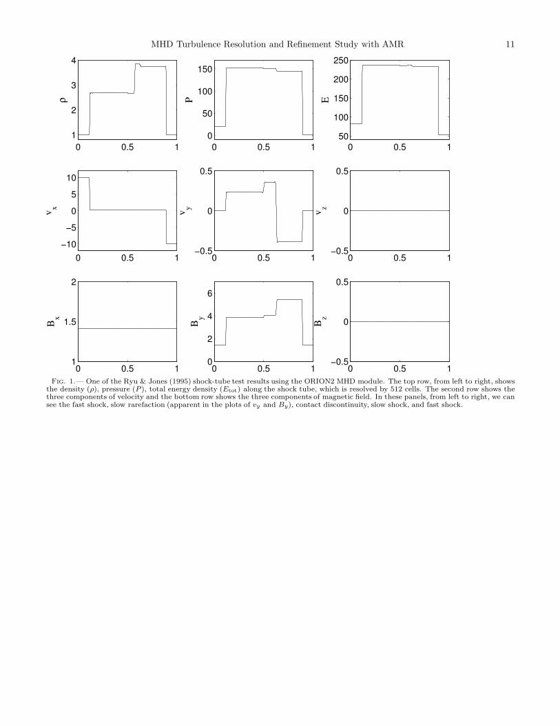
Ryu & Jones (1995) developed a suite of shock-tube tests that are commonly used for testingMHD algorithms. In Figure 1, we present theresults of just one of the tests with the set-ting of initial conditions (ρ, vx, vy, vz, Bx, By, Bz, P ) =

(1, 10, 0, 0, 5/(4π)1/2, 5/(4π)1/2, 0, 20) on the left and(1,−10, 0, 0, 5/(4π)1/2, 5/(4π)1/2, 0, 1) on the right of thecontact discontinuity; here ρ is the density, v the veloc-ity and P the gas pressure. The contact discontinuity islocated at the middle of the shock tube, and we set theadiabatic index of the gas to be γ = 5/3. The lengthof the shock tube is 1 and is resolved by 512 cells alongthe x-direction. The initial condition on the velocity is acolliding flow with a magnetic field at an angle of 45◦ inthe x− y plane. The results at a time 0.08 in code units(corresponding to 0.46 sound crossing times at the leftside of the shock tube initially) are shown in Figure 1,and they agree with the magnitudes and locations of theshocks found by Ryu & Jones (1995) to almost withinthe thickness of the lines.

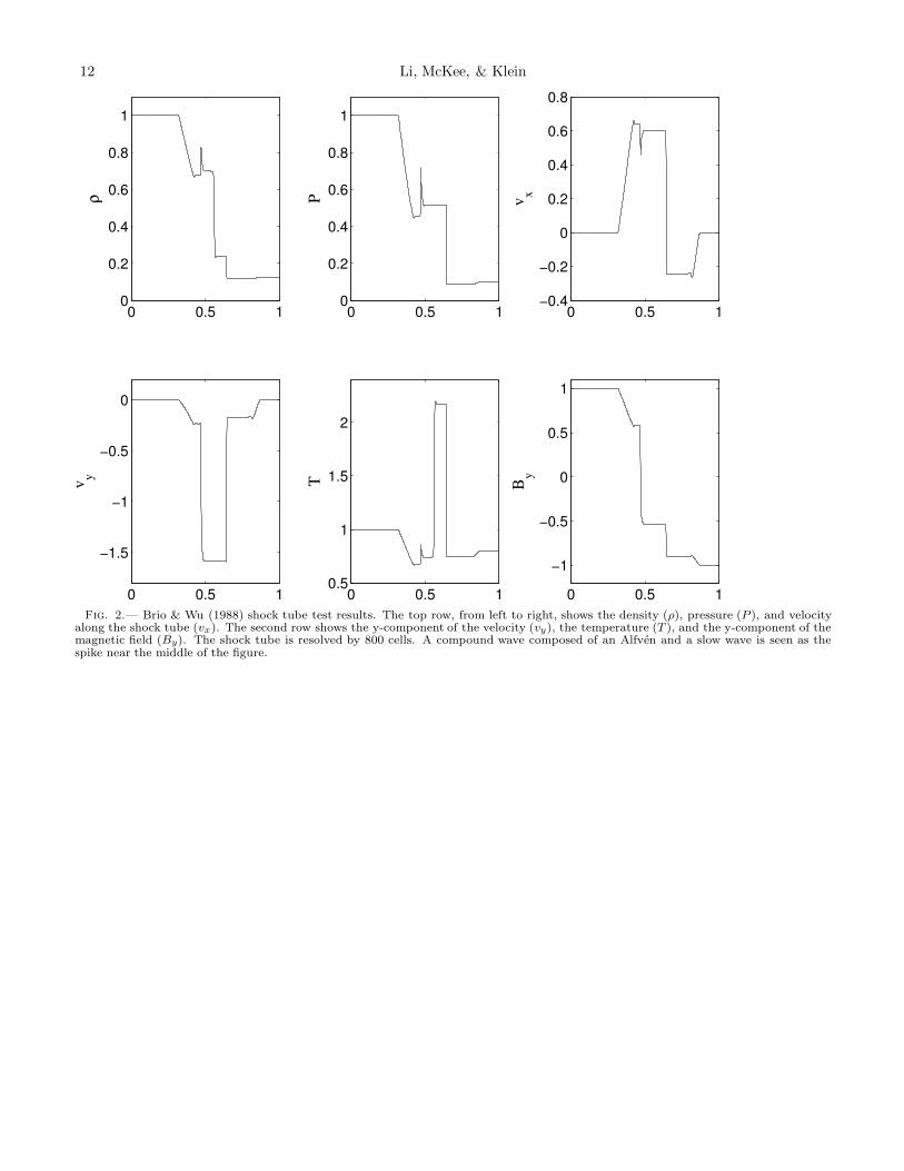
In Figure 2, we show the results of another com-monly used shock-tube problem, that of Brio & Wu(1988) . The initial conditions of this test are(ρ, vx, vy, vz, Bx, By, Bz, P ) = (1, 0, 0, 0, 0.75, 1, 0, 1) onthe left and (0.125, 0, 0, 0, 0.75,−1, 0, 0.1) on the right;here P is the gas pressure. The contact discontinuity islocated at the middle of the shock tube and γ = 2. Thelength of the shock tube is 1 and is resolved by 800 cellsalong the x-direction. The gas has no movement initially.The y-component of the magnetic field changes sign atthe contact discontinuity and has a pressure jump of 10.Figure 2 shows the results at a time of 0.1 (correspondingto 0.14 sound crossing times at the left side of the shocktube initially). We can see the compound wave, whichis composed of an Alfven wave and a slow wave, in thefigure.

3.2. Field-Loop Advection

Since Gardiner & Stone (2005) first suggested using theadvection of a magnetic field loop to show the differencebetween operator split and unsplit schemes, field-loopadvection has become a standard test for MHD algo-rithms. Our setup of the 3D test is exactly the same asin Gardiner & Stone (2008): the magnetic field loop iscreated inside a rectangular box of size (2,1,1) resolvedon a 2N×N×N grid with periodic boundaries. The loopof magnetic field is generated from a vector potential ona coordinate system (x1, x2, x3), with A1 = A2 = 0 and

A3 =

{

B0(R − r) for r ≤ R,0 for r > R, (1)

where B0 = 10−3, r =√

x21 + x2

2, and the size of theloop is R = 0.3. The computational coordinate system(x, y, z) is transformed to (x1, x2, x3) by

x1 = (−2x + z)/√

5,

x2 = y, (2)

x3 = (x + 2z)/√

5,

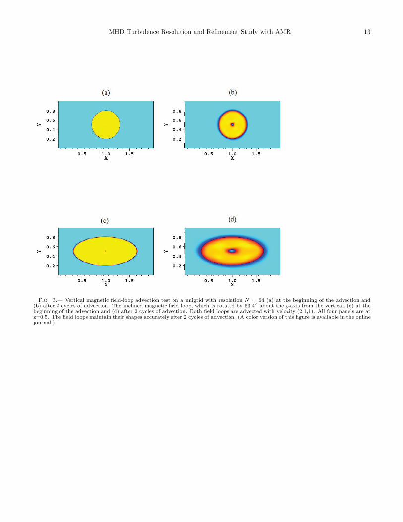
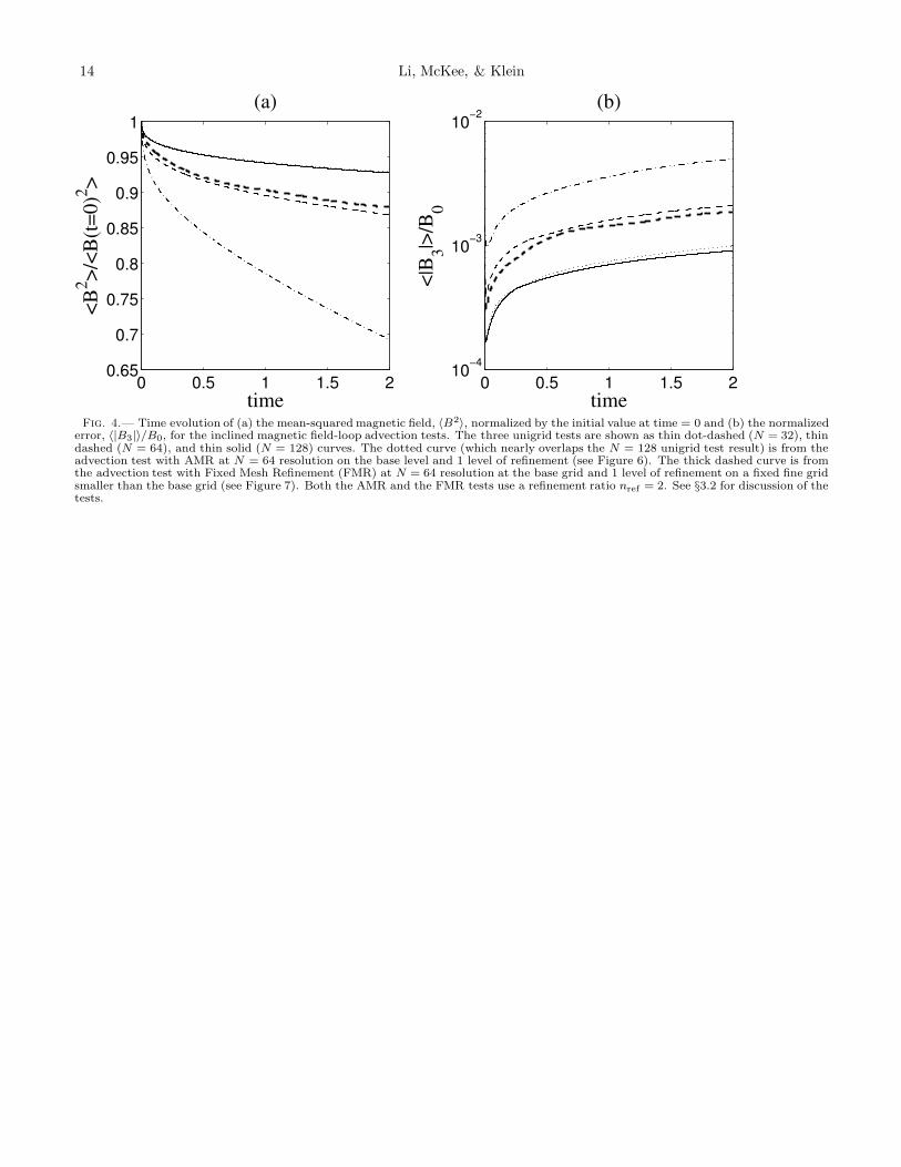
corresponding to a rotation about the y-axis. The den-sity (ρ = 1) and pressure (P = 1) are uniform and thewhole region is advected with a velocity (2,1,1). There-fore, after one unit of time, a loop starting in the middleof the rectangular region will travel across the 3D diag-onal of the box and return back to the initial position.The advection continues for 2 cycles and the images ofthe magnetic field loop at the beginning and the end ofthis test are shown in Figure 3. The top part of thefigure shows the simpler case in which the field loop isaligned with the z-axis, which is similar to a 2D advec-tion test. The loops diffuse slightly but maintain theirshapes nicely after 2 cycles of advection. The time evolu-tion of the volume mean δB2/B2 is similar to that of the3D inclined field-loop test, and Bz remains zero to themachine accuracy. In the rest of this section, we focuson the 3D inclined field-loop test results. We have per-formed the inclined field-loop test 3 times on a single levelgrid (unigrid) with 3 different resolutions: N = 32, 64and 128, as in Gardiner & Stone (2008). No AMR isused. The time evolution of the mean square field, 〈B2〉,normalized by the initial value, 〈B2

i 〉, of the whole ad-vection sequence is shown in Figure 4a as the three thincurves. The results are similar to those of Gardiner &

MHD Turbulence Resolution and Refinement Study with AMR 5

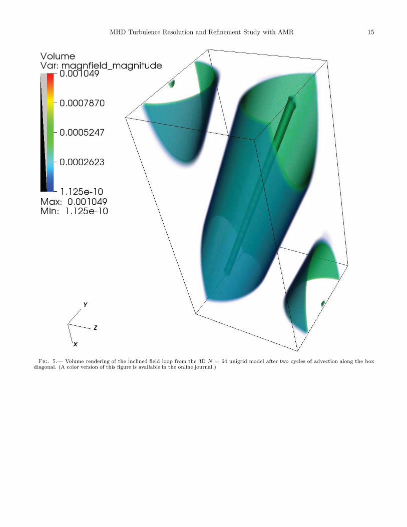
Stone (2008), who used a second-order PLM reconstruc-tion scheme, and to those of Fromang et al. (2006), whoused a second-order TVD scheme for the Ramses code.Gardiner & Stone (2008) pointed out that with the axisof the field loop aligned along an inclined direction withrespect to the computational grid, preserving B3 to bezero is non-trivial. The time evolution of the normalizederror, < |B3| > /B0, of the 3 tests is shown in Figure4b; the error is slightly smaller than that in Gardiner &Stone (2008). Figure 5 shows the volume rendering ofthe inclined field loop from the N = 64 unigrid modelafter 2-cycles of advection along the 3D box diagonal.

We next investigate how AMR affects this test. In Fig-ure 6, we show an AMR advection test with a base gridof resolution N = 64 and one level of refinement, with arefinement ratio nref = 2. The refinement criterion is onthe jump in the normalized magnetic pressure (δB2/B2),and the refinement threshold is 2.8. With this refinementcriterion, the entire field loop is covered by the fine grid.The level 1 fine grids continually move with the loop. Af-ter 2 cycles, the loop maintains its shape as in the advec-tion test on a unigrid with a resolution of N = 128. Thedotted curve in Figure 4a almost exactly coincides withthe thin solid curve. The normalized error 〈|B3|〉/B0 isalso close to that of N = 128 test.

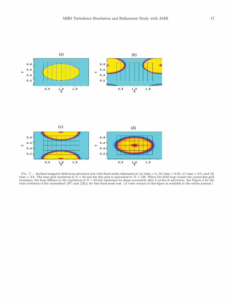
In Figure 7, we show an advection test using fixed meshrefinement (FMR) as opposed to adaptive mesh refine-ment (AMR). The level 1 fixed fine grid, which also hasnref = 2, is smaller than the base grid in space, and there-fore the loop passes through the coarse-fine grid bound-ary during the advection. The loop maintains its shapenicely after 2 cycles of advection passing in and out ofthe fine grid, but it diffuses slightly after the first pas-sage through the coarse/fine boundary. The normalizedvalues of 〈B2〉 and 〈|B3|〉 are shown in Figure 4a and4b (thick dashed curve). Note that this test also high-lights the need for effective refinement criteria and foradaptive refinement that follows the solution, since thistest only results in comparable accuracy to the uniformcoarse mesh. In the unigrid, AMR and FMR tests, ∇ · Bvanishes to order 10−16 (machine accuracy).

4. SUPERSONIC ISOTHERMAL MHD TURBULENCE WITHAMR

4.1. Simulation Model Parameters

In this section, we investigate the effects of AMR onideal MHD simulations of isothermal, supersonic turbu-lence in a strong magnetic field. We discuss only theeffects of AMR on the velocity power spectrum, the den-sity PDF, and the turbulent dissipation rate. We presentthe results of 10 simulations, all with an rms 3D sonicMach number Mrms = 10 and an initial value of theplasma β paramater β0 = 0.1; the corresponding initiialAlfven Mach number is MA,0 =

√5. Periodic boundary

conditions are used. We implemented an algorithm fordriving the turbulence with AMR using the recipe dis-cussed in Mac Low (1999). The high value of the sonicMach number and the low value of β0 have proven to bevery challenging in the past since the simulation can be-come unstable within or soon after one dynamical cross-ing time, especially with AMR. We define the dynamicalcrossing time as the length of the box divided by the rmsvelocity of the turbulent box. The driving pattern weuse is the same for all 10 models to facilitate direct com-

parison. The system is continuously driven at the largestscales, k = 1 ∼ 2, so as to maintain Mrms = 10 for 3dynamical crossing times (i.e., 0.3 sound crossing times).We analyze the data only after the first crossing time soas to allow the system to relax to a steady state. Thereare a total of 50 data files written out from each modelin the last two dynamical crossing times.

We have explored different interpolation schemes andRiemann solvers in order to determine a combinationof these algorithms which provides accuracy and stabil-ity for driven turbulence over several dynamical crossingtimes. Here we describe the combination of algorithmswe adopted for our tests:

1) The second-order accurate in space, piecewise to-tal variation diminishing (TVD) linear interpola-tion scheme described in Toro (1999).

2) The multi-dimensional shock flattening strategydeveloped by Mignone (2005), in which the interpo-lation reverts to the minmod limiter and the fluxesare computed using the HLL solver when a strongshock is detected. This provides additional dissi-pation in the proximity of a strong shock so as toguarantee positivity of the pressure.

3) The harmonic mean limiter of van Leer (1974).

4) With the CT scheme, the electromotive force(EMF) is computed at the zone edges using a twodimensional Riemann solver based on a four-stateHLL flux function (Londrillo & del Zanna 2004;Mignone et al. 2007).

5) The simple three-state HLLD approximate Rie-mann solver for the isothermal case described byMignone (2005). The absence of the entropy modein the isothermal case leads to a different formu-lation based on a three-state representation ratherthan the four-state representation of Miyoshi & Ku-sano (2005). The MHD module can also handle anon-isothermal ideal gas, but we do not includetests with non-isothermal turbulence here.

6) The characteristic tracing scheme of Colella &Woodward (1984).

We have tried the Roe solver (Roe 1986), which is anapproximate linear Riemann solver, with the above com-bination, and it is equally stable for long-duration driventurbulence simulations. The standard tests in Mignoneet al. (2007) show that the Roe and HLLD solvers yieldcomparable accuracy, but the HLLD solver is faster. Ourtests lead to the same conclusion, so we use the HLLDsolver for all the driven MHD turbulence simulations inthis investigation.

To push this stable scheme further, we carried out twosimulations on a 1283 base grid with 2 levels of refinementfor 3 dynamical crossing times: (1) Mrms = 10, plasmaβ0 = 0.02; and (2) Mrms = 17.32, plasma β0 = 0.00667.We found that the former test is stable using a CFLnumber of 0.4 and the latter test is stable using a CFLnumber of 0.35. The results for the second test (Model11) are shown with the other 10 models for reference,even though the initial conditions of this test are dif-ferent. All the standard tests shown in §3 use the above

6 Li, McKee, & Klein

combination of algorithms and demonstrate the accuracyresulting from this choice. However, it must be bornein mind that our choice of Riemann solver, reconstruc-tion, limiter, and EMF averaging schemes is probably notunique, since we have tested only a small combination ofall existing solvers and reconstruction schemes.

We have also tried the third-order accurate Piecewise-Parabolic-Method (PPM) of Colella & Woodward (1984)as the reconstruction scheme, but the simulation be-comes unstable within or soon after one dynamical cross-ing time, regardless of what limiter is used (even with themost diffusive minmod limiter). We conclude that spe-cial treatments will be required to use higher-order inter-polation schemes for simulations of high Mach number,strong magnetic field turbulence.

4.2. Refinement Criteria

Kritsuk et al. (2006) have proposed two refinementcriteria for hydrodynamic turbulence, one based on thejump in pressure and one on the norm of the velocity gra-dient matrix. We have used this as a guideline in settingour refinement criteria for MHD turbulence. For the firstcriterion, we replace the thermal pressure P by the sumof the thermal and magnetic pressures, Ptot = P+B2/8π;cells are tagged for refinement if ∆Ptot/Ptot exceeds apre-determined threshold. For the second criterion weuse the Kritsuk et al. (2006) refinement criterion forstrong shear, which is determined by computing the normof the velocity gradient matrix ‖∂ivj‖ without the con-tribution from the diagonal elements. The norm is thennormalized by cs/∆x and is tagged for refinement at athreshold that is the same as that for the total pres-sure jump. Kritsuk et al. (2006) found that AMR resultsagreed well with unigrid results at the maximum reso-lution of the AMR for a pressure jump threshold of 2.With the inclusion of the shear velocity refinement crite-rion, they found that the pressure jump threshold couldbe raised to 3.

We have carried out a series of tests to investigatethe sensitivity to the refinement threshold. Unlike Krit-suk et al. (2006), we find that a refinement threshold∆Ptot/Ptot = 2 causes the base level to be completelyrefined in all our AMR models, most likely because ofthe inclusion of magnetic pressure. Kritsuk et al. (2006)

use an AMR refinement ratio n`−1ref = 4. For example,

their 10243 AMR run has a base grid of 2563 with onelevel of refinement. All of our tests use n`−1

ref = 2, exceptfor one with n0

ref = 4 for comparison. With a refinementratio of 2, two levels of refinement are needed to achievea maximum resolution of 10243 with a 2563 base grid.The fraction of the volume covered by the first level ofrefinement (i.e., the “coverage”) is independent of therefinement ratio. Thus, the coverage at level 1 with arefinement ratio of 2 (maximum refinement equivalent to5123) is the same as that at level 1 with a refinement ra-tio of 4 (10243), but the number of cells is 8 times largerin the latter case. The coverage at level 2 with a refine-ment ratio of 2 (10243) is smaller than that of level 1with a refinement ratio of 4, and the number of cells iscorrespondingly smaller.

A simple way of characterizing the refinement of a mul-tilevel AMR calculation is the volume-averaged resolu-

tion,

〈R〉 ≡∑

i

RiVi. (3)

where Ri is the 1D resolution of level i and Vi is thefractional volume coverage for level i excluding higherlevels. For example, for Model 4, the volume coverage oflevels 0, 1 and 2 is Vi = 0.35, 0.48, 0.17, respectively (thetotal level 1 coverage is 0.65 but V1 excludes the volumerefined at level 2). For this model, 〈R〉 = 128 × 0.35 +256×0.48+512×0.17 = 255, which is very close to thatof a 2563 unigrid model.

We have performed a large number of ideal MHD tur-bulent box experiments using different base grid sizes(1283 and 2563), different refinement criteria, differentminimum block sizes, and different refinement ratios. Wealso have two unigrid turbulence models, at 1283 and5123, for comparison. The unigrid 5123 model will serveas the reference for all AMR models presented in thispaper.

4.3. Power Spectrum

In this section, we study how changes in resolutionand refinement criteria affect the velocity power spec-trum, Pv(k) ∝ k−n, in terms of the power index, n,and the extent of the inertial range, kmax. We fit thepower spectra obtained from the 50 data dumps between1 and 3 dynamical crossing times between k = 4 (to avoidthe effects of driving) up to a value of k that increasesby unity at each iteration. All the fitting results andthe plots shown in section 4 are time-averaged resultsfrom the 50 data dumps over these two dynamical cross-ing times. (Since the turbulence remains correlated forabout one dynamical crossing time (e.g. Li et al. 2008),we assign an error to the mean value of P (k) from the50 data dumps equal to the standard deviation dividedby

√3.) As more points are added, the uncertainty in

the slope decreases, and correspondingly so does the re-duced χ2 of the fit. However, the reduced χ2 begins toincrease when the power spectrum turns over due to nu-merical dissipation; we define the point at which χ2 is aminimum as the upper end of the inertial range, kmax.In order to overcome the possibility that noise in thedata could artificially lower kmax, we omit the point atkmax + 1 that led to the increase in χ2 and evaluate thereduced χ2 of the fit including the point at kmax + 2;if the value of the reduced χ2 is less than the previousminimum, we set kmax = kmax(previous)+2 and proceedwith the iteration. We allow for the possibility that thenoise fluctuation could be up to three cells wide. Thisprocedure allows our estimate of the inertial range toextend beyond the bumps at k ' 9 that are apparentin the spectra in Figure 8 and are due to an artifact inthe driving pattern. This method is conservative, butit can eliminate the impact of the bottleneck effect ondetermining the spectral index or the size of the inertialrange (e.g. Verma 2007; Kritsuk et al. 2007) when theinertial range available for turbulent energy transfer issmall. However, we note that our MHD turbulence testsdo not suffer from the bottleneck effect.

In Table 1, we present the fitted results of the 10 idealMHD turbulence models. The table includes the refine-ment coverage at each fine level. For example, in Model4, level ` = 1 has a volumetric coverage of 65% of the

MHD Turbulence Resolution and Refinement Study with AMR 7

computational domain and level 2 has a volumetric cover-age of 17% of the computational domain (or 17/65 ∼ 26%of level 1). In Figure 8, the compensated power spectraof models 1, 3, 4, 6, and 10 are shown. We summarizethe results in Figure 8 and Table 1 as follows:

1) Models 1 and 10 are unigrid simulations and pro-vide a basis for evaluating the AMR models. Thespectral index of Model 10 is n = 1.42± 0.02, con-sistent with other strong magnetic field supersonicturbulence simulations, which show that the powerspectrum is close to the Iroshnikov-Kraichnan spec-trum (Iroshnikov 1963; Kraichnan 1965). The lowresolution Model 1 has a steeper spectral index,n = 1.75 ± 0.06. We repeated Model 10 (uni-grid 5123 with an HLLD solver) using the Roesolver and obtained a power spectrum that agreesto within the uncertainty of fitting.

2) Models 2 to 4 test the effect of changing the refine-ment threshold for the total pressure jump from3.25 to 2.5. As the threshold drops, the refinementcoverage increases, and the spectral index slowlyapproaches that of Model 10. Correspondingly,the inertial ranges are significantly longer (2 times)than in Model 1 and appear to converge to that ofModel 10 as the refinement coverage increases.

3) Model 5 tests the effect of shear flow refinementon the AMR calculation. There is no noticeableincrease in the accuracy of Model 5 compared toModel 4, presumably because the additional cri-terion did not significantly increase the averagerefinement. Model 8 has shear flow refinement,whereas Model 7 does not; however, Model 8 has 2levels of refinement compared to 1 for Model 7, sono inference on the effect of the shear flow refine-ment can be drawn.

4) Comparison of models 5 and 6, and of models 4and 7, addresses the effects of refinement coverageon the overall improvement of the power spectrum.Model 6 has only 1 level of refinement but uses arefinement ratio of 4, equivalent to full coverageof level 1 at the resolution of level 2 in Model 5,which is a 2-level model using a refinement ratio of2. The average refinement in Model 6 is about 60%greater than in Model 4; correspondingly, there isa substantial improvement to the power spectrumand a modest increase in the size of the inertialrange. However, the computational time for Model6 is about 3 times that of Model 5, a big price topay for the improvement. The reason for the largeincrease in computing time is that each cell thatis refined only to level 1 in the two-level run has8 times as many refined cells in the one-level run.An additional test of the effects of refinement cov-erage is provided by comparing Model 7 to Model4; the former uses a base grid of 2563 and only 1level of refinement. Model 7 has an average refine-ment about 20% greater than Model 4. For this,one gets a significant improvement in the spectralindex, but only a small increase in the size of theinertial range. The computation time for Model 7is similar to that for Model 6.

5) Like Models 2-4, Models 8 and 9 address the im-plications of increased refinement coverage for im-provements in the power spectrum. Note that thelevel 2 resolution in these models is the same asthat in a 10243 resolution simulation. Model 9has only a slightly lower threshold for the pressurejump than Model 8 (2.3 vs. 2.5), but this leadsto almost a twofold increase in the average refine-ment. This increase in average refinement yieldsan increase in the inertial range, but has no signifi-cant effect on the spectral index. Even though theaverage refinement of Model 9 exceeds that in theunigrid Model 10, the latter appears to have themost accurate spectral index and the largest iner-tial range. Our finding that a unigrid simulation at5123 resolution is superior to an AMR simulationwith a maximum refinement of 10243 is consistentwith the conclusion of Kritsuk et al. (2006) that alarge base grid is required to obtain the advantagesof AMR for simulations of turbulence.

6) Model 11 has different initial conditions from theabove 10 models. This model has Mrms = 17.32and plasma β0 = 0.00667; the correspondingAlfven Mach number is MA,0 = 1. This model is inmany ways similar to Model 3 in Table 1 in termsof the power spectral index, the length of inertialrange, and refinement coverage, although Model 3has very different initial conditions (Mrms = 10,

β0 = 0.1, and MA,0 =√

5).

From the above summary, we can see that changes in re-finement criteria directly affect the average refinement,which in turn directly affects the quality of the turbu-lence power spectrum.

In Figure 9, we show the power spectra of the magneticfield for models 1, 3, 4, 6, and 10. The convergencebehavior of the magnetic field power spectrum is similarto that of the velocity power spectra in Figure 8.

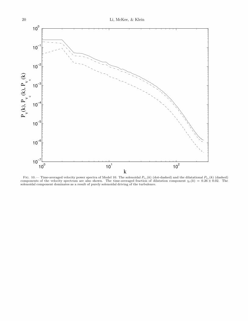
A recent study of the effects of purely solenoidal andpurely compressive turbulent driving (Federrath et al.2010) shows that there are significant differences in theturbulence statistics between these two extreme driv-ing models. For example, the dispersion in the den-sity PDF with purely compressive driving can be 3times that resulting from purely solenoidal driving. Forpurely solenoidal driving, the solenoidal component ofthe power spectrum will dominate the dilatational com-ponent. This is reversed for purely compressive driv-ing. Reality probably is somewhere in between thesetwo extreme cases. Our driving is purely solenoidal. Wedecompose the solenoidal (∇ · vs ≡ 0) and dilatational(∇×vc ≡ 0) components from the velocity, v = vs +vc,by

vc(k)= [k · v(k)]k (4)

vs(k)= [k× v(k)] × k (5)

(Lemaster & Stone 2009). We define the fraction of thedilatational component in the velocity power spectrumas

χc(k) ≡ Pvc(k)

Pv(k)(6)

(Kritsuk et al. 2009a). Figure 10 shows the time-averaged velocity power spectrum of Model 10 with

8 Li, McKee, & Klein

the solenoidal and dilatational components. The time-averaged χc(k) = 0.27±0.01, 0.26±0.01, and 0.26±0.02for Models 1, 4, and 10, respectively. It appears thatχc(k) is not sensitive to the resolution. For Model11, which has a smaller Alfven Mach number, χc(k) =0.27 ± 0.02 is the same. The value of χc(k) in an idealMHD turbulence model with purely solenoidal forcing(Kritsuk et al. (2009a)) is ≈ 1/4, similar to our values.Lemaster & Stone (2009) measure the dilatational com-ponent of the kinetic energy (i.e., the density-weightedvelocity power spectrum) and find that it is even smallercompared to the solenoidal component.

4.4. Density PDF

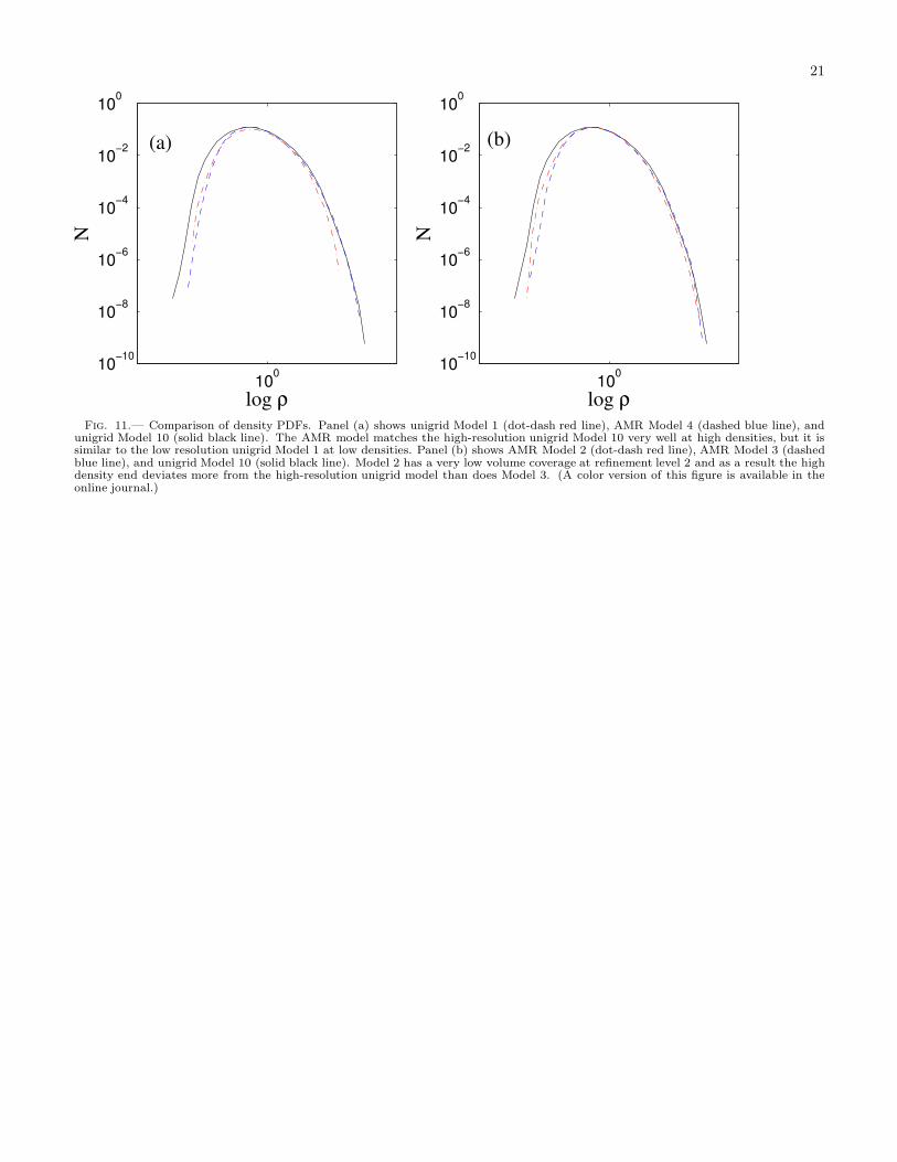
In Figure 11a, we show the probability density func-tions (PDFs) of density for models 1, 4, and 10 todemonstrate the effect of refinement on the density PDFin AMR simulations. The density PDF of the unigridModel 1 at 1283 resolution is narrower than the densityPDF of the unigrid Model 10 at 5123 resolution. A lowresolution unigrid turbulence simulation cannot reach thehighest and lowest densities attainable in a high resolu-tion unigrid simulation. As a result, the maximum wavespeed in a low resolution simulation can be lower than ina high resolution simulation, since the minimum densityis higher and the maximum Alfven velocity is most likelysmaller. On the other hand, since the maximum densityin a low resolution simulation is smaller, the clump massfunction will be reduced at high densities; this could beproblematic in simulations of star formation.

AMR offers the best of both worlds: As shown in Fig-ure 11a, at low densities the AMR simulation (Model 4)is close to Model 1 and therefore does not have the veryhigh Alfven velocities that appear in the high resolutionModel 10. In simulations of star formation, the loss ofresolution at low densities is not important. However,Model 4 has the same maximum resolution as Model 10,and the AMR enables it to track accurately the high-density portion of the density PDF, which is critical insimulations of star formation.

In Figure 11b, the density PDFs of models 2 and 3are plotted on top of the density PDF of Model 10. Thehigh-density part of the PDF of Model 2 deviates morefrom that of Model 10 than that of Model 3 because ofthe very low level 2 coverage (1.3%) in Model 2. Model 3suggests that in order to have a good match to the highdensity part of the Model 10 PDF, the level 2 coveragemust be & 10% for this problem. With the Roe solver,the PDF of a unigrid simulation extends to slightly lowerdensities than that for the same unigrid simulation usingthe HLLD solver, but the high-density parts of the PDFare almost the same. Therefore, not only is the Roesolver slower than HLLD solver per time step, but thetime step in an MHD turbulence simulation will also besmaller.

4.5. Turbulent Energy Dissipation Rate

Both hydrodynamic and MHD turbulence simulationsshow that turbulence decays on the order of a dynami-cal crossing time. The dissipation rate of the turbulentenergy is of order ρv3

rms/L. Specifically, we write

E = ερv3

rms

Lint, (7)

where vrms is the density-weighted rms velocity of theturbulence and the integral length scale (Batchelor 1953)for a compressible fluid with a magnetic field is definedby

Lint =3π

2〈ρv2 + B2/4π〉

∫

k−1Etot(k)dk, (8)

where Etot(k) is the total energy power spectrum, in-cluding both kinetic energy and magnetic energy. Su-personic MHD turbulence simulations (Mac Low (1999),Stone et al. (1998), and Lemaster & Stone (2009)) sug-gest that the proportionality constant ε ∼ 0.5. Kaneda etal. (2003) summarized the results of many pure hydrody-namic incompressible simulations and showed that, withtheir highest resolution (40963) simulation, ε convergedto about 0.4.

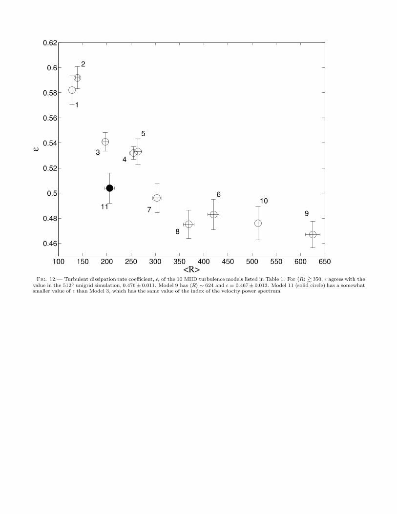
The turbulent dissipation rate coefficient ε for the 10models presented here is plotted as a function of the av-erage resolution in Figure 12. The horizontal uncertaintybar is obtained from the standard deviation of the vari-ation of the refinement coverage during the simulation,usually a few percent of the refinement coverage. Mod-els 1 and 10 do not have horizontal error bars since theyare unigrid models. Figure 12 shows that the dissipa-tion rate is within the uncertainties of the 5123 unigridsimulation for 〈R〉 & 350. For the three AMR mod-els with 〈R〉 & 350, the mean ε = 0.48 ± 0.02, whichagrees well with the result from the 5123 unigrid model,ε = 0.48 ± 0.01, and is similar to the results from otherunigrid simulations of ideal MHD turbulence, ε ' 0.5(e.g. Lemaster & Stone 2009). In Figure 12, we also plotthe value of ε for Model 11 (solid circle) for reference.Although this model has the same spectral index for thevelocity power spectrum as Model 3, the value of ε of thismodel is smaller.

Models 6, 8, and 9 have similar turbulent dissipationrates as Model 10, and one might think that using a lowerresolution base grid with AMR would have the advantageof reaching the dissipation rate obtained from a unigridmodel with higher resolution. However, Table 1 showsthat the CPU usage for these 3 models actually is higherthan for the unigrid Model 10. This is another indicationof the inefficiency of AMR for turbulence studies until amuch larger base grid is used.

4.6. Turbulent Magnetic Field

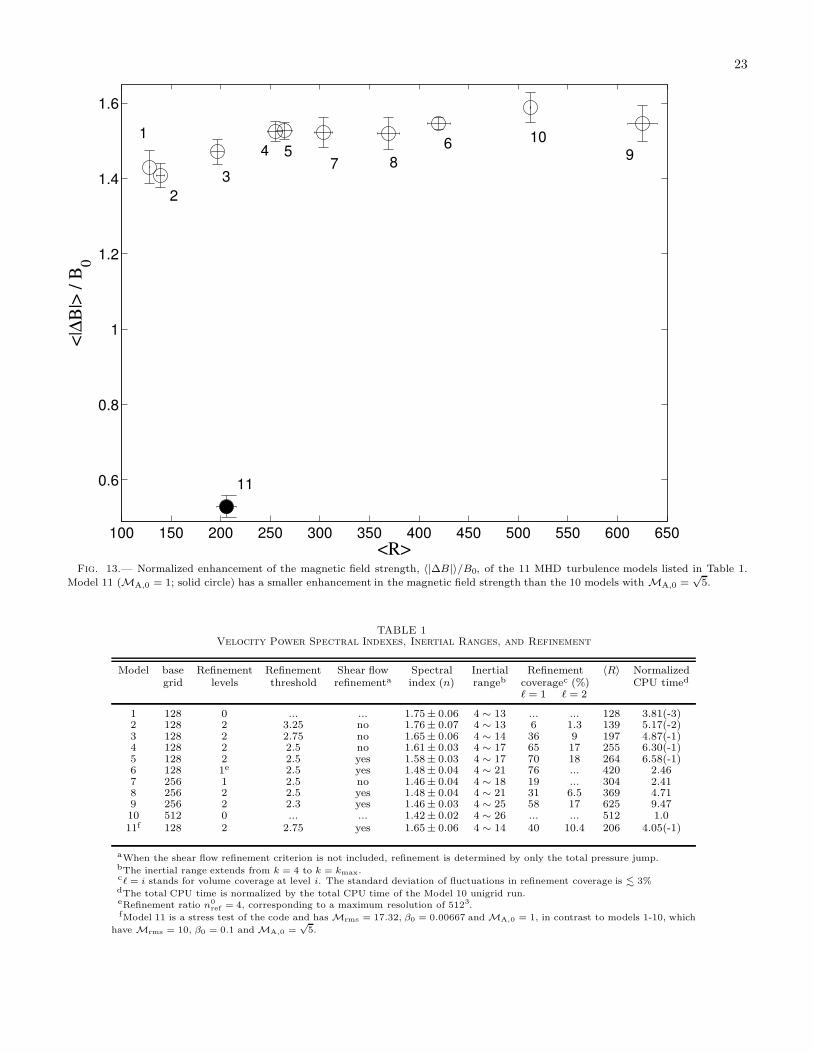
For a magnetized turbulent system, the magnetic fieldstrength will be enhanced as the result of field-linestretching. The maximum field-line stretching will belimited by the grid resolution, which determines the nu-merical diffusion of the magnetic field that we want tominimize. We plot the time-averaged change in mag-netic field strength, 〈|∆B|〉, normalized by the initialmean field strength, B0, versus the volume-averagedresolution 〈R〉 in Figure 13. Since the initial Alfven

Mach number is modest (MA,0 =√

5) for Models 1-10, the enhancement of the field strength is also modest,〈|∆B|〉 ∼ (1.54±0.09)B0 from the mean value from Mod-els 6 to 10, which have overlapping error bars and whichhave 〈R〉 & 300. The value of 〈|∆B|〉/B0 = 0.53 forModel 11 is smaller since MA,0 = 1 is smaller. Only sys-tems with initially high Alfven Mach numbers can havea turbulent magnetic field many times greater than themean field, and simulations of such systems require much

MHD Turbulence Resolution and Refinement Study with AMR 9

higher resolution to have converged magnetic field statis-tics (e.g. Kritsuk et al. 2009a).

5. CONCLUSIONS AND DISCUSSIONS

We have developed a robust MHD module for our newAMR code, ORION2, and have demonstrated its abilityto carry out accurate long-duration AMR simulations ofhighly supersonic turbulent flows with strong magneticfields (β � 1, MA ∼ 1). Although unigrid simulationsof such flows have been published (e.g., Kritsuk et al.2009b), to our knowledge the AMR simulations of theseflows presented herein are the first to appear in the litera-ture. Since observations suggest that GMCs have highlysupersonic flows with relatively strong magnetic fields(McKee & Ostriker 2007) and since AMR is essential forfollowing gravitational collapse, this represents an impor-tant advance in our ability to study the conditions thatlead to star formation. ORION2 is able to do this be-cause the code is sufficiently flexible that one can easilyexperiment with different reconstruction schemes, Rie-mann solvers, CT EMF averaging schemes, and limitersto find the suitable combination that we have described.

We have tested the accuracy of our code with sev-eral standard MHD tests, including the Ryu & Jones(1995) shock tube test, the Brio & Wu (1988) shock tubetest, and the 3D current-loop test on unigrid, FMR, andAMR. The results we have presented here demonstratethat the CTU+CT algorithm performs accurately andworks properly within the Chombo AMR framework.We found that the piecewise linear, spatially second-order, TVD scheme combined with a multi-dimensionalshock flattening strategy developed by the PLUTO group(Mignone et al. 2007) can work with both Roe and HLLDsolvers to enable stable, long-duration (3 crossing times)simulations of driven MHD turbulence with an rms Machnumber of Mrms = 17.3 and an initial plasma β param-eter of β0 = 0.0067 on a 1283 base grid with 2 levels ofrefinement.

We examined the velocity power spectrum, the densityPDF, and turbulent dissipation rate in our investigationof the effectiveness of AMR on the quality of MHD turbu-lence simulations. By varying the refinement criteria, thebase grid resolution, and the number of refinement levels,we find that the quality of the turbulence statistics—inparticular, the spectral index of the velocity power spec-trum and the extent of the inertial range—is more closelyrelated to the average refinement coverage than to themaximum level of refinement. Analysis of the densityPDFs shows that, with our refinement criteria, AMR isparticularly powerful for simulations in which interest isfocused on the regions of highest density: it does notcapture the regions of the lowest density as well as aunigrid simulation, but it does capture the PDF of thehigh-density regions quite accurately (e.g. Collins et al.2011). Our result for the dissipation coefficient for tur-bulence with M = 10 and β0 = 0.1 is ε = 0.48 ± 0.01.This is consistent with other numerical studies of MHDturbulence with unigrid codes, which find that ε ∼ 0.5.

We would like to thank Brian Van Straalen for helpingimprove the scalability performance of the AMR Imple-mentation of the MHD module of ORION2. We alsothank Christoph Fedderath, Jim Stone, Alexei Kritsukand Tom Abel for helpful discussions on the paper. Sup-port for this research was provided by NASA throughNASA ATP grant NNX09AK31G (RIK, CFM, andPSL), the US Department of Energy at the Lawrence Liv-ermore National Laboratory under contract DE-AC52-07NA 27344 (RIK), the Lawrence Berkeley National Lab-oratory under contract DE-AC02-05CH11231 (DFM),and the NSF through grant AST-0908553 (CFM andRIK). This research is also supported by an LRAC Tera-grid grant of high performance computing from the NSFand the NASA Advanced Computing (NAS) Divisionthrough a NASA ATP grant.

REFERENCES

Balsara, D. S. & Spicer, D. S. 1999, J. Comput. Phys., 149, 270Balsara, D. 2001, J. Comput. Phys., 174, 614Batchelor, G. K. 1953, Homogeneous Turbulence, Cambridge

University Press.Berger M.J., Colella, P. 1989, J. Comput. Phys., 82, 64Berthon, C. 2005, Commun. Math. Sci. 3 (2) 133Brio, M. & Wu, C. C. 1988, J. Comput. Phys., 75, 400Colella, P. 1990, J. Comput. Phys., 87, 171Colella, P., Graves, D. T., Keen, N. D., et al. 2000,

https://seesar.lbl.gov/ANAG/chombo)Colella, P. & Woodward, P. R. 1984, J. Comput. Phys., 54, 174Collins, D. C., Padoan, P., Norman, M. L., & Xu, H. 2011, ApJ,

731, 59Crockett, R. K., Colella, P., Fisher, R. T., Klein, R. I., & McKee,

C. F. 2005, J. Comput. Phys., 203, 422Crutcher, R. M. 1999, ApJ, 520, 706Dedner, A., Kemm, F., Kroner, D., et al. 2002, J. Comput. Phys.

175, 645.Evans, C. R. & Hawley, J. F. 1988, ApJ, 659Federrath, C., Roman-Duval, J., Klessen, R. S., Schmidt, W., &

Mac Low, M.-M. 2010, A&A, 512, 81Fromang, S. Hennebelle, P., & Teyssier, R. 2006, A&A, 457, 371Fryxell, B., Olson, K., Ricker, P., et al. 2000, ApJS, 131, 273Gardiner, T. A., & Stone, J. M. 2005, J. Comp. Phys., 205, 509Gardiner, T. A., & Stone, J. M. 2008, J. Comp. Phys., 227, 4123Gottlieb, S., Shu, C.-W. 1996, NASA CR-201591 ICASE Rep. 96-

50, 20 (Washington: NASA)Hayes, J. C., Norman, M. L., Fiedler, R. A., et al. 2006, ApJS, 165,

188

Iroshnikov, P. S. 1963, AZh, 40, 742 (English transl. Soviet Astron.,7, 566 [1964])

Kaneda Y, Ishihara T, Yokokawa M, Itakura K, & Uno A. 2003,Phys. Fluids, 15, L21

Klein, R. I. 1999, J. Comput. Appl. Math., 109, 123Kraichnan, R. H. 1965, Phys. Fluids, 8, 1385Kritsuk, A. G., Norman, M. L., & Padoan, P. 2006, ApJ, 638, L25Kritsuk, A. G., Norman, M. L., Padoan, P. & Wagner, R. 2007,

ApJ, 665, 416Kritsuk, A. G., Ustyugov, S. D., Norman, M. L., & Padoan, P.

2009a, J. Phys.: Conf. Ser., 180, 012020Kritsuk, A. G., Ustyugov, S. D., Norman, M. L., & Padoan,

P. 2009b, Numerical Modeling of Space Plasma Flows:ASTRONUM-2008, 406, 15

Krumholz, M. R., McKee, C. F., & Klein, R. I. 2004, ApJ, 611, 399Krumholz, M. R., Klein, R. I., McKee, C. F., & Bolstad, J. 2007,

ApJ, 667, 626Lemaster, M. N. & Stone, J. M. 2009, ApJ, 691, 1092LeVeque, R. J., Numerical Methods for Conservation Laws, second

ed., Birkhuser, Basel, Switzerland, Boston, USA, 1992.Li, P.S., McKee, C. F., & Klein, R. I. 2008, ApJ, 684, 380Londrillo, P. & del Zanna, L. 2004, J. Comput. Phys., 195, 17Mac Low, M.-M. 1999, 524, 169Mac Low, M.-M. & Klessen, R. S. 2004, Rev. Mod. Phys., 76, 125Martin, D & Colella, P. 2000, J. Comput. Phys., 163, 271Masunaga, H., Miyama, S. M., & Inutsuka, S.-I. 1998, ApJ, 495,

346McKee, C. F., & Ostriker, E. C. 2007, ARA&A, 45, 565Mignone, A. 2005, J. Comput. Phys., 225, 1472

10 Li, McKee, & Klein

Mignone, A., Bodo, G., Massaglia, S., et al. 2007, ApJS, 170, 228Mignone, A. & Tzeferacos, P. 2010, J. of Comput. Phys., 229, 2117Miyoshi, T., & Kusano, K. 2005, J. of Comput. Phys., 208, 315Wang, P. & Abel, T. 2009, ApJ, 696, 96Powell, K. G., Roe, P. L., Linde, T. J., Gombosi, T. I., & de Zeeuw,

D. L. 1999, J. Comput. Phys., 153, 284Roe, P. L. 1986, Annu. Rev. Fluid Mech., 18, 337Ryu, D. & Jones, T. W. 1995, ApJ, 442, 228Schmidt, W., Federrath, C., Hupp, M., Kern S., & Niemeyer, J. C.

2009, A&A, 494, 127Stone, J. M., Gardiner, T. A., Teuben, P., Hawley, J. F., & Simon,

J. B. 2008, ApJ, 178, 137Stone, J. M., Ostriker, E. C., & Gammie, C. F. 1998, ApJ, 508,

L99Toro, E. F. 1999, Riemann Solvers and Numerical Methods for

Fluid Dynamics, (Berlin: Springer Verlag)

Toth, G. 2000, J. Comput. Phys. 161 (2000) 605.Truelove, J. K., Klein, R. I., McKee, C. F., et al. 1997, ApJ, 489,

L179Truelove, J. K., Klein, R. I., McKee, C. F., et al. 1998, ApJ, 495,

821van Leer, B. 1974, J. Comput. Phys., 14, 361Teyssier, R. 2002, A&A, 385, 337Verma, M. K. & Donzis, D. 2007, J. Physics A: Mathematical and

Theoretical, 40, 4401Waagan, K. 2009, J. of Comput. Phys., 228, 8609Waagan, K., Federrath, C. & Klingenberg, C., 2011, J. of Comput.

Phys., 230, 3331Wang, P. & Abel, T. 2009, ApJ, 696, 96Zhang, X. & Shu, C. W. 2010, J. Comput. Phys., 229, 8918

MHD Turbulence Resolution and Refinement Study with AMR 11

0 0.5 1

1

2

3

4ρ

0 0.5 1

0

50

100

150

P

0 0.5 1

50

100

150

200

250

E

0 0.5 1

−10

−5

0

5

10

vx

0 0.5 1−0.5

0

0.5

vy

0 0.5 1−0.5

0

0.5

vz

0 0.5 11

1.5

2

Bx

0 0.5 10

2

4

6

By

0 0.5 1−0.5

0

0.5

Bz

Fig. 1.— One of the Ryu & Jones (1995) shock-tube test results using the ORION2 MHD module. The top row, from left to right, showsthe density (ρ), pressure (P ), total energy density (Etot) along the shock tube, which is resolved by 512 cells. The second row shows thethree components of velocity and the bottom row shows the three components of magnetic field. In these panels, from left to right, we cansee the fast shock, slow rarefaction (apparent in the plots of vy and By), contact discontinuity, slow shock, and fast shock.

12 Li, McKee, & Klein

0 0.5 10

0.2

0.4

0.6

0.8

1

ρ

0 0.5 10

0.2

0.4

0.6

0.8

1

P0 0.5 1

−0.4

−0.2

0

0.2

0.4

0.6

0.8

vx

0 0.5 1

−1.5

−1

−0.5

0

vy

0 0.5 10.5

1

1.5

2

T

0 0.5 1

−1

−0.5

0

0.5

1

By

Fig. 2.— Brio & Wu (1988) shock tube test results. The top row, from left to right, shows the density (ρ), pressure (P ), and velocityalong the shock tube (vx). The second row shows the y-component of the velocity (vy), the temperature (T ), and the y-component of themagnetic field (By). The shock tube is resolved by 800 cells. A compound wave composed of an Alfven and a slow wave is seen as thespike near the middle of the figure.

MHD Turbulence Resolution and Refinement Study with AMR 13

Fig. 3.— Vertical magnetic field-loop advection test on a unigrid with resolution N = 64 (a) at the beginning of the advection and(b) after 2 cycles of advection. The inclined magnetic field loop, which is rotated by 63.4◦ about the y-axis from the vertical, (c) at thebeginning of the advection and (d) after 2 cycles of advection. Both field loops are advected with velocity (2,1,1). All four panels are atz=0.5. The field loops maintain their shapes accurately after 2 cycles of advection. (A color version of this figure is available in the onlinejournal.)

14 Li, McKee, & Klein

0 0.5 1 1.5 20.65

0.7

0.75

0.8

0.85

0.9

0.95

1

time

<B

2>

/<B

(t=

0)2

>(a)

0 0.5 1 1.5 210

−4

10−3

10−2

(b)

time

<|B

3|>

/B0

Fig. 4.— Time evolution of (a) the mean-squared magnetic field, 〈B2〉, normalized by the initial value at time = 0 and (b) the normalizederror, 〈|B3|〉/B0, for the inclined magnetic field-loop advection tests. The three unigrid tests are shown as thin dot-dashed (N = 32), thindashed (N = 64), and thin solid (N = 128) curves. The dotted curve (which nearly overlaps the N = 128 unigrid test result) is from theadvection test with AMR at N = 64 resolution on the base level and 1 level of refinement (see Figure 6). The thick dashed curve is fromthe advection test with Fixed Mesh Refinement (FMR) at N = 64 resolution at the base grid and 1 level of refinement on a fixed fine gridsmaller than the base grid (see Figure 7). Both the AMR and the FMR tests use a refinement ratio nref = 2. See §3.2 for discussion of thetests.

MHD Turbulence Resolution and Refinement Study with AMR 15

Fig. 5.— Volume rendering of the inclined field loop from the 3D N = 64 unigrid model after two cycles of advection along the boxdiagonal. (A color version of this figure is available in the online journal.)

16 Li, McKee, & Klein

Fig. 6.— Inclined magnetic field-loop advection test with AMR at the beginning of the advection (left panel) and after 2 cycles ofadvection (right panel). The blocks surrounding the loop show the location of the fine grids. Although the base grid has a resolution ofN = 64, the loop is always refined at a resolution of N = 128. The time evolution of the normalized 〈B2〉 and 〈|B3|〉 is almost the same asthat of a unigrid N = 128 test (Fig. 4). (A color version of this figure is available in the online journal.)

MHD Turbulence Resolution and Refinement Study with AMR 17

Fig. 7.— Inclined magnetic field-loop advection test with fixed mesh refinement at (a) time = 0, (b) time = 0.25, (c) time = 0.5, and (d)time = 2.0. The base grid resolution is N = 64 and the fine grid is equivalent to N = 128. When the field loop crosses the coarse-fine gridboundary, the loop diffuses to the resolution of N = 64 but maintains its shape accurately after 2 cycles of advection. See Figure 4 for thetime evolution of the normalized 〈B2〉 and 〈|B3|〉 for this fixed mesh test. (A color version of this figure is available in the online journal.)

18 Li, McKee, & Klein

100

101

102

10−2

10−1

100

k

Pv (

k)

k1.4

2

1

3

4

610

Fig. 8.— Compensated velocity power spectra of models 1, 3, 4, 6, and 10. The spectra are compensated by k1.42, the spectral indexof the unigrid 5123 Model 10. Models 3, 4, and 6 are simulations with AMR. Models 1 and 10 have just the base grid at 1283 and 5123,respectively. The spectra are labeled by their model numbers. The horizontal line is provided to aid comparison of the inertial ranges ofall the models. See §4.3 for a discussion of how refinement coverage affects the inertial range. (A color version of this figure is available inthe online journal.)

MHD Turbulence Resolution and Refinement Study with AMR 19

100

101

102

10−6

10−5

10−4

10−3

10−2

10−1

100

k

PB

(k)

106431

Fig. 9.— Magnetic field power spectra of models 1, 3, 4, 6, and 10 (with model numbers shown in the same order as the curves, startingfrom bottom) without compensation. The spectra show a similar convergence behavior with resolution as the velocity spectra in Figure 8.(A color version of this figure is available in the online journal.)

20 Li, McKee, & Klein

100

101

102

10−7

10−6

10−5

10−4

10−3

10−2

10−1

100

k

Pv(k

), P

vc(k

), P

vs(k

)

Fig. 10.— Time-averaged velocity power spectra of Model 10. The solenoidal Pvs(k) (dot-dashed) and the dilatational Pvc

(k) (dashed)components of the velocity spectrum are also shown. The time-averaged fraction of dilatation component χc(k) = 0.26 ± 0.02. Thesolenoidal component dominates as a result of purely solenoidal driving of the turbulence.

MHD Turbulence Resolution and Refinement Study with AMR 21

100

10−10

10−8

10−6

10−4

10−2

100

log ρ

N

100

10−10

10−8

10−6

10−4

10−2

100

log ρ

N

(a) (b)

Fig. 11.— Comparison of density PDFs. Panel (a) shows unigrid Model 1 (dot-dash red line), AMR Model 4 (dashed blue line), andunigrid Model 10 (solid black line). The AMR model matches the high-resolution unigrid Model 10 very well at high densities, but it issimilar to the low resolution unigrid Model 1 at low densities. Panel (b) shows AMR Model 2 (dot-dash red line), AMR Model 3 (dashedblue line), and unigrid Model 10 (solid black line). Model 2 has a very low volume coverage at refinement level 2 and as a result the highdensity end deviates more from the high-resolution unigrid model than does Model 3. (A color version of this figure is available in theonline journal.)

22 Li, McKee, & Klein

100 150 200 250 300 350 400 450 500 550 600 650

0.46

0.48

0.5

0.52

0.54

0.56

0.58

0.6

0.62

<R>

ε

10

9

8

6

5

4

3

2

7

1

11

Fig. 12.— Turbulent dissipation rate coefficient, ε, of the 10 MHD turbulence models listed in Table 1. For 〈R〉 & 350, ε agrees with thevalue in the 5123 unigrid simulation, 0.476± 0.011. Model 9 has 〈R〉 ∼ 624 and ε = 0.467± 0.013. Model 11 (solid circle) has a somewhatsmaller value of ε than Model 3, which has the same value of the index of the velocity power spectrum.

MHD Turbulence Resolution and Refinement Study with AMR 23

100 150 200 250 300 350 400 450 500 550 600 650

0.6

0.8

1

1.2

1.4

1.6

<R>

<|∆

B|>

/ B

0

11

10

98

6

754

1

2

3

Fig. 13.— Normalized enhancement of the magnetic field strength, 〈|∆B|〉/B0, of the 11 MHD turbulence models listed in Table 1.

Model 11 (MA,0 = 1; solid circle) has a smaller enhancement in the magnetic field strength than the 10 models with MA,0 =√

5.

TABLE 1Velocity Power Spectral Indexes, Inertial Ranges, and Refinement

Model base Refinement Refinement Shear flow Spectral Inertial Refinement 〈R〉 Normalizedgrid levels threshold refinementa index (n) rangeb coveragec (%) CPU timed

` = 1 ` = 2

1 128 0 ... ... 1.75± 0.06 4 ∼ 13 ... ... 128 3.81(-3)2 128 2 3.25 no 1.76± 0.07 4 ∼ 13 6 1.3 139 5.17(-2)3 128 2 2.75 no 1.65± 0.06 4 ∼ 14 36 9 197 4.87(-1)4 128 2 2.5 no 1.61± 0.03 4 ∼ 17 65 17 255 6.30(-1)5 128 2 2.5 yes 1.58± 0.03 4 ∼ 17 70 18 264 6.58(-1)6 128 1e 2.5 yes 1.48± 0.04 4 ∼ 21 76 ... 420 2.467 256 1 2.5 no 1.46± 0.04 4 ∼ 18 19 ... 304 2.418 256 2 2.5 yes 1.48± 0.04 4 ∼ 21 31 6.5 369 4.719 256 2 2.3 yes 1.46± 0.03 4 ∼ 25 58 17 625 9.4710 512 0 ... ... 1.42± 0.02 4 ∼ 26 ... ... 512 1.011f 128 2 2.75 yes 1.65± 0.06 4 ∼ 14 40 10.4 206 4.05(-1)

aWhen the shear flow refinement criterion is not included, refinement is determined by only the total pressure jump.bThe inertial range extends from k = 4 to k = kmax.c` = i stands for volume coverage at level i. The standard deviation of fluctuations in refinement coverage is . 3%dThe total CPU time is normalized by the total CPU time of the Model 10 unigrid run.eRefinement ratio n0

ref= 4, corresponding to a maximum resolution of 5123.

fModel 11 is a stress test of the code and has Mrms = 17.32, β0 = 0.00667 and MA,0 = 1, in contrast to models 1-10, which

have Mrms = 10, β0 = 0.1 and MA,0 =√

5.