LAMP-TR-***CAR-TR-***CS-TR-****

MDA 9049-6C-1250September 2000

Hidden Markov Models for Images

Daniel DeMenthon, Marc Vuilleumierand David Doermann

Hidden Markov Models for Images

Daniel DeMenthon, Marc Vuilleumier and David Doermann

Language and Media Processing Laboratory (LAMP)University of Maryland

College Park, MD 20742-3275

Abstract

We describe a method for learning statistical models of images using a second-order hiddenMarkov mesh model. We show that the Viterbi algorithm approach used for segmenting Markovchains can be extended to Markov meshes. The segmental k-means algorithm can then beapplied to iteratively estimate the state transition matrix and the probability densities of theobservations for the model. We also describe a semi-Markov modeling technique in which thedistributions of width and heights of the segmented regions are modeled explicitly. Finally, wepropose a distance measure between images based on the similarity of their statistical models,for classification and retrieval tasks.

The support of this research by the Department of Defense under contract MDA 9049-6C-1250 is gratefully

acknowledged.

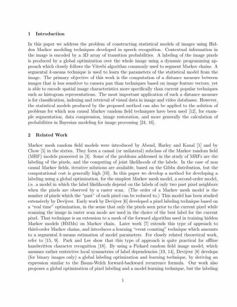
1 Introduction

In this paper we address the problem of constructing statistical models of images using Hid-den Markov modeling techniques developed in speech recognition. Contextual information inthe image is encoded by a 3D array of transition probabilities. A labeling of the image pixelsis produced by a global optimization over the whole image using a dynamic programming ap-proach which closely follows the Viterbi algorithm commonly used to segment Markov chains. Asegmental k-means technique is used to learn the parameters of the statistical model from theimage. The primary objective of this work is the computation of a distance measure betweenimages that is less sensitive to camera pan than techniques based on image feature vectors, yetis able to encode spatial image characteristics more specifically than current popular techniquessuch as histogram representations. The most important application of such a distance measureis for classification, indexing and retrieval of visual data in image and video databases. However,the statistical models produced by the proposed method can also be applied to the solution ofproblems for which non causal Markov random field techniques have been used [12], for exam-ple segmentation, data compression, image restoration, and more generally the calculation ofprobabilities in Bayesian modeling for image processing [24, 16].

2 Related Work

Markov mesh random field models were introduced by Abend, Harley and Kanal [1] and byChow [5] in the sixties. They form a causal (or unilateral) subclass of the Markov random field(MRF) models pioneered in [3]. Some of the problems addressed in the study of MRFs are thelabeling of the pixels, and the computing of joint likelihoods of the labels. In the case of noncausal Markov fields, iterative solutions are available, based on the Gibbs distribution, but thecomputational cost is generally high [10]. In this paper we develop a method for developing alabeling using a global optimization, for the simplest Markov mesh model, a second-order model,i.e. a model in which the label likelihoods depend on the labels of only two past pixel neighborswhen the pixels are observed by a raster scan. (The order of a Markov mesh model is thenumber of pixels which the “past” of each pixel can be reduced to.) This model has been studiedextensively by Devijver. Early work by Devijver [6] developed a pixel labeling technique based ona “real time” optimization, in the sense that only the pixels seen prior to the current pixel whilescanning the image in raster scan mode are used in the choice of the best label for the currentpixel. That technique is an extension to a mesh of the forward algorithm used in training hiddenMarkov models (HMMs) on Markov chain. Later work [7] extends this type of approach tothird-order Markov chains, and introduces a learning “event counting” technique which amountsto a segmental k-means estimation of model parameters. For closely related theoretical work,refer to [15, 9]. Park and Lee show that this type of approach is quite practical for offlinehandwritten character recognition [18]. By using a Pickard random field image model, whichassumes rather restrictive local symmetries of label dependencies [19, 14], Devijver [8] develops(for binary images only) a global labeling optimization and learning technique, by deriving anexpression similar to the Baum-Welch forward-backward recurrence formula. Our work alsoproposes a global optimization of pixel labeling and a model learning technique, but the labeling

1

optimization is similar to a Viterbi algorithm and the training is performed by a segmental-kmeans technique. Our approach does not require symmetry constraints on the Markov meshmodel, and it applies to color images.

A rather different tack for applying Hidden Markov models to images can be found in theliterature, the so-called “pseudo 2-D” HMM approach [13]. It does not attempt to model thelocal simultaneous dependencies of pixels to row and column neighbors. Instead, rows of theimage are segmented by a left-right version of 1-D HMM. Then the patterns of the segmentedrows can be grouped into vertical segments containing similar rows by applying an HMM in whichthe states (called superstates to avoid confusion with the states of the row HMMs) correspondto different families of segmentation patterns within rows. This technique is being applied inmany domains, for example in optical character recognition [13], color image retrieval [17], faceidentification [23]. The method proposed in this paper produces a more descriptive model ofimage statistics, in the sense that 2-D local mesh context is described by the model. Thereforeits domain of application potentially overlaps that of pseudo 2-D HMMs.

3 Notations

We consider a rectangular U × V image. For each pixel location (u, v), we have two quantities,an observable vector ou,v and a hidden state qu,v which can take the discrete values {1, 2, . . . , N}.The components of the observation vector ou,v for a pixel are the color components in this paper,but we could instead consider DCT coefficients, or the results of a local filter. The hidden statequ,v can be viewed as a label for the pixel. The total number of states N used in the modeling isspecified. The labeling of each pixel by a state provides a quantization of the observation vectors,and a segmentation of the image.

The relationship between observation vectors and states is part of the model and is expressedstatistically. The modeling process will compute the probability distributions of observationvalues given state values, P (o|q).

We also define:Ru,v the rectangle of image pixels defined by diagonal corner pixels (0, 0) and (u, v);xu,v the vector of combined state qu,v and observation ou,v at pixel (u, v): xu,v = (qu,v, ou,v);Qu,v and Ou,v the configurations of states and observations on rectangles Ru,v;Xu,v the rectangular configuration of joint states and observations on rectangles Ru,v.

We assume that the statistical properties don’t change across the image (in other words, therandom field is homogeneous). Therefore, often only relative pixel positions are important, andwe can simplify pixel index notations by omitting indices for the observed pixel, and using indexe for its east pixel, index n for its north pixel, and index ne for its north-east pixel.

Conditional probabilities for states at neighbor pixels are written P (q|qe, qn), which is short-hand for the full expression P (q = k|qe = i, qn = j), where i, j and k are the specific instances,or labels, taken by the pixel states. They define a 3D transition probability matrix.

Conditional probabilities for states at neighbor pixels will be written P (qu,v|qu,v−1, qu−1,v),which is shorthand for the full expression P (qu,v = k|qu,v−1 = i, qu−1,v = j), where i, j and k arethe specific instances, or labels, taken by the pixel states. We will assume the modeled field tobe homogeneous over the image; in other words, the probability just written will have the same

2

AAAAAAAAAAAAAAAAAAAAAAAAAAAAAAAAAAAAAAAAAAAAAAAAAAAAAAAAAAAAAAAAAAAAAAAAAAAAAAAAAAAAAAAAAAAAAAAAAAAAAAAAAAAAAAAAAAAAAAAAAAAAAA

AAAAAAAAAAAAAAAAAAAAAAAAAAAAAAAAAAAAAAAAAAAAAAAAAAAAAAAAAAAAAAAAAAAAAAAAAAAAAAAAAAAAAAAAAAAAAAAAAAAAAAAAAAAAAAAAAAAAAAAAAAAAAA

(u, v)

Ru-1,V

RU,v-1 (U,V)

(1, 1)

(u, v)

(U,V)

(1, 1)

AAAAAAAAAAAA

AAAAAAAAA

(u-1, v)

(u, v-1)

(a) (b)

Figure 1: With a second-order causal Markov mesh model applied to an image IU,V , the proba-bility of seeing a state i at (u, v) conditional to the state configurations for pixels in rectanglesRU,v−1, Ru−1,V (a) is equal to that probability conditional to the states of the left and topneighbors (b).

value for any pixel (u, v) wherever we consider the probability for the state of this pixel to bek, the state of the left pixel to be i and the state of the top pixel to be j. Therefore we willalso use aijk as shorthand for P (qu,v = k|qu,v−1 = i, qu−1,v = j) in discussions where geometricconsiderations are not important. The 3D matrix aijk is the transition matrix of the model, i.e.the probability while doing a raster scan of jumping to a pixel in state k if we just saw a pixelin state i in the same row and we had seen a pixel in state j in the same column in the previousrow.

4 Markov Mesh Properties

We assume the configuration of states in the image to be driven by a homogeneous second-orderMarkov random mesh model. The defining property is described in Fig. 1 and can be expressedas [1]:

P (qu,v|QU,v−1 ∪Qu−1,V ) = P (qu,v|qu,v−1, qu−1,v) (1)

where we relax the notations to mean the following at the boundaries:

P (qu,v|qu,v−1, qu−1,v) = P (q1,1) if u = v = 1

P (qu,v|qu,v−1, qu−1,v) = P (qu,1|qu−1,1) if u > v, v = 1

P (qu,v|qu,v−1, qu−1,v) = P (q1,v|q1,v−1) if v > u, u = 1

3

In other words, the probability of having a given state at pixel (u, v) conditional to the statesin all the pixels on the rows above row u and all the remaining pixels to the left of column v issimply equal to the probability of having that state at pixel (u, v) conditional to the state of thepixel above (u, v) and to the state of the pixel to the left of (u, v) (Fig. 1).Kanal and coworkers showed that the probability of seeing the configuration of states Qu,v overthe rectangle Ru,v is then equal to the product of the probabilities of each pixel in the rectangle,each probability being conditional to the states of the east and north neighbor pixels [1].

P (Qu,v) =u∏

u′=1

v∏

v′=1

P (qu′,v′ |qu′,v′−1, qu′−1,v′) (2)

This factorization is what makes this Markov model attractive. It is similar in form to thefactorization of the joint probability in a 1D Markov chain using first order dependencies betweenstates. However, the proof for this property is slightly more involved and is reproduced in theAppendix.

The observation ou,v at pixel (u, v) is assumed to depend only on the state qu,v at that pixel.Therefore a second factorization follows:

P (o1,1, o1,2, . . . , ou,v|q1,1, q1,2, . . . , qu,v) =u∏

u′=1

v∏

v′=1

P (ou′,v′|qu′,v′) (3)

or, using Ou,v and Qu,v to express the configuration of observations oi,j and qi,j over the rectangleRu,v,

P (Ou,v|Qu,v) =u∏

u′=1

v∏

v′=1

P (ou′,v′|qu′,v′) (4)

Now consider the event X defined by the joint occurrence of specific states q and observations oat pixels of rectangle R: By combining the factorizations of Eq. 2 and 4, it is straightforward toexpress X as the product of individual P (x) at each pixel of the rectangle:

P (Xu,v) = P (Ou,v, Qu,v)

= P (Ou,v|Qu,v)P (Qu,v)

= [u∏

u′=1

v∏

v′=1

P (ou′,v′ |qu′,v′)][u∏

u′=1

v∏

v′=1

P (qu′,v′|qu′−1,v′ , qu′,v′−1)]

=u∏

u′=1

v∏

v′=1

P (ou′,v′ |qu′,v′)P (qu′,v′ |qu′−1,v′ , qu′,v′−1)

=u∏

u′=1

v∏

v′=1

P (ou′,v′ |qu′,v′ , qu′−1,v′ , qu′,v′−1)P (qu′,v′ |qu′−1,v′ , qu′,v′−1)

=u∏

u′=1

v∏

v′=1

P (ou′,v′ , qu′,v′ |qu′−1,v′ , qu′,v′−1)

P (Xu,v) =u∏

u′=1

v∏

v′=1

P (xu′,v′ |qu′−1,v′ , qu′,v′−1) (5)

4

AAAAAAAAAAAAAAAAAAAAAAAAAAAAAAAAAAAAAAAAAAAAAAAAAAAAAAAAAAAAAAAAAAAAAAAAAAAAAAAAAAAAAAAAAAAAAAAAAAA

AAAAAAAAAAAAAAAAAAAAAAAAAAAAAAAAAAAAAAAAAAAAAAAAAAAAAAAAAAAAAAAAAAAAAAAAAAAAAAAAAAAAAAAAAAAAAAAA

AAAAAAAAAAAAAAAAAAAAAAAAAAAAAAAAAAAAAAAAAAAAAAAAAAAAAAAAAAAAAAA

(u, v)

Ru-1,v

Ru,v-1

Ru-1,v-1

(U,V)

(1, 1)

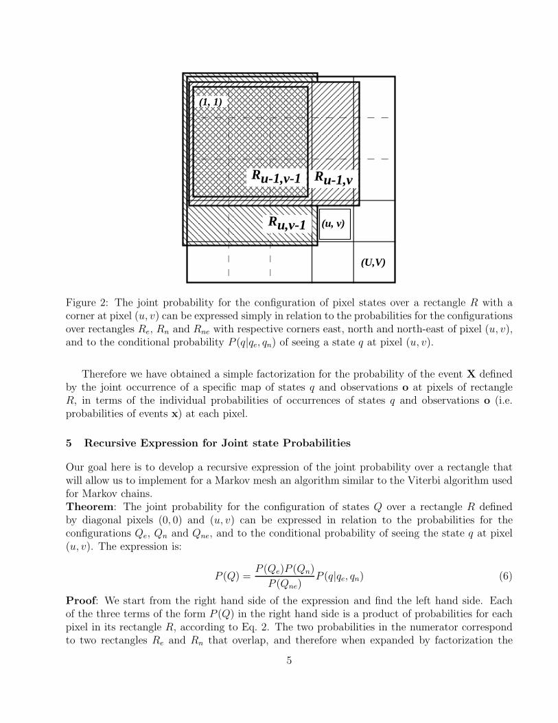
Figure 2: The joint probability for the configuration of pixel states over a rectangle R with acorner at pixel (u, v) can be expressed simply in relation to the probabilities for the configurationsover rectangles Re, Rn and Rne with respective corners east, north and north-east of pixel (u, v),and to the conditional probability P (q|qe, qn) of seeing a state q at pixel (u, v).

Therefore we have obtained a simple factorization for the probability of the event X definedby the joint occurrence of a specific map of states q and observations o at pixels of rectangleR, in terms of the individual probabilities of occurrences of states q and observations o (i.e.probabilities of events x) at each pixel.

5 Recursive Expression for Joint state Probabilities

Our goal here is to develop a recursive expression of the joint probability over a rectangle thatwill allow us to implement for a Markov mesh an algorithm similar to the Viterbi algorithm usedfor Markov chains.Theorem: The joint probability for the configuration of states Q over a rectangle R definedby diagonal pixels (0, 0) and (u, v) can be expressed in relation to the probabilities for theconfigurations Qe, Qn and Qne, and to the conditional probability of seeing the state q at pixel(u, v). The expression is:

P (Q) =P (Qe)P (Qn)

P (Qne)P (q|qe, qn) (6)

Proof: We start from the right hand side of the expression and find the left hand side. Eachof the three terms of the form P (Q) in the right hand side is a product of probabilities for eachpixel in its rectangle R, according to Eq. 2. The two probabilities in the numerator correspondto two rectangles Re and Rn that overlap, and therefore when expanded by factorization the

5

numerator has the probabilities for the pixels of the overlapping rectangle appearing twice asfactors (see Fig. 2). The probability of the denominator is for a rectangle Rne that is exactlyequal to the rectangle of overlap, therefore the factors appearing a second time in the numeratorare eliminated by simplification with the factors of the denominator. What is left is the productof all the probabilities that correspond either to rectangle Re or to rectangle Rn, but not both.This accounts for all the probabilities over rectangle R, except for the probability P (q|qe, qn)corresponding to pixel (u, v). Once this factor is included as shown in Eq. 6 we have all thefactors required to yield P (Q) according to Eq. 6.

Now, using Eq. 5, we can write the same type of decomposition for P (X) as for P (Q) andjustify it with the same proof:

P (X) =P (Xe)P (Xn)

P (Xne)P (x|qe, qn) (7)

6 Dynamic Programming Algorithm

In this section we will follow closely (for a second-order Markov model and a Markov mesh)the presentation made by Rabiner for the Viterbi algorithm applied to a first-order model ofa Markov chain [21, 22]. We are looking for the single best state configuration QU,V over thewhole image lattice for the given observation map (image) Ou,v, i.e. the state configuration thatmaximizes the probability P (Qu,v|Ou,v), or equivalently maximizes the probability P (Ou,v, Qu,v),which we called P (Xu,v). This is a global optimization problem, but thanks to the decompositionof Eq. 7, it can be solved by dynamic programming [2]. We define the quantity

δu,v(qu,v) = maxQu,v−{qu,v}

P (Qu,v,Ou,v) = maxQu,v−{qu,v}

P (Xu,v) (8)

where the notationQu,v−{qu,v} represents the configuration of states for all pixels of the rectangleRu,v, except pixel (u, v). Therefore, when maximized over Qu,v − {qu,v}, the expression remainsa function of qu,v.

Once we are able to compute such an expression for any (u, v), then the maximum jointprobability for the whole image configuration QU,V is simply:

maxQU,V

(P (QU,V ,OU,V ) = maxqU,V

δU,V (qU,V ) (9)

We apply the recursion expression of Eq. 7 in the definition 8 of δu,v(qu,v) and obtain arecursive equation for δu,v(qu,v) by the following steps:

δu,v(qu,v) = maxQu,v−{qu,v}

[P (Xu,v−1)P (Xu−1,v)

P (Xu−1,v−1)P (Xu,v|qu,v−1, qu−1,v)]

≃max{qu,v−1,qu−1,v}[δu,v−1(qu,v−1)δu−1,v(qu−1,v)P (xu,v|qu,v−1, qu−1,v)]

δu−1,v−1(q∗u−1,v−1)

δu,v(qu,v) = maxqu,v−1,qu−1,v

[δu,v−1(qu,v−1)δu−1,v(qu−1,v)P (qu,v|qu,v−1, qu−1,v)]P (ou,v|qu,v)

δu−1,v−1(q∗u−1,v−1)(10)

6

where 1 ≤ qu,v ≤ N and q∗u−1,v−1 is the state that corresponds to the best score for δu−1,v−1(k).We made use of properties such as

maxQu,v−{qu,v}

P (Xu,v−1) = maxqu,v−1

[ maxQu,v−1−{qu,v−1}

P (Xu,v−1)] = maxqu,v−1

δu,v−1(qu,v−1)

This expression is an approximation, in the sense that we have assumed that the maximum of theexpression is obtained when the common part P (Xu−1,v−1) between P (Xu,v−1) and P (Xu−1,v) ismaximum. This common part also appears at the denominator, and its maximum is δu−1,v−1(q

∗u−1,v−1).

The approximation assumes that the optimization of δ at (u, v) should not involve pixel (u −1, v − 1), which is in line with the second-order Markov mesh simplification assuming that thestates at these pixels are independent.

We don’t know the index q∗u−1,v−1 yet at the time we do the calculation. However the ar-guments qu,v−1 and qu−1,v that maximize Eq. 10 for each qu,v are independent of the value ofδu−1,v−1(q

∗u−1,v−1). Therefore, the main purpose of the Viterbi algorithm – finding the configura-

tion of optimal pixel states – can be achieved without attempting to compute the best possiblevalue for δu−1,v−1(q

∗u−1,v−1). The other purpose of the Viterbi algorithm – obtaining a correct

value for the joint probability – can be directly obtained once the optimum state configurationhas been computed, by applying Eq. 3.

The division by δu−1,v−1(q∗u−1,v−1) can be seen as a renormalization that prevents the prob-

abilities over the rectangle Ru−1,v−1 from being counted twice, since both δu,v−1(qu,v−1) andδu−1,v(qu−1,v) include these probabilities. Therefore, even if the term δu−1,v−1(q

∗u−1,v−1) is not di-

rectly instrumental in the computation of the optimal state configuration, we cannot simply setthis term to 1, because of this renormalizing effect. For larger images, the computation wouldbe subjected to underflow. However, any scaling technique is appropriate. One scaling tech-nique consists of computing this term for the state that maximizes it. Another scaling techniqueconsists of normalizing the components of each term δ as soon as it has been computed by Eq. 10.

As a third scaling technique, when the Viterbi algorithm is run in a iteration loop as describedin the training procedure below, the map of best states q∗u,v becomes available from previousscans and is refined in the iteration process. Then the Viterbi algorithm provides a correct jointprobability of states and observations at the end of the iteration, and applying Eq. 3 is notnecessary.

To retrieve the state map when the bottom right corner is reached, we need to keep track ofthe states qu,v−1 and qu−1,v that maximized Eq. 10. We store these values in the arrays ψH

u,v(qu,v)and ψV

u,v(qu,v) respectively, where the letters H and V are a reminder that these arrays are used tobacktrack along horizontal and vertical traces of the paths. The complete backtracking procedureis described in Step 4 below.

The steps of the Viterbi algorithm can be summarized as follows:

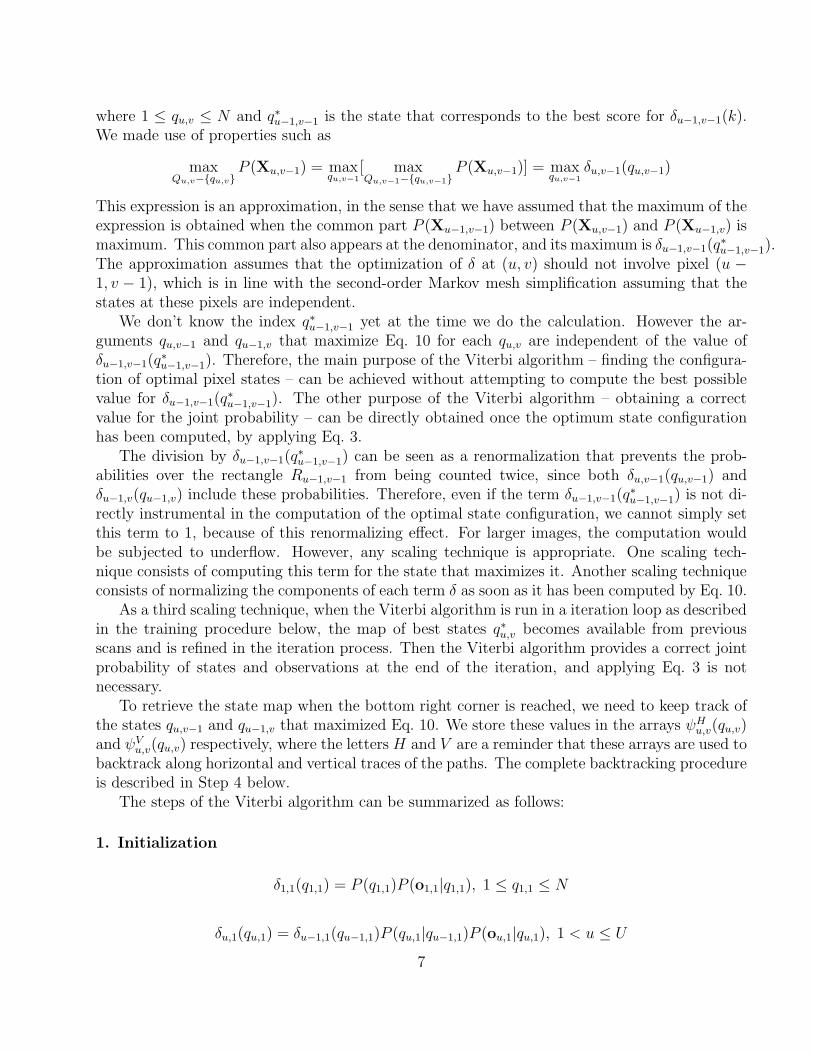
1. Initialization

δ1,1(q1,1) = P (q1,1)P (o1,1|q1,1), 1 ≤ q1,1 ≤ N

δu,1(qu,1) = δu−1,1(qu−1,1)P (qu,1|qu−1,1)P (ou,1|qu,1), 1 < u ≤ U

7

δ1,v(q1,v) = δ1,v−1(q1,v−1)P (q1,v|q1,v−1)P (o1,v|q1,v), 1 < v ≤ V

2. Recursion

δu,v(qu,v) = maxqu,v−1,qu−1,v

[δu,v−1(qu,v−1)δu−1,v(qu−1,v)P (qu,v|qu,v−1, qu−1,v)]P (ou,v|qu,v)

δu−1,v−1(q∗u−1,v−1)

(ψHu,v(qu,v), ψ

Vu,v(qu,v)) = arg max

qu,v−1,qu−1,v

δu,v(qu,v)

3. Termination

P ∗(QU,V ,OU,V ) ≡ maxQU,V

(P (QU,V ,OU,V ) = maxqU,V

δU,V (qU,V )

q∗U,V = arg maxqU,V

δU,V (qU,V )

4. Path (state map) backtracking

The optimal states for image pixels can be obtained by backtracking from the known best stateof the bottom right pixel (U, V ). However, there are multiple ways of arriving at any pixel, andeach may result in a different selected state.

For example, consider an image in which each pixel can be labeled by state 1, 2 or 3 (Fig. 3).These 3 states are represented by a vertical pile of 3 boxes at each pixel, and in each state box wewrote the number of paths starting from pixel (U, V ) that have reached that state when passingthrough the pixel. When backtracking from pixel (U, V ) to pixel (U − 1, V − 2) there are threepaths.

1. Path H −H − V :

q∗U,V = 2, ψHU,V (2) = 3, ψH

U,V −1(3) = 3, ψVU,V −2(3) = 2

2. Path V −H −H :

q∗U,V = 2, ψVU,V (2) = 3, ψH

U−1,V (3) = 3, ψHU−1,V −1(3) = 1

3. Path H − V −H :

q∗U,V = 2, ψHU,V (2) = 3, ψV

U,V −1(3) = 3, ψHU−1,V −1(3) = 1

8

(U,V)

(1, 1)

01

0

00

1

00

2

21

0

00

1

00

1

3

3

3

3

3

1

2

Figure 3: The best states q∗u,v for each pixel (u, v) are those that are reached by the highestnumber of backtraces from the best state of the lower right corner of the image, using backtrackingmatrices ψH

u,v−1 and ψVu−1,v.

Thus for pixel (U − 2, V − 1) we arrive at state 2 if we backtrack horizontally twice, thenvertically; state 1 if we backtrack vertically, then horizontally twice; and state 1 again if webacktrack horizontally, vertically, then horizontally again.

There are ways of enforcing the consistency of alternate paths within each recursion stepwithin the dynamic programming process, however this local decision process could reduce thequality of the optimization.

Instead, we take the approach of selecting as best state for a pixel the state which is obtainedby the largest number of backtracking paths. For the example above, state 1 would be selectedfor pixel (U − 1, V − 2) because it is reached twice, whereas state 2 is reached only once, andstate 3 is not reached at all.

Therefore for each pixel (u, v), we keep the count of the number of times each state hasbeen reached by a backtracking path. This does not require enumerating the paths, and can beperformed for the whole image in time proportional to the number of pixels, by noticing thatall the paths to pixel (u, v) have to come from either (u, v + 1) or from (u + 1, v), so that thepath counts for (u, v) are obtained locally by transmitting the path counts at (u, v + 1) and at(u+ 1, v), along the subpaths defined by ψH

u,v and ψVu,v.

For each pixel the path counts for each state i are kept as components i of a vector Su,v(i).The process starts with the pixel at the lower right corner of the image with a path count of1 for state q∗U,V (found at the termination step described above) and zero for the other states.Therefore the algorithm is as follows:

9

(a) (b) (c)

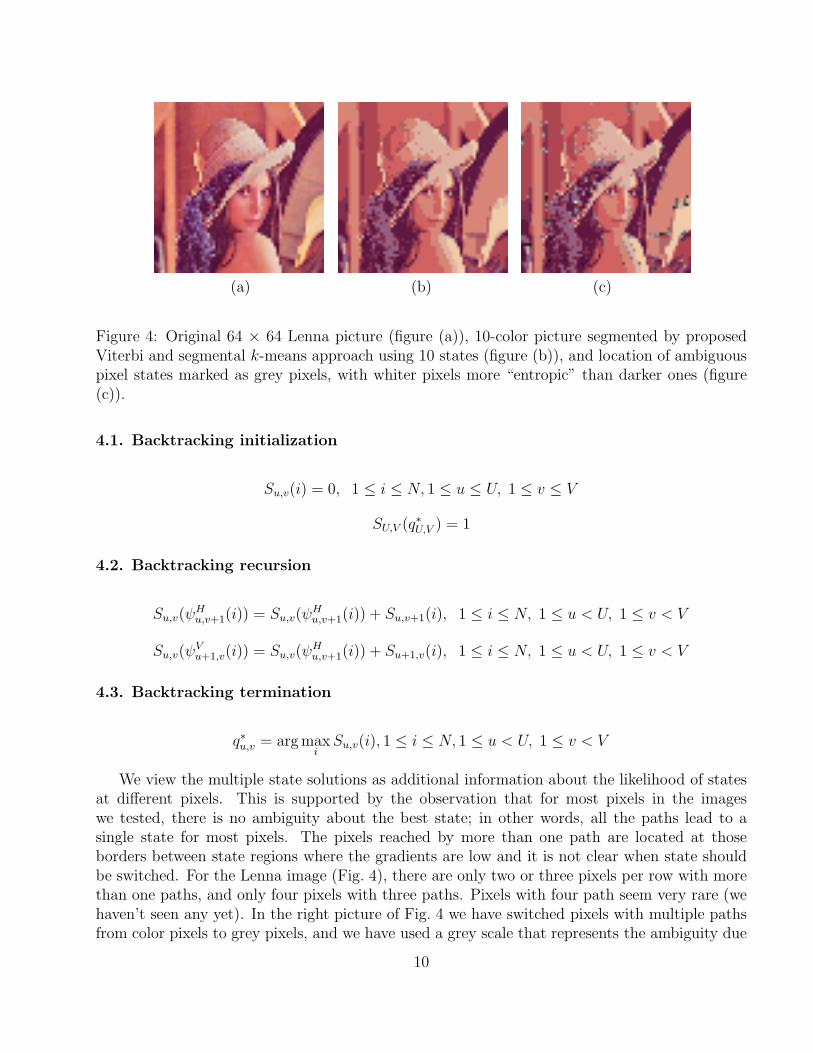
Figure 4: Original 64 × 64 Lenna picture (figure (a)), 10-color picture segmented by proposedViterbi and segmental k-means approach using 10 states (figure (b)), and location of ambiguouspixel states marked as grey pixels, with whiter pixels more “entropic” than darker ones (figure(c)).

4.1. Backtracking initialization

Su,v(i) = 0, 1 ≤ i ≤ N, 1 ≤ u ≤ U, 1 ≤ v ≤ V

SU,V (q∗U,V ) = 1

4.2. Backtracking recursion

Su,v(ψHu,v+1(i)) = Su,v(ψ

Hu,v+1(i)) + Su,v+1(i), 1 ≤ i ≤ N, 1 ≤ u < U, 1 ≤ v < V

Su,v(ψVu+1,v(i)) = Su,v(ψ

Hu,v+1(i)) + Su+1,v(i), 1 ≤ i ≤ N, 1 ≤ u < U, 1 ≤ v < V

4.3. Backtracking termination

q∗u,v = arg maxiSu,v(i), 1 ≤ i ≤ N, 1 ≤ u < U, 1 ≤ v < V

We view the multiple state solutions as additional information about the likelihood of statesat different pixels. This is supported by the observation that for most pixels in the imageswe tested, there is no ambiguity about the best state; in other words, all the paths lead to asingle state for most pixels. The pixels reached by more than one path are located at thoseborders between state regions where the gradients are low and it is not clear when state shouldbe switched. For the Lenna image (Fig. 4), there are only two or three pixels per row with morethan one paths, and only four pixels with three paths. Pixels with four path seem very rare (wehaven’t seen any yet). In the right picture of Fig. 4 we have switched pixels with multiple pathsfrom color pixels to grey pixels, and we have used a grey scale that represents the ambiguity due

10

to multiple paths, using an entropy measure. The ambiguity is zero if there is only one path, andit is close to zero if there are two paths but the path count for one is a much larger proportionof the total path count for the pixel than the other path count. It is maximum if there are alarger number of paths with almost equal path counts. Entropy is a good measure of this typeof ambiguity. It is computed as −

∑Ni=1 ciLog(ci) where ci is the path count for state i. The grey

levels are normalized so that the pixel with the maximum entropy is white, and the pixel withminimum non zero entropy is black (pixels with zero entropy retain their original color).

7 Modeling of observation probabilities

As mentioned above, as is customary for HMMs in speech recognition, the distributions of ob-servations are assumed to depend on the states of the pixels only, and not on the observations ofneighbor pixels (the relationship between pixels is modeled by the statistics of the pixel states).Therefore what we model is the mean and the variability of the observations at the pixels thathave been labeled by the same states. For example, if we take as observation vectors the 3 colorcomponents of the pixels, state labeling tends to segment the image into large regions of similarcolor, and the modeling of the color components models the variations of colors within each typeof region. If the components of the observation vector are selected to be approximately inde-pendent, the distribution of each component can be independently modeled with a histogram(non-parametric discrete modeling of observations), with a normal distribution, or with a mixtureof gaussians (continuous observation densities).

For color images, we have used normal distributions to model each of the three color com-ponents, and taken the observation probability of a pixel as the product of the probabilities ofobservations of the color components. This assumes that the color components are independent.Even as (R,G,B) components are more interdependent than components in color spaces thatuse luminance, hue and saturation, we have not observed qualitative improvements in segmenta-tion when using the (Y, U, V ) components of JPEG and MPEG compression instead of (R,G,B)components.

8 Training

We now address the problem of learning the model of a given image. In order to apply theViterbi algorithm presented in Section 6, the quantities P (qu,v|qu,v−1, qu−1,v) and P (ou,v|qu,v)must be known before a meaningful state assignment for each pixel can be obtained. The firstquantities represent the transition matrix of the model: given that the left pixel is in statequ,v−1 and the top pixel in state qu−1,v what is the probability for the present pixel to be instate qu,v from 1 to N . The second quantities are the observation probabilities, that we assumein this presentation to be modeled by the product of the probabilities of the component of theobservations, each modeled by a normal distribution. Assuming we can run the Viterbi algorithmto obtain a state assignment, then these probabilities can be easily computed, by scanning theimage, and (1) tallying and normalizing the different types of state transitions between pixelsto obtain the state transition matrix, and (2) averaging the values of observation componentsand their squares for all pixels with the same state labels to estimate the mean and variance of

11

observation components for pixels of identical states. This is a chicken-and-egg problem in thesense that we need these distributions to compute the Viterbi algorithm, and we need the Viterbialgorithm to compute the distributions.

This problem is solved by putting the Viterbi algorithm in an iteration loop. The iterationstarts with random transition probabilities in the state transition matrix, while the gaussians ofthe observation component probabilities can be initially selected to overlap and cover the rangeof possible observations. As Viterbi segmentations and probability estimations are repeated al-ternately, the joint probability of the configuration of observations and states increases (althoughthe general increase is not guaranteed to be locally monotonic as with a Baum-Welch procedure)as the system consistently converges to a stable solution. The exit criterion that we use is themaximum variation of the parameters of the model from step to step. Typically, little qualitativeimprovement can be observed in the image segmentation after 10 iterations. The results are astatistical model of the image, a segmentation of the image, and an evaluation of the proba-bility of observing the image given the model. This technique is called a segmental k-meansprocedure [21]. It is popular in speech recognition as a much faster model training alternativeto the Baum-Welch procedure, with comparable quality of results. In our case, we do not havean extension of the so-called forward-backward procedure for Markov meshes, so we cannot usea Baum-Welch approach.

9 Color segmentation with this model

One of the results of the training procedure described above is an optimal labeling of the image.Once a labeling is obtained, one may want to show the segmented image with the most likely colorfor each labeled pixel. For each state label, the most likely color is the color whose components arethe most likely, because we have assumed that the components are independent. The distributionof each component within each state is modeled by a normal distribution. The most likely colorcomponent in each state is the mean of its normal distribution in this state. The most likelycolor is then obtained by combining these components. Fig. 4 shows a 64 × Lenna image (a),and a segmentation obtained using 10 states (b). Note that the number of states is the onlyspecified parameter of this segmentation.

9.1 Distances between Images

In videos, successive frames of the same scene are typically views of the same objects whoseimages are shifted in the frames due to the camera’s panning action, and we would like to assessthat despite very different local frame pixel values after large camera pans, such frames are stillsimilar. Statistical models of images characterize images, and allow computations of distances,yet are relatively insensitive to translation.

A distance measure can be computed as follows. We construct a probabilistic model λ1 ofone image I1, and to find the distance to a new image I2 we ask: what is the probability that N2

observations O on the new image I2 could have been produced by the probabilistic model λ1 ofthe first image? Such a probability is generally quite small and of the form P (I2|λ1 = 10−D, withD larger for more different images. Therefore D, which is the negative log of the probability,

12

− logP (I2|λ1), is an intuitive distance measure. To factor out the dependency of the totalprobability of the observation sequence on the number of observation, we normalize this measureby dividing by the number of observations N2. In addition, this measure applied between animage and itself is not zero with this definition, so in most applications a measure shifted by theimage distance to itself is preferable. Hence we obtain

D(I1, I2) =1

N2

logP (I2|λ1) −1

N1

logP (I1|λ1) (11)

This distance measure requires the calculation of the model λ1 of the first image only, but itis not symmetrical. When time to compute a model for the second image is available, one willprefer to compute a symmetrical distance measure Ds as the half sum of D(I1, I2) and D(I2, I1)

Ds(I1, I2) =1

2[logP (I2|λ1) − logP (I2|λ2)

N2

+logP (I1|λ2) − logP (I1|λ1)

N1

] (12)

Other interpretations of this expression exist in terms of model dissimilarity and cross-entropyof models ([21], p. 365)

9.2 Experiments with Distances

An example of distance calculation is shown in Fig. 5. We used the Lenna and Mandrill imagesto generate a composite third image in which a piece of the Lenna image image is replaced by apiece of the Mandrill image. We obtain an “image triangle” and compute the distances betweenits vertices using Eq. 12.

We compute distances between the images by obtaining a Markov model λi for each of theimages, then by computing the probabilities of observing all the pixels of image Ij assumingthat they were produced by model λi. The parts of the composite image that contain parts ofLenna’s image are well predicted by Lenna’s model, so they contribute to producing a largerjoint probability and a smaller distance between Lenna and the composite image. We find adistance of 1.2. Similarly, the distance between the Mandrill image and the composite image issmall, 2.0. On the other hand the Lenna and Mandrill image don’t have much in common, andwe find a distance of 5.9. Note that the triangle inequality is not satisfied in this example, andtherefore our distance measure is not a metric. People try to find distance measures that aremetrics because it allows for more efficient search, by the following reasoning: if I have an itemA and am looking for similar ones in a database, if I find an item B that is not similar at all toA, then I don’t need to check any of the items that are similar to B, because those other items,being close to B, will be unrelated to A. This reasoning is not necessarily desirable for imagedatabases. If I look for images of cows, I would not want to miss the images of a cow that alsocontains the farmer, just because in the database there is a picture of the farmer and a pictureof a cow, and the farmer does not look like his cow. And searches for Lenna should not failas soon a monkey walks into the room. Therefore there is an incompatibility between the needfor efficient search and the need for searches that are sensitive to partial matches and semanticcontent.

Another verification of the merit of this method can be obtained by taking an image, andscrambling it by swapping two pieces of the image. Example of images after 1, 5 and 10 scram-

13

5.9

2.01.2

Figure 5: Distance measures between HMM models for 2 images and a composite image.

(a) (b) (c)

Figure 6: Increasingly scrambled images obtained by randomly swapping 1, 5 and 10 squareregions.

14

0

0.5

1

1.5

2

2.5

3

3.5

0 2 4 6 8 10

"distSymLennaNoDur.txt"

Figure 7: Distances between Lenna picture and increasingly scrambled pictures obtained byswappings of square regions. Abscissas show number of swapping, and ordinates show distancesto original image. Distances are averages over 10 trials, and error bars are ± standard deviations.Some random swappings may reverse the scrambling of a previous swapping.

15

blings are shown in Fig. 6. As scrambling increases, the distance from the original image to thescrambled image increases as the image gets more scrambled, as shown in the plot of Fig. 7. Thisis an intuitive result, which would be difficult to obtain with distance measures which rely onfeature matchings.

10 Semi-Markov Model with Explicit State Dimension Probabilities

In speech recognition, the probability of staying in the same state obtained by standard Markovmodeling often lacks flexibility, and explicitly modeling ”state durations” in analytic form wasshown to improve performance [21]. The model then does not follow a Markov model as longas the model stays in the same state, and is called a semi-Markov model. For a Markov meshmodeling applied to images, similar limitations of the standard model can be observed whentrying to model the width and height of regions of contiguous pixels of identical states with aMarkov mesh model.

With a state transition matrix P (qu,v|qu,v−1, qu−1,v), or, borrowing the simpler notation ofRabiner [21], aijk (where k is the value taken by the state qu,v of pixel (u, v), and i and j arethe states at left and top pixels respectively), the probability of staying in the same state khorizontally along a row is

Pk(dH) = (N∑

j=1

akjk)dH−1(1 −

N∑

j=1

akjk)

and the probability for pixels of same state i to be connected vertically is

Pi(dV ) = (N∑

i=1

aikk)dV −1(1 −

N∑

i=1

aikk)

This type of distribution is exponential. It is monotonically decreasing with increasing regionsize, either horizontally or vertically. Therefore small blobs are modeled as being more probablethan larger blobs. Instead, for a model that is trained on an image with redish regions thatare mostly 10 pixel wide and 20 pixel high, we would like the model of probability distributionof ”state dimensions” to have a maximum at around 10 pixels for the horizontal dimension ofcontiguous red pixels, and around 20 pixels for the vertical dimension.

For modeling durations, the Gamma distribution was found to produce a good fit to observedduration histograms [4]. It assigns zero probabilities to negative values of the variable, which isvery desirable for modeling durations or dimensions. This distribution is of the form

p(x) =αp

Γ(p)e−αxxp−1 (13)

The two free parameters of the distribution are α and p. For this application, they arepositive, as seen from their estimation expressions below. The parameter α controls the verticalscaling of the distribution, while p controls whether there is a peak or not and where the peak islocated. For p < 1, a monotonically decreasing distribution is modeled, otherwise a peak occursat p−1

α. The curve shape is less skewed and more gaussian-like as the peak is located further

16

from the origin. The two parameters of the Gamma distribution can be simply estimated fromthe mean x and variance x2 of the data x by

α =x

x2, p =

x2

x2

Burshtein proposed heuristic expressions for forcing the state durations to approximately fol-low a Gamma distribution in a speech recognition system [4]. However, obtaining an exact matchis straightforward enough, therefore this is the technique preferred here. The cumulative prob-ability corresponding to the Gamma distribution is called an incomplete Gamma function [20].Its complement to 1, Pk(d), represents, for a state k, the probability that the region dimensionD will be more than a given dimension d. If we were in a state qu,v−1 = k at the previous pixelof the same row and have been in this state for a distance of d− 1 pixels, the probability of stillbeing in the state k at pixel (u, v) is the probability that the region’s horizontal dimension D

will be larger than d, given the fact that it is already larger than d− 1. Therefore

Pstay(k, d) =Pk(d)

Pk(d− 1)(14)

The only other possibility is that we leave state k when we go to the next pixel, therefore theexpression for the probability of leaving state k is the complement to 1 of the previous probability.

We can apply this technique to model region shapes in many ways. In our current imple-mentation, we model both the horizontal distance (in pixels) from the top left pixel of a stateregion to its right edges, and the vertical distance from the top left pixel to its bottom edges.To train this model within the segmental k-means framework described above, as we scan animage that has been segmented into state regions by the Viterbi algorithm described above, wecompute horizontal and vertical distances for each pixel using distance information passed fromneighbors. If the current pixel of state k is connected to a top or right neighbor of the samestate, the information about the location of the top left pixel for that region is updated fromthese neighbors to the current pixel, and the vertical and horizontal distances from that top leftpixel are also updated. The top left pixel of a new region of state k is a pixel of state k that isnot connected to a top pixel of state k or a left pixel of state k. If the current pixel of state khas a left neighbor of state i different from k, then we went off a right edge for a state region i.We read the horizontal distance for that neighbor and use it to build up the sums used to obtainits mean and variance in regions of state i. From such means and variances, we can computegamma distributions for these quantities, and compute the probability of staying in a state orleaving it as described above.

We define the following notations:

• SHi probability of staying in state i horizontally, i.e. probability that the state of current

pixel be the same as state i of its left neighbor.

• LHi probability of leaving state i horizontally, i.e. probability that current pixel be in a

state k different from state i: LHi = 1 − SH

i

• SVj probability of staying in state j vertically, i.e. probability that the state of current pixel

be the same as state j of its top neighbor.

17

• LVj probability of leaving state j vertically, i.e. probability that current pixel be in a state

k different from state j: LVj = 1 − SH

j

Each of these probabilities depends on state dimensions dH or dV , and is computed by Eq. 14or its complement to 1. We construct tables for each state to provide these probabilities forhorizontal and vertical state dimensions from 1 to the width and heigth of the image.

Assume that we have obtained by segmental k-means training the transition matrix aijk thattabulates the probability of having the current pixel (u, v) of being in state k when the leftpixel (u, v − 1) is in state j and the top pixel (u − 1, v) is in state j. We wish to compute anew transition matrix a′ijk that accounts for the modeling of dimensions of state regions. If kis equal to i or j (or both if i and j are equal) then the current pixel is still in the same stateand we ignore the inadequate exponential distribution that the transition matrix would providefor the probability or staying in the same state, replacing it by a combination of probabilities ofseeing the observed region dimensions in the horizontal and vertical directions. If however thestate k of the current pixel is different from both i and j, then the information provided by thetransition matrix is adequate, but must be combined with the probabilities of leaving the regionsof the neighbor pixels in a consistent way so that the probabilities in the third dimension of theresulting matrix aijk add up to 1 (since for given top and left pixel states, the current pixel mustbe in one of the state k = 1, . . . , N .) Such a combination is provided here:

1. i = j

(a) k = i (⇒ k = j)

a′iii =SH

i SVi

SHi S

Vi + LH

i LVi

(b) k 6= i (⇒ k 6= j)

a′iik =LH

i LVi

SHi S

Vi + LH

i LVi

aiik

(1 − aiii)

2. i 6= j

(a) k = i (⇒ k 6= j)

a′iji =SH

i LVj

SHi L

Vj + SH

i LVj + LH

i LVj

(b) k 6= i, k = j)

a′ijj =LH

i SVj

SHi L

Vj + SH

i LVj + LH

i LVj

(c) k 6= i, k 6= j)

a′ijk =LH

i LVj

SHi L

Vj + SH

i LVj + LH

i LVj

aijk

(1 − aiij − aijj)

18

10.1 Comparison of Field Realizations

The improvement of image modeling provided by the explicit modeling of region dimensions canbe verified by comparing realizations of Markov fields obtained by the plain Markov model andby the semi Markov model.

We obtain these realizations by generating random colors from top left to bottom right alonga raster scan. States are produced to follow the transition probabilities a′ijk of the model trainedon images, with decisions to leave regions produced by Gamma deviates. States are mapped tocolors whose components are the means of the normal distributions that model the observations.In Fig. 8, we show realizations for models trained with three images, an image with ellipsesof different colors and aspect ratios, the Lenna image, and the Mandrill image (left column).The fields of the middle column are obtained with the plain Markov model, and the fields ofthe right column are obtained with the semi-Markov model approach. Note that the regionsizes, aspect ratios and contiguities are much closer to those of the regions of the original imageswith the semi-Markov model. A drawback of causal modeling in general is that context can beonly verified from previously generated pixels in the raster scan, so there are strong diagonaldirectional effects for large regions. For a comparison of realizations of MRF models and causalMarkov mesh models for mostly binary images, refer to [11].

Although large regions seem to be better modeled by the semi Markov model than by thestandard model, we do not notice a clear advantage of the improved model in image classificationusing the image distances described above. For example, the diagram of distances for increasinglyscrambled images of Fig. 6 is almost identical for the two models. One would have expected thesemi Markov model to respond to the chopping of the larger regions by the scrambling process byproducing larger distance increases than the standard model. More investigations are required.

11 Implementation Issues

Computation time for the Viterbi algorithm is proportional to O(U × V × (N3 +N ×D), whereU and V are the height and width of the image, N is the specified number of states, and D isthe number of components of the observation vectors at each pixels (3 for color images, 64 forDCT coefficients). The first term in the parenthesis of the computation cost is due to the tripleloop of the algorithm in which for each pixel, each of the N components of δ (Eq. 10) must findthe maximum of a term that includes one of the N components of the δ of the left pixel and oneof the N components of the δ of the top pixel. The second term is due to the computation ofthe observation probabilities of each pixel for each possible state, P (ou,v|qu,v). This second termmay become of the same order as the first term if we consider large observation vectors (andsmaller images), as when using DCT coefficients as observation vector components in order tofind Markov models of JPEG images.

All the computations in the Viterbi algorithm are performed using the logarithmic forms ofthe proposed expressions. The logarithms of the N3 elements of the transition matrix aijk andof the U × V × N probabilities P (ou,v|qu,v) at each Viterbi iteration in the segmental k-meansalgorithm are precomputed.

Each Viterbi iteration takes around 4 seconds for a 64×64 24 bit color image on an Ultra 1 Sunworkstation, and a full HMM and an image segmentation are obtained in around 40 seconds.

19

(a) (b) (c)

(d) (e) (f)

(g) (h) (i)

Figure 8: Realizations of Markov mesh models trained on images of the left column. Middlecolumn: Standard HMM. Right column: HMM with state dimension modeling.

20

The processing of 512 × 512 24 bit color images would be prohibitive in time (more than 40minutes) and memory requirements (large precomputed tables). The processing of JPEG imageswithout decompression is more attractive and is being investigated.

Computation time is significantly longer (presently by a factor of 4) when the semi Markovmodel is used. The reason is that the expressions for the N3 elements a′ijk are not precomputedbecause they depend not only on states i, j, and k, but also on the dimensions of regions, whichcan be as large as the image. Required tables would be very large (U × V ×N3).

Once Markov models of individual images are obtained, the computational cost for obtainingdistance measures between images is small, O(U × V ×D).

12 Conclusions and Comments

The main contribution of this paper is the decription of a training method for acquiring statisticalmodels of images using a hidden second order Markov mesh model. This model encodes the con-tiguities of image regions of similar properties, and the distributions of the pixel attributes withineach region. The method also provides an optimal segmentation of images when the number oflabels to be used is specified. Distances between images can be computed as distances betweenstatistical models of these images. We showed using composite images that these distances arevery sensitive to common image content without the need for feature matching. We are currentlyextending the model to use different states for different regions, as a 2D extension of the so calledleft-right HMMs, in order to provide improved object recognition capability. Applications beinginvestigated are classification in image data bases, image restoration in MPEG video streams,robust cut and transition detection in videos, change detection in streams from static cameras,and object recognition. The range of potential applications include the domains in which MRFmodels and pseudo 2-D HMMs have been applied, for example segmentation, data compressionand image restoration for MRFs, and character recognition and face recognition for pseudo 2-DHMMs.

Appendix

The defining property for the second-order Markov mesh is

P (qu,v|{QU,v−1 ∪Qu−1,V }) = P (qu,v|qu,v−1, qu−1,v) (15)

with the following boundary conditions

P (qu,v|qu,v−1, qu−1,v) = P (q1,1) if u = v = 1

= P (qu,1|qu−1,1) if u > v, v = 1

= P (q1,v|q1,v−1) if v > u, u = 1

In other words, the probability of having a given state at pixel (u, v) conditional to the statesin all the pixels on the rows above row u and all the remaining pixels to the left of column v is

21

simply equal to the probability of having that state at pixel (u, v) conditional to the state of thepixel above (u, v) and to the state of the pixel to the left of (u, v).

Note that this definition 15 can be applied to any subimage of the image IU,V , provided thatthe subimage contains pixel (u, v). For example, we can write

P (qu,v|Qu,v − {qu,v}) = P (qu,v|qu,v−1, qu−1,v) (16)

To see this, we simply apply the definition 15 to the subimage that extends from (1, 1) to(u, v). In this subimage, the configuration {QU,v−1 ∪ Qu−1,V } is identical to the configurationQu,v − {qu,v}.

We want to prove that the probability of seeing the configuration of states Qu,v over therectangle Ru,v is equal to the product of the probabilities of each pixel in the rectangle, eachprobability being conditional to the states of the top and left neighbor pixels.

P (Qu,v) =u∏

u′=1

v∏

v′=1

P (qu′,v′ |qu′−1,v′ , qu′,v′−1)

For u = 2, v = 1, the definition of a Markov mesh along with the boundary conditions yields

P (Q2,1) ≡ P (q1,1, q2,1) = P (q2,1|q1,1)

and for the first row and first column of pixels, the theorem amounts to the factorization of a1D Markov chain. We assume that the theorem holds for Qu,1 and show that it holds for Qu+1,1.

P (Qu+1,1) ≡ P (q1,1, q2,1, , q3,1, . . . , qu,1, qu+1,1)

P (Qu+1,1) = P (qu+1,1|Qu,1)P (Qu,1)

= P (qu+1,1|qu,1)P (Qu,1)

= P (qu+1,1|qu,1)P (qu,1|qu−1,1) . . .

. . . P (qu−1,1|qu−2,1) . . . P (q1,1)

Following [1], we assume that the theorem holds for Qu,v, and show that it holds for Qu+1,v.Induction for Qu+1,v is shown in the same way because of the symmetry of the expressions.

P (Qu+1,v) = P (Qu,v)P (qu+1,v, qu+1,v−1, . . . , qu+1,1|Qu,v)

= P (Qu,v)P (qu+1,v|qu+1,v−1, . . . , qu+1,1, Qu,v) . . .

. . . P (qu+1,v−1|qu+1,v−2, . . . , qu+1,1, Qu,v) . . .

. . . P (qu+1,1|Qu,v)

Using the Markov mesh defining property for each term of the factorization yields

22

P (Qu+1,v) = P (Qu,v)P (qu+1,v|qu+1,v−1, qu,v) . . .

. . . P (qu+1,v−1|qu+1,v−2, qu,v−1) . . .

. . . P (qu+1,1|qu+1,1, qu,1)

= P (Qu,v)v′=v∏

v′=2

P (qu+1,v′ |qu+1,v′−1, qu,v′)

=u′=u+1∏

u′=1

v′=v∏

v′=1

P (qu′+1,v′ |qu′+1,v′−1, qu′,v′)

Acknowledgements

The support of this research by the Department of Defense under contract MDA 9049-6C-1250is gratefully acknowledged.

References

[1] Abend, K., Harley, T.J, and Kanal, L.N., “Classification of Binary Random Patterns”, IEEETrans. Information Theory, IT-11, pp. 538–544, 1965.

[2] Ballard, D.H., and Brown, C.M., Computer Vision, Prentice-Hall, Englewood Cliffs, NJ,1982, pp. 137–143.

[3] Besag, J., “Spatial Interaction and the Statistical Analysis of Lattice Systems (with Discus-sion)”, J. Royal Statistical Society, series B, vol. 34, pp. 75–83, 1972.

[4] Burshtein, D., “Robust Parametric Modeling of Durations in Hidden Markov Models”,IEEE, 1995.

[5] Chow, C.K., ”A Recognition Method using Neighbor Dependence”, IRE Trans. on ElectronicComputers, vol. 11, pp. 683–690, 1962.

[6] Devijver, P.A., “Probabilistic Labeling in a Hidden Second Order Markov Mesh”, PatternRecognition in Practice, II, E.S. Gelsema and L.N. Kanal eds., North-Holland, Amsterdam,1986.

[7] Devijver, P.A., “Real-Time Modeling of Image Sequences”, Proc. 10th International Con-ference on Pattern Recognition, 1990, pp. 194-199.

[8] Devijver, P.A., and Dekesel, M.M., “Learning the Parameters of a Hidden Markov RandomField Model: A Simple Example”, Pattern Recognition Theory and Practice, P.A. Devijverand J. Kittler, eds, 1987.

[9] Fassnacht, C., and Devijver, P.A., “Image Segmentation with a Propagator Markov MeshModel”, Proc. 12th International Conference on Pattern Recognition, Jerusalem, 1994.

23

[10] Geman, S., and Geman, D., “Stochastic Relaxation, Gibbs Distribution, and the BayesianRestoration of Images”, IEEE Trans. Pattern Analysis and Machine Intelligence, vol. PAMI-6, no. 6, pp. 721–741, 1984.

[11] Gray, A.J., Kay, J.W., and Titterington, D.M., “An Empirical Study of the Simulation ofVarious Models Used for Images”, IEEE Trans. Pattern Analysis and Machine Intelligence,vol. PAMI-16, no. 5, pp. 507–513, 1994.

[12] Kashyap, R.L., and Chellappa, R., “Estimation and Choice of Neighbors in Spatial Interac-tion Models of Images”, IEEE Trans. Information Theory, vol. TI-29, pp. 60–72, 1983.

[13] Kuo, S-S. and Agazzi, O.E., “Keyword Spotting in Poorly Printed Documents using Pseudo2-D Hidden Markov Models”, IEEE Trans. Pattern Analysis and Machine Intelligence, vol.16, no, 8, pp. 842–848, 1994.

[14] Haslett, J., “Maximum Likelihood Discriminant Analysis on the Plane using a MarkovianModel of Spatial Context”, Pattern Recognition, 18, pp. 287–296, 1985.

[15] Lacroix, V., “Pixel Labeling in a Second-Order Markov Mesh”, Signal Processing 12, pp.59–82, 1987.

[16] Li, S.Z., Markov Random Field Modeling in Computer Vision, Springer, 1995.

[17] Lin, H-C., Wang, L-L., and Yang, S-N., “Color Image Retrieval Based on Hidden MarkovModels”, IEEE Trans. Image Processing, vol. 6, no. 2, pp. 332–339, 1984.

[18] Park, H.-S., and Lee, S.-W., “ An HMMRK-Based Statistical Approach for Off-line Hand-written Character Recognition”, Proceedings of ICPR, pp. 320–324, 1996.

[19] Pickard, D.K., ‘Unilateral Markov Fields”, Advanced Applied Probability, 12, pp. 655–671,1980.

[20] Press, W.H., Teukolsky, S.A., Vettering, W.T., and Flannery, B.P., Numerical Recipes in C,Second Edition, Cambridge University Press, 1992.

[21] Rabiner, L.R., and Juang, B.-H., “Fundamentals of Speech Processing”, Prentice Hall, pp.321–389, 1993.

[22] Rabiner, L.R., “A Tutorial on Hidden Markov Models and Selected Applications in SpeechRecognition”, Proceedings of the IEEE, vol. 77, no. 2, pp. 257–286, 1989.

[23] Samaria, F., and Young, S., “HMM-based architecture for Face Identification”, Image andVision Computing, vol. 12, no. 8, 1994.

[24] Szeliski, R., “Baysian Modeling of Uncertainty in Low-Level Vision”, Kluwer AcademicPublishers, 1989.

24