Embed Size (px)
Citation preview
17/005 How Bureaucratic Capacity Shapes Policy Outcomes: Partisan Politics and Affluent
Citizens’ Incomes in the American States
Daniel Berkowitz and George Krause
April, 2017
How Bureaucratic Capacity Shapes Policy Outcomes:
Partisan Politics and Affluent Citizens’ Incomes in the American States*
Daniel M. Berkowitz †
University of Pittsburgh
and
George A. Krause ‡
University of Pittsburgh
Version 13.0 April 25, 2017
* Authors names are listed in alphabetical order. Much earlier (and quite different) versions of this paper have been presented at the annual meeting of the State Politics & Policy Conference, Indiana University−Bloomington, May 15−17, 2014, Conference in Honor of Norman Schofield, Washington University−St. Louis, Friday April 27, 2013, the University of Pittsburgh’s Research in American Politics Seminar, and Carnegie Mellon University’s Applied Microeconomics Workshop. We thank Despina Alexiadou, Barry Ames, Charles Barrilleaux, Arie Beresteanu, Christopher Bonneau, Stephen Chaudoin, Daniele Coen−Pirani, Ian Cook, Steven Finkel, Brad Gomez, Justin Grimmer, Jude Hays, Laura Paler, Randall Walsh, Christopher Witko, Jonathan Woon, plus seminar participants at these various forums for helpful comments. In addition, we greatly benefitted from the comments and suggestions offered by the anonymous JPART reviewers. We thank Estelle Sommeiller for graciously making her income shares data available to us. We also thank Graeme Boushey and Rob McGrath for graciously sharing their state agency head salary compensation data available to us. We also thank Yen−Pin Su and Kiyoung Jeon for research assistance.
† Professor, Department of Economics, University of Pittsburgh, 4711 Wesley W. Posvar Hall, Pittsburgh, PA 15260. [email protected] (e−mail address).
‡ Professor, Department of Political Science, University of Pittsburgh, 4442 Wesley W. Posvar Hall, Pittsburgh, PA 15260. [email protected] (e−mail address). Corresponding Author.
Keywords: Policy Outcomes, Partisan Politics; Bureaucratic Capacity; Income Distribution; American States
How Bureaucratic Capacity Shapes Policy Outcomes:
Partisan Politics and Affluent Citizens’ Incomes in the American States*
Abstract
We contend that political institutions require a high level of bureaucratic capacity, as
measured by the caliber of agency heads, if they are to have their preferred policy outcomes
attained. Moreover, their policy objectives can only be realized when unified partisan majorities
both delegate authority and constrain its exercise by administrative institutions. Panel evidence
from the American states reveals that during times of unified Republican partisan control of state
executive and legislative institutions are associated with higher income gains for affluent
citizens, but only when bureaucratic capacity is sufficiently high. However, rising bureaucratic
capacity at its lower levels only notably reduces incomes for affluent citizens when unified
Democratic party governments hold power in the American states. These findings both highlight
the critical role that agency leadership exerts for attaining policy outcomes consistent with
democratic preferences, and underscore the limits of electoral institutions to shape policy
outcomes of their own accord.
1
Elected officials rely on bureaucratic agencies to enact their party’s policy platforms.
Bureaucracies that exhibit low levels of expertise lack capacity, and hence, either do not have
nor are able to effectively exercise the authority necessary to implement policies consistent with
the wishes of elected officials (Huber and McCarty 2004; Krause and Woods 2014).
Bureaucratic capacity therefore corresponds to the level of authority entrusted in governance
institutions, as well as the effective exercise of policy discretion granted by politicians. Yet, the
role bureaucratic capacity plays in converting democratic preferences into policy outcomes is
less well understood. Addressing this issue is critical for better understanding how institutional
arrangements shape the extent to which government policies achieve their democratically
intended aims.
Our definition of governance quality focuses on how effectively bureaucratic agents can
execute the (political) principals’ objectives (Fukuyama 2013: 350).1 Therefore, the relationship
between bureaucratic capacity and governance quality rests heavily on administrative discretion
(Fukuyama 2013: 360-362). We maintain that the caliber of top-level agency officials is crucial
for understanding the extent to which politicians’ policy objectives can be successfully converted
into policy outcomes. Because agency leaders serve as a conduit between political institutions
and the agencies that they head (e.g., Kaufman 1981; Schneider, Jacoby, and Coggburn 1997;
Wilson 1989: Chapters 10-12), they necessarily play a vital role linking the enactment of policies
to outcomes consistent with political institutions’ goals. If agency heads are low-caliber, and are
thus ineffective at communicating and providing direction for their own agencies consistent with
politicians’ policy objectives, then there is little chance that the policy intentions of electoral
1 Alternative criteria for evaluating bureaucratic performance in a democracy, such as social
equity concerns or professional norms, are beyond the scope of the current study.
2
institutions will be accurately conveyed through the layers of bureaucratic hierarchy within each
agency.
This study’s thesis is the extent to which an elected governments’ policy objectives are
translated into policy outcomes not only requires unity of purposes, but also depends on the
capacity of agency leaders. Bureaucratic capacity thus becomes critical for understanding
governance quality when administrative institutions are delegated considerable authority (e.g.,
Epstein and O’Halloran 1999; Howell 2003), and yet remain constrained by political principals
who exhibit policy agreement (e.g., Hammond and Knott 1996; Miller and Whitford 2016: 167).
In the presence of such political unity, administrative institutions are best positioned to deploy
their expertise (or lack thereof) for implementing and enforcing public policies consistent (or
inconsistent) with majoritarian preferences. Therefore, we predict that when agency leaders
exhibit low levels of bureaucratic capacity, policy outcomes will diverge from unified partisan
majorities’ preferred policy outcomes (low governance quality). Under these conditions, public
bureaucracies will not be up to the task of effectively exercising ample government authority
vested in them by unified partisan politicians. When such bureaucratic capacity is high, actual
policy outcomes will closely reflect the wishes of unified partisan majorities’ (high governance
quality). This is because high levels of bureaucratic capacity exhibited by agency leaders
empowers administrative institutions to successfully exercise delegated authority for achieving
the policy aims of electoral institutions.
We test this thesis for the case of affluent citizens’ income where, clear and discernible
partisan political differences are widely thought to exist (e.g., Bartels 2008; Kelly and Witko
2012; cf. Scheve and Stasavage 2009). Although the federal government sets income, profits and
capital gains taxes that directly affect incomes, state governments have several tax policy
3
instruments including corporate, property, sales, fuel, inheritance and estate taxes that can
influence capital income (see, for example, Rosen, 2002, chapters 15-19). More germane to this
study, state governments can also affect incomes through means other than tax policy, such as
both the regulation and enforcement of minimum wages, business activities, subsidies that affect
capital mobility within a state, but to name a few. For instance, Langer (2001) offers empirical
evidence that state-level demand-side economic policies promoting research and development,
technological advances, and trade exports produce a more equitable distribution of income in the
American states than supply-side policies entailing tax abatements and capital subsidies.
The data employed to test this thesis are aggregate household income panel data for
citizens residing in the top 10 percent of the income distribution within each American state
during the 1986-2008 period. This is both the segment of the population and historical period
where income inequality has surged most during the postwar era in the United States (e.g.,
Piketty and Saez 2003; Sommeillier and Price 2014), as well as around the world (e.g., Atkinson
and Piketty 2010; Leigh 2007; Piketty and Saez 2006). The American states offer a suitable
empirical setting to analyze how bureaucratic capacity impacts governance quality. The
emerging importance of bureaucratic capacity in the American states is the result of longstanding
efforts at devolving federal policymaking authority to the states (Conlan 1998), competition
among state governments (Dye 1990; Eisinger 1988), and fiscal decentralization to American
subnational governments (U.S. Government Accountability Office 2010: 28-30; Mikesell 2007).
U.S. state governments also confront strong institutional incentives for acquiring greater
administrative expertise in response to eroding legislative professionalism resulting from rising
partisan fragmentation among elites (Boushey and McGrath 2017). The fact that U.S. state
governments lack an institutionalized fiscal equalization scheme also makes effective policy

4
execution heavily reliant on the bureaucracy’s capacity to both provide and administer public
policies (Stark 2010: 961-962).
The statistical evidence presented in this study provides compelling support for our thesis.
Lower levels of bureaucratic capacity for agency heads in the American states under unified
partisan government are associated with income variations for affluent citizens within a given
state that runs directly counter to each party’s preferred policy outcomes. Higher levels of
bureaucratic capacity, however, uncover an asymmetric partisan outcome effect. Unified
Republican state governments are associated with income surges for affluent citizens above and
beyond a divided partisan government control baseline, while income differences are
substantively trivial between this baseline and unified Democratic state governments. However,
unified Democratic state governments experience policy outcomes (in terms of income
variations) that constitute a significant improvement over what transpires when bureaucratic
capacity is sufficiently low. More broadly, this study highlights the critical role professionalized
bureaucracies serve as a bridge for converting policy outcomes consistent with democratic
preferences. Dismantling the administrative state by lowering bureaucratic capacity, especially at
the top-levels, therefore has direct consequences for undermining political institutions’ efforts at
furthering their own policy objectives. Such adverse consequences are ironically most severe
when political institutions are thought to be in the best position to convert majoritarian
preferences into policy outcomes.
Bureaucratic Capacity, Governance Quality, and Unified Partisan Control of Government
A professionalized bureaucracy is critical for ensuring effective policy administration.
Governments that exhibit high levels of bureaucratic capacity possess the organizational dexterity
to both adapt and respond to external conditions (Downs 1967, Pfeffer and Salancik 2003; Rainey
5
and Steinbauer 1999; Simon 1997). Governments enjoying high levels of bureaucratic capacity
can respond to shifting policy demands attributable to unanticipated events, as well as changes in
the partisan composition of electoral institutions. Low levels of bureaucratic capacity weaken
governance quality for several reasons. First, it is difficult for low capacity agencies to augment
their own organizational capital through eliciting support from external groups and audiences
(e.g., Carpenter 2001; Carpenter 2010; Carpenter and Krause 2012). Moreover, low capacity
agencies can neither successfully cultivate nor utilize whatever policymaking authority it is
delegated by politicians seeking to minimize blame for failed government policies (Huber and
McCarty 2004; Krause and Woods 2014). Although robust bureaucratic capacity is not sufficient
for guaranteeing policy outcomes compatible with democratic preferences, it is clearly a requisite
condition for such compatibility.
Talented agency heads are most critical for connecting the policies adopted by electoral
institutions to the latter’s preferred policy outcomes through the mechanisms of implementation
and enforcement. By virtue of their power and position, agency heads are critical in bridging the
politics-administration divide between elected officials and public agencies. Bureaucratic leaders’
success in converting democratic preferences into policy outcomes rests heavily upon the their
ability to apply institutional mechanisms and routinized structures so that the administrative state
can “…. penetrate its territories and logistically implement decisions.” (Mann 1988: 113, Soifer
2008: 231).
States that offer stronger investments and incentives for securing more talented agency
leaders will be more effective at translating elected representatives’ policy objectives into policy
outcomes. More generally, efforts at enhancing administrative expertise is attributable to a
combination of bureaucrats’ career concerns and advancement both within and outside agencies
(Teodoro 2013), politicians’ desire for superior policy and technical information (Gailmard and
6
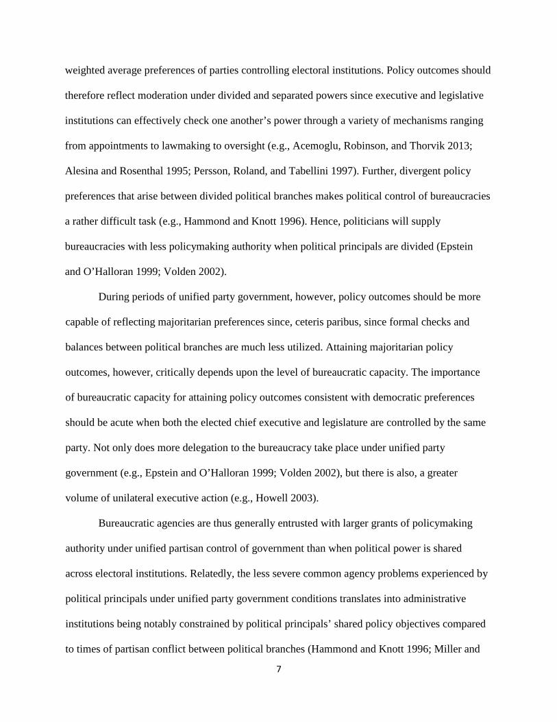
Patty 2013), and constructing a favorable agency reputation through innovation and cultivating
professional networks within relevant occupational fields (Carpenter 2001). When bureaucrats
have neither sufficient incentives’ nor means to acquire expertise, they are constrained in
effectively administering policy. Under such circumstances, they will either shirk by not
following prescribed policies, or be unable to adhere to the policy wishes of their political
principals.
The preceding discussion underscores the importance of bureaucratic capacity for
effective governance. Yet, the link between democratic politics and administration is also crucial
for understanding the extent to which policy outcomes reflect what elected officials want. Francis
Fukuyama (2013: 364) notes that the interaction between bureaucratic capacity and discretion
ultimately determine governance quality.2 Governance quality can be defined as the extent to
which administrative actors can execute the policy goals of their political principals (Fukuyama
2013: 350). This linkage is consistent with the notion that as bureaucracies become more
professionalized (i.e., capacity rises), they seek greater autonomy as a requisite for exercising their
expertise (Miller and Whitford 2016: 167).
Unlike standard separation of powers accounts whose central focus is on the institutional
battle over which governmental branch is afforded policymaking authority (e.g., delegation and
discretion in lawmaking and agency rulemaking), the aim of this study is to focus on policy
outcomes. Under a divided party government scenario, policy outcomes should reflect the
2 Fukuyama’s (2013: Figure 3, 362) conceptualization of bureaucratic autonomy is narrowly
restricted to the relative reliance on discretion vis-à-vis rules (cf. Carpenter 2001 for both a
broader and distinct definition of bureaucratic autonomy). See also, Note 1.
7
weighted average preferences of parties controlling electoral institutions. Policy outcomes should
therefore reflect moderation under divided and separated powers since executive and legislative
institutions can effectively check one another’s power through a variety of mechanisms ranging
from appointments to lawmaking to oversight (e.g., Acemoglu, Robinson, and Thorvik 2013;
Alesina and Rosenthal 1995; Persson, Roland, and Tabellini 1997). Further, divergent policy
preferences that arise between divided political branches makes political control of bureaucracies
a rather difficult task (e.g., Hammond and Knott 1996). Hence, politicians will supply
bureaucracies with less policymaking authority when political principals are divided (Epstein
and O’Halloran 1999; Volden 2002).
During periods of unified party government, however, policy outcomes should be more
capable of reflecting majoritarian preferences since, ceteris paribus, since formal checks and
balances between political branches are much less utilized. Attaining majoritarian policy
outcomes, however, critically depends upon the level of bureaucratic capacity. The importance
of bureaucratic capacity for attaining policy outcomes consistent with democratic preferences
should be acute when both the elected chief executive and legislature are controlled by the same
party. Not only does more delegation to the bureaucracy take place under unified party
government (e.g., Epstein and O’Halloran 1999; Volden 2002), but there is also, a greater
volume of unilateral executive action (e.g., Howell 2003).
Bureaucratic agencies are thus generally entrusted with larger grants of policymaking
authority under unified partisan control of government than when political power is shared
across electoral institutions. Relatedly, the less severe common agency problems experienced by
political principals under unified party government conditions translates into administrative
institutions being notably constrained by political principals’ shared policy objectives compared
to times of partisan conflict between political branches (Hammond and Knott 1996; Miller and

8
Whitford 2016: 167). A politically constrained bureaucracy that is entrusted with considerable
authority is therefore most consequential for determining governance quality in line with
Fukuyama’s (2013: 350) definition of this concept. We predict that bureaucratic capacity should
be positively associated with governance quality during times of unified party government. Next,
we apply this logic in the highly salient policy realm where sharp differences over policy
outcomes exist between partisan politicians: explaining market income variations among affluent
citizens in the American states.
Partisan Politics of Income Distribution: A View from the American States
The tide of rising income inequality observed in recent decades, both in the United States
and developed democracies around the world, is attributed to the sharp income gains for the most
affluent citizens (e.g., Atkinson and Piketty 2010; Leigh 2007; Piketty and Saez 2003, 2006;
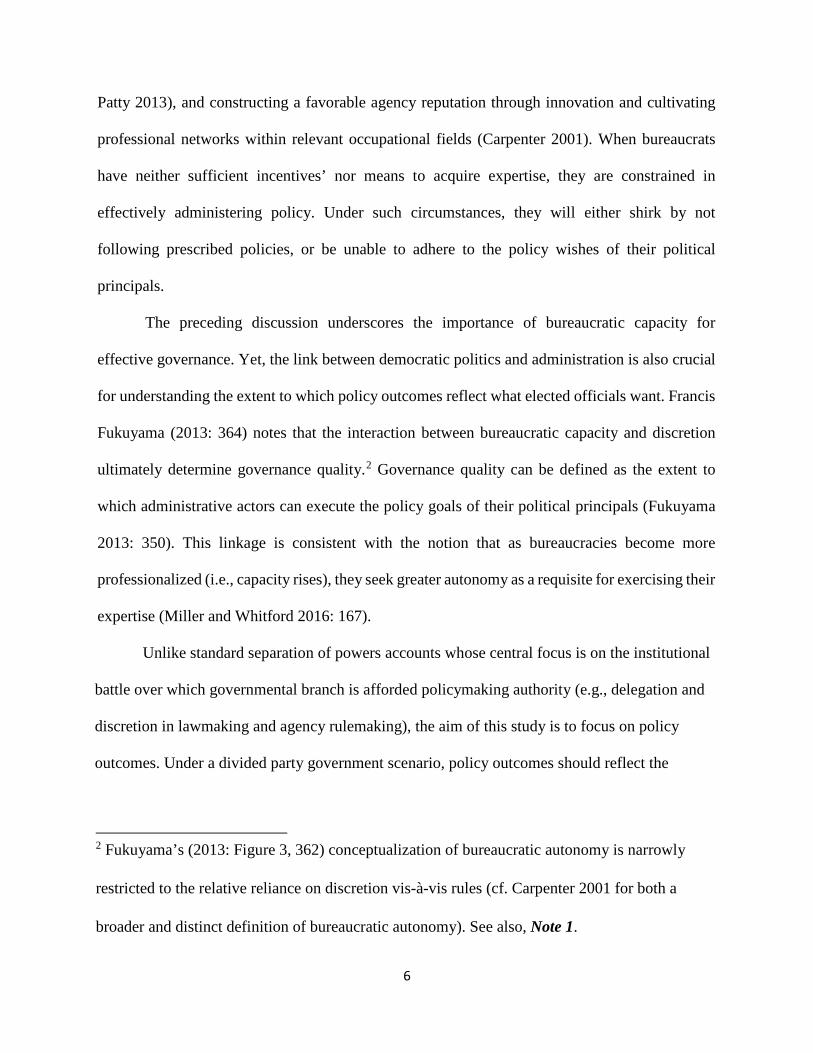
Scheve and Stasavage 2009). Figure 1 illustrates this pattern for the United States: it plots the
logged first−difference percentage change in real average adjusted gross household income
(AGI) based on IRS tax return data between 1986 and 2008 for each of the top six income
fractiles spanning the richest 10% of the income distribution (Sommellier and Price 2014; see
also Piketty and Saez 2012).3 These data constitute the pre−fiscal redistribution market income
since personal current transfer receipts are excluded, capital income is included, and modest
upward adjustments are made for income deductions relating to various personal individual
contributions to pensions and retirement plans, health saving accounts, plus moving expenses
3 Sommellier and Price (2014) compute state−level real adjusted gross income (AGI) data based
on national data on IRS tax returns generated by Piketty and Saez (2012).
9
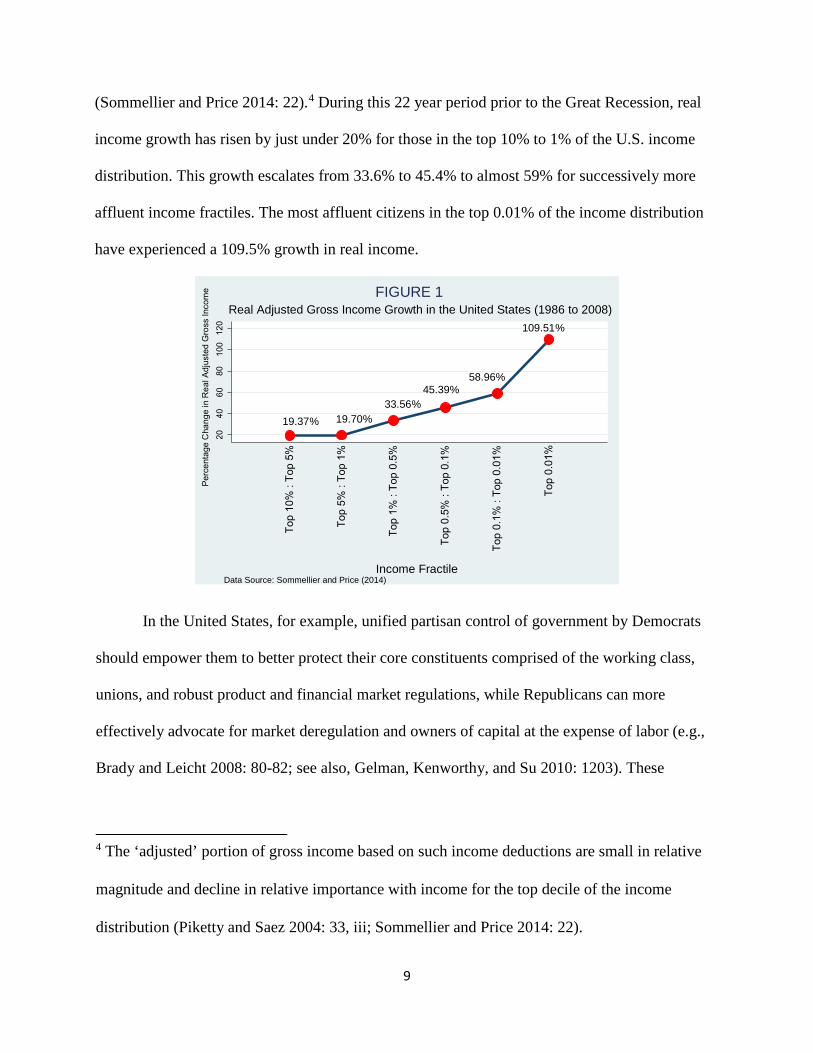
(Sommellier and Price 2014: 22).4 During this 22 year period prior to the Great Recession, real
income growth has risen by just under 20% for those in the top 10% to 1% of the U.S. income
distribution. This growth escalates from 33.6% to 45.4% to almost 59% for successively more
affluent income fractiles. The most affluent citizens in the top 0.01% of the income distribution
have experienced a 109.5% growth in real income.
In the United States, for example, unified partisan control of government by Democrats
should empower them to better protect their core constituents comprised of the working class,
unions, and robust product and financial market regulations, while Republicans can more
effectively advocate for market deregulation and owners of capital at the expense of labor (e.g.,
Brady and Leicht 2008: 80-82; see also, Gelman, Kenworthy, and Su 2010: 1203). These
4 The ‘adjusted’ portion of gross income based on such income deductions are small in relative
magnitude and decline in relative importance with income for the top decile of the income
distribution (Piketty and Saez 2004: 33, iii; Sommellier and Price 2014: 22).
% 19.37 % 19.70 33.56 %
58.96 % 45.39 %
109.51 %
Income Fractile
Real Adjusted Gross Income Growth in the United States (1986 to 2008) FIGURE 1
Data Source: Sommellier and Price (2014)
10
partisan differences are rooted in a starkly opposed understanding of the basic relationship
between inequality and economic growth. For instance, a leading liberal economist, Nobel
Laureate Joseph Stiglitz, asserts that “Increasing Inequality means a weaker economy, which
means increasing inequality, which means a weaker economy.” (Lowery 2012). Conversely,
conservative economists such as the Heritage Foundation’s Rea S. Hederman view “the problem
is that the policies that encourage growth also encourage inequality.” (Lowery 2012). Partisan
differences should be reflected in the distribution of income – most notably, the income of the
affluent segment of society. This is because partisan differences should be greatest at either end
of the income distribution since both parties must compete for the median (income) voter (see
Meltzer and Richard 1981). However, converting partisan policy preferences into actual policies
requires sufficient control by a single political party (Barrilleaux, Holbrook and Langer 2002).
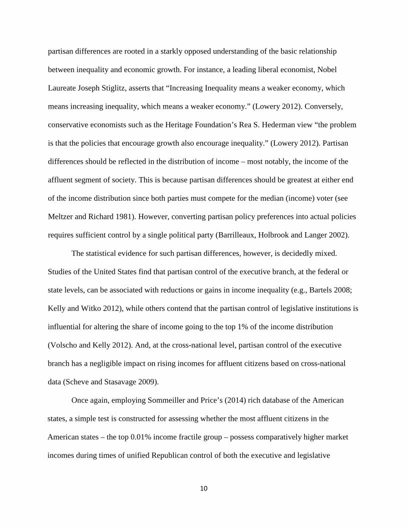
The statistical evidence for such partisan differences, however, is decidedly mixed.
Studies of the United States find that partisan control of the executive branch, at the federal or
state levels, can be associated with reductions or gains in income inequality (e.g., Bartels 2008;
Kelly and Witko 2012), while others contend that the partisan control of legislative institutions is
influential for altering the share of income going to the top 1% of the income distribution
(Volscho and Kelly 2012). And, at the cross-national level, partisan control of the executive
branch has a negligible impact on rising incomes for affluent citizens based on cross-national
data (Scheve and Stasavage 2009).
Once again, employing Sommeiller and Price’s (2014) rich database of the American
states, a simple test is constructed for assessing whether the most affluent citizens in the
American states – the top 0.01% income fractile group – possess comparatively higher market
incomes during times of unified Republican control of both the executive and legislative
11
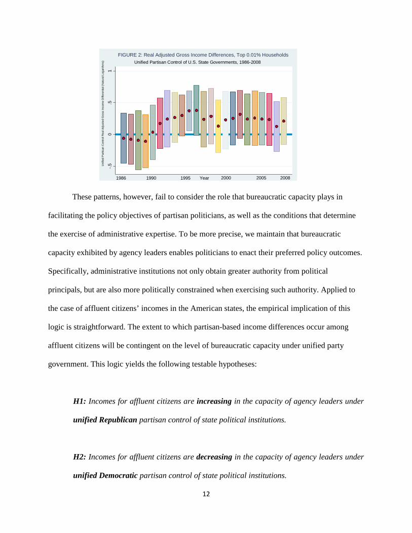
branches versus periods of unified Democratic control of these electoral institutions.5 Figure 2
depicts the results of this simple test: the cranberry dots are the estimated average difference in
logged income for the top 0.01% income fractile group for unified Republican states versus
unified Democratic states (the surrounding bars denote the corresponding 95% confidence
intervals). Excluding the 1994−1996 period, income for the most affluent citizens in the United
States is not significantly higher under unified Republican state governments’ relative to unified
Democratic state governments. In tandem, Figures 1 and 2 generally indicate an absence of a
statistical association between surging incomes of the most affluent citizens and unified partisan
control of U.S. state governments.5 This empirical disconnect top earners’ incomes and which
political party controls state government is corroborated in more sophisticated statistical tests
(see Supporting Information, Section 1. Additional Evidence of Null Effects for Unified Partisan
Control of State Government).
5 These estimates are based on a series of cross−section state−level regressions per annum (N =
49) estimating the effects of unified Democratic partisan control and unified Republican partisan
control as binary indicators (divided partisan control is captured in the intercept term) on the
natural logarithm of the real average AGI for the most affluent citizens (Top 0.01%).
12
These patterns, however, fail to consider the role that bureaucratic capacity plays in
facilitating the policy objectives of partisan politicians, as well as the conditions that determine
the exercise of administrative expertise. To be more precise, we maintain that bureaucratic
capacity exhibited by agency leaders enables politicians to enact their preferred policy outcomes.
Specifically, administrative institutions not only obtain greater authority from political
principals, but are also more politically constrained when exercising such authority. Applied to
the case of affluent citizens’ incomes in the American states, the empirical implication of this
logic is straightforward. The extent to which partisan-based income differences occur among
affluent citizens will be contingent on the level of bureaucratic capacity under unified party
government. This logic yields the following testable hypotheses:
H1: Incomes for affluent citizens are increasing in the capacity of agency leaders under
unified Republican partisan control of state political institutions.
H2: Incomes for affluent citizens are decreasing in the capacity of agency leaders under
unified Democratic partisan control of state political institutions.
-.50
.51
Uni
fied
Par
tisan
Con
trol R
eal A
djus
ted
Gro
ss In
com
e D
iffer
entia
l (N
atur
al L
ogar
ithm
s) Unified Partisan Control of U.S. State Governments, 1986-2008FIGURE 2: Real Adjusted Gross Income Differences, Top 0.01% Households
1986 1990 1995 2000 2005 2008Year
13
Put simply, affluent citizens’ incomes should be moving in the respective (i.e., opposite)
directions of what Republican and Democratic politicians want when each party controls both
the governor and state legislature as bureaucratic capacity is increasing. Therefore, we should
only observe partisan income differences consistent with left-right party policy preferences when
agency leaders’ capacity is sufficiently high.
It is important to note that because this study draws on Fukuyama’s (2013) definition of
governance quality, we thus focus on the role bureaucratic capacity plays in shaping partisan
income differences among affluent citizens. Recent research by Boushey and McGrath (2017)
has made an important contribution to our understanding of how differences in the capacities of
the legislative and executive branches can impact policy delegation in the realm of rulemaking
activities. Our study complements the policy consequences of separation of powers between
political branches by highlighting the critical role agency leadership plays when it comes to
converting democratic preferences into policy outcomes.
Research Design, Data, and Econometric Methods
Our hypotheses are tested using panel data on the average state−level real adjusted real
gross income (ARGI) reported on IRS tax returns within a given income fractile group among the
top decile of the income distribution covering 1986-2008 (Sommeiller and Price 2014).6 As
6 Because these IRS tax data are not available for the 1983−1985 period (see Sommeiller and
Price 2014: 9, Figure A), we begin the temporal sample with 1986 data. We end our temporal
sample in 2008 due to the sizable (and anomalous) economic shocks that occurred in late 2008.
We thank Estelle Sommeiller for generously making her data available to us.
14
noted earlier, the ARGI−IRS measures account for market income derived from various sources
noted earlier (Piketty and Saez 2003, 2004, 2006, 2012; Sommeiller and Price 2014: 21−22).7
These income measures are not available for lower income groups, and hence, we are only able
to test the empirical implications of our logic stated in H1 and H2 among affluent citizens. This
is not problematic since income inequality and dispersion in recent decades has been largely
driven by surges in the upper end of the income distribution, as documented in the preceding
section. Further, the ARGI−IRS type measure adopted here is preferable to Current Population
Survey (CPS) which suffers from underestimation of incomes in the top decile due to top-coding,
under-coverage, and under-reporting (Burkhauser et al.; 2012: 371-372).8
The state average ARGI measures are comprised of the following six fractiles: High
Affluent Citizens (the top 0.5% in a given state−year) – Top 0.01% in a given state−year (Mean =
7 The minor upward ‘adjustments’ made in AGI are due to income deductions ranging from
individual retirement accounts to moving expenses (Sommeiller and Price 2014: 22).
8 Although the CPS data underestimates income for the upper 10% of the income distribution,
Burkhauser, et al. (2012) note that the ARGI-IRS and CPS series trends also diverge when
analyzing the top 1%. Burkhauser, et al. (2012: 380) note that the ARGI−IRS data for the top 1%
are largely consistent with data from the Survey of Consumer Finance (SCF). The lone
exceptions reveal that the AGI−IRS data underestimates the large surge of income going to the
top 1% pre-1994 (Wolf and Zacharias 2009), while slightly overestimating income by less than
one percentage point for 2006 (Kennickell 2009). Therefore, the ARGI−IRS data represent an
unbiased estimate for the top 1% vis-à-vis the SCF data, while more accurately capturing
incomes of affluent citizens than the CPS data.
15
$13,501,708; SD = $11,569,395; Min = $1,532,994; Max = $90,882,595), Top 0.1% : Top
0.01% in a given state−year (Mean = $2,064,282; SD = $1,033,499; Min = $561,193; Max =
$8,276,840), Top 0.5% : Top 0.1% in a given state−year (Mean = $688,960; SD = $255,357;
Min = $291,246; Max = $2,158,379); and Low Affluent Citizens (between the top 10% and to
0.5% in a given state−year) – Top 1% : Top 0.5% in a given state−year (Mean = $372,922; SD =
$111,513; Min = $200,829; Max = $999,981), Top 5%: Top 1% in a given state−year (Mean =
$186,889; SD = $40,051; Min = $116,372; Max = $395,026), Top 10%: Top 5% in a given
state−year (Mean = $119,411; SD = $19,637; Min = $81,569; Max = $183,104). In addition,
considerable variations exist for real income growth across the American states. For example,
during the 1979−2007 period, Sommelier and Price (2014: 7, Table 1) demonstrate that the Top
1% fractile experienced a real income growth surge of nearly 415% in Connecticut (maximum),
163.5% in South Carolina (median rank), and 74% in West Virginia (minimum).
Unified partisan control of both governors and the legislature is critical given that each
party’s ability to obtain their preferred policy outcomes requires interbranch coordination in a
separation of powers system. Unified Republican Control (URC) is equal to 1 when both the
Governor and both legislative chambers are controlled by this party for a given state−year, and
equal to zero otherwise (Mean = 0.29, SD = 0.45). Unified Democratic Control (UDC) is equal
to 1 when both the Governor and both legislative chambers are controlled by this party for a
given state−year, and equal to zero otherwise (Mean = 0.24, SD = 0.43). Divided Partisan
Control is captured in the intercept term for each statistical model (Mean = 0.47, SD = 0.50).
To measure the concept of bureaucratic capacity for agency leaders we utilize a
professionalism based measure based on executive agency head salary compensation recently
proposed by Boushey and McGrath (2017). Boushey and McGrath (2017: 92) note that
compensation yields expertise, and hence it will be more difficult to recruit quality personnel
16
who are willing to remain in an agency and cultivate expertise (Gailmard and Patty 2013;
Teodoro 2013). The importance of attracting and retaining a professionalized, skilled public
sector workforce is embodied in the charters of state political compensation commissions
(Boushey and McGrath 2017: 90). Conceptually, the executive agency head compensation
measure that we adopt is compatible with the perspective that “… in modern organizations we
trust highly educated professionals with a much higher degree of discretion because we assume
or hope that they will be guided by internal norms in cases where behavior cannot be monitored
from the outside.” (Fukuyama 2013: 354). Fixed salary-based measures possess strong
convergent validity in several field experiments in settings outside the United States.9 For
instance, Dal Bó, Finan, and Rossi (2013) field experiment analyzing the filling of civil service
positions in distressed Mexican municipalities reveals that those governments offering higher
salaries attract superior ‘talent’ based on higher scores related to job market performance.
Relatedly, Ashraf, Bandiera, and Lee’s (2016) field experiments for civil service recruitment in
Zambia finds that higher wages attract “go-getters” whom are more effective in implementing
governments’ adopted policies consistent with politicians’ preferences, while lower wages attract
“do-gooders” whom exhibit a stronger, albeit much broader, public service motivation.
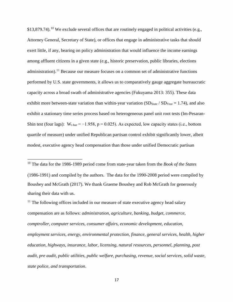
Bureaucratic Capacity is measured as the median 2000 constant-dollar adjusted salary
compensation for major state agency heads across 34 high-level executive offices that pertain to
major administrative functions of each state for a given year (Mean = $ 84,546.10, SD =
9 For skepticism of performance-based pay incentives (as opposed to fixed salary-based
payments) in Danish central governments, see Binderkrantz and Christensen (2012).
17
$13,879.74).10 We exclude several offices that are routinely engaged in political activities (e.g.,
Attorney General, Secretary of State), or offices that engage in administrative tasks that should
exert little, if any, bearing on policy administration that would influence the income earnings
among affluent citizens in a given state (e.g., historic preservation, public libraries, elections
administration).11 Because our measure focuses on a common set of administrative functions
performed by U.S. state governments, it allows us to comparatively gauge aggregate bureaucratic
capacity across a broad swath of administrative agencies (Fukuyama 2013: 355). These data
exhibit more between-state variation than within-year variation (SDState / SDYear = 1.74), and also
exhibit a stationary time series process based on heterogeneous panel unit root tests (Im-Pesaran-
Shin test (four lags): Wt-bar = −1.958, p = 0.025). As expected, low capacity states (i.e., bottom
quartile of measure) under unified Republican partisan control exhibit significantly lower, albeit
modest, executive agency head compensation than those under unified Democratic partisan
10 The data for the 1986-1989 period come from state-year taken from the Book of the States
(1986-1991) and compiled by the authors. The data for the 1990-2008 period were compiled by
Boushey and McGrath (2017). We thank Graeme Boushey and Rob McGrath for generously
sharing their data with us. 11 The following offices included in our measure of state executive agency head salary
compensation are as follows: administration, agriculture, banking, budget, commerce,
comptroller, computer services, consumer affairs, economic development, education,
employment services, energy, environmental protection, finance, general services, health, higher
education, highways, insurance, labor, licensing, natural resources, personnel, planning, post
audit, pre audit, public utilities, public welfare, purchasing, revenue, social services, solid waste,
state police, and transportation.

18
control (MeanURC = $65,602, MeanUDC = $68,942, p = 0.000). High capacity unified Republican
control states (i.e., top quartile of measure) exhibit slightly less relative capacity compared to
unified Democratic control states (MeanURC = $101,527, MeanUDC = $103,075, p = 0.185).
Figure 3 provides a summary graphical portrait of these data with Box-Whisker plots. At
the poles, the states with the lowest median executive agency head salary compensation are
typically less populous states. For instance, Montana has the lowest median level of executive
agency head salary compensation while California’s is the largest between 1986-2008.
Tennessee is at the median value of executive agency head salary compensation during this
period. Yet, because abundant within-state variation exists and it is not merely a function of time,
these data exhibit interesting panel variations. For example, it is worth noting that eight southern
states are above the grand state median value of executive agency head salary compensation,
including states such as South Carolina, Georgia, and Virginia. Generally, states exhibiting either
low or high executive agency head compensation values tend to exhibit less within-state
temporal variation compared to those states that lie in the interquartile range of states.
We also control for other covariates that may also explain income variations among
affluent citizens in the American states. Changes in income among affluent citizens in the
American states may also be a function of marginal tax rates (Saez, Slemrod, and Giertz 2012).
To address this potential confounder, each statistical model contains a panel-based covariate,
Marginal Tax Rate (Mean = 0.0658, SD = 0.0176), that represents the estimated dynamic
marginal tax rates for a given state-year based on the methodology advanced by Reed, Rogers,
19
and Skidmore (2011).12 Controlling for state marginal tax rates as a potential confounder ensures
that the effects of bureaucratic capacity under alternative partisan government regimes is
independent of taxation policies.
12 The procedure implemented here was proposed by Reed, Rogers, and Skidmore (2011). This
method derives a between (state) and within (time) varying measure of marginal tax rates for
American states. This measure estimates each state’s average marginal tax rate for a given year
using corporate income taxes, personal income taxes, sales taxes, property taxes and all other
remaining taxes, and then subsequently aggregates the estimates from each of these five
components into an overall index. Personal income data come from the Bureau of Economic
20
Besides this potential state marginal tax rate confounder, additional ancillary control
variables are modeled to represent factors that often correlate to income for affluent citizens in
the American states. State Real Per Capita Income (Mean = $ 28,776, SD = $ 5,192, Min = $
17,080, Max = $ 49,581) is expected to exert a positive impact on a state’s affluent citizens’
incomes since richer (poorer) states tend to have more (less) affluent citizens for a given level of
citizen affluence represented by their respective income fractile group. Non−Farm Income Share
Analysis, http://www.bea.gov/iTable/index_regional.cfmstate; the source for state tax revenues
and state and local tax revenue (which include personal income tax revenue, corporate income
tax revenue, sales tax revenue, property tax revenue, and total tax revenue) is
http://www2.census.gov/pub/outgoing/govs/special60/, then download “Govt Finances.zip;” the
source for average marginal tax rates (including marginal tax rates on wages, dividend income
and pension income) is NBER TAXSIM (http://users.nber.org/~taxsim/marginal-tax-rates/),
corporate income tax (including the number of corporate income tax brackets and the maximum
statutory tax rate on corporate profits) comes from the Tax Foundation
(http://taxfoundation.org/article/state-corporate-income-tax-rates); sales tax data (including the
overall state-level sales tax rate and the state-level tax on food: via Council on State
Governments, Knowledge Center ( http://knowledgecenter.csg.org/kc/category/content-
type/bosarchive); and, property tax revenues (DC Office of Revenue Analysis:
http://cfo.dc.gov/page/taxburdens-comparison).
21
(Mean = 0.994, SD = 0.018, Min = 0.902, Max = 1.06813) should be positively related to affluent
citizens’ income for a given level of citizen affluence. States that derive a larger share of total
income from agriculture possess affluent citizens with lower income levels compared to their
counterparts in states that derive a larger share of their income from manufacturing or
technology. Use of these income−related measures ensures that any impacts attributable to the
state capacity measure are independent of income effects.13 State Citizen Ideology (Berry, et al.
1998) may influence income for affluent citizens as a potential confounding factor with the
partisan control of government (Mean = 50.84, SD = 15.03, Min = 8.45, Max = 95.97).14
Because income redistribution is more tightly linked when the median voter is left−leaning
(Kenworthy and Pontusson 2005), states comprised of more liberal (conservative) citizens will
be associated with lower (higher) income for their affluent citizens, ceteris paribus. Inclusion of
this covariate should yield conservative estimates of the main theoretical hypotheses of interest
13 Non−farm income shares exceeding 1.0 imply that farm income is negative due to negative
proprietor’s farm income estimates. We thank Jeff Newman at BEA for this insight (e−mail
correspondence: Jeff Newman, Bureau of Economic Analysis, Tuesday, February 19, 2013).
13 One can infer that changes in state capacity measure are driven by changes in the denominator
relating to state total personal income, and not the size and scope of government. Controlling for
income effects ensures avoiding the spurious regression problem.
14 This state citizen ideology measure is based on computing congressional candidates’ ideology
using the method described in Berry, et al. (1998: 330−331) and these data were obtained via
Richard C. Fording’s website (http://www.bama.ua.edu/~rcfording/stateideology.html,
ideo6008.xslx, citi6008 variable).
22
given the extra variation due to electoral changes captured by this measure will better account for
income shifts that may otherwise be falsely attributed to discrete unified partisan control shifts.
The methodological approach adopted here is to estimate a series of first−order
autoregressive distributed lag panel regression models using both time and state fixed effects.15
In addition, we compare the robustness of the model specifications reported in the manuscript to
those based on a generalized ARDL(1,1)-ECM approach that accounts for distinct short and
long−run relationships (e.g., see Kelly and Witko 2012).16 Although the estimates (and
corresponding precision) vary somewhat, the total long-run marginal effect results from this
alternative dynamic model specification offer substantively similar support for H1 and H2
compared to the evidence presented in the next section based on a more parsimonious approach
that is desirable given the stationarity properties of the Bureaucratic Capacity documented
earlier in this section.
15 Estimation of equation (1) by use of OLS is not problematic in panels with sufficiently large
number of time points because Nickell (1981) bias is sufficiently small in short T panel designs.
However, the solution of instrumental variables to account for Nickell bias result in a sharp
tradeoff between bias and efficiency as T increases in size (Wawro 2002: 38). Beck and Katz’s
(2011: 342) Monte Carlo evidence demonstrates the advantages of OLS estimation in the
presence of lagged dependent variables with T ≥ 20 (our study contains a T = 23) compared to
instrumental estimation approaches.
16 See Supporting Information document (2. Robustness Checks: Comparison of Reported
Model Results to Alternative Model Specifications and Functional Forms section).
23
Both unobserved state−level and temporal heterogeneity are accounted for by specifying
two−way fixed effects in all model specifications. This aspect of our identification strategy is
critical for our substantive problem so as to ensure that the estimates are not confounded by
omitted variable bias attributable to common national government forces or unobserved
timeinvariant state−level variations, as well as allowing for meaningful comparisons both across
states and time. Further, the two−way fixed effects modeling approach allows for direct
relationship comparisons, for example, between unified Democratic control of state government
in Alabama in 1993 with unified Democratic control of state government in California in 2003.
The general form of the statistical model specification employed is:
( ) ( ) ( )
( )
, 0 1 , 1 1 , 1 2 , 1 3 , 1 4 , 1
5 , 1 , 1 6 , 1 7 , 1 , 1, 1
8 , 1 , 1 ,, 1
(1)
pi t i t i t i t i t i t
pi t i t i t i t i ti t
pi t k k i t i i t t i ti t
ARGI ARGI URC UDC BC BC
URC BC URC BC UDC BC
UDC BC Z S T
α α β β β β
β β β
β γ ψ η ε
− − − − −
− − − − −−
− −−
= + + + + +
+ × + × + ×
+ × + + + +
The dependent variable ARGI i, t is the adjusted gross real income by household for state i in year
t (see Sommeillier and Price 2014. URC i, t is unified Republican control in state i and year t,
UDC i, t is unified Democratic control in state i and year t, BC pi, t represents the pth higher-order
polynomial of Bureaucratic Capacity in state i and year t, Z k i, t consists of a kth vector of
ancillary control variables in state i and year t, Si is a vector of state−level fixed effects, Tt is a
vector of time fixed effects, and ε i, t is a residual term. The covariates are modeled as operating
on a one-year lag effect on affluent citizens’ market incomes since both policy and
implementation lags will necessarily create temporal friction in the conversion of political and
policy conditions into policy outcomes. The pth higher-order polynomial of Bureaucratic
Capacity covariates account for potential nonlinearities present for the conditional interaction
24
effects for various partisan control regimes. If such nonlinearities are not present in these data,
then these terms are excluded from the relevant model specifications.17
Recalling equation (1), the total long-run marginal effect of unified Republican partisan
control on affluent citizens’ incomes relative to the divided partisan control baseline is: ([β1 + β5
× BCi,t−1 + β6 × BCp i,t−1] / [1 − α1]), where evidence of H1 occurs when (β5 + β6 ) / [1 − α1] > 0.
That is, bureaucratic capacity has the long-term marginal effect of increasing affluent citizens’
incomes when major political branches are controlled by the Republican party. Similarly, the
total long-run marginal effect of unified Democratic partisan control on affluent citizens’
incomes relative to the divided partisan control baseline is: ([β2 + β7 × BCi,t−1 + β8 × BCp i,t−1] /
[1 − α1]), where H2 obtains empirical support if (β7 + β8) / [1 − α1] < 0. Put simply, bureaucratic
capacity will translate into decreasing incomes for affluent citizens relative to the divided
partisan control baseline. Total long-run marginal income differences accrued between unified
Republican and unified Democratic regimes is given by {[β1 + β5 × BCi,t−1 + β6 × BCp i,t−1] / [1 −
α1]} – { [β2 + β7 × BCi,t−1 + β8 × BCp i,t−1] / [1 − α1]}. Next, the empirical findings are presented.
17 Robustness checks comparing the reported model results based on asymmetric linear-quadratic
conditional bureaucratic capacity effects compared to those based on either symmetric linear or
quadratic conditional bureaucratic effects provide substantively similar findings regarding the
core predictions by the theory. This information can be obtained in the Supporting Information
document (2. Robustness Checks: Comparison of Reported Model Results to Alternative Model
Specifications and Functional Forms section).
25
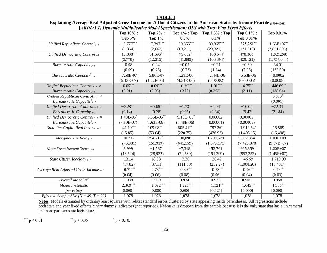
Empirical Findings
Table 1 reports the regression estimates for the statistical models that test the theory’s
predictions. One notices that the lack of statistical significance for the Bureaucratic Capacity
additive coefficients suggests that the level of executive agency head compensation in the
American states has little bearing on policy outcomes under divided partisan control of state
governments. For the highest income fractile (Top 0.01%), the pattern of coefficients associated
with Unified Republican Control covariates indicate that a U-shaped income surge for this group
that arises at sufficiently high levels of bureaucratic capacity. For the remaining five income
fractile models below the Top 0.01%, the positive and statistically significant coefficients for the
Unified Republican Control x Bureaucratic Capacity, coupled with the negative and statistically
significant coefficients for the Unified Democratic Control x Bureaucratic Capacity, offer
preliminary evidence that incomes are rising (falling) in a state’s level of executive agency head
compensation consistent with H1 and H2, respectively.
Direct evaluation of H1 requires analyses of the total marginal partisan income
differences under unified Republican control of state political institutions versus a baseline of
divided partisan control for a given income fractile group, conditional on varying levels of
bureaucratic capacity. If H1 is supported by these data, then income differences should be
upward sloping with respect to the bureaucratic capacity displayed by agency leaders. This is
graphically portrayed in Figure 4. Figure 4A displays the conditional average impact of
bureaucratic capacity on incomes for the most affluent subset of citizens (Top 0.01%) under
unified Republican partisan control regimes. Incomes are higher than the divided partisan control
baseline under very low levels of bureaucratic capacity before declining at moderate levels. What
is worth noting is that incomes noticeably surge when the bureaucratic capacity measure is at or
exceeds the 75th percentile value under such partisan regimes (πBC|URC ≥ 0.75). For instance,
26
TABLE 1 Explaining Average Real Adjusted Gross Income for Affluent Citizens in the American States by Income Fractile (1986−2008)
[ARDL(1,1) Dynamic Multiplicative Model Specification: OLS with Two−Way Fixed Effects] Top 10% :
Top 5% Top 5% : Top 1%
Top 1% : Top 0.5%
Top 0.5% : Top 0.1%
Top 0.1% : Top 0.01%
Top 0.01%
Unified Republican Control t−1 −3,777*** (1,354)
−7,397*** (2,663)
−30,855*** (10,211)
−80,365*** (29,321)
−375,251** (171,818)
1.66E+07** (7,801,395)
Unified Democratic Control t-1 12,838** (5,778)
31,595** (12,219)
79,662* (41,889)
−186,544* (103,894)
478,308 (429,122)
1,921,268 (1,757,644)
Bureaucratic Capacity t−1 0.08 (0.09)
0.04 (0.26)
−0.05 (0.73)
−0.21 (1.84)
−0.60 (7.96)
34.01 (133.50)
Bureaucratic Capacity2t−1 −7.50E-07
(5.43E-07) −5.86E-07 (1.62E-06)
−1.29E-06 (4.54E-06)
−2.44E-06 (0.00002)
−6.63E-06
(0.00005) −0.0002 (0.0008)
Unified Republican Control t−1 × Bureaucratic Capacity t−1
0.05*** (0.01)
0.09*** (0.03)
1.01*** (0.363)
4.75** (2.11)
−446.69** (188.64)
Unified Republican Control t−1 × Bureaucratic Capacity2
t−1 _________ _________ __________ ___________ __________ 0.003**
(0.001) Unified Democratic Control t−1 ×
Bureaucratic Capacity t−1 −0.28** (0.14)
−0.66** (0.28)
−1.73*
(0.96) −4.04* (2.34)
−10.04 (9.42)
−22.31 (21.84)
Unified Democratic Control t−1 × Bureaucratic Capacity2
t−1 1.48E-06* (7.80E-07)
3.35E-06** (1.63E-06)
9.18E−06* (5.48E-06)
0.00002 (0.00001)
0.00005 (0.00005)
__________
State Per Capita Real Income t−1 47.10*** (15.85)
109.98** (53.04)
505.41** (220.75)
787.26* (426.92)
1,912.54* (1,405.15)
16,569 (16,498)
Marginal Tax Rate t−1 10,212 (46,881)
294,216* (151,919)
730,098 (641,159)
1,799,579 (1,673,171)
7,807,354 (7,423,878)
1.09E+08 (9.07E+07)
Non−Farm Income Share t−1 9,999 (13,524)
−1,587 (28,932)
−7,348 (72,589)
153,761 (191,399)
965,359 (953,252)
1.20E+07 (1.45E+07)
State Citizen Ideology t−1
−13.14 (17.82)
18.58 (37.11)
−3.36 (111.50)
−26.42 (252.27)
−46.69 (1,008.20)
−1,710.90 (15,401)
Average Real Adjusted Gross Income t−1 0.71*** (0.04)
0.78*** (0.06)
0.69*** (0.08)
0.73*** (0.06)
0.76*** (0.04)
0.76*** (0.03)
Overall Model R2 0.938 0.939 0.934 0.922 0.905 0.858 Model F-statistic
[p−value] 2,369***
[0.000] 2,692***
[0.000] 1,228***
[0.000] 1,521***
[0.321] 1,649***
[0.000] 1,385***
[0.000] Effective Sample Size (N = 49, T = 22) 1,078 1,078 1,078 1,078 1,078 1,078
Notes: Models estimated by ordinary least squares with robust standard errors clustered by state appearing inside parentheses. All regressions include both state and year fixed effects binary dummy indicators (not reported). Nebraska is dropped from the sample because it is the only state that has a unicameral and non−partisan state legislature.
*** p ≤ 0.01 ** p ≤ 0.05 * p ≤ 0.10.
27
income rises by $1.75 million, on average, when bureaucratic capacity is at the 90th percentile
value in this type of partisan regime (πBC|URC = 0.90). The patterns for those affluent citizens
whose incomes fall below the Top 0.01% group reveal a strikingly similar pattern. Contrary to
their partisan preferences, incomes for a wide swath of affluent citizens during times of unified
Republican control of state institutions is significantly lower than compared to divided partisan
control eras when bureaucratic capacity is rather low (πBC|URC ≤ 0.10).18
Conversely, when executive agency head compensation is relatively high (πBC|URC ≥
0.75), incomes for these groups are significantly above what one observes during an era of
divided partisan control. Figure 4B reveals that the second most affluent group (Top 0.1%:
0.01%) experiences lower incomes by $97,394 (πBC|URC = Min) and $66,629 (πBC|URC = 0.10) at
lower levels of bureaucratic capacity. However, incomes are estimated to be $64,397 (πBC|URC =
0.75), $107,168 (πBC|URC = 0.90), and $202,247 (πBC|URC = Max) higher than compared to the
divided partisan control baseline, respectively. The change from the 10th to 90th percentile values
in bureaucratic capacity results in an income surge of $173,797 or 16.79% of a standard
deviation income change for this group.
18 The numerical values of the bureaucratic capacity measure (median 2000 constant-dollar
adjusted salary compensation for major state agency heads) are as follows: πBC|URC = Min
($58,495.88), πBC|URC = 0.10 ($64,972.61), πBC|URC = 0.25 ($72,187.58), πBC|URC = 0.50
($81,505.09), πBC|URC = 0.75 ($92,556.81), πBC|URC = 0.90 ($101,561), and πBC|URC = Max
($121,577.6); πBC|UDC = Min ($55,787.34), πBC|UDC = 0.10 ($68,187.74), πBC|UDC = 0.25
($75,185.36), πBC|UDC = 0.50 ($85,975.63), πBC|UDC = 0.75 ($93917.29), πBC|UDC = 0.90
($103,121.5), and πBC|UDC = Max ($123,879.8).
28
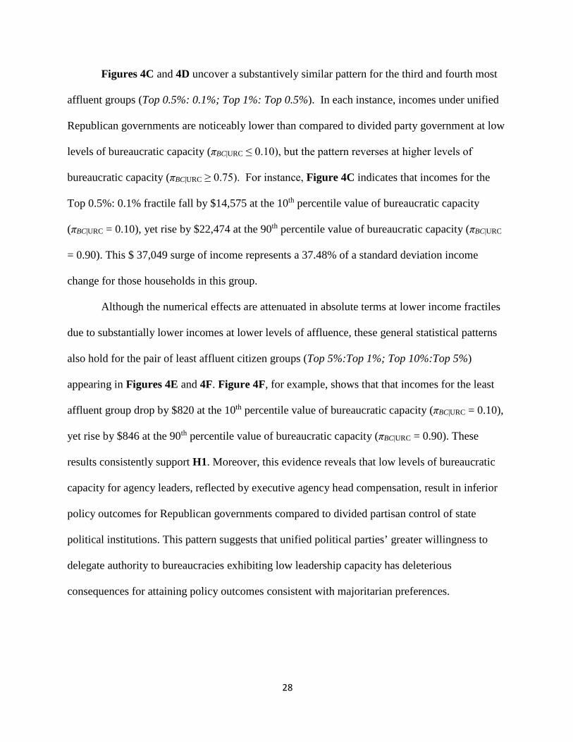
Figures 4C and 4D uncover a substantively similar pattern for the third and fourth most
affluent groups (Top 0.5%: 0.1%; Top 1%: Top 0.5%). In each instance, incomes under unified
Republican governments are noticeably lower than compared to divided party government at low
levels of bureaucratic capacity (πBC|URC ≤ 0.10), but the pattern reverses at higher levels of
bureaucratic capacity (πBC|URC ≥ 0.75). For instance, Figure 4C indicates that incomes for the
Top 0.5%: 0.1% fractile fall by $14,575 at the 10th percentile value of bureaucratic capacity
(πBC|URC = 0.10), yet rise by $22,474 at the 90th percentile value of bureaucratic capacity (πBC|URC
= 0.90). This $ 37,049 surge of income represents a 37.48% of a standard deviation income
change for those households in this group.
Although the numerical effects are attenuated in absolute terms at lower income fractiles
due to substantially lower incomes at lower levels of affluence, these general statistical patterns
also hold for the pair of least affluent citizen groups (Top 5%:Top 1%; Top 10%:Top 5%)
appearing in Figures 4E and 4F. Figure 4F, for example, shows that that incomes for the least
affluent group drop by $820 at the 10th percentile value of bureaucratic capacity (πBC|URC = 0.10),
yet rise by $846 at the 90th percentile value of bureaucratic capacity (πBC|URC = 0.90). These
results consistently support H1. Moreover, this evidence reveals that low levels of bureaucratic
capacity for agency leaders, reflected by executive agency head compensation, result in inferior
policy outcomes for Republican governments compared to divided partisan control of state
political institutions. This pattern suggests that unified political parties’ greater willingness to
delegate authority to bureaucracies exhibiting low leadership capacity has deleterious
consequences for attaining policy outcomes consistent with majoritarian preferences.
29
FIGURE 4
Analyzing Affluent Citizens’ Incomes Increasing in Bureaucratic Capacity under Unified Republican Governments in the American States (H1)
Notes: Long-run total marginal effect is computed as ([β1 + β5 × BCi,t−1 + β6 × BCp
i,t−1] / [1 − α1]) from Equation (1). The comparison baseline is divided partisan control of state governor and legislative branches. p = 1 (first-order polynomial) for all income fractiles except for Top 0.01% (where p = 2).
30
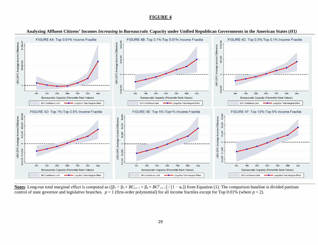
Figure 5 analyzes the total marginal partisan income differences under unified
Democratic control of state political institutions versus a baseline of divided partisan control for
a given income fractile group, conditional on varying levels of bureaucratic capacity. Consistent
with H2, a downward sloping relationship should exist between such income differences and
bureaucratic capacity. In the top panel of graphs (Figures 5A– 5C), although incomes among the
Top 0.5% affluent citizens generally declines in the level of bureaucratic capacity, these impacts
are modest compared to unified Republican partisan regimes and are also estimated with
considerable imprecision for the three most affluent groups.
For the three lower citizen affluence groups, the negative conditional impact of
bureaucratic capacity becomes more statistically discernible for reducing incomes of affluent
citizens under unified Democratic partisan control. For instance, incomes for the Top 1%: Top
0.5% (Figure 5D) change from $4,432 higher than the divided partisan control baseline when
bureaucratic capacity is at the 10th percentile value (πBC|UDC = 0.10) to $−1,038 lower at the 90th
percentile value (πBC|UDC = 0.90). This decline of $5,470 is equivalent to a 5.2% of a standard
deviation for incomes in this group. The relative magnitude effect of this substantially smaller
effect than the parallel effect under unified Republican partisan control in Figure 4D ($14,072 or
14.24% of a standard deviation for incomes in this group).
Although the statistical evidence supporting H2 is attenuated compared to H1, it
nonetheless reveals that rising bureaucratic capacity at lower levels is effective at reducing
incomes for the affluent only below the Top 0.5% of the income distribution when
Democratic politicians experience unified control of both the governor and legislature. Although
marginal increases in bureaucratic capacity from low to moderate levels is effective at reducing
incomes for affluent citizens, it fails to exert a parallel effect as one moves from moderate to

31
FIGURE 5
Analyzing Affluent Citizens’ Incomes Decreasing in Bureaucratic Capacity under Unified Democratic Governments in the American States (H2)
Notes: Long-run total marginal effect is computed as ([β2 + β7 × BCi,t−1 + β8 × BCp
i,t−1] / [1 − α1]), from Equation (1). The comparison baseline is divided partisan control of state governor and legislative branches. p = 2 (second-order polynomial) for all income fractiles except for Top 0.01% (where p = 1).
32
high levels of bureaucratic capacity. This asymmetric pattern may explain to some extent why
reducing income inequality is difficult for unified Democratic governments, even when
sufficiently high levels of executive agency head compensation ensures governance quality in
terms of converting partisan policy preferences into policy outcomes. Taken together,
bureaucratic capacity offers the most benefits for unified Republican governments in attaining
their preferred policy outcomes with respect to incomes among affluent citizens.
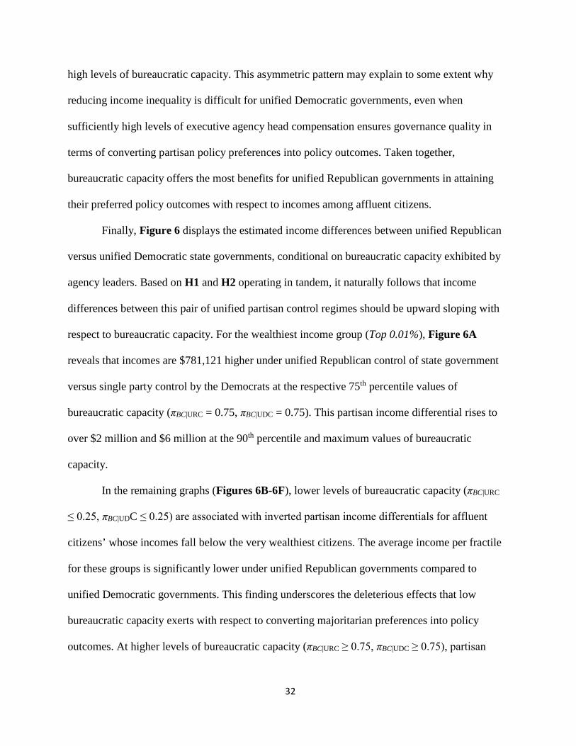
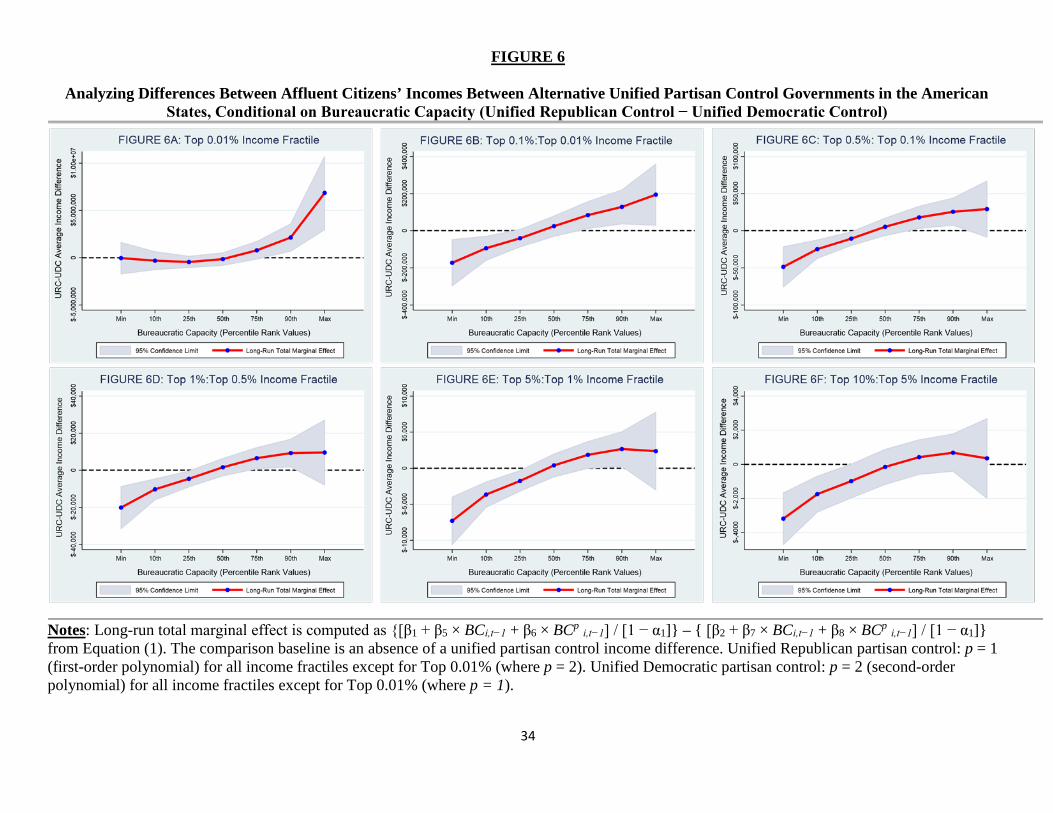
Finally, Figure 6 displays the estimated income differences between unified Republican
versus unified Democratic state governments, conditional on bureaucratic capacity exhibited by
agency leaders. Based on H1 and H2 operating in tandem, it naturally follows that income
differences between this pair of unified partisan control regimes should be upward sloping with
respect to bureaucratic capacity. For the wealthiest income group (Top 0.01%), Figure 6A
reveals that incomes are $781,121 higher under unified Republican control of state government
versus single party control by the Democrats at the respective 75th percentile values of
bureaucratic capacity (πBC|URC = 0.75, πBC|UDC = 0.75). This partisan income differential rises to
over $2 million and $6 million at the 90th percentile and maximum values of bureaucratic
capacity.
In the remaining graphs (Figures 6B-6F), lower levels of bureaucratic capacity (πBC|URC
≤ 0.25, πBC|UDC ≤ 0.25) are associated with inverted partisan income differentials for affluent
citizens’ whose incomes fall below the very wealthiest citizens. The average income per fractile
for these groups is significantly lower under unified Republican governments compared to
unified Democratic governments. This finding underscores the deleterious effects that low
bureaucratic capacity exerts with respect to converting majoritarian preferences into policy
outcomes. At higher levels of bureaucratic capacity (πBC|URC ≥ 0.75, πBC|UDC ≥ 0.75), partisan
33
income differentials are consistent with differences in partisan policy preferences regarding
incomes among affluent citizens. This difference ranges from a low of $422 (Figure 6F: πBC|URC
= 0.75, πBC|UDC = 0.75) to a high of $194,287 (Figure 6B: πBC|URC = Max, πBC|UDC = Max).
These findings clearly demonstrate that which party controls the reins of government
matters, yet such political influence in shaping policy outcomes relies heavily upon the caliber of
top level agency officials that are charged with providing leadership in state government
administration. When administrative institutions are weak, governance quality is low and policy
outcomes run counter to majoritarian preferences in a democracy. When public bureaucracies are
robust, they offer an effective mechanism for ensuring that policy outcomes are consistent with
the intention of elected officials operating under unified partisan governments.
Discussion
Speaking to the issue of policy execution in Federalist 70, Alexander Hamilton asserts
“And a government ill executed, whatever it may be in theory, must be in practice a bad
government.” (The Federalist Papers 1982: 355). Much of Hamilton’s advocacy of a robust
unified executive branch is rooted in the simple idea that effective governance requires not only
a unity of purpose, but also with the means of implementing this unity of purpose into action.
Speaking on the critical role required of effective administration in a democracy, Norton Long
(1949: 264) perceptively proscribed decades ago “Attempts to solve administrative problems in
isolation from the structure of power and purpose in the polity are bound to prove illusory.”
Motivated by these complementary insights regarding the fundamental tension of governance in
democracy offered by both Hamilton and Long, we seek to better understand the precise
conditions in which policy execution reflects the conversion of democratic preferences into
policy outcomes. We maintain that agency leaders serve as the focal point for understanding the
34
FIGURE 6
Analyzing Differences Between Affluent Citizens’ Incomes Between Alternative Unified Partisan Control Governments in the American States, Conditional on Bureaucratic Capacity (Unified Republican Control − Unified Democratic Control)
Notes: Long-run total marginal effect is computed as {[β1 + β5 × BCi,t−1 + β6 × BCp i,t−1] / [1 − α1]} – { [β2 + β7 × BCi,t−1 + β8 × BCp i,t−1] / [1 − α1]} from Equation (1). The comparison baseline is an absence of a unified partisan control income difference. Unified Republican partisan control: p = 1 (first-order polynomial) for all income fractiles except for Top 0.01% (where p = 2). Unified Democratic partisan control: p = 2 (second-order polynomial) for all income fractiles except for Top 0.01% (where p = 1).
35
nexus between politics and administration. Put simply, unity of purpose among elected officials
cannot guarantee policy success without the support of capable agency leaders.
Although we restrict our focus to the specific issue of analyzing whether politicians
effectively shape policy outcomes consistent with their own partisan agendas, this puzzle is
central to democratic governance since election outcomes and the resulting partisan composition
of political institutions should exert influence not only on policymaking activities, but also
resulting policy outcomes. We assert that the combination of unified party government and
sufficiently high levels of bureaucratic capacity displayed by agency leaders are required to
obtain policy outcomes consistent with majoritarian preferences. This logic presumes that the
successful execution of partisan politicians’ policy objectives requires entrusting considerable
policymaking authority into public agencies whom are led by high caliber leaders.
The empirical implications of this logic are analyzed by focusing on income variations
among several affluent income groups across the American states. These cases constitute an area
that not only clear partisan differences arise over policy outcomes (e.g., Bartels 2008; Brady and
Leicht 2008: 80−82; Gelman, Kenworthy, and Su 2010), but also that is most responsible for the
surge in income inequality experienced during the past several decades in the United States
(Piketty and Saez 2003; Sommeillier and Price 2014), and also around the world (e.g., Atkinson
and Piketty 2010; Leigh 2007; Piketty and Saez 2006). Analyzing the American states offers a
valuable setting to facilitate comparisons since these governments possess comparable macro-
structural features – i.e., mature democratic subnational systems operating under separated and
shared constitutional powers. In turn, this enables us to better isolate the conditions in which the
administrative state can effectively implement a partisan policy agenda on behalf democratic
institutions.
36
Following the lead of Boushey and McGrath (2017), we construct measures of
bureaucratic capacity displayed by agency leadership that are based on executive agency head
compensation in the American states for a common set of 34 line agencies. This measure is
intended to capture the incentives to invest in administrative expertise that mutually benefit
politicians and agencies. It is also a useful measure for gauging variations in bureaucratic
capacity among American states possessing strong infrastructural power (Mann 1984, 1988,
1993) since it gauges both spatial and temporal variation in resources and degree of
professionalization exhibited by top-level state agency leaders. However, it is important to
acknowledge that the present analyses are limited insofar that it cannot ascertain agency-specific
sources of contributing income gains/losses among affluent citizens, nor demarcate between
abridgement versus expansion efforts on behalf of state governments.19
The statistical evidence nonetheless shows that low levels of bureaucratic capacity
exhibited by agency leaders undermine elected officials’ efforts at attaining their policy goals
when the latter share common policy objectives. Lower levels of bureaucratic capacity often
yield lower market incomes for affluent citizens under unified Republican control of political
institutions, while the opposite condition happens under unified Democratic party governments.
Rising levels of bureaucratic capacity in the American states are generally associated with policy
outcomes that more closely cohere to politicians’ policy preferences when the Republican party
controls each of the major electoral branches of government than compared to when the
Democratic party possesses such unified control. Governance quality thus is at its apex when
politicians in separate branches have a unity of purpose, in conjunction with a highly capable
19 We thank an anonymous reviewer for raising this point.
37
administrative state that can effectively exercise the policymaking authority vested to them by
political institutions.
More broadly, bureaucratic capacity is not only normatively desirable for the mechanics
of administrative governance in mature, stable democracies, but also for executing the popular
will of majorities in these governmental systems. This is because public laws and executive
actions that have the force of policy are routinely interpreted and enforced by government
agencies. In recent decades, politicians and citizens’ groups alike have advocated efforts to
‘hollow out’ the administrative state for stated purposes of bringing about a closer connection
between democratic preferences and policy outcomes (e.g., Peters and Pierre 1998; Terry 2005).
Unfortunately, the logic and evidence presented in this study suggest that political efforts to
undermine the authority of the administrative state work at cross-purposes for obtaining policy
outcomes consistent with majoritarian preferences. Bureaucratic capacity, especially at the very
top level of government agencies, can therefore be viewed as a critical ingredient for enhancing
substantive representation over policy outcomes for those instances when a unity of purpose
exists among elected officials and the administrative state is not only entrusted with
policymaking authority, but also has sufficient means to exercise such power effectively.

38
References
Acemoglu, Daron, and James A. Robinson, and Ragnar Torvik. 2013. “Why Do Voters
Dismantle Checks and Balances?” Review of Economic Studies 80(July): 845−875.
Alesina, Alberto, and Howard Rosenthal. 1995. Partisan Politics, Divided Government, and the
Economy. New York: Cambridge University Press.
Ashraf, Nava, Oriana Bandiera, and Scott S. Lee. 2016. “Do-Gooders and Go-Getters: Selection
and Performance in Public Service Delivery.” Typescript. London School of Economics
and Political Science. June.
https://ashrafnava.files.wordpress.com/2016/07/dogoodersgogetters.pdf
Atkinson, Anthony B., and Thomas Piketty, eds. 2010. Top Incomes: A Global Perspective.
Oxford & New York: Oxford University Press.
Barrilleaux, Charles, Thomas M. Holbrook, and Laura Langer. 2002. “Electoral Competition,
Legislative Balance, and American Welfare State Policy.” American Journal of Political
Science 46(April): 415-427.
Bartels, Larry, M. 2008. Unequal Democracy: The Political Economy of the New Gilded Age.
Princeton, NJ: Princeton University Press.
Beck, Nathaniel, and Jonathan N. Katz. 2011. “Modeling Dynamics in Time-Series Cross-
Section Political Economy Data.” Annual Review of Political Science 14: 331-352.
Berry, William D., Evan J. Ringquist, Richard C. Fording, and Russell L. Hanson. 1998.
“Measuring Citizen and Government Ideology in the American States, 1960−1993.”
American Journal of Political Science 42(January): 327−348.
Berry, William D., Evan J. Ringquist, Richard C. Fording, Russell L. Hanson, and Carl E.
Klarner. 2010. “Measuring Citizen and Government Ideology in the American States: A
39
Re−Appraisal.” State Politics and Policy Quarterly 10(Summer): 117−135.
Besley, Timothy, and Torsten Persson. 2009. “The Origins of State Capacity: Property Rights,
Taxation, and Politics.” American Economic Review 99(September): 1218−1244.
Binderkrantz, Anne Skorkjaer, and Jorgen Gronnegaard Christensen. 2012. “Agency
Performance and Executive Pay in Government: An Empirical Test.” Journal of Public
Administration Research and Theory
Boushey, Graeme T., and Robert J. McGrath. 2017. “Experts, Amateurs, and Bureaucratic
Influence in the American States.” Journal of Public Administration Research and Theory
27(January): 85-103.
Brady, David, and Kevin T. Leicht. 2008. “Party to Inequality: Right Party Power and Income
Inequality in Affluent Western Democracies.” Research in Social Stratification and
Mobility 26(March): 77−106.
Burkhart, Richard V., Shuaizhang Feng, Stephen P. Jenkins, and Jeff Larrimore. 2012. “Recent
Trends in Top Income Shares in the United States: Reconciling Estimates from March
CPS and IRS Tax Return Data.” Review of Economics and Statistics 94(May): 371-388.
Carpenter, Daniel P. 2001. Forging Bureaucratic Autonomy: Reputations, Networks, and Policy
Innovation in Executive Agencies, 1862-1928. Princeton, NJ: Princeton University Press.
Carpenter, Daniel P. 2010. Reputation and Power: Organizational Image and Pharmaceutical
Regulation at the FDA. Princeton, NJ: Princeton University Press.
Carpenter, Daniel, and George A. Krause. 2012. “Reputation and Public Administration.” Public
Administration Review 72(January/February): 26-32.
Conlan, Timothy J. 1998. From New Federalism to Devolution: Twenty-Five Years of
Intergovernmental Reform. Washington, D.C.: Brookings Institution.
40
Dal Bó, Ernesto, Frederico Finan, and Martin A. Rossi. 2013. “Strengthening State Capabilities:
The Role of Financial Incentives in the Call of Public Service.” Quarterly Journal of
Economics 128(August): 1169-1218.
Downs, Anthony. 1967. Inside Bureaucracy. Boston, MA: Little Brown.
Dye, Thomas, R. 1990. American Federalism: Competition Among Governments. Lexington,
MA: Lexington Books.
Eisinger, Peter, K. 1988. The Rise of The Entrepreneurial State: State and Local Economic
Development Policy in the United States. Madison, WI: University of Wisconsin Press.
Epstein, David L., and Sharyn O’Halloran. 1999. Delegating Powers: A Transaction Cost
Politics Approach to Policymaking under Separated Powers. New York: Cambridge
University Press.
The Federalist Papers by Alexander Hamilton, James Madison, and John Jay. 1982. New York:
Bantam Books.
Fukuyama, Francis. 2013. “What is Governance?” Governance: An International Journal of
Policy, Administration, and Institutions 26(July): 347-368.
Gailmard, Sean, and John W. Patty. 2013. Learning While Governing: Expertise and
Accountability in the Executive Branch. Chicago, IL: University of Chicago Press.
Gelman, Andrew, Lane Kenworthy, and Yu-Sung Su. “Income Inequality and Partisan Voting in
the United States.” Social Science Quarterly 91(December): 1203-1219.
Hammond, Thomas H., and Jack H. Knott. 1996. “Who Controls the Bureaucracy? Presidential
Power, Congressional Dominance, Legal Constraints, and Bureaucratic Autonomy in a
Model of Institutional Policymaking.” Journal of Law, Economics, and Organization
12(May): 119-166.
41
Howell, William G. 2003. Power Without Persuasion: The Politics of Direct Presidential Action.
Princeton, NJ: Princeton University Press.
Huber, John D., Nolan McCarty. 2004. “Bureaucratic Capacity, Delegation, and Political
Reform.” American Political Science Review 98(August): 481-494.
Im, Kyung So, M. Hashem Pesaran, and Yongcheol Kim. 2003. “Testing for Unit Roots in
Heterogeneous Panels.” Journal of Econometrics 115(July): 53-74.
Kelly, Nathan J., and Christopher Witko. 2012. “Federalism and American Inequality.” Journal
of Politics 74(April): 414−426.
Kennickell, Arthur B. 2009. “Ponds and Streams: Wealth and Income in the U.S., 1989−2007.”
Federal Reserve Board Finance and Economic Discussion Series. No. 2009-13.
Kenworthy, Lane, and Jonas Pontusson. 2005. “Rising Inequality and the Politics of
Redistribution in Affluent Countries.” Perspectives on Politics 3(September): 449−471.
Krause, George A., and Neal D. Woods. 2014. “Policy Delegation, Comparative Institutional
Capacity, and Administrative Politics in the American States.” In Oxford Handbook of
State and Local Government, ed. Donald P. Haider-Markel, 363-396. New York: Oxford
University Press.
Langer, Laura. 2001. “The Consequences of State Economic Development Strategies on Income
Distribution in the American States, 1976-1994.” American Politics Research 29(July):
392-415.
Leigh, Andrew. 2007. “How Closely Do Top Income Shares Track Other Measures of
Inequality? Economic Journal 117(524): F619−F633.
Long, Norton E. 1949. “Power and Administration.” Public Administration Review 9(Autumn):
257-264.
42
Lowery, Annie. 2012. “Costs Seen in Income Inequality.” New York Times. October 17. Section,
Page: B1. http://www.nytimes.com/2012/10/17/business/economy/income-inequality-
may-take-toll-on-growth.html.
Mann, Michael. 1984. The Autonomous Power of the State. Oxford, UK: Blackwell.
Mann, Michael 1988. “The Autonomous Power of the State: Its Origins, Mechanisms, and
Results.” In States, War, and Capitalism: Studies in Political Sociology. Oxford, UK:
Blackwell. (Originally published in 1984. Archives Europeennes de Sociologie
25(November): 185-213).
Mann, Michael. 1993. The Sources of Social Power, Volume 2. Cambridge, UK: Cambridge
University Press.
Mikesell, John. 2007. “Changing State Capacity and Tax Effort in an Era of Devolving
Government, 1981−2003.” Publius: The Journal of Federalism 37(Fall): 532-550. Miller,
Gary J., and Andrew B. Whitford. 2016. Above Politics: Bureaucratic Discretion and
Credible Commitment. New York: Cambridge University Press.
Persson, Torsten, Gerard Roland, and Guido Tabellini. 1997. “Separation of Powers and Political
Accountability.” Quarterly Journal of Economics 112(November): 1163−1202.
Peters, B. Guy, and Jon Pierre. 1998. “Governance without Governing? Rethinking Public
Administration.” Journal of Public Administration Research and Theory 2(April): 223-
243.
Pfeffer, Jeffrey, and Gerald D. Salancik. 2003. The External Control of Organizations: A
Resource Dependence Perspective. Stanford, CA: Stanford University Press. Second
Edition.
43
Piketty, Thomas, and Emmanuel Saez. 2003. “Income Inequality in the United States, 1913−
1998.” Quarterly Journal of Economics 118(February): 1−39.
Piketty, Thomas, and Emmanuel Saez. 2004. “Income Inequality in the United States, 1913−
2002.” In Top Incomes over the Twentieth Century. Anthony B. Atkinson and Thomas
Piketty, editors. New York: Oxford University Press.
Piketty, Thomas, and Emmanuel Saez. 2006. “The Evolution of Top Incomes: A Historical and
International Perspective.” American Economic Review 96(June): 200−205.
Piketty, Thomas, and Emmanuel Saez. 2012. Downloadable Excel Files with 2012 data updates
to Tables and Figures in Piketty and Saez (2003):
http://elsa.berkeley.edu/~saez/TabFig2012.prel.xls.
Rainey, Hal G., and Paula Steinbauer. 1999. “Galloping Elephants: Developing Elements of a
Theory of Effective Government Organizations.” Journal of Public Administration
Research and Theory 9(January): 1-32.
Reed, W. Robert, Cynthia L. Rogers, and Mark Skidmore. 2011. “On Estimating Marginal Tax
Rates for U.S. States.” National Tax Journal 64(March): 59-84.
Rosen, Harvey. 2002. Public Finance. Sixth Edition. Boston: McGraw-Hill Irwin.
Scheve, Kenneth, and David Stasavage. 2009. “Institutions, Partisanship, and Inequality in the
Long Run.” World Politics 61(April): 215−253.
Saez, Emmanuel, Joel Slemrod, and Seth H. Giertz. 2012. “The Elasticity of Taxable Income
with Respect to Marginal Tax Rates: A Critical Review.” Journal of Economic Literature
50(March): 3−50.
Schneider, Saundra K., William G. Jacoby, and Jerrell D. Coggburn. 1997. “The Structure of

44
Bureaucratic Decision in the American States.” Public Administration Review
57(May/June): 240-249.
Simon, Hebert A. 1997. Administrative Behavior. Fourth Edition. New York: Free Press.
Soifer, Hillel. 2008. “State Infrastructural Power: Approaches to Conceptualization and
Measurement.” Studies in Comparative Institutional Development 43(December): 231-
251.
Sommeiller, Estelle, and Mark Price. 2014. The Increasingly Unequal States of America: Income
Inequality by State, 1917 to 2011. Economic Analysis and Research Network (EARN)
Report. http://www.epi.org/publication/unequal-states/
Stark, Kirk J. 2010. “Rich States, Poor States: Assessing the Design and Effect of a U.S. Fiscal
Equalization Regime.” Tax Law Review 63(Summer): 957-1008.
Teodoro, Manuel P. 2011. Bureaucratic Ambition: Careers, Motives, and the Innovative
Administrator. Baltimore, MD: Johns Hopkins University Press.
Terry, Larry D. 2005. “The Thinning of Administrative Institutions in the Hollow State.”
Administration & Society 37(September): 426-444.
U.S. Government Accountability Office (GAO). 2010. State and Local Governments: Fiscal
Pressures Could Have Implications for Future Delivery of Intergovernmental Programs.
Report to the Ranking Member, Committee on the Budget, House of Representatives.
Washington, D.C.: Government Accountability Office.
Volden, Craig. 2002. “A Formal Model of the Politics of Delegation in the Separation of
Powers System.” American Journal of Political Science 46(January): 111-133.
Volscho, Thomas W., and Nathan J. Kelly. 2012. “The Rise of the Super−Rich: Power
Resources, Taxes, Financial Markets, and the Dynamics of the Top 1 Percent,
45
1949−2008.” American Sociological Review 77(October): 679−699.
Wawro, Gregory. 2002. “Estimating Dynamic Panel Data Models in Political Science.” Political
Analysis 10(Winter): 25-48.
Wolff, Edward N., and Ajit Zacharias. 2009. “Household Wealth and the Measurement of
Economic Well-Being in the United States.” Journal of Economic Inequality 7(June):
83-115.
1
Supporting Information Document:
How Bureaucratic Capacity Shapes Policy Outcomes:
Partisan Politics and Affluent Citizens’ Incomes in the American States*
1. Additional Evidence of Null Effects for Unified Partisan Control of State Government
We test for unconditional unified partisan regime effects for income in the American
states among affluent citizens in the top 10% of the income distribution (see Note 5 in the
manuscript). These results appear in Table SI−1. The econometric models that these results are
based on are identical to the econometric models reported in the manuscript (Table 1), except
that interaction terms between Bureaucratic Capacity and unified partisan control regimes are
omitted from model specifications, including higher powers of the bureaucratic capacity
covariate that accounts for potential nonlinearities involving the conditional relationships tested
by our theoretical logic.
We test the null hypothesis that each unified partisan coefficient is statistically
significantly different than its corresponding divided partisan control baseline, as well as
differences between unified partisan control regimes with respect to income levels for affluent
citizens. There individual partisan coefficients per fractile and six fractiles, accounting for
twenty-four cases. It is striking that only for a single income fractile – the most wealthy (Top
0.01%) -- does the partisan income difference both possess the correct sign and approaches, yet
fails, to attain statistical significance at the 0.10 level. This instance is attributable solely to sharp
income gains for the most affluent citizens under periods of unified Republican state
government. Moreover, these simple unified partisan control differences mask considerable
heterogeneity for these type of policy outcomes when conditioned by varying levels of
2
bureaucratic capacity (i.e., see Table SI-2A in the next section of the Supporting Information
document). In the remaining five income fractiles, these partisan differences are both attenuated
and statistically indistinguishable from null effects. Based on these point estimates, these
differences are especially muted under unified Democratic partisan control regimes for the three
highest income fractiles that comprise the Top 0.5% of the income distribution. These findings
reveal that unified party control of government – in isolation − does not adequately account for
partisan differences in explaining income variations for affluent citizens in the American states.
That is, standard conceptions of partisan differences between Republican and Democratic unified
control of state governments are not supported by the data. This evidence, coupled with the
empirical evidence presented in both the manuscript and subsequent robustness checks in the
Supporting Information document (2. Robustness Checks: Comparison of Reported Model
Results to Alternative Model Specifications and Functional Forms), underscore the critical role
that bureaucratic capacity plays for empowering political parties to achieve their preferred
income distribution when they control both the governor and legislature.
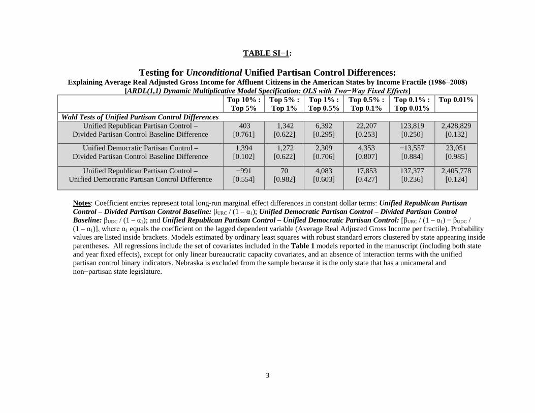
3
TABLE SI−1:
Testing for Unconditional Unified Partisan Control Differences: Explaining Average Real Adjusted Gross Income for Affluent Citizens in the American States by Income Fractile (1986−2008)
[ARDL(1,1) Dynamic Multiplicative Model Specification: OLS with Two−Way Fixed Effects] Top 10% :
Top 5% Top 5% : Top 1%
Top 1% : Top 0.5%
Top 0.5% : Top 0.1%
Top 0.1% : Top 0.01%
Top 0.01%
Wald Tests of Unified Partisan Control Differences Unified Republican Partisan Control –
Divided Partisan Control Baseline Difference 403
[0.761] 1,342 [0.622]
6,392 [0.295]
22,207 [0.253]
123,819 [0.250]
2,428,829 [0.132]
Unified Democratic Partisan Control – Divided Partisan Control Baseline Difference
1,394 [0.102]
1,272 [0.622]
2,309 [0.706]
4,353 [0.807]
−13,557 [0.884]
23,051 [0.985]
Unified Republican Partisan Control – Unified Democratic Partisan Control Difference
−991 [0.554]
70 [0.982]
4,083 [0.603]
17,853 [0.427]
137,377 [0.236]
2,405,778 [0.124]
Notes: Coefficient entries represent total long-run marginal effect differences in constant dollar terms: Unified Republican Partisan Control – Divided Partisan Control Baseline: βURC / (1 – α1); Unified Democratic Partisan Control – Divided Partisan Control Baseline: βUDC / (1 – α1); and Unified Republican Partisan Control – Unified Democratic Partisan Control: [βURC / (1 – α1) − βUDC / (1 – α1)], where α1 equals the coefficient on the lagged dependent variable (Average Real Adjusted Gross Income per fractile). Probability values are listed inside brackets. Models estimated by ordinary least squares with robust standard errors clustered by state appearing inside parentheses. All regressions include the set of covariates included in the Table 1 models reported in the manuscript (including both state and year fixed effects), except for only linear bureaucratic capacity covariates, and an absence of interaction terms with the unified partisan control binary indicators. Nebraska is excluded from the sample because it is the only state that has a unicameral and non−partisan state legislature.
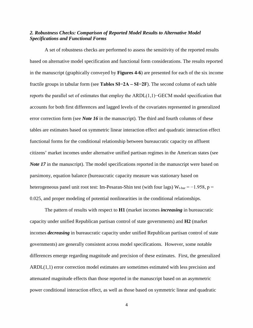
4
2. Robustness Checks: Comparison of Reported Model Results to Alternative Model Specifications and Functional Forms
A set of robustness checks are performed to assess the sensitivity of the reported results
based on alternative model specification and functional form considerations. The results reported
in the manuscript (graphically conveyed by Figures 4-6) are presented for each of the six income
fractile groups in tabular form (see Tables SI−2A – SI−2F). The second column of each table
reports the parallel set of estimates that employ the ARDL(1,1)−GECM model specification that
accounts for both first differences and lagged levels of the covariates represented in generalized
error correction form (see Note 16 in the manuscript). The third and fourth columns of these
tables are estimates based on symmetric linear interaction effect and quadratic interaction effect
functional forms for the conditional relationship between bureaucratic capacity on affluent
citizens’ market incomes under alternative unified partisan regimes in the American states (see
Note 17 in the manuscript). The model specifications reported in the manuscript were based on
parsimony, equation balance (bureaucratic capacity measure was stationary based on
heterogeneous panel unit root test: Im-Pesaran-Shin test (with four lags) Wt-bar = −1.958, p =
0.025, and proper modeling of potential nonlinearities in the conditional relationships.
The pattern of results with respect to H1 (market incomes increasing in bureaucratic
capacity under unified Republican partisan control of state governments) and H2 (market
incomes decreasing in bureaucratic capacity under unified Republican partisan control of state
governments) are generally consistent across model specifications. However, some notable
differences emerge regarding magnitude and precision of these estimates. First, the generalized
ARDL(1,1) error correction model estimates are sometimes estimated with less precision and
attenuated magnitude effects than those reported in the manuscript based on an asymmetric
power conditional interaction effect, as well as those based on symmetric linear and quadratic
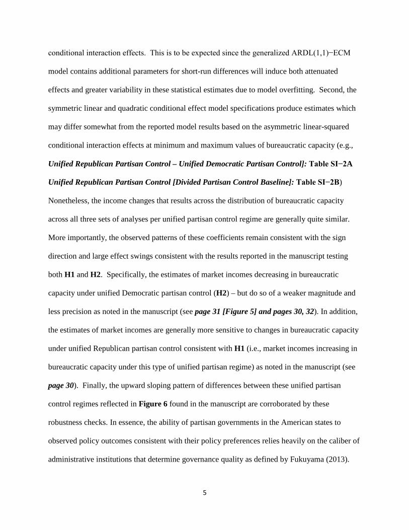
5
conditional interaction effects. This is to be expected since the generalized ARDL(1,1)−ECM
model contains additional parameters for short-run differences will induce both attenuated
effects and greater variability in these statistical estimates due to model overfitting. Second, the
symmetric linear and quadratic conditional effect model specifications produce estimates which
may differ somewhat from the reported model results based on the asymmetric linear-squared
conditional interaction effects at minimum and maximum values of bureaucratic capacity (e.g.,
Unified Republican Partisan Control – Unified Democratic Partisan Control]: Table SI−2A
Unified Republican Partisan Control [Divided Partisan Control Baseline]: Table SI−2B)
Nonetheless, the income changes that results across the distribution of bureaucratic capacity
across all three sets of analyses per unified partisan control regime are generally quite similar.
More importantly, the observed patterns of these coefficients remain consistent with the sign
direction and large effect swings consistent with the results reported in the manuscript testing
both H1 and H2. Specifically, the estimates of market incomes decreasing in bureaucratic
capacity under unified Democratic partisan control (H2) – but do so of a weaker magnitude and
less precision as noted in the manuscript (see page 31 [Figure 5] and pages 30, 32). In addition,
the estimates of market incomes are generally more sensitive to changes in bureaucratic capacity
under unified Republican partisan control consistent with H1 (i.e., market incomes increasing in
bureaucratic capacity under this type of unified partisan regime) as noted in the manuscript (see
page 30). Finally, the upward sloping pattern of differences between these unified partisan
control regimes reflected in Figure 6 found in the manuscript are corroborated by these
robustness checks. In essence, the ability of partisan governments in the American states to
observed policy outcomes consistent with their policy preferences relies heavily on the caliber of
administrative institutions that determine governance quality as defined by Fukuyama (2013).

6
TABLE SI-2A: Comparing Manuscript Reported Results Based on ARDL(1,1) Model Specification with Asymmetric Functional Form for Unified Partisan Control Interaction Effects
to Alternative Model Specifications and Functional Forms (Top 0.01% Income Fractile in Each State Per Year)
Hypothesis Test Reported Results
ARDL(1,1)-GECM
Symmetric Linear
Interaction Effects
Symmetric Quadratic Interaction
Effects
Unified Republican Partisan Control (Divided Partisan Control Baseline)
Minimum Value 2,550,280 [0.479]
2,796,033 [0.531]
−4,062,138 [0.207]
3,170,888 [0.402]
10th Percentile Value 367,223 [0.870]
784,762 [0.788]
−2,489,731 [0.281]
708,589 [0.760]
25th Percentile Value −862,911 [−0.505]
−422,297 [0.812]
−738,096 [0.600]
−761,780 [0.555]
50th Percentile Value −577,554 [0.525]
−369,569 [0,769]
1,523,990 [0.161]
−676,207 [0.456]
75th Percentile Value 2,499.517* [0.073]
2,048,065 [0.157]
4,207,103* [0.069]
2,325,317* [0.086]
90th Percentile Value 7,203,410*** [0.008]
5,907,042*** [0.04]
6,393,121* [0.075]
7,097,155*** [0.006]
Maximum Value 24,700,000*** [0.005]
20,600,000*** [0.001]
11,300,000* [0.086]
25,200,000***
[0.004]
Unified Democratic Partisan Control (Divided Partisan Control Baseline)
Reported Results
ARDL(1,1)-GECM
Symmetric Linear
Interaction Effects
Symmetric Quadratic Interaction
Effects
Minimum Value 2,785,887 [0.270]
937,121 [0.690]
2,347,597 [0.363]
5,544,772 [0.190]
10th Percentile Value 1,646,869 [0.289]
556,681 [0.771]
1,398,335 [0.374]
2,273,758 [0.213]
25th Percentile Value 1,004,109 [0.392]
341,996 [0.763]
862,661 [0.465]
874,836 [0.463]
50th Percentile Value 12,998 [0.991]
10,954 [0.991]
36,656 [0.977]
−650,332 [0.646]
75th Percentile Value −726,494 [0.671]
−232,693 [0.863]
−571,285 [0.744]
−1,283,050 [0.483]
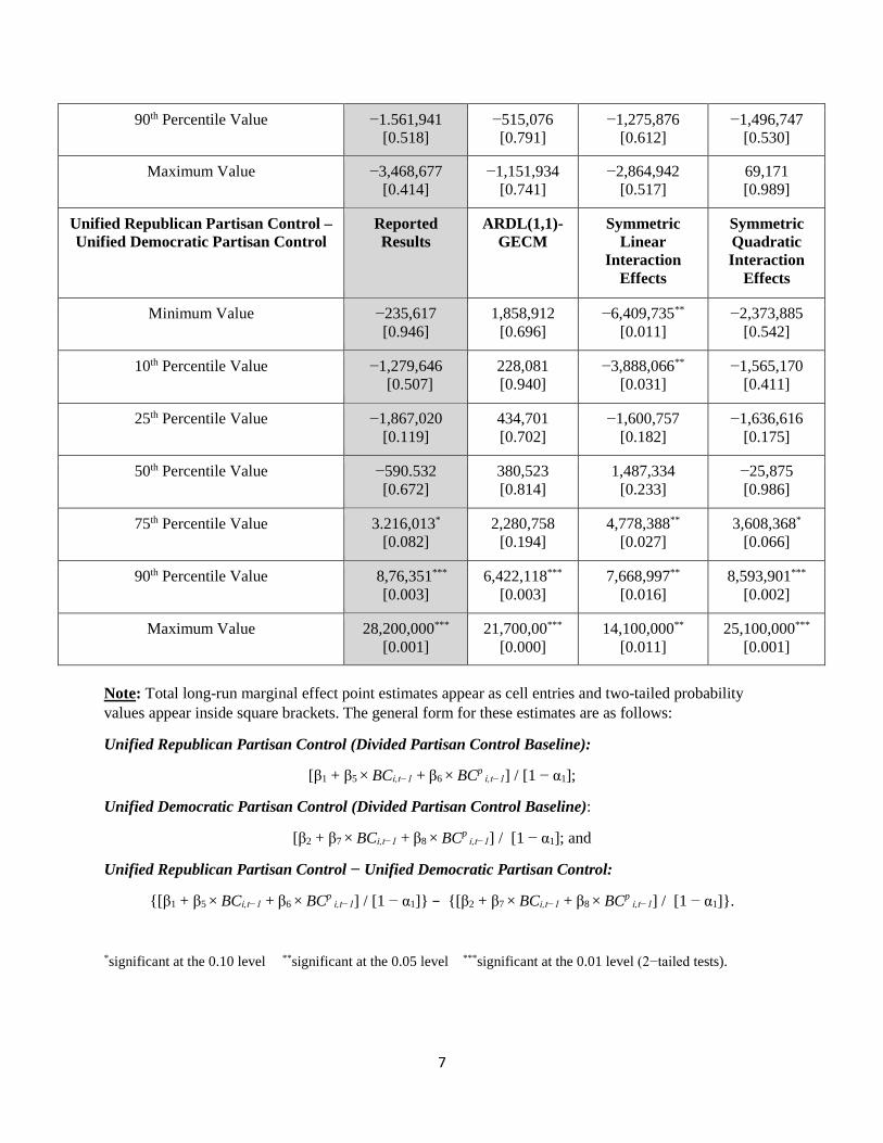
7
90th Percentile Value −1.561,941 [0.518]
−515,076 [0.791]
−1,275,876 [0.612]
−1,496,747 [0.530]
Maximum Value −3,468,677 [0.414]
−1,151,934 [0.741]
−2,864,942 [0.517]
69,171 [0.989]
Unified Republican Partisan Control – Unified Democratic Partisan Control
Reported Results
ARDL(1,1)-GECM
Symmetric Linear
Interaction Effects
Symmetric Quadratic Interaction
Effects
Minimum Value −235,617 [0.946]
1,858,912 [0.696]
−6,409,735**
[0.011] −2,373,885
[0.542]
10th Percentile Value −1,279,646 [0.507]
228,081 [0.940]
−3,888,066**
[0.031] −1,565,170
[0.411]
25th Percentile Value −1,867,020 [0.119]
434,701 [0.702]
−1,600,757 [0.182]
−1,636,616 [0.175]
50th Percentile Value −590.532 [0.672]
380,523 [0.814]
1,487,334 [0.233]
−25,875 [0.986]
75th Percentile Value 3.216,013* [0.082]
2,280,758 [0.194]
4,778,388** [0.027]
3,608,368* [0.066]
90th Percentile Value 8,76,351*** [0.003]
6,422,118*** [0.003]
7,668,997** [0.016]
8,593,901*** [0.002]
Maximum Value 28,200,000*** [0.001]
21,700,00*** [0.000]
14,100,000** [0.011]
25,100,000*** [0.001]
Note: Total long-run marginal effect point estimates appear as cell entries and two-tailed probability values appear inside square brackets. The general form for these estimates are as follows:
Unified Republican Partisan Control (Divided Partisan Control Baseline):
[β1 + β5 × BCi,t−1 + β6 × BCp i,t−1] / [1 − α1];
Unified Democratic Partisan Control (Divided Partisan Control Baseline):
[β2 + β7 × BCi,t−1 + β8 × BCp i,t−1] / [1 − α1]; and
Unified Republican Partisan Control − Unified Democratic Partisan Control:
{[β1 + β5 × BCi,t−1 + β6 × BCp i,t−1] / [1 − α1]} − {[β2 + β7 × BCi,t−1 + β8 × BCp
i,t−1] / [1 − α1]}.
*significant at the 0.10 level **significant at the 0.05 level ***significant at the 0.01 level (2−tailed tests).
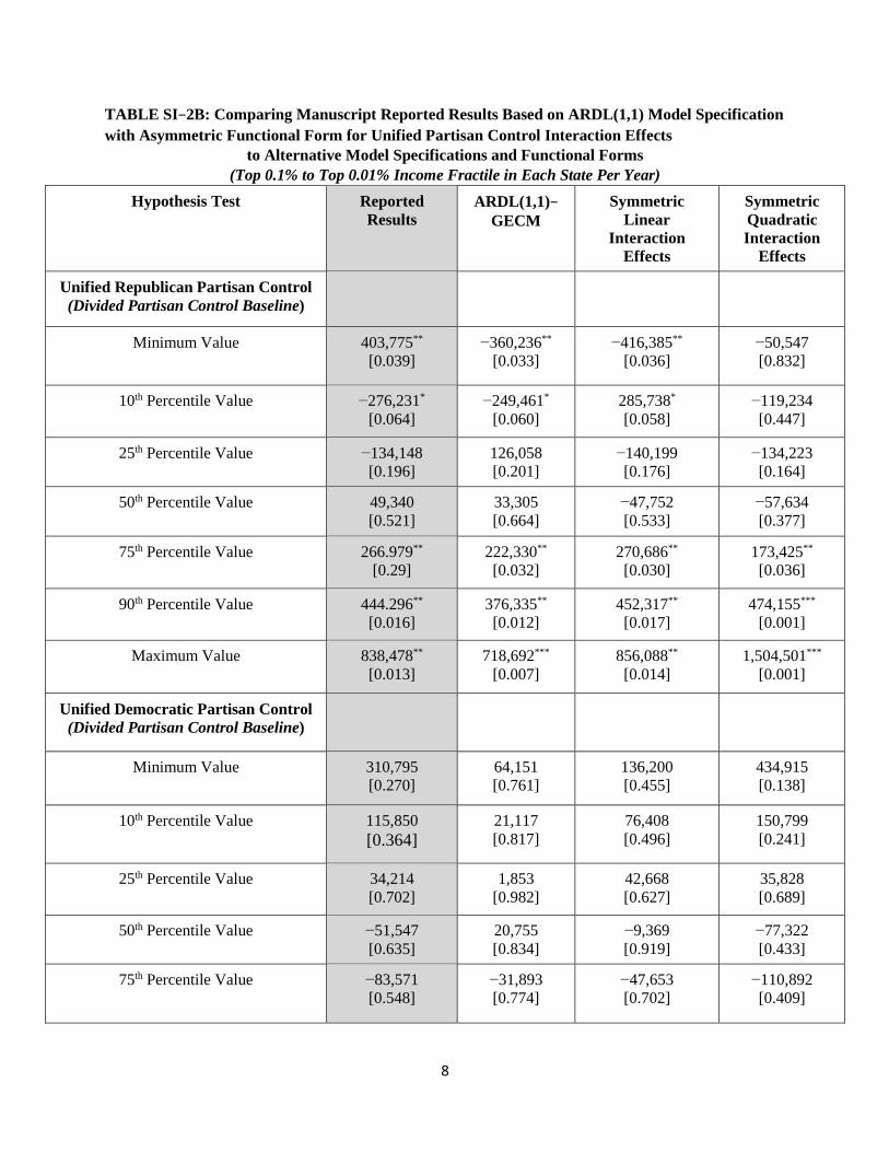
8
TABLE SI−2B: Comparing Manuscript Reported Results Based on ARDL(1,1) Model Specification with Asymmetric Functional Form for Unified Partisan Control Interaction Effects
to Alternative Model Specifications and Functional Forms (Top 0.1% to Top 0.01% Income Fractile in Each State Per Year)
Hypothesis Test Reported Results
ARDL(1,1)− GECM
Symmetric Linear
Interaction Effects
Symmetric Quadratic Interaction
Effects
Unified Republican Partisan Control (Divided Partisan Control Baseline)
Minimum Value 403,775** [0.039]
−360,236**
[0.033] −416,385**
[0.036] −50,547 [0.832]
10th Percentile Value −276,231* [0.064]
−249,461* [0.060]
285,738* [0.058]
−119,234 [0.447]
25th Percentile Value −134,148 [0.196]
126,058 [0.201]
−140,199 [0.176]
−134,223 [0.164]
50th Percentile Value 49,340 [0.521]
33,305 [0.664]
−47,752 [0.533]
−57,634 [0.377]
75th Percentile Value 266.979**
[0.29] 222,330** [0.032]
270,686** [0.030]
173,425** [0.036]
90th Percentile Value 444.296** [0.016]
376,335**
[0.012] 452,317** [0.017]
474,155***
[0.001]
Maximum Value 838,478** [0.013]
718,692***
[0.007] 856,088** [0.014]
1,504,501***
[0.001]
Unified Democratic Partisan Control (Divided Partisan Control Baseline)
Minimum Value 310,795 [0.270]
64,151 [0.761]
136,200 [0.455]
434,915 [0.138]
10th Percentile Value 115,850 [0.364]
21,117 [0.817]
76,408 [0.496]
150,799 [0.241]
25th Percentile Value 34,214 [0.702]
1,853 [0.982]
42,668 [0.627]
35,828 [0.689]
50th Percentile Value −51,547 [0.635]
20,755 [0.834]
−9,369 [0.919]
−77,322 [0.433]
75th Percentile Value −83,571 [0.548]
−31,893 [0.774]
−47,653 [0.702]
−110,892 [0.409]
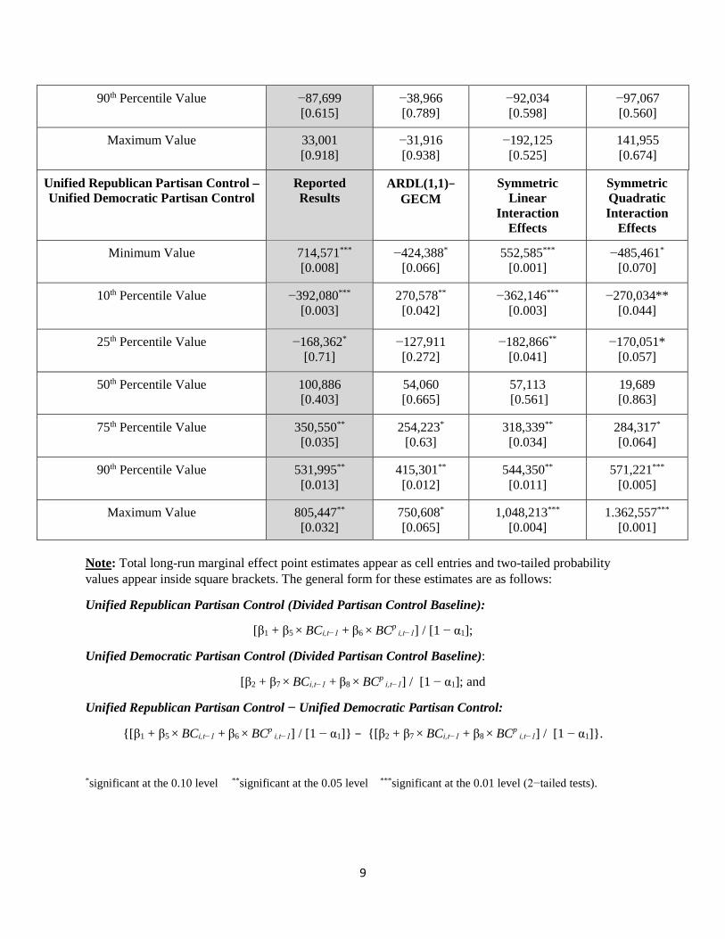
9
90th Percentile Value −87,699 [0.615]
−38,966 [0.789]
−92,034 [0.598]
−97,067 [0.560]
Maximum Value 33,001 [0.918]
−31,916 [0.938]
−192,125 [0.525]
141,955 [0.674]
Unified Republican Partisan Control – Unified Democratic Partisan Control
Reported Results
ARDL(1,1)− GECM
Symmetric Linear
Interaction Effects
Symmetric Quadratic Interaction
Effects
Minimum Value 714,571***
[0.008] −424,388*
[0.066] 552,585***
[0.001] −485,461*
[0.070]
10th Percentile Value −392,080***
[0.003] 270,578** [0.042]
−362,146*** [0.003]
−270,034** [0.044]
25th Percentile Value −168,362* [0.71]
−127,911 [0.272]
−182,866**
[0.041] −170,051*
[0.057]
50th Percentile Value 100,886 [0.403]
54,060 [0.665]
57,113 [0.561]
19,689 [0.863]
75th Percentile Value 350,550** [0.035]
254,223* [0.63]
318,339** [0.034]
284,317* [0.064]
90th Percentile Value 531,995** [0.013]
415,301** [0.012]
544,350** [0.011]
571,221***
[0.005]
Maximum Value 805,447** [0.032]
750,608* [0.065]
1,048,213*** [0.004]
1.362,557*** [0.001]
Note: Total long-run marginal effect point estimates appear as cell entries and two-tailed probability values appear inside square brackets. The general form for these estimates are as follows:
Unified Republican Partisan Control (Divided Partisan Control Baseline):
[β1 + β5 × BCi,t−1 + β6 × BCp i,t−1] / [1 − α1];
Unified Democratic Partisan Control (Divided Partisan Control Baseline):
[β2 + β7 × BCi,t−1 + β8 × BCp i,t−1] / [1 − α1]; and
Unified Republican Partisan Control − Unified Democratic Partisan Control:
{[β1 + β5 × BCi,t−1 + β6 × BCp i,t−1] / [1 − α1]} − {[β2 + β7 × BCi,t−1 + β8 × BCp
i,t−1] / [1 − α1]}.
*significant at the 0.10 level **significant at the 0.05 level ***significant at the 0.01 level (2−tailed tests).

10
TABLE SI−2C: Comparing Manuscript Reported Results Based on ARDL(1,1) Model Specification with Asymmetric Functional Form for Unified Partisan Control Interaction Effects
to Alternative Model Specifications and Functional Forms (Top 0.5% to Top 0.1% Income Fractile in Each State Per Year)
Hypothesis Test Reported Results ARDL(1,1)− GECM
Symmetric Linear
Interaction Effects
Symmetric Quadratic Interaction
Effects
Unified Republican Partisan Control (Divided Partisan Control Baseline)
Minimum Value −78,729*** [0.009]
−64,258** [0.024]
−83,717***
[0.07] −34,255 [0.340]
10th Percentile Value −54,298** [0.019]
−44,582** [0.048]
−58,065** [0.014]
-34,515 [0.137]
25th Percentile Value −27.081* [0.098]
−22,663 [0.181]
−29,489* [0.075]
−27,063* [0.076]
50th Percentile Value 8,067 [0.543]
5,643 [0.675]
7,414 [0.577]
−5,369 [0.694]
75th Percentile Value 49,757** [0.017]
39,219** [0.029]
51,186**
[0.017] 38,004** [0.028]
90th Percentile Value 83,722**
[0.006] 66,573*** [0.009]
86,849*** [0.006]
87,493*** [0.001]
Maximum Value 159,230***
[0.004] 127,384***
[0.005] 166,128***
[0.004] 243,029***
[0.001]
Unified Democratic Partisan Control (Divided Partisan Control Baseline)
Reported Results ARDL(1,1)− GECM
Symmetric Linear
Interaction Effects
Symmetric Quadratic Interaction
Effects
Minimum Value 102,758* [0.086]
52,626 [0.197]
36,593 [0.280]
118,143** [0.048]
10th Percentile Value 38,316 [0.127]
15,987 [0.399]
23,466 [0.259]
42,608* [0.088]
25th Percentile Value 12,728 [0.455]
2,299 [0.890]
16,058 [0.320]
12,883 [0.452]
50th Percentile Value −11,453 [0.601]
−8,926 [0.651]
4,635 [0.797]
−14,711 [0.498]
75th Percentile Value −17,436 [0.527]
−9,528 [0.666]
−3,773 [0.880]
−20,883 [0.438]

11
90th Percentile Value −11,831 [0.728]
−2,103 [0.937]
−13,517 [0.702]
−13,038 [0.692]
Maximum Value 50.234 [0.464]
46,666 [0.472]
−35,493 [0.560]
63,764 [0.362]
Unified Republican Partisan Control – Unified Democratic Partisan Control
Reported Results ARDL(1,1)− GECM
Symmetric Linear
Interaction Effects
Symmetric Quadratic Interaction
Effects
Minimum Value −181,487***
[0.002] −116,885**
[0.020] −120,311***
[0.000] −152,397**
[0.014]
10th Percentile Value −92,614***
[0.000] 60,569** [0.035]
−81,531***
[0.000] −77,122***
[0.003]
25th Percentile Value −39,819**
[0.011] −24,962 [0.279]
−45,547*** [0.002]
−39,946*** [0.009]
50th Percentile Value 19,520 [0.412]
14,569 [0.532]
2,779 [0.884]
9,343 [0.702]
75th Percentile Value 67,193** [0.046]
48,747* [0.061]
54,959* [0.070]
58,887* [0.007]
90th Percentile Value 95,553** [0.026]
68,676** [0.022]
100,366** [0.021]
100,531**
[0.015]
Maximum Value 108,996 [0.162]
80,718 [0.195]
201,620***
[0.007] 179,265** [0.036]
Note: Total long-run marginal effect point estimates appear as cell entries and two-tailed probability values appear inside square brackets. The general form for these estimates are as follows:
Unified Republican Partisan Control (Divided Partisan Control Baseline):
[β1 + β5 × BCi,t−1 + β6 × BCp i,t−1] / [1 − α1];
Unified Democratic Partisan Control (Divided Partisan Control Baseline):
[β2 + β7 × BCi,t−1 + β8 × BCp i,t−1] / [1 − α1]; and
Unified Republican Partisan Control − Unified Democratic Partisan Control:
{[β1 + β5 × BCi,t−1 + β6 × BCp i,t−1] / [1 − α1]} − {[β2 + β7 × BCi,t−1 + β8 × BCp
i,t−1] / [1 − α1]}.
*significant at the 0.10 level **significant at the 0.05 level ***significant at the 0.01 level (2−tailed tests).
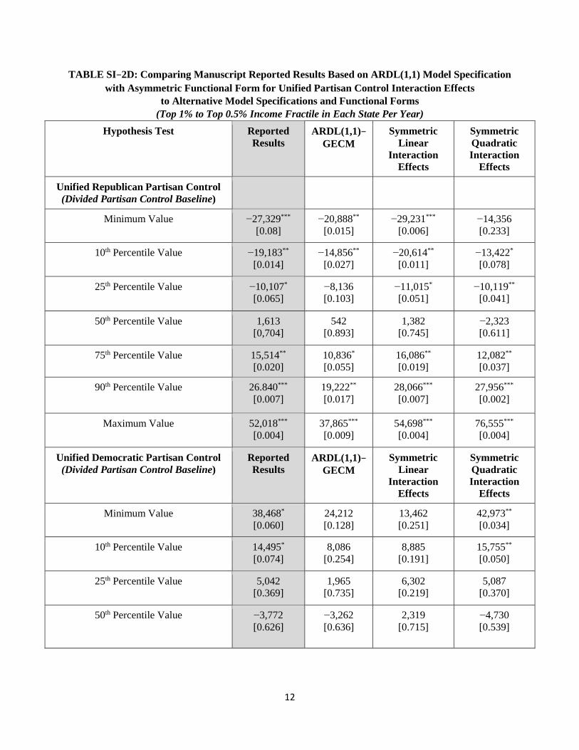
12
TABLE SI−2D: Comparing Manuscript Reported Results Based on ARDL(1,1) Model Specification with Asymmetric Functional Form for Unified Partisan Control Interaction Effects
to Alternative Model Specifications and Functional Forms (Top 1% to Top 0.5% Income Fractile in Each State Per Year)
Hypothesis Test Reported Results
ARDL(1,1)−GECM
Symmetric Linear
Interaction Effects
Symmetric Quadratic Interaction
Effects
Unified Republican Partisan Control (Divided Partisan Control Baseline)
Minimum Value −27,329*** [0.08]
−20,888** [0.015]
−29,231***
[0.006] −14,356 [0.233]
10th Percentile Value −19,183** [0.014]
−14,856** [0.027]
−20,614** [0.011]
−13,422* [0.078]
25th Percentile Value −10,107* [0.065]
−8,136 [0.103]
−11,015* [0.051]
−10,119** [0.041]
50th Percentile Value 1,613 [0,704]
542 [0.893]
1,382 [0.745]
−2,323 [0.611]
75th Percentile Value 15,514**
[0.020] 10,836* [0.055]
16,086** [0.019]
12,082** [0.037]
90th Percentile Value 26.840*** [0.007]
19,222** [0.017]
28,066*** [0.007]
27,956***
[0.002]
Maximum Value 52,018***
[0.004] 37,865*** [0.009]
54,698***
[0.004] 76,555***
[0.004]
Unified Democratic Partisan Control (Divided Partisan Control Baseline)
Reported Results
ARDL(1,1)−GECM
Symmetric Linear
Interaction Effects
Symmetric Quadratic Interaction
Effects
Minimum Value 38,468* [0.060]
24,212 [0.128]
13,462 [0.251]
42,973** [0.034]
10th Percentile Value 14,495* [0.074]
8,086 [0.254]
8,885 [0.191]
15,755**
[0.050]
25th Percentile Value 5,042 [0.369]
1,965 [0.735]
6,302 [0.219]
5,087 [0.370]
50th Percentile Value −3,772 [0.626]
−3,262 [0.636]
2,319 [0.715]
−4,730 [0.539]
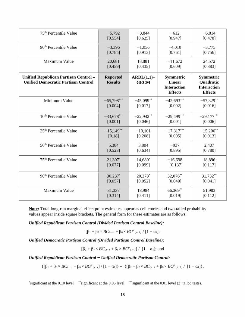
13
75th Percentile Value −5,792 [0.554]
−3,844 [0.625]
−612 [0.947]
−6,814 [0.478]
90th Percentile Value −3,396 [0.785]
−1,056 [0.913]
−4,010 [0.761]
−3,775 [0.756]
Maximum Value 20,681 [0.459]
18,881 [0.435]
−11,672 [0.609]
24,572 [0.383]
Unified Republican Partisan Control – Unified Democratic Partisan Control
Reported Results
ARDL(1,1)−GECM
Symmetric Linear
Interaction Effects
Symmetric Quadratic Interaction
Effects
Minimum Value −65,798***
[0.004] −45,099**
[0.017] −42,693***
[0.002] −57,329**
[0.016]
10th Percentile Value −33,678***
[0.001] −22,942**
[0.046] −29,499***
[0.001] −29,177***
[0.006]
25th Percentile Value −15,149** [0.18]
−10,101 [0.208]
−17,317*** [0.005]
−15,206** [0.013]
50th Percentile Value 5,384 [0.523]
3,804 [0.634]
−937 [0.895]
2,407 [0.780]
75th Percentile Value 21,307* [0.077]
14,680* [0.099]
−16,698 [0.137]
18,896 [0.117]
90th Percentile Value 30,237* [0.057]
20,278* [0.052]
32,076** [0.049]
31,732**
[0.041]
Maximum Value 31,337 [0.314]
18,984 [0.411]
66,369** [0.019]
51,983 [0.112]
Note: Total long-run marginal effect point estimates appear as cell entries and two-tailed probability values appear inside square brackets. The general form for these estimates are as follows:
Unified Republican Partisan Control (Divided Partisan Control Baseline):
[β1 + β5 × BCi,t−1 + β6 × BCp i,t−1] / [1 − α1];
Unified Democratic Partisan Control (Divided Partisan Control Baseline):
[β2 + β7 × BCi,t−1 + β8 × BCp i,t−1] / [1 − α1]; and
Unified Republican Partisan Control − Unified Democratic Partisan Control:
{[β1 + β5 × BCi,t−1 + β6 × BCp i,t−1] / [1 − α1]} − {[β2 + β7 × BCi,t−1 + β8 × BCp
i,t−1] / [1 − α1]}.
*significant at the 0.10 level **significant at the 0.05 level ***significant at the 0.01 level (2−tailed tests).
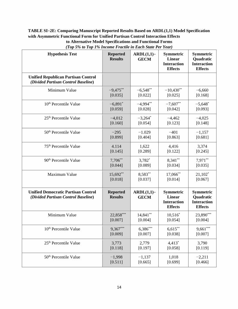
14
TABLE SI−2E: Comparing Manuscript Reported Results Based on ARDL(1,1) Model Specification with Asymmetric Functional Form for Unified Partisan Control Interaction Effects
to Alternative Model Specifications and Functional Forms (Top 5% to Top 1% Income Fractile in Each State Per Year)
Hypothesis Test Reported Results
ARDL(1,1)−GECM
Symmetric Linear
Interaction Effects
Symmetric Quadratic Interaction
Effects
Unified Republican Partisan Control (Divided Partisan Control Baseline)
Minimum Value −9,475** [0.035]
−6,548** [0.022]
−10,430** [0.025]
−6,660 [0.168]
10th Percentile Value −6,891* [0.059]
−4,994** [0.028]
−7,607** [0.042]
−5,648* [0.093]
25th Percentile Value −4,012 [0.160]
−3,264* [0.054]
−4,462 [0.123]
−4,025 [0.148]
50th Percentile Value −295 [0.899]
−1.029 [0.404]
−401 [0.863]
−1,157 [0.681]
75th Percentile Value 4.114 [0.145]
1,622 [0.289]
4,416 [0.122]
3,374 [0.245]
90th Percentile Value 7,706**
[0.044] 3,782* [0.089]
8,341** [0.034]
7,971**
[0.035]
Maximum Value 15,692**
[0.018] 8,583** [0.037]
17,066** [0.014]
21,102* [0.067]
Unified Democratic Partisan Control (Divided Partisan Control Baseline)
Reported Results
ARDL(1,1)−GECM
Symmetric Linear
Interaction Effects
Symmetric Quadratic Interaction
Effects
Minimum Value 22,858*** [0.007]
14,841** [0.004]
10,516* [0.054]
23,890*** [0.004]
10th Percentile Value 9,367*** [0.009]
6,386***
[0.007] 6,615** [0.038]
9,661*** [0.007]
25th Percentile Value 3,773 [0.118]
2,779 [0.197]
4,413* [0.058]
3,790 [0.119]
50th Percentile Value −1,998 [0.511]
−1,137 [0.665]
1,018 [0.699]
−2,211 [0.466]

15
75th Percentile Value −4,032 [0.312]
−2,745 [0.349]
−1,481 [0.701]
−4,63 [0.280]
90th Percentile Value −4,041 [0.447]
−3,255 [0.357]
−4,377 [0.435]
−4,123 [0.433]
Maximum Value 5,191 [0.661]
927 [0.916]
−10,908 [0.269]
6,053 [0.615]
Unified Republican Partisan Control – Unified Democratic Partisan Control
Reported Results
ARDL(1,1)−GECM
Symmetric Linear
Interaction Effects
Symmetric Quadratic Interaction
Effects
Minimum Value −32,333*** [0.001]
−21,388*** [0.000]
−20,946*** [0.002]
−30,550*** [0.003]
10th Percentile Value −26,257***
[0.002] −11,381***
[0.001] −14,222***
[0.002] −15,309***
[0.003]
25th Percentile Value −7,785** [0.030]
−6,043** [0.023]
−8,875*** [0.010]
−7,815**
[0.027]
50th Percentile Value 1,703 [0.640]
109 [0.969]
−1,419 [0.662]
1,055 [0.789]
75th Percentile Value 8,146* [0.091]
4,367 [0.143]
5,897 [0.191]
7,637 [0.123]
90th Percentile Value 11,747* [0.069]
7,037** [0.048]
12,718* [0.052]
12,103* [0.060]
Maximum Value 10,501 [0.418]
7,657 [0.387]
27,974** [0.016]
15,049 [0.299]
Note: Total long-run marginal effect point estimates appear as cell entries and two-tailed probability values appear inside square brackets. The general form for these estimates are as follows:
Unified Republican Partisan Control (Divided Partisan Control Baseline):
[β1 + β5 × BCi,t−1 + β6 × BCp i,t−1] / [1 − α1];
Unified Democratic Partisan Control (Divided Partisan Control Baseline):
[β2 + β7 × BCi,t−1 + β8 × BCp i,t−1] / [1 − α1]; and
Unified Republican Partisan Control − Unified Democratic Partisan Control:
{[β1 + β5 × BCi,t−1 + β6 × BCp i,t−1] / [1 − α1]} − {[β2 + β7 × BCi,t−1 + β8 × BCp
i,t−1] / [1 − α1]}.
*significant at the 0.10 level **significant at the 0.05 level ***significant at the 0.01 level (2−tailed tests).
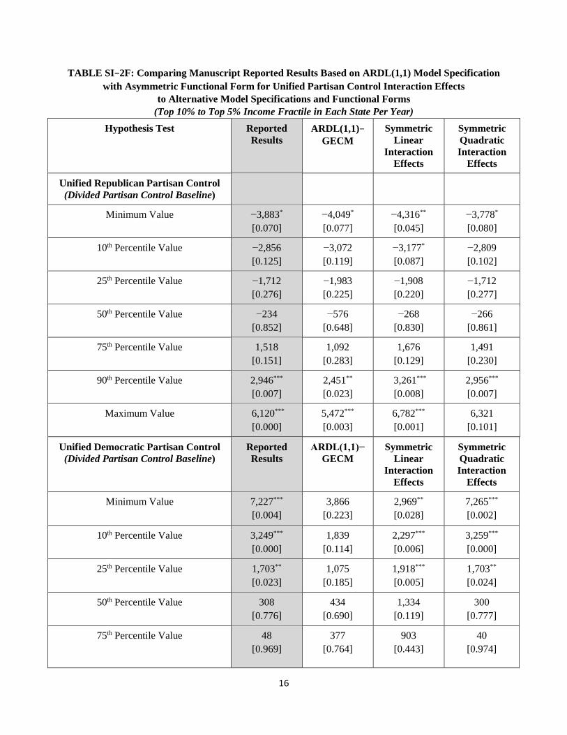
16
TABLE SI−2F: Comparing Manuscript Reported Results Based on ARDL(1,1) Model Specification with Asymmetric Functional Form for Unified Partisan Control Interaction Effects
to Alternative Model Specifications and Functional Forms (Top 10% to Top 5% Income Fractile in Each State Per Year)
Hypothesis Test Reported Results
ARDL(1,1)− GECM
Symmetric Linear
Interaction Effects
Symmetric Quadratic Interaction
Effects
Unified Republican Partisan Control (Divided Partisan Control Baseline)
Minimum Value −3,883* [0.070]
−4,049* [0.077]
−4,316** [0.045]
−3,778* [0.080]
10th Percentile Value −2,856 [0.125]
−3,072 [0.119]
−3,177* [0.087]
−2,809 [0.102]
25th Percentile Value −1,712 [0.276]
−1,983 [0.225]
−1,908 [0.220]
−1,712 [0.277]
50th Percentile Value −234 [0.852]
−576 [0.648]
−268 [0.830]
−266 [0.861]
75th Percentile Value 1,518 [0.151]
1,092 [0.283]
1,676 [0.129]
1,491 [0.230]
90th Percentile Value 2,946*** [0.007]
2,451** [0.023]
3,261*** [0.008]
2,956*** [0.007]
Maximum Value 6,120*** [0.000]
5,472*** [0.003]
6,782*** [0.001]
6,321 [0.101]
Unified Democratic Partisan Control (Divided Partisan Control Baseline)
Reported Results
ARDL(1,1)− GECM
Symmetric Linear
Interaction Effects
Symmetric Quadratic Interaction
Effects
Minimum Value 7,227*** [0.004]
3,866 [0.223]
2,969**
[0.028] 7,265*** [0.002]
10th Percentile Value 3,249***
[0.000] 1,839
[0.114] 2,297*** [0.006]
3,259*** [0.000]
25th Percentile Value 1,703** [0.023]
1,075 [0.185]
1,918***
[0.005] 1,703** [0.024]
50th Percentile Value 308 [0.776]
434 [0.690]
1,334 [0.119]
300 [0.777]
75th Percentile Value 48 [0.969]
377 [0.764]
903 [0.443]
40 [0.974]
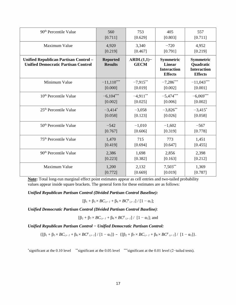
17
90th Percentile Value 560 [0.711]
753 [0.629]
405 [0.803]
557 [0.711]
Maximum Value 4,920 [0.219]
3,340 [0.467]
−720 [0.791]
4,952 [0.219]
Unified Republican Partisan Control – Unified Democratic Partisan Control
Reported Results
ARDL(1,1)− GECM
Symmetric Linear
Interaction Effects
Symmetric Quadratic Interaction
Effects
Minimum Value −11,110*** [0.000]
−7,915** [0.019]
−7,286*** [0.002]
−11,043*** [0.001]
10th Percentile Value −6,104*** [0.002]
−4,911** [0.025]
−5,474*** [0.006]
−6,069*** [0.002]
25th Percentile Value −3,414*
[0.058] −3,058 [0.123]
−3,826**
[0.026] −3,415* [0.058]
50th Percentile Value −542 [0.767]
−1,010 [0.606]
−1,602 [0.319]
−567 [0.778]
75th Percentile Value 1,470 [0.419]
715 [0.694]
773 [0.647]
1,451 [0.455]
90th Percentile Value 2,386 [0.223]
1,698 [0.382]
2,856 [0.163]
2,398 [0.212]
Maximum Value 1,200 [0.772]
2,132 [0.669]
7,503** [0.019]
1,369 [0.787]
Note: Total long-run marginal effect point estimates appear as cell entries and two-tailed probability values appear inside square brackets. The general form for these estimates are as follows:
Unified Republican Partisan Control (Divided Partisan Control Baseline):
[β1 + β5 × BCi,t−1 + β6 × BCp i,t−1] / [1 − α1];
Unified Democratic Partisan Control (Divided Partisan Control Baseline):
[β2 + β7 × BCi,t−1 + β8 × BCp i,t−1] / [1 − α1]; and
Unified Republican Partisan Control − Unified Democratic Partisan Control:
{[β1 + β5 × BCi,t−1 + β6 × BCp i,t−1] / [1 − α1]} − {[β2 + β7 × BCi,t−1 + β8 × BCp
i,t−1] / [1 − α1]}.
*significant at the 0.10 level **significant at the 0.05 level ***significant at the 0.01 level (2−tailed tests).