Embed Size (px)
Citation preview

1
THE GLOBAL PRODUCTIVITY SLOWDOWN, TECHNOLOGY
DIVERGENCE AND PUBLIC POLICY: A FIRM LEVEL
PERSPECTIVE
Dan Andrews†, Chiara Criscuolo†† and Peter N. Gal†
† Economics Department, OECD
†† Directorate for Science, Technology and Innovation, OECD
2
ABSTRACT
The Global Productivity Slowdown, Technology Divergence and Public Policy: A Firm Level
Perspective
In this paper, we aim to bring the debate on the global productivity slowdown – which has largely been
conducted from a macroeconomic perspective – to a more micro-level. We show that a particularly
striking feature of the productivity slowdown is not so much a lower productivity growth at the global
frontier, but rather rising labour productivity at the global frontier coupled with an increasing labour
productivity divergence between the global frontier and laggard (non-frontier) firms. This productivity
divergence remains after controlling for differences in capital deepening and mark-up behaviour,
suggesting that divergence in measured multi-factor productivity (MFP) may in fact reflect
technological divergence in a broad sense. This divergence could plausibly reflect the potential for
structural changes in the global economy – namely digitalisation, globalisation and the rising importance
of tacit knowledge – to fuel rapid productivity gains at the global frontier. Yet, aggregate MFP
performance was significantly weaker in industries where MFP divergence was more pronounced,
suggesting that the divergence observed is not solely driven by frontier firms pushing the boundary
outward. We contend that increasing MFP divergence – and the global productivity slowdown more
generally – could reflect a slowdown in the diffusion process. This could be a reflection of increasing
costs for laggard firms of moving from an economy based on production to one based on ideas. But it
could also be symptomatic of rising entry barriers and a decline in the contestability of markets. We find
the rise in MFP divergence to be much more extreme in sectors where pro-competitive product market
reforms were least extensive, suggesting that policy weaknesses may be stifling diffusion in OECD
economies.
3
TABLE OF CONTENTS
THE GLOBAL PRODUCTIVITY SLOWDOWN, TECHNOLOGY DIVERGENCE AND PUBLIC
POLICY: A FIRM LEVEL PERSPECTIVE ............................................................................. 5 1. Introduction and main findings........................................................................................... 5 2. The productivity slowdown ................................................................................................ 7
2.1 Techno-pessimists and techno-optimists ................................................................... 8 2.2 Macroeconomic factors ............................................................................................. 9 2.3 Rising resource misallocation ................................................................................. 10 2.4 Measurement issues ................................................................................................. 10 2.5 Our contribution ...................................................................................................... 10
3. Data and identification of the global productivity frontier ............................................... 11 3.1 Productivity measurement ....................................................................................... 13 3.2 Correcting for mark-ups .......................................................................................... 13 3.3 Measuring the productivity frontier......................................................................... 15 3.4 Characteristics of frontier firms .............................................................................. 15
4. Productivity divergence between the global frontier and laggard firms ........................... 18 4.1 Labour productivity divergence .............................................................................. 18 4.2 Labour productivity divergence: capital deepening or MFP? ................................. 20 4.3 MFP divergence: mark-ups or technology? ............................................................ 22 4.4 MFP divergence: contributing factors ..................................................................... 24
5. Productivity divergence: aggregate implications and the role of policy .......................... 31 5.1 Aggregate implications ............................................................................................ 31 5.2 Productivity divergence and product market regulation.......................................... 32 5.3 Product market reforms in OECD countries ........................................................... 33 5.4 Empirical strategy.................................................................................................... 36 5.5 Empirical results ...................................................................................................... 38
6. Conclusion and future research ........................................................................................ 41
REFERENCES ............................................................................................................................ 43
APPENDIX A: DIVERGENCE INDICATORS......................................................................... 49
APPENDIX B: DIVERGENCE WITHIN MORE NARROWLY DEFINED INDUSTRIES ... 57
APPENDIX C: MFP CONVERGENCE AT THE FIRM LEVEL ............................................. 60
APPENDIX D: POLICY ANALYSIS – DESCRIPTIVES AND ROBUSTNESS .................... 62
APPENDIX E: DATA AND PRODUCTIVITY MEASUREMENT ......................................... 68
Tables
Table 1. Mean firm characteristics: frontier firms vs other firms...................................... 17 Table 2. MFP divergence and product market regulation in services ............................... 39 Table C1. The pace of productivity convergence has slowed over time .............................. 61 Table D1. Descriptive statistics by broad sectors ................................................................. 62 Table D2. Productivity divergence: link with aggregate productivity performance ................ 63 Table D3. MFP divergence and PMR in services: long difference window ........................ 64 Table D4. MFP divergence and PMR in services: median MFP of laggard firms ............... 65 Table D5. IV estimation: MFP divergence and product market regulations in services ...... 66 Table D6. MFP divergence in manufacturing and upstream product market regulation ..... 67 Table E1. Information providers underlying the Orbis Database ........................................ 68
4
Figures
Figure 1. Weak labour productivity underpinned the decline in potential output in OECD countries
8 Figure 2. A widening labour productivity gap between global frontier firms and other firms19 Figure 3. The widening labour productivity gap is mainly driven by MFP divergence ..... 21 Figure 4. The widening MFP gap remains after controlling for mark-ups ......................... 23 Figure 5. A widening gap in mark-up corrected MFP ........................................................ 24 Figure 6. Evidence on winner takes all dynamics ............................................................... 26 Figure 7. The pace of convergence slowed, even before the crisis ..................................... 28 Figure 8. Entry into the global frontier has become more entrenched amongst top quintile firms
29 Figure 9. Indicators of declining market dynamism amongst laggard firms ...................... 30 Figure 10. Aggregate MFP performance was weaker in industries where MFP divergence was
greater 32 Figure 11. The restrictiveness of product market regulations over time, 1998-2013 ....... 35 Figure 12. Slower product market reform, a larger increase in the MFP gap ................... 36 Figure 13. MFP divergence and market reforms in services ............................................ 40 Figure A1. Divergence: average industry level productivity ............................................. 49 Figure A2. Divergence: alternative labour productivity definition ................................... 50 Figure A3. Divergence: alternative frontier definitions ..................................................... 51 Figure A4. Divergence: excluding firms part of a MNE group ......................................... 52 Figure A5. Divergence: firm size indicators ...................................................................... 53 Figure A6. Divergence: alternative MFPR definitions ...................................................... 54 Figure A7. Divergence: by ICT intensity .......................................................................... 55 Figure A8. Divergence: mark-up corrected MFP using materials as flexible inputs ......... 56 Figure B1. Labour productivity divergence within more narrowly defined industries ..... 57 Figure B2. MFPR divergence within more narrowly defined industries .......................... 58 Figure B3. Mark-up corrected MFPR divergence within more narrowly defined industries59
5
THE GLOBAL PRODUCTIVITY SLOWDOWN, TECHNOLOGY DIVERGENCE AND
PUBLIC POLICY: A FIRM LEVEL PERSPECTIVE
Dan Andrews, Chiara Criscuolo and Peter N. Gal1
1. Introduction and main findings
1. Aggregate productivity growth slowed in many OECD countries, even before the crisis,
igniting a spirited debate on the future of productivity (e.g. Gordon, 2012 vs Brynjolfsson and McAfee,
2011).2 This paper marshals new firm level evidence to shed new light on the factors behind the global
slowdown in productivity growth – a debate which has by and large been conducted from a
macroeconomic perspective. While this debate often concerns the prospects for innovation at the global
productivity frontier, little is actually known about the productivity growth performance of global
frontier firms over time both in absolute terms and relative to laggard (i.e. non-frontier) firms.3 Even
less is known about the policies that might help laggard firms close their productivity growth gap with
the frontier. Yet, cross-country differences in aggregate-level productivity are increasingly being linked
to the widespread heterogeneity in firm performance within sectors (Bartelsman, Haltiwanger and
Scarpetta, 2013; Hsieh and Klenow, 2009).
2. To fill this gap, we highlight a number of policy-relevant issues related to the performance of
frontier firms and laggards, with a view to also shed light on recent aggregate productivity developments
in OECD countries. Using a harmonised cross-country firm-level database for 24 countries, we define
global frontier firms as the top 5% of firms in terms of labour productivity or multi-factor productivity
(MFP) levels within each two-digit sector in each year across all countries since the early 2000s. Our
analysis suggests that a striking feature of the productivity slowdown is not so much a slowing in
productivity growth at the global frontier, but rather rising productivity at the global frontier coupled
with an increasing productivity gap between the global frontier and laggard firms. In fact, slow
productivity growth of the “average” firm masks the fact that a small cadre of firms are experiencing
robust gains.
1 Corresponding authors are: Dan Andrews ([email protected]) and Peter Gal ([email protected]) from the
OECD Economics Department and Chiara Criscuolo ([email protected]) from the OECD Science,
Technology and Innovation Directorate. The authors would like to thank Martin Baily, Eric Bartelsman, Flora
Bellone, Giuseppe Berlingieri, Patrick Blanchenay, Erik Brynjolffson, Sarah Calligaris, Gilbert Cette, John Fernald,
Dominique Guellec, Jonathan Haskel, Nick Johnstone, Remy Lecat, Catherine L. Mann, Giuseppe Nicoletti, Dirk
Pilat, Xavier Ragot, Alessandro Saia, Jean-Luc Schneider, Louise Sheiner, John Van Reenen and Andrew Wyckoff
for their valuable comments. We would also like to thank seminar participants at the Bank of England, Central
Bank of the Netherlands, France Strategie, IMF, MIT, Peterson Institute for International Economics, UCL, US
Census Bureau, the OECD Global Forum on Productivity Conferences in Mexico City and Lisbon and OECD
Committee Meetings. The views expressed in this paper are those of the authors and do not necessarily reflect those
of the OECD or its member countries.
2 Some argue that the low-hanging fruit has already been picked: the IT revolution has run its course and other new
technologies like biotech have yet to make a major impact on our lives (Gordon, 2012). Others see the IT revolution
continuing apace, fuelling disruptive new business models and enabling a new wave of productivity growth across
the economy (Brynjolfsson and McAfee, 2011; Mokyr, 2014).
3 Throughout the paper we use the term “laggard” and “non-frontier” interchangeably – they refer to the group of
firms that are not at the frontier.
6
3. We show that the rising labour productivity gap between global frontier and laggard firms
largely reflects divergence in revenue based MFP (MFPR), as opposed to capital deepening. Moreover,
we explore the role of market power and conclude that divergence in MFPR does not simply reflect the
increasing ability of frontier firms to charge higher mark-ups. While there is evidence that market power
of frontier firms has increased in services, this amounts to less than one-third of the total divergence in
MFPR. This leads us to the conclusion that the rising MFPR gap between global frontier and laggard
firms may in fact reflect divergence in productivity or technology, broadly defined. Importantly, this is
likely to relate not only to the diverging capacity of firms to technologically innovate but also to their
success in tacitly combining various intangibles – e.g. computerised information; innovative property
and economic competencies (see Corrado, Hulten and Sichel, 2009) – in production processes.
4. This pattern of MFP divergence might seem surprising for at least two reasons. First, neo-
Schumpeterian growth theory (Aghion and Howitt, 2006; Acemoglu, Aghion and Zilibotti, 2006) and
models of competitive diffusion (Jovanovic and MacDonald, 1994) imply productivity convergence:
that is, firms further behind the global frontier should grow faster, given the larger stock of unexploited
technologies and knowledge that they can readily implement. Second, the extent of productivity
divergence that we observed in the data is difficult to reconcile with models of creative destruction and
a world where the process of market selection is productivity-enhancing (Aghion and Howitt, 1992;
Caballero and Hammour, 1994; Campbell, 1998), raising questions about the competitiveness of
markets. However, our results suggest that both the rate of convergence and growth-enhancing
reallocation have slowed down during the last decade leading to the divergence evident in the data.
5. The paper then explores a set of structural factors underlying MFP divergence, links with
aggregate productivity performance and public policy implications. Structural changes in the global
economy – namely digitalisation, globalisation and the rising importance of tacit knowledge – could
underpin MFP divergence through two interrelated channels introduced below. While it is difficult to
pinpoint their relative importance, a number of smoking guns emerge to suggest that each may be
important in explaining MFP divergence.
6. First, the increasing potential for digital technologies to unleash winner takes all dynamics in
the global market (Brynjolfsson and McAfee, 2011) has enabled technological leaders to increase their
performance gap with laggard firms. In support of this hypothesis, we find three distinct patterns in ICT-
intensive services (e.g. computer programming, telecommunications and information service activities )
– where winner take all patterns should be more relevant – that are less evident elsewhere: i) global
frontier firms have increased their market share; ii) MFP divergence is more pronounced; and iii) within
the global frontier, the productivity of the most elite firms (top 2%) has risen relative to that of other
frontier firms (top 5%).
7. All else equal, these patterns are not necessarily a policy concern and could imply higher
aggregate productivity growth via stronger innovation intensity and more efficient resource allocation.
Yet, we find the opposite: aggregate MFP performance was significantly weaker in industries where
MFP divergence was more pronounced. This suggests that the obstacles to the productivity growth of
laggards increased, weighing on aggregate productivity growth. This leads us to explore a second source
of MFP divergence and the aggregate productivity slowdown: stalling technological diffusion. One
possible explanation is that the growing importance of tacit knowledge and complexity of technologies
has increased the sophistication of complementary investments required for the successful adoption of
new technologies, thereby creating barriers to the catch-up of laggard firms. At the same time, the
concomitant decline in market dynamism and rising market power of frontier firms suggests that the
stagnation in the MFP growth of laggard firms may be connected to rising barriers to entry and a decline
in the contestability or competitiveness of markets.
7
8. This latter raises the prospect that while rising MFP divergence was somewhat inevitable due
to structural changes in the global economy, there was scope for public policy to lean against these
headwinds and to better align the regulatory environment with structural changes in the global economy.
In fact, we find MFP divergence to be much more extreme in sectors where pro-competitive product
market reforms or deregulation were least extensive. Given the link between product market competition
and incentives for technological adoption (see Aghion and Howitt, 2006 and references therein), part of
the observed rise in MFP divergence may be traced to policy failure to encourage the diffusion of best
production practices in OECD economies. A simple counterfactual exercise suggests that had the pace
of product market reforms in retail trade and professional services – where market regulations remained
relatively stringent in OECD countries – been equivalent to that experienced by telecommunications –
where reforms were most extensive – then the average increase in the MFP gap may have been up to
50% lower than what was actually observed. As most of the outputs produced by these heavily regulated
sectors are used as inputs in production elsewhere in the economy (see Bourlès, Cette, Lopez, Mairesse
and Nicoletti, 2013), this may in fact provide a lower bound of the total impact of excessively stringent
service regulation on MFP divergence.
9. The next section places our research in the context of the existing literature on the productivity
slowdown. Section 3 discusses the firm level data set and productivity measurement issues, before
identifying and describing the characteristics of firms at the global productivity frontier. Section 4
presents new evidence on labour productivity divergence between global frontier and laggard firms in
OECD countries and then explores the relative roles of capital, MFP, market power, winner takes all
dynamics and technology diffusion. In Section 5, we explore aggregate implications and the link
between product market reforms and the MFP gap, with a particular focus on diffusion in the services
sector. The final section provides a qualitative discussion of other factors that may potentially explain
MFP divergence and identifies some areas for future research.
2. The productivity slowdown
10. The productivity slowdown has sparked a lively debate on its underlying causes and the future
of productivity more generally, and underpins the collapse in potential output growth – one metric of
societies’ ability to make good on promises to current and future generations (OECD, 2016). Indeed,
potential output growth has slowed by about one percentage point per annum across the OECD since
the late 1990s, which is entirely accounted for by a pre-crisis slowing in MFP growth and more recent
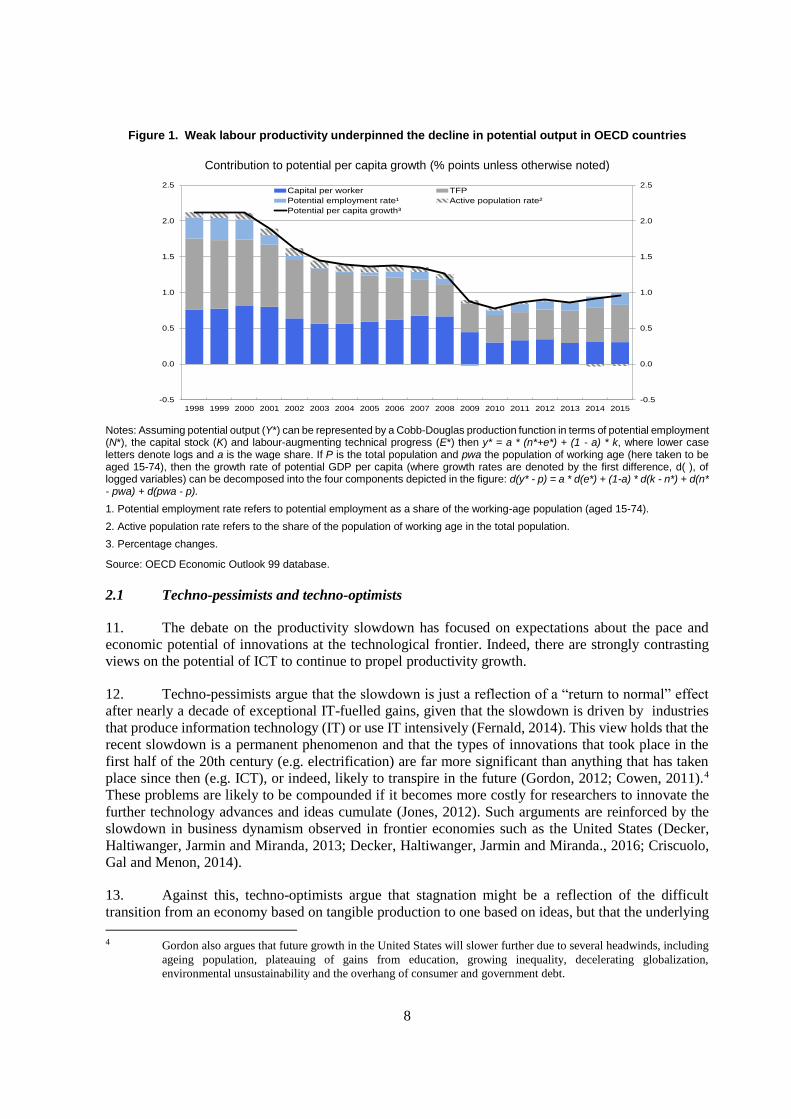
weakness in weak capital deepening (Figure 1). Against this background, this section reviews some of
the competing explanations for the productivity slowdown and places our research in the context of the
existing literature.
8
Figure 1. Weak labour productivity underpinned the decline in potential output in OECD countries
Contribution to potential per capita growth (% points unless otherwise noted)
Notes: Assuming potential output (Y*) can be represented by a Cobb-Douglas production function in terms of potential employment (N*), the capital stock (K) and labour-augmenting technical progress (E*) then y* = a * (n*+e*) + (1 - a) * k, where lower case letters denote logs and a is the wage share. If P is the total population and pwa the population of working age (here taken to be aged 15-74), then the growth rate of potential GDP per capita (where growth rates are denoted by the first difference, d( ), of logged variables) can be decomposed into the four components depicted in the figure: d(y* - p) = a * d(e*) + (1-a) * d(k - n*) + d(n* - pwa) + d(pwa - p).
1. Potential employment rate refers to potential employment as a share of the working-age population (aged 15-74).
2. Active population rate refers to the share of the population of working age in the total population.
3. Percentage changes.
Source: OECD Economic Outlook 99 database.
2.1 Techno-pessimists and techno-optimists
11. The debate on the productivity slowdown has focused on expectations about the pace and
economic potential of innovations at the technological frontier. Indeed, there are strongly contrasting
views on the potential of ICT to continue to propel productivity growth.
12. Techno-pessimists argue that the slowdown is just a reflection of a “return to normal” effect
after nearly a decade of exceptional IT-fuelled gains, given that the slowdown is driven by industries
that produce information technology (IT) or use IT intensively (Fernald, 2014). This view holds that the
recent slowdown is a permanent phenomenon and that the types of innovations that took place in the
first half of the 20th century (e.g. electrification) are far more significant than anything that has taken
place since then (e.g. ICT), or indeed, likely to transpire in the future (Gordon, 2012; Cowen, 2011).4
These problems are likely to be compounded if it becomes more costly for researchers to innovate the
further technology advances and ideas cumulate (Jones, 2012). Such arguments are reinforced by the
slowdown in business dynamism observed in frontier economies such as the United States (Decker,
Haltiwanger, Jarmin and Miranda, 2013; Decker, Haltiwanger, Jarmin and Miranda., 2016; Criscuolo,
Gal and Menon, 2014).
13. Against this, techno-optimists argue that stagnation might be a reflection of the difficult
transition from an economy based on tangible production to one based on ideas, but that the underlying
4 Gordon also argues that future growth in the United States will slower further due to several headwinds, including
ageing population, plateauing of gains from education, growing inequality, decelerating globalization,
environmental unsustainability and the overhang of consumer and government debt.
-0.5
0.0
0.5
1.0
1.5
2.0
2.5
-0.5
0.0
0.5
1.0
1.5
2.0
2.5
1998 1999 2000 2001 2002 2003 2004 2005 2006 2007 2008 2009 2010 2011 2012 2013 2014 2015
Capital per worker TFP
Potential employment rate¹ Active population rate²
Potential per capita growth³
9
rate of technological progress has not slowed and that the IT revolution will continue to dramatically
transform frontier economies. According to Brynjolfsson and McAfee (2011), the increasing
digitalization of economic activities has unleashed four main innovative trends: i) improved real-time
measurement of business activities; ii) faster and cheaper business experimentation; iii) more
widespread and easier sharing of ideas; and iv) the ability to replicate innovations with greater speed
and fidelity (scaling-up). While each of these trends are important in isolation, their impacts are
amplified when applied in unison.5 Similarly, Joel Mokyr argues that advances in computing power and
information and communication technologies have the potential to fuel future productivity growth by
making advances in basic science more likely and reducing access costs and thus igniting a virtuous
circle between technology and science. However, Mokyr warns of the potential for bad institutions and
policies to act as obstacles to this virtuous cycle.6
14. One interesting angle in the techno-optimist argument is that we might not have seen the full
benefits of the “digital economy” because we are still in a transition phase characterised by staggered
adoption of the new technology and transition costs. These transition dynamics are very much in line
with the idea that ICT is a General Purpose Technology (GPT) whose adoption and diffusion is
characterised by an S-curve (Griliches, 1957; David, 1991; Jovanovic and Rousseau, 2005). In
particular, GPT adoption and diffusion is complicated by a high cost of learning on how to use it
effectively; large adjustment costs and slow introduction of complementary inputs, especially
knowledge based capital (KBC). In fact, the productivity slowdown may reflect the dynamics associated
with these complementary investments (Fernald and Basu, 2006).
2.2 Macroeconomic factors
15. Although aggregate productivity slowed before the crisis in many economies, the debate has
also focused on the role of non-technology macroeconomic factors, namely demand, savings and
monetary policy. Accounts linking demand to the slowdown tend to emphasise “secular stagnation”,
whereby there is an imbalance between savings and investment caused by an increased propensity to
save and a decreasing propensity to invest which in turn leads to excessive savings dragging down
demand, lower real interest rates and a reduction in growth and inflation (Summers, 2016). Significant
growth, such as that characterizing the 2003-2007 boom, was achieved thanks to excessive levels of
borrowing and unsustainable investment levels.
16. Christiano, Eichenbaum and Trabandt (2015) analysed the role of macro shocks and financial
frictions during the crisis as triggers of the slowdown, but such models take the slowdown in MFP as
exogenous. Of more interest for our purposes is a recent paper by Anzoategui, Comin, Gertler and
Martinez (2016), which propose a theoretical model whereby the increase in demand for liquidity, as
observed during the crisis, increases the spread between the cost of capital and the risk-free rate of liquid
assets. This leads to a decline in investment in R&D and technological adoption, which in turn yields
lower output and lower MFP. According to the model, the spread of technology adoption varies over
the business cycle, with the cyclicality mainly driven by fluctuation in the adoption rate, which depends
5 For example, measurement is far more useful when coupled with active experimentation and knowledge sharing,
while the value of experimentation is proportionately greater if the benefits, in the event of success, can be leveraged
through rapid scaling-up.
6 According to Mokyr, potential barriers could come from: i) outright resistance by entrenched interests which could
lead to excess regulation and lack of entrepreneurial finance; ii) a poor institutional set up of research funding which
favours incremental as opposed to radical innovation; and iii) new forms of crime and insecurity (e.g. cyber
insecurity).
10
also on fiscal and monetary policies. The model, however, has to rely on exogenous medium term factors
to explain the pre-recession slowdown.
2.3 Rising resource misallocation
17. Gopinath, Kalemli-Ozcan, Karabarbounis and Villegas-Sanchez (2015) explore the
implications for sectoral MFP of the decline in real interest rate, observed in Southern Europe during
the euro-convergence process. They find that the associated capital inflow was increasingly misallocated
towards firms that had higher net worth but were not necessarily more productive, which could explain
why MFP slowed in Southern Europe – especially Spain – even before the crisis. This misallocation-
driven slowdown was further exacerbated by the additional uncertainty generated by the crisis and more
generally is likely to be related to weakening market selection, declining business dynamism and
deteriorating business investment.
2.4 Measurement issues
18. Finally, the debate had also raised the possibility that the productivity slowdown might have
just been a reflection of increasing mismeasurement of the gains from innovation in IT-related goods
and services.7 However recent analysis for the US (Byrne, Fernald and Reinsdorf 2016; and Syverson,
2016) suggests that this is highly unlikely (see recent Brookings brief by Derviş and Qureshi for an
overview). Given that IT producing sectors have seen rising import penetration and most of the IT
production is now done outside the US, the effect (either way) would be small and in no way large
enough to explain the slowdown observed in the US. In fact, “improving” measurement would, if
anything, make the slowdown more pronounced to the extent that US domestic production of these
products has fallen over the 1995-2004 period. Furthermore, mismeasurement of IT hardware is
significant already prior to the slowdown. Finally, the largest benefits of recent innovations in ICT go
to consumers in non-market production activities which again would not show up in GDP measures. In
fact, Syverson (2016) shows that the slowdown is not correlated with IT production or use.
2.5 Our contribution
19. In this paper, we aim to bring the debate on the global productivity slowdown – which has by
and large been conducted from a macroeconomic perspective – back to a more micro-level. While the
Gordon-Brynjolfsson controversy is essentially a debate about prospects at the global productivity
frontier, it is remarkable how little is actually known about the performance of firms that operate at the
global frontier. In this regard, we provide new evidence that highlights the importance of separately
considering what happens to innovation at the frontier as well as the diffusion of new and unexploited
existing technologies to laggards firms. This micro evidence is both key to motivating new theoretical
work and to shifting the debate to areas where there may be more traction for policy reforms to revive
productivity performance in OECD countries.
20. We show that a particularly striking feature of the productivity slowdown is not so much a
lower productivity growth at the global frontier, but rather rising labour productivity at the global
frontier coupled with an increasing labour productivity divergence between the global frontier and
laggard firms.8 This productivity divergence remains after controlling for differences in capital
7 See also the discussion in Ahmad and Schreyer (2016) on measuring GDP in a digitalised economy.
8 Preliminary results from the OECD Multiprod project (http://oe.cd/multiprod) based on the micro-aggregation of
official representative firm-level data for 15 countries over the last 20 years (Berlingieri, Blanchenay and Criscuolo,
2016) show that most countries have experienced growing labour and multi factor productivity dispersion coupled
11
deepening and mark-up behaviour although there is evidence that market power of frontier firms has
increased in services. This leads us to suspect that the rising MFPR gap between global frontier and
laggard firms may in fact reflect technological divergence.
21. MFP divergence could plausibly reflect the potential for structural changes in the global
economy – namely digitalisation, globalisation and the rising importance of tacit knowledge – to fuel
rapid productivity gains at the global frontier. Yet, aggregate MFP performance was significantly
weaker in industries where MFP divergence was more pronounced, suggesting that the divergence
observed is not solely driven by frontier firm pushing the boundary outward. In this regard, we contend
that increasing MFP divergence – and the global productivity slowdown more generally – could reflect
a slowdown in the technological diffusion process. This stagnation could be a reflection of increasing
costs for laggards firms of moving from an economy based on production to one based on ideas. But it
could also be symptomatic of rising entry barriers and a decline in the contestability of markets. In both
cases, public policy can play an important role in “alleviating” the productivity slowdown. Consistent
with this, we find the rise in MFP divergence to be much more extreme in sectors where pro-competitive
product market reforms were least extensive, suggesting that the observed rise in MFP divergence might
be at least partly due to policy weakness stifling diffusion and adoption in OECD economies.
22. Evidence of technological divergence at the firm level is significant in light of recent aggregate
level analysis suggesting that while adoption lags for new technologies across countries have fallen over
time, long-run penetration rates once technologies are adopted diverge across countries, with important
implications for cross-country income differences (Comin and Mestieri, 2013). More specifically, new
technologies developed at the global frontier are spreading more and more rapidly across countries but
their diffusion to all firms within any economy is slower and slower, with many available technologies
remaining unexploited by a non-trivial share of firms. A key implication is that weak productivity
performance in OECD countries may persist, unless a new wave of structural reforms can revive a
broken diffusion machine.
3. Data and identification of the global productivity frontier
23. This paper uses a harmonized firm-level productivity database, based on underlying data from
the recently updated OECD-Orbis database (see Gal, 2013). The database contains several productivity
with increased dispersion in marginal revenue product of capital (MRPK) allowing for non-constant returns to
scale. This rising productivity dispersion and misallocation is evident in both manufacturing and services, but is
generally much stronger in the services sector. Gamberoni, Giordano and Lopez-Garcia (2016) use micro-
aggregated firm-level data sources mainly based on firm level data from Central Banks compiled in the European
Central Bank’s CompNet project from 5 European countries and show increasing dispersion in MRPK and MRPL
across firms in the 2000s up to the crisis. Under their assumptions of constant returns to scale, MRPK and MRPL
are simply multiples of capital and labour productivity, hence their findings can also be interpreted as rising
divergence in productivity levels. They also find that dispersion is stronger amongst the services sectors. By
focusing on the frontier, our paper provides a discussion specifically on the upper half of the productivity
distribution.
12
measures (variants of labour productivity and multi-factor productivity, MFP) and covers to 24 OECD
countries9 over the period 1997 to 2014 for the non-farm, non-financial business sector.10
24. As discussed in Gal (2013), these data are sourced from annual balance sheet and income
statements, collected by Bureau van Dijk (BVD) – an electronic publishing firm – using a variety of
underlying sources ranging from credit rating agencies (Cerved in Italy) to national banks (National
Bank of Belgium for Belgium) as well as financial information providers (Thomson Reuters for the
US).11 It is the largest available cross-country company-level database for economic and financial
research. However, since the information is primarily collected for use in the private sector typically
with the aim of financial benchmarking, a number of steps need to be undertaken before the data can be
used for economic analysis. The steps we apply closely follow suggestions by Kalemli-Ozcan, Sorensen,
Villegas-Sanchez, Volosovych and Yesiltas (2015) and previous OECD experience (Gal, 2013; Ribeiro,
Menghinello and Backer, 2010).12 Three broad steps are: i) ensuring comparability of monetary variables
across countries and over time (industry-level PPP conversion and deflation); ii) deriving new variables
that will be used in the analysis (capital stock, productivity); and iii) keeping company accounts with
valid and relevant information for our present purposes (filtering or cleaning). Finally, Orbis is a
subsample of the universe of companies for most countries, retaining the larger and hence probably
more productive firms. To mitigate problems arising from this – particularly the under-representation of
small firms – we restrict our sample to firms with more than 20 employees on average over their
observed lifespan. For more details, see the sections in Appendix E on Data and on Representativeness
issues.
25. Further, a number of issues that commonly affect productivity measurement should be kept in
mind. First, differences in the quality and utilisation of capital and labour inputs cannot be accounted
for as the capital stock is measured in book values and labour input by the number of employees.13
Secondly, measuring outputs and inputs in internationally comparable price levels remains an important
challenge.14 Finally, similar to most firm-level datasets, Orbis contains variables on outputs and inputs
in nominal values and no additional separate information on firm-specific prices and quantities (i.e. we
observe total sales of steel bars, but no information on tonnes of steel bars sold and price per ton), thus
output is proxied by total revenues or total value added. Even though we deflate these output measures
by country-industry-year level deflators (at the 2-digit detail), differences in measured (revenue)
9 These countries are: Austria, Belgium, Czech Republic, Denmark, Estonia, Finland, France, Germany, Great
Britain, Greece, Hungary, Ireland, Italy, Japan, Korea, Netherlands, Norway, Poland, Portugal, Spain, Sweden,
Slovenia, the Slovak Republic and the United States. The country coverage is somewhat smaller in the policy
analysis.
10 This means retaining industries with 2 digit codes from 5 to 82, excluding 64-66 in the European classification
system NACE Rev 2, which is equivalent to the international classification system ISIC Rev. 4 at the 2-digit level.
11 See the full list of information providers to Bureau van Dijk regarding financial information for the set of countries
retained in the analysis in Appendix E.
12 We are grateful for Sebnem Kalemli-Ozcan and Sevcan Yesiltas for helpful discussions about their experience and
suggestions with the Orbis database.
13 The measurement of intangible fixed assets in the balance sheets follows accounting rules, hence the total fixed
assets (sum of tangibles and intangibles) may understate the overall capital stock (Corrado et al, 2009). Moreover,
different depreciation rates and investment price deflators cannot be applied, since an asset type breakdown is not
available. The implications of these limitations will be discussed in Section 4.2 where we analyse the patterns found
in the data.
14 We use the country-industry level purchasing power parity database of Inklaar and Timmer (2014), see details
therein for the tradeoffs involved in deriving their PPP measures.
13
productivity across firms within a given industry may still reflect both differences in technology as well
as differences in market power.15 As described below, we attempt to correct our productivity measures
for differences in market power by deriving firm- and time- specific mark-ups following De Loecker
and Warzynski (2012).
3.1 Productivity measurement
26. As a starting point, we focus on labour productivity, which is calculated by dividing real value
added (in US 2005 PPP that vary by industry) by the number of employees. Using labour productivity
has the advantage that it retains the largest set of observations, as it does not require the availability of
measures for fixed assets or intermediate inputs (proxied by materials) potentially used for deriving
multi-factor productivity (MFP). Our baseline MFP relies on a value added based production function
estimation with the number of employees and real capital as inputs. We employ the one-step GMM
estimation method proposed by Wooldridge (2009), which mitigates the endogeneity problem of input
choices by using material inputs as proxy variables for productivity and (twice) lagged values of labour
as instruments. The production function is estimated separately for each 2-digit industry but pooled
across all countries, controlling for country and year fixed effects. This allows for inherent technological
differences across industries, while at the same time ensures comparability of MFP levels across
countries and over time by having a uniform labour and capital coefficient along these dimensions. For
more details, see Appendix E.
3.2 Correcting for mark-ups
27. In order to mitigate the limitations from not observing firm-level prices, we correct our revenue
based MFP measure by firm- and time-varying mark-ups. In order to do that, we apply the mark-up
estimation methodology of De Loecker and Warzynski (2012). We introduce a notation for the
“standard” MFP estimates as MFPR (denoting revenue based productivity) and the mark-up corrected
MFP estimates as 𝑀𝐹𝑃𝑅𝑐 , and we define it for each firm i and year t as follows:
𝑀𝐹𝑃𝑅𝑖𝑡𝑐 = 𝑀𝐹𝑃𝑅𝑖𝑡 − log(𝜇𝑖𝑡) ,
where the MFP values are measured in logs and 𝜇 denotes the estimated mark-up. The 𝑀𝐹𝑃𝑅𝑐 measure
provides an estimate for productivity that is purged from mark-up variations and hence is not
influenced by market power changes under the assumption that at least one input of production is fully
flexible (e.g. labour or materials) .16
28. The mark-up is derived from the supply-side approach originally proposed by Hall (1986) and
more recently re-explored by De Loecker and Warzynski (2012). As described in De Loecker and
15 In the above example, it is unclear whether revenue based productivity is higher because the firm is producing more
steel bars, or whether the firm’s higher observed productivity is driven by higher prices reflecting high mark-ups,
which the firm can charge because of a lack of competition, for example.
16 A further step would be a separation of market power and quality and/or demand. See Foster et al. (2008) and
Forlani et al (2016) on a related discussion about the role of different business strategies and their impact on
measured productivity through the example of Nissan (high number of produced cars into the cheaper segment)
and Mercedes (lower number of cars produced into the premium segment). Even if firm level prices were observed,
complications would still arise – see Byrne and Corrado (2015) who demonstrate that official output prices of
communication products are significantly under-estimated due to ignoring some quality improvements.
Haltiwanger (2016) discusses in great detail the various types of MFP calculations and to what extent they are
influenced by demand and market frictions.
14
Warzynski (2012), the approach computes mark-ups without needing assumptions about the demand
function, but only relying on available information on output and inputs, under the assumptions that at
least one input is fully flexible and that firms minimize costs. Thus, the mark-up – defined as the ratio
of the output price P over marginal cost MC – is derived from the first order condition of the plant’s cost
minimization problem with respect to the flexible input k as:
𝜇𝑖𝑡 =𝑃𝑖𝑡
𝑀𝐶𝑖𝑡= 𝑂𝑢𝑡𝑝𝑢𝑡 𝐸𝑙𝑎𝑠𝑡𝑖𝑐𝑖𝑡𝑦𝑖𝑘𝑡 𝑂𝑢𝑡𝑝𝑢𝑡 𝑆ℎ𝑎𝑟𝑒𝑖𝑘𝑡⁄ ,
That is, the mark-up of firm i at time t can be computed as the ratio between the elasticity of output17
with respect to the flexible input k (estimated in a first step) and flexible input k shares in output
(observed in the data). In our baseline specification, we use labour (as opposed to materials) as flexible
input to ensure the largest coverage of countries in our baseline specification. Thus mark-ups are
calculated as the ratio between the estimated production function parameter for labour �̂�𝐿𝑗 in industry j
where firm i operates and the “corrected” wage share 𝑤𝑠𝑖𝑡 =WLit
VAit̃:
𝜇𝑖𝑡 =�̂�𝐿
𝑗
𝑤𝑠𝑖𝑡.
29. The labour coefficient �̂�𝐿𝑗 in the numerator is estimated using the GMM estimation method
by Wooldridge (2009). The denominator is obtained by using a prediction of firm-level value added by
a rich polynomial function of observable inputs in order to retain only the anticipated part of output
developments.18 The rationale for using this correction is the assumption that firms do not observe
unanticipated shocks to production when making optimal input decisions.
30. Given potential criticisms that labour input may not be fully flexible – especially in countries
with rigid labour markets – we also calculated mark-ups using materials as the fully flexible input for a
subset of 18 countries for which data are available. In that case, a gross-output based production function
is estimated to obtain a coefficient for materials, again following Wooldridge (2009). As shown in
Appendix A, the main result of a strong divergence in MFP is robust to these different choices.
31. As De Loecker and van Biesebroeck (2016: 25) note, the intuition behind this mark-up
measure is as follows:
“Holding other inputs constant, a competitive firm will expand its use of [the flexible input, i.e.
labour] until the revenue share equals the output elasticity [hence the mark-up measure would be
1]. […] If a firm does not increase [its flexible input use] all the way until equality holds, but
prefers to produce a lower quantity and raise the output price instead, it indicates the firm is able
to exercise market power and charge a price above marginal cost.”
32. As noted in De Loecker and Warzynski (2012), the low demand in terms of additional
assumptions of their approach and the lack of information on firm level prices bear some costs. Given
that we do not observe firms’ physical output, the approach is only informative on the way mark-ups
17 Note that for simplicity we have assumed that the firm only produces one product. In the case of multiproduct firms,
one should calculate mark-ups for each of the products sold by the firm.
18 The polynomial includes all possible interactions between labour, capital and materials containing first and second
degree terms, along with first and second degree base effects. This follows the Stata code provided by De Loecker
and Warzynski (2012) with their online Appendix, with the difference that for computational reasons we omitted
that third degree terms.
15
change over time (not their level) and in relative terms, i.e. on the correlation with firm characteristics
(e.g. productivity, size, export status) rather than in absolute levels. In what follows therefore, we will
look at relative trends in mark-ups for frontier and laggard firms.
3.3 Measuring the productivity frontier
33. In keeping with the (scarce) existing literature (Bartelsman, Haskel and Martin, 2008; Crespi
and Iacovello, 2010; Arnold, Nicoletti and Scarpetta, 2011), we define the global productivity frontier
as the top 5% of firms in terms of productivity levels, within each industry and year. As there is a
tendency in Orbis for the number of firms (with available data to calculate productivity) to expand over
time, we slightly deviate from this practice in our preferred definition of frontier firms.19 One implication
of the increasing coverage of Orbis over time is that smaller – and presumably less productive – firms
get included in the frontier in the latter years of the sample. Thus, the evolution of the top 5% on the
expanding Orbis sample could artificially underestimate average productivity at the frontier over time
just as a reflection of the expanding sample. To avoid this, we calculate the 5% of firms per industry
using a fixed number of firms across time. This circumvents the expanding coverage problem but still
allows for differences across industries in terms of their firm population, which is important given the
heterogeneity of average firm size across industries. More specifically, frontier firms are identified using
the top 5% of the median number of firms (across years), separately by each industry. This approach
aims to capture as close as possible the top 5% of the typical population of firms. Using a MFPR-based
productivity frontier definition, for example, results in a global frontier size of about 80 companies for
the typical 2-digit industry.20
34. Importantly, however, while the number of frontier firms is fixed, the set of frontier firms is
allowed to change over time. This choice is necessary to ensure that when assessing the evolution of the
frontier, we account for the phenomenon of turbulence at the top: some firms can become highly
productive and push the frontier, while other, previously productive, businesses can lose their
advantages and fall out of the frontier. This will not necessarily lead to a bias where the frontier becomes
relatively more productive over time, however, since the composition of the laggard grouping is also
allowed to change, the average productivity of this grouping could also in principle be boosted the entry
(exit) of more (less) productive firms.21 As discussed in Section 4.4, while there is churning at the
frontier, this is largely concentrated amongst the top quintile of the productivity distribution.
3.4 Characteristics of frontier firms
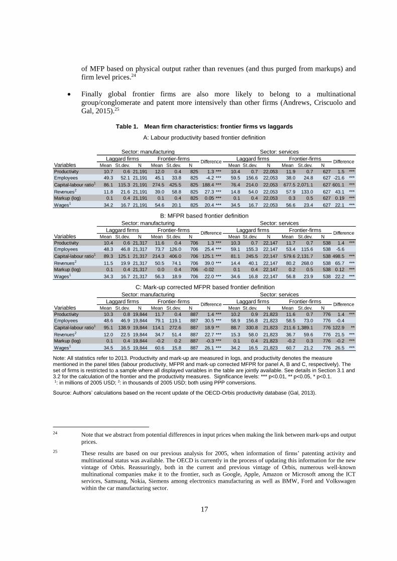
35. Table 1 reports cross-sectional differences in average characteristics for global frontier firms
relative to non-frontier firms along a number of measurable dimensions, focusing on the last year of our
sample, 2013. Panel A reports these differences based on a labour productivity measure while Panel B
19 In Andrews et al, 2015, we adopted a definition based on a fixed number of firms across time as well as across
industries (top 100 or top 50). By allowing the frontier size to vary across industries, we better tailor the frontier
definition to each industry. As Figure A3 in Appendix A shows, the choice among these alternatives does not affect
the main finding of a growing productivity gap between the frontier and the rest.
20 The number of firms at the global frontier is 83 for the median industry (i.e. manufacture of basic metals). For the
industries populated with a large number of businesses, the frontier represents about 400-500 companies (e.g. retail
and wholesale trade, construction).
21 The empirical literature on productivity-enhancing reallocations can indeed find an important role for the entry-
exit margin of firms (e.g. Foster et al., 2001), and the theoretical literature also emphasizes its potential role
(Caballero and Hammour, 1994; Campbell, 1998).

16
does likewise using MFPR and Panel C using mark-up corrected MFPR. A few interesting facts emerge
from the tables.
First, firms at the global productivity frontier are on average 3 to 4 times more productive than
non-frontier firms.22 At first glance, these differences appear large but are to be expected given
the widespread heterogeneity in firm productivity that is typically observed within narrowly
defined sectors (Syverson, 2004).23A host of literature has focused on how such large
differences in productivity can be sustained in equilibrium, given the expectation that market
selection and the reallocation of resources would necessarily equalise them over the longer
run. Supply-side explanations have typically emphasised factors related to technology shocks,
management skill, R&D, or investment patterns (Bartelsman and Doms, 2000). The demand
side also appear relevant, given evidence that imperfect product substitutability – due to
geographical segmentation (i.e. transport costs), product differentiation (i.e. consumer
preferences, branding/advertising) and intangible factors (customer-producer relationships) –
can prevent industry customers from easily shifting purchases between industry producers
(Syverson, 2004). The combination of demand and supply side imperfections can indeed lead
to large and persistent differences in productivity levels across firms (Syverson, 2011). Note
that most studies focus on within-country productivity dispersion, while our analysis pools
together different countries, potentially further widening the productivity distribution.
Second, on average, global frontier firms have larger sales and are more capital intensive –as
expected, more so for labour productivity. However, frontier firms do not employ a
significantly larger number of employees in services for any of the productivity measures
analysed.
Third, global frontier firms pay higher wages, which ranges between $20,000 and $26,000 (in
2005 USD terms) depending on the measure. These differences might reflect the sorting of
better workers into frontier firms (Card, Heining and Kline, 2013; Song, Price, Guvenen,
Bloom and von Wachter, 2016) and the potential sharing of higher rents by frontier companies
with their workers.
Fourth, in manufacturing, firms at the frontier in terms of MFP (MFPR and its mark-up
corrected variant) have significantly higher employment size than laggards, in line with
existing evidence that productivity is positively correlated with size of manufacturing firms.
Fifth, frontier firms are also shown to charge higher mark-ups in the case of labour productivity
and MFPR, particularly in services. This could reflect weaker competition in the less tradable
and more regulated services sector, which allows for larger market power differences across
firms. However, when the frontier is defined based on mark-up corrected MFPR, frontier firms
are found to charge lower mark-ups. This is consistent with the idea that the most productive
firms can afford to charge lower prices and thus attract more demand. In particular, this is in
line with the findings of Foster, Haltiwanger and Syverson (2008) using US firm level data on
prices and quantities, who show that there is a strong negative relationship between measures
22 Note that productivity is measured in logs, so relative to laggard firms, global frontier firms are exp1.3=3.6 times
more productive.
23 For example, within 4 digit manufacturing industries in the United States, Syverson (2004) finds a 2-to-1 ratio in
value added per worker between the 75th- and 25th-percentile plants in an industry’s productivity distribution.
Including more of the tails of the distribution amplifies the dispersion, with the average 90–10 and 95–5 percentile
labour productivity ratios within industries in excess of 4-to-1 and 7-to-1, respectively.
17
of MFP based on physical output rather than revenues (and thus purged from markups) and
firm level prices.24
Finally global frontier firms are also more likely to belong to a multinational
group/conglomerate and patent more intensively than other firms (Andrews, Criscuolo and
Gal, 2015).25
Table 1. Mean firm characteristics: frontier firms vs laggards
A: Labour productivity based frontier definition
B: MFPR based frontier definition
C: Mark-up corrected MFPR based frontier definition
Note: All statistics refer to 2013. Productivity and mark-up are measured in logs, and productivity denotes the measure mentioned in the panel titles (labour productivity, MFPR and mark-up corrected MFPR for panel A, B and C, respectively). The set of firms is restricted to a sample where all displayed variables in the table are jointly available. See details in Section 3.1 and 3.2 for the calculation of the frontier and the productivity measures. Significance levels: *** p<0.01, ** p<0.05, * p<0.1. 1: in millions of 2005 USD; 2: in thousands of 2005 USD; both using PPP conversions.
Source: Authors’ calculations based on the recent update of the OECD-Orbis productivity database (Gal, 2013).
24 Note that we abstract from potential differences in input prices when making the link between mark-ups and output
prices.
25 These results are based on our previous analysis for 2005, when information of firms’ patenting activity and
multinational status was available. The OECD is currently in the process of updating this information for the new
vintage of Orbis. Reassuringly, both in the current and previous vintage of Orbis, numerous well-known
multinational companies make it to the frontier, such as Google, Apple, Amazon or Microsoft among the ICT
services, Samsung, Nokia, Siemens among electronics manufacturing as well as BMW, Ford and Volkswagen
within the car manufacturing sector.
Variables Mean St.dev. N Mean St.dev. N Mean St.dev. N Mean St.dev. N
Productivity 10.7 0.6 21,191 12.0 0.4 825 1.3 *** 10.4 0.7 22,053 11.9 0.7 627 1.5 ***
Employees 49.3 52.1 21,191 45.1 33.8 825 -4.2 *** 59.5 156.6 22,053 38.0 24.8 627 -21.6 ***
Capital-labour ratio1 86.1 115.3 21,191 274.5 425.5 825 188.4 *** 76.4 214.0 22,053 677.5 2,071.1 627 601.1 ***
Revenues2 11.8 21.6 21,191 39.0 58.8 825 27.3 *** 14.8 54.0 22,053 57.9 133.0 627 43.1 ***
Markup (log) 0.1 0.4 21,191 0.1 0.4 825 0.05 *** 0.1 0.4 22,053 0.3 0.5 627 0.19 ***
Wages1 34.2 16.7 21,191 54.6 20.1 825 20.4 *** 34.5 16.7 22,053 56.6 23.4 627 22.1 ***
Difference DifferenceLaggard firms Frontier-firms
Sector: manufacturing Sector: services
Laggard firms Frontier-firms
Variables Mean St.dev. N Mean St.dev. N Mean St.dev. N Mean St.dev. N
Productivity 10.4 0.6 21,317 11.6 0.4 706 1.3 *** 10.3 0.7 22,147 11.7 0.7 538 1.4 ***
Employees 48.3 46.8 21,317 73.7 126.0 706 25.4 *** 59.1 155.3 22,147 53.4 115.6 538 -5.6
Capital-labour ratio1 89.3 125.1 21,317 214.3 406.0 706 125.1 *** 81.1 245.5 22,147 579.6 2,131.7 538 498.5 ***
Revenues2 11.5 19.9 21,317 50.5 74.1 706 39.0 *** 14.4 40.1 22,147 80.2 268.0 538 65.7 ***
Markup (log) 0.1 0.4 21,317 0.0 0.4 706 -0.02 0.1 0.4 22,147 0.2 0.5 538 0.12 ***
Wages1 34.3 16.7 21,317 56.3 18.9 706 22.0 *** 34.6 16.8 22,147 56.8 23.9 538 22.2 ***
Difference DifferenceLaggard firms Frontier-firms
Sector: manufacturing Sector: services
Laggard firms Frontier-firms
Variables Mean St.dev. N Mean St.dev. N Mean St.dev. N Mean St.dev. N
Productivity 10.3 0.8 19,844 11.7 0.4 887 1.4 *** 10.2 0.9 21,823 11.6 0.7 776 1.4 ***
Employees 48.6 46.9 19,844 79.1 119.1 887 30.5 *** 58.9 156.8 21,823 58.5 73.0 776 -0.4
Capital-labour ratio1 95.1 138.9 19,844 114.1 272.6 887 18.9 ** 88.7 330.8 21,823 211.6 1,389.1 776 122.9 **
Revenues2 12.0 22.5 19,844 34.7 51.4 887 22.7 *** 15.3 58.0 21,823 36.7 59.6 776 21.5 ***
Markup (log) 0.1 0.4 19,844 -0.2 0.2 887 -0.3 *** 0.1 0.4 21,823 -0.2 0.3 776 -0.2 ***
Wages1 34.5 16.5 19,844 60.6 15.8 887 26.1 *** 34.2 16.5 21,823 60.7 21.2 776 26.5 ***
Difference DifferenceLaggard firms Frontier-firms
Sector: manufacturing Sector: services
Laggard firms Frontier-firms
18
4. Productivity divergence between the global frontier and laggard firms
4.1 Labour productivity divergence
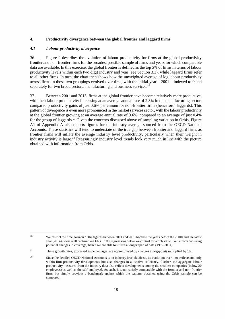
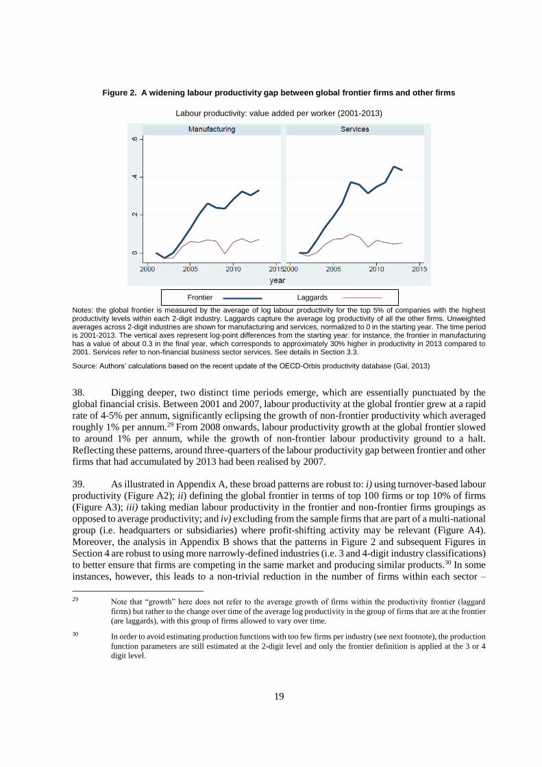
36. Figure 2 describes the evolution of labour productivity for firms at the global productivity
frontier and non-frontier firms for the broadest possible sample of firms and years for which comparable
data are available. In this exercise, the global frontier is defined as the top 5% of firms in terms of labour
productivity levels within each two digit industry and year (see Section 3.3), while laggard firms refer
to all other firms. In turn, the chart then shows how the unweighted average of log labour productivity
across firms in these two groupings evolved over time, with the initial year – 2001 – indexed to 0 and
separately for two broad sectors: manufacturing and business services.26
37. Between 2001 and 2013, firms at the global frontier have become relatively more productive,
with their labour productivity increasing at an average annual rate of 2.8% in the manufacturing sector,
compared productivity gains of just 0.6% per annum for non-frontier firms (henceforth laggards). This
pattern of divergence is even more pronounced in the market services sector, with the labour productivity
at the global frontier growing at an average annual rate of 3.6%, compared to an average of just 0.4%
for the group of laggards.27 Given the concerns discussed above of sampling variation in Orbis, Figure
A1 of Appendix A also reports figures for the industry average sourced from the OECD National
Accounts. These statistics will tend to understate of the true gap between frontier and laggard firms as
frontier firms will inflate the average industry level productivity, particularly when their weight in
industry activity is large.28 Reassuringly industry level trends look very much in line with the picture
obtained with information from Orbis.
26 We restrict the time horizon of the figures between 2001 and 2013 because the years before the 2000s and the latest
year (2014) is less well captured in Orbis. In the regressions below we control for a rich set of fixed effects capturing
potential changes in coverage, hence we are able to utilize a longer span of data (1997-2014).
27 These growth rates, expressed in percentages, are approximated by changes in log-points multiplied by 100.
28 Since the detailed OECD National Accounts is an industry level database, its evolution over time reflects not only
within-firm productivity developments but also changes in allocative efficiency. Further, the aggregate labour
productivity measures from the industry data also reflect developments among the smallest companies (below 20
employees) as well as the self-employed. As such, it is not strictly comparable with the frontier and non-frontier
firms but simply provides a benchmark against which the patterns obtained using the Orbis sample can be
compared.
19
Figure 2. A widening labour productivity gap between global frontier firms and other firms
Labour productivity: value added per worker (2001-2013)
Notes: the global frontier is measured by the average of log labour productivity for the top 5% of companies with the highest productivity levels within each 2-digit industry. Laggards capture the average log productivity of all the other firms. Unweighted averages across 2-digit industries are shown for manufacturing and services, normalized to 0 in the starting year. The time period is 2001-2013. The vertical axes represent log-point differences from the starting year: for instance, the frontier in manufacturing has a value of about 0.3 in the final year, which corresponds to approximately 30% higher in productivity in 2013 compared to 2001. Services refer to non-financial business sector services. See details in Section 3.3.
Source: Authors’ calculations based on the recent update of the OECD-Orbis productivity database (Gal, 2013)
38. Digging deeper, two distinct time periods emerge, which are essentially punctuated by the
global financial crisis. Between 2001 and 2007, labour productivity at the global frontier grew at a rapid
rate of 4-5% per annum, significantly eclipsing the growth of non-frontier productivity which averaged
roughly 1% per annum.29 From 2008 onwards, labour productivity growth at the global frontier slowed
to around 1% per annum, while the growth of non-frontier labour productivity ground to a halt.
Reflecting these patterns, around three-quarters of the labour productivity gap between frontier and other
firms that had accumulated by 2013 had been realised by 2007.
39. As illustrated in Appendix A, these broad patterns are robust to: i) using turnover-based labour
productivity (Figure A2); ii) defining the global frontier in terms of top 100 firms or top 10% of firms
(Figure A3); iii) taking median labour productivity in the frontier and non-frontier firms groupings as
opposed to average productivity; and iv) excluding from the sample firms that are part of a multi-national
group (i.e. headquarters or subsidiaries) where profit-shifting activity may be relevant (Figure A4).
Moreover, the analysis in Appendix B shows that the patterns in Figure 2 and subsequent Figures in
Section 4 are robust to using more narrowly-defined industries (i.e. 3 and 4-digit industry classifications)
to better ensure that firms are competing in the same market and producing similar products.30 In some
instances, however, this leads to a non-trivial reduction in the number of firms within each sector –
29 Note that “growth” here does not refer to the average growth of firms within the productivity frontier (laggard
firms) but rather to the change over time of the average log productivity in the group of firms that are at the frontier
(are laggards), with this group of firms allowed to vary over time.
30 In order to avoid estimating production functions with too few firms per industry (see next footnote), the production
function parameters are still estimated at the 2-digit level and only the frontier definition is applied at the 3 or 4
digit level.
Frontier Laggards
20
raising difficulties for production function estimation and increasing the prevalence of idiosyncratic and
noisy patterns. This leads us to conduct our baseline analysis at the two-digit level.31
4.2 Labour productivity divergence: capital deepening or MFP?
40. Since gains in labour productivity at the firm level can be achieved through either higher
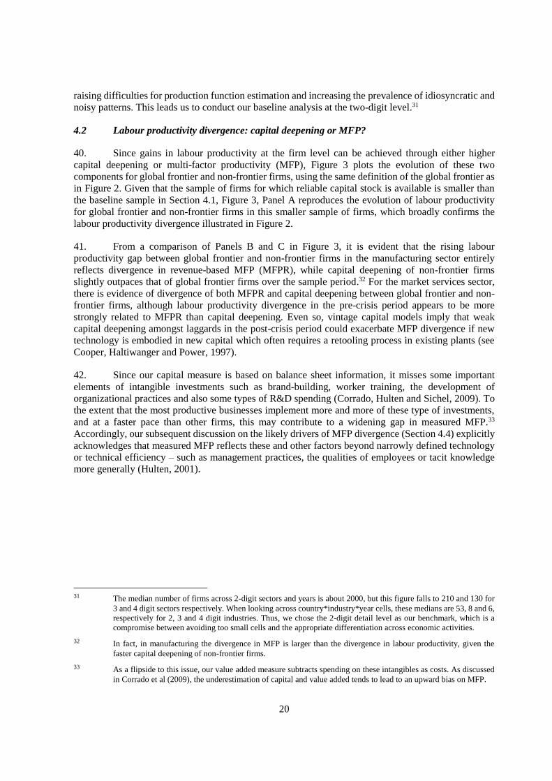
capital deepening or multi-factor productivity (MFP), Figure 3 plots the evolution of these two
components for global frontier and non-frontier firms, using the same definition of the global frontier as
in Figure 2. Given that the sample of firms for which reliable capital stock is available is smaller than
the baseline sample in Section 4.1, Figure 3, Panel A reproduces the evolution of labour productivity
for global frontier and non-frontier firms in this smaller sample of firms, which broadly confirms the
labour productivity divergence illustrated in Figure 2.
41. From a comparison of Panels B and C in Figure 3, it is evident that the rising labour
productivity gap between global frontier and non-frontier firms in the manufacturing sector entirely
reflects divergence in revenue-based MFP (MFPR), while capital deepening of non-frontier firms
slightly outpaces that of global frontier firms over the sample period.32 For the market services sector,
there is evidence of divergence of both MFPR and capital deepening between global frontier and non-
frontier firms, although labour productivity divergence in the pre-crisis period appears to be more
strongly related to MFPR than capital deepening. Even so, vintage capital models imply that weak
capital deepening amongst laggards in the post-crisis period could exacerbate MFP divergence if new
technology is embodied in new capital which often requires a retooling process in existing plants (see
Cooper, Haltiwanger and Power, 1997).
42. Since our capital measure is based on balance sheet information, it misses some important
elements of intangible investments such as brand-building, worker training, the development of
organizational practices and also some types of R&D spending (Corrado, Hulten and Sichel, 2009). To
the extent that the most productive businesses implement more and more of these type of investments,
and at a faster pace than other firms, this may contribute to a widening gap in measured MFP.33
Accordingly, our subsequent discussion on the likely drivers of MFP divergence (Section 4.4) explicitly
acknowledges that measured MFP reflects these and other factors beyond narrowly defined technology
or technical efficiency – such as management practices, the qualities of employees or tacit knowledge
more generally (Hulten, 2001).
31 The median number of firms across 2-digit sectors and years is about 2000, but this figure falls to 210 and 130 for
3 and 4 digit sectors respectively. When looking across country*industry*year cells, these medians are 53, 8 and 6,
respectively for 2, 3 and 4 digit industries. Thus, we chose the 2-digit detail level as our benchmark, which is a
compromise between avoiding too small cells and the appropriate differentiation across economic activities.
32 In fact, in manufacturing the divergence in MFP is larger than the divergence in labour productivity, given the
faster capital deepening of non-frontier firms.
33 As a flipside to this issue, our value added measure subtracts spending on these intangibles as costs. As discussed
in Corrado et al (2009), the underestimation of capital and value added tends to lead to an upward bias on MFP.
21
Figure 3. The widening labour productivity gap is mainly driven by MFP divergence
A: Labour Productivity
B: Multi-Factor Productivity (MFPR)
C: Capital deepening
Notes: the global frontier group of firms is defined by the top 5% of companies with the highest productivity levels within each 2-digit industry. Laggards capture all the other firms. Unweighted averages across 2-digit industries are shown for log labour productivity, the Wooldridge (2009) type production-function based log MFPR measure and the log of real capital stock over employment for Panels A, B and C, respectively, separately for manufacturing and services, normalized to 0 in the starting year. Time period is 2001-2013. Services refer to non-financial business services. See details in Section 3.3. The sample is restricted to those companies that have data available so as to measure capital stock and MFP. MFP (Panel B) and capital deepening
(Panel C) do not sum to labour productivity (Panel A) in a simple way. That is because 𝑉𝐴 / 𝐿 = 𝑀𝐹𝑃 (𝐾𝑎 𝐿𝑏 ) / 𝐿 =
𝑀𝐹𝑃 (𝐾
𝐿)
𝑎
𝐿𝑎+𝑏−1, where the capital coefficient (a) and the labour coefficient (b) are allowed to vary by industry.
Source: Authors’ calculations based on the recent update of the OECD-Orbis productivity database (Gal, 2013)
Frontier Laggards
22
4.3 MFP divergence: mark-ups or technology?
43. While evidence of divergence in MFP points towards a technological explanation of the rising
labour productivity gap between global frontier and other firms, it might also reflect the increasing
market power of frontier firms, given that our measure of multifactor productivity MFPR is based on
information on revenues. If the increasing differences in MFPR between frontier and laggards reflect
unobserved differences in firm level prices, the rising gap between global frontier and other firms in
MFPR may simply reflect the increasing ability of frontier firms to charge higher mark-ups, and thus
profitability as opposed to differences in technical efficiency. Accordingly, we attempt to assess the
contribution of mark-up behaviour to MFPR divergence, using the methodology outlined in Section 3.
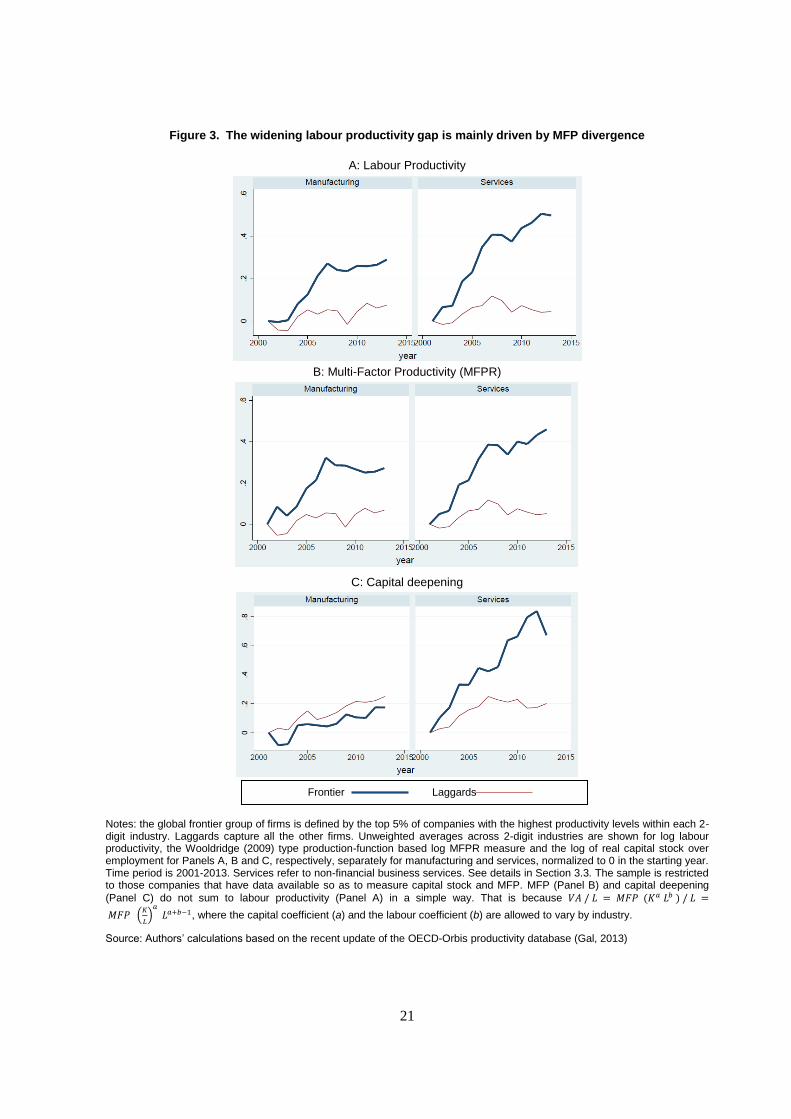
44. Given the focus on MFPR, the global frontier in Figure 4 is redefined in terms of the top 5%
of firms in terms of MFPR levels within each two digit industry and year. Using such a definition, the
divergence of MFPR in Figure 4, Panel A is very similar to that in Figure 3, Panel B, which defines the
global frontier in terms of labour productivity. These patterns are robust to using alternative definitions
of MFPR, based on a Solow residual or the Wooldridge gross-output estimation approach (Figure A6)
and to using materials (a proxy for intermediate inputs) as the fully flexible input in De Loecker and
Warzynski (2012) methodology for a subset of 18 countries for which data are available (Figure A8).
45. Figure 4, Panel B plots the evolution of the unweighted average of the estimated mark-ups for
global frontier and non-frontier firms. While estimates are quite volatile, the pre-crisis divergence in
MFPR in the manufacturing sector does not appear to be driven by frontier firms charging increasingly
higher mark-ups, relative to non-frontier firms. Turning to the services sector, there is evidence that
frontier firms increased their mark-ups relative to non-frontier firms in the pre-crisis period, in particular
after 2005, but this divergence in mark-up behaviour is significantly unwound in the post-crisis period.
Still, their mark-up levels are significantly higher than those of non-frontier firms (Table 1, Panel B).
Once we correct MFPR for these patterns in mark-ups, the divergence in mark-up corrected MFPR
between frontier and non-frontier firms in the pre-crisis is reduced by a factor of about one-third, while
the divergence becomes somewhat larger in recent years (Figure 4, Panel C).
23
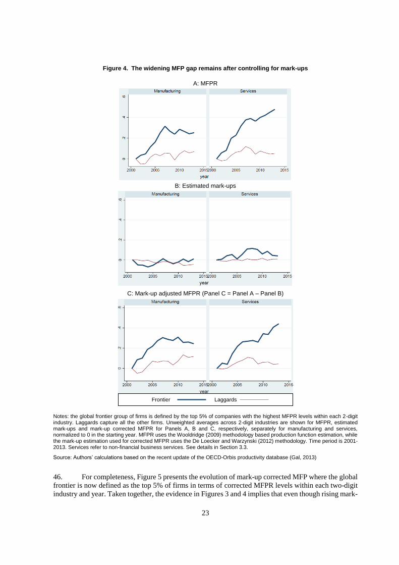
Figure 4. The widening MFP gap remains after controlling for mark-ups
A: MFPR
B: Estimated mark-ups
C: Mark-up adjusted MFPR (Panel C = Panel A – Panel B)
Notes: the global frontier group of firms is defined by the top 5% of companies with the highest MFPR levels within each 2-digit industry. Laggards capture all the other firms. Unweighted averages across 2-digit industries are shown for MFPR, estimated mark-ups and mark-up corrected MFPR for Panels A, B and C, respectively, separately for manufacturing and services, normalized to 0 in the starting year. MFPR uses the Wooldridge (2009) methodology based production function estimation, while the mark-up estimation used for corrected MFPR uses the De Loecker and Warzynski (2012) methodology. Time period is 2001-2013. Services refer to non-financial business services. See details in Section 3.3.
Source: Authors’ calculations based on the recent update of the OECD-Orbis productivity database (Gal, 2013)
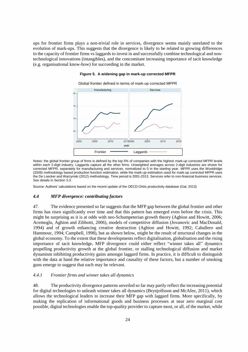
46. For completeness, Figure 5 presents the evolution of mark-up corrected MFP where the global
frontier is now defined as the top 5% of firms in terms of corrected MFPR levels within each two-digit
industry and year. Taken together, the evidence in Figures 3 and 4 implies that even though rising mark-
Frontier Laggards
24
ups for frontier firms plays a non-trivial role in services, divergence seems mainly unrelated to the
evolution of mark-ups. This suggests that the divergence is likely to be related to growing differences
in the capacity of frontier firms vs laggards to invest in and successfully combine technological and non-
technological innovations (intangibles), and the concomitant increasing importance of tacit knowledge
(e.g. organisational know-how) for succeeding in the market.
Figure 5. A widening gap in mark-up corrected MFPR
Global frontier defined in terms of mark-up corrected MFPR
Notes: the global frontier group of firms is defined by the top 5% of companies with the highest mark-up corrected MFPR levels within each 2-digit industry. Laggards capture all the other firms. Unweighted averages across 2-digit industries are shown for corrected MFPR, separately for manufacturing and services, normalized to 0 in the starting year. MFPR uses the Wooldridge (2009) methodology based production function estimation, while the mark-up estimation used for mark-up corrected MFPR uses the De Loecker and Warzynski (2012) methodology. Time period is 2001-2013. Services refer to non-financial business services. See details in Section 3.3.
Source: Authors’ calculations based on the recent update of the OECD-Orbis productivity database (Gal, 2013)
4.4 MFP divergence: contributing factors
47. The evidence presented so far suggests that the MFP gap between the global frontier and other
firms has risen significantly over time and that this pattern has emerged even before the crisis. This
might be surprising as it is at odds with neo-Schumpeterian growth theory (Aghion and Howitt, 2006;
Acemoglu, Aghion and Zilibotti, 2006), models of competitive diffusion (Jovanovic and MacDonald,
1994) and of growth enhancing creative destruction (Aghion and Howitt, 1992; Caballero and
Hammour, 1994; Campbell, 1998), but as shown below, might be the result of structural changes in the
global economy. To the extent that these developments reflect digitalisation, globalisation and the rising
importance of tacit knowledge, MFP divergence could either reflect “winner takes all” dynamics
propelling productivity growth at the global frontier, or stalling technological diffusion and market
dynamism inhibiting productivity gains amongst laggard firms. In practice, it is difficult to distinguish
with the data at hand the relative importance and causality of these factors, but a number of smoking
guns emerge to suggest that each may be relevant.
4.4.1 Frontier firms and winner takes all dynamics
48. The productivity divergence patterns unveiled so far may partly reflect the increasing potential
for digital technologies to unleash winner takes all dynamics (Brynjolfsson and McAfee, 2011), which
allows the technological leaders to increase their MFP gap with laggard firms. More specifically, by
making the replication of informational goods and business processes at near zero marginal cost
possible, digital technologies enable the top-quality provider to capture most, or all, of the market, while
Frontier Laggards
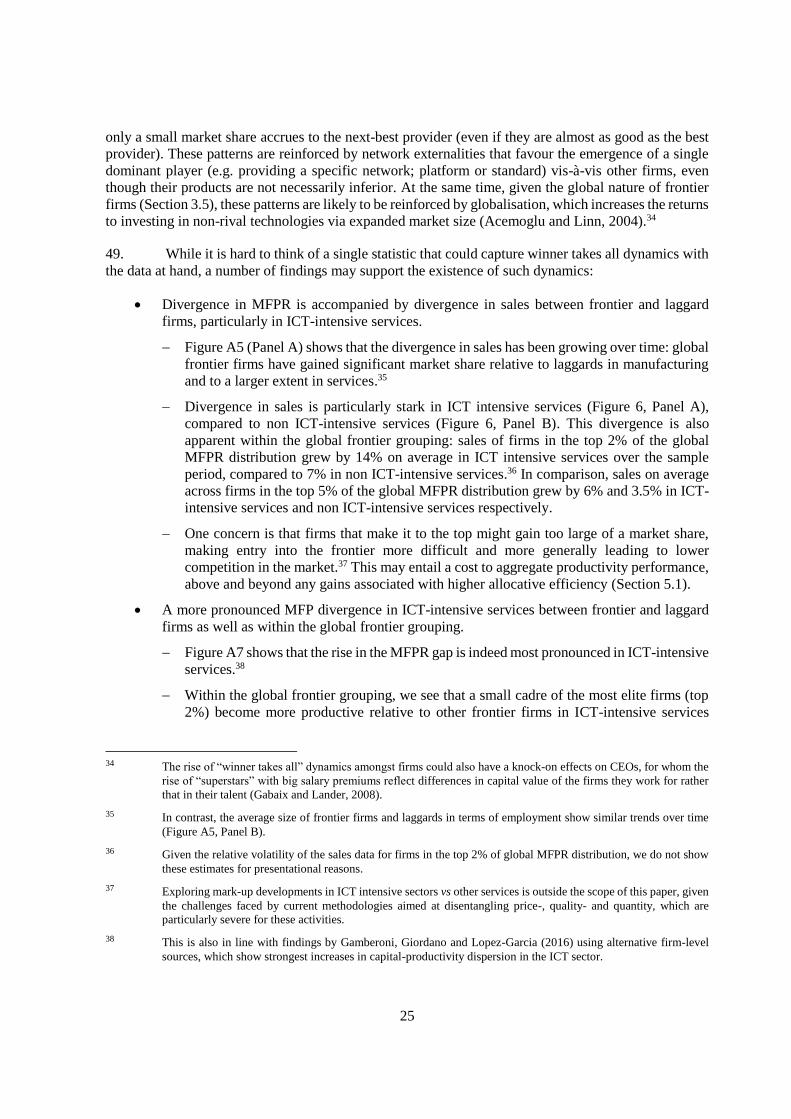
25
only a small market share accrues to the next-best provider (even if they are almost as good as the best
provider). These patterns are reinforced by network externalities that favour the emergence of a single
dominant player (e.g. providing a specific network; platform or standard) vis-à-vis other firms, even
though their products are not necessarily inferior. At the same time, given the global nature of frontier
firms (Section 3.5), these patterns are likely to be reinforced by globalisation, which increases the returns
to investing in non-rival technologies via expanded market size (Acemoglu and Linn, 2004).34
49. While it is hard to think of a single statistic that could capture winner takes all dynamics with
the data at hand, a number of findings may support the existence of such dynamics:
Divergence in MFPR is accompanied by divergence in sales between frontier and laggard
firms, particularly in ICT-intensive services.
Figure A5 (Panel A) shows that the divergence in sales has been growing over time: global
frontier firms have gained significant market share relative to laggards in manufacturing
and to a larger extent in services.35
Divergence in sales is particularly stark in ICT intensive services (Figure 6, Panel A),
compared to non ICT-intensive services (Figure 6, Panel B). This divergence is also
apparent within the global frontier grouping: sales of firms in the top 2% of the global
MFPR distribution grew by 14% on average in ICT intensive services over the sample
period, compared to 7% in non ICT-intensive services.36 In comparison, sales on average
across firms in the top 5% of the global MFPR distribution grew by 6% and 3.5% in ICT-
intensive services and non ICT-intensive services respectively.
One concern is that firms that make it to the top might gain too large of a market share,
making entry into the frontier more difficult and more generally leading to lower
competition in the market.37 This may entail a cost to aggregate productivity performance,
above and beyond any gains associated with higher allocative efficiency (Section 5.1).
A more pronounced MFP divergence in ICT-intensive services between frontier and laggard
firms as well as within the global frontier grouping.
Figure A7 shows that the rise in the MFPR gap is indeed most pronounced in ICT-intensive
services.38
Within the global frontier grouping, we see that a small cadre of the most elite firms (top
2%) become more productive relative to other frontier firms in ICT-intensive services
34 The rise of “winner takes all” dynamics amongst firms could also have a knock-on effects on CEOs, for whom the
rise of “superstars” with big salary premiums reflect differences in capital value of the firms they work for rather
that in their talent (Gabaix and Lander, 2008).
35 In contrast, the average size of frontier firms and laggards in terms of employment show similar trends over time
(Figure A5, Panel B).
36 Given the relative volatility of the sales data for firms in the top 2% of global MFPR distribution, we do not show
these estimates for presentational reasons.
37 Exploring mark-up developments in ICT intensive sectors vs other services is outside the scope of this paper, given
the challenges faced by current methodologies aimed at disentangling price-, quality- and quantity, which are
particularly severe for these activities.
38 This is also in line with findings by Gamberoni, Giordano and Lopez-Garcia (2016) using alternative firm-level
sources, which show strongest increases in capital-productivity dispersion in the ICT sector.
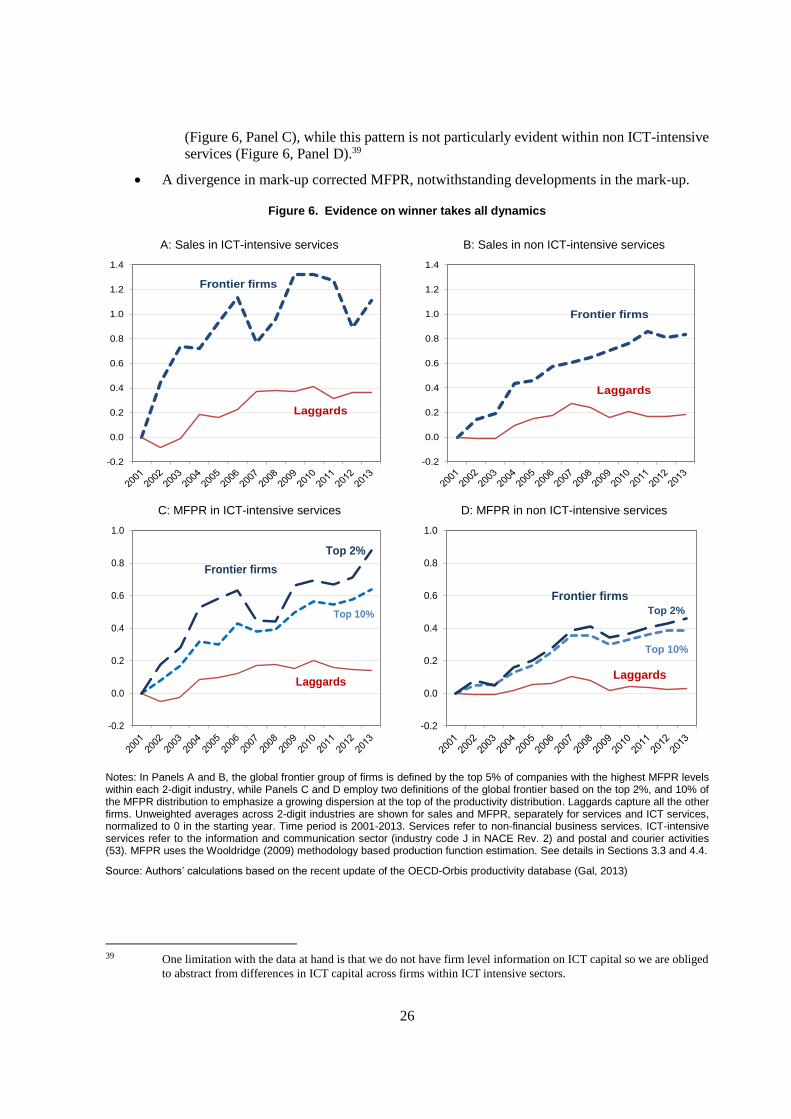
26
(Figure 6, Panel C), while this pattern is not particularly evident within non ICT-intensive
services (Figure 6, Panel D).39
A divergence in mark-up corrected MFPR, notwithstanding developments in the mark-up.
Figure 6. Evidence on winner takes all dynamics
A: Sales in ICT-intensive services
B: Sales in non ICT-intensive services
C: MFPR in ICT-intensive services
D: MFPR in non ICT-intensive services
Notes: In Panels A and B, the global frontier group of firms is defined by the top 5% of companies with the highest MFPR levels within each 2-digit industry, while Panels C and D employ two definitions of the global frontier based on the top 2%, and 10% of the MFPR distribution to emphasize a growing dispersion at the top of the productivity distribution. Laggards capture all the other firms. Unweighted averages across 2-digit industries are shown for sales and MFPR, separately for services and ICT services, normalized to 0 in the starting year. Time period is 2001-2013. Services refer to non-financial business services. ICT-intensive services refer to the information and communication sector (industry code J in NACE Rev. 2) and postal and courier activities (53). MFPR uses the Wooldridge (2009) methodology based production function estimation. See details in Sections 3.3 and 4.4.
Source: Authors’ calculations based on the recent update of the OECD-Orbis productivity database (Gal, 2013)
39 One limitation with the data at hand is that we do not have firm level information on ICT capital so we are obliged
to abstract from differences in ICT capital across firms within ICT intensive sectors.
-0.2
0.0
0.2
0.4
0.6
0.8
1.0
1.2
1.4
Frontier firms
Laggards
-0.2
0.0
0.2
0.4
0.6
0.8
1.0
1.2
1.4
Frontier firms
Laggards
-0.2
0.0
0.2
0.4
0.6
0.8
1.0
Frontier firms
Laggards
Top 10%
Top 2%
-0.2
0.0
0.2
0.4
0.6
0.8
1.0
Frontier firms
Laggards
Top 10%
Top 2%
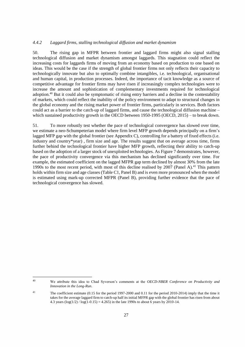
27
4.4.2 Laggard firms, stalling technological diffusion and market dynamism
50. The rising gap in MFPR between frontier and laggard firms might also signal stalling
technological diffusion and market dynamism amongst laggards. This stagnation could reflect the
increasing costs for laggards firms of moving from an economy based on production to one based on
ideas. This would be the case if the strength of global frontier firms not only reflects their capacity to
technologically innovate but also to optimally combine intangibles, i.e. technological, organisational
and human capital, in production processes. Indeed, the importance of tacit knowledge as a source of
competitive advantage for frontier firms may have risen if increasingly complex technologies were to
increase the amount and sophistication of complementary investments required for technological
adoption.40 But it could also be symptomatic of rising entry barriers and a decline in the contestability
of markets, which could reflect the inability of the policy environment to adapt to structural changes in
the global economy and the rising market power of frontier firms, particularly in services. Both factors
could act as a barrier to the catch-up of laggard firms, and cause the technological diffusion machine –
which sustained productivity growth in the OECD between 1950-1995 (OECD, 2015) – to break down.
51. To more robustly test whether the pace of technological convergence has slowed over time,
we estimate a neo-Schumpeterian model where firm level MFP growth depends principally on a firm’s
lagged MFP gap with the global frontier (see Appendix C), controlling for a battery of fixed effects (i.e.
industry and country*year) , firm size and age. The results suggest that on average across time, firms
further behind the technological frontier have higher MFP growth, reflecting their ability to catch-up
based on the adoption of a larger stock of unexploited technologies. As Figure 7 demonstrates, however,
the pace of productivity convergence via this mechanism has declined significantly over time. For
example, the estimated coefficient on the lagged MFPR gap term declined by almost 30% from the late
1990s to the most recent period, with most of this decline realised by 2007 (Panel A).41 This pattern
holds within firm size and age classes (Table C1, Panel B) and is even more pronounced when the model
is estimated using mark-up corrected MFPR (Panel B), providing further evidence that the pace of
technological convergence has slowed.
40 We attribute this idea to Chad Syverson’s comments at the OECD-NBER Conference on Productivity and
Innovation in the Long-Run.
41 The coefficient estimate (0.15 for the period 1997-2000 and 0.11 for the period 2010-2014) imply that the time it
takes for the average laggard firm to catch-up half its initial MFPR gap with the global frontier has risen from about
4.3 years (log(1/2) / log(1-0.15) = 4.265) in the late 1990s to about 6 years by 2010-14.
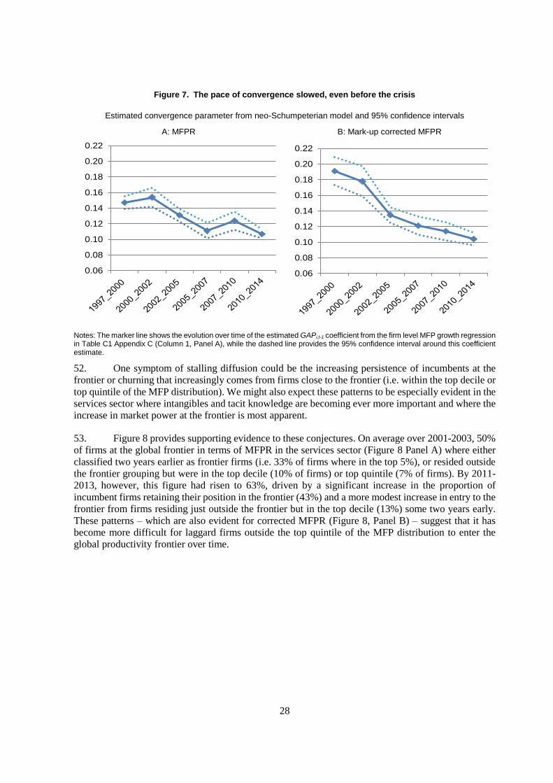
28
Figure 7. The pace of convergence slowed, even before the crisis
Estimated convergence parameter from neo-Schumpeterian model and 95% confidence intervals
A: MFPR
B: Mark-up corrected MFPR
Notes: The marker line shows the evolution over time of the estimated GAPi,t-1 coefficient from the firm level MFP growth regression in Table C1 Appendix C (Column 1, Panel A), while the dashed line provides the 95% confidence interval around this coefficient estimate.
52. One symptom of stalling diffusion could be the increasing persistence of incumbents at the
frontier or churning that increasingly comes from firms close to the frontier (i.e. within the top decile or
top quintile of the MFP distribution). We might also expect these patterns to be especially evident in the
services sector where intangibles and tacit knowledge are becoming ever more important and where the
increase in market power at the frontier is most apparent.
53. Figure 8 provides supporting evidence to these conjectures. On average over 2001-2003, 50%
of firms at the global frontier in terms of MFPR in the services sector (Figure 8 Panel A) where either
classified two years earlier as frontier firms (i.e. 33% of firms where in the top 5%), or resided outside
the frontier grouping but were in the top decile (10% of firms) or top quintile (7% of firms). By 2011-
2013, however, this figure had risen to 63%, driven by a significant increase in the proportion of
incumbent firms retaining their position in the frontier (43%) and a more modest increase in entry to the
frontier from firms residing just outside the frontier but in the top decile (13%) some two years early.
These patterns – which are also evident for corrected MFPR (Figure 8, Panel B) – suggest that it has
become more difficult for laggard firms outside the top quintile of the MFP distribution to enter the
global productivity frontier over time.
0.06
0.08
0.10
0.12
0.14
0.16
0.18
0.20
0.22
0.06
0.08
0.10
0.12
0.14
0.16
0.18
0.20
0.22
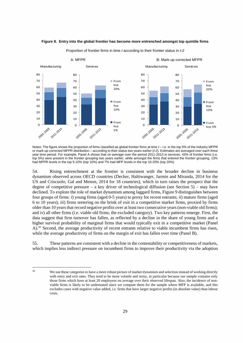
29
Figure 8. Entry into the global frontier has become more entrenched amongst top quintile firms
Proportion of frontier firms in time t according to their frontier status in t-2
A: MFPR
B: Mark-up corrected MFPR
Notes: The figure shows the proportion of firms classified as global frontier firms at time t – i.e. in the top 5% of the industry MFPR or mark-up corrected MFPR distribution – according to their status two years earlier (t-2). Estimates are averaged over each three year time period. For example, Panel A shows that on average over the period 2011-2013 in services, 43% of frontier firms (i.e. top 5%) were present in the frontier grouping two years earlier, while amongst the firms that entered the frontier grouping, 13% had MFPR levels in the top 5-10% (top 10%) and 7% had MFP levels in the top 10-20% (top 20%)
54. Rising entrenchment at the frontier is consistent with the broader decline in business
dynamism observed across OECD countries (Decker, Haltiwanger, Jarmin and Miranda, 2014 for the
US and Criscuolo, Gal and Menon, 2014 for 18 countries), which in turn raises the prospect that the
degree of competitive pressure – a key driver of technological diffusion (see Section 5) – may have
declined. To explore the role of market dynamism among laggard firms, Figure 9 distinguishes between
four groups of firms: i) young firms (aged 0-5 years) to proxy for recent entrants; ii) mature firms (aged
6 to 10 years); iii) firms teetering on the brink of exit in a competitive market firms, proxied by firms
older than 10 years that record negative profits over at least two consecutive years (non-viable old firms);
and iv) all other firms (i.e. viable old firms; the excluded category). Two key patterns emerge. First, the
data suggest that firm turnover has fallen, as reflected by a decline in the share of young firms and a
higher survival probability of marginal firms that would typically exit in a competitive market (Panel
A).42 Second, the average productivity of recent entrants relative to viable incumbent firms has risen,
while the average productivity of firms on the margin of exit has fallen over time (Panel B).
55. These patterns are consistent with a decline in the contestability or competitiveness of markets,
which implies less indirect pressure on incumbent firms to improve their productivity via the adoption
42 We use these categories to have a more robust picture of market dynamism and selection instead of working directly
with entry and exit rates. They tend to be more volatile and noisy, in particular because our sample contains only
those firms which have at least 20 employees on average over their observed lifespan. Also, the incidence of non-
viable firms is likely to be understated since we compute them for the sample where MFP is available, and this
excludes cases with negative value added, i.e. firms that have larger negative profits (in absolute value) than labour
costs.
Manufacturing Services
0
10
20
30
40
50
60
70
80
0
10
20
30
40
50
60
70
80
Fromtop
20%
Fromtop
10%
Fromtop
5%
Manufacturing Services
0
10
20
30
40
50
60
70
80
0
10
20
30
40
50
60
70
80
Fromtop
20%
Fromtop
10%
Fromtop 5%
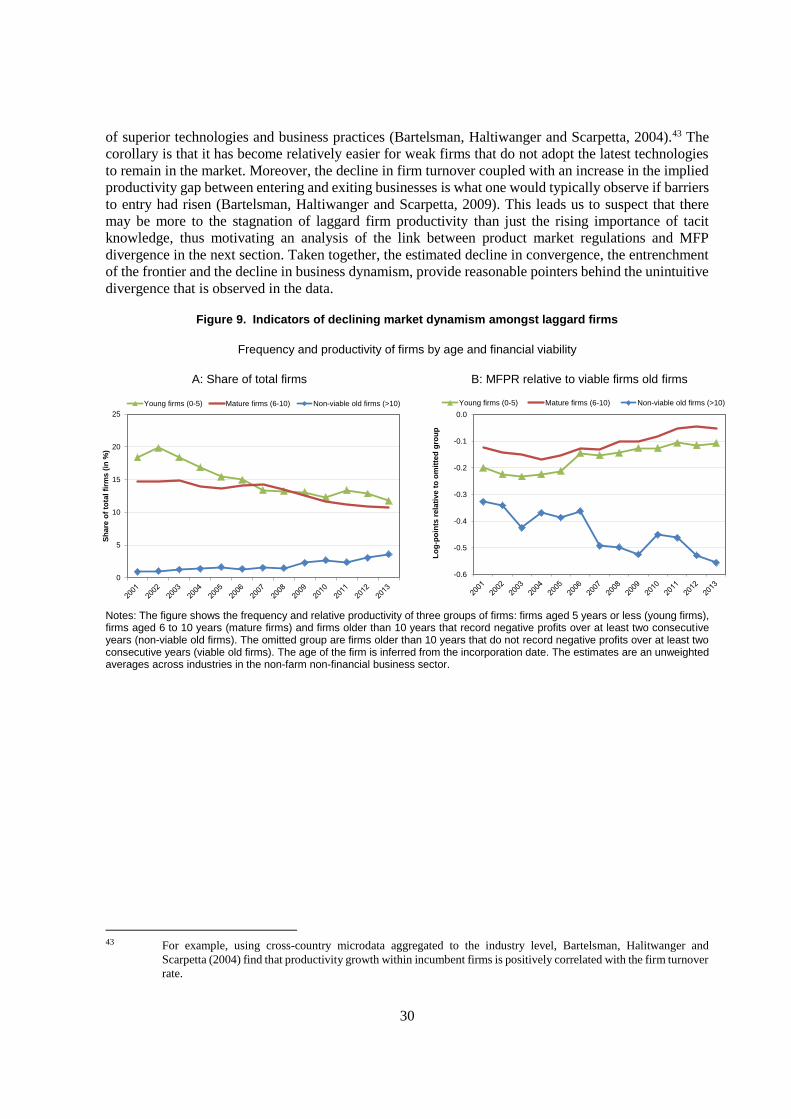
30
of superior technologies and business practices (Bartelsman, Haltiwanger and Scarpetta, 2004).43 The
corollary is that it has become relatively easier for weak firms that do not adopt the latest technologies
to remain in the market. Moreover, the decline in firm turnover coupled with an increase in the implied
productivity gap between entering and exiting businesses is what one would typically observe if barriers
to entry had risen (Bartelsman, Haltiwanger and Scarpetta, 2009). This leads us to suspect that there
may be more to the stagnation of laggard firm productivity than just the rising importance of tacit
knowledge, thus motivating an analysis of the link between product market regulations and MFP
divergence in the next section. Taken together, the estimated decline in convergence, the entrenchment
of the frontier and the decline in business dynamism, provide reasonable pointers behind the unintuitive
divergence that is observed in the data.
Figure 9. Indicators of declining market dynamism amongst laggard firms
Frequency and productivity of firms by age and financial viability
A: Share of total firms
B: MFPR relative to viable firms old firms
Notes: The figure shows the frequency and relative productivity of three groups of firms: firms aged 5 years or less (young firms), firms aged 6 to 10 years (mature firms) and firms older than 10 years that record negative profits over at least two consecutive years (non-viable old firms). The omitted group are firms older than 10 years that do not record negative profits over at least two consecutive years (viable old firms). The age of the firm is inferred from the incorporation date. The estimates are an unweighted averages across industries in the non-farm non-financial business sector.
43 For example, using cross-country microdata aggregated to the industry level, Bartelsman, Halitwanger and
Scarpetta (2004) find that productivity growth within incumbent firms is positively correlated with the firm turnover
rate.
0
5
10
15
20
25
Sh
are
of
tota
l fi
rms
(in
%)
Young firms (0-5) Mature firms (6-10) Non-viable old firms (>10)
-0.6
-0.5
-0.4
-0.3
-0.2
-0.1
0.0
Lo
g-p
oin
ts r
ela
tiv
e t
o o
mit
ted
gro
up
Young firms (0-5) Mature firms (6-10) Non-viable old firms (>10)
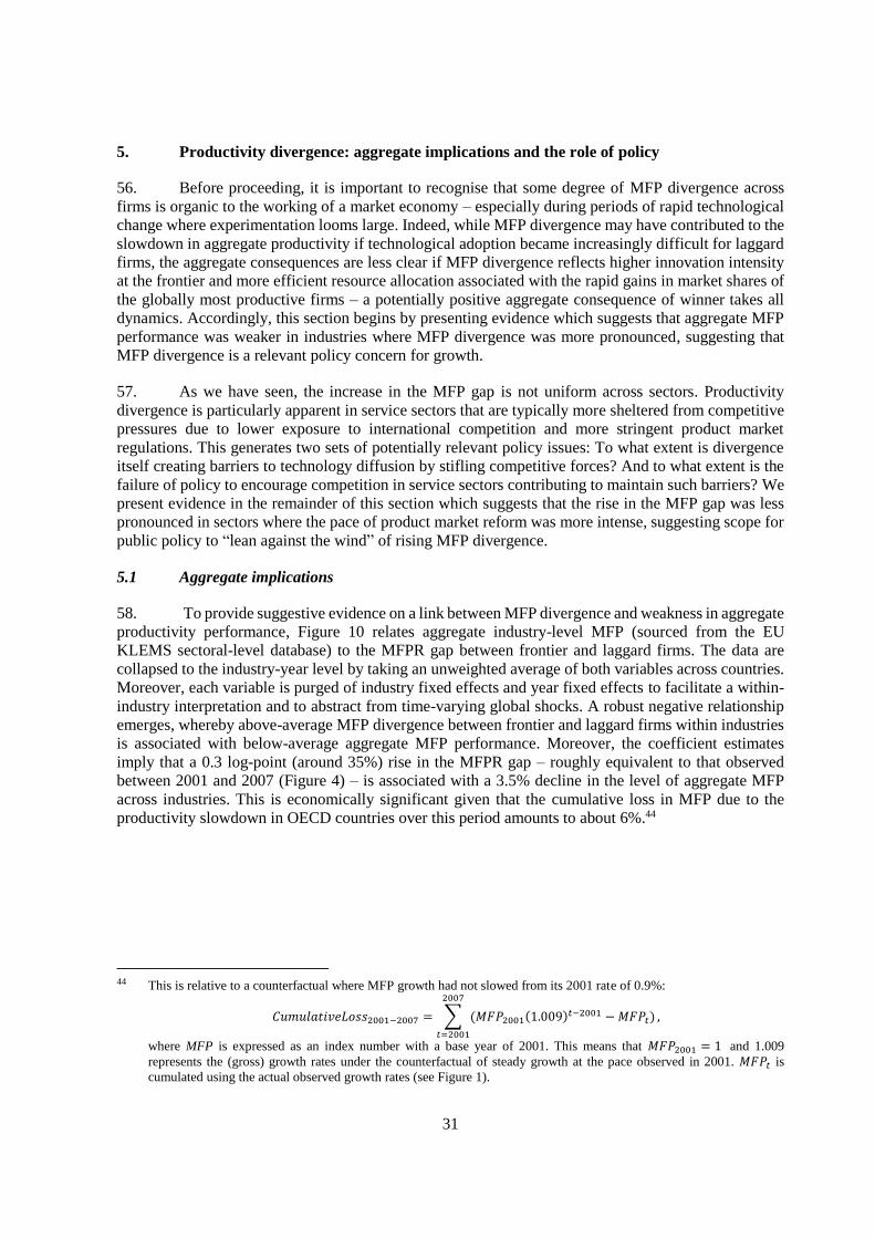
31
5. Productivity divergence: aggregate implications and the role of policy
56. Before proceeding, it is important to recognise that some degree of MFP divergence across
firms is organic to the working of a market economy – especially during periods of rapid technological
change where experimentation looms large. Indeed, while MFP divergence may have contributed to the
slowdown in aggregate productivity if technological adoption became increasingly difficult for laggard
firms, the aggregate consequences are less clear if MFP divergence reflects higher innovation intensity
at the frontier and more efficient resource allocation associated with the rapid gains in market shares of
the globally most productive firms – a potentially positive aggregate consequence of winner takes all
dynamics. Accordingly, this section begins by presenting evidence which suggests that aggregate MFP
performance was weaker in industries where MFP divergence was more pronounced, suggesting that
MFP divergence is a relevant policy concern for growth.
57. As we have seen, the increase in the MFP gap is not uniform across sectors. Productivity
divergence is particularly apparent in service sectors that are typically more sheltered from competitive
pressures due to lower exposure to international competition and more stringent product market
regulations. This generates two sets of potentially relevant policy issues: To what extent is divergence
itself creating barriers to technology diffusion by stifling competitive forces? And to what extent is the
failure of policy to encourage competition in service sectors contributing to maintain such barriers? We
present evidence in the remainder of this section which suggests that the rise in the MFP gap was less
pronounced in sectors where the pace of product market reform was more intense, suggesting scope for
public policy to “lean against the wind” of rising MFP divergence.
5.1 Aggregate implications
58. To provide suggestive evidence on a link between MFP divergence and weakness in aggregate
productivity performance, Figure 10 relates aggregate industry-level MFP (sourced from the EU
KLEMS sectoral-level database) to the MFPR gap between frontier and laggard firms. The data are
collapsed to the industry-year level by taking an unweighted average of both variables across countries.
Moreover, each variable is purged of industry fixed effects and year fixed effects to facilitate a within-
industry interpretation and to abstract from time-varying global shocks. A robust negative relationship
emerges, whereby above-average MFP divergence between frontier and laggard firms within industries
is associated with below-average aggregate MFP performance. Moreover, the coefficient estimates
imply that a 0.3 log-point (around 35%) rise in the MFPR gap – roughly equivalent to that observed
between 2001 and 2007 (Figure 4) – is associated with a 3.5% decline in the level of aggregate MFP
across industries. This is economically significant given that the cumulative loss in MFP due to the
productivity slowdown in OECD countries over this period amounts to about 6%.44
44 This is relative to a counterfactual where MFP growth had not slowed from its 2001 rate of 0.9%:
𝐶𝑢𝑚𝑢𝑙𝑎𝑡𝑖𝑣𝑒𝐿𝑜𝑠𝑠2001−2007 = ∑ (𝑀𝐹𝑃2001(1.009)𝑡−2001 − 𝑀𝐹𝑃𝑡)
2007
𝑡=2001
,
where MFP is expressed as an index number with a base year of 2001. This means that 𝑀𝐹𝑃2001 = 1 and 1.009
represents the (gross) growth rates under the counterfactual of steady growth at the pace observed in 2001. 𝑀𝐹𝑃𝑡 is
cumulated using the actual observed growth rates (see Figure 1).
32
Figure 10. Aggregate MFP performance was weaker in industries where MFPR divergence was greater
Residual aggregate MFP and the MFPR gap at the industry level; 1998-2007
Notes: The figure plots two-digit industry-year observations of aggregate MFP from EU-KLEMS against the MFPR gap (as defined in Figure 2) based on two steps. First, an unweighted average of each variable is computed across 12 OECD countries – Austria, Belgium, Germany, Spain, Finland, France, the United Kingdom, Italy, Japan, the Netherlands, Sweden and the United States – at the industry level for each year between 1998 and 2007. Second, the industry-year observations are purged of two-digit industry fixed effects and year fixed effects. Outlier observations outside the range of 0.4 are removed from the graph. The relationship is statistically significant at the 5% level and is robust to various outlier filtering techniques and to looking within manufacturing or services sectors (see Table D2 of Appendix D).
59. As shown in Table D2 (Panel A) of Appendix D, this negative relationship between aggregate
MFP and MFPR divergence is statistically significant and holds within both manufacturing and
services.45 While this analysis is restricted to the pre-crisis period due to the lack of more recent industry-
level MFP data, a negative relationship is also evident between aggregate labour productivity and labour
productivity divergence over 1998-2013, although this relationship is mainly driven by the
manufacturing sector (see Table D2, Panel B).46 In any case, even with a growing market share accrued
to frontier firms, aggregate productivity is not benefiting positively from a widening gap between the
frontier and laggards. This illustrates that winner takes all dynamics discussed in the previous section
do not necessarily translate into aggregate gains, because they tend to imply poor productivity
performance of laggard firms.
5.2 Productivity divergence and product market regulation
60. At the margin, there are a number of channels through which pro-competitive product market
reforms can strengthen the incentives for laggard firms to adopt frontier technologies, thereby
moderating – but not necessarily reversing – the pressures towards higher MFP divergence induced by
technological change. Indeed, a range of firm-level evidence generally supports the idea that competitive
45 These results are also significant in light of the fact that the aggregate data also reflect the MFP performance of
firms that employ fewer than 20 employees and the changes in allocative efficiency (i.e. resource shifts across firms
within sectors), which we do not account for in our analysis.
46 We also attempted to more directly assess the contribution of the MFP gap to the slowdown in aggregate
productivity growth – i.e. by regressing the change in MFP growth on change in the MFP gap in a long difference
specification – but these attempts were frustrated by the limited availability of reliable industry-level MFP data
over a sufficiently long time span.
33
pressures are a driver of productivity-enhancing innovation and adoption.47 More specifically, pro-
competition reforms in product markets could be expected to promote the catch-up of laggard firms to
the global frontier for a number of reasons:
First, higher competition underpins within-firm productivity gains by weeding out inefficient
firms and sharpening the incentives for incumbent laggard firms to adopt better technologies
and business practices (Bloom, Draca and Van Reenen., 2015; Perla, Tonetti and Waugh,
2015; Steinwender, 2015; Baily, 1993; Baily et al., 2005).
Second, stronger product market competition can improve managerial quality (Bloom and Van
Reenen, 2010), which is complementary to technological adoption (Bloom et al., 2012).
Third, reductions in administrative entry barriers can spur entry, which promotes technological
diffusion to the extent that young firms possess a comparative advantage in commercialising
cutting-edge technologies (Henderson, 1993; Baumol, 2002).
Fourth, pro-competitive reforms to market regulations in upstream services sectors may
increase the returns expected by firms in downstream manufacturing sectors from adopting
best-practice techniques (Bourlès, Cette, Lopez, Mairesse and Nicoletti, 2013).
Finally, product market reforms can promote productivity-enhancing reallocation (Andrews
and Cingano, 2014), thereby enhancing the ability of firms to attract inputs complementary to
technological adoption and achieve sufficient scale to enter global markets and learn from
global frontier firms.
5.3 Product market reforms in OECD countries
61. To measure market reforms, we utilise the OECD database on product market regulations,
which is based on a highly detailed questionnaire sent out to governments every five years (Nicoletti
and Scarpetta, 2003).48 These indicators measure the extent of “anti-competitive” regulations; that is,
regulations “that inhibit competition in markets where competition is viable”.49 A key strength of these
indicators is their de jure nature – i.e. they focus on rules and regulations – which facilitates meaningful
cross-country comparisons, but it is important to note that they do not account for differences in
implementation and enforcement across countries. The indicators range from 0 to 6 and are increasing
in the restrictiveness of product market regulations.
62. We exploit information on sector-specific provisions in 10 separate industries (7 in network
industries, 1 in retail, and 2 in professional services; see Conway and Nicoletti, 2006), as opposed to the
47 See, for instance: Geroski (1995a, 1995b); Nickell (1996); Nickell, Nicolitsas and Dryden (1997); Blundell, Griffith
and Van Reenen, (1999); Griffith, Redding and Simpson (2002); Aghion et al (2004); Haskel, Pereira and Slaughter
(2007).
48 For example, the 2013 questionnaire includes around 1400 questions on economy-wide and sector-specific
provisions (see Koske et al., 2015).
49 As outlined in Nicoletti et al. (2000), the restrictions to competition captured by the OECD indicators of Product
Market Regulation were defined either as barriers to access in markets that are inherently competitive or as
government interferences with market mechanisms in areas in which there are no obvious reasons why such
mechanisms should not be operating freely (e.g. price controls imposed in competitive industries as road freight or
retail distribution). Given that the indicators cover a relatively homogenous set of countries, the underlying
assumption is that regulatory patterns do not reflect cross-country differences in the level of public concern for the
market failures that motivate regulations, but rather reflect regulatory failure or policies adverse to competition.
34
economy-wide indicators.50 As discussed in Gal and Hijzen (2016), regulation in: i) network industries
is largely about the organisation of network access to potential service providers; ii) retail trade typically
takes the form of entry barriers, specific restrictions for large firms and the flexibility of shops in terms
of opening hours and prices; iii) professional services concerns to barriers to entry and the way services
are delivered and includes, amongst others, rules governing the recognition of qualifications and the
determination of fees and prices.
63. According to the OECD indicators, there is considerable scope for further product market
reform in many OECD countries, particularly in market services where the increase in MFP divergence
has been most striking. Within non-manufacturing industries, most reform activity over the past 15 years
has been concentrated in network industries (i.e. energy, transport and communication), and this is
reflected in both a decline in the median level and dispersion of market regulation across countries
(Figure 11, Panel A). While there remains some scope for further reform action in specific network
industries (particularly road and rail transportation) and countries, the need for reforms in retail trade
and professional services is clear. Between 1998 and 2013, the median restrictiveness of product market
regulations only fell modestly in retail (Panel B) and was little changed in professional services (Panel
C), while the dispersion in the restrictiveness of market regulations across countries in these sectors
remains high. If product market regulations affect the incentives for laggard firms to adopt leading
technologies and best practices, to what extent is the rising MFP gap between frontier and laggard firm
in services a product of the slow pace of market reforms in these industries?
50 Network industries include two energy sectors (electricity and gas), three transport sectors (road, rail and air) and
two communication sectors (post and telecommunications). The two professional services industries refer to the
business services sector (accounting and legal services) and the technical services sector (engineering and
architecture services).
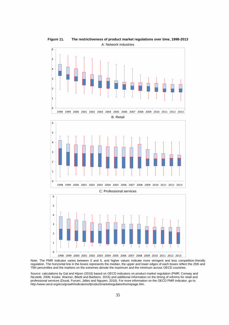
35
Figure 11. The restrictiveness of product market regulations over time, 1998-2013
A: Network industries
B: Retail
C: Professional services
Note: The PMR indicator varies between 0 and 6, and higher values indicate more stringent and less competition-friendly regulation. The horizontal line in the boxes represents the median, the upper and lower edges of each boxes reflect the 25th and 75th percentiles and the markers on the extremes denote the maximum and the minimum across OECD countries.
Source: calculations by Gal and Hijzen (2016) based on OECD indicators on product market regulation (PMR; Conway and Nicoletti, 2006; Koske, Wanner, Bitetti and Barbiero. 2015) and additional information on the timing of reforms for retail and professional services (Duval, Furceri, Jalles and Nguyen, 2016). For more information on the OECD PMR indicator, go to: http://www.oecd.org/eco/growth/indicatorsofproductmarketregulationhomepage.htm.
0
1
2
3
4
5
6
1998 1999 2000 2001 2002 2003 2004 2005 2006 2007 2008 2009 2010 2011 2012 2013
0
1
2
3
4
5
6
1998 1999 2000 2001 2002 2003 2004 2005 2006 2007 2008 2009 2010 2011 2012 2013
0
1
2
3
4
5
6
1998 1999 2000 2001 2002 2003 2004 2005 2006 2007 2008 2009 2010 2011 2012 2013
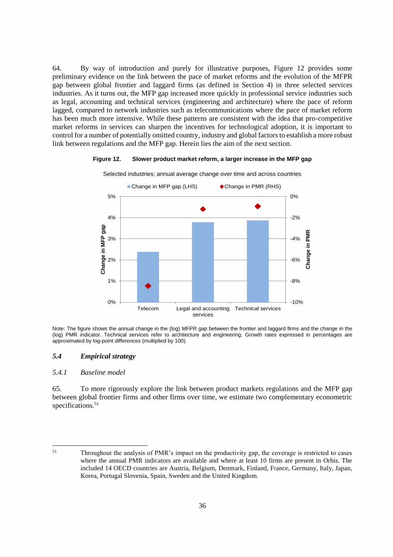
36
64. By way of introduction and purely for illustrative purposes, Figure 12 provides some
preliminary evidence on the link between the pace of market reforms and the evolution of the MFPR
gap between global frontier and laggard firms (as defined in Section 4) in three selected services
industries. As it turns out, the MFP gap increased more quickly in professional service industries such
as legal, accounting and technical services (engineering and architecture) where the pace of reform
lagged, compared to network industries such as telecommunications where the pace of market reform
has been much more intensive. While these patterns are consistent with the idea that pro-competitive
market reforms in services can sharpen the incentives for technological adoption, it is important to
control for a number of potentially omitted country, industry and global factors to establish a more robust
link between regulations and the MFP gap. Herein lies the aim of the next section.
Figure 12. Slower product market reform, a larger increase in the MFP gap
Selected industries; annual average change over time and across countries
Note: The figure shows the annual change in the (log) MFPR gap between the frontier and laggard firms and the change in the (log) PMR indicator. Technical services refer to architecture and engineering. Growth rates expressed in percentages are approximated by log-point differences (multiplied by 100).
5.4 Empirical strategy
5.4.1 Baseline model
65. To more rigorously explore the link between product markets regulations and the MFP gap
between global frontier firms and other firms over time, we estimate two complementary econometric
specifications.51
51 Throughout the analysis of PMR’s impact on the productivity gap, the coverage is restricted to cases
where the annual PMR indicators are available and where at least 10 firms are present in Orbis. The
included 14 OECD countries are Austria, Belgium, Denmark, Finland, France, Germany, Italy, Japan,
Korea, Portugal Slovenia, Spain, Sweden and the United Kingdom.
-10%
-8%
-6%
-4%
-2%
0%
0%
1%
2%
3%
4%
5%
Telecom Legal and accountingservices
Technical servicesC
ha
ng
e i
n P
MR
Ch
an
ge
in
MF
P g
ap
Change in MFP gap (LHS) Change in PMR (RHS)
37
66. First, for 10 market services sectors for which regulatory indicators are available over the
period 1998-2013, we estimate the following long difference specification:
tcstsctcs
ld
tcs
ld
tcs
ld EPMRMFPgap ,,,,2,,10,, [2]
where: Δld denotes the long difference operator, corresponding to five years in the baseline
specification;52 MFPgaps,c,t refers to the difference between the (unweighted) average MFP (MFPR or
mark-up corrected MFPR) of global frontier firms and the (unweighted) average MFP of laggard firms
in country c, industry s and year t; PMRs,c,t refers to the overall restrictiveness of product market
regulation in key service industries (expressed in log terms)53, which is increasing in the degree of
regulation. If β1>0, then it implies that a slowdown in the pace of pro-competitive product market
reforms (i.e. a less negative tcs
ld PMR ,, term) is associated with a rising MFP gap between the global
frontier and non-frontier firms.
67. The regression also includes the growth of sectoral employment (E) to control for time-varying
shocks within country*industry pairings and for changes in the coverage of the dataset over time.54 The
baseline model includes separate country, industry and year fixed effects to control for omitted time-
invariant country (δc) or industry (δs) factors and global shocks (δt), but as an extension, we include
interacted country-year fixed effects (δct) to control for time-varying country-specific shocks. To
maximize the use of the data, we rely on overlapping five-year differences (e.g. 2013-2008, 2012-2007
etc.) but given that we cluster at the country-industry pair level this is innocuous (Bloom et al., 2015).
Finally, country-industry-year cells that contain less than 10 firms are excluded in order to reduce the
influence of highly idiosyncratic firm-level developments.
68. Second, we estimate a dynamic ordinary least squares (see Stock and Watson, 1993; DOLS)
equation in [3], on the same sample of 10 market services sectors over the period 1998-2013. This
specification relates the level of the MFP gap to the (log) level of PMR and lags and leads changes (i.e.
first differences) of the explanatory variables (ΔX) – the latter are included to control for serial
correlation and endogeneity.55 It also includes a rich battery of fixed effects to control for unobserved
time-varying country-specific shocks (δct), time-varying global industry-specific shocks (δst) and time
invariant industry-specific factors within countries (δcs).
tcscsstct
ktkt
j
tcstcstcs tscXEPMRMFPgap ,,
,
,,2,,10,, ,,
[3]
52 As discussed below, the results are not particularly sensitive to the choice of the length of the long difference
window.
53 For retail and professional services industries, where the indicators are updated only every 5 years (1998, 2003,
2008, 2013), additional information was used on the timing of reforms following the calculations of Gal and Hijzen
(2016) and Duval et al (2016). Taking the log of PMR is a useful transformation to the extent that it allows for
reforms to be evaluated in relative terms, in relation to the pre-reform policy stance. This is particularly relevant as
in many industries the level of regulation – as expressed by the PMR indicator – is already at low levels, and there
is limited scope for further reforms that lead to a similar reduction in absolute terms in the indicator than in the
past.
54 The employment variable is based on information from the Orbis database, and is calculated as the average of log
employment levels across firms.
55 DOLS estimates are presented based on both one and two lags and leads.
38
5.4.2 Addressing identification concerns
69. One identification concern is that rigid services regulation might be a consequence, not a cause
of the MFP gap (e.g. reverse causality). This would be the case if in service sectors with many firms
lagging behind the global productivity frontier, there was a greater incentive for firms to exert political
pressures for raising anticompetitive regulations. While such lobby activity by inefficient firms would
upwardly bias the estimate of β1, the tendency for product market reforms to be conducted when
economic conditions are weak (Bouis, Duval and Eugster, 2016) would bias the estimate of β1 in the
opposite direction.
70. We adopt two identification strategies to confront the potential endogeneity of market
regulation to economic conditions and at the industry level. First, we employ an instrument variables
(IV) approach in the context of our long difference framework, which exploits the existence of
liberalization waves across countries and the role of external pressure in driving them (see Bouis et al.,
2016).56 Here, we utilise two instruments which are unlikely to be affected by sector-level economic
outcomes in the country considered, and should not have any effect on MFPgapsct other than through
pressure on domestic authorities to undertake reform:
The lagged level of market regulation, based on the idea that the scope for reform as well as
the push to implement reform is larger the in country-sector pairs where the initial stance of
product market regulation is stricter.
Average reform activity in other countries – as measured by the 5-year change in product
market regulation in the given sector – to capture peer pressure from reforms in other countries.
71. Second, if these baseline estimates are robust, then one might expect there to be a relationship
between the MFP gap in manufacturing sectors and the extent of regulation in upstream service sectors
in those instances where input-output connections are more intense. Accordingly, we estimate a variant
of equation [3] for 22 industries in the manufacturing sector over the period 1998-2013 using the OECD
regulatory impact indicator, which captures the knock-on or indirect effect of product market regulations
in upstream services sectors (Bourlès et al., 2013; Conway and Nicoletti, 2006) on the MFP gap in
downstream manufacturing industries. This is done by crossing the upstream regulatory indicators with
the intensity of use of intermediate inputs calculated from input-output matrices since the impact of
upstream regulations on downstream productivity is an increasing function of the intensity of use of
intermediate inputs from the regulated upstream industries. While political economy factors may again
be a source of bias – for example, if firms in downstream industries that use regulated (upstream)
intermediate inputs, and whose productivity growth is low as a result, were to lobby for and obtain
upstream deregulation – if anything, this would make it more difficult to find a positive relationship
between upstream regulation and the MFP gap in downstream sectors (Bourles et al., 2013).
5.5 Empirical results
5.5.1 Baseline results
72. Table 2, Panel A shows the baseline estimates for the 5-year long difference specification
(Equation 2) for the MFP gap based on MFPR and mark-up corrected MFP for the services sector. The
odd numbered columns include separate country, industry and year fixed effects, while the even
numbered columns include country-year fixed effects – which control for time varying country-specific
shocks – and separate industry fixed effects. In each case, the change in the MFP gap is positively related
56 We employ the IV approach in the context of our baseline long-difference specification since it’s easier to find
plausible instrument variables for reform – i.e. PMR change – then the level of PMR.
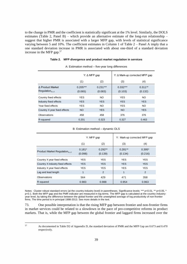
39
to the change in PMR and the coefficient is statistically significant at the 1% level. Similarly, the DOLS
estimates (Table 2, Panel B) – which provide an alternative estimate of the long-run relationship –
suggest that higher PMR is associated with a larger MFP gap, with levels of statistical significance
varying between 5 and 10%. The coefficient estimates in Column 1 of Table 2 – Panel A imply that a
one standard deviation increase in PMR is associated with about one-third of a standard deviation
increase in the MFP gap.57
Table 2. MFP divergence and product market regulation in services
A: Estimation method – five-year long differences
B: Estimation method – dynamic OLS
Notes: Cluster robust standard errors (at the country-industry level) in parentheses. Significance levels: *** p<0.01, ** p<0.05, * p<0.1. Both the MFP gap and the PMR indicator are measured in log terms. The MFP gap is calculated at the country-industry-year level, by taking the difference between the global frontier and the unweighted average of log productivity of non-frontier firms. The time period is in principal 1998-2013. See more details in the text.
73. One possible interpretation is that the rising MFP gap between frontier and non-frontier firms
in market services could be related to a slowdown in the pace of pro-competitive reforms in product
markets. That is, while the MFP gap between the global frontier and laggard firms increased over the
57 As documented in Table D2 of Appendix D, the standard deviation of PMR and the MFP Gap are 0.673 and 0.470
respectively.
(1) (2) (3) (4)
0.205*** 0.231*** 0.332*** 0.311**
(0.065) (0.083) (0.103) (0.132)
Country fixed effects YES NO YES NO
Industry fixed effects YES YES YES YES
Year fixed effects YES NO YES NO
Country X year fixed effects NO YES NO YES
Observations 458 458 376 376
R-squared 0.201 0.323 0.327 0.463
Y: Δ MFP gap Y: Δ Mark-up corrected MFP gap
Δ Product Market
Regulations,c,t
(1) (2) (3) (4)
0.181* 0.292** 0.281** 0.395*
(0.098) (0.139) (0.134) (0.216)
Country X year fixed effects YES YES YES YES
Country X industry fixed effects YES YES YES YES
Industry X year fixed effects YES YES YES YES
Lag and lead length 1 2 1 2
Observations 564 429 471 358
R-squared 0.983 0.988 0.954 0.963
Y: MFP gap Y: Mark-up corrected MFP gap
Product Market Regulations,c,t
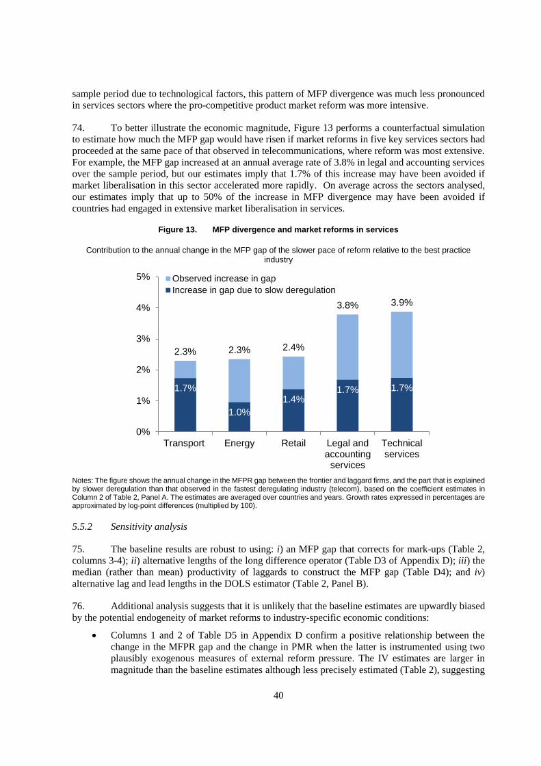
40
sample period due to technological factors, this pattern of MFP divergence was much less pronounced
in services sectors where the pro-competitive product market reform was more intensive.
74. To better illustrate the economic magnitude, Figure 13 performs a counterfactual simulation
to estimate how much the MFP gap would have risen if market reforms in five key services sectors had
proceeded at the same pace of that observed in telecommunications, where reform was most extensive.
For example, the MFP gap increased at an annual average rate of 3.8% in legal and accounting services
over the sample period, but our estimates imply that 1.7% of this increase may have been avoided if
market liberalisation in this sector accelerated more rapidly. On average across the sectors analysed,
our estimates imply that up to 50% of the increase in MFP divergence may have been avoided if
countries had engaged in extensive market liberalisation in services.
Figure 13. MFP divergence and market reforms in services
Contribution to the annual change in the MFP gap of the slower pace of reform relative to the best practice industry
Notes: The figure shows the annual change in the MFPR gap between the frontier and laggard firms, and the part that is explained by slower deregulation than that observed in the fastest deregulating industry (telecom), based on the coefficient estimates in Column 2 of Table 2, Panel A. The estimates are averaged over countries and years. Growth rates expressed in percentages are approximated by log-point differences (multiplied by 100).
5.5.2 Sensitivity analysis
75. The baseline results are robust to using: i) an MFP gap that corrects for mark-ups (Table 2,
columns 3-4); ii) alternative lengths of the long difference operator (Table D3 of Appendix D); iii) the
median (rather than mean) productivity of laggards to construct the MFP gap (Table D4); and iv)
alternative lag and lead lengths in the DOLS estimator (Table 2, Panel B).
76. Additional analysis suggests that it is unlikely that the baseline estimates are upwardly biased
by the potential endogeneity of market reforms to industry-specific economic conditions:
Columns 1 and 2 of Table D5 in Appendix D confirm a positive relationship between the
change in the MFPR gap and the change in PMR when the latter is instrumented using two
plausibly exogenous measures of external reform pressure. The IV estimates are larger in
magnitude than the baseline estimates although less precisely estimated (Table 2), suggesting
2.3% 2.3% 2.4%
3.8% 3.9%
1.7%
1.0%
1.4%1.7% 1.7%
0%
1%
2%
3%
4%
5%
Transport Energy Retail Legal andaccounting
services
Technicalservices
Observed increase in gap
Increase in gap due to slow deregulation
41
that weak sectoral performance may trigger market reforms, as opposed to lobbying for
anticompetitive regulation.
The IV regressions in Table D5 also show a positive relationship between the mark-up
corrected MFPR gap and PMR (Columns 3 and 4), although the imprecise estimation means
that the coefficients are not always statistically significant. That PMR is more strongly related
to MFPR gap than the corrected MFPR gap provides tentative evidence that market reforms
may also operate through decreasing mark-up gaps between frontier and laggards.
We also checked the existence of a relationship between the MFP gap in manufacturing sectors
and the extent of regulation in upstream service sectors in those instances where input-output
connections are more intense. Accordingly, the DOLS estimates in Table D6 of Appendix D
imply that higher PMR in upstream sectors is associated with a larger MFP gap in
manufacturing, and this effect is statistically significant at the 1% level. These results raise the
prospect that aggregate impact of services regulation of the MFP gap is likely to be somewhat
larger than the direct estimates reported in Figure 13.
6. Conclusion and future research
77. In this paper, we aim to contribute to the debate on the global productivity slowdown – which
has by and large been conducted from a macroeconomic perspective – towards a more micro level. We
provide new firm level evidence that highlights the importance of separately considering what happens
to innovation at the frontier as well as the diffusion of technologies to laggards firms. This micro
evidence is both key to motivating new theoretical work and to identifying areas where there may be
more traction for policy reforms to revive productivity growth in OECD countries.
78. The most striking feature of the productivity slowdown is not so much a slowing in the rate of
productivity growth at the global frontier, but rather rising productivity at the global frontier coupled
with an increasing productivity divergence between the global frontier and laggard firms. This
productivity divergence remains after controlling for differences in capital deepening and mark-up
behaviour although there is evidence that market power of frontier firms has increased in services. This
leads us to suspect that the rising MFPR gap between global frontier and laggard firms may in fact
reflect technological divergence.
79. We show that this pattern of MFP divergence, which is at odds with existing models of new-
Schumpeterian growth and of creative destruction, could plausibly reflect the potential for structural
changes in the global economy – namely digitalisation, globalisation and the rising importance of tacit
knowledge – to fuel rapid productivity gains at the global frontier. Yet, aggregate MFP performance
was significantly weaker in industries where MFP divergence was more pronounced, suggesting that
the divergence observed is not solely driven by frontier firm pushing the boundary outward. In this
regard, we contend that increasing MFP divergence – and the global productivity slowdown more
generally – could reflect a slowdown in the technological diffusion process. This stagnation could be a
reflection of increasing costs for laggards firms of moving from an economy based on production to one
based on ideas. But it could also be symptomatic of rising entry barriers and a decline in the
contestability of markets. Crucially, in both cases, there is scope for policy to alleviate the productivity
slowdown.
80. Indeed, we find the rise in MFP divergence to be much more extreme in sectors where pro-
competitive product market reforms were least extensive, suggesting that the observed rise in MFP
divergence might be at least partly due to policy weakness stifling diffusion in OECD economies. A
simple counterfactual exercise suggests that had the pace of product market reforms in retail trade and
professional services been equivalent to that observed in the best practice service sector (i.e.
42
telecommunications), then the extent of MFP divergence may have been up to 50% less than what was
actually observed. Put differently, structural changes in the global economy meant that technological
catch-up to the global productivity frontier became more difficult for the typical firm over the 2000s,
but these difficulties were compounded by policy weakness. From this perspective, the opportunity cost
of poorly designed product market regulations may have risen over time.
81. This research raises a number of issues for future research. First, it would be interesting to
explore the impact of the crisis and macroeconomic policies on global frontier and laggard firms, via
the channels identified in Anzoategui, Coming, Gertler and Martinez (2016) and Gopinath et al (2015).
Second, a logical next step is to connect these findings with other cross-country productivity-related
research at the OECD, which reveals declining business dynamism (Criscuolo et al., 2014), rising
resource misallocation (Berlingieri, Blanchenay and Criscuolo, 2016) and weakening market selection,
particularly the distorting effects on resource reallocation of the rise of “zombie” firms (Adalet
McGowan, Andrews and Millot, 2016). Third, policies that can contain MFP divergence may carry a
double-dividend for inclusiveness to the extent that the observed rise in wage inequality is closely related
to the rising dispersion in average wages paid across firms (Card, Heining and Kline, 2013; Song et al.,
2016).
82. The results of this analysis also suggest scope for policy relevant research in other areas. For
example, to the extent that technological adoption is complementary to investments in organisational
capital (Bloom, Sadun and Van Reenen, 2012), it would be interesting to explore the link between
managerial quality and technological divergence. The same is true for IPR regimes given their intuitive
link with winner take all dynamics and opportunities for technological diffusion, although nuanced
cross-country policy indicators of IPRs are currently lacking. Finally, given the increasing potential for
entrenchment at the frontier, concerns about non-technological barriers to entry – such as lobbying
activity by incumbents to prevent the proliferation of new business models and regulatory incumbency
more generally– represent a fruitful area for future research.
43
REFERENCES
Acemoglu, D., P. Aghion and F. Zilibotti (2006), “Distance to the Frontier, Selection and Economic
Growth”, Journal of the European Economic Association 4(1), pp. 37-74.
Acemoglu, D. and J. Linn (2004), “Market Size in Innovation: Theory and Evidence from the
Pharmaceutical Industry”, The Quarterly Journal of Economics, 119, issue 3, p. 1049-1090.
Ackerberg, D., Caves, K., and Frazer, G. (2015), “Identification properties of recent production function
estimators”, Econometrica, Forthcoming.
Aghion, Philippe, and Peter Howitt. 1992. “A Model of Growth Through Creative Destruction."
Econometrica 60, no. 2: 323-351.
Aghion, Philippe, Richard Blundell, Rachel Griffith, Peter Howitt, and Susanne Prantl (2004), ‘‘Entry
and Productivity Growth: Evidence from Micro level Panel Data,’’ Journal of the European
Economic Association 2 (2004), 265–276.
Adalet McGowan, M., D. Andrews and V. Millot (2016), “The Walking Dead? Zombie Firms and
Productivity Performance in OECD countries”, OECD Economics Department Working Paper
forthcoming.
Aghion, P. and P. Howitt (1998), Endogenous Growth Theory, MIT Press.
Aghion, P. and P. Howitt (2006), “Appropriate Growth Policy: A Unifying Framework” Journal of the
European Economic Association 4(2-3), pp. 269-314.
Ahmad, N. and P. Schreyer (2016), "Measuring GDP in a Digitalised Economy", OECD Statistics
Working Papers, No. 2016/07, OECD Publishing, Paris.
DOI: http://dx.doi.org/10.1787/5jlwqd81d09r-en
Andrews, D. and F. Cingano (2014), “Public Policy and Resource Allocation: Evidence from firms in
OECD countries” Economic Policy, Issue 74 April.
Andrews, D., C. Criscuolo and P. Gal (2015), “Frontier firms, technology diffusion and public policy:
micro evidence from OECD countries”, OECD Productivity Working Papers No. 2.
Anzoategui, D., D. Comin, M. Gertler and J. Martinez (2015), "Endogenous Technology Adoption and
R&D as Sources of Business Cycle Persistence". NBER Working Paper No. 22005.
Baily, M. N. (1993), “Competition, Regulation, and Efficiency in Service Industries”, Brookings Papers
on Economic Activity, 1993, No. 2
Baily, M. N., D. Farrell, E. Greenberg, J-D. Henrich, N. Jinjo, M. Jolles, J. Remes (2005), “Increasing
Global Competition and Labor Productivity: Lessons from the US Automotive Industry”,
McKinsey Global Institute, McKinsey & Company, November 2005
Bartelsman, E.J. and M. Doms (2000), “Understanding Productivity: Lessons from Longitudinal
Microdata”, Journal of Economic Literature 38(3), pp. 569-594.
Bartelsman, E., J. Haltiwanger and S. Scarpetta (2013). "Cross-Country Differences in Productivity:
The Role of Allocation and Selection," American Economic Review, 103(1): 305-34.
Baumol, W.J. (2002), The Free-Market Innovation Machine: Analyzing the Growth Miracle of
Capitalism Princeton University Press.
44
Berlingieri, G, P. Blanchaney and C. Criscuolo (2016), “The Great Divergence(s)” OECD Science,
Technology and Innovation Working Paper forthcoming.
Bertrand, M., E. Duflo and S. Mullainathan (2004), “How Much Should We Trust Differences in
Differences Estimates”, Quarterly Journal of Economics, Vol. 119(1), pp. 249-275.
Bourlès, R., G. Cette, J. Lopez, J. Mairesse and G. Nicoletti (2013), "Do Product Market Regulations in
Upstream Sectors Curb Productivity Growth?: Panel Data Evidence for OECD Countries",
Review of Economics and Statistics, 95(5), pp. 1750-1768.
Bloom, N. and J. Van Reenen (2007), “Measuring and Explaining Management Practices Across Firms
and Countries”, Quarterly Journal of Economics, 122 (4), pp. 1351-1408.
Bloom, N., M. Draca and J. Van Reenen (2015), “Trade Induced Technical Change? The Impact of
Chinese Imports on Innovation, IT and Productivity”, Review of Economic Studies, 83(1), pages
87-117.
Bloom, N., R. Sadun and J. Van Reenen (2012a), “Americans Do IT Better: US Multinationals and the
Productivity Miracle”, American Economic Review, 102(1): 167–201.
Blundell, Richard, Rachel Griffith, and John Van Reenen (1999), ‘‘Market Share, Market Value and
Innovation in a Panel of British Manufacturing Firms,’’ Review of Economic Studies 66, pp. 529–
554.
Bouis, R., R. Duval and J. Eugster (2016), “Product Market Deregulation and Growth: New Country-
Industry-Level Evidence,” IMF Working Paper WP/16/114.
Bourlès, R., et al. (2013), “Do Product Market Regulations in Upstream Sectors Curb Productivity
Growth?: Panel Data Evidence for OECD Countries”, The Review of Economics and Statistics,
Vol. 95(5), pp. 1750-1768.
Brynjolfsson, E, and A. McAfee (2011), Race Against The Machine: How the Digital Revolution is
Accelerating Innovation, Driving Productivity, and Irreversibly Transforming Employment and
the Economy, Digital Frontier Press.
Byrne, D. and C. A. Corrado (2015), “Prices for Communications Equipment: Rewriting the Record,”
Finance and Economics Discussion Series 2015-069. Washington: Board of Governors of the
Federal Reserve System, http://dx.doi.org/10.17016/FEDS.2015.069.
Byrne, D., J. Fernald and M. Reinsdorf (2016), “Does the United States have a productivity slowdown
or a measurement problem?” Brookings Papers on Economic Activity Conference Draft, March
10-11, 2016
Caballero, R. J and M. L. Hammour (1994) "The Cleansing Effect of Recessions," American Economic
Review, vol. 84(5), pages 1350-68, December.
Campbell, J. (1998), Entry, Exit, Embodied Technology, and Business Cycles, Review of Economic
Dynamics, 1, (2), 371-408
Card, D., J. Heining and P. Kline (2013), “Workplace Heterogeneity and the Rise of West German Wage
Inequality”, Quarterly Journal of Economics, 128(3), pp. 967-1015.
Christiano, L.J., M.S. Eichenbaum and M. Trabandt (2015), “Understanding the Great Recession”,
American Economic Journal: Macroeconomics 7(1): 110–167
45
Comin, D and M. Mestieri (2013), “If Technology Has Arrived Everywhere, Why Has Income
Diverged?” NBER Working Paper Series, No. 19010.
Conway, P. and G. Nicoletti, 2006, "Product Market Regulation in the Non-Manufacturing Sectors of
OECD Countries: Measurement and Highlights", OECD Economics Department Working
Papers, No. 530, OECD Publishing, Paris.
Cooper, R., J. Haltiwanger and L. Power (1997). “Machine replacement and the business cycle: lumps
and bumps.” NBER Working Paper No. 5260.
Corrado, C., C. Hulten and D. Sichel (2009), "Intangible Capital And U.S. Economic Growth," Review
of Income and Wealth, International Association for Research in Income and Wealth, vol. 55(3),
pages 661-685, 09.
Cowen, T. (2011), The Great Stagnation: How America Ate All the Low-Hanging Fruit of Modern
History, Got Sick, and Will (Eventually) Feel Better.
Criscuolo, C, P. Gal, C. Menon (2014), “The Dynamics of Employment Growth: New Evidence from
17 Countries” OECD STI Policy Papers No. 14.
David, P. A. (1991), "Computer and Dynamo: The Modern Productivity Paradox in a Not‐Too‐Distant
Mirror," in Technology and Productivity: The Challenge for Economic Policy, Organization for
Economic Co‐operation and Development, Paris, pp. 315‐48.
Decker, R., J. Haltiwanger, R.S. Jarmin, and J. Miranda (2014), “The role of entrepreneurship in U.S.
job creation and economic dynamism”, Journal of Economic Perspectives (28), pp. 3-24.
Decker, R., J. Haltiwanger, R.S. Jarmin, and J. Miranda (2016), “Where Has All the Skewness Gone?
The Decline in High-Growth (Young) Firms in the U.S”, European Economic Review 86 (July):
4-23.
De Loecker, J. and J. v. Biesebroeck, 2016, “Effect of International Competition on Firm Productivity
and Market Power”, NBER Working Paper No. 21994.
De Loecker, J. and F. Warzynski, 2012. “Mark-ups and Firm-Level Export Status”, American Economic
Review Vol. 102, No. 6, October 2012 (pp. 2437-71)
Derviş K. and Z. Qureshi, 2016, “The Productivity Slump – fact or fiction: the measurement debate”,
brief, the Brookings Institution, Washington D.C.
Dunning, J.H. (1981), International Production and the Multinational Enterprise George, Allen, and
Unwin, London.
Duval, R., D. Furceri, J. Jalles, and H. Nguyen, 2016, “A New Narrative Database of Product and Labour
Market Reforms in Advanced Economies.” IMF Working Paper, forthcoming.
Fernald, J. (2014), “Productivity and Potential Output Before, During, and After the Great Recession”,
in: NBER Macroeconomics Annual 2014, Volume 29.
Forlani, E., R. Martin, G. Mion and M. Muûls (2016), “Unraveling Firms: Demand, Productivity and
Mark-ups Heterogeneity”, EP Discussion Paper No 1402.
Foster, L., J. Haltiwanger and C. J. Krizan (2001) “Aggregate Productivity Growth: Lessons from
Microeconomic Evidence.” In New Developments in Productivity Analysis, Edward Dean,
Michael Harper, and Charles Hulten, eds. Chicago: University of Chicago Press, 303-372.
46
Foster, L., J. Haltiwanger and C. Syverson (2008), “Reallocation, Firm Turnover, and Efficiency:
Selection on Productivity or Profitability?,” American Economic Review 98(1), pages 394-42.
Gal, P. (2013), “Measuring Total Factor Productivity at the Firm Level using OECD-ORBIS”, OECD
Economics Department Working Papers No. 1049, OECD, Paris.
Gal, P. and A. Hijzen (2016), “The short-term impact of product market reforms: A cross-country firm-
level analysis”, OECD Economics Department Working Paper No. 1311.
Geroski, P (1995a), ‘‘What Do We Know about Entry?’’ International Journal of Industrial
Organization 13, 421–440.
Geroski, P (1995b), Market Structure, Corporate Performance and Innovative Activity (Oxford: Oxford
University Press).
Gopinath, G., S. Kalemli-Ozcan, L. Karabarbounis and C. Villegas-Sanchez (2015), “Capital Allocation
and Productivity in South Europe”, NBER Working Paper No. 21453Forlani, E., R. Martin, G.
Mion and M. Muuls. 2016 “Unraveling Firms: Demand, Productivity and Mark-ups
Heterogeneity” CEP Discussion Paper No 1402
Gordon, R. (2012), “Is U.S. Economic Growth Over? Faltering Innovation Confronts the Six
Headwinds”, NBER Working Papers, No. 18315.
Griffith, R., S. Redding, and H. Simpson (2002), ‘‘Productivity Convergence and Foreign Ownership at
the Establishment level,’’ CEPR discussion paper 3765 (2002).
Griffith, R., S. Redding and H. Simpson (2006), "Technological Catch-Up and the Role of
Multinationals", Revised Version of CEPR Discussion Paper No. 3765.
Griliches, Z. (1957), “Hybrid Corn: An Exploration in the Economics of Technological Change”
Econometrica vol. 25 (October).
Hall, R. E. (1986), “Market structure and macroeconomic fluctuations”, Brookings Papers on Economic
Activity, 2:285–338.
Haltiwanger, J. (2016), “Firm Dynamics and Productivity: TFPQ, TFPR and Demand Side Factors”,
Economia (forthcoming)
Haskel, J., S. Pereira, and M. Slaughter (2007), ‘‘Does Inward Foreign Direct Investment Boost the
Productivity of Domestic Firms?’’ The Review of Economics and Statistics 89:3, 482–496.
Henderson, R. (1993), “Underinvestment and Incompetence as Responses to Radical Innovation:
Evidence from the Photolithographic Alignment Equipment Industry”, RAND Journal of
Economics 24(2), pp. 248–270.
Hsieh, C-T. and P. Klenow (2009), "Misallocation and Manufacturing Productivity in China and India,"
Quarterly Journal of Economics, 124(4), pp. 1403-1448.
Hulten, C. (2001) "Total Factor Productivity: A Short Biography," in New Developments
in Productivity Analysis, Charles R. Hulten, Edwin R. Dean, and Michael J. Harper, eds., Studies
in Income and Wealth, vol. 63, The University of Chicago Press for the National Bureau of
Economic Research, Chicago, 2001, 1-47.
Inklaar, R and M.P. Timmer, 2014. "The Relative Price of Services," Review of Income and Wealth,
International Association for Research in Income and Wealth, vol. 60(4), pages 727-746,
December.
47
Jones, B. F. (2012), "The Burden of Knowledge and the 'Death of the Renaissance Man': Is Innovation
Getting Harder?", Review of Economic Studies, Vol. 76, pp. 283-317.
Jovanovic, B and G. MacDonald (1994), “Competitive Diffusion”, Journal of Political Economy 102(1),
pp. 24-52.
Jovanovic, B. and P.L. Rousseau (2005), “General Purpose Technologies”, in: P. Aghion and S. Durlauf
(ed.), Handbook of Economic Growth, edition 1, volume 1, chapter 18, pages 1181-1224 Elsevier.
Kalemli-Ozcan, S., B. Sorensen, C. Villegas-Sanchez, V. Volosovych and S. Yesiltas, 2015, "How to
Construct Nationally Representative Firm Level data from the Orbis Global Database," NBER
Working Papers 21558, National Bureau of Economic Research, Inc.
Koske, I., I. Wanner, R. Bitetti and O. Barbiero, 2015, “The 2013 update of the OECD's database on
product market regulation: Policy insights for OECD and non-OECD countries”, OECD
Economics Department Working Papers, No. 1200, OECD Publishing.
Levinsohn, James and Amil Petrin (2003) “Estimating Production Functions Using Inputs to Control for
Unobservables,” Review of Economic Studies, Vol. 70, No. 2, pp. 317–341.
Melitz, M. (2003), “The Impact of Trade on Intra-Industry Reallocations and Aggregate Industry
Productivity”, Econometrica, Vol. 71, pp. 1695-1725.
Mokyr, J (2014), “The Next Age of Invention: Technology’s future is brighter than pessimists allow”,
in Brian C. Anderson ed., City Journal, Manhattan Institute, Winter 2014, pp. 14-20.
Moulton, B.R. (1991), “An Illustration of a Pitfall in Estimating the Effects of Aggregate Variables on
Micro Units”, Review of Economics and Statistics, Vol. 72, pp. 334-338.
Nickell, Stephen, ‘‘Competition and Corporate Performance,’’ Journal of Political Economy 104
(1996), 724–746.
Nickell, S., Daphne´ Nicolitsas, and Neil Dryden, ‘‘What Makes Firms Perform Well?’’ European
Economic Review 41 (1997), 783–796.
Nicoletti, G., S. Scarpetta and O. Boylaud (2000). ‘Summary indicators of product market regulation
with an extension to employment protection legislation’, OECD Economics Department Working
Papers 226, Paris.
OECD. (2013), Addressing Base Erosion and Profit Shifting, OECD Publishing, Paris.DOI:
http://dx.doi.org/10.1787/9789264192744-en
OECD (2015), The Future of Productivity, OECD Publishing, Paris.
OECD (2016), Economic Outlook, Volume 2016, Issue 1, OECD Publishing, Paris.
Perla, J., C. Tonetti and M. Waugh (2015), “Equilibrium Technology Diffusion, Trade and Growth”,
NBER Working Papers, No. 20881.
Petrin, A. and J. Levinsohn (2012),“Measuring aggregate productivity growth using plant-level data”
The RAND Journal of Economics, Volume 43, Issue 4, pages 705–725, Winter 2012
Ribeiro, P. S., S. Menghinello and K. De Backer (2010), "The OECD Orbis Database: Responding to
the Need for Firm-Level Micro-Data in the OECD", OECD Statistics Working Papers, No.
2010/01, OECD Publishing, Paris.
48
Song, J., D. J. Price, F. Guvenen, N. Bloom and T. von Wachter (2015), “Firming up Inequality”, NBER
Working Papers, No. 21199.
Steinwender, C (2015), “The Roles of Import Competition and Export Opportunities for Technical
Change”, CEP Discussion Paper No 1334.
Stock, J., & Watson, M. (1993), “A Simple Estimator of Cointegrating Vectors in Higher Order
Integrated Systems”, Econometrica, 61(4), 783-820.
Summers, L (2016), “The Age of Secular Stagnation: What It Is and What to Do About It,” Foreign
Affairs March/April issue.
Syverson, C. (2004), "Product Substitutability and Productivity Dispersion," Review of Economics and
Statistics, May 2004
Syverson, C (2016), “Challenges to Mismeasurement Explanations for the U.S. Productivity
Slowdown”, NBER Working Paper No. 21974.
Wooldridge, J. M., 2009,“On estimating firm-level production functions using proxy variables to control
for unobservables,” Economics Letters, Vol. 104.
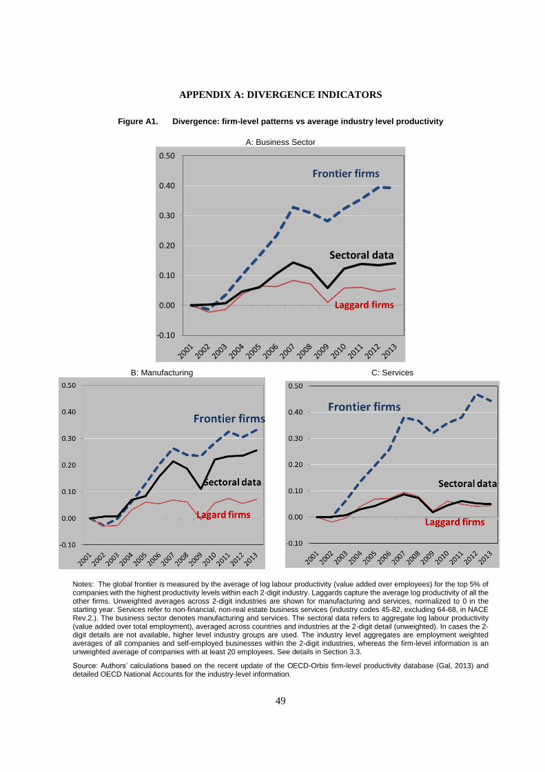
49
APPENDIX A: DIVERGENCE INDICATORS
Figure A1. Divergence: firm-level patterns vs average industry level productivity
A: Business Sector
B: Manufacturing
C: Services
Notes: The global frontier is measured by the average of log labour productivity (value added over employees) for the top 5% of companies with the highest productivity levels within each 2-digit industry. Laggards capture the average log productivity of all the other firms. Unweighted averages across 2-digit industries are shown for manufacturing and services, normalized to 0 in the starting year. Services refer to non-financial, non-real estate business services (industry codes 45-82, excluding 64-68, in NACE Rev.2.). The business sector denotes manufacturing and services. The sectoral data refers to aggregate log labour productivity (value added over total employment), averaged across countries and industries at the 2-digit detail (unweighted). In cases the 2-digit details are not available, higher level industry groups are used. The industry level aggregates are employment weighted averages of all companies and self-employed businesses within the 2-digit industries, whereas the firm-level information is an unweighted average of companies with at least 20 employees. See details in Section 3.3.
Source: Authors’ calculations based on the recent update of the OECD-Orbis firm-level productivity database (Gal, 2013) and detailed OECD National Accounts for the industry-level information.
-0.10
0.00
0.10
0.20
0.30
0.40
0.50
Frontier firms
Laggard firms
Sectoral data
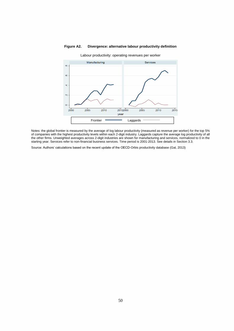
50
Figure A2. Divergence: alternative labour productivity definition
Labour productivity: operating revenues per worker
Notes: the global frontier is measured by the average of log labour productivity (measured as revenue per worker) for the top 5% of companies with the highest productivity levels within each 2-digit industry. Laggards capture the average log productivity of all the other firms. Unweighted averages across 2-digit industries are shown for manufacturing and services, normalized to 0 in the starting year. Services refer to non-financial business services. Time period is 2001-2013. See details in Section 3.3.
Source: Authors’ calculations based on the recent update of the OECD-Orbis productivity database (Gal, 2013)
Frontier Laggards
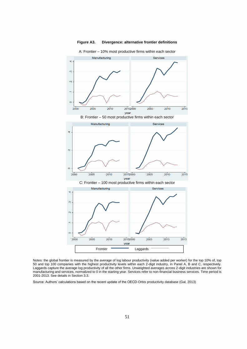
51
Figure A3. Divergence: alternative frontier definitions
A: Frontier – 10% most productive firms within each sector
B: Frontier – 50 most productive firms within each sector
C: Frontier – 100 most productive firms within each sector
Notes: the global frontier is measured by the average of log labour productivity (value added per worker) for the top 10% of, top 50 and top 100 companies with the highest productivity levels within each 2-digit industry, in Panel A, B and C, respectively. Laggards capture the average log productivity of all the other firms. Unweighted averages across 2-digit industries are shown for manufacturing and services, normalized to 0 in the starting year. Services refer to non-financial business services. Time period is 2001-2013. See details in Section 3.3.
Source: Authors’ calculations based on the recent update of the OECD-Orbis productivity database (Gal, 2013)
Frontier Laggards
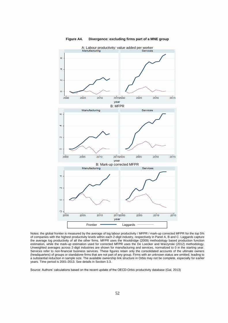
52
Figure A4. Divergence: excluding firms part of a MNE group
A: Labour productivity: value added per worker
B: MFPR
B: Mark-up corrected MFPR
Notes: the global frontier is measured by the average of log labour productivity / MFPR / mark-up corrected MFPR for the top 5% of companies with the highest productivity levels within each 2-digit industry, respectively in Panel A, B and C. Laggards capture the average log productivity of all the other firms. MFPR uses the Wooldridge (2009) methodology based production function estimation, while the mark-up estimation used for corrected MFPR uses the De Loecker and Warzynski (2012) methodology. Unweighted averages across 2-digit industries are shown for manufacturing and services, normalized to 0 in the starting year. Services refer to non-financial business services. These figures retain only the consolidated accounts of the ultimate owners (headquarters) of groups or standalone firms that are not part of any group. Firms with an unknown status are omitted, leading to a substantial reduction in sample size. The available ownership link structure in Orbis may not be complete, especially for earlier years. Time period is 2001-2013. See details in Section 3.3.
Source: Authors’ calculations based on the recent update of the OECD-Orbis productivity database (Gal, 2013)
Frontier Laggards
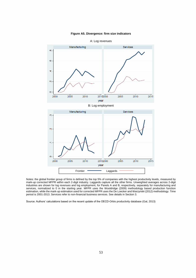
53
Figure A5. Divergence: firm size indicators
A: Log revenues
B: Log employment
Notes: the global frontier group of firms is defined by the top 5% of companies with the highest productivity levels, measured by mark-up corrected MFPR within each 2-digit industry. Laggards capture all the other firms. Unweighted averages across 2-digit industries are shown for log revenues and log employment, for Panels A and B, respectively, separately for manufacturing and services, normalized to 0 in the starting year. MFPR uses the Wooldridge (2009) methodology based production function estimation, while the mark-up estimation used for corrected MFPR uses the De Loecker and Warzynski (2012) methodology. Time period is 2001-2013. Services refer to non-financial business services. See details in Section 3.
Source: Authors’ calculations based on the recent update of the OECD-Orbis productivity database (Gal, 2013)
Frontier Laggards
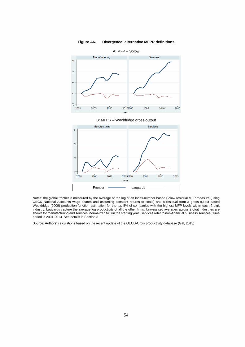
54
Figure A6. Divergence: alternative MFPR definitions
A: MFP – Solow
B: MFPR – Wooldridge gross-output
Notes: the global frontier is measured by the average of the log of an index-number based Solow residual MFP measure (using OECD National Accounts wage shares and assuming constant returns to scale) and a residual from a gross-output based Wooldridge (2009) production function estimation for the top 5% of companies with the highest MFP levels within each 2-digit industry. Laggards capture the average log productivity of all the other firms. Unweighted averages across 2-digit industries are shown for manufacturing and services, normalized to 0 in the starting year. Services refer to non-financial business services. Time period is 2001-2013. See details in Section 3.
Source: Authors’ calculations based on the recent update of the OECD-Orbis productivity database (Gal, 2013)
Frontier Laggards
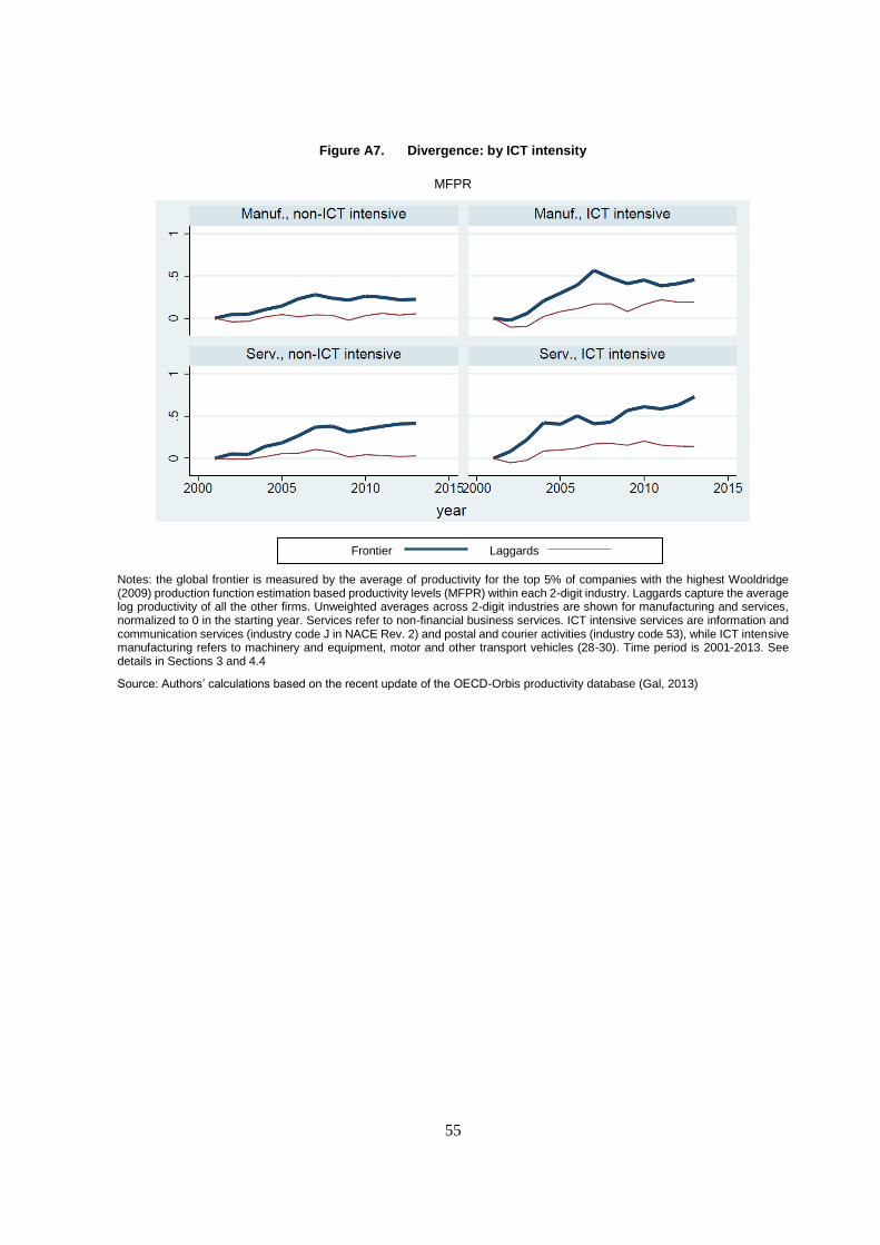
55
Figure A7. Divergence: by ICT intensity
MFPR
Notes: the global frontier is measured by the average of productivity for the top 5% of companies with the highest Wooldridge (2009) production function estimation based productivity levels (MFPR) within each 2-digit industry. Laggards capture the average log productivity of all the other firms. Unweighted averages across 2-digit industries are shown for manufacturing and services, normalized to 0 in the starting year. Services refer to non-financial business services. ICT intensive services are information and communication services (industry code J in NACE Rev. 2) and postal and courier activities (industry code 53), while ICT intensive manufacturing refers to machinery and equipment, motor and other transport vehicles (28-30). Time period is 2001-2013. See details in Sections 3 and 4.4
Source: Authors’ calculations based on the recent update of the OECD-Orbis productivity database (Gal, 2013)
Frontier Laggards
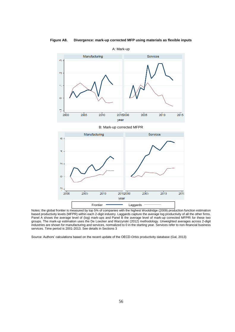
56
Figure A8. Divergence: mark-up corrected MFP using materials as flexible inputs
A: Mark-up
B: Mark-up corrected MFPR
Notes: the global frontier is measured by top 5% of companies with the highest Wooldridge (2009) production function estimation based productivity levels (MFPR) within each 2-digit industry. Laggards capture the average log productivity of all the other firms. Panel A shows the average level of (log) mark-ups and Panel B the average level of mark-up corrected MFPR\ for these two groups. The mark-up estimation uses the De Loecker and Warzynski (2012) methodology. Unweighted averages across 2-digit industries are shown for manufacturing and services, normalized to 0 in the starting year. Services refer to non-financial business services. Time period is 2001-2013. See details in Sections 3
Source: Authors’ calculations based on the recent update of the OECD-Orbis productivity database (Gal, 2013)
Frontier Laggards
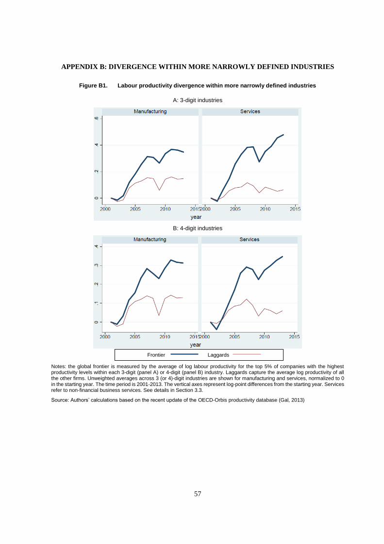
57
APPENDIX B: DIVERGENCE WITHIN MORE NARROWLY DEFINED INDUSTRIES
Figure B1. Labour productivity divergence within more narrowly defined industries
A: 3-digit industries
B: 4-digit industries
Notes: the global frontier is measured by the average of log labour productivity for the top 5% of companies with the highest productivity levels within each 3-digit (panel A) or 4-digit (panel B) industry. Laggards capture the average log productivity of all the other firms. Unweighted averages across 3 (or 4)-digit industries are shown for manufacturing and services, normalized to 0 in the starting year. The time period is 2001-2013. The vertical axes represent log-point differences from the starting year. Services refer to non-financial business services. See details in Section 3.3.
Source: Authors’ calculations based on the recent update of the OECD-Orbis productivity database (Gal, 2013)
Frontier Laggards
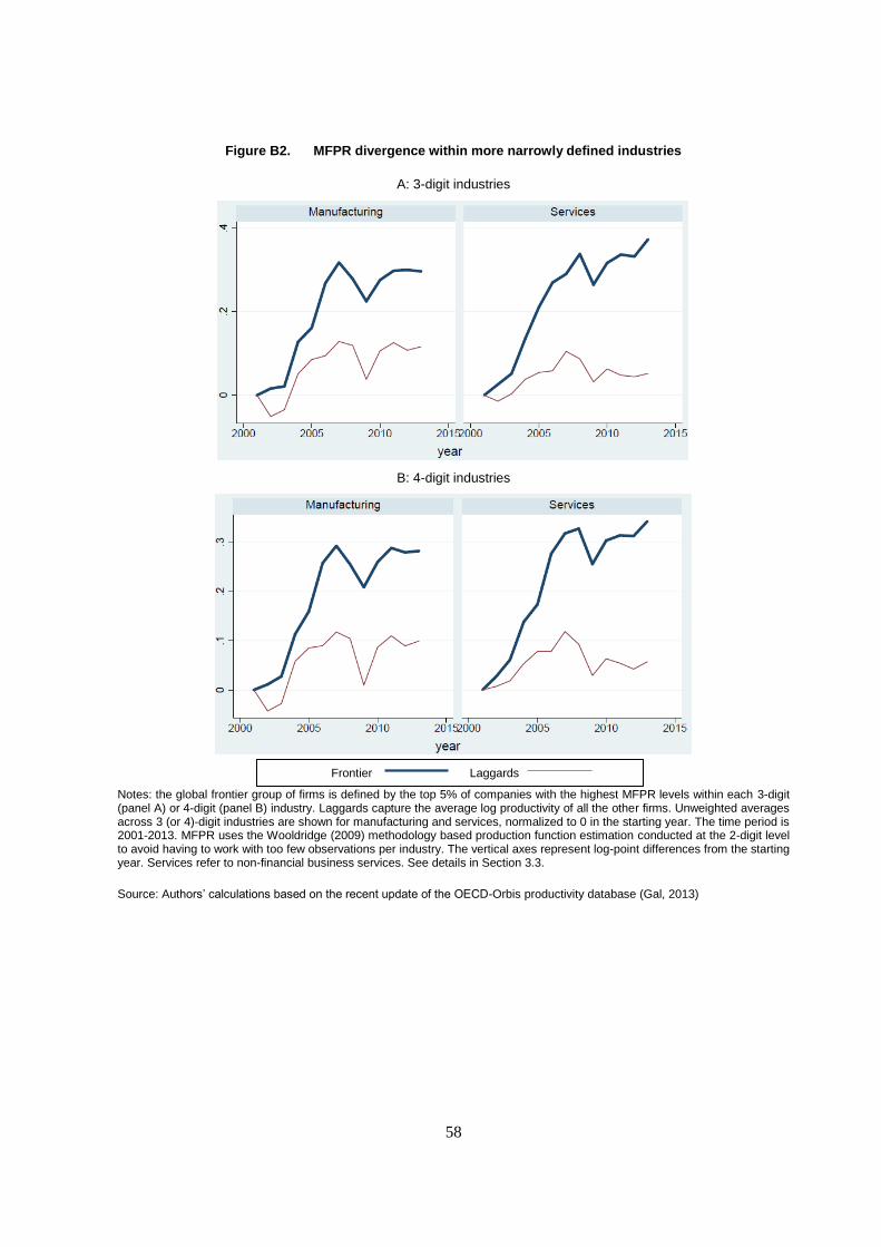
58
Figure B2. MFPR divergence within more narrowly defined industries
A: 3-digit industries
B: 4-digit industries
Notes: the global frontier group of firms is defined by the top 5% of companies with the highest MFPR levels within each 3-digit (panel A) or 4-digit (panel B) industry. Laggards capture the average log productivity of all the other firms. Unweighted averages across 3 (or 4)-digit industries are shown for manufacturing and services, normalized to 0 in the starting year. The time period is 2001-2013. MFPR uses the Wooldridge (2009) methodology based production function estimation conducted at the 2-digit level to avoid having to work with too few observations per industry. The vertical axes represent log-point differences from the starting year. Services refer to non-financial business services. See details in Section 3.3.
Source: Authors’ calculations based on the recent update of the OECD-Orbis productivity database (Gal, 2013)
Frontier Laggards
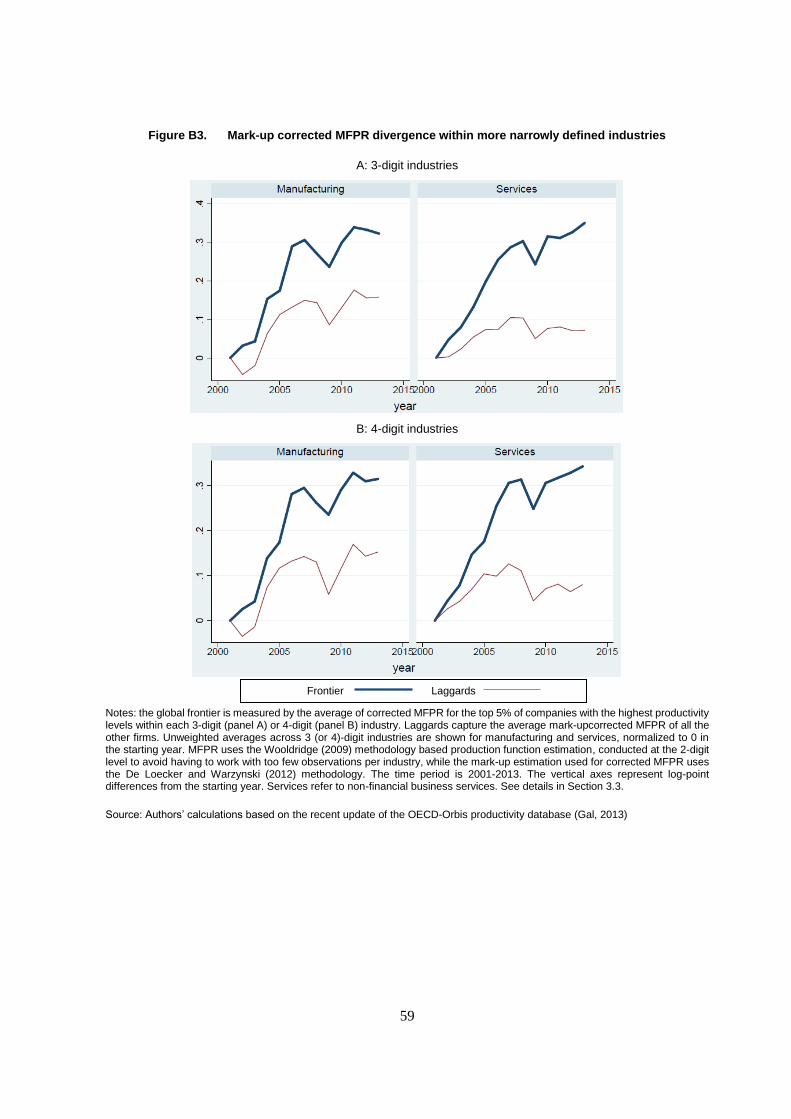
59
Figure B3. Mark-up corrected MFPR divergence within more narrowly defined industries
A: 3-digit industries
B: 4-digit industries
Notes: the global frontier is measured by the average of corrected MFPR for the top 5% of companies with the highest productivity levels within each 3-digit (panel A) or 4-digit (panel B) industry. Laggards capture the average mark-upcorrected MFPR of all the other firms. Unweighted averages across 3 (or 4)-digit industries are shown for manufacturing and services, normalized to 0 in the starting year. MFPR uses the Wooldridge (2009) methodology based production function estimation, conducted at the 2-digit level to avoid having to work with too few observations per industry, while the mark-up estimation used for corrected MFPR uses the De Loecker and Warzynski (2012) methodology. The time period is 2001-2013. The vertical axes represent log-point differences from the starting year. Services refer to non-financial business services. See details in Section 3.3.
Source: Authors’ calculations based on the recent update of the OECD-Orbis productivity database (Gal, 2013)
Frontier Laggards
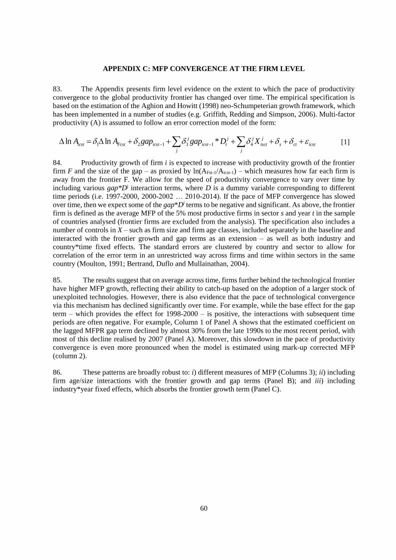
60
APPENDIX C: MFP CONVERGENCE AT THE FIRM LEVEL
83. The Appendix presents firm level evidence on the extent to which the pace of productivity
convergence to the global productivity frontier has changed over time. The empirical specification is
based on the estimation of the Aghion and Howitt (1998) neo-Schumpeterian growth framework, which
has been implemented in a number of studies (e.g. Griffith, Redding and Simpson, 2006). Multi-factor
productivity (A) is assumed to follow an error correction model of the form:
icstcts
j
isct
j
jj
ticst
j
j
icstFcsticst XDgapgapAA 413121 *lnln [1]
84. Productivity growth of firm i is expected to increase with productivity growth of the frontier
firm F and the size of the gap – as proxied by ln(AFst-1/Aicst-1) – which measures how far each firm is
away from the frontier F. We allow for the speed of productivity convergence to vary over time by
including various gap*Dj interaction terms, where D is a dummy variable corresponding to different
time periods (i.e. 1997-2000, 2000-2002 … 2010-2014). If the pace of MFP convergence has slowed
over time, then we expect some of the gap*Dj terms to be negative and significant. As above, the frontier
firm is defined as the average MFP of the 5% most productive firms in sector s and year t in the sample
of countries analysed (frontier firms are excluded from the analysis). The specification also includes a
number of controls in X – such as firm size and firm age classes, included separately in the baseline and
interacted with the frontier growth and gap terms as an extension – as well as both industry and
country*time fixed effects. The standard errors are clustered by country and sector to allow for
correlation of the error term in an unrestricted way across firms and time within sectors in the same
country (Moulton, 1991; Bertrand, Duflo and Mullainathan, 2004).
85. The results suggest that on average across time, firms further behind the technological frontier
have higher MFP growth, reflecting their ability to catch-up based on the adoption of a larger stock of
unexploited technologies. However, there is also evidence that the pace of technological convergence
via this mechanism has declined significantly over time. For example, while the base effect for the gap
term – which provides the effect for 1998-2000 – is positive, the interactions with subsequent time
periods are often negative. For example, Column 1 of Panel A shows that the estimated coefficient on
the lagged MFPR gap term declined by almost 30% from the late 1990s to the most recent period, with
most of this decline realised by 2007 (Panel A). Moreover, this slowdown in the pace of productivity
convergence is even more pronounced when the model is estimated using mark-up corrected MFP
(column 2).
86. These patterns are broadly robust to: i) different measures of MFP (Columns 3); ii) including
firm age/size interactions with the frontier growth and gap terms (Panel B); and iii) including
industry*year fixed effects, which absorbs the frontier growth term (Panel C).
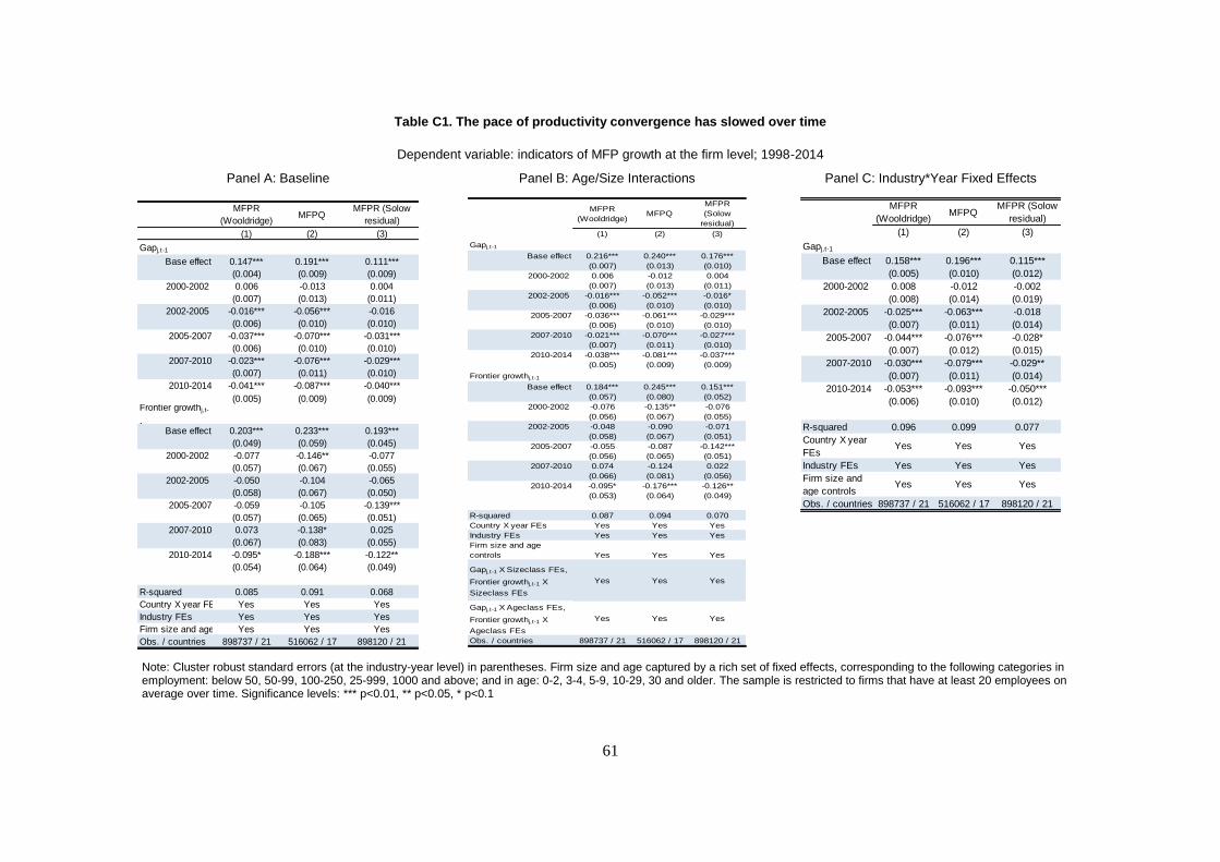
61
Table C1. The pace of productivity convergence has slowed over time
Dependent variable: indicators of MFP growth at the firm level; 1998-2014
Panel A: Baseline
Panel B: Age/Size Interactions
Panel C: Industry*Year Fixed Effects
Note: Cluster robust standard errors (at the industry-year level) in parentheses. Firm size and age captured by a rich set of fixed effects, corresponding to the following categories in employment: below 50, 50-99, 100-250, 25-999, 1000 and above; and in age: 0-2, 3-4, 5-9, 10-29, 30 and older. The sample is restricted to firms that have at least 20 employees on average over time. Significance levels: *** p<0.01, ** p<0.05, * p<0.1
MFPR
(Wooldridge)MFPQ
MFPR (Solow
residual)
(1) (2) (3)
Gapj,t-1
Base effect 0.147*** 0.191*** 0.111***
(0.004) (0.009) (0.009)
0.006 -0.013 0.004
(0.007) (0.013) (0.011)
2002-2005 -0.016*** -0.056*** -0.016
(0.006) (0.010) (0.010)
2005-2007 -0.037*** -0.070*** -0.031***
(0.006) (0.010) (0.010)
2007-2010 -0.023*** -0.076*** -0.029***
(0.007) (0.011) (0.010)
2010-2014 -0.041*** -0.087*** -0.040***
(0.005) (0.009) (0.009)Frontier growthj,t-
1Base effect 0.203*** 0.233*** 0.193***
(0.049) (0.059) (0.045)
-0.077 -0.146** -0.077
(0.057) (0.067) (0.055)
2002-2005 -0.050 -0.104 -0.065
(0.058) (0.067) (0.050)
2005-2007 -0.059 -0.105 -0.139***
(0.057) (0.065) (0.051)
2007-2010 0.073 -0.138* 0.025
(0.067) (0.083) (0.055)
2010-2014 -0.095* -0.188*** -0.122**
(0.054) (0.064) (0.049)
R-squared 0.085 0.091 0.068
Country X year FEs Yes Yes Yes
Industry FEs Yes Yes Yes
Firm size and age controlsYes Yes Yes
Obs. / countries 898737 / 21 516062 / 17 898120 / 21
2000-2002
2000-2002
MFPR
(Wooldridge)MFPQ
MFPR
(Solow
residual)
(1) (2) (3)
Gapj,t-1
Base effect 0.216*** 0.240*** 0.176***
(0.007) (0.013) (0.010)
0.006 -0.012 0.004
(0.007) (0.013) (0.011)
2002-2005 -0.016*** -0.052*** -0.016*
(0.006) (0.010) (0.010)
2005-2007 -0.036*** -0.061*** -0.029***
(0.006) (0.010) (0.010)
2007-2010 -0.021*** -0.070*** -0.027***
(0.007) (0.011) (0.010)
2010-2014 -0.038*** -0.081*** -0.037***
(0.005) (0.009) (0.009)
Frontier growthj,t-1
Base effect 0.184*** 0.245*** 0.151***
(0.057) (0.080) (0.052)
-0.076 -0.135** -0.076
(0.056) (0.067) (0.055)
2002-2005 -0.048 -0.090 -0.071
(0.058) (0.067) (0.051)
2005-2007 -0.055 -0.087 -0.142***
(0.056) (0.065) (0.051)
2007-2010 0.074 -0.124 0.022
(0.066) (0.081) (0.056)
2010-2014 -0.095* -0.176*** -0.126**
(0.053) (0.064) (0.049)
R-squared 0.087 0.094 0.070
Country X year FEs Yes Yes Yes
Industry FEs Yes Yes Yes
Firm size and age
controls Yes Yes Yes
Gapj,t-1 X Sizeclass FEs,
Frontier growthj,t-1 X
Sizeclass FEs
Yes Yes Yes
Gapj,t-1 X Ageclass FEs,
Frontier growthj,t-1 X
Ageclass FEs
Yes Yes Yes
Obs. / countries 898737 / 21 516062 / 17 898120 / 21
2000-2002
2000-2002
MFPR
(Wooldridge)MFPQ
MFPR (Solow
residual)
(1) (2) (3)
Gapj,t-1
Base effect 0.158*** 0.196*** 0.115***
(0.005) (0.010) (0.012)
0.008 -0.012 -0.002
(0.008) (0.014) (0.019)
2002-2005 -0.025*** -0.063*** -0.018
(0.007) (0.011) (0.014)
2005-2007 -0.044*** -0.076*** -0.028*
(0.007) (0.012) (0.015)
2007-2010 -0.030*** -0.079*** -0.029**
(0.007) (0.011) (0.014)
2010-2014 -0.053*** -0.093*** -0.050***
(0.006) (0.010) (0.012)
R-squared 0.096 0.099 0.077
Country X year
FEsYes Yes Yes
Industry FEs Yes Yes Yes
Firm size and
age controlsYes Yes Yes
Obs. / countries 898737 / 21 516062 / 17 898120 / 21
2000-2002
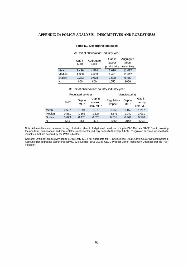
62
APPENDIX D: POLICY ANALYSIS – DESCRIPTIVES AND ROBUSTNESS
Table D1. Descriptive statistics
A: Unit of observation: industry-year
B: Unit of observation: country-industry-year
Note: All variables are measured in logs. Industry refers to 2-digit level detail according to ISIC Rev. 4 / NACE Rev 2, covering the non-farm, non-financial and non-rental business sector (industry codes 5-82 except 64-68). *Regulated services include those industries that are covered by the PMR indicator.
Sources: Orbis (for productivity gaps); EU KLEMS ISIC4 (for aggregate MFP, 12 countries, 1998-2007); OECD Detailed National Accounts (for aggregate labour productivity, 22 countries, 1998-2013); OECD Product Market Regulation Database (for the PMR indicator).
Gap in
MFP
Aggregate
MFP
Gap in
labour
productivity
Aggregate
labour
productivity
Mean 1.426 4.584 1.618 11.687
Median 1.368 4.603 1.421 11.612
St.dev. 0.383 0.078 0.698 0.482
N 600 600 1056 1056
PMRGap in
MFP
Gap in
markup
corr. MFP
Regulatory
Impact
Gap in
MFP
Gap in
markup
corr. MFP
Mean 0.607 1.294 1.272 -3.658 1.152 1.217
Median 0.811 1.163 1.127 -3.571 1.040 1.031
St.dev. 0.673 0.470 0.523 0.551 0.464 0.570
N 564 564 471 2042 2042 1703
Regulated services* Manufacturing
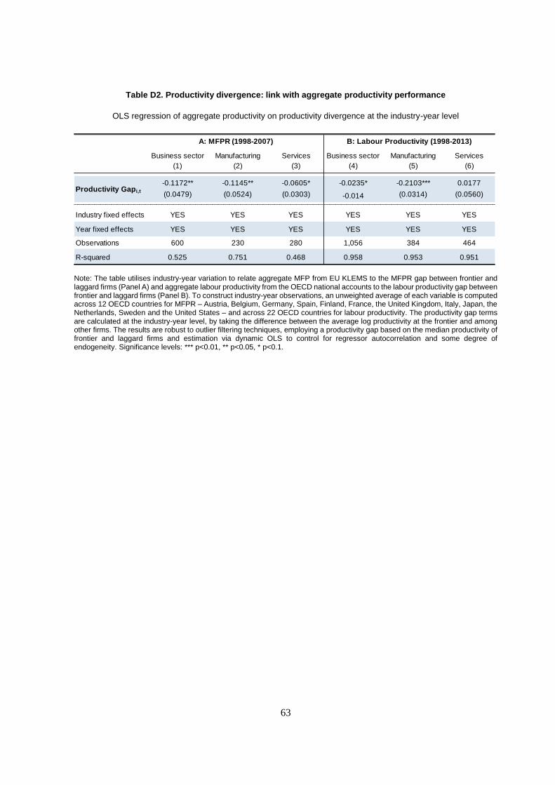
63
Table D2. Productivity divergence: link with aggregate productivity performance
OLS regression of aggregate productivity on productivity divergence at the industry-year level
Note: The table utilises industry-year variation to relate aggregate MFP from EU KLEMS to the MFPR gap between frontier and laggard firms (Panel A) and aggregate labour productivity from the OECD national accounts to the labour productivity gap between frontier and laggard firms (Panel B). To construct industry-year observations, an unweighted average of each variable is computed across 12 OECD countries for MFPR – Austria, Belgium, Germany, Spain, Finland, France, the United Kingdom, Italy, Japan, the Netherlands, Sweden and the United States – and across 22 OECD countries for labour productivity. The productivity gap terms are calculated at the industry-year level, by taking the difference between the average log productivity at the frontier and among other firms. The results are robust to outlier filtering techniques, employing a productivity gap based on the median productivity of frontier and laggard firms and estimation via dynamic OLS to control for regressor autocorrelation and some degree of endogeneity. Significance levels: *** p<0.01, ** p<0.05, * p<0.1.
Business sector Manufacturing Services Business sector Manufacturing Services
(1) (2) (3) (4) (5) (6)
-0.1172** -0.1145** -0.0605* -0.0235* -0.2103*** 0.0177
(0.0479) (0.0524) (0.0303) -0.014 (0.0314) (0.0560)
Industry fixed effects YES YES YES YES YES YES
Year fixed effects YES YES YES YES YES YES
Observations 600 230 280 1,056 384 464
R-squared 0.525 0.751 0.468 0.958 0.953 0.951
A: MFPR (1998-2007) B: Labour Productivity (1998-2013)
Productivity Gapi,t
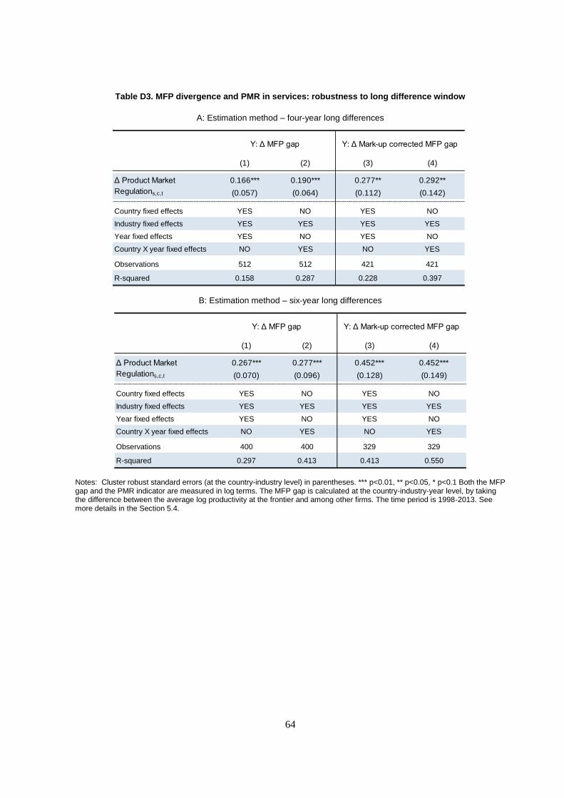
64
Table D3. MFP divergence and PMR in services: robustness to long difference window
A: Estimation method – four-year long differences
B: Estimation method – six-year long differences
Notes: Cluster robust standard errors (at the country-industry level) in parentheses. *** p<0.01, ** p<0.05, * p<0.1 Both the MFP gap and the PMR indicator are measured in log terms. The MFP gap is calculated at the country-industry-year level, by taking the difference between the average log productivity at the frontier and among other firms. The time period is 1998-2013. See more details in the Section 5.4.
(1) (2) (3) (4)
0.166*** 0.190*** 0.277** 0.292**
(0.057) (0.064) (0.112) (0.142)
Country fixed effects YES NO YES NO
Industry fixed effects YES YES YES YES
Year fixed effects YES NO YES NO
Country X year fixed effects NO YES NO YES
Observations 512 512 421 421
R-squared 0.158 0.287 0.228 0.397
Y: Δ MFP gap Y: Δ Mark-up corrected MFP gap
Δ Product Market
Regulations,c,t
(1) (2) (3) (4)
0.267*** 0.277*** 0.452*** 0.452***
(0.070) (0.096) (0.128) (0.149)
Country fixed effects YES NO YES NO
Industry fixed effects YES YES YES YES
Year fixed effects YES NO YES NO
Country X year fixed effects NO YES NO YES
Observations 400 400 329 329
R-squared 0.297 0.413 0.413 0.550
Y: Δ MFP gap Y: Δ Mark-up corrected MFP gap
Δ Product Market
Regulations,c,t
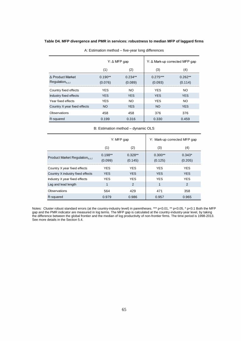
65
Table D4. MFP divergence and PMR in services: robustness to median MFP of laggard firms
A: Estimation method – five-year long differences
B: Estimation method – dynamic OLS
Notes: Cluster robust standard errors (at the country-industry level) in parentheses. *** p<0.01, ** p<0.05, * p<0.1 Both the MFP gap and the PMR indicator are measured in log terms. The MFP gap is calculated at the country-industry-year level, by taking the difference between the global frontier and the median of log productivity of non-frontier firms. The time period is 1998-2013. See more details in the Section 5.4.
(1) (2) (3) (4)
0.190** 0.234** 0.275*** 0.262**
(0.076) (0.089) (0.093) (0.114)
Country fixed effects YES NO YES NO
Industry fixed effects YES YES YES YES
Year fixed effects YES NO YES NO
Country X year fixed effects NO YES NO YES
Observations 458 458 376 376
R-squared 0.199 0.316 0.330 0.459
Y: Δ MFP gap Y: Δ Mark-up corrected MFP gap
Δ Product Market
Regulations,c,t
(1) (2) (3) (4)
0.198** 0.328** 0.300** 0.343*
(0.099) (0.145) (0.125) (0.205)
Country X year fixed effects YES YES YES YES
Country X industry fixed effects YES YES YES YES
Industry X year fixed effects YES YES YES YES
Lag and lead length 1 2 1 2
Observations 564 429 471 358
R-squared 0.979 0.986 0.957 0.965
Y: MFP gap Y: Mark-up corrected MFP gap
Product Market Regulations,c,t
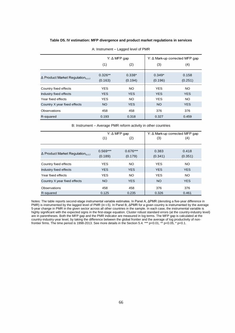
66
Table D5. IV estimation: MFP divergence and product market regulations in services
A: Instrument – Lagged level of PMR
B: Instrument – Average PMR reform activity in other countries
Notes: The table reports second-stage instrumental variable estimates. In Panel A, ΔPMR (denoting a five-year difference in PMR) is instrumented by the lagged level of PMR (in t-5). In Panel B, ΔPMR for a given country is instrumented by the average 5-year change in PMR in the given sector across all other countries in the sample. In each case, the instrumental variable is highly significant with the expected signs in the first-stage equation. Cluster robust standard errors (at the country-industry level) are in parentheses. Both the MFP gap and the PMR indicator are measured in log terms. The MFP gap is calculated at the country-industry-year level, by taking the difference between the global frontier and the average of log productivity of non-frontier firms. The time period is 1998-2013. See more details in the Section 5.4. *** p<0.01, ** p<0.05, * p<0.1.
(1) (2) (3) (4)
0.326** 0.338* 0.349* 0.158
(0.163) (0.194) (0.196) (0.251)
Country fixed effects YES NO YES NO
Industry fixed effects YES YES YES YES
Year fixed effects YES NO YES NO
Country X year fixed effects NO YES NO YES
Observations 458 458 376 376
R-squared 0.193 0.318 0.327 0.459
Y: Δ MFP gap Y: Δ Mark-up corrected MFP gap
Δ Product Market Regulations,c,t
(1) (2) (3) (4)
0.569*** 0.676*** 0.383 0.418
(0.189) (0.179) (0.341) (0.351)
Country fixed effects YES NO YES NO
Industry fixed effects YES YES YES YES
Year fixed effects YES NO YES NO
Country X year fixed effects NO YES NO YES
Observations 458 458 376 376
R-squared 0.125 0.235 0.326 0.461
Y: Δ MFP gap Y: Δ Mark-up corrected MFP gap
Δ Product Market Regulations,c,t
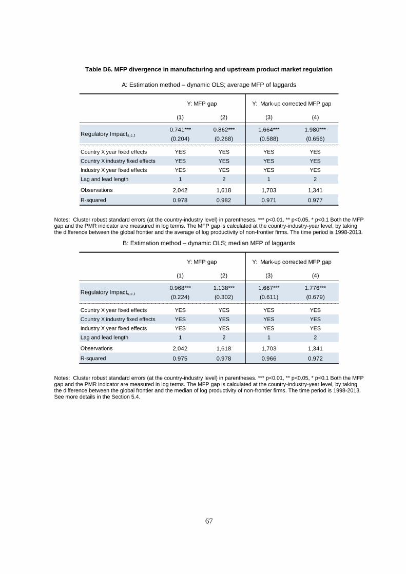
67
Table D6. MFP divergence in manufacturing and upstream product market regulation
A: Estimation method – dynamic OLS; average MFP of laggards
Notes: Cluster robust standard errors (at the country-industry level) in parentheses. *** p<0.01, ** p<0.05, * p<0.1 Both the MFP gap and the PMR indicator are measured in log terms. The MFP gap is calculated at the country-industry-year level, by taking the difference between the global frontier and the average of log productivity of non-frontier firms. The time period is 1998-2013.
B: Estimation method – dynamic OLS; median MFP of laggards
Notes: Cluster robust standard errors (at the country-industry level) in parentheses. *** p<0.01, ** p<0.05, * p<0.1 Both the MFP gap and the PMR indicator are measured in log terms. The MFP gap is calculated at the country-industry-year level, by taking the difference between the global frontier and the median of log productivity of non-frontier firms. The time period is 1998-2013. See more details in the Section 5.4.
(1) (2) (3) (4)
0.741*** 0.862*** 1.664*** 1.980***
(0.204) (0.268) (0.588) (0.656)
Country X year fixed effects YES YES YES YES
Country X industry fixed effects YES YES YES YES
Industry X year fixed effects YES YES YES YES
Lag and lead length 1 2 1 2
Observations 2,042 1,618 1,703 1,341
R-squared 0.978 0.982 0.971 0.977
Y: MFP gap Y: Mark-up corrected MFP gap
Regulatory Impacts,c,t
(1) (2) (3) (4)
0.968*** 1.138*** 1.667*** 1.776***
(0.224) (0.302) (0.611) (0.679)
Country X year fixed effects YES YES YES YES
Country X industry fixed effects YES YES YES YES
Industry X year fixed effects YES YES YES YES
Lag and lead length 1 2 1 2
Observations 2,042 1,618 1,703 1,341
R-squared 0.975 0.978 0.966 0.972
Y: MFP gap Y: Mark-up corrected MFP gap
Regulatory Impacts,c,t
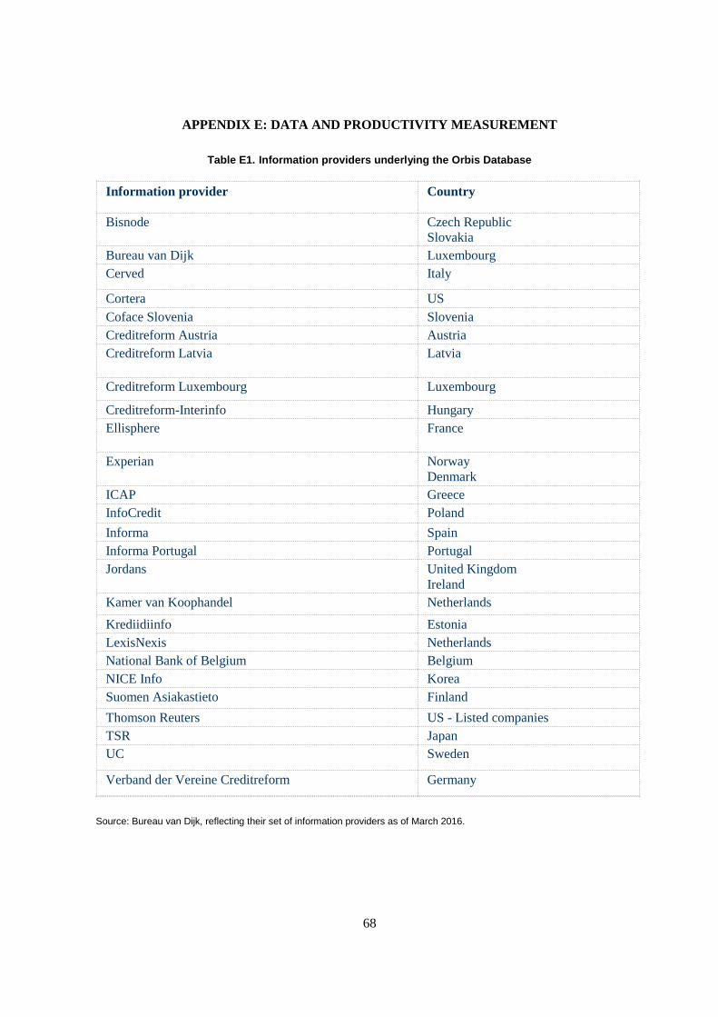
68
APPENDIX E: DATA AND PRODUCTIVITY MEASUREMENT
Table E1. Information providers underlying the Orbis Database
Information provider Country
Bisnode Czech Republic
Slovakia
Bureau van Dijk Luxembourg
Cerved Italy
Cortera US
Coface Slovenia Slovenia
Creditreform Austria Austria
Creditreform Latvia Latvia
Creditreform Luxembourg Luxembourg
Creditreform-Interinfo Hungary
Ellisphere France
Experian Norway
Denmark
ICAP Greece
InfoCredit Poland
Informa Spain
Informa Portugal Portugal
Jordans United Kingdom
Ireland
Kamer van Koophandel Netherlands
Krediidiinfo Estonia
LexisNexis Netherlands
National Bank of Belgium Belgium
NICE Info Korea
Suomen Asiakastieto Finland
Thomson Reuters US - Listed companies
TSR Japan
UC Sweden
Verband der Vereine Creditreform Germany
Source: Bureau van Dijk, reflecting their set of information providers as of March 2016.
69
Data
This paper uses a harmonized firm-level productivity database, based on underlying data from the
recently updated OECD-Orbis database (see Gal, 2013). The database contains several productivity
measures (variants of labour productivity and multi-factor productivity, MFP) and covers up to 24
OECD countries over the period 1997 to 2014 for the non-farm, non-financial business sector.58 These
countries are: Austria, Belgium, Czech Republic, Denmark, Estonia, Finland, France, Germany, Great
Britain, Greece, Hungary, Ireland, Italy, Japan, Korea, Netherlands, Norway, Poland, Portugal, Spain,
Sweden, Slovenia, the Slovak Republic and the United States. The country coverage is somewhat
smaller in the policy analysis, given the limited availability of the policy indicators, or lack thereof, for
some of the 24 countries considered. The industry coverage means retaining industries with 2 digit codes
from 5 to 82, excluding 64-66 in the European classification system NACE Rev 2, which is equivalent
to the international classification system ISIC Rev. 4 at the 2-digit level.
As discussed in Gal (2013), these data come from annual balance sheets and income statements,
collected by an electronic publishing firm called Bureau van Dijk, using a variety of underlying sources
ranging from credit rating agencies (e.g. Cerved in Italy) to national banks (e.g. National Bank of
Belgium for Belgium) as well as financial information providers (e.g. Thomson Reuters for the US). See
the full list of information providers to Bureau van Dijk regarding financial information for the set of
countries retained in the analysis in Table E1.
Orbis is the largest cross-country company-level database that is available and accessible for economic
and financial research. However, since the information is primarily collected for use in the private sector
typically with the aim of financial benchmarking, a number of steps need to be undertaken before the
data can be used for economic analysis. The steps we apply closely follow suggestions by Kalemli-
Ozcan, Sorensen, Villegas-Sanchez, Volosovych and Yesiltas (2015) and previous OECD experience
(Gal, 2013). Three broad steps are (i) ensuring comparability of monetary variables across countries and
over time (PPP conversion and deflation); (ii) deriving new variables that will be used in the analysis
(capital stock, productivity); and (iii) keeping company accounts with valid and relevant information for
our present purposes (filtering or cleaning). Finally, Orbis is a subsample of the universe of companies
for most countries, retaining the larger and hence probably more productive firms. To mitigate problems
arising from this, we exclude firms with less than 20 employees on average over their observed lifespan.
Variable definitions
Value added is defined as the sum of gross profits and the costs of employees. More
specifically, value added is the sum of the following accounting categories as available from
earnings statements: Profit (net income) for the period + Depreciation + Taxation + Interests
paid + Cost of employees.
Capital stock is derived from the book value of fixed assets using the perpetual inventory
method on gross investments - deflated by 2-digit country-specific investment deflators – and
the initially observed fixed assets. Firm-specific depreciation rates are derived using the book
value of depreciation and fixed assets. Before running the production function estimations, a
number of additional cleaning rules were applied. In particular, within each 2-digit industry,
those observations are excluded where log(value added/employment), log(capital/employment)
and log (materials/employment) are outside the top or bottom 0.5% of their distribution. The
resulting productivity measures as well as the mark-up and capital intensity measures discussed
58 This means retaining industries with 2 digit codes from 5 to 82, excluding 64-66 in the European classification
system NACE Rev 2, which is equivalent to the international classification system ISIC Rev. 4 at the 2-digit level.
70
below are then also filtered by following a similar procedure, but applied only for growth rates
and not (log) levels since it is crucial for our purposes that we retain in the analysis the most
productive firms. Specifically, within each country, the top and bottom 0.5% of the annual
growth rate distribution of productivity, capital intensity and mark-ups are left out, to avoid the
influence of extreme outliers in terms of productivity (mark-up, capital-intensity) growth.
MFP: We employ the one-step GMM estimation method proposed by Wooldridge (2009),
which mitigates the endogeneity problem of input choices by using material inputs as proxy
variables for productivity and (twice) lagged values of labour as instruments. This approach
builds on Levinsohn and Petrin (2003) but addresses the critique of Ackerberg et al (2015) on
the identification of the labour coefficient, and also makes estimations more efficient and robust
since it avoids using a two-step approach. To avoid limiting sample size unnecessarily, the MFP
measures are also calculated for those firms where intermediate inputs are not observed. With
the actual implementation of Wooldridge (2009) in software code (in Stata) we follow the
program codes provided by Petrin and Levinsohn (2012).
The production function is estimated separately for each 2-digit industry but pooled across all
countries, controlling for country and year fixed effects. This allows for inherent technological
differences across industries, while at the same time ensures comparability of MFP levels across
countries and over time by having a uniform labour and capital coefficient along these
dimensions.
The estimated coefficients are statistically significant and economically meaningful in that the
labour coefficients tend to be higher in services than in manufacturing and overall they range
between 0.6 and 0.85. The production function estimation results are available upon request. In
order to maximize coverage for our MFP measures, they are also calculated as a residual from
the estimated production function for those firms where materials (our measure of intermediate
inputs) are not available. However, the first step of the mark-up estimation also relies on
materials, hence the sample size reduction in the mark-up corrected MFP measures.
Deflation and currency conversion
Real values are obtained by applying 2-digit industry value added deflators from detailed OECD
National Accounts. This uses the ISIC Rev. 4 variant of the classification of activities. If deflators are
missing at the two-digit industry detail, they are filled up by applying the growth rate in the price index
at the immediate higher level of aggregation. For instance, if textile manufacturing (industry code 13)
has missing information on the value added deflator for a particular country in a particular year, the
growth rate from the immediate higher level (Textiles and wearing apparel, industry group 13-14) is
used. If that is missing as well, then once more the immediate higher level (Textiles, wearing apparel,
leather and related products industry group 13-15) is used. The same practice is followed for the other
deflators used in the paper: gross output, value added, intermediate inputs and gross fixed capital
formation.
We use the country-industry level purchasing power parity database of Inklaar and Timmer (2014), see
details therein for the trade-offs involved in deriving their PPP measures.
Filtering and cleaning
In order to limit the influence of erratic or implausible firm-behaviour, we exclude information for firms
that report an extreme annual log-change (growth). More precisely, the variable is set to missing for the
whole observed life of the firm if at least once, the variable has a growth rate that is in the top or bottom
1% of the growth distribution, at least once during their observed period. We do this procedure for the
71
following variables: labour productivity measures, MFP measures, employment, capital, capital ratio,
intermediates, value added and gross output. The rationale behind being relatively strict is that when a
big growth rate – i.e. level shift – is observed, it is difficult to know whether the pre- or the post- shift
period should be retained for the analysis. By removing the whole firm, we are also likely to exclude
cases when a firm purchased another (relatively large) one as well as when a firm is being split-up.
Representativeness issues
A key drawback of Orbis is that it is a selected sample of larger and more productive firms and thus
tends to under-represent smaller and younger firms in some economies. Accordingly, we exclude firms
with less than 20 employees. Even so, the analysis of the MFP growth of laggard firms should be
interpreted with particular caution, to the extent that laggards are likely to be less well represented in
the sample.
While this issue is probably less of a concern for firms at the national and global frontier, some other
issues remain. For example, the reporting unit (establishment or firm) may be different across countries.
A related issue is that countries may apply different accounting requirements. For instance, US
companies in Orbis report their financial statement in a consolidated manner, while in most European
countries the database contains mainly unconsolidated accounts.59 Accordingly, the coverage of Orbis
is less satisfactory for the United States than many European countries, although its coverage of US
affiliates abroad is still good. Furthermore, multinational firms may systematically shift profits across
the countries in which they have affiliates, depending on the tax system of the countries of its affiliates
(see OECD 2013). A priori, it is not clear in which direction these factors will bias the analysis given
that the focus is only on the global frontier and the gap relative to “all laggard firms” and thus country
boundaries are less relevant. However, it is reassuring that the key result of Section 4 – i.e. that global
frontier firms have become relatively more productive over the 2000s compared to other firms – is robust
to excluding firms that are part of a multi-national group (i.e. headquarters or subsidiaries) where profit-
shifting activity may be relevant. However, this comes at the cost of significantly reducing the number
of observations, so it is not incorporated in the baseline specification but is instead presented as a
robustness test (Appendix A).
Another caveat is that emerging market economies are not well represented in the database hence they
are not included in our analysis. While this is unlikely to significantly affect the measurement of the
global productivity frontier, it may have implications for diffusion if global frontier technologies are
increasingly diffusing to firms in emerging markets but not to those in OECD economies. However, this
seems unlikely, in light of the evidence presented in Comin and Mestieri (2013) which highlights
impediments related to the penetration of new technologies across a sample of developed and developing
economies alike.
The composition of countries in the frontier is probably still not entirely accurate, as the Orbis database
has a low coverage of US company accounts that are suitable for productivity analysis (Gal, 2013).
Nevertheless, as discussed in Andrews, Criscuolo and Gal (2015), firms located in the United States,
and other highly developed countries, are well-represented in the global frontier grouping. Moreover,
59 Working with a mix of the two types of accounts carries the risk of double counting certain activities if a firm files
both consolidated and unconsolidated accounts. However, the aim of this paper is not to measure aggregate
economic activity but to analyse the determinants of firms’ behaviour. Thus, the ideal reporting and consolidation
level (i.e. group, firm or establishment) should be the one that most closely reflects managerial decisions. It is a
difficult task to judge a priori which level that is, but most of the literature assumes it is either the firm or the group. For these reasons, we give priority to consolidated accounts by removing the unconsolidated ones for companies
where both types of accounts are present in the data.

72
this definition of the global frontier seems to match anecdotal evidence with for example Finland and
Korea having firms at the global frontier in most ICT sectors, or Italy being well represented at the
global frontier in the textiles industry.