Embed Size (px)
Citation preview
arX
iv:d
g-ga
/950
3016
v1 3
1 M
ar 1
995
dg-ga/9503016DAMTP 95-17
Symmetric Monopoles
N.J. Hitchin1, N.S. Manton2,
M.K. Murray3
Abstract We discuss SU(2) Bogomolny monopoles of arbitrary charge k invariantunder various symmetry groups. The analysis is largely in terms of the spectral curves,the rational maps, and the Nahm equations associated with monopoles. We considermonopoles invariant under inversion in a plane, monopoles with cyclic symmetry,and monopoles having the symmetry of a regular solid. We introduce the notion of astrongly centred monopole and show that the space of such monopoles is a geodesicsubmanifold of the monopole moduli space.
By solving Nahm’s equations we prove the existence of a tetrahedrally symmetricmonopole of charge 3 and an octahedrally symmetric monopole of charge 4, anddetermine their spectral curves. Using the geodesic approximation to analyse thescattering of monopoles with cyclic symmetry, we discover a novel type of non-planark-monopole scattering process.
AMS classification scheme numbers: 53C07, 81T13, 32L05
1. Department of Pure Mathematics and Mathematical Statistics, University of Cam-bridge, 16 Mill Lane, Cambridge CB2 1SB, U.K. [email protected]. Department of Applied Mathematics and Theoretical Physics, University of Cam-bridge, Silver Street, Cambridge CB3 9EW, U.K. [email protected]. Department of Pure Mathematics, The University of Adelaide, Adelaide SA 5005,Australia. [email protected]
1 Introduction
In recent years, there has been considerable interest in monopoles, which are particle-like solitons in a Yang-Mills-Higgs theory in three spatial dimensions. In this paper,we shall consider SU(2) Bogomolny monopoles, which are the finite energy solutionsof the Bogomolny equations (1), [5]. Solutions are labelled by their magnetic charge,a non-negative integer k, and are physically interpreted as static, non-linear superpo-sitions of k unit charge magnetic monopoles. There is a 4k-dimensional manifold ofsolutions up to gauge equivalence, known as the k-monopole moduli space Mk, andon this there is a naturally defined Riemannian metric, which is hyperkahler [1].
For monopoles moving at modest speeds compared with the speed of light, it isa good approximation to model k-monopole dynamics by the geodesic motion on themoduli space Mk. This was conjectured some time ago [20], and the consequencesexplored in some detail [1, 10, 28, 3, 26]. Very recently, the validity of the geodesicapproximation has been proved analytically by Stuart [24].
Most studies of Bogomolny monopoles have been concerned either with the generalstructure of the k-monopole moduli space Mk and its metric, or with a detailed studyof the geodesics on it for small values of k. Little work has been done on k-monopoledynamics for k > 2. In this paper, we investigate classes of k-monopole solutionswhich are invariant under various symmetry groups and derive results on their scat-tering. We consider monopoles invariant under inversion in a fixed plane, monopolesinvariant under a cyclic group of rotations about a fixed axis, and monopoles invariantunder the symmetry groups of the regular solids, that is, the tetrahedral, octahedraland icosahedral groups. The existence of k-monopoles with cyclic symmetry was pre-viously shown in [22]. Each submanifold of the moduli space Mk consisting of allk-monopoles invariant under a fixed symmetry group is a totally geodesic submani-fold. We therefore obtain various examples of monopole scattering with symmetry,by finding geodesics on such submanifolds.
Among our most interesting results are proofs of existence of a tetrahedrally sym-metric charge 3 monopole and an octahedrally symmetric charge 4 monopole. Wegive explicit formulae for the spectral curves and the solutions of Nahm’s equationscorresponding to these monopoles. Our approach rather strongly indicates that thereshould be an icosahedrally symmetric monopole of charge 6, but a detailed study ofNahm’s equations shows, surprisingly, that such an object does not exist.
Much of the motivation for the present study of symmetric monopoles came fromresults concerning Skyrmions. Skyrmions are SU(2)-valued scalar fields in R3 whichminimize Skyrme’s energy functional. They have an integer topological charge B,physically identified with baryon number. Numerical work by Braaten et al. [6] hasestablished that the Skyrmions of charges one to four have, respectively, sphericalsymmetry, toroidal symmetry, tetrahedral symmetry and octahedral symmetry. Sim-
1
ilar results have subsequently been obtained using instanton-generated Skyrmions[2, 18]. Since a unit charge monopole is spherically symmetric, and the maximalsymmetry of a charge 2 monopole is that of a torus, we were led to seek monopoles ofcharge 3 and charge 4 with tetrahedral and octahedral symmetry, respectively. TheSkyrmions of charge 5 and charge 6 are also known, and have rather low symmetry,so the absence of an icosahedrally symmetric charge 6 monopole is not so surprising.We should remark that the relationship between Skyrmions and monopoles is notsystematically understood. A B = 1 Skyrmion has six degrees of freedom, whereas aunit charge monopole has four. The moduli space of charge k monopoles has dimen-sion 4k. There is a less well-defined moduli space of Skyrme fields of baryon numberB, of dimension 6B, and a well-defined space of instanton-generated Skyrme fields ofdimension 8B − 1. It would be interesting if the charge B monopole moduli spacecould be identified as a submanifold of either of these latter spaces. This is certainlypossible for B = 2 [2].
In Section 2 we review monopoles and their moduli spaces. Further details ofthis material can be found in the book [1] and in the references contained therein. InSection 3 we review the spectral curves and rational maps associated with monopoles.In Section 4 we show how the rational map changes when a monopole is inverted inthe plane with respect to which the rational map is defined, and we investigate themonopoles which are invariant under this inversion. In Section 5 we consider theholomorphic geometry associated with the centre of a monopole. We define the totalphase of a monopole, and introduce the notion of a strongly centred monopole – onewhose centre is at the origin and whose total phase is 1. The manifold of stronglycentred monopoles is totally geodesic in Mk; in fact up to a k-fold covering, it splitsoff isometrically.
Spectral curves of k-monopoles are curves in TP1, the tangent bundle to thecomplex projective line, satisfying a number of constraints. In Section 6 we considerthe action of symmetry groups on general curves in TP1, and present various classesof curves with cyclic or dihedral symmetry, and with the symmetries of regular solids.These are candidates for the spectral curves of symmetric monopoles. In Section 7we show that the simplest curves with the symmetries of the regular solids are relatedto elliptic curves.
In Sections 8 to 11 we review the Nahm equations associated with monopoles andconsider the existence of symmetric monopoles and the corresponding solutions ofNahm’s equations. These equations are in general very difficult to solve explicitly,involving theta functions of curves of high genus [9]. Rather conveniently, the symme-try conditions imposed here reduce the solutions to ones written in terms of ellipticfunctions. We prove thereby the existence of a tetrahedrally symmetric monopole ofcharge 3 (Theorem 1), and an octahedrally symmetric monopole of charge 4 (Theo-rem 2), and we determine their spectral curves. We also prove the non-existence of
2
an icosahedrally symmetric monopole of charge 6 (Theorem 3).In Section 12, we investigate k-monopoles symmetric under the cyclic group Ck.
By considering the Ck-invariant rational maps, we show that the strongly centredmonopoles with Ck symmetry are parametrized by a number of geodesic surfacesof revolution in the moduli space Mk. Geodesic motions on these surfaces modeleither a purely planar k-monopole scattering process, or a novel type of k-monopolescattering, in which k unit charge monopoles collide simultaneously in a plane andan l-monopole and a (k − l)-monopole emerge back-to-back along the line throughthe k-monopole centre, perpendicular to the plane. The outgoing monopole clustersboth become axisymmetric about this line as their separation increases to infinity.When k = 3 and l = 1 or l = 2, this geodesic motion passes instantaneously throughthe tetrahedrally symmetric 3-monopole (oppositely oriented in the two cases), andwhen k = 4 and l = 2, through the octahedrally symmetric 4-monopole.
Finally a warning is necessary for the reader who wishes to delve into the literatureon this subject. There are a number of places in the theory of monopoles where onehas to make choices and establish conventions. Most of these are to do with theorientation of R3 and the induced complex structure on the twistor space TP1 of alloriented lines in R3. Different authors have made different conventions, and minorinconsistencies can appear to result if the literature is only read in a cursory manner.
2 Monopoles
To define a monopole we start with a pair (A, φ) consisting of a connection 1-formA on R3 with values in su(2), the Lie algebra of SU(2), and a function φ (the Higgsfield) from R3 into su(2). The Yang-Mills-Higgs energy on this pair is
E(A, φ) =∫
R3
(|FA|2 + |∇Aφ|2)d3x
where FA = dA + A ∧ A is the curvature of A, ∇Aφ = dφ + [A, φ] is the covariantderivative of the Higgs field, and we use the usual norms on 1-forms and 2-forms andthe standard inner product on su(2). The energy is minimized by the solutions of theBogomolny equations [5]
⋆ FA = ∇Aφ (1)
where ⋆ is the Hodge star on forms on R3. These equations, and the energy, areinvariant under gauge transformations, where the gauge group G of all maps g fromR3 to SU(2) acts by
(A, φ) 7→ (gAg−1 − dgg−1 , gφg−1).
3
Finiteness of the energy, and the Bogomolny equations, imply certain boundary con-ditions at infinity in R3 on the pair (A, φ) which are spelt out in detail in [1]. Inparticular, |φ| → c for some constant c which cannot change with time. Following[1], we fix c = 1.
A monopole, then, is a gauge equivalence class of solutions to the Bogomolnyequations subject to these boundary conditions. In some suitable gauge there is awell-defined Higgs field at infinity
φ∞:S2∞ → S2 ⊂ su(2)
going from the two sphere of all oriented lines through the origin in R3 to the unittwo-sphere in su(2). The degree of φ∞ is a positive integer k called the magneticcharge of the monopole.
Before discussing the moduli space of all solutions of the Bogomolny equationswe need to be a little more precise and talk about framed monopoles. We say a pair(A, φ) is framed if
limx3→∞
φ(0, 0, x3) =(i 00 −i
).
The gauge transformations fixing such pairs are those g with limx3→∞ g(0, 0, x3) diag-onal. Notice that every monopole can be gauge transformed until it is framed. So thespace of monopoles modulo gauge transformations is the same as the space of framedmonopoles modulo those gauge transformations that fix them. We define a framedgauge transformation to be one such that limx3→∞ g(0, 0, x3) = 1. The quotient of theset of all framed monopoles of charge k by the group of framed gauge transformationsis a manifold called the moduli space of (framed) monopoles of charge k and denotedMk. The group of constant diagonal gauge transformations (a copy of U(1)) acts onMk and the quotient is called the reduced moduli space Nk. This action is not quitefree, because the element −1 acts trivially, but the group U(1)/{±1} acts freely onMk.
The dimension of Mk is 4k, which can be understood as follows. In the casethat k = 1 there is a spherically symmetric monopole called the Bogomolny-Prasad-Sommerfield (BPS) monopole, or unit charge monopole. Its Higgs field has a singlezero at the origin, and its energy density is peaked there so it is reasonable to thinkof the origin as the centre or location of the monopole. The Bogomolny equations aretranslation invariant so this monopole can be translated about R3 and also rotatedby the circle of constant diagonal gauge transformations. This in fact generates allof M1 which is therefore diffeomorphic to S1 × R3. The coordinates on M1 specifythe location of the monopole and what can be thought of as an internal phase. Moregenerally there is an asymptotic region of the moduli space consisting of approximatesuperpositions of k unit charge monopoles located at k widely separated points andwith k arbitrary phases.
4
Although it is not possible to assign precisely to a charge k monopole k points orlocations in R3 it is possible to assign to the monopole a centre which can be thoughtof as the average of the locations of the k particles making up the monopole. Theimportant property of this centre is that if we act on the monopole by an isometryof R3 the centre moves by the same isometry. It is also possible to assign to a k-monopole a total phase; this is essentially the product of the phases of the k unitcharge monopoles. If we act on the monopole by a constant diagonal gauge trans-formation corresponding to an element µ of U(1) then the total phase changes byµ2k.
The natural metric on the moduli space Mk is obtained as follows. There is aflat L2 metric on the space of fields (A, φ), and this descends to a curved metric onthe space of gauge equivalence classes of fields. The latter metric, restricted to thek-monopole solutions of the Bogomolny equations is the metric on Mk. Since a largepart of the moduli space Mk describes k well-separated unit charge monopoles, manygeodesics on Mk correspond to the scattering of k unit charge monopoles, and weshall discuss below some particularly symmetric cases of such scattering.
3 Spectral curves and rational maps
It is not easy to study charge k monopoles directly in terms of their fields (A, φ).However, there are various ways of transforming monopoles to other types of math-ematical objects. There is a twistor theory for monopoles and the result of applyingthis shows that monopoles are equivalent to a certain class of holomorphic bundles onthe so-called mini-twistor space TP1. The boundary conditions of the monopole implythat the holomorphic bundle is determined by an algebraic curve, called the spectralcurve. Monopoles that differ only by a constant diagonal gauge transformation havethe same spectral curve, see [11, 12].
The holomorphic bundle of a k-monopole is defined as follows [11]. Let γ be anoriented line in R3 and let ∇γ denote covariant differentiation using the connectionA along γ. One considers the ordinary differential equation
(∇γ − iφ)v = 0 (2)
where v : γ → C2. The vector space Eγ of all solutions to equation (2) is two-dimensional and the union of all these spaces forms a rank two smooth complexvector bundle E over the space of all oriented lines in R3. It can be shown that thisspace of all oriented lines is a complex manifold, in fact isomorphic to TP1. Onemay define on E a holomorphic structure if the monopole satisfies the Bogomolnyequations. The bundle E has two holomorphic sub-bundles E±
1 whose fibres (E±1 )γ
at γ are defined to be the spaces of solutions that decay as ±∞ is approached along
5
the line γ. The set of γ where (E+1 )γ = (E−
1 )γ , so there is a solution decaying at bothends, forms a curve S in TP1 called the spectral curve of the monopole. It is possibleto show that a decaying solution decays exponentially so the spectral curve is alsothe set of all lines along which there is an L2 solution. Intuitively one should thinkof the spectral lines as being the lines going through the locations of the monopoles.In the case of charge 1, the spectral lines are precisely those going through the centreof the monopole.
If we describe a typical point in P1 by homogeneous coordinates [ζ0, ζ1] then wecan cover P1, in the usual way, by two open sets U0 and U1 where ζ0 and ζ1 arenon-zero, respectively. On the set U0 we introduce the coordinate ζ = ζ1/ζ0. Let usalso denote by U0 and U1 the pre-images of these sets under the projection map fromTP1 to P1. Then a tangent vector η∂/∂ζ at ζ in U0 can be given coordinates (η, ζ).These coordinates allow us to describe an important holomorphic line bundle L onTP1 which has transition function exp(η/ζ) on the overlap of U0 and U1. Similarly forany complex number λ we define the bundle Lλ by the transition function exp(λη/ζ).Finally, if n is any integer we define the line bundle Lλ(n) to be the tensor productof Lλ with the n-th power of the pull-back under projection TP1 → P1 of the dual ofthe tautological bundle on P1. This has transition function ζ−n exp(λη/ζ). The linebundle L0 is clearly trivial so we denote it by O, and L0(n) is denoted by O(n).
Another way of introducing the twistor theory for monopoles is to note, as in[19], that the Bogomolny equations on R3 are equivalent to the self-dual Yang-Millsequations on R4, invariant under translation in the fourth direction, so monopoles areequivalent to S1-invariant instantons on S1 ×R3. The twistor space Z for S1×R3 isthe quotient of P3\P1 by a free Z-action, and is a bundle of groups C∗ ×C over P1.By the original Atiyah-Ward construction, an instanton corresponds to a holomorphicbundle on the twistor space Z, and if it is S1-invariant, it descends to Z/C∗ = TP1.The space Z itself is the total space of the principal bundle for the line bundle Ldefined above by transition functions.
To avoid the potential ambiguity in what we mean by ‘transition function’ let usbe more explicit. The line bundle Lλ(n) has non-vanishing holomorphic sections χ0
and χ1 over U0 and U1 respectively and for points in U0 ∩ U1 these satisfy
χ0 = ζ−n exp(λη
ζ)χ1. (3)
If we consider an arbitrary holomorphic section f of this line bundle its restrictionto U0 and U1 can be written as f = f0χ0 and f = f1χ1 respectively where f0 andf1 are holomorphic functions on U0 and U1. As a consequence of equation (3) thesefunctions must satisfy
f0 = ζn exp(−λη
ζ)f1 (4)
6
at points in the intersection U0 ∩ U1.With these definitions we can present the results that we need. The sub-bundles
E±1 satisfy E±
1 ≃ L±1(−k) and the quotients satisfy E/E±1 ≃ L∓1(k). For a framed
monopole there are explicit isomorphisms so we shall write = instead of ≃. Thecurve S is defined by the vanishing of the map E+
1 → E/E−1 and hence by a section
of (E+1 )
∗ ⊗ E/E−1 = O(2k). In terms of the coordinates (η, ζ), S is defined by an
equation of the form
P (η, ζ) ≡ ηk + ηk−1a1(ζ) + . . .+ ηak−1(ζ) + ak(ζ) = 0, (5)
where, for 1 ≤ r ≤ k, ar(ζ) is a polynomial in ζ of degree at most 2r.The space TP1 has a real structure τ , namely, the anti-holomorphic involution
defined by reversing the orientation of the lines in R3. In coordinates it takes theform τ(η, ζ) = (−η/ζ2,−1/ζ). The curve S is fixed by this involution, so we say thatit is real. The reality of S implies that for 1 ≤ r ≤ k,
ar(ζ) = (−1)rζ2rar(−1
ζ). (6)
If k = 1 the spectral curve has the form
η = (x1 + ix2)− 2x3ζ − (x1 − ix2)ζ2
where x = (x1, x2, x3) is any point in R3, [[11], eq. (3.2)]. Such a curve is called areal section as it defines a section of the bundle TP1 → P1, and is real in the sensegiven above. In terms of the geometry of R3 this curve is the set of all oriented linesthrough the point x, so it is the spectral curve of a BPS monopole located at x. Werefer to this curve as the “star” at x.
In [11, 12] one can find listed all the properties that a curve in TP1 has to satisfyto be a spectral curve. We are interested in one of these here. From the definitionof the spectral curve we see that over the spectral curve the line bundles E+
1 andE−
1 coincide as sub-bundles of E; in particular they must be isomorphic. This isequivalent to saying that the line bundle E+
1 ⊗ (E−1 )
∗ = L2 is trivial over the curveor that it admits a non-vanishing holomorphic section s. The real structure τ can belifted to an anti-holomorphic, conjugate linear map between the line bundles L2 andL−2 and hence the section s can be conjugated to define a new (holomorphic) sectionτ(s) = τ ◦s◦τ of L−2 over S. Tensoring these defines a section τ(s)s of L−2⊗L2 = Oand because S is compact and connected this is a constant. Because of the framingthis constant will be 1. Notice that given only S and the fact that L2 is trivial over S,if we can choose a section s such that τ(s)s = 1 then it is unique up to multiplicationby a scalar of modulus one. This circle ambiguity in the choice of s corresponds to
7

the framing of the monopole. In fact, let µ be a complex number of modulus onecorresponding to a constant diagonal gauge transformation with diagonal entries µand µ−1. Then it is possible to follow through the proof in ([11], pp. 593-4) and showthat if we phase rotate a framed monopole by µ, the isomorphism E+
1 → L(−k) ismultiplied by µ and the isomorphism E−
1 → L∗(−k) is multiplied by µ−1. The sections of E+
1 ⊗ (E−1 )
∗ = L2 is therefore multiplied by µ2. Notice that this is consistentwith the fact that the group U(1)/{±1} acts freely on the moduli space Mk of framedmonopoles.
The rational map of a monopole was originally described by Donaldson in terms ofsolutions to Nahm’s equations [7]. Hurtubise then showed how it relates to scatteringin R3 and to the spectral curve of the monopole [14]. It will be convenient for ourpurposes to use the description in terms of spectral curves.
The rational map of a charge k monopole is from C to C⋃∞, and is simply
a polynomial p of degree less than k divided by a monic (leading coefficient = 1)polynomial q of degree k which has no factor in common with p,
R(z) =p(z)
q(z).
We shall denote by Rk the space of all these based rational maps. Donaldson hasproved that any such rational map arises from some unique charge k monopole [7],so Rk is diffeomorphic to Mk. The disadvantage of characterising a monopole byits rational map is that the definition of the map requires choosing a line and anorthogonal plane in R3, and this breaks the symmetries of the problem. Whereas theBogomolny equations are invariant under all the isometries of R3, the transformationto a rational map commutes only with those isometries that preserve the direction ofthe line.
To define the rational map we fix the fibre F of TP1 → P1 where ζ = 0 andidentify it with C. The fibre consists of all lines in the x3-direction. This correspondsto picking an orthogonal splitting of R3 as C×R. Each point z in C is identified witha point in F by setting z = η, and hence with an oriented line, the line {(x1, x2, x3) |x3 ∈ R} with z = x1 + ix2. The intersection of F with S defines k points countedwith multiplicity and q(z) is defined to be the unique monic polynomial of degreek which has these k points as its roots. Thus q(z) = P (z, 0), where P is given byeq. (5). Recall from (4) that a holomorphic section s of the bundle L2 is determinedlocally by functions s0 and s1, on U0 ∩ S and U1 ∩ S respectively, such that
s0(η, ζ) = exp(−2η
ζ)s1(η, ζ). (7)
Let p(z) be the unique polynomial of degree k−1 such that p(z) = s0(z, 0) mod q(z).The rational map of the monopole is then R(z) = p(z)/q(z). If the roots of q(z) are
8
distinct complex numbers β1, . . . , βk then the polynomial p(z) is determined by itsvalues p(βi) = s0(βi, 0) for all i = 1, . . . , k.
Let us make a brief remark about the construction of the rational map as scatteringdata in R3. More details are given in [14] and [1]. The points where S intersects F ,the zeros of q, correspond to the lines in the x3-direction admitting a solution ofeq.(2) decaying at both ends. Assume these lines are distinct and label them by thecorresponding complex numbers βi. Pick for each line a solution v(βi, x3) decayingat both ends. In the regions where x3 is large positive and large negative there arechoices of asymptotically flat gauge such that
limx3→∞
(x3)−k/2ex3v(βi, x3) = v+i
(10
)
and
limx3→−∞
(x3)−k/2e−x3v(βi, x3) = v−i
(01
).
The rational map with our conventions is determined by
p(βi) =v+iv−i
.
This agrees with the results stated in Chapter 16 of ref.[1], although Hurtubise’sconventions give p(βi) = v−i /v
+i .
We deduce from these formulae the action of certain isometries on the rationalmaps of monopoles. Let λ ∈ U(1) and w ∈ C define a rotation and translation,respectively, in the plane C. Let t ∈ R define a translation perpendicular to theplane and let µ ∈ U(1) define a constant diagonal gauge transformation. A rationalmap R(z) then transforms under the composition of all these transformations to
R(z) = µ2 exp(2t)λ−2kR(λ−1(z − w)).
Note that this is slightly different to the action described in [[1], eq. (2.11)], becauseof different conventions.
4 Inverting monopoles
Consider the inversion map I:R3 → R3 defined by I(x1, x2, x3) = (x1, x2,−x3). Thisinverts R3 in the (x1, x2) plane. The inversion map reverses orientation, and soinduces an anti-holomorphic map on the twistor space TP1 which we shall denote bythe same symbol and which in the standard coordinates on TP1 is
I(η, ζ) = (−η
ζ2,1
ζ).
9
To see this note that the real section defined by the point I(x1, x2, x3) has equation
η = (x1 + ix2) + 2x3ζ − (x1 − ix2)ζ2.
So a point I(η, ζ) is on this curve if and only if
−η
ζ2= (x1 + ix2) + 2x3
1
ζ− (x1 − ix2)
1
ζ2.
Conjugating this equation and clearing the denominators we recover
η = (x1 + ix2)− 2x3ζ − (x1 − ix2)ζ2,
the equation of the real section defined by the point (x1, x2, x3). This confirms theformula for I. Notice that I is very similar to the real structure τ ; in fact I ◦τ(η, ζ) =(η,−ζ).
If we invert the monopole defined by the spectral curve S and section s we obtaina new curve I(S) and a new section I(s). The definition of I(S) is straightforward; itis just the image of S under the map I. We shall consider I(s) in a moment. Becauseτ(S) = S it follows that (η, ζ) ∈ I(S) precisely when (η,−ζ) ∈ S. In particular, theintersection of I(S) and the fibre F over ζ = 0 is just the intersection of S and F .So if we denote by I(p) and I(q) the numerator and denominator of the rational mapfor the inverted monopole, we see that I(q) = q.
Now consider the section s. Notice that both τ and I interchange the two coordi-nate patches U0 and U1. The section τ(s) is defined locally by
τ(s)0(η, ζ) = s1(τ(η, ζ)) , τ(s)1(η, ζ) = s0(τ(η, ζ)) (8)
and the section I(s) by
I(s)0(η, ζ) = s1(I(η, ζ)) , I(s)1(η, ζ) = s0(I(η, ζ)). (9)
Hence I(p) is defined by
I(p)(z) = I(s)0(z, 0) mod q(z) = s1 ◦ τ(z, 0) mod q(z)
using the fact that τ(η, 0) = I(η, 0). From the relation τ(s)s = 1 and (8) it followsthat (s1 ◦ τ)s0 = 1 and hence
(I(p)p)(z) = (s1 ◦ τ(z, 0))s0(z, 0) mod q(z) = 1 mod q(z). (10)
Eq. (10), and the requirement that the degree of I(p) is less than k, determine I(p)uniquely. If the roots of q are the distinct complex numbers β1, . . . , βk, a usefulalternative way of obtaining I(p) is to notice that it is the unique polynomial ofdegree less than k such that I(p)(βi)p(βi) = 1 for all i = 1, . . . , k.
We summarize these results as:
10
Proposition 1 Let a monopole have spectral curve P (η, ζ) = 0 and rational mapp/q. The inverted monopole has spectral curve P (η,−ζ) = 0 and rational map I(p)/q,where I(p)p = 1 mod q.
It is interesting to consider the subset of monopoles that are invariant underinversion. Their spectral curves are given by polynomials P (η, ζ) which are even inζ . Their rational maps satisfy p2 = 1 mod q, so that I(p) = p. This fixed-point set isdescribed by the following:
Proposition 2 The moduli space IMk of k-monopoles invariant under inversion isa totally geodesic submanifold of Mk of dimension 2k. It has (k + 1) connected com-ponents IMm
k for 0 ≤ m ≤ k. The component IMmk is diffeomorphic to the set of
coprime pairs (r, s) of monic polynomials of degree m and (k −m) respectively.
Proof: It is a standard fact from differential geometry that the fixed point set of afinite group of isometries of a Riemannian manifold is a totally geodesic submanifold.For any rational function R = p/q defining a k-monopole, consider
f(R) =∑
i
p(βi)
This is a symmetric polynomial in the roots of q and hence is polynomial in thecoefficients of p and q, and so is continuous on Mk. On IMk, p
2 = 1 mod q, hencep(βi) = ±1. Thus, restricted to IMk, f takes the values k, k − 2, . . . ,−k, and wedefine IMm
k = f−1(k − 2m).If p2 − 1 = 0 mod q then q divides (p− 1)(p+1). Since these factors are coprime,
any irreducible factor of q divides one or the other. Hence we have monic polynomialsr, s of degrees m, k −m respectively, such that q = rs, and p+ 1 = 2ar, p− 1 = 2bsfor polynomials a, b. Hence p = ar + bs and ar − bs = 1.
Conversely, given two coprime monic polynomials r, s, the division algorithm im-plies that there exist polynomials a, b such that ar − bs = 1, and moreover a can bechosen uniquely to have degree less than that of s. Now define p = ar+ bs. This hasdegree less than k and
p2 = (ar + bs)2 = 1 + 4abq (11)
where q = rs is monic of degree k. Clearly, from (11), p and q are coprime and sodefine a rational map R.
Now the space of pairs (r, s) of coprime polynomials is the complement of a hy-persurface in Cm ×Ck−m and so is a connected 2k-dimensional manifold. Moreover,when r, s both have distinct roots, the roots of q are β1, . . . , βm and βm+1, . . . , βk (theroots of r and s respectively). Hence on this manifold f(R) = k − 2m, and so IMm
k
is connected, and as described in the proposition.
11
Note that IMmk and IMk−m
k are isomorphic; one is obtained from the other bymultiplying p by −1. The simplest of the components is IM0
k . Here p(z) ≡ 1, so therational maps are of the form
R(z) =1
q(z).
The space IM0k is naturally diffeomorphic to the moduli space of k flux vortices in the
critically coupled abelian Higgs model, since k-vortex solutions are also parametrisedby a single monic polynomial of degree k [25]. However, the metrics in the monopoleand vortex cases will be different.
We are not sure what kind of monopole configurations lie in the various spacesIMm
k , but we conjecture that for m = 0 (or m = k), the energy density is alwaysconfined to a finite neighbourhood of the plane x3 = 0, whereas for 0 < m < kit is possible for there to be monopole clusters arbitrarily far from the plane x3 =0, arranged symmetrically with respect to inversion in this plane. The examplesdiscussed in Section 12 are consistent with this conjecture. If the roots of q aredistinct and well-separated, then the configurations always consist of a set of unitcharge monopoles with their centres in the x3 = 0 plane.
Our inversion formula is inconsistent with Proposition 3.12 of [1]. There it wassuggested that if
R(z) =p(z)
q(z)=∑
i
αi
z − βi
is the rational map of a charge k monopole, which consists of k well-separated unitcharge monopoles, then (using our conventions) the individual monopoles are ap-proximately located at the points (βi, (1/2) log |αi|) and have phases αi|αi|−1. Con-sideration of our inversion formula suggests however that the individual monopolesare located at the points (βi, (1/2) log |p(βi)|) and have phases p(βi)|p(βi)|−1. Thishas recently been proved by Bielawski in [4]. Interestingly the spaces IMm
k play adistinguished role in Bielawski’s work.
Finally notice that it follows from equations (8) and (9) and the fact that τ(η, 0) =I(η, 0) that using τ(s) to construct the rational map is the same as using I(s), andhence the p(βi) occuring in the rational map defined using τ(s) would be the reciprocalof the p(βi) we use, and would give the rational map as defined by Hurtubise.
5 Centred monopoles and rational maps
We remarked earlier that although the positions and internal phases of the k ‘particles’in a charge k monopole are only asymptotically well-defined, every monopole has awell-defined centre and total phase. This arises naturally in the twistor picture. IfS is the spectral curve of a monopole then it intersects every fibre of TP1 → P1 in
12
k points counted with multiplicity. If we add these points together we obtain a newcurve which is given by an equation η + a1(ζ) = 0. This curve is a real section andhence a1 is of the form
a1(ζ) = −k((c1 + ic2)− 2c3ζ − (c1 − ic2)ζ2).
The point c = (c1, c2, c3) is the centre of the monopole. To define the total phaserequires a little more work.
Recall that the twistor space Z for S1 × R3 is the principal bundle for the linebundle L over TP1. Its quotient Z by ±1 ∈ C∗ is the principal bundle for L2. Thespectral curve S ⊂ TP1 has a trivialization s of L2 and hence lifts to Z. Thus, overeach point in P1, the spectral curve defines k points counted with multiplicity in thefibre. This fibre is the group C∗ ×C and we take the product of the points. This isa section sk of L2 over the curve η + a1(ζ) = 0.
The bundle L2 over any real section is trivial and we fix as a choice of trivialisationf over η − k((c1 + ic2)− 2c3ζ − (c1 − ic2)ζ
2) = 0
f0(η, ζ) = exp 2k(c3 + (c1 − ic2)ζ)f1(η, ζ) = exp 2k(−c3 + (c1 + ic2)/ζ).
It is easy to check that this non-vanishing section f satisfies τ(f)f = 1. Moreoverbecause τ(s)s = 1 we must have τ(sk)sk = 1. If we divide sk by f we obtain aholomorphic function which must be constant. In fact because τ(sk)sk = 1 andτ(f)f = 1 this constant is a complex number of modulus 1. We define sk/f to be thetotal phase of the monopole. Notice that if we act on the monopole by a constantdiagonal gauge transformation µ then s is replaced by µ2s and the total phase ismultiplied by µ2k.
Let us now see how to construct the centre and total phase of a monopole fromits rational map. Notice first that if we restrict the equation of the spectral curve tothe fibre ζ = 0 we obtain an equation of the form
ηk − k(c1 + ic2)ηk−1 + ... = 0
and hence c1 + ic2 is the average of the points of intersection of the spectral curvewith ζ = 0 or the average of the zeros of q.
Comparing the construction of the rational map of a monopole we see that
sk0(k(c1 + ic2), 0) =∏
i
p(βi) = △(p, q)
the resultant of p and q. It follows that
sk
f= △(p, q) exp(−2kc3).
So:
13
Proposition 3 If R(z) = p(z)/q(z) is the rational map of a monopole with q0 theaverage of the roots of q and △(p, q) the resultant of p and q, then the centre of themonopole is
(q0, (1/2k) log |△(p, q)|)and the total phase is
△(p, q)|△(p, q)|−1.
It follows that a monopole is centred if and only if the zeroes of q sum to zero and|△(p, q)| = 1. It will be useful to use a stronger notion of centring than this. Wecall a monopole strongly centred if it is centred and the total phase is 1. From whatwe have just proven a monopole is strongly centred if and only if its rational mapsatisfies
q0 = 0 and △(p, q) = 1. (12)
The resultant condition △(p, q) = 1 was used in [[1], p.30] to identify the universalcovering of the moduli space of centred monopoles, but for a fixed complex structurein the hyperkahler family. Our description of strong centring gives an invariant ap-proach, valid for all complex structures. Considered in the context of the twistorspace of a hyperkahler metric, it identifies the factor X in the isometric splitting [[1],p.34] Mk = X × S1 ×R3 of a k-fold covering of Mk with the space of strongly cen-tred monopoles. It follows that the space of strongly centred monopoles is a geodesicsubmanifold of Mk.
Remark: Note that the twistor space Z is the twistor space for the (trivial) hy-perkahler metric on the moduli space of 1-monopoles. A k-monopole’s centre andtotal phase then associates a 1-monopole with a Zk-ambiguity of phases to a k-monopole.
6 Symmetric curves in TP1
In eq. (5) we presented the general form of curves in TP1 that occur as spectral curvesof charge k monopoles. The coefficients ar(ζ) must satisfy the reality condition (6),and the curve is centred at the origin in R3 if a1(ζ) = 0. Here we shall discuss theform of these curves when they are required to be invariant under certain groups ofrotations about the origin.
Let us recall that in TP1, the P1 of lines through the origin are parametrized byζ with η = 0. The line in the direction of the Cartesian unit vector (x1, x2, x3) hasζ = (x1+ ix2)/(1+x3). It will be important to consider the homogeneous coordinates[ζ0, ζ1] on P1, as well as the inhomogeneous coordinate ζ = ζ1/ζ0. An SU(2) Mobius
14
transformation on the homogeneous coordinates, [ζ0, ζ1] → [ζ ′0, ζ′1], of the form
ζ ′0 = −(b+ ia)ζ1 + (d− ic)ζ0ζ ′1 = (d+ ic)ζ1 + (b− ia)ζ0
(13)
where a2 + b2 + c2 + d2 = 1, corresponds to an SO(3) rotation in R3. The rotationis by an angle θ about the unit vector (x1, x2, x3), where x1 sin
θ2= a, x2 sin
θ2=
b, x3 sinθ2= c, cos θ
2= d. The inhomogeneous coordinate ζ transforms to
ζ ′ =(d+ ic)ζ + (b− ia)
−(b+ ia)ζ + (d− ic). (14)
Since η is the coordinate in the tangent space to P1 at ζ , it follows that if ζ transformsto ζ ′ as in (14) then η transforms to η′ via the derivative of (14), that is
η′ =η
(−(b+ ia)ζ + (d− ic))2. (15)
A curve P (η, ζ) = 0 in TP1 is invariant under the Mobius transformation if P (η′, ζ ′) =0 is the same curve. If the curve is the spectral curve of a monopole, then the monopoleis invariant under the associated rotation.
The simplest group of symmetries is the cyclic group of rotations about the x3-axis, Cn. The generator is the Mobius transformation
ζ ′ = e2πi/nζ, η′ = e2πi/nη.
A curve P (η, ζ) = 0 is invariant if all terms of P have the same degree, mod n. Acurve of the form (5) is Cn-invariant if all terms have degree k, mod n. In particular,it is Ck-invariant if all terms have degree zero, mod k.
For there to be axial symmetry about the x3-axis, with symmetry group C∞, thecurve must be invariant under ζ → eiθζ, η → eiθη, for all θ. This requires that allterms in P (η, ζ) have degree k. There is a unique axially symmetric, strongly centredmonopole for each charge k. It is shown in [11] that its spectral curve is
η∏m
l=1(η2 + l2π2ζ2) = 0 for k = 2m+ 1
∏ml=0
(η2 + (l + 1
2)2π2ζ2
)= 0 for k = 2m+ 2.
Notice that these curves are not determined by symmetry alone, and that the coef-ficients of P are transcendental numbers. The only curve of the form (5) which hasfull SO(3) symmetry is ηk = 0. This is the spectral curve of a unit charge monopoleat the origin when k = 1, but for k > 1 it is not the spectral curve of a monopole.
15
The groups Cn and C∞ are extended to the dihedral groups Dn and D∞ by addinga rotation by π about the x1-axis. This rotation corresponds to the transformationon TP1
ζ ′ =1
ζ, η′ = − η
ζ2.
Under this transformation, and for any constant ν,
(η2 + νζ2)′ =1
ζ4(η2 + νζ2),
so each of the axially symmetric monopoles has symmetry group D∞.Recall from Section 4 that P (η, ζ) = 0 is reflection symmetric under x3 → −x3 if
P is even in ζ . By a similar argument to that in Section 4, the reflection x2 → −x2
corresponds to ζ → ζ, η → η, so a curve P (η, ζ) = 0 is invariant under this reflectionif all coefficients in P (η, ζ) are real. The axially symmetric monopoles therefore havethese reflection symmetries too.
As an example of finite cyclic or dihedral symmetry, let us consider centred k = 3curves with either C3 or D3 symmetry. Before imposing the symmetry, the curves areof the form
η3 + η(α4ζ4 + α3ζ
3 + α2ζ2 + α1ζ + α0)
+ (β6ζ6 + β5ζ
5 + β4ζ4 + β3ζ
3 + β2ζ2 + β1ζ + β0) = 0 (16)
subject to the reality conditions
α4 = α0, α3 = −α1, α2 = α2,β6 = −β0, β5 = β1, β4 = −β2, β3 = β3.
C3 symmetry implies that (16) reduces to
η3 + αηζ2 + βζ6 + γζ3 − β = 0 (17)
where α and γ are real. By a rotation about the x3-axis, we can orient the curve sothat β is real, too, and then there is reflection symmetry under x2 → −x2. There isD3 symmetry if γ = 0; then the curve reduces to
η3 + αηζ2 + β(ζ6 − 1) = 0 (18)
with α and β real.The axisymmetric charge 3 monopole has a spectral curve of type (18) with α = π2
and β = 0. Also, three well-separated unit charge monopoles at the vertices of an
16
equilateral triangle can have D3 symmetry. The spectral curve is asymptotic to theproduct of three stars at
(x1, x2, x3) ={(a, 0, 0), (a cos
2π
3, a sin
2π
3, 0), (a cos
4π
3, a sin
4π
3, 0)},
that is,(η − a(1− ζ2))(η − aω(1− ωζ2))(η − aω2(1− ω2ζ2)) = 0,
where ω = e2πi/3. Multiplied out, this is a curve of the form (18) with α = 3a2 andβ = a3, or equivalently α3 = 27β2. We shall find out more about the spectral curvesof charge 3 monopoles with symmetry C3 or D3 when we consider the rational mapsassociated with the monopoles (see Section 12).
Symmetry under C4 is rather a weak constraint on curves with k = 4. On theother hand D4 symmetry implies that a k = 4 curve is of the form
η4 + αη2ζ2 + βζ8 + γζ4 + β = 0 (19)
with α, β and γ real. The axisymmetric charge 4 monopole has this form of spectralcurve, with α = (5/2)π2, β = 0 and γ = (9/16)π4. Four well-separated unit chargemonopoles at the vertices of the square {(±a, 0, 0), (0,±a, 0)} can have D4 symmetry.The spectral curve is asymptotic to a product of stars, and is of the form (19),with α = 4a2, β = −a4 and γ = 2a4. After a π/4 rotation, the monopoles are at(±a/
√2,±a/
√2, 0), and α = 4a2, β = a4 and γ = 2a4.
There is another interesting asymptotic 4-monopole configuration, with a spectralcurve of type (19). Consider two well-separated axisymmetric charge 2 monopoles,centred at (0, 0, b) and (0, 0,−b), and with the x3-axis the axis of symmetry. Thespectral curve is asymptotic to a product of curves associated with the charge 2monopoles. The spectral curve of a centred axisymmetric charge 2 monopole is η2 +14π2ζ2 = 0. This factorizes as (η + 1
2iπζ)(η − 1
2iπζ) = 0, which is a product of stars
at the complex conjugate points (0, 0,±iπ/4). Translation by b gives the curve
η2 + 4bηζ + (4b2 +1
4π2)ζ2 = 0
which is the product of stars at (0, 0, b± iπ/4). Similarly, translation by −b gives
η2 − 4bηζ + (4b2 +1
4π2)ζ2 = 0
and the product of these is the curve
η4 + (1
2π2 − 8b2)η2ζ2 + (4b2 +
1
4π2)2ζ4 = 0.
17
Since all terms have degree 4 this curve is axisymmetric; however, the actual spectralcurve of the charge 4 monopole has symmetry D4, as we shall see in Section 12,becoming axisymmetric only in the limit of infinite separation.
Let us now investigate the curves in TP1 with the symmetries of a regular solid.Some of these are special cases of the curves we have already discussed. There arethree rotational symmetry groups to consider, those of a tetrahedron, an octahedronand an icosahedron. The direct way to construct a symmetric curve is to find Mobiustransformations which generate the symmetry group, and calculate the conditions forthe curve to be invariant under all of them. For example, a curve of type (19), withD4 symmetry, has octahedral symmetry if it is invariant under the transformation
ζ ′ =iζ + 1
ζ + i, η′ =
−2
(ζ + i)2η,
which corresponds to a π/2 rotation about the x1-axis, and this requires that thecurve reduces to
η4 + β(ζ8 + 14ζ4 + 1) = 0.
A more powerful and less laborious approach is to use the theory of invariant bilinearforms and polynomials on P1, as expounded in Klein’s famous book [15].
Consider a homogeneous bilinear form Qr(ζ0, ζ1) of degree r, and its associatedinhomogeneous polynomial qr(ζ) defined by
Qr(ζ0, ζ1) = ζr0qr(ζ).
Generally qr has degree r, but it may have lower degree. SupposeQr(ζ0, ζ1) is invariantunder a Mobius transformation of the form (13). Then qr(ζ) transforms in a simpleway under the corresponding transformation (14), namely
q′r(ζ) =qr(ζ)
(−(b+ ia)ζ + (d− ic))r. (20)
On the other hand, η transforms as in (15). Consider a centred curve in TP1,
P (η, ζ) ≡ ηk + ηk−2q4(ζ) + ηk−3q6(ζ) + . . .+ q2k(ζ) = 0.
If, under a Mobius transformation, each polynomial qr(ζ) transforms as in (20), andη as in (15), then each term in the polynomial P (η, ζ) is multiplied by the same factor(−(b+ ia)ζ + (d− ic))−2k, so the curve is invariant. It follows that curves invariantunder the rotational symmetry group of a regular solid can be constructed from theinhomogeneous polynomials qr derived from the bilinear forms Qr invariant under thegroup.
18
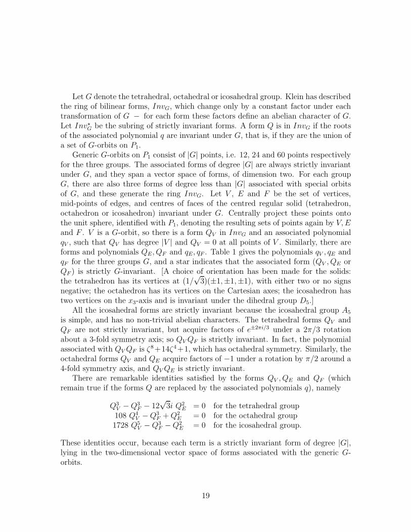
Let G denote the tetrahedral, octahedral or icosahedral group. Klein has describedthe ring of bilinear forms, InvG, which change only by a constant factor under eachtransformation of G − for each form these factors define an abelian character of G.Let Inv⋆G be the subring of strictly invariant forms. A form Q is in InvG if the rootsof the associated polynomial q are invariant under G, that is, if they are the union ofa set of G-orbits on P1.
Generic G-orbits on P1 consist of |G| points, i.e. 12, 24 and 60 points respectivelyfor the three groups. The associated forms of degree |G| are always strictly invariantunder G, and they span a vector space of forms, of dimension two. For each groupG, there are also three forms of degree less than |G| associated with special orbitsof G, and these generate the ring InvG. Let V , E and F be the set of vertices,mid-points of edges, and centres of faces of the centred regular solid (tetrahedron,octahedron or icosahedron) invariant under G. Centrally project these points ontothe unit sphere, identified with P1, denoting the resulting sets of points again by V,Eand F . V is a G-orbit, so there is a form QV in InvG and an associated polynomialqV , such that QV has degree |V | and QV = 0 at all points of V . Similarly, there areforms and polynomials QE , QF and qE , qF . Table 1 gives the polynomials qV , qE andqF for the three groups G, and a star indicates that the associated form (QV , QE orQF ) is strictly G-invariant. [A choice of orientation has been made for the solids:the tetrahedron has its vertices at (1/
√3)(±1,±1,±1), with either two or no signs
negative; the octahedron has its vertices on the Cartesian axes; the icosahedron hastwo vertices on the x3-axis and is invariant under the dihedral group D5.]
All the icosahedral forms are strictly invariant because the icosahedral group A5
is simple, and has no non-trivial abelian characters. The tetrahedral forms QV andQF are not strictly invariant, but acquire factors of e±2πi/3 under a 2π/3 rotationabout a 3-fold symmetry axis; so QV QF is strictly invariant. In fact, the polynomialassociated with QV QF is ζ8+14ζ4+1, which has octahedral symmetry. Similarly, theoctahedral forms QV and QE acquire factors of −1 under a rotation by π/2 around a4-fold symmetry axis, and QVQE is strictly invariant.
There are remarkable identities satisfied by the forms QV , QE and QF (whichremain true if the forms Q are replaced by the associated polynomials q), namely
Q3V −Q3
F − 12√3i Q2
E = 0 for the tetrahedral group108 Q4
V −Q3F +Q2
E = 0 for the octahedral group1728 Q5
V −Q3F −Q2
E = 0 for the icosahedral group.
These identities occur, because each term is a strictly invariant form of degree |G|,lying in the two-dimensional vector space of forms associated with the generic G-orbits.
19
G qV
qE
qF
Tetrahedral ζ4 + 2√3iζ2 + 1 ζ(ζ4 − 1)⋆ ζ4 − 2
√3iζ2 + 1
Octahedral ζ(ζ4 − 1) ζ12 − 33ζ8 ζ8 + 14ζ4 + 1⋆
−33ζ4 + 1
Icosahedral ζ(ζ10 + 11ζ5 − 1)⋆ ζ30 + 522ζ25 ζ20 − 228ζ15 + 494ζ10
−10005ζ20 − 10005ζ10
−522ζ5 + 1⋆ +228ζ5 + 1⋆
Polynomials associated with the special orbits V,E and F of the rotational symmetry
groups of the regular solids. A star (⋆) denotes that the homogeneous bilinear formQ related to the polynomial q is strictly invariant.
Table 1
We can now write down some examples of invariant curves in TP1, also satisfyingthe reality conditions (6). Recall that invariant curves in TP1 must be constructedfrom polynomials derived from strictly invariant forms. The simplest curves withtetrahedral symmetry are
η3 + iaζ(ζ4 − 1) = 0
where a is real. After a rotation, these become
η3 + a(ζ6 + 5√2ζ3 − 1) = 0,
which are of the form (17), exhibiting manifest C3 symmetry about the x3-axis. Thesimplest curves in TP1 with octahedral symmetry are
η4 + a(ζ8 + 14ζ4 + 1) = 0
with a real. More generally, the k = 4 curves with tetrahedral symmetry are of theform
η4 + ibηζ(ζ4 − 1) + a(ζ8 + 14ζ4 + 1) = 0
20
with a and b real. Finally, the simplest curves with icosahedral symmetry are
η6 + aζ(ζ10 + 11ζ5 − 1) = 0
with a real.We shall discuss in the next Sections the possibility that some of these curves are
spectral curves of monopoles.
7 Symmetric curves and elliptic curves
Let G ⊂ SO(3) be the symmetry group of a regular solid and G ⊂ SU(2) thecorresponding binary group. Let V be the 2-dimensional defining representation ofSU(2). The n-th symmetric power SnV may be considered as the action of SU(2) onhomogeneous polynomials of degree n in ζ0, ζ1. Alternatively, the representation is onthe space of holomorphic sections of the line bundle O(n) on P1, which is describedas the polynomials of degree ≤ n in the affine parameter ζ = ζ1/ζ0.
Let n be the smallest degree of a homogeneous polynomial invariant under G.For the tetrahedral, octahedral and icosahedral group the value of n is 2k where kis respectively 3,4,6 and in each case there is a unique (up to a multiple) invariantpolynomial as given in Table 1. Note that in all cases |G| = 2k(k−1). In the previousSection, we defined curves in TP1 by
η3 + iaζ(ζ4 − 1) = 0 (21)
η4 + a(ζ8 + 14ζ4 + 1) = 0 (22)
η6 + aζ(ζ10 + 11ζ5 − 1) = 0 (23)
where a is real. Each such curve S is invariant by the appropriate group G andsatisfies the reality conditions for a spectral curve. We shall prove that the first twoare indeed spectral curves for non-singular monopoles of charges 3 and 4, for suitablevalues of a. On the other hand, by the same methods we shall see that there is nocharge 6 monopole which has icosahedral symmetry.
The method consists of finding explicitly the solution to Nahm’s equations withthese spectral curves, thereby solving the non-linear part of the monopole problem. Tofind the monopole configuration itself involves solving an associated linear differentialequation [1].
The solution to Nahm’s equations will be expressed in terms of elliptic functions,and the constant a in terms of the periods of an elliptic curve. The advance evidencefor this fact lies in the following result:
Proposition 4 The curve S in (21),(22),(23) is smooth and of genus (k − 1)2. Itsquotient by G is an elliptic curve.
21
If we think of the solution to Nahm’s equations given in [12] as a linearization of theequations on the Jacobian of the spectral curve, then the above proposition impliesthat a G−invariant solution is linearized on the Jacobian of the elliptic curve andhence expressible in terms of elliptic functions. We shall achieve this directly, however,without making use of the general method of [12].
Proof of Proposition: Smoothness is immediate since the polynomials by inspectionhave distinct roots. The genus formula is standard [12, 1].
Now consider the action of G on S. Let m be a fixed point of an element of G.Consider its image in P1. The group G acts on the spectral curve through the naturalaction on the tangent bundle TP1, but for isometries the action of an isotropy groupon the tangent space of the point is faithful. Thus the zero vector is the only onefixed. But this is given by η = 0 and from the equation of the curve these points arethe 2k zeros of the polynomial.
It follows that G acts freely except at the 2k points η = 0, and since |G| =2k(k−1), the stabilizer of each is of order (k−1). These are the stabilizers of verticesof the regular solids, and hence cyclic. Thus by the Riemann-Hurwitz formula, thegenus g of the quotient satisfies
2− 2(k − 1)2 = 2k(k − 1)(2− 2g)− 2k(k − 2)
and hence g = 1.
8 Special solutions to Nahm’s equations
Recall that a centred charge k monopole may be obtained from a solution of Nahm’sequations [12]
dT1
ds= [T2, T3]
dT2
ds= [T3, T1] (24)
dT3
ds= [T1, T2]
where Ti(s) is a function with values in the Lie algebra su(k). It must satisfy moreovera reality condition Ti(2−s) = Ti(s)
T with respect to an orthonormal basis compatiblewith the unitary structure. (In the explicit formulae which follow, we have not alwaysused such a basis, preferring one which is simpler for calculations. We rely on thereality of the spectral curve and the description of [12] to assure the existence of such
22
a basis.) The solution to Nahm’s equations must be regular for s ∈ (0, 2) and havesimple poles at s = 0 and s = 2. At s = 0, we have an expansion
Ti = Ri/s+ . . . .
Nahm’s equations themselves imply that, at any simple pole, the residues satisfy
R1 = −[R2, R3]
R2 = −[R3, R1]
R3 = −[R1, R2]
and so define a representation of the Lie algebra so(3). In order for a solution to givea monopole, the representation at s = 0 and s = 2 must (see [12] or [1] Chapter 16)be the unique irreducible representation Sk−1V of dimension k. In fact, as shown in[12], this space is canonically isomorphic to H0(P1,O(k − 1)) under the projectionfrom the spectral curve S. With any solution to Nahm’s equations, the coefficientsof the polynomial
P (η, ζ) = det(η + i(T1 + iT2)− 2iT3ζ − i(T1 − iT2)ζ2) (25)
are independent of s, and indeed for a monopole P (η, ζ) = 0 defines S.We may regard the triple of Nahm matrices as a function with values in
R3 ⊗ su(k).
The action of the rotation group SO(3) on a monopole then appears as the tensorproduct of its natural action on R3 and su(k). In terms of the irreducibles SmV , thisis the representation
S2V ⊗ End0(Sk−1V )
where End0 denotes trace zero endomorphisms.In the above situation where the monopole is G-invariant, the Nahm matrices lie
in a subspace of S2V ⊗ End0(Sk−1V ) which is fixed by G.
Proposition 5 The fixed point set of G in S2V ⊗ End0(Sk−1V ) is a 2-dimensional
vector space.
Proof: First take the Clebsch-Gordan decomposition of End(Sk−1V ) ∼= Sk−1V ⊗Sk−1V into irreducibles of SO(3). We obtain
End0(Sk−1V ) ∼= S2k−2V ⊕ S2k−4V ⊕ . . .⊕ S2V.
23
The single S2V factor gives a 1-dimensional subspace of S2V ⊗Sk−1V ⊗Sk−1V fixedby SO(3). This is simply the homomorphism of Lie algebras
so(3) ∼= S2V → End0(Sk−1V )
defined by the representation Sk−1V . Now the Clebsch-Gordan decomposition alsogives
S2mV ⊗ S2V = S2m+2V ⊕ S2mV ⊕ S2m−2V.
But 2k is, by choice, the smallest positive integer n such that SnV has a G-invariantvector. Thus S2mV ⊗ S2V has no invariants for 1 < m < k − 1, and for m = k − 1there is a unique one lying in S2kV . This gives another 1-dimensional fixed subspace,and therefore a 2-dimensional space altogether.
We use this fact next to give a substantial simplification of Nahm’s equations inthe G-invariant case. From Proposition 5, any G-invariant element T = (T1, T2, T3)of R3 ⊗ su(k) can be written as
Ti = xρi + ySi
where ρ : R3 → su(k) is the representation of so(3) on Ck and (S1, S2, S3) is theG-invariant vector in S2kV ⊂ R3 ⊗ su(k). In particular the Nahm matrices for aG-invariant monopole can be expressed as
Ti(s) = x(s)ρi + y(s)Si for i = 1, 2, 3. (26)
Given one invariant element T of R3 ⊗ su(k), we can use the cross product on R3
and the Lie bracket on End0(Ck) to define another, T × T . Since this again lies in
the two-dimensional fixed subspace generated by ρ and S, there must be constantsα, β, γ, δ such that:
[S1, ρ2] + [ρ1, S2] = αρ3 + βS3
[S1, S2] = γρ3 + δS3
and corresponding expressions obtained by cyclic permutation. The analogous termfor ρi is determined by the fact that it gives a representation of so(3):
[ρ1, ρ2] = 2ρ3 etc.
using the standard basis of the Lie algebra. From this, Nahm’s equations (24) become
dx
ds= 2x2 + αxy + γy2 (27)
dy
ds= βxy + δy2. (28)
24
Equations in this general form can always be reduced to quadratures, but in our casewe shall calculate the precise values of the constants α, β, γ and δ and find x(s) andy(s) exactly.
To evaluate α, β, γ and δ we must find the k × k matrices ρi and Si. If e1, e2, e3is the standard basis of the Lie algebra so(3), with [e1, e2] = 2e3 etc. then ρi = ρ(ei)where
ρ : so(3) → End0(Ck)
is the irreducible k-dimensional representation. If we regard this as the action onhomogeneous polynomials
a0ζk−10 + a1ζ
k−20 ζ1 + . . .+ ak−2ζ0ζ
k−21 + ak−1ζ
k−11
then setting
X =1
2(e1 − ie2), Y = −1
2(e1 + ie2), H = −ie3
we have the Lie brackets
[X, Y ] = H, [H,X ] = 2X, [H, Y ] = −2Y (29)
and the representation is defined on polynomials by the operators
X = ζ1∂
∂ζ0, Y = ζ0
∂
∂ζ1, H = −ζ0
∂
∂ζ0+ ζ1
∂
∂ζ1.
To determine the Si, we have to reinterpret each of the polynomials in ζ in(21),(22),(23), using the inclusions
S2kV ⊂ S2V ⊗ S2k−2V ⊂ S2V ⊗ End0(Sk−1V ).
The first inclusion is simply polarization (or differentiation) of a homogenous poly-nomial Q2k(ζ0, ζ1) of degree 2k
Q2k 7→ ξ20 ⊗∂2Q2k
∂ζ20+ 2ξ0ξ1 ⊗
∂2Q2k
∂ζ0∂ζ1+ ξ21 ⊗
∂2Q2k
∂ζ21.
The second inclusion comes from S2k−2V ⊂ End0(Sk−1V ). A useful way to view this
is to see the image ρ(so(3)) as the principal 3-dimensional subalgebra of sl(k,C) (see[16]).
Any complex simple Lie algebra g of rank r breaks up into r irreducible repre-sentations under the action of its principal 3-dimensional subalgebra < X, Y,H >.Moreover, the nilpotent element X is a regular nilpotent in g, and belongs to anr-dimensional abelian nilpotent subalgebra. The weight spaces of this algebra under
25
the action of H are the highest weight spaces of the irreducible representations intowhich g breaks up.
This is all for a general Lie algebra. In our case, for sl(k,C), the decompositionis into representation spaces
S2k−2V ⊕ S2k−4V ⊕ . . .⊕ S2V
so that the subspace S2k−2V is the representation which contains the vector of highestweight among all elements in the Lie algebra. The nilpotent element X lies in the3-dimensional Lie algebra S2V , and, being regular, has rank k − 1. It acts cyclicallyon Ck and so its centralizer is spanned by the powers of X . The element of highestweight which commutes with it is thus Xk−1, of rank 1. This is the highest weightvector of S2k−2V and so applying Y to this element we generate the whole subspaceS2k−2V ⊂ End0(S
k−1V ). Thus, given a homogeneous polynomial Q(ζ0, ζ1) ∈ S2k−2V ,we define a k × k matrix S(Q) by finding the polynomial Q such that
Q(ζ0, ζ1) = Q(ζ0∂
∂ζ1)ζ2k−2
1
and then settingS(Q) = Q(adY )Xk−1.
In this way we evaluate the matrices S1, S2, S3 for the three cases in (21),(22),(23).
9 Tetrahedral symmetry
In the tetrahedral case, k = 3 and the irreducible representation ρ on C3 is the adjointrepresentation. From (29), relative to the basis X, Y,H , the action of X is given bythe matrix
0 −2 00 0 10 0 0
and then a highest weight vector is a multiple of
X2 =
0 0 −20 0 00 0 0
.
The matrix Y in this representation is
Y =
0 0 0−1 0 00 2 0
26
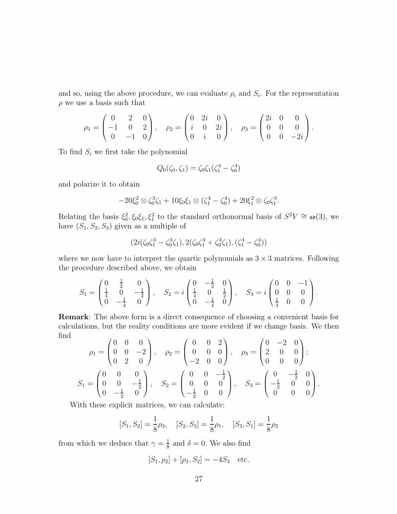
and so, using the above procedure, we can evaluate ρi and Si. For the representationρ we use a basis such that
ρ1 =
0 2 0−1 0 20 −1 0
, ρ2 =
0 2i 0i 0 2i0 i 0
, ρ3 =
2i 0 00 0 00 0 −2i
.
To find Si we first take the polynomial
Q6(ζ0, ζ1) = ζ0ζ1(ζ41 − ζ40)
and polarize it to obtain
−20ξ20 ⊗ ζ30ζ1 + 10ξ0ξ1 ⊗ (ζ41 − ζ40) + 20ξ21 ⊗ ζ0ζ31 .
Relating the basis ξ20 , ξ0ξ1, ξ21 to the standard orthonormal basis of S2V ∼= so(3), we
have (S1, S2, S3) given as a multiple of
(2i(ζ0ζ31 − ζ30ζ1), 2(ζ0ζ
31 + ζ30ζ1), (ζ
41 − ζ40 ))
where we now have to interpret the quartic polynomials as 3× 3 matrices. Followingthe procedure described above, we obtain
S1 =
0 1
20
14
0 −12
0 −14
0
, S2 = i
0 −1
20
14
0 12
0 −14
0
, S3 = i
0 0 −10 0 014
0 0
.
Remark: The above form is a direct consequence of choosing a convenient basis forcalculations, but the reality conditions are more evident if we change basis. We thenfind
ρ1 =
0 0 00 0 −20 2 0
, ρ2 =
0 0 20 0 0−2 0 0
, ρ3 =
0 −2 02 0 00 0 0
;
S1 =
0 0 00 0 −1
2
0 −12
0
, S2 =
0 0 −12
0 0 0−1
20 0
, S3 =
0 −12
0−1
20 0
0 0 0
.
With these explicit matrices, we can calculate:
[S1, S2] =1
8ρ3, [S2, S3] =
1
8ρ1, [S3, S1] =
1
8ρ2
from which we deduce that γ = 18and δ = 0. We also find
[S1, ρ2] + [ρ1, S2] = −4S3 etc.
27
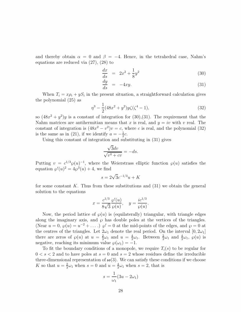
and thereby obtain α = 0 and β = −4. Hence, in the tetrahedral case, Nahm’sequations are reduced via (27), (28) to
dx
ds= 2x2 +
1
8y2 (30)
dy
ds= −4xy. (31)
When Ti = xρi + ySi in the present situation, a straightforward calculation givesthe polynomial (25) as
η3 − 1
2(48x2 + y2)yζ(ζ4 − 1), (32)
so (48x2 + y2)y is a constant of integration for (30),(31). The requirement that theNahm matrices are antihermitian means that x is real, and y = iv with v real. Theconstant of integration is (48x2 − v2)v = c, where c is real, and the polynomial (32)is the same as in (21), if we identify a = −1
2c.
Using this constant of integration and substituting in (31) gives√3dv√
v4 + cv= −ds.
Putting v = c1/3℘(u)−1, where the Weierstrass elliptic function ℘(u) satisfies theequation ℘′(u)2 = 4℘3(u) + 4, we find
s = 2√3c−1/3u+K
for some constant K. Thus from these substitutions and (31) we obtain the generalsolution to the equations
x =c1/3
8√3
℘′(u)
℘(u), y =
ic1/3
℘(u).
Now, the period lattice of ℘(u) is (equilaterally) triangular, with triangle edgesalong the imaginary axis, and ℘ has double poles at the vertices of the triangles.(Near u = 0, ℘(u) = u−2 + . . . .) ℘′ = 0 at the mid-points of the edges, and ℘ = 0 atthe centres of the triangles. Let 2ω1 denote the real period. On the interval [0, 2ω1]there are zeros of ℘(u) at u = 2
3ω1 and u = 4
3ω1. Between 2
3ω1 and 4
3ω1, ℘(u) is
negative, reaching its minimum value ℘(ω1) = −1.To fit the boundary conditions of a monopole, we require Ti(s) to be regular for
0 < s < 2 and to have poles at s = 0 and s = 2 whose residues define the irreduciblethree-dimensional representation of so(3). We can satisfy these conditions if we chooseK so that u = 2
3ω1 when s = 0 and u = 4
3ω1 when s = 2, that is
s =1
ω1
(3u− 2ω1)
28
with 2ω1 =√3c1/3. Both x and y have simple poles at s = 0 and s = 2, and
one can verify that the residues of the Nahm matrices there define an irreduciblerepresentation of so(3). Moreover, x and y have no singularities for 0 < s < 2. Sincey(2− s) = y(s) and x(2− s) = −x(s), it follows that Ti(2− s) = Ti(s)
T .It is straightforward to see that another solution with these boundary conditions
is obtained by replacing 2ω1 by −2ω1; the result is a reflection of the monopole aboutthe origin.
Yet another solution of Nahm’s equations is obtained by choosing K = 0, withu = 2
3ω1 at s = 2. This gives an equivalent monopole, with the same spectral curve.
Although the symmetry s → 2 − s is no longer manifest, it can be obtained after aunitary transformation of the matrices.
The elliptic curve featured in the solution is a very special one, and the period2ω1 may be evaluated explicitly. We have (see e.g. [27])
2ω1 =∫ ∞
−1
dt√t3 + 1
=1
2√πΓ(
1
6)Γ(
1
3)
and consequently
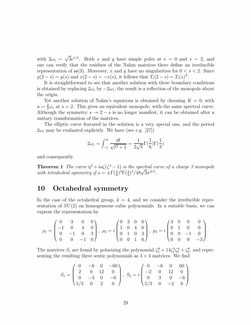
Theorem 1 The curve η3 + iaζ(ζ4 − 1) is the spectral curve of a charge 3 monopolewith tetrahedral symmetry if a = ±Γ(1
6)3Γ(1
3)3/48
√3π3/2.
10 Octahedral symmetry
In the case of the octahedral group, k = 4, and we consider the irreducible repre-sentation of SU(2) on homogeneous cubic polynomials. In a suitable basis, we canexpress the representation by
ρ1 =
0 3 0 0−1 0 4 00 −1 0 30 0 −1 0
, ρ2 = i
0 3 0 01 0 4 00 1 0 30 0 1 0
, ρ3 = i
3 0 0 00 1 0 00 0 −1 00 0 0 −3
.
The matrices Si are found by polarizing the polynomial ζ81 + 14ζ41ζ40 + ζ80 , and repre-
senting the resulting three sextic polynomials as 4× 4 matrices. We find
S1 =
0 −6 0 −602 0 12 00 −3 0 −65/3 0 2 0
, S2 = i
0 −6 0 60−2 0 12 00 3 0 −65/3 0 −2 0
29
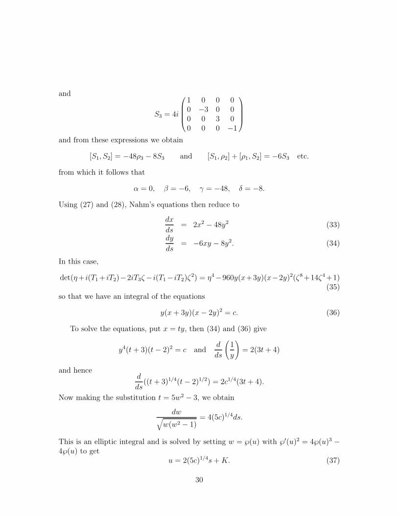
and
S3 = 4i
1 0 0 00 −3 0 00 0 3 00 0 0 −1
and from these expressions we obtain
[S1, S2] = −48ρ3 − 8S3 and [S1, ρ2] + [ρ1, S2] = −6S3 etc.
from which it follows that
α = 0, β = −6, γ = −48, δ = −8.
Using (27) and (28), Nahm’s equations then reduce to
dx
ds= 2x2 − 48y2 (33)
dy
ds= −6xy − 8y2. (34)
In this case,
det(η+ i(T1+ iT2)−2iT3ζ− i(T1− iT2)ζ2) = η4−960y(x+3y)(x−2y)2(ζ8+14ζ4+1)
(35)so that we have an integral of the equations
y(x+ 3y)(x− 2y)2 = c. (36)
To solve the equations, put x = ty, then (34) and (36) give
y4(t+ 3)(t− 2)2 = c andd
ds
(1
y
)= 2(3t+ 4)
and henced
ds((t+ 3)1/4(t− 2)1/2) = 2c1/4(3t+ 4).
Now making the substitution t = 5w2 − 3, we obtain
dw√w(w2 − 1)
= 4(5c)1/4ds.
This is an elliptic integral and is solved by setting w = ℘(u) with ℘′(u)2 = 4℘(u)3 −4℘(u) to get
u = 2(5c)1/4s+K. (37)
30
The general solution to the equation is then
x =2c1/4(5℘2(u)− 3)
53/4℘′(u), y =
2c1/4
53/4℘′(u).
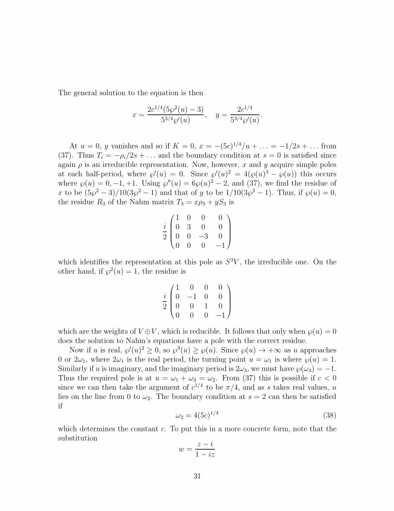
At u = 0, y vanishes and so if K = 0, x = −(5c)1/4/u + . . . = −1/2s + . . . from(37). Thus Ti = −ρi/2s + . . . and the boundary condition at s = 0 is satisfied sinceagain ρ is an irreducible representation. Now, however, x and y acquire simple polesat each half-period, where ℘′(u) = 0. Since ℘′(u)2 = 4(℘(u)3 − ℘(u)) this occurswhere ℘(u) = 0,−1,+1. Using ℘′′(u) = 6℘(u)2 − 2, and (37), we find the residue ofx to be (5℘2 − 3)/10(3℘2 − 1) and that of y to be 1/10(3℘2 − 1). Thus, if ℘(u) = 0,the residue R3 of the Nahm matrix T3 = xρ3 + yS3 is
i
2
1 0 0 00 3 0 00 0 −3 00 0 0 −1
which identifies the representation at this pole as S3V , the irreducible one. On theother hand, if ℘2(u) = 1, the residue is
i
2
1 0 0 00 −1 0 00 0 1 00 0 0 −1
which are the weights of V ⊕V , which is reducible. It follows that only when ℘(u) = 0does the solution to Nahm’s equations have a pole with the correct residue.
Now if u is real, ℘′(u)2 ≥ 0, so ℘3(u) ≥ ℘(u). Since ℘(u) → +∞ as u approaches0 or 2ω1, where 2ω1 is the real period, the turning point u = ω1 is where ℘(u) = 1.Similarly if u is imaginary, and the imaginary period is 2ω3, we must have ℘(ω3) = −1.Thus the required pole is at u = ω1 + ω3 = ω2. From (37) this is possible if c < 0since we can then take the argument of c1/4 to be π/4, and as s takes real values, ulies on the line from 0 to ω2. The boundary condition at s = 2 can then be satisfiedif
ω2 = 4(5c)1/4 (38)
which determines the constant c. To put this in a more concrete form, note that thesubstitution
w =z − i
1− iz
31
transforms the differential
du =℘′du√
4(℘3 − ℘)=
dw
2√w3 − w
into
(1 + i)dz
2√z4 − 1
and so
ω2 = (1 + i)∫ 1
0
dt√1− t4
.
From [27], we also have the formula
∫ 1
0
dt√1− t4
=1√8π
Γ(1
4)2.
Using this, together with (38) and (35), we obtain
Theorem 2 The curve η4 + a(ζ8 + 14ζ4 + 1) is the spectral curve of a charge 4monopole with octahedral symmetry if a = 3Γ(1
4)8/64π2.
11 Icosahedral symmetry
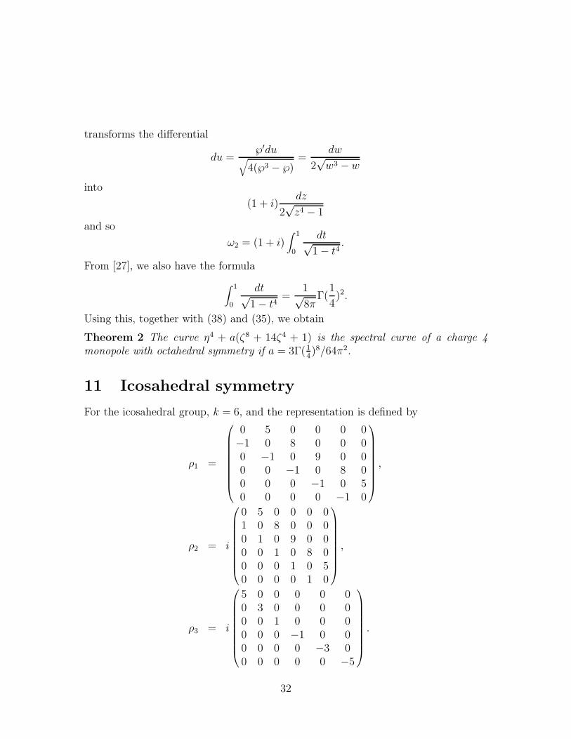
For the icosahedral group, k = 6, and the representation is defined by
ρ1 =
0 5 0 0 0 0−1 0 8 0 0 00 −1 0 9 0 00 0 −1 0 8 00 0 0 −1 0 50 0 0 0 −1 0
,
ρ2 = i
0 5 0 0 0 01 0 8 0 0 00 1 0 9 0 00 0 1 0 8 00 0 0 1 0 50 0 0 0 1 0
,
ρ3 = i
5 0 0 0 0 00 3 0 0 0 00 0 1 0 0 00 0 0 −1 0 00 0 0 0 −3 00 0 0 0 0 −5
.
32
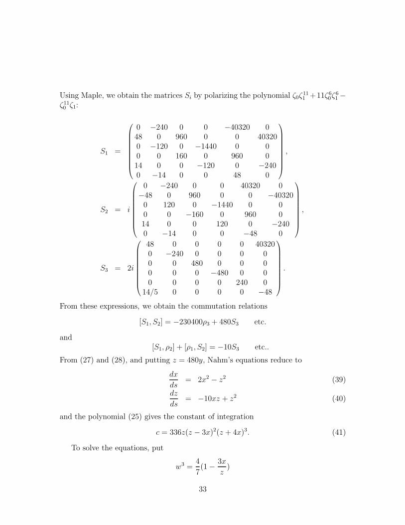
Using Maple, we obtain the matrices Si by polarizing the polynomial ζ0ζ111 +11ζ60ζ
61 −
ζ110 ζ1:
S1 =
0 −240 0 0 −40320 048 0 960 0 0 403200 −120 0 −1440 0 00 0 160 0 960 014 0 0 −120 0 −2400 −14 0 0 48 0
,
S2 = i
0 −240 0 0 40320 0−48 0 960 0 0 −403200 120 0 −1440 0 00 0 −160 0 960 014 0 0 120 0 −2400 −14 0 0 −48 0
,
S3 = 2i
48 0 0 0 0 403200 −240 0 0 0 00 0 480 0 0 00 0 0 −480 0 00 0 0 0 240 0
14/5 0 0 0 0 −48
.
From these expressions, we obtain the commutation relations
[S1, S2] = −230400ρ3 + 480S3 etc.
and[S1, ρ2] + [ρ1, S2] = −10S3 etc..
From (27) and (28), and putting z = 480y, Nahm’s equations reduce to
dx
ds= 2x2 − z2 (39)
dz
ds= −10xz + z2 (40)
and the polynomial (25) gives the constant of integration
c = 336z(z − 3x)2(z + 4x)3. (41)
To solve the equations, put
w3 =4
7(1− 3x
z)
33
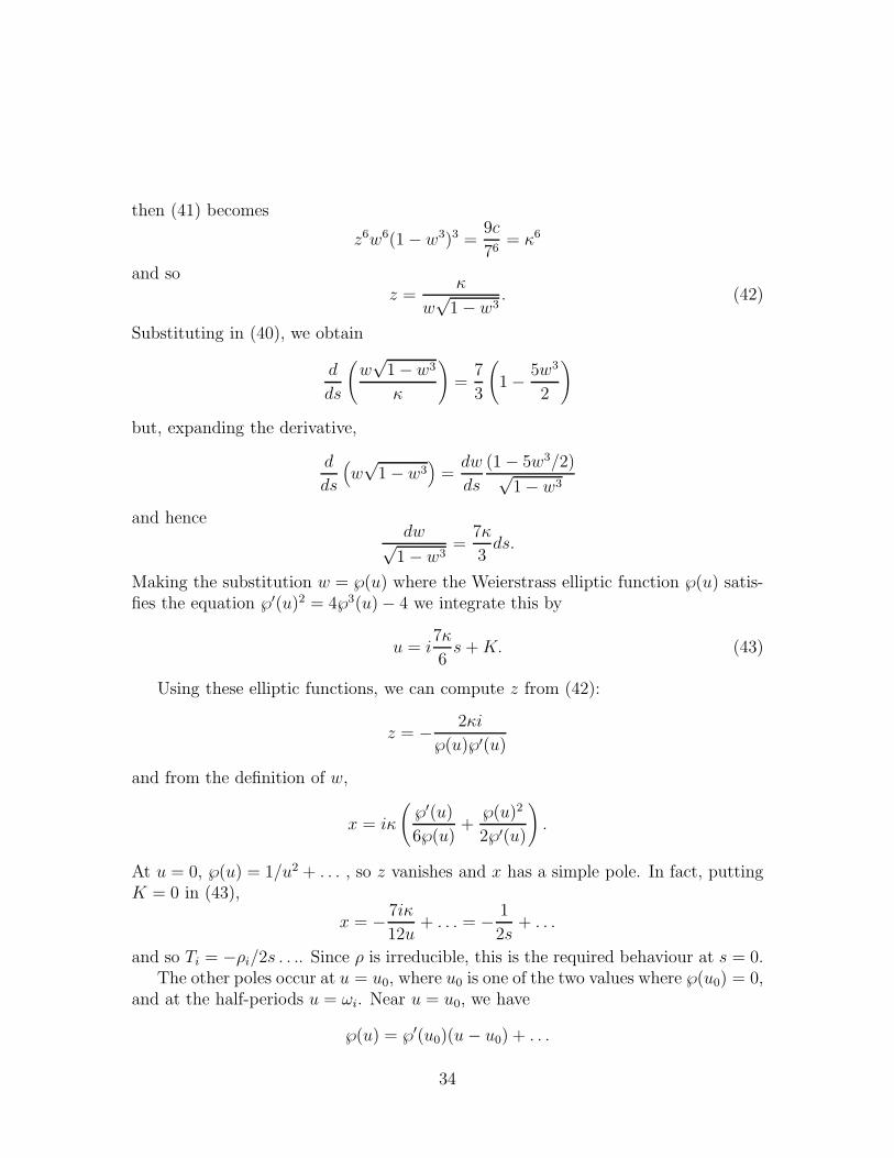
then (41) becomes
z6w6(1− w3)3 =9c
76= κ6
and soz =
κ
w√1− w3
. (42)
Substituting in (40), we obtain
d
ds
(w√1− w3
κ
)=
7
3
(1− 5w3
2
)
but, expanding the derivative,
d
ds
(w√1− w3
)=
dw
ds
(1− 5w3/2)√1− w3
and hencedw√1− w3
=7κ
3ds.
Making the substitution w = ℘(u) where the Weierstrass elliptic function ℘(u) satis-fies the equation ℘′(u)2 = 4℘3(u)− 4 we integrate this by
u = i7κ
6s +K. (43)
Using these elliptic functions, we can compute z from (42):
z = − 2κi
℘(u)℘′(u)
and from the definition of w,
x = iκ
(℘′(u)
6℘(u)+
℘(u)2
2℘′(u)
).
At u = 0, ℘(u) = 1/u2 + . . . , so z vanishes and x has a simple pole. In fact, puttingK = 0 in (43),
x = − 7iκ
12u+ . . . = − 1
2s+ . . .
and so Ti = −ρi/2s . . .. Since ρ is irreducible, this is the required behaviour at s = 0.The other poles occur at u = u0, where u0 is one of the two values where ℘(u0) = 0,
and at the half-periods u = ωi. Near u = u0, we have
℘(u) = ℘′(u0)(u− u0) + . . .
34
and since ℘′(u)2 = 4℘(u)3 − 4, we obtain
x =iκ
6(u− u0)+ . . . =
1
7(s− s0)+ . . .
and
z =iκ
2(u− u0)+ . . . =
3
7(s− s0)+ . . .
using (43). Using this, we calculate the residues Ri of the matrices Ti = xρi+ySi andfind the eigenvalues of iR3 to be −1,−1, 0, 0, 1, 1, thus identifying the representationas S2V ⊕ S2V . At a half-period ωi,
℘(u) = ℘(ωi) + ℘′′(ωi)(u− ωi)2/2 + . . .
but since ℘′(u)2 = 4℘(u)3 − 4, ℘′′(ωi) = 6℘(ωi)2 and this provides x(s) with a
simple pole of residue 1/14 and z a simple pole of residue −2/7 at the correspondingvalue of s. The eigenvalues of iR3 are then −1/2,−1/2,−1/2, 1/2, 1/2, 1/2, givingthe representation V ⊕ V ⊕ V .
It follows that only the poles at the period points give irreducible representations.But any line joining two periods passes through a half-period. We conclude that thereis no solution to Nahm’s equations of this form which is smooth in the interval (0, 2),has poles at the end-points, and whose residues give an irreducible representation.Consequently
Theorem 3 There does not exist a monopole of charge 6 with icosahedral symmetry.
12 Cyclically symmetric scattering of monopoles
In this Section, we shall investigate the rational maps of monopoles with cyclic sym-metry, and shall discover some novel types of geodesic monopole scattering. Recallthat there is a 1 − 1 correspondence between the maps and monopoles. Also, cyclicor axial symmetry about the x3-axis, if present, is manifest.
The rational map of a charge k monopole takes the form
R(z) =p(z)
q(z),
with q monic of degree k and p of degree less than k. Let ω = e2πi/k. Considerthe cyclic group of rotations about the x3-axis, Ck, generated by the transformationz → ωz. The monopole with rational map R(z) is Ck symmetric if R(ωz) differs
35
from R(z) only by a constant phase. We get a class of charge k monopoles with Ck
symmetry for each irreducible character of Ck. Let us denote the lth such class ofmonopoles by M l
k (0 ≤ l < k). These are the monopoles whose rational maps are ofthe form
R(z) =µzl
zk − ν
where µ and ν are complex parameters. For these monopoles, R(ωz) = ωlR(z). M lk
is a 4-dimensional totally geodesic submanifold of the moduli space Mk, since it arisesby imposing a symmetry on the monopoles. Its metric is also Kahler, because the setof rational maps M l
k is a complex submanifold of the set of all rational maps.Since the strongly centred monopoles are geodesic in the moduli space, we shall
now restrict attention to rational maps of strongly centred, Ck-symmetric monopoles.There is no essential loss of generality in doing this. For a monopole with a rationalmap of type M l
k, the criterion for it to be strongly centred (12), reduces to
µkk∏
i=1
(βi)l = 1 (44)
where {βi : i = 1, . . . , k} are the k roots of zk − ν = 0. Eq. (44) is equivalent toµkνl = ±1, with the lower sign if both k is even and l odd, and the upper signotherwise. The magnitude of µ is |µ| = |ν|−l/k, and there are k choices for the phaseof µ. The rational maps we obtain are parametrised by several surfaces of revolution.For given k and l there may be one or more surfaces. For l = 0, for example, thereare k distinct surfaces, each with ν a good coordinate; µ is a distinct, and constant,kth root of unity on each surface. If l 6= 0, and k and l have highest common factorh, there are h distinct surfaces. As arg ν increases by 2π, arg µ decreases by 2πl/k,so arg ν must increase by 2πk/h for µ to return to its initial value. ν is therefore agood coordinate on each surface, but the range of arg ν is 2πk/h.
For given k, and each l in the range 0 ≤ l < k, let us choose one of the surfaces justdescribed, say, the one containing the rational map in M l
k with ν = 1 and µ = eπi/k
(if k is even and l odd) or µ = 1 (otherwise). Denote this surface by Σlk. If there is
another surface, for a particular value of l, then it is isomorphic to Σlk, as µ differs
on it simply by a constant phase. Let us now consider the geodesics on Σlk, and
the associated Ck-symmetric monopole scattering. The simplest geodesic is when νmoves along the real axis – the monopole then has no angular momentum.
On Σ0k the rational maps are of the form
R(z) =1
zk − ν,
where ν is an arbitrary complex number. Σ0k is therefore a submanifold of the space
of inversion symmetric monopoles IM0k . For ν = 0, the rational map is that of a
36
strongly centred axisymmetric charge k monopole. If |ν| is large, there are k well-separated unit charge monopoles at the vertices of an k-gon in R3, with x1 + ix2 akth root of ν, and x3 = 0. The geodesic where ν moves along the entire real axiscorresponds to a simultaneous scattering of k unit charge monopoles in the (x1, x2)plane, where the incoming and outgoing trajectories are related by a π/k rotation.The configuration is instantaneously axially symmetric when ν = 0. This kind ofsymmetric planar scattering of k solitons has been observed in a number of models,and can be understood in a rather general way [17, 8].
On Σlk, with l 6= 0, ν is a non-zero complex number. ν = 0 is forbidden, as
the numerator and denominator of R(z) would have a common factor zl. A simplegeodesic is with ν moving along the positive real axis, say towards ν = 0. The rationalmap is
R(z) =ι
νl/k
zl
zk − ν(45)
where ι = eπi/k (if k is even and l is odd) or ι = 1 (otherwise). Then the initialmotion is again k unit charge monopoles at the vertices of a contracting k-gon in the(x1, x2) plane. As ν → 0, the map approaches
R(z) =ι
νl/k
1
zk−l
which is the map of a charge (k − l) axisymmetric monopole, centred at the point(0, 0, (−l/2k) log ν). This is a positive distance along the x3-axis as ν is small. Fol-lowing an argument in [[1], pp.25-6], we deduce that the charge k monopole has splitup, with one cluster the charge k − l monopole just described, and a further cluster(or clusters) near the x3-axis, but not so far up. In fact, there is just one other cluster,which is an axisymmetric charge l monopole at a negative distance along the x3-axis.This is seen by inverting the original monopole in the (x1, x2) plane. The proceduredescribed in Section 4 shows that the rational map (45) transforms under inversionto
R(z) =ι
ν(k−l)/k
zk−l
zk − ν
where ι ι = 1, because
ι ι (zl/νl/k) (zk−l/ν(k−l)/k) = zk/ν= 1 mod zk − ν.
The inverted monopole therefore has an axisymmetric charge l monopole cluster at(0, 0,−((k−l)/2k) log ν), as ν → 0, while the original monopole has this axisymmetriccharge l cluster at (0, 0, ((k − l)/2k) log ν).
37
In the geodesic motion, k unit charge monopoles come in, but the outgoing con-figuration is of two approximately axisymmetric monopole clusters, of charges k − land l, at distances ld and −(k − l)d along the x3-axis, with d increasing uniformly.This geodesic motion can, of course, also be reversed. The centre of mass of theseclusters remains at the origin.
If k is even and l = k/2 then the rational maps, and the geodesic monopole motionwe have described, have an additional inversion symmetry. R(z) = zk/2/(ν1/2(zk−ν))
lies in the space of inversion symmetric maps IMk/2k , and the factor ι makes no
essential difference. Consequently, the outgoing clusters have the same charges andequal speeds. Since ν was assumed to be real, there is reflection symmetry underx2 → −x2. Together with the inversion symmetry, x3 → −x3, we obtain an additionalrotational symmetry, by π about the x1-axis. Hence, monopoles with rational maps ofthe form (45) have Dk symmetry if k is even and l = k/2. There is also Dk symmetryif l = 0, for any k.
The surfaces Σ02 and Σ1
2 are the “rounded cone” and “trumpet” described in [1].These surfaces are not isomorphic, but the geodesics with ν real (on Σ0
2) and ν realand positive (on Σ1
2) are isomorphic. Along the first, two unit charge monopolesscatter through π/2 in the (x1, x2) plane, and along the second they scatter throughπ/2 in the (x1, x3) plane. There are no analogous isomorphisms in the higher chargecases.
The general geodesics on the surfaces Σ0k and Σl
k (l 6= 0) are presumably analogousto those on the cone Σ0
2 or trumpet Σ12. On Σ0
k, they correspond to k unit chargemonopoles scattering in the (x1, x2) plane with net orbital angular momentum. OnΣl
k (l 6= 0), k unit charge monopoles again come in with net orbital angular momen-tum. If this is small, the geodesic passes through the trumpet-like surface and twomonopole clusters with magnetic charges l and k − l emerge back-to-back on the x3-axis. They also have opposite electric charges, which accounts, physically, for angularmomentum conservation. If the initial angular momentum is large, then the geodesicdoes not pass through the trumpet, but is reflected, and there are k outgoing unitcharge monopoles in the (x1, x2) plane.
What can we learn about the spectral curves of centred Ck-symmetric monopolesfrom this discussion of rational maps? First, recall that monopoles whose rationalmaps differ only by a phase have the same spectral curves. We need therefore onlyconsider the chosen surfaces of rational maps, Σl
k, and their associated monopoles. Letus also restrict attention to monopoles which are oriented to be reflection symmetricunder x2 → −x2, which requires ν to be real, and choose a fixed phase for µ as νvaries in magnitude. This restricts us to 2k − 1 disjoint curves in the surfaces Σl
k, (νreal in Σ0
k, ν positive and ν negative in Σlk (l 6= 0)), and these curves are geodesics. It
follows that among the centred curves in TP1 of the form (5) with Ck symmetry and
38
oriented, there are 2k−1 disjoint loci of spectral curves. (We refer to a connected, one-dimensional submanifold of spectral curves as a locus in the space of curves in TP1.)All these spectral curves will have real coefficients because of the reflection symmetry.We have been unable to determine, in general, for which parameter values a curve isa spectral curve, but we can make some qualitative assertions, based on knowledgeof the asymptotic monopole configurations, the axisymmetric configurations, and themonopoles with the symmetries of the regular solids. We restrict our remarks to thecases k = 3 and k = 4.
For k = 3, and l = 0, 1 or 2, there are five loci of spectral curves of the form (17),with β real. When l = 0 there is D3-symmetry, so γ = 0. The locus is asymptotic atboth ends to α3 = 27β2, with β large and positive at one end, and β large and negativeat the other. The axisymmetric monopole, half-way along the locus, has β = 0 andα = π2. Presumably, α is positive along the whole locus. The four remaining loci, forl = 1 and l = 2, are isomorphic. This is because ν → −ν corresponds to a reflectionx1 → −x1, and because the l = 2 monopoles are obtained from l = 1 monopoles byinversion (x3 → −x3). Under the first symmetry β → −β, and under the secondγ → −γ. Each of the four loci is asymptotic at one end to α3 = 27β2, γ = 0, with βeither positive or negative, and at the other to α = 1
4π2−3b2, β = 0, γ = 2b(b2+ 1
4π2),
with b either positive or negative. These latter parameters result from taking theproduct of the spectral curve of a unit charge monopole at (0, 0, b) with the spectralcurve of an axisymmetric charge 2 monopole at (0, 0,−b/2), that is
P (η, ζ) = (η + 2bζ)(η2 − 2bηζ + (b2 + 14π2)ζ2)
= η3 + (14π2 − 3b2)ηζ2 + 2b(b2 + 1
4π2)ζ3 = 0.
Since the tetrahedrally symmetric charge 3 monopole has C3 symmetry about variousaxes, there must be a point on each of these four loci corresponding to such a monopole(in four distinct orientations). The calculations of Section 9 show that the four locipass through the four points (one on each locus) (α, β, γ) = (0,±a,±5
√2a), where
a = Γ(16)3Γ(1
3)3/48
√3π3/2. The picture of the monopole scattering, corresponding to
geodesic motion along one of these loci, is as follows. Three unit charge monopolescome in at the vertices of a (horizontal) equilateral triangle, moving towards itscentre. They then coalesce instantaneously into a tetrahedron, with the base triangleoriented the same way as the initial triangle, but somewhat below the initial plane.Finally the tetrahedron breaks up with the top vertex moving up and becoming a unitcharge monopole, and the base triangle descending and becoming a toroidal chargetwo monopole.
In the case k = 4, we have seven loci of spectral curves with C4 symmetry. Onlythree of these are essentially different. The four corresponding to the rational mapswith l = 1 and l = 3, and ν positive or negative, are isomorphic. The l = 1 andl = 3 maps, and hence the corresponding monopoles and spectral curves, are related
39
by inversion, and the sign of ν can be reversed by a π/4 rotation. The spectral curvesalong these four loci have no higher symmetry than C4 symmetry.
There are two isomorphic loci of spectral curves corresponding to the l = 2 maps.Here there is inversion symmetry, and the spectral curves are therefore D4 symmetricand of the form (19). Reversing the sign of ν again corresponds to a π/4 rotation, andβ changes sign. Along these two loci, we will find the spectral curves corresponding tothe octahedrally symmetric 4-monopole (in two orientations). The locus with ν neg-ative interpolates between the asymptotic parameter values α = 4a2, β = a4, γ = 2a4
with a large (corresponding to four stars at (1/√2)(± a,± a, 0) and the asymptotic
values α = 12π2 − 8b2, β = 0, γ = (4b2 + 1
4π2)2 with b large (corresponding to two
axisymmetric charge 2 monopole clusters on the x3-axis). Along the locus, α changessign, and when α = 0 the locus passes through the spectral curve of the monopolewith octahedral symmetry, so γ = 14β = 21Γ(1
4)8/32π2.
Finally, there is a single locus corresponding to the l = 0 maps. This interpolatesbetween the asymptotic parameter values α = 4a2, β = −a4, γ = 2a4 and α =4a2, β = a4, γ = 2a4, with a large, and passes through the values α = 5π2/2, β =0, γ = 9π4/16, corresponding to the axisymmetric charge 4 monopole. Presumably,α and γ are positive along the entire locus.
In summary, our main result is that in the geodesic scattering of monopoles ofcharge k, with Ck symmetry and angular momentum zero, there are two kinds ofmotion. First, there is the well-known possibility of k monopoles, of unit charge,scattering in the (x1, x2) plane through an angle π/k. Second, there is the novelpossibility of k unit charge monopoles coming in as before, but emerging as charge land charge k − l axisymmetric monopoles moving back-to-back along the x3-axis. lcan have any integer value in the range 0 < l < k. In the special case of 3-monopolescattering, with l = 1 or l = 2, the field configuration passes through the tetrahedrallysymmetric 3-monopole. In 4-monopole scattering, with l = 2, the configuration passesthrough the octahedrally symmetric 4-monopole.
Acknowledgements
N.S.M. warmly thanks the Pure Mathematics Department of the University ofAdelaide and Professor Alan Carey for inviting him to visit, and for financial support.He also thanks the Physics Department of the University of Tasmania at Hobart, andProfessor Delbourgo, for hospitality, and the Royal Society and the British Councilfor travel grants.
M.K.M thanks the Australian Research Council for support and Michael Singerfor useful conversations.
We thank Paul Sutcliffe for help with the analysis of the tetrahedrally symmetricmonopole.
40
References
[1] Atiyah M F and Hitchin N J 1988 The geometry and dynamics of magneticmonopoles (Princeton, NJ: Princeton University Press)
[2] Atiyah M F and Manton N S 1989 Skyrmions from instantons Phys. Lett. 222B438; 1993 Geometry and kinematics of two Skyrmions Commun. Math. Phys.153 391
[3] Bates L and Montgomery R 1988 Closed geodesics on the space of stable two-monopoles Commun. Math. Phys. 118 635
[4] Bielawski R 1994 Monopoles, particles and rational functions (McMaster Uni-versity preprint)
[5] Bogomolny E B 1976 The stability of classical solutions Sov. J. Nucl. Phys. 24449
[6] Braaten E, Townsend S and Carson L 1990 Novel structure of static multisolitonsolutions in the Skyrme model Phys. Lett. 235B 147
[7] Donaldson S K 1984 Nahm’s equations and the classification of monopoles Com-mun. Math. Phys. 96 387
[8] Dziarmaga J 1994 Head-on collision of n vortices Phys. Rev. D49 5609
[9] Ercolani N and Sinha A 1989 Monopoles and Baker functions Commun. Math.Phys. 125 385
[10] Gibbons G W and Manton N S 1986 Classical and quantum dynamics of BPSmonopoles Nucl. Phys. B274 183
[11] Hitchin N J 1982 Monopoles and geodesics Commun. Math. Phys. 83 579
[12] Hitchin N J 1983 On the construction of monopoles Commun. Math. Phys. 89145
[13] Hitchin N J and Murray M K 1988 Spectral curves and the ADHM methodCommun. Math. Phys. 114 463
[14] Hurtubise J 1985 Monopoles and rational maps: a note on a theorem of Donald-son Commun. Math. Phys. 100 191
[15] Klein F 1913 Lectures on the icosahedron (London: Kegan Paul)
41
[16] Kostant B 1959 The principal 3-dimensional subgroup and the Betti numbers ofa complex simple Lie group Amer. J. Math. 81 973
[17] Kudryavtsev A, Piette B and Zakrzewski W J 1993 π/N scattering in 2 + 1dimensions Phys. Lett. 180A 119
[18] Leese R A and Manton N S 1994 Stable instanton-generated Skyrme fields withbaryon numbers three and four Nucl. Phys. A572 575
[19] Manton N S 1978 Complex structure of monopoles Nucl. Phys. B135 319
[20] Manton N S 1982 A remark on the scattering of BPS monopoles Phys. Lett.110B 54
[21] NahmW 1982 The construction of all self-dual monopoles by the ADHM methodMonopoles in quantum field theory (Proceedings of the monopole meeting, Trieste1981) eds Craigie N S, Goddard P and Nahm W (Singapore: World Scientific)p 87
[22] O’Raifeartaigh L and Rouhani S 1982 Rings of monopoles with discrete axialsymmetry: explicit solution for N = 3 Phys. Lett. 112B 143
[23] Skyrme T R H 1962 A unified field theory of mesons and baryons Nucl. Phys.31 556
[24] Stuart D 1994 The geodesic approximation for the Yang-Mills-Higgs equationsCommun. Math. Phys. 166 149
[25] Taubes C 1980 Arbitrary N -vortex solutions to the first order Ginzburg-Landauequations Commun. Math. Phys. 72 277
[26] Temple-Raston M and Alexander D 1993 Differential cross sections and es-cape plots for low-energy solitonic SU(2) BPS magnetic monopole dynamicsNucl.Phys. B397 195
[27] Whittaker E T and Watson G N 1920 A course in modern analysis (3rd ed)(Cambridge: Cambridge University Press)
[28] Wojtkowski M P 1988 Bounded geodesics for the Atiyah-Hitchin metric Bull.Amer. Math. Soc. 18 179
42