Embed Size (px)
DESCRIPTION
Damping and Modal Analysis
Citation preview
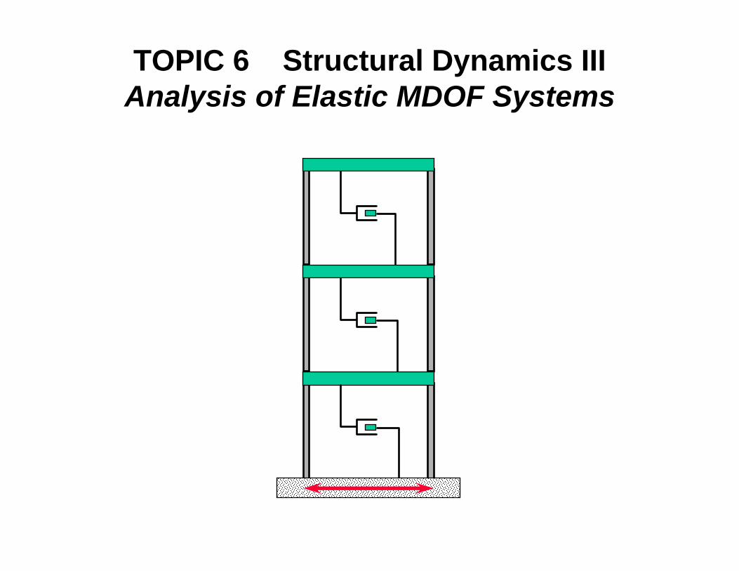
TOPIC 6 Structural Dynamics IIIAnalysis of Elastic MDOF Systems
TOPIC 6 Structural Dynamics IIIAnalysis of Elastic MDOF Systems
• Equations of Motion for MDOF Systems
• Uncoupling of Equations through use of Natural Mode Shapes
• Solution of Uncoupled Equations
• Recombination of Computed Response
• Modal Response Spectrum Analysis (By Example)
• Use of Reduced Number of Modes
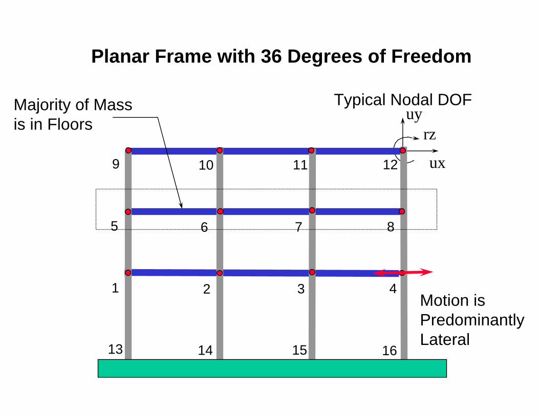
ux
uyrz
Majority of Massis in Floors
Typical Nodal DOF
Motion isPredominantlyLateral
Planar Frame with 36 Degrees of Freedom
1 2 3 4
5 6 7 8
9 10 11 12
13 14 15 16
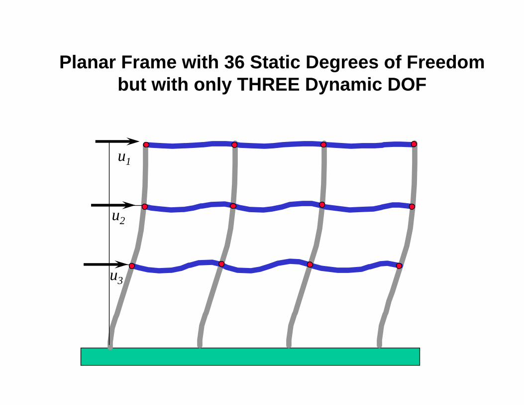
Planar Frame with 36 Static Degrees of Freedombut with only THREE Dynamic DOF
u1
u2
u3
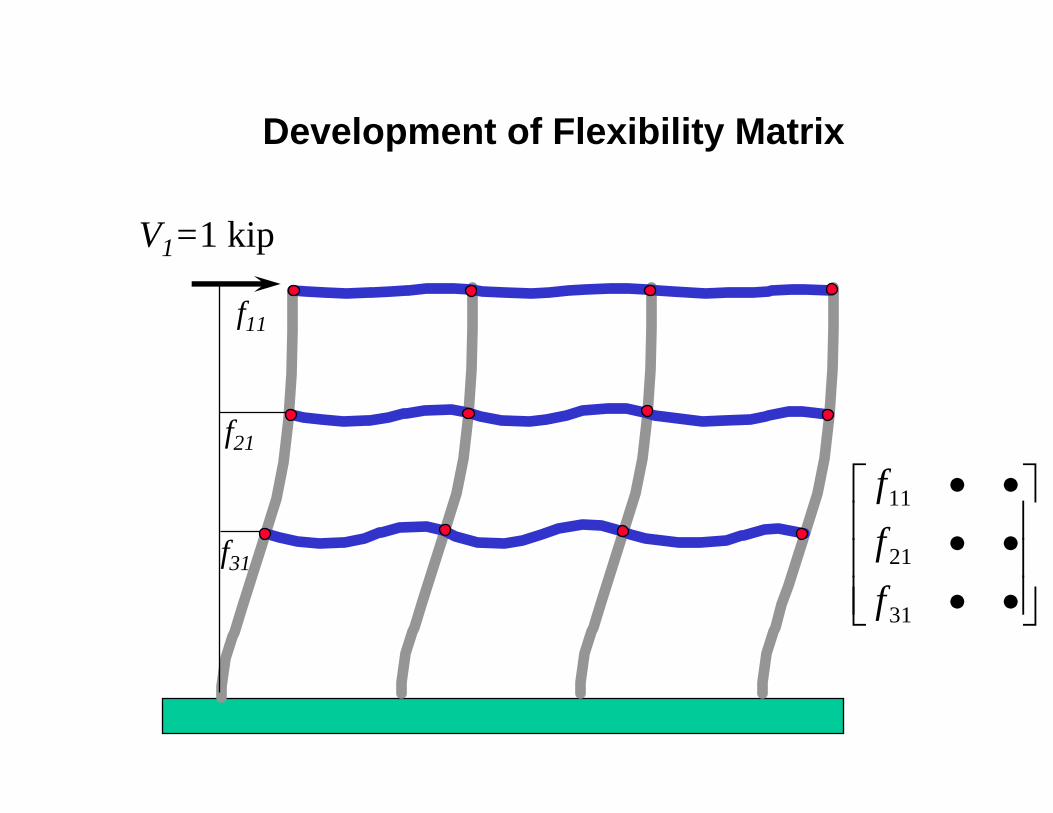
f11
f21
f31
V1=1 kip
fff
11
21
31
• •• •• •
⎡
⎣
⎢⎢⎢
⎤
⎦
⎥⎥⎥
Development of Flexibility Matrix
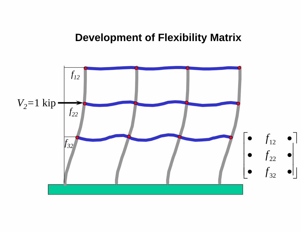
Development of Flexibility Matrix
f12
f22
f32
V2=1 kip
• •• •• •
⎡
⎣
⎢⎢⎢
⎤
⎦
⎥⎥⎥
fff
12
22
32
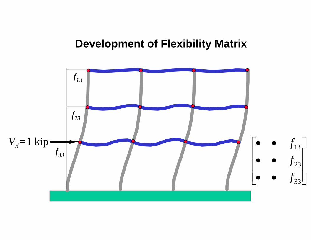
Development of Flexibility Matrix
f13
f23
f33
V3=1 kip • •• •• •
⎡
⎣
⎢⎢⎢
⎤
⎦
⎥⎥⎥
fff
13
23
33
Ufff
Vfff
Vfff
V=⎧
⎨⎪
⎩⎪
⎫
⎬⎪
⎭⎪
+⎧
⎨⎪
⎩⎪
⎫
⎬⎪
⎭⎪
+⎧
⎨⎪
⎩⎪
⎫
⎬⎪
⎭⎪
11
21
31
1
12
22
33
2
13
23
33
3
Uf f ff f ff f f
VVV
=⎡
⎣
⎢⎢⎢
⎤
⎦
⎥⎥⎥
⎧
⎨⎪
⎩⎪
⎫
⎬⎪
⎭⎪
11 12 13
21 22 23
31 32 33
1
2
3
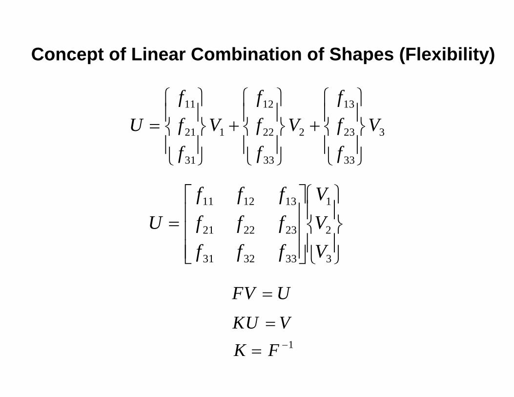
FV U=
KU V=K F= −1
Concept of Linear Combination of Shapes (Flexibility)
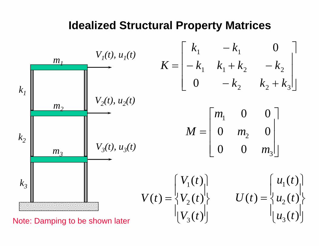
m1
m3
m2
k1
k2
k3
V1(t), u1(t)
V2(t), u2(t)
V3(t), u3(t)
Kk kk k k k
k k k=
−− + −
− +
⎡
⎣
⎢⎢⎢
⎤
⎦
⎥⎥⎥
1 1
1 1 2 2
2 2 3
0
0
Mm
mm
=⎡
⎣
⎢⎢⎢
⎤
⎦
⎥⎥⎥
1
2
3
0 00 00 0
U tu tu tu t
( )( )( )( )
=⎧
⎨⎪
⎩⎪
⎫
⎬⎪
⎭⎪
1
2
3
V tV tV tV t
( )( )( )( )
=⎧
⎨⎪
⎩⎪
⎫
⎬⎪
⎭⎪
1
2
3
Idealized Structural Property Matrices
Note: Damping to be shown later
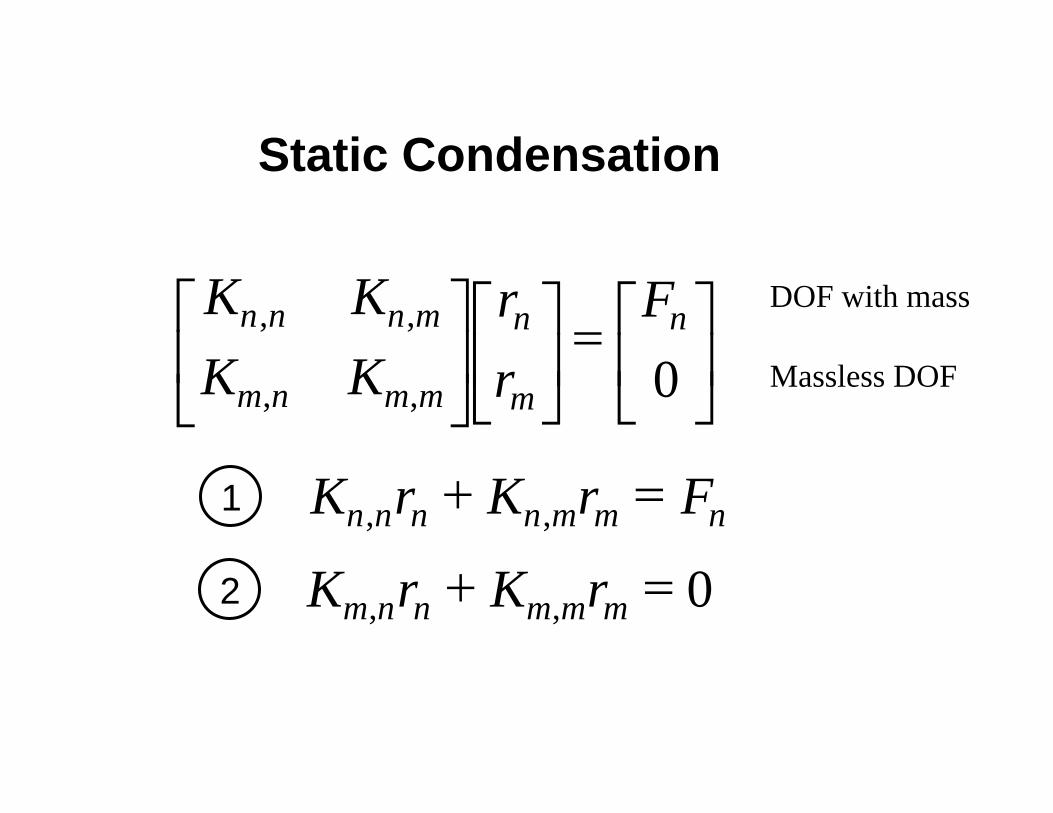
K KK K
rr
Fn n n m
m n m m
n
m
n, ,
, ,
LNM
OQPLNMOQP= LNMOQP
K r K r Fn n n n m m n, ,+ =
0
K r K rm n n m m m, ,+ = 0
Static Condensation
Massless DOF
DOF with mass
2
1
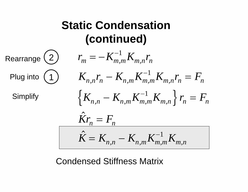
Condensed Stiffness Matrix
Static Condensation(continued)
r K K r
K r K K K r F
K K K K r F
Kr F
K K K K K
m m m m n n
n n n n m m m m n n n
n n n m m m m n n n
n n
n n n m m m m n
= −
− =
− =
=
= −
−
−
−
−
, ,
, , , ,
, , , ,
, , , ,
1
1
1
1
n s
2
1
Rearrange
Plug into
Simplify
m
m
m
u t
u t
u t
k k
k k k k
k k k
u t
u t
u t
V t
V t
V t
1
2
3
1
2
3
1 1
1 1 2 2
2 2 3
1
2
3
1
2
3
0 0
0 0
0 0
0
0
⎡
⎣
⎢⎢⎢
⎤
⎦
⎥⎥⎥
⎧
⎨⎪
⎩⎪
⎫
⎬⎪
⎭⎪+
−
− + −
− +
⎡
⎣
⎢⎢⎢
⎤
⎦
⎥⎥⎥
⎧
⎨⎪
⎩⎪
⎫
⎬⎪
⎭⎪=
⎧
⎨⎪
⎩⎪
⎫
⎬⎪
⎭⎪
( )
( )
( )
( )
( )
( )
( )
( )
( )
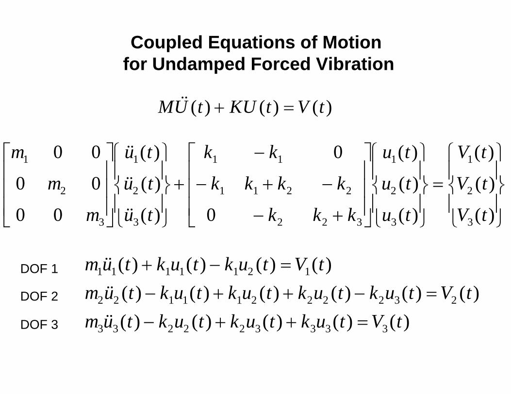
MU t KU t V t( ) ( ) ( )+ =
m u t k u t k u t V tm u t k u t k u t k u t k u t V tm u t k u t k u t k u t V t
1 1 1 1 1 2 1
2 2 1 1 1 2 2 2 2 3 2
3 3 2 2 2 3 3 3 3
( ) ( ) ( ) ( )( ) ( ) ( ) ( ) ( ) ( )( ) ( ) ( ) ( ) ( )
+ − =− + + − =− + + =
Coupled Equations of Motion for Undamped Forced Vibration
DOF 1
DOF 2
DOF 3
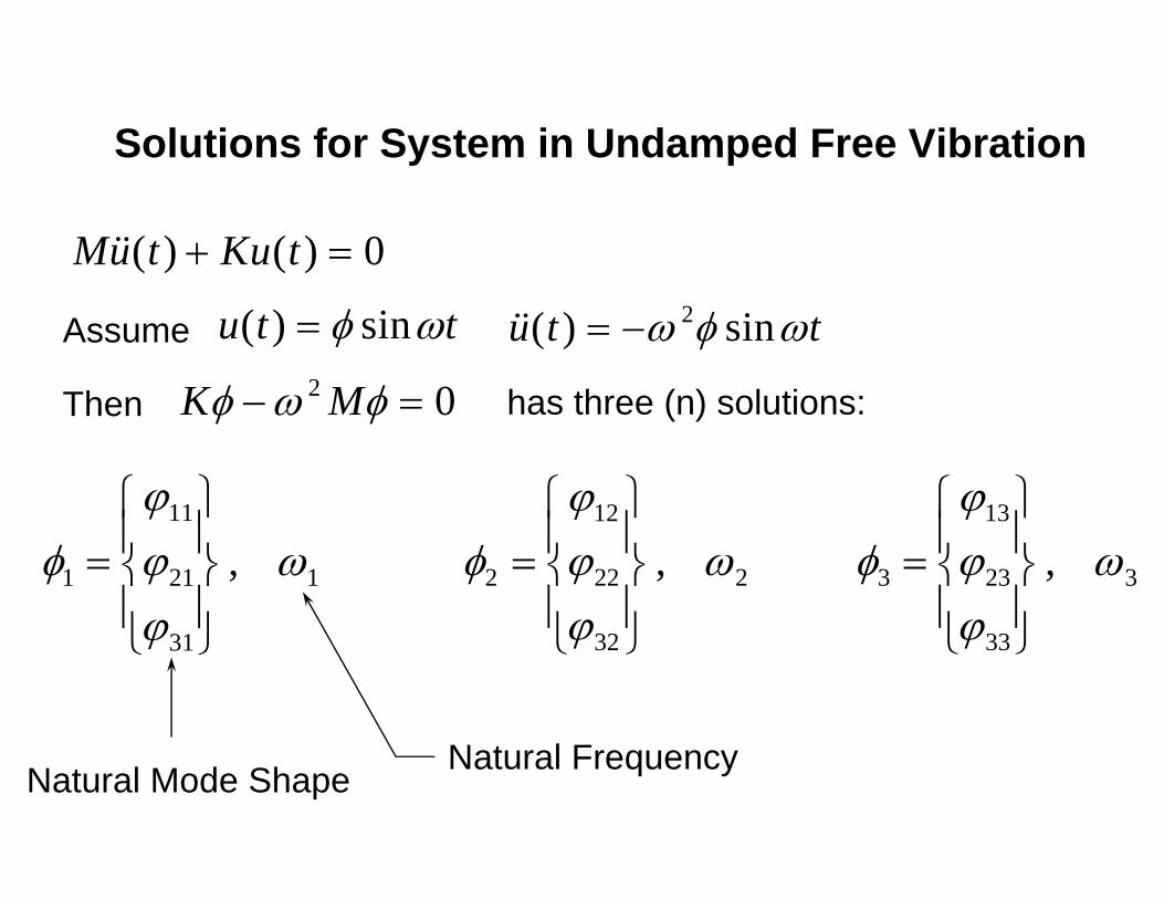
Mu t Ku t( ) ( )+ = 0
Assume u t t( ) sin= φ ω
K Mφ ω φ− =2 0Then has three (n) solutions:
φϕϕϕ
ω1
11
21
31
1=⎧
⎨⎪
⎩⎪
⎫
⎬⎪
⎭⎪
, φϕϕϕ
ω2
12
22
32
2=⎧
⎨⎪
⎩⎪
⎫
⎬⎪
⎭⎪
, φϕϕϕ
ω3
13
23
33
3=⎧
⎨⎪
⎩⎪
⎫
⎬⎪
⎭⎪
,
Natural Mode Shape Natural Frequency
Solutions for System in Undamped Free Vibration
( ) sinu t t= −ω φ ω2
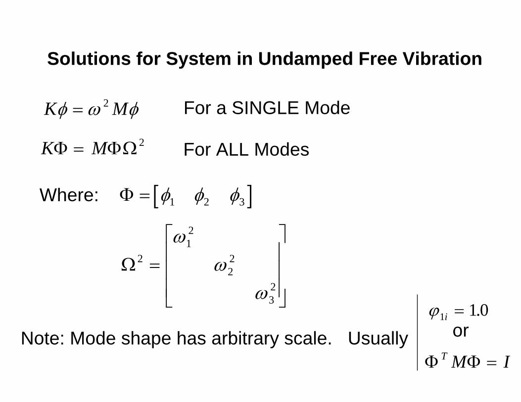
K Mφ ω φ= 2 For a SINGLE Mode
K MΦ ΦΩ= 2 For ALL Modes
[ ]Φ = φ φ φ1 2 3Where:
Ω212
22
32
=
⎡
⎣
⎢⎢⎢
⎤
⎦
⎥⎥⎥
ωω
ω
Solutions for System in Undamped Free Vibration
Note: Mode shape has arbitrary scale. UsuallyΦ ΦT M I=
ϕ1 1 0i = .or
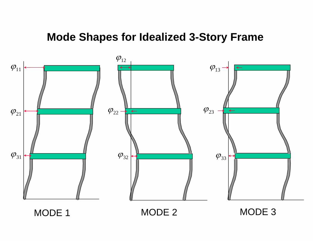
MODE 1 MODE 3MODE 2
ϕ11
ϕ21
ϕ31 ϕ32
ϕ22
ϕ12
ϕ33
ϕ23
ϕ13
Mode Shapes for Idealized 3-Story Frame
U Y Y Y=
⎧
⎨⎪
⎩⎪
⎫
⎬⎪
⎭⎪
+
⎧
⎨⎪
⎩⎪
⎫
⎬⎪
⎭⎪
+
⎧
⎨⎪
⎩⎪
⎫
⎬⎪
⎭⎪
φ
φ
φ
φ
φ
φ
φ
φ
φ
11
21
31
1
12
22
33
2
13
23
33
3U
Y
Y
Y
=
⎡
⎣
⎢⎢⎢
⎤
⎦
⎥⎥⎥
⎧
⎨⎪
⎩⎪
⎫
⎬⎪
⎭⎪
φ φ φ
φ φ φ
φ φ φ
11 12 13
21 22 23
31 32 33
1
2
3
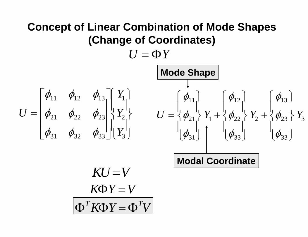
U Y= Φ
KU V=
Concept of Linear Combination of Mode Shapes(Change of Coordinates)
K Y VΦ =Φ Φ ΦT TK Y V=
Mode Shape
Modal Coordinate
[ ]Φ = φ φ φ1 2 3
Φ ΦT Kk
kk
=
⎡
⎣
⎢⎢⎢
⎤
⎦
⎥⎥⎥
1
2
3
*
*
*
Φ ΦT Mm
mm
=
⎡
⎣
⎢⎢⎢
⎤
⎦
⎥⎥⎥
1
2
3
*
*
*
Φ ΦTCc
cc
=
⎡
⎣
⎢⎢⎢
⎤
⎦
⎥⎥⎥
1
2
3
*
*
*
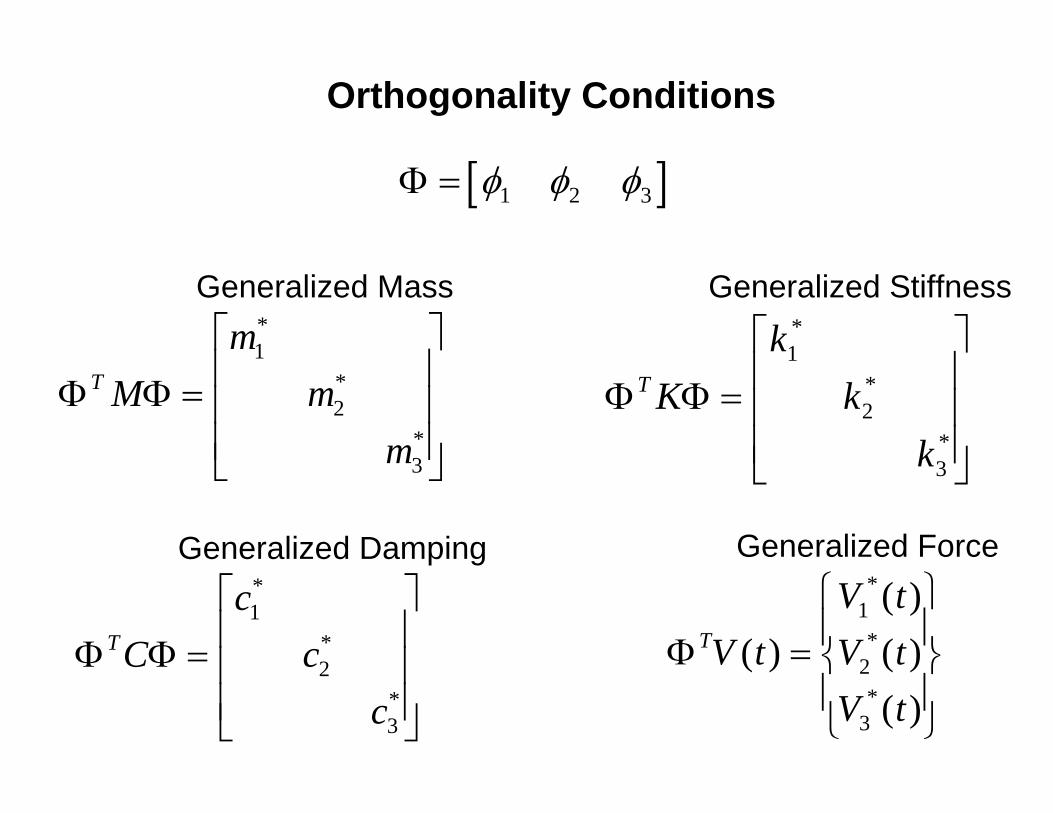
Generalized Mass
Generalized Damping
Generalized Stiffness
Orthogonality Conditions
ΦTV tV tV tV t
( )( )( )( )
*
*
*
=
⎧
⎨⎪
⎩⎪
⎫
⎬⎪
⎭⎪
1
2
3
Generalized Force

Mu Cu Ku V t( )+ + =
yu Φ=M y C y K y V tΦ Φ Φ ( )+ + =
Φ Φ Φ Φ Φ Φ ΦT T T TM y C y K y V t( )+ + =
mm
m
yyy
cc
c
yyy
kk
k
yyy
V tV tV t
1
2
3
1
2
3
1
2
3
1
2
3
1
2
3
1
2
3
1
2
3
*
*
*
*
*
*
*
*
*
*
*
*
( )( )( )
⎡
⎣
⎢⎢⎢
⎤
⎦
⎥⎥⎥
⎧
⎨⎪
⎩⎪
⎫
⎬⎪
⎭⎪+
⎡
⎣
⎢⎢⎢
⎤
⎦
⎥⎥⎥
⎧
⎨⎪
⎩⎪
⎫
⎬⎪
⎭⎪+
⎡
⎣
⎢⎢⎢
⎤
⎦
⎥⎥⎥
⎧
⎨⎪
⎩⎪
⎫
⎬⎪
⎭⎪=
⎧
⎨⎪
⎩⎪
⎫
⎬⎪
⎭⎪
MDOF Equation of Motion:
Transformation of Coordinates:
Substitution:
Premultiply by ΦT:
Using Orthogonality Conditions: Uncoupled Equations of Motion are:
Development of Uncoupled Equations of Motion
ug ,ur 1
⎪⎭
⎪⎬
⎫
⎪⎩
⎪⎨
⎧+
⎪⎭
⎪⎬
⎫
⎪⎩
⎪⎨
⎧
=⎪⎭
⎪⎬
⎫
⎪⎩
⎪⎨
⎧
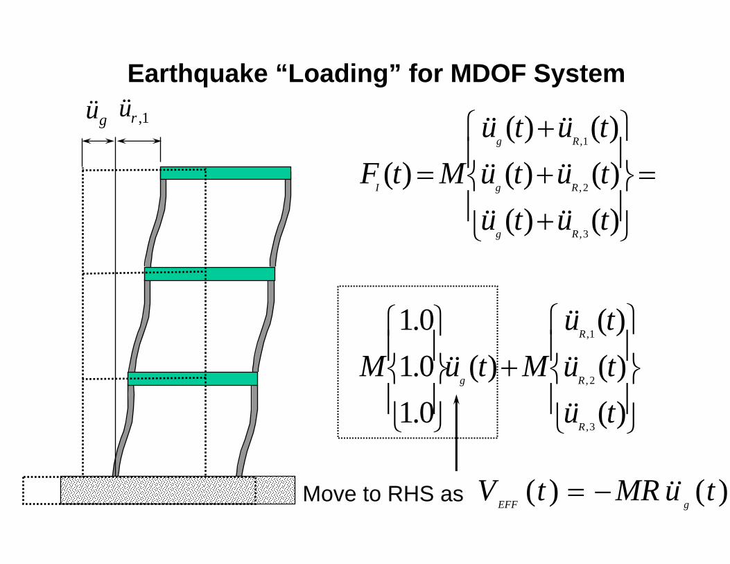
+++
=
)()()(
)(0.10.10.1
)()()()()()(
)(
3,
2,
1,
3,
2,
1,
tututu
MtuM
tutututututu
MtF
R
R
R
g
Rg
Rg
Rg
I
Move to RHS as )()( tuMRtVgEFF
−=
Earthquake “Loading” for MDOF System
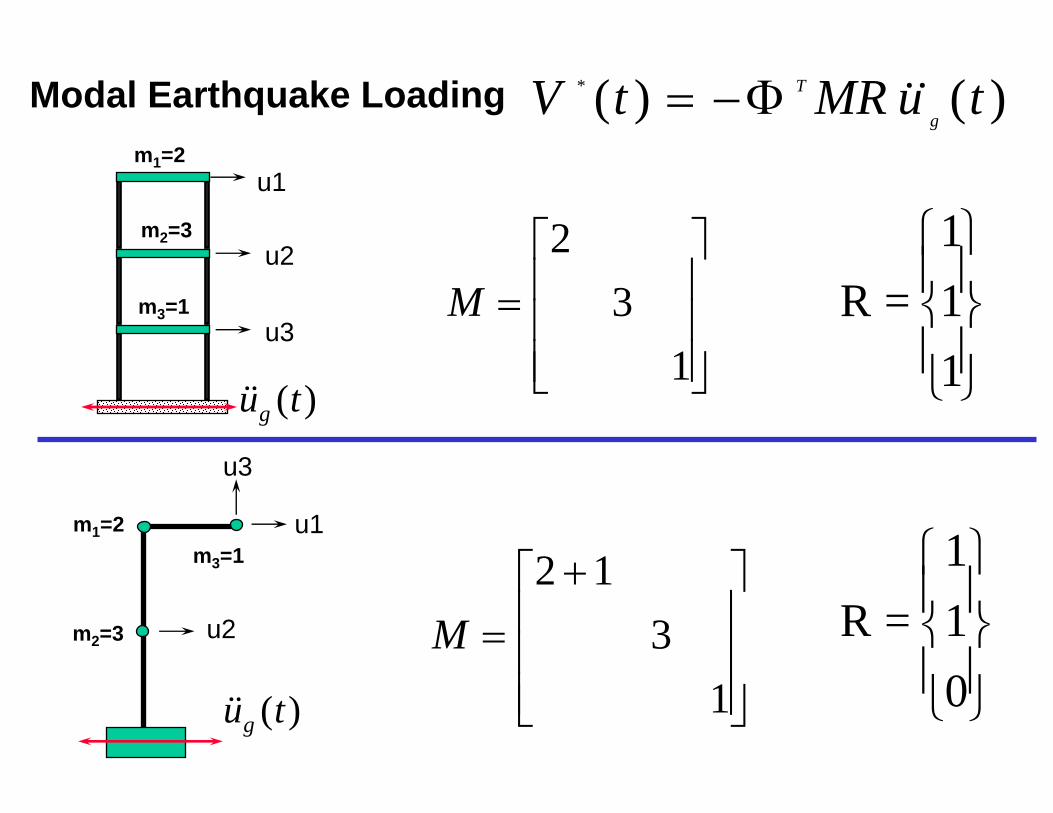
)()(* tuMRtVg
TΦ−=
⎪⎭
⎪⎬
⎫
⎪⎩
⎪⎨
⎧
111
=R
m1=2
m2=3
m3=1u1
u2
u3
M =+⎡
⎣
⎢⎢⎢
⎤
⎦
⎥⎥⎥
2 13
1 ⎪⎭
⎪⎬
⎫
⎪⎩
⎪⎨
⎧
011
=R
u1
u2
u3
m1=2
m2=3
m3=1 M =⎡
⎣
⎢⎢⎢
⎤
⎦
⎥⎥⎥
23
1
Modal Earthquake Loading
( )u tg
( )u tg
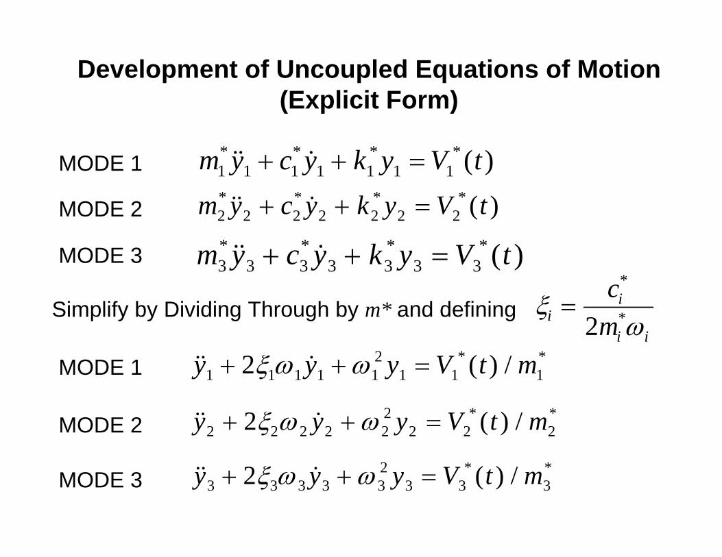
m y c y k y V t1 1 1 1 1 1 1* * * * ( )+ + =
m y c y k y V t3 3 3 3 3 3 3* * * * ( )+ + =
m y c y k y V t2 2 2 2 2 2 2* * * * ( )+ + =
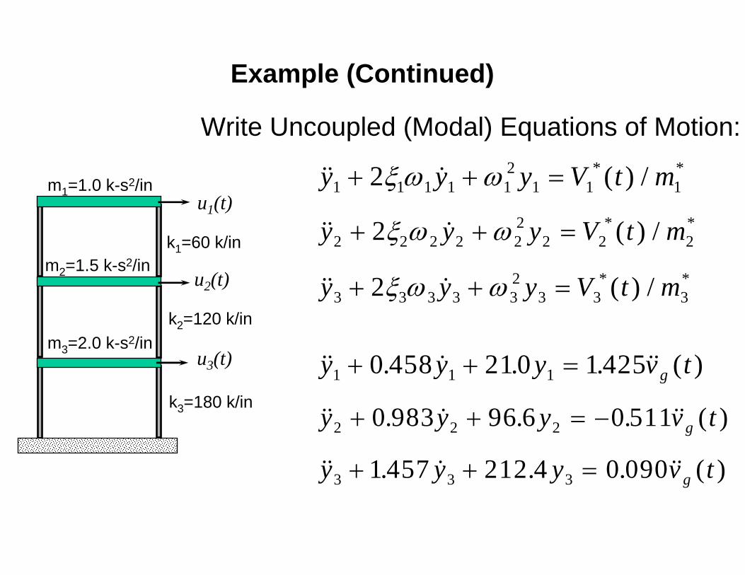
( ) /* *y y y V t m1 1 1 1 12
1 1 12+ + =ξ ω ω
( ) /* *y y y V t m2 2 2 2 22
2 2 22+ + =ξ ω ω
( ) /* *y y y V t m3 3 3 3 32
3 3 32+ + =ξ ω ω
Simplify by Dividing Through by m* and defining ξωi
i
i i
cm
=*
*2
Development of Uncoupled Equations of Motion(Explicit Form)
MODE 1
MODE 2
MODE 3
MODE 1
MODE 2
MODE 3
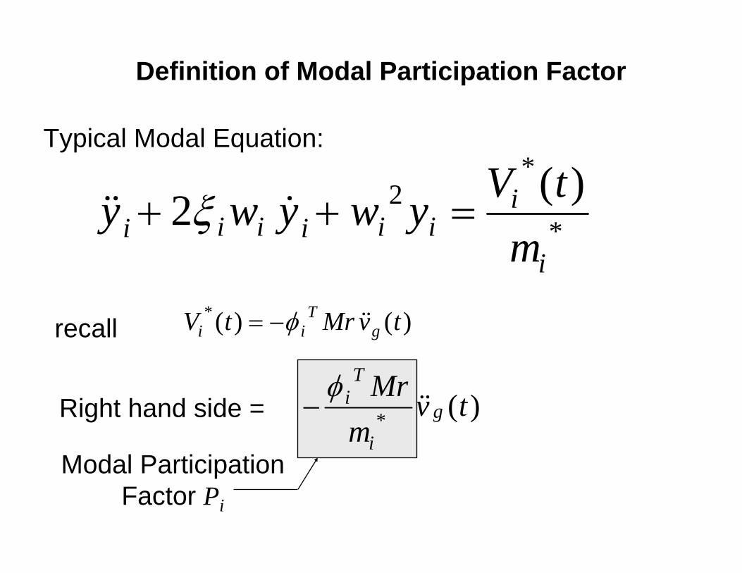
Definition of Modal Participation Factor
Typical Modal Equation:
( )*
*y w y w y V tmi i i i i ii
i
+ + =2 2ξ
recall V t Mr v ti iT
g*( ) ( )= −φ
Right hand side = −φ i
T
ig
Mrm
v t* ( )
Modal Participation Factor Pi
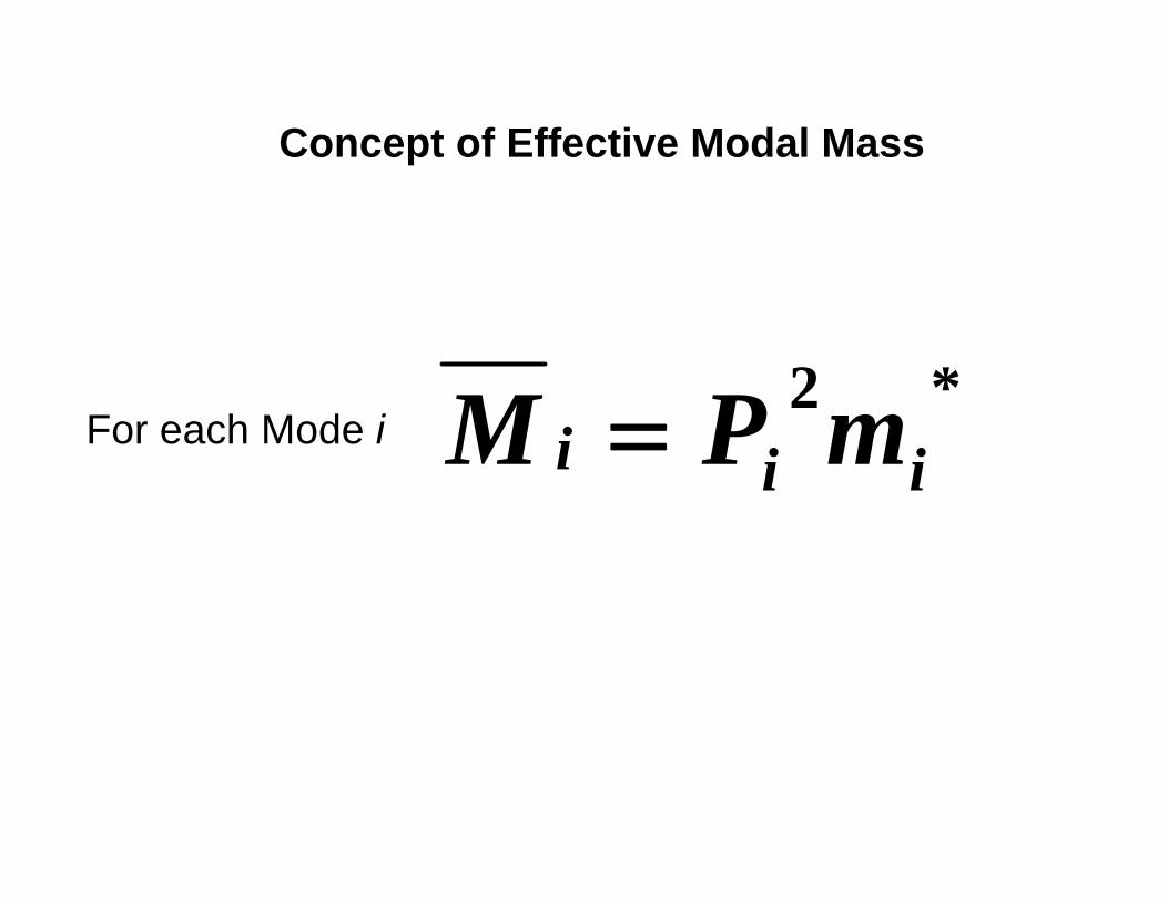
Concept of Effective Modal Mass
For each Mode i M P mi i i= 2 *
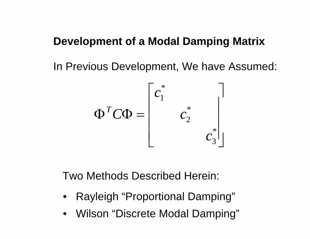
In Previous Development, We have Assumed:
Φ ΦTCc
cc
=
⎡
⎣
⎢⎢⎢
⎤
⎦
⎥⎥⎥
1
2
3
*
*
*
• Rayleigh “Proportional Damping”• Wilson “Discrete Modal Damping”
Development of a Modal Damping Matrix
Two Methods Described Herein:

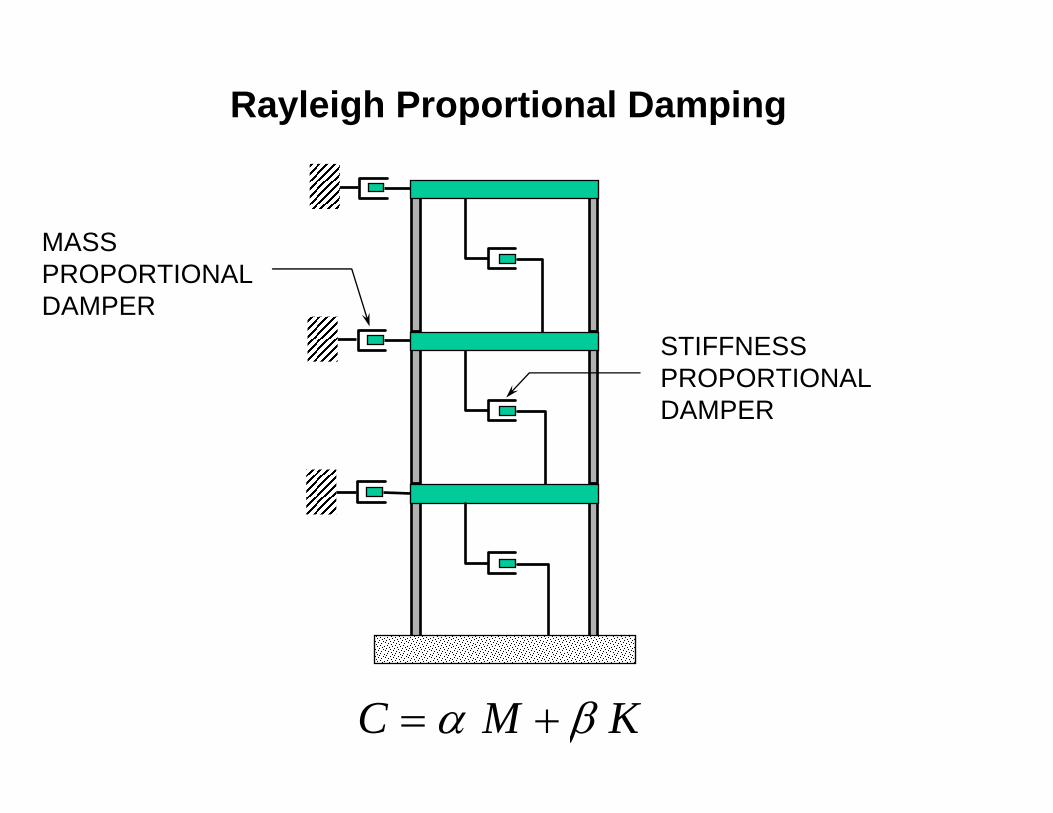
MASSPROPORTIONALDAMPER
STIFFNESSPROPORTIONALDAMPER
C M K= +α β
Rayleigh Proportional Damping
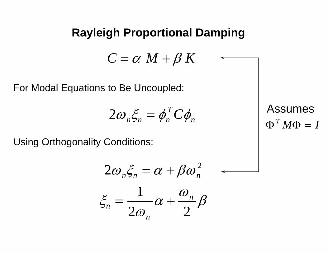
C M K= +α β
For Modal Equations to Be Uncoupled:
2ω ξ φ φn n nT
nC=
Using Orthogonality Conditions:
2 2ω ξ α βωn n n= +
ξω
α ω βnn
n= +1
2 2
Rayleigh Proportional Damping
Φ ΦT M I=Assumes
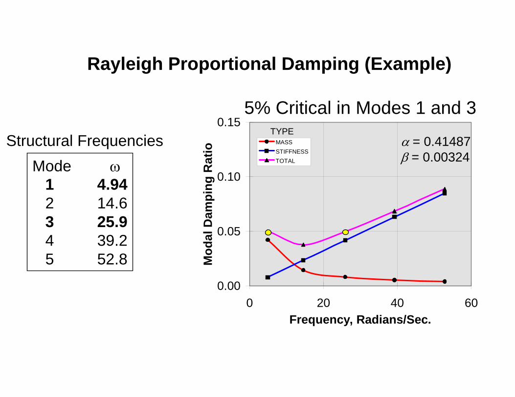
Mode ω1 4.942 14.63 25.94 39.25 52.8
Structural Frequencies
Rayleigh Proportional Damping (Example)
0.00
0.05
0.10
0.15
0 20 40 60Frequency, Radians/Sec.
Mod
al D
ampi
ng R
atio
MASSSTIFFNESSTOTAL
TYPEα = 0.41487β = 0.00324
5% Critical in Modes 1 and 3
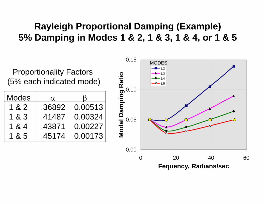
Modes α β1 & 2 .36892 0.005131 & 3 .41487 0.003241 & 4 .43871 0.002271 & 5 .45174 0.00173
Proportionality Factors (5% each indicated mode)
Rayleigh Proportional Damping (Example)5% Damping in Modes 1 & 2, 1 & 3, 1 & 4, or 1 & 5
0.00
0.05
0.10
0.15
0 20 40 60Fequency, Radians/sec
Mod
al D
ampi
ng R
atio
1,21,31,41,5
MODES
MASSPROPORTIONALDAMPER
STIFFNESSPROPORTIONALDAMPER
C M K= +α β
Rayleigh Proportional Damping
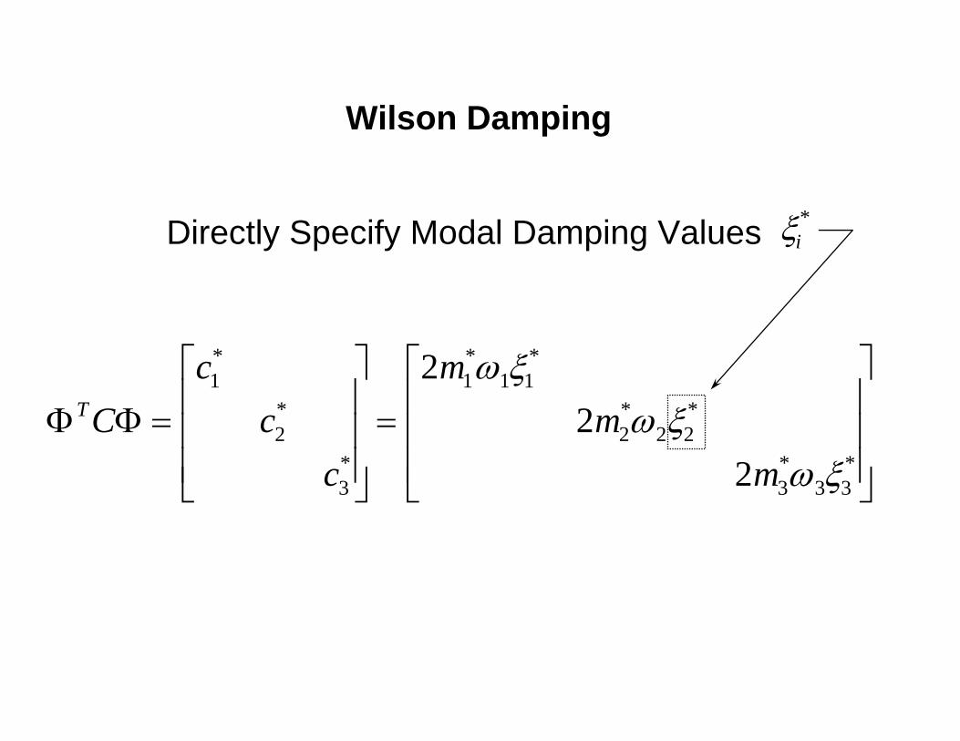
Wilson Damping
Directly Specify Modal Damping Values ξi*
Φ ΦTCc
cc
mm
m=
⎡
⎣
⎢⎢⎢
⎤
⎦
⎥⎥⎥=
⎡
⎣
⎢⎢⎢
⎤
⎦
⎥⎥⎥
1
2
3
1 1 1
2 2 2
3 3 3
22
2
*
*
*
* *
* *
* *
ω ξω ξ
ω ξ
Φ ΦT
n n
n n
C c= •••
L
N
MMMMMM
O
Q
PPPPPP
=
− −
22
22
1 1
2 2
1 1
ξ ωξ ω
ξ ωξ ω
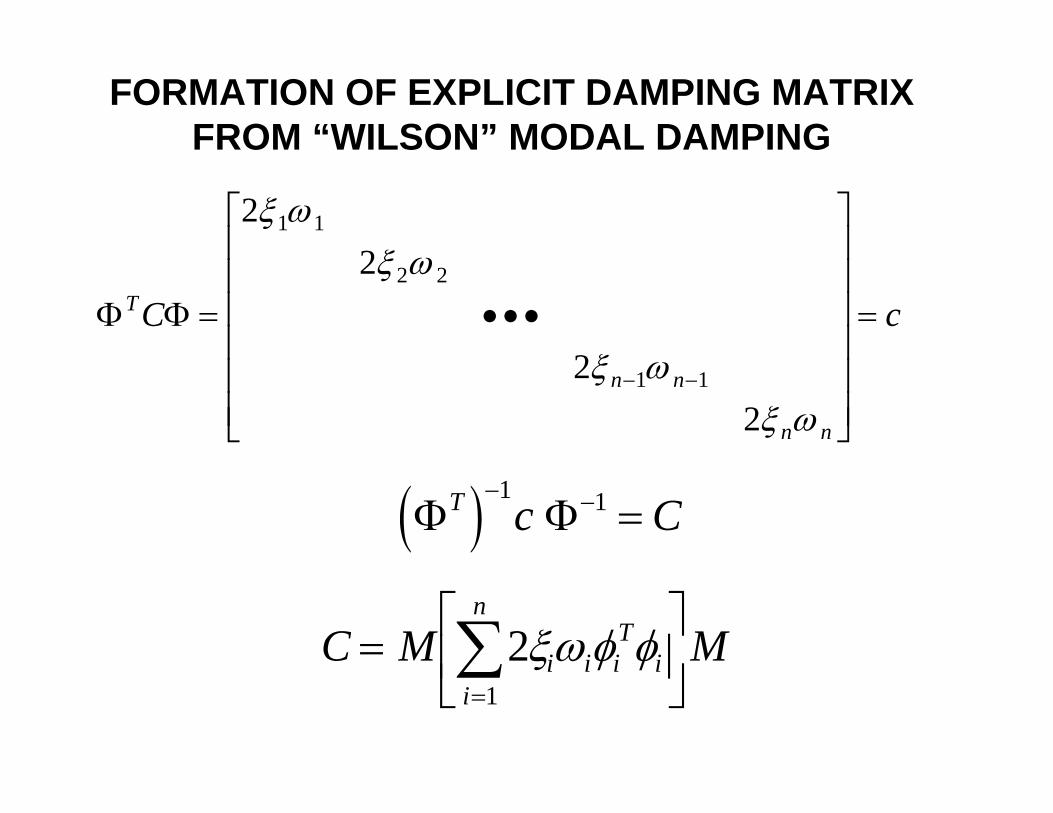
( )Φ ΦT c C− − =
1 1
C M Mi i iT
ii
n
=⎡
⎣⎢
⎤
⎦⎥
=∑2
1
ξω φ φ
FORMATION OF EXPLICIT DAMPING MATRIXFROM “WILSON” MODAL DAMPING
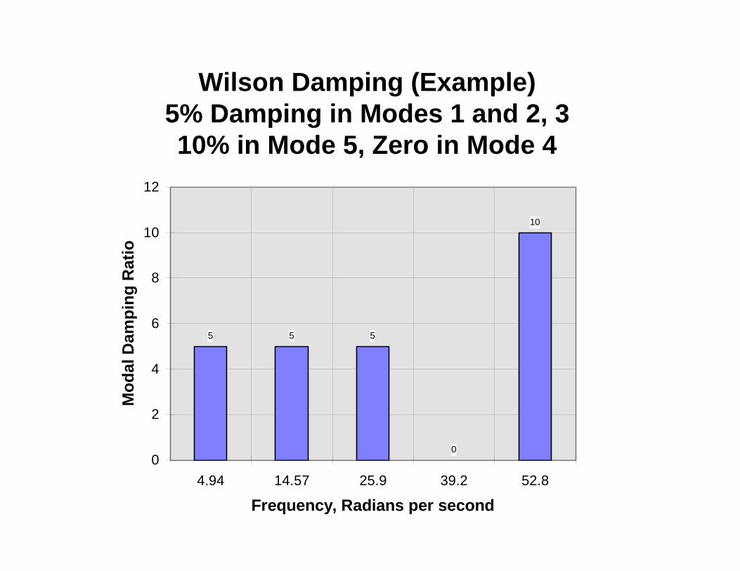
5 5 5
0
10
0
2
4
6
8
10
12
4.94 14.57 25.9 39.2 52.8
Frequency, Radians per second
Mod
al D
ampi
ng R
atio
Wilson Damping (Example)5% Damping in Modes 1 and 2, 310% in Mode 5, Zero in Mode 4
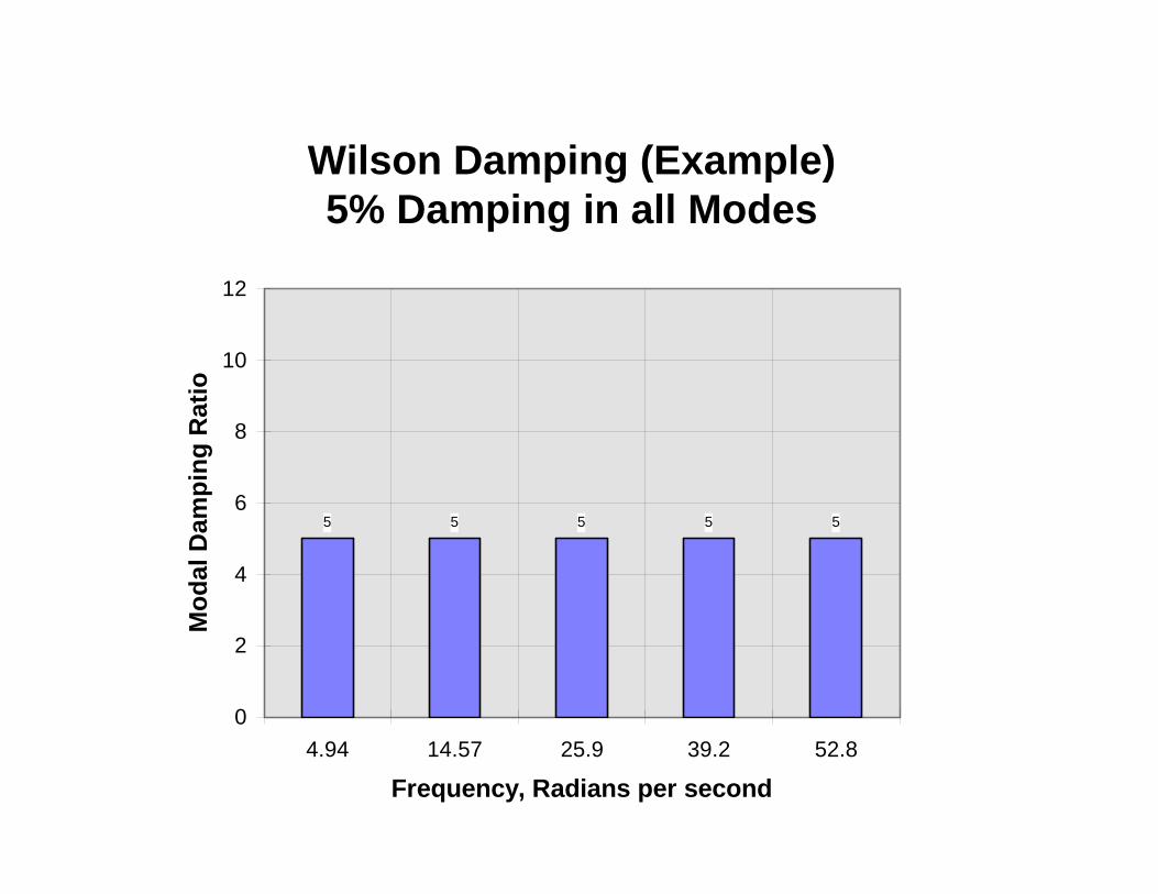
Wilson Damping (Example)5% Damping in all Modes
5 5 5 5 5
0
2
4
6
8
10
12
4.94 14.57 25.9 39.2 52.8
Frequency, Radians per second
Mod
al D
ampi
ng R
atio
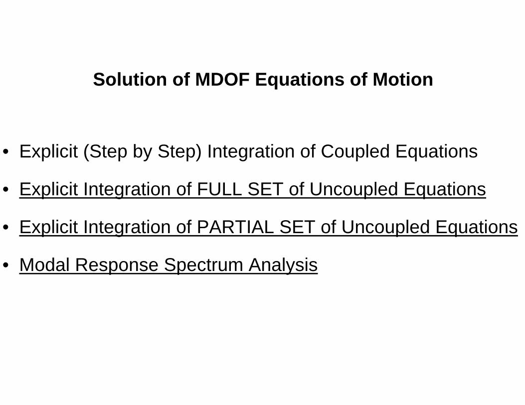
Solution of MDOF Equations of Motion
• Explicit (Step by Step) Integration of Coupled Equations
• Explicit Integration of FULL SET of Uncoupled Equations
• Explicit Integration of PARTIAL SET of Uncoupled Equations
• Modal Response Spectrum Analysis
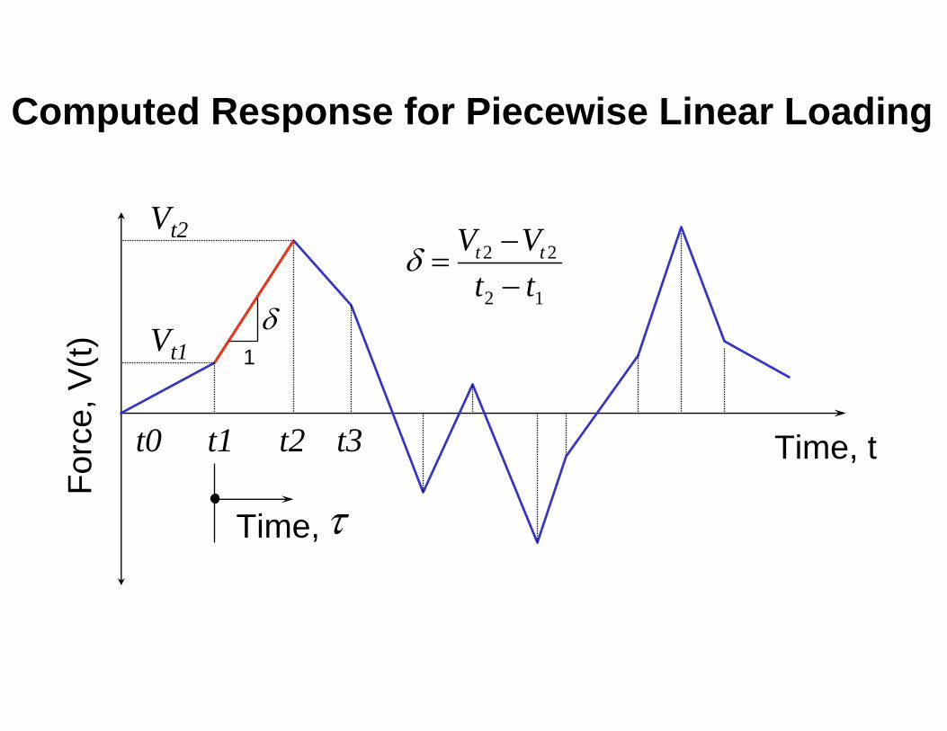
Time, t
Forc
e, V
(t)
t1 t3t2t0
Vt2
Vt1 1δ
Time, τ
δ =−−
V Vt tt t2 2
2 1
Computed Response for Piecewise Linear Loading
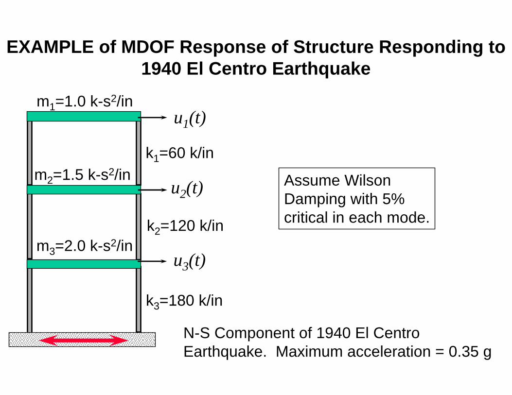
EXAMPLE of MDOF Response of Structure Responding to1940 El Centro Earthquake
k3=180 k/in
u1(t)
u2(t)
u3(t)
k1=60 k/in
k2=120 k/in
m1=1.0 k-s2/in
m2=1.5 k-s2/in
m3=2.0 k-s2/in
Assume WilsonDamping with 5%critical in each mode.
N-S Component of 1940 El CentroEarthquake. Maximum acceleration = 0.35 g
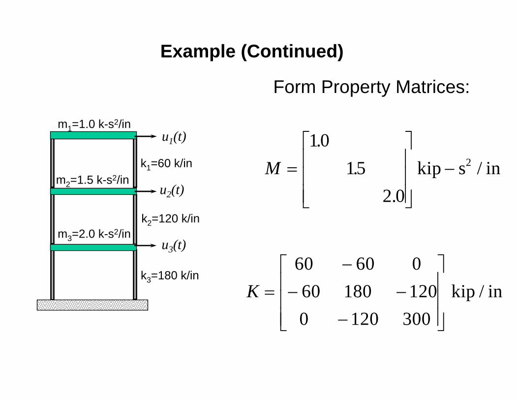
M =⎡
⎣
⎢⎢⎢
⎤
⎦
⎥⎥⎥
−10
152 0
..
.kip s / in2
k3=180 k/in
u1(t)
u2(t)
u3(t)
k1=60 k/in
k2=120 k/in
m1=1.0 k-s2/in
m2=1.5 k-s2/in
m3=2.0 k-s2/in
K =−
− −−
⎡
⎣
⎢⎢⎢
⎤
⎦
⎥⎥⎥
60 60 060 180 1200 120 300
kip / in
Form Property Matrices:
Example (Continued)
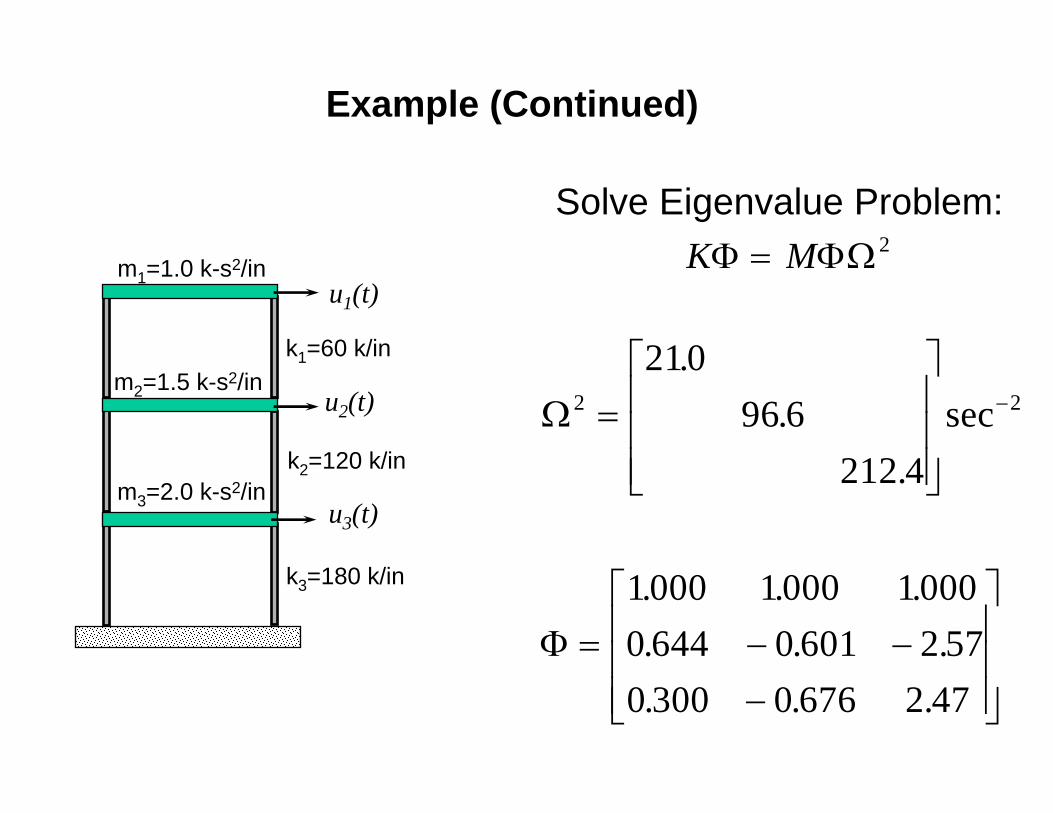
Ω2 2
21096 6
212 4=⎡
⎣
⎢⎢⎢
⎤
⎦
⎥⎥⎥
−
..
.sec
k3=180 k/in
u1(t)
u2(t)
u3(t)
k1=60 k/in
k2=120 k/in
m1=1.0 k-s2/in
m2=1.5 k-s2/in
m3=2.0 k-s2/in
Φ = − −−
⎡
⎣
⎢⎢⎢
⎤
⎦
⎥⎥⎥
1000 1000 10000 644 0 601 2 570 300 0 676 2 47
. . .
. . .
. . .
K MΦ ΦΩ= 2
Solve Eigenvalue Problem:
Example (Continued)
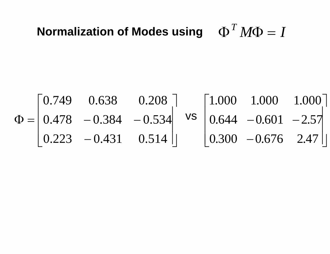
Normalization of Modes using Φ ΦT M I=
vs
⎥⎥⎥
⎦
⎤
⎢⎢⎢
⎣
⎡
−−−=Φ
514.0431.0223.0534.0384.0478.0
208.0638.0749.0
⎥⎥⎥
⎦
⎤
⎢⎢⎢
⎣
⎡
−−−
47.2676.0300.057.2601.0644.0
000.1000.1000.1
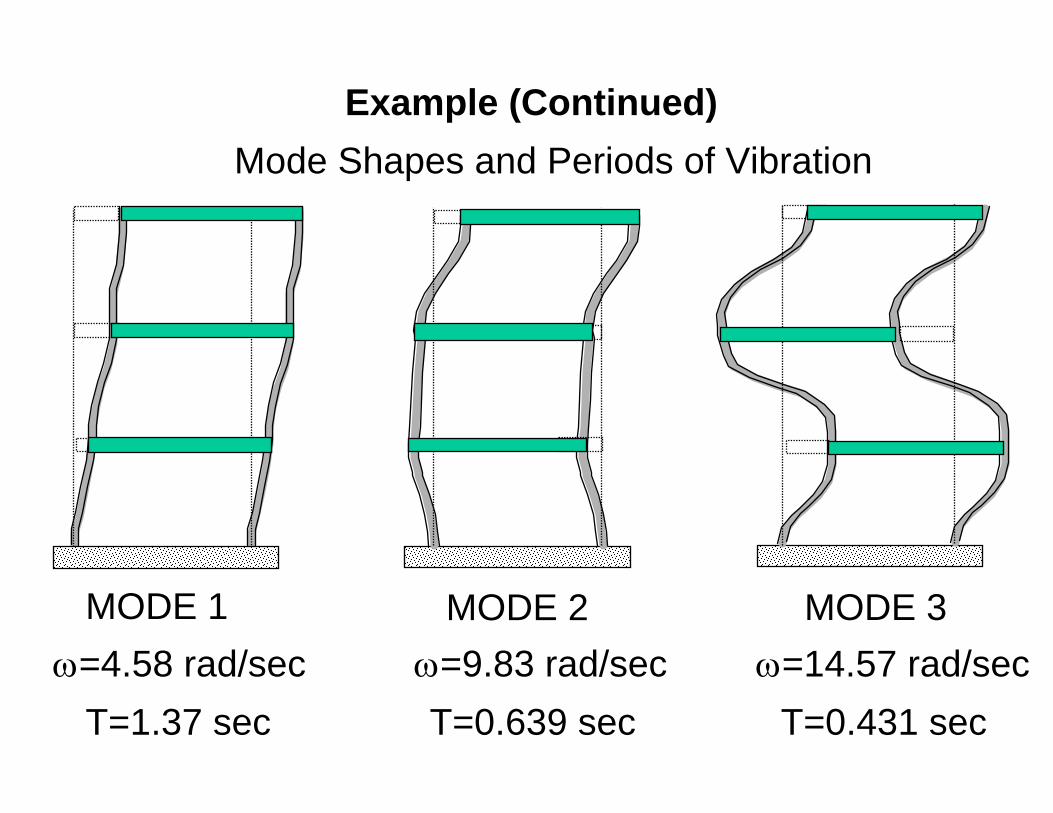
MODE 1 MODE 2 MODE 3
T=1.37 sec T=0.639 sec T=0.431 sec
Example (Continued)Mode Shapes and Periods of Vibration
ω=4.58 rad/sec ω=9.83 rad/sec ω=14.57 rad/sec
k3=180 k/in
u1(t)
u2(t)
u3(t)
k1=60 k/in
k2=120 k/in
m1=1.0 k-s2/in
m2=1.5 k-s2/in
m3=2.0 k-s2/in
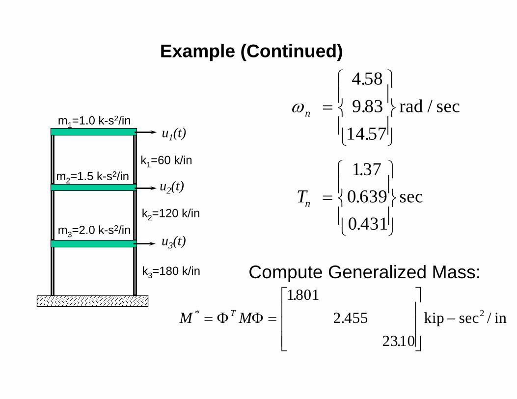
M MT*
..
.sec /= =
⎡
⎣
⎢⎢⎢
⎤
⎦
⎥⎥⎥
−Φ Φ1801
2 4552310
2kip in
ωn =⎧
⎨⎪
⎩⎪
⎫
⎬⎪
⎭⎪
4 589 83
14 57
.
..
/ secrad
Tn =⎧
⎨⎪
⎩⎪
⎫
⎬⎪
⎭⎪
1370 6390 431
...
sec
Compute Generalized Mass:
Example (Continued)
k3=180 k/in
u1(t)
u2(t)
u3(t)
k1=60 k/in
k2=120 k/in
m1=1.0 k-s2/in
m2=1.5 k-s2/in
m3=2.0 k-s2/in
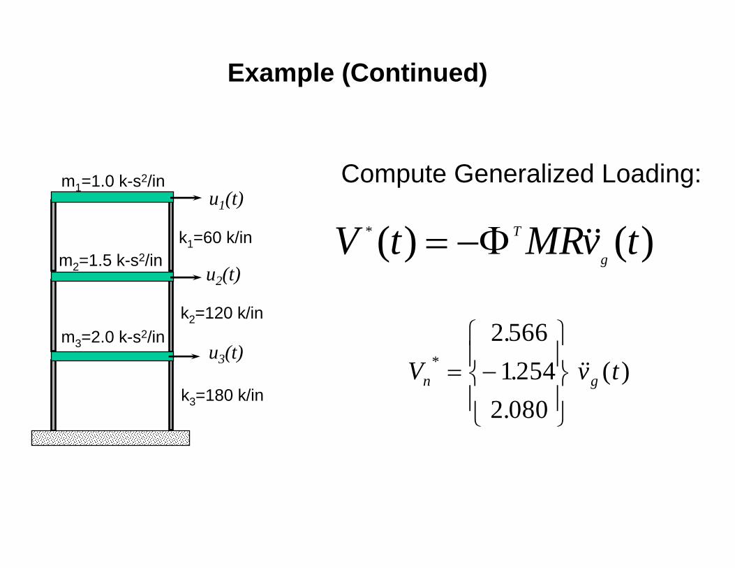
Compute Generalized Loading:
)()(* tvMRtVg
TΦ−=
V v tn g*
..
.( )= −
⎧
⎨⎪
⎩⎪
⎫
⎬⎪
⎭⎪
2 5661254
2 080
Example (Continued)
( ) /* *y y y V t m1 1 1 1 12
1 1 12+ + =ξ ω ω
( ) /* *y y y V t m2 2 2 2 22
2 2 22+ + =ξ ω ω
( ) /* *y y y V t m3 3 3 3 32
3 3 32+ + =ξ ω ω
k3=180 k/in
u1(t)
u2(t)
u3(t)
k1=60 k/in
k2=120 k/in
m1=1.0 k-s2/in
m2=1.5 k-s2/in
m3=2.0 k-s2/in. . . ( )y y y v tg1 1 10 458 21 0 1 425+ + =
. . . ( )y y y v tg2 2 20 983 96 6 0 511+ + = −
. . . ( )y y y v tg3 3 31 457 212 4 0 090+ + =
Write Uncoupled (Modal) Equations of Motion:
Example (Continued)
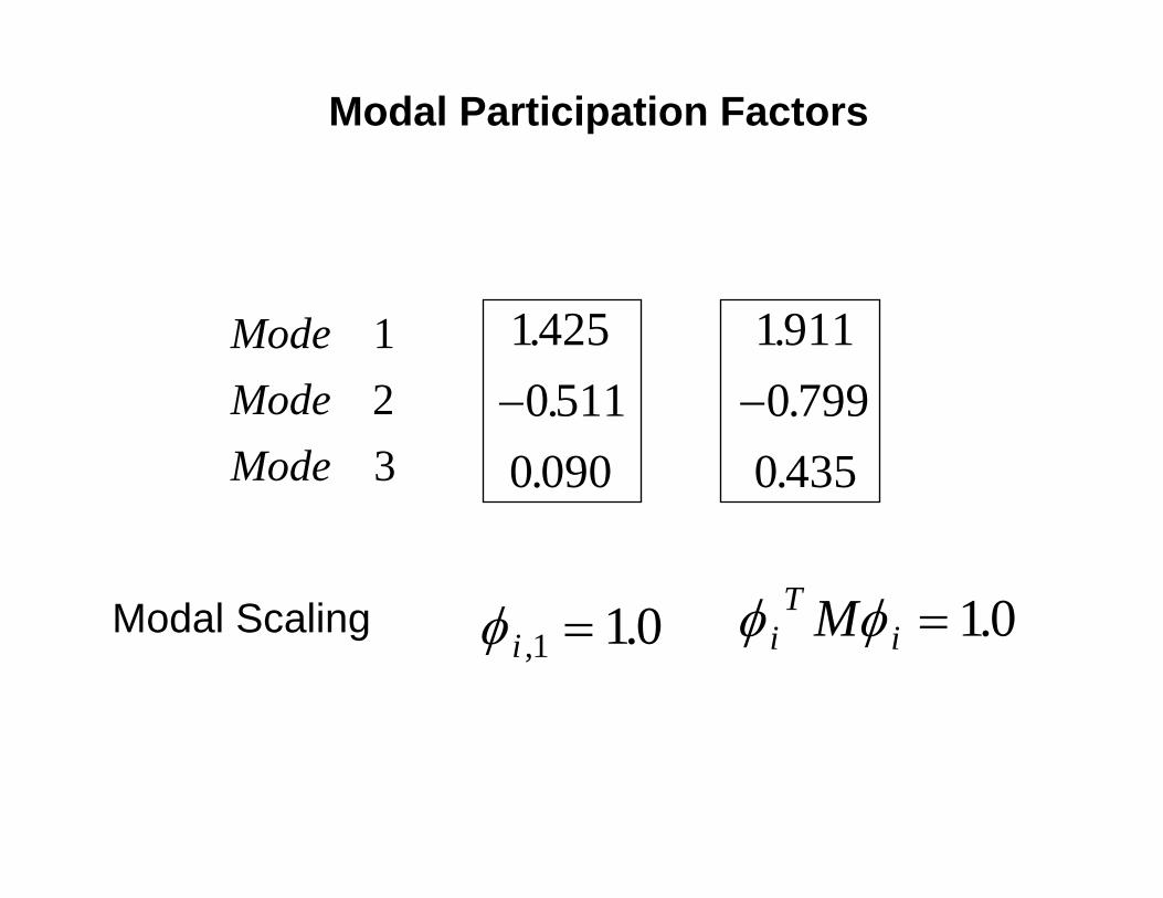
Modal Participation Factors
14250 511
0 090
..
.−
19110 799
0 435
..
.−
ModeModeMode
123
Modal Scaling φ i , .1 10= φ φiT
iM = 10.
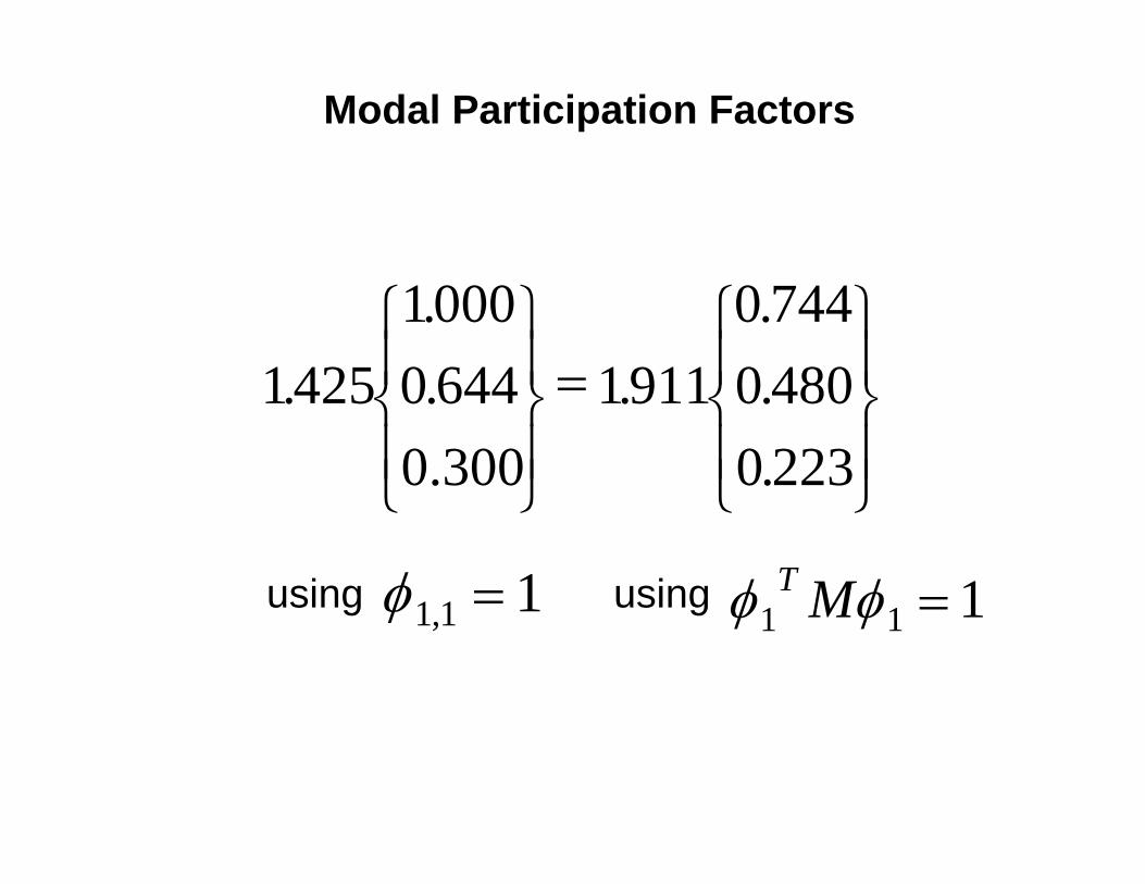
Modal Participation Factors
142510000 644 1911
0 7440 4800 223
... .
.
.
.
RS|T|
UV|W|=RS|T|
UV|W|
using usingφ1 1 1, = φ φ1 1 1T M =
0.300
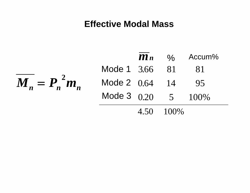
Effective Modal Mass
M P mn n n= 2Mode 1Mode 2Mode 3
3 66 81 810 64 14 950 20 5 100%
.
.
.
Accum%
4.50 100%
%mn
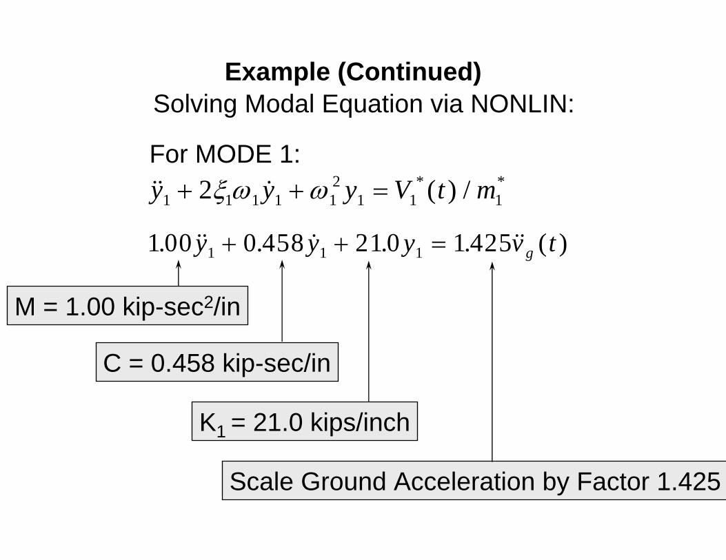
( ) /* *y y y V t m1 1 1 1 12
1 1 12+ + =ξ ω ω
1 00 0 458 21 0 1 4251 1 1. . . . ( )y y y v tg+ + =
M = 1.00 kip-sec2/in
C = 0.458 kip-sec/in
K1 = 21.0 kips/inch
Scale Ground Acceleration by Factor 1.425
Example (Continued)Solving Modal Equation via NONLIN:
For MODE 1:
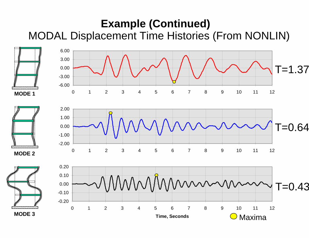
MODE 1
Example (Continued)
MODE 2
MODE 3
-2.00
-1.00
0.00
1.00
2.00
0 1 2 3 4 5 6 7 8 9 10 11 12
MODAL Displacement Time Histories (From NONLIN)
-6.00
-3.00
0.00
3.00
6.00
0 1 2 3 4 5 6 7 8 9 10 11 12
-0.20
-0.10
0.00
0.10
0.20
0 1 2 3 4 5 6 7 8 9 10 11 12
Time, Seconds
T=1.37
T=0.64
T=0.43
Maxima
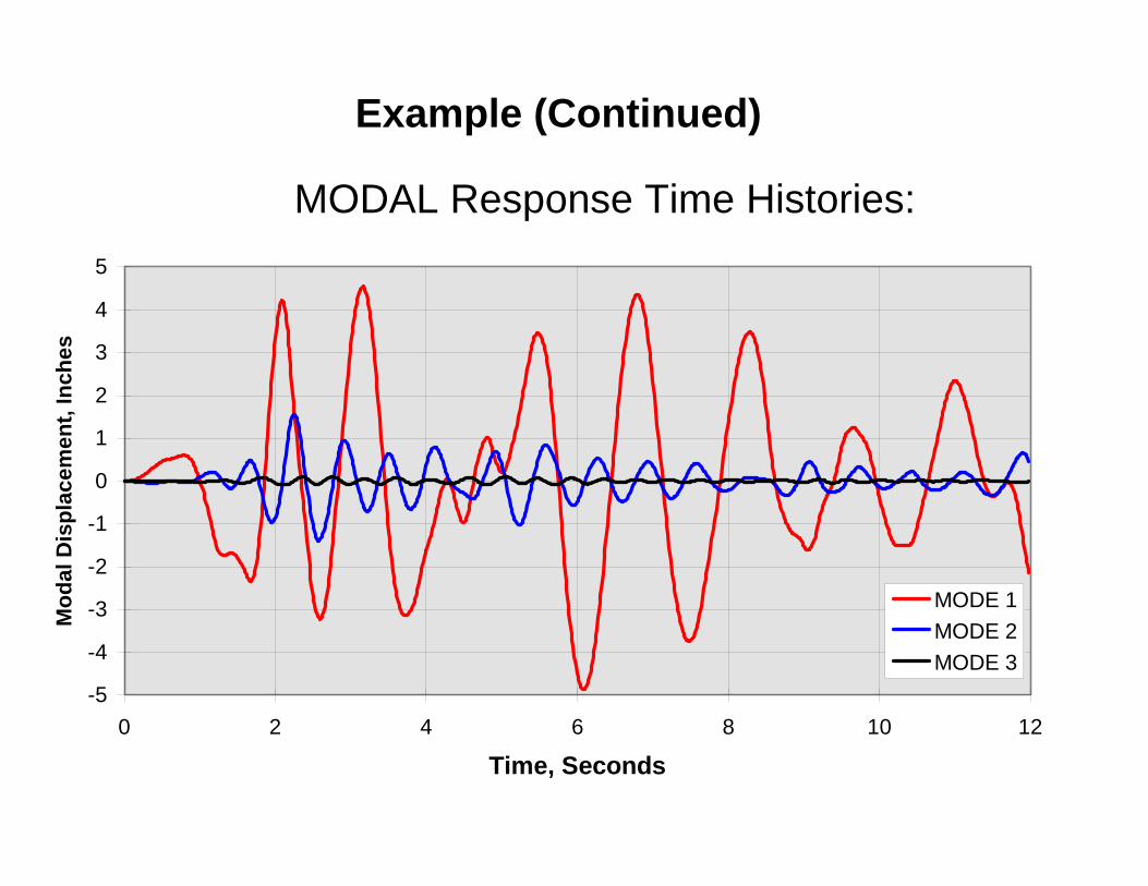
-5
-4
-3
-2
-1
0
1
2
3
4
5
0 2 4 6 8 10 12
Time, Seconds
Mod
al D
ispl
acem
ent,
Inch
es
MODE 1MODE 2MODE 3
MODAL Response Time Histories:
Example (Continued)
-6-4-20246
0 1 2 3 4 5 6 7 8 9 10 11 12
-6-4-20246
0 1 2 3 4 5 6 7 8 9 10 11 12
Time, Seconds
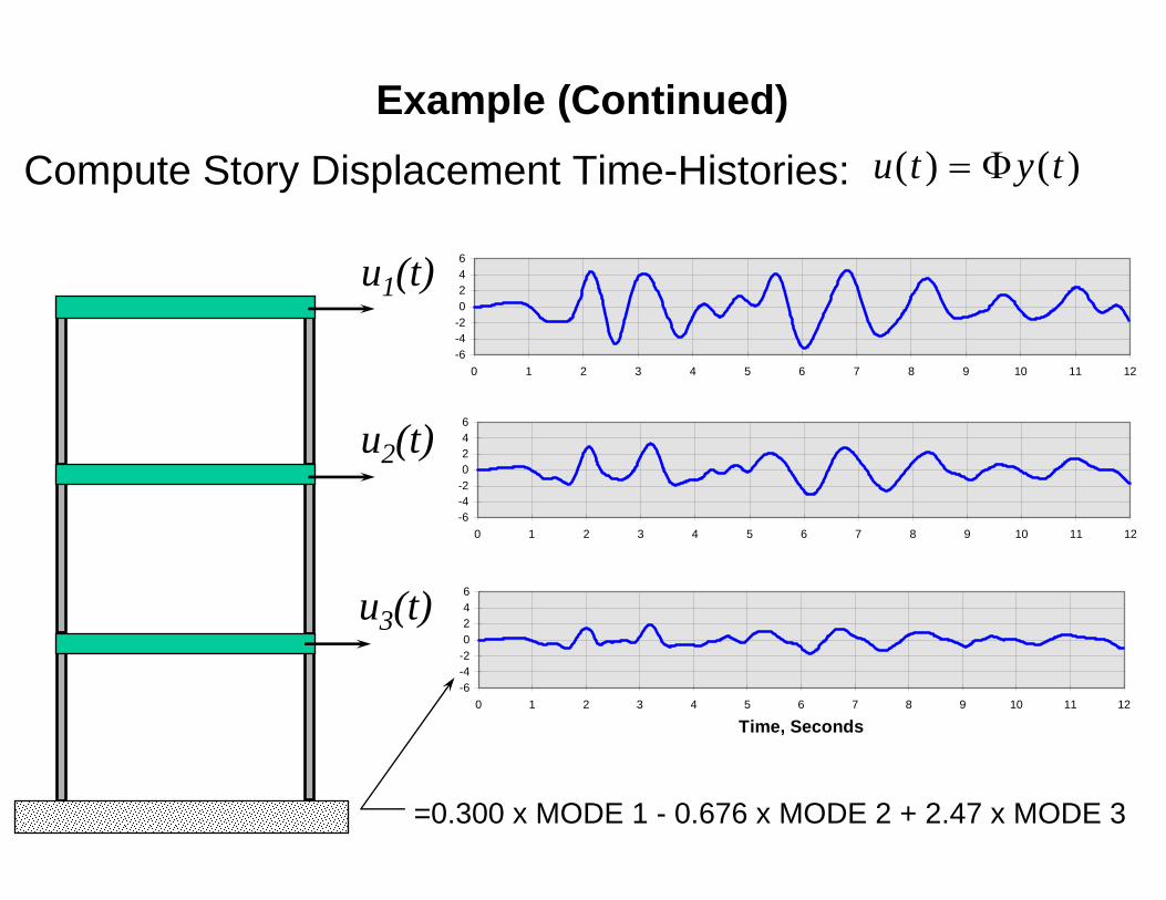
u1(t)
u2(t)
u3(t)
=0.300 x MODE 1 - 0.676 x MODE 2 + 2.47 x MODE 3
Example (Continued)Compute Story Displacement Time-Histories:
-6-4-20246
0 1 2 3 4 5 6 7 8 9 10 11 12
u t y t( ) ( )= Φ
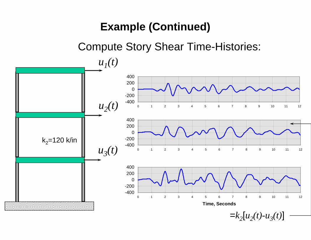
=k2[u2(t)-u3(t)]
Example (Continued)
Compute Story Shear Time-Histories:
-400-200
0200400
0 1 2 3 4 5 6 7 8 9 10 11 12
-400-200
0200400
0 1 2 3 4 5 6 7 8 9 10 11 12
-400-200
0200400
0 1 2 3 4 5 6 7 8 9 10 11 12
Time, Seconds
u2(t)
u3(t)k2=120 k/in
u1(t)
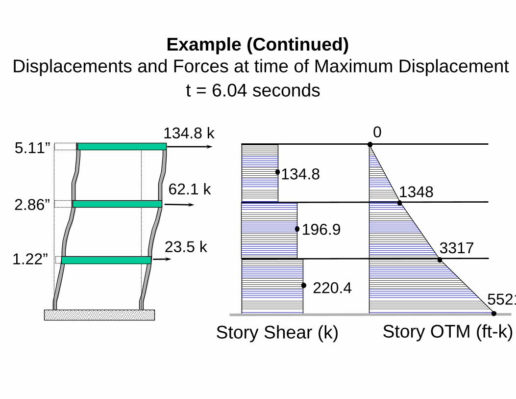
134.8 k
62.1 k
23.5 k
5.11”
2.86”
1.22”
134.8
196.9
220.4
1348
3317
5521
0
Displacements and Forces at time of Maximum Displacementt = 6.04 seconds
Story Shear (k) Story OTM (ft-k)
Example (Continued)
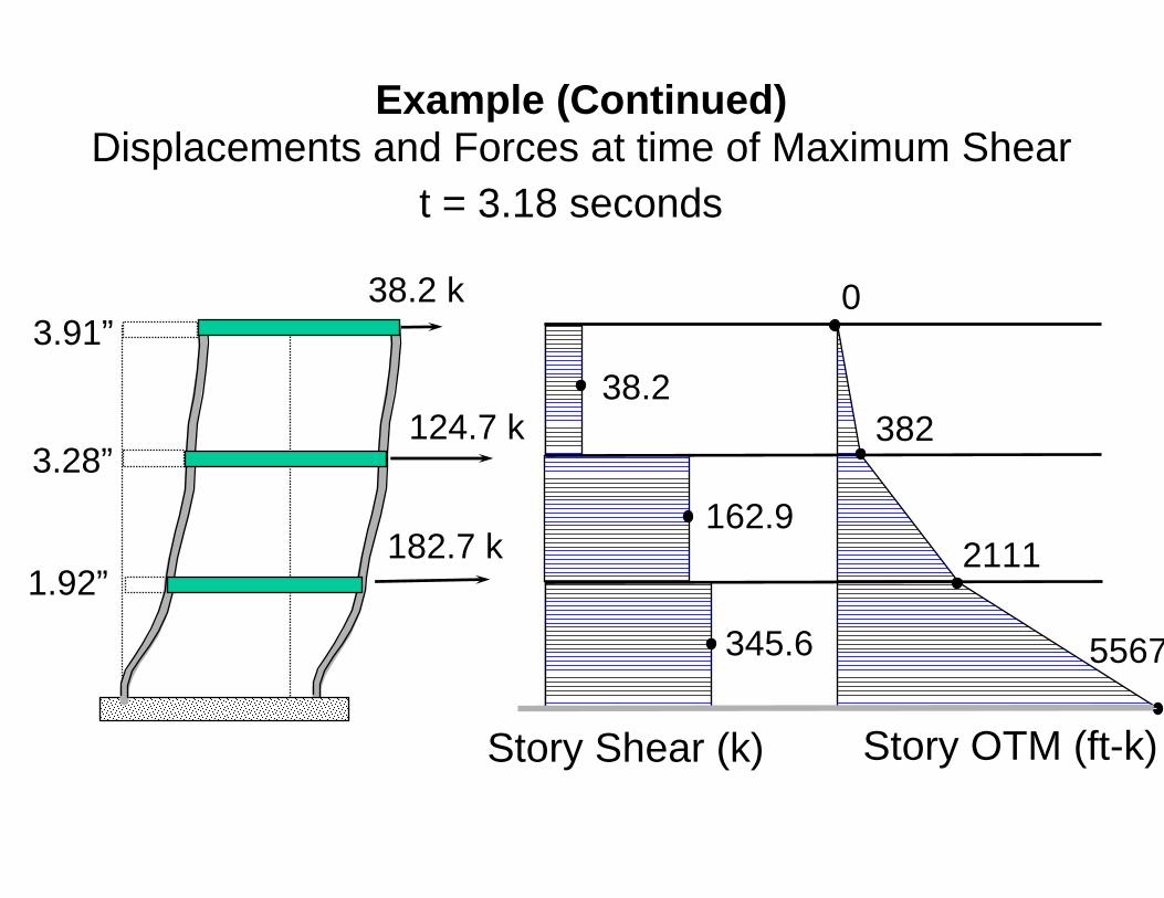
38.2 k
182.7 k
124.7 k
3.91”
3.28”
1.92”
38.2
162.9
345.6
382
2111
5567
0
Displacements and Forces at time of Maximum Sheart = 3.18 seconds
Story Shear (k) Story OTM (ft-k)
Example (Continued)
0.00
1.00
2.00
3.00
4.00
5.00
6.00
7.00
0.00 0.20 0.40 0.60 0.80 1.00 1.20 1.40 1.60 1.80 2.00
Period, Seconds
Spec
tral
Dis
plac
emen
t, In
ches
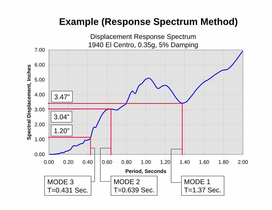
1.20”
3.04”
3.47”
MODE 3T=0.431 Sec.
MODE 2T=0.639 Sec.
MODE 1T=1.37 Sec.
Displacement Response Spectrum1940 El Centro, 0.35g, 5% Damping
Example (Response Spectrum Method)
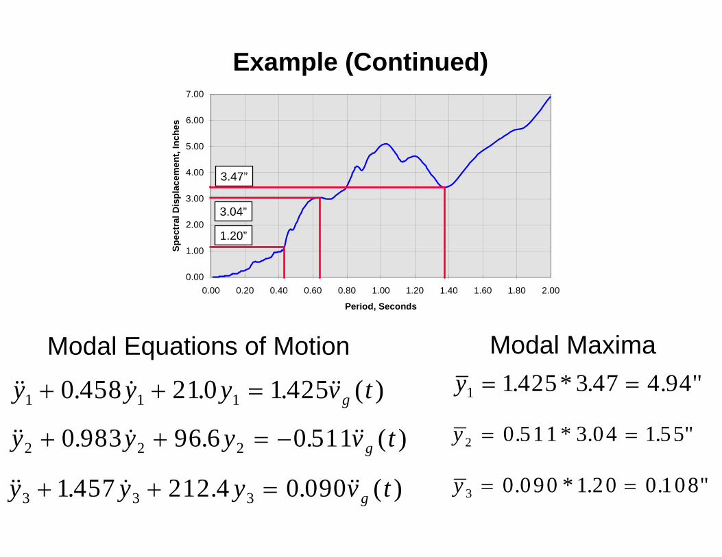
. . . ( )y y y v tg1 1 10 458 21 0 1 425+ + =
. . . ( )y y y v tg2 2 20 983 96 6 0 511+ + = −
. . . ( )y y y v tg3 3 31 457 212 4 0 090+ + =
0.00
1.00
2.00
3.00
4.00
5.00
6.00
7.00
0.00 0.20 0.40 0.60 0.80 1.00 1.20 1.40 1.60 1.80 2.00
Period, Seconds
Spec
tral
Dis
plac
emen
t, In
ches
1.20”
3.04”
3.47”
y1 1 425 3 47 4 94= =. * . . "
y 2 0 511 3 04 1 55= =. * . . "
y 3 0 090 1 20 0 108= =. * . . "
Modal Equations of Motion Modal Maxima
Example (Continued)
0.00
1.00
2.00
3.00
4.00
5.00
6.00
7.00
0.00 0.20 0.40 0.60 0.80 1.00 1.20 1.40 1.60 1.80 2.00
Period, Seconds
Spec
tral
Dis
plac
emen
t, In
ches
1.20 x 0.090”
3.04 x 0.511”
3.47x 1.425”
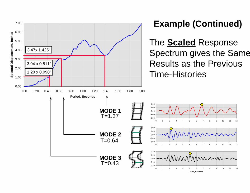
MODE 1
MODE 2
MODE 3
-2.00
-1.00
0.00
1.00
2.00
0 1 2 3 4 5 6 7 8 9 10 11 12
-6.00
-3.00
0.00
3.00
6.00
0 1 2 3 4 5 6 7 8 9 10 11 12
-0.20
-0.10
0.00
0.10
0.20
0 1 2 3 4 5 6 7 8 9 10 11 12
Time, Seconds
T=1.37
T=0.64
T=0.43
The Scaled ResponseSpectrum gives the SameResults as the PreviousTime-Histories
Example (Continued)
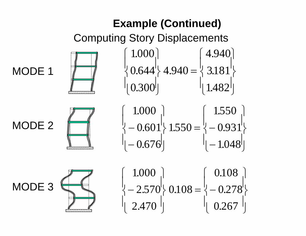
10000 6440 300
4 9404 94031811482
.
.
..
.
..
⎧
⎨⎪
⎩⎪
⎫
⎬⎪
⎭⎪
=⎧
⎨⎪
⎩⎪
⎫
⎬⎪
⎭⎪
10000 6010 676
155015500 9311048
...
....
−−
⎧
⎨⎪
⎩⎪
⎫
⎬⎪
⎭⎪
= −−
⎧
⎨⎪
⎩⎪
⎫
⎬⎪
⎭⎪
10002 570
2 4700108
01080 278
0 267
..
..
..
.−⎧
⎨⎪
⎩⎪
⎫
⎬⎪
⎭⎪
= −⎧
⎨⎪
⎩⎪
⎫
⎬⎪
⎭⎪
MODE 1
MODE 2
MODE 3
Example (Continued)Computing Story Displacements
4 940 1550 01083181 0 931 10481482 1048 0 267
518348184
2 2 2
2 2 2
2 2 2
. . .
. . .. . .
.
.
.
+ ++ ++ +
⎧
⎨⎪
⎩⎪
⎫
⎬⎪
⎭⎪=⎧
⎨⎪
⎩⎪
⎫
⎬⎪
⎭⎪
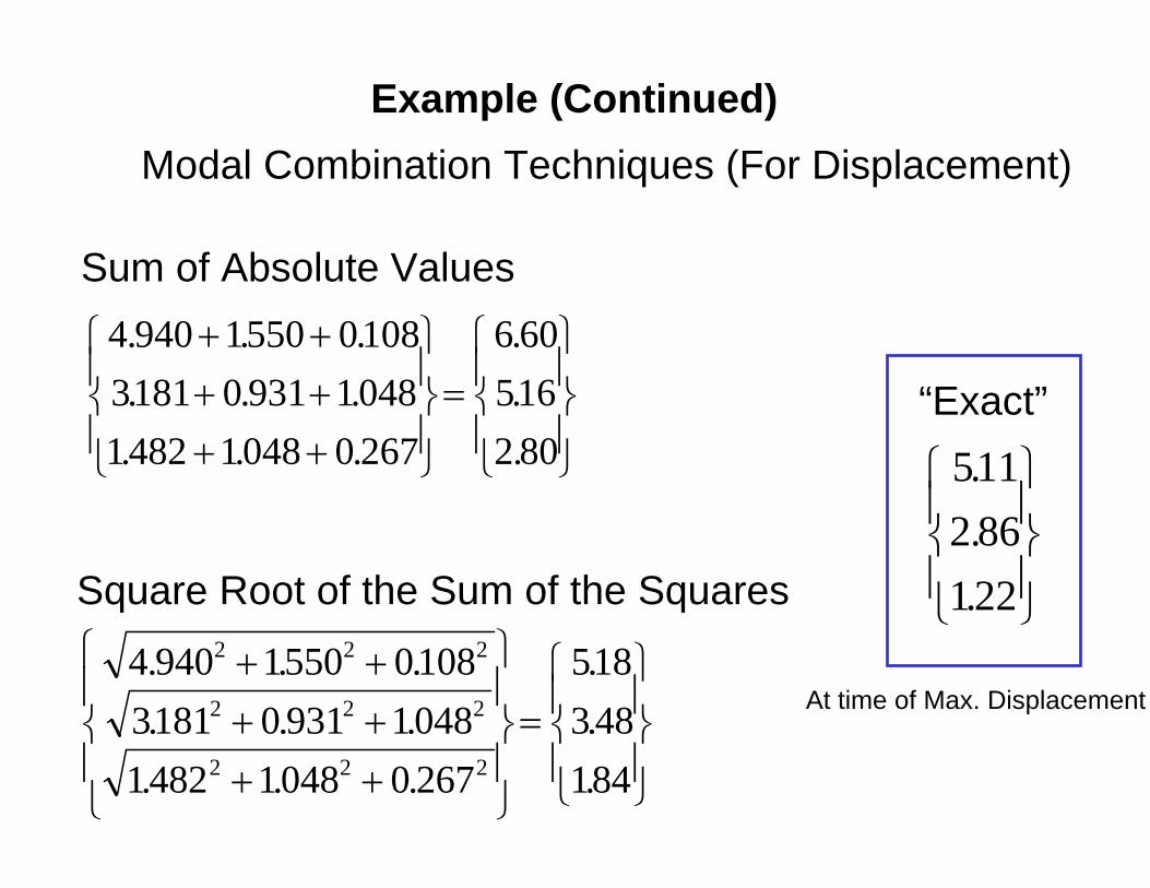
Square Root of the Sum of the Squares
4 940 1550 01083181 0 931 10481482 1048 0 267
6 605162 80
. . .
. . .. . .
.
.
.
+ ++ ++ +
⎧
⎨⎪
⎩⎪
⎫
⎬⎪
⎭⎪=⎧
⎨⎪
⎩⎪
⎫
⎬⎪
⎭⎪
Sum of Absolute Values
5112 86122
.
..
⎧
⎨⎪
⎩⎪
⎫
⎬⎪
⎭⎪
“Exact”
Example (Continued)Modal Combination Techniques (For Displacement)
At time of Max. Displacement
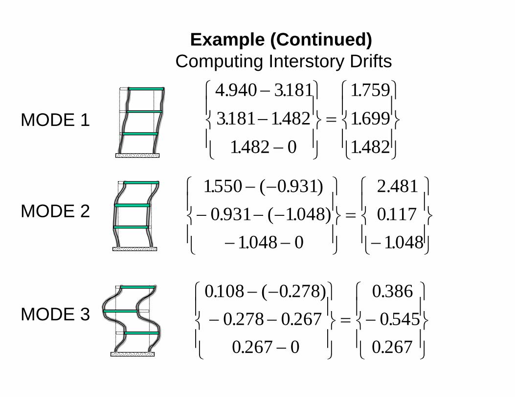
4 940 31813181 1482
1482 0
175916991482
. .
. ..
.
.
.
−−−
⎧
⎨⎪
⎩⎪
⎫
⎬⎪
⎭⎪=⎧
⎨⎪
⎩⎪
⎫
⎬⎪
⎭⎪
1550 0 9310 931 1048
1048 0
2 48101171048
. ( . ). ( . )
.
.
..
− −− − −
− −
⎧
⎨⎪
⎩⎪
⎫
⎬⎪
⎭⎪=
−
⎧
⎨⎪
⎩⎪
⎫
⎬⎪
⎭⎪
0108 0 2780 278 0 2670 267 0
0 3860 545
0 267
. ( . ). ..
..
.
− −− −
−
⎧
⎨⎪
⎩⎪
⎫
⎬⎪
⎭⎪= −⎧
⎨⎪
⎩⎪
⎫
⎬⎪
⎭⎪
MODE 1
MODE 2
MODE 3
Example (Continued)Computing Interstory Drifts
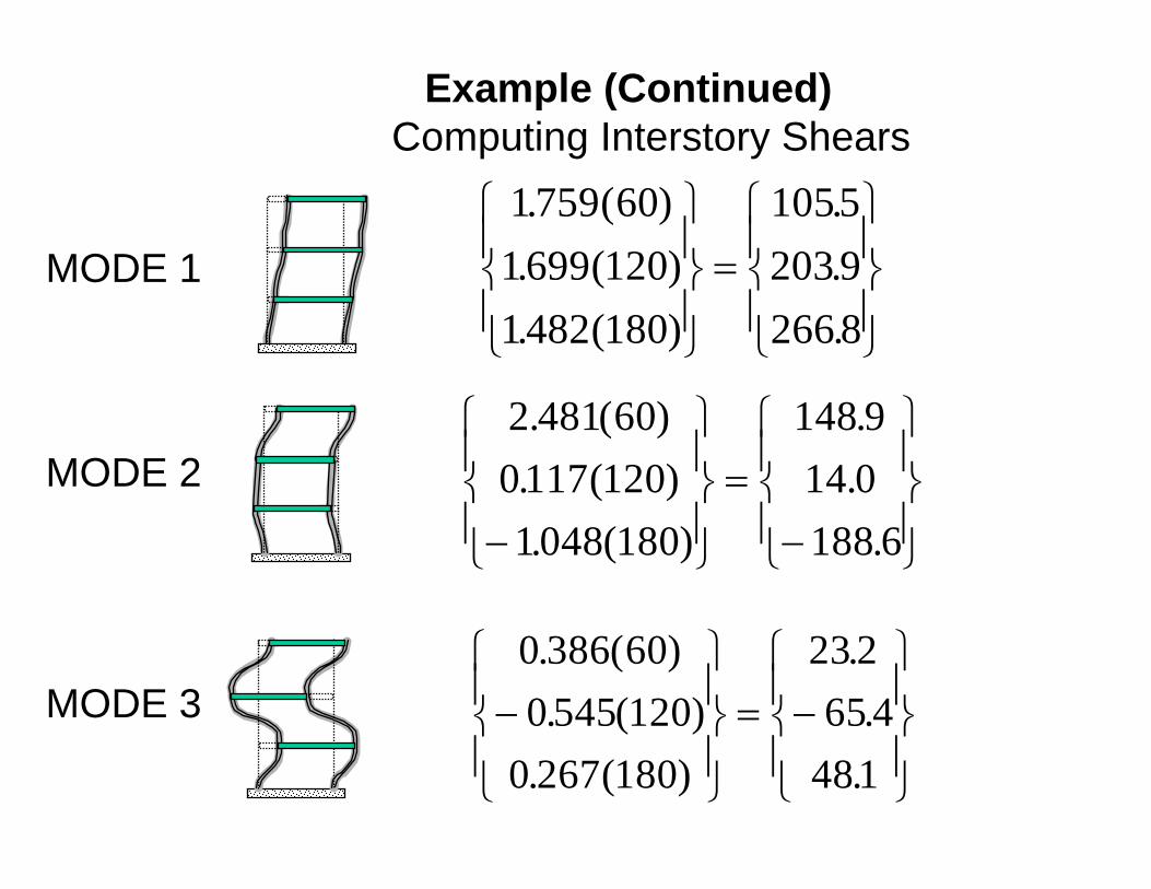
1759 601699 1201482 180
1055203 9266 8
. ( ). ( ). ( )
.
.
.
⎧
⎨⎪
⎩⎪
⎫
⎬⎪
⎭⎪=⎧
⎨⎪
⎩⎪
⎫
⎬⎪
⎭⎪
2 481 600117 1201048 180
148 914 0188 6
. ( ). ( ). ( )
..
.−
⎧
⎨⎪
⎩⎪
⎫
⎬⎪
⎭⎪=
−
⎧
⎨⎪
⎩⎪
⎫
⎬⎪
⎭⎪
0 386 600 545 120
0 267 180
23 265 4
481
. ( ). ( )
. ( )
..
.−⎧
⎨⎪
⎩⎪
⎫
⎬⎪
⎭⎪= −⎧
⎨⎪
⎩⎪
⎫
⎬⎪
⎭⎪
MODE 1
MODE 2
MODE 3
Example (Continued)Computing Interstory Shears
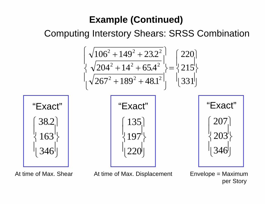
106 149 232204 14 654267 189 481
220215331
2 2 2
2 2 2
2 2 2
+ ++ ++ +
⎧
⎨⎪
⎩⎪
⎫
⎬⎪
⎭⎪=⎧
⎨⎪
⎩⎪
⎫
⎬⎪
⎭⎪
...
38 2163346
.⎧
⎨⎪
⎩⎪
⎫
⎬⎪
⎭⎪
“Exact”
At time of Max. Shear
135197220
⎧
⎨⎪
⎩⎪
⎫
⎬⎪
⎭⎪
“Exact”
At time of Max. Displacement
207203346
⎧
⎨⎪
⎩⎪
⎫
⎬⎪
⎭⎪
“Exact”
Envelope = Maximumper Story
Example (Continued)Computing Interstory Shears: SRSS Combination

-5
-4
-3
-2
-1
0
1
2
3
4
5
0 2 4 6 8 10 12
Time, Seconds
Mod
al D
ispl
acem
ent,
Inch
es
MODE 1MODE 2MODE 3
MODAL Response Time Histories:
Using Less than Full (Possible) Number of Natural Modes
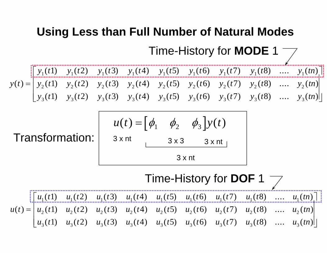
u tu t u t u t u t u t u t u t u t u tnu t u t u t u t u t u t u t u t u tnu t u t u t u t u t u t
( )( ) ( ) ( ) ( ) ( ) ( ) ( ) ( ) .... ( )( ) ( ) ( ) ( ) ( ) ( ) ( ) ( ) .... ( )( ) ( ) ( ) ( ) ( ) (
=1 1 1 1 1 1 1 1 1
2 2 2 2 2 2 2 2 2
3 3 3 3 3 3
1 2 3 4 5 6 7 81 2 3 4 5 6 7 81 2 3 4 5 6 7 83 3 3) ( ) ( ) .... ( )u t u t u tn
⎡
⎣
⎢⎢⎢
⎤
⎦
⎥⎥⎥
y ty t y t y t y t y t y t y t y t y tny t y t y t y t y t y t y t y t y tny t y t y t y t y t y t
( )( ) ( ) ( ) ( ) ( ) ( ) ( ) ( ) .... ( )( ) ( ) ( ) ( ) ( ) ( ) ( ) ( ) .... ( )( ) ( ) ( ) ( ) ( ) (
=1 1 1 1 1 1 1 1 1
2 2 2 2 2 2 2 2 2
3 3 3 3 3 3
1 2 3 4 5 6 7 81 2 3 4 5 6 7 81 2 3 4 5 6 7 83 3 3) ( ) ( ) .... ( )y t y t y tn
⎡
⎣
⎢⎢⎢
⎤
⎦
⎥⎥⎥
[ ]u t y t( ) ( )= φ φ φ1 2 3
3 x nt 3 x 3 3 x nt
3 x nt
Time-History for DOF 1
Time-History for MODE 1
Transformation:
Using Less than Full Number of Natural Modes
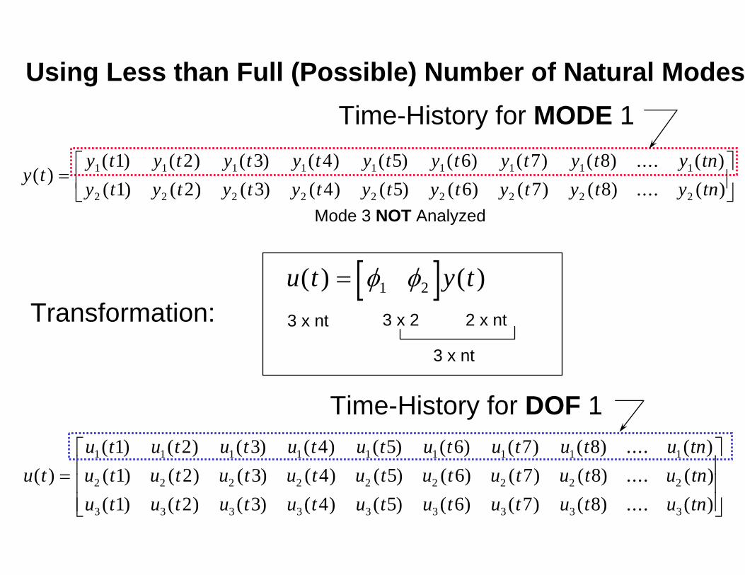
[ ]u t y t( ) ( )= φ φ1 2
3 x nt 3 x 2 2 x nt
3 x nt
Time-History for DOF 1
u tu t u t u t u t u t u t u t u t u tnu t u t u t u t u t u t u t u t u tnu t u t u t u t u t u t
( )( ) ( ) ( ) ( ) ( ) ( ) ( ) ( ) .... ( )( ) ( ) ( ) ( ) ( ) ( ) ( ) ( ) .... ( )( ) ( ) ( ) ( ) ( ) (
=1 1 1 1 1 1 1 1 1
2 2 2 2 2 2 2 2 2
3 3 3 3 3 3
1 2 3 4 5 6 7 81 2 3 4 5 6 7 81 2 3 4 5 6 7 83 3 3) ( ) ( ) .... ( )u t u t u tn
⎡
⎣
⎢⎢⎢
⎤
⎦
⎥⎥⎥
Time-History for MODE 1
Transformation:
y ty t y t y t y t y t y t y t y t y tny t y t y t y t y t y t y t y t y tn
( )( ) ( ) ( ) ( ) ( ) ( ) ( ) ( ) .... ( )( ) ( ) ( ) ( ) ( ) ( ) ( ) ( ) .... ( )
=⎡
⎣⎢
⎤
⎦⎥
1 1 1 1 1 1 1 1 1
2 2 2 2 2 2 2 2 2
1 2 3 4 5 6 7 81 2 3 4 5 6 7 8
Mode 3 NOT Analyzed
Using Less than Full (Possible) Number of Natural Modes
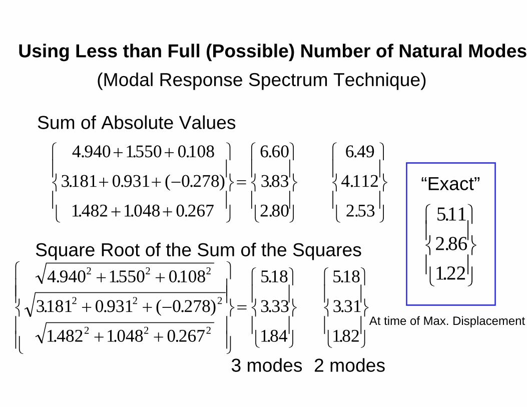
4 940 1550 0108
3181 0 931 0 278
1482 1048 0 267
518
333
184
518
3 31
182
2 2 2
2 2 2
2 2 2
. . .
. . ( . )
. . .
.
.
.
.
.
.
+ +
+ + −
+ +
⎧
⎨⎪⎪
⎩⎪⎪
⎫
⎬⎪⎪
⎭⎪⎪
=
⎧
⎨⎪
⎩⎪
⎫
⎬⎪
⎭⎪
⎧
⎨⎪
⎩⎪
⎫
⎬⎪
⎭⎪
Square Root of the Sum of the Squares
4 940 1550 0108
3181 0 931 0 278
1482 1048 0 267
6 60
383
2 80
6 49
4 112
2 53
. . .
. . ( . )
. . .
.
.
.
.
.
.
+ +
+ + −
+ +
⎧
⎨⎪
⎩⎪
⎫
⎬⎪
⎭⎪=
⎧
⎨⎪
⎩⎪
⎫
⎬⎪
⎭⎪
⎧
⎨⎪
⎩⎪
⎫
⎬⎪
⎭⎪
Sum of Absolute Values
5112 86122
.
..
⎧
⎨⎪
⎩⎪
⎫
⎬⎪
⎭⎪
“Exact”
At time of Max. Displacement
Using Less than Full (Possible) Number of Natural Modes(Modal Response Spectrum Technique)
3 modes 2 modes
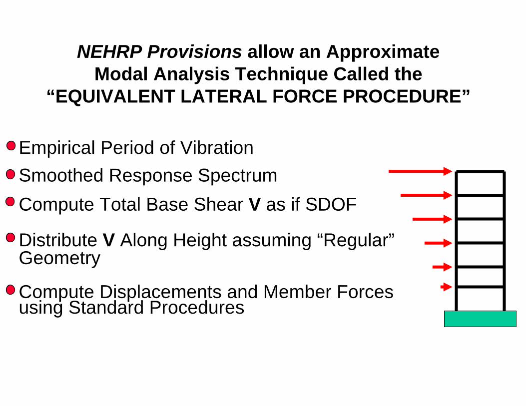
NEHRP Provisions allow an ApproximateModal Analysis Technique Called the
“EQUIVALENT LATERAL FORCE PROCEDURE”
Empirical Period of VibrationSmoothed Response SpectrumCompute Total Base Shear V as if SDOF
Distribute V Along Height assuming “Regular”Geometry
Compute Displacements and Member Forcesusing Standard Procedures


![6th Internationa] Modal Analysis ConferenceDamped Systems D. L. Cronin Modal Identities In Structural Dynamics 30-35 B. P. Wang Further Study On The Modal Damping Ratio Matrix For](https://img.pdfslide.us/doc/110x75/602214670d43a7149a27c0ef/6th-internationa-modal-analysis-damped-systems-d-l-cronin-modal-identities-in.jpg)