1

DAMP: a protocol for contextualising goodness-of-fit statistics in sediment-discharge

data-driven modelling

Robert J. Abrahart

1, Nick J. Mount

1, Ngahzaifa Ab Ghani

1,2, Nicholas J. Clifford

3 and Christian W.

Dawson4

1 School of Geography, University of Nottingham, Nottingham, NG7 2RD, UK

2 Faculty of Civil Engineering and Earth Resources, Universiti Malaysia Pahang, 26300 Kuantan,

Pahang Darul Makmur, Malaysia 3 Department of Geography, Kings College London, Strand Campus, Strand, London, WC2R 2LS,

UK 4 Department of Computer Science, Loughborough University, Loughborough, LE11 3TU, UK

Tel: +44 115 846 6145; Fax: +44 115 951 5249; Email: bob.abrahart@nottingham.ac.uk

Abstract

The decision sequence which guides the selection of a preferred data-driven modelling solution is

usually based solely on statistical assessment of fit to a test dataset, and lacks the incorporation of

essential contextual knowledge and understanding included in the evaluation of conventional

empirical models. This paper demonstrates how hydrological insight and knowledge of data quality

issues can be better incorporated into the sediment-discharge data-driven model assessment

procedure: by the plotting of datasets and modelled relationships; and from an understanding and

appreciation of the hydrological context of the catchment being modelled. DAMP: a four-point

protocol for evaluating the hydrological soundness of data-driven single-input single-output sediment

rating curve solutions is presented. The approach is adopted and exemplified in an evaluation of seven

explicit sediment-discharge models that are used to predict daily suspended sediment concentration

values for a small tropical catchment on the island of Puerto Rico. Four neurocomputing counterparts

are compared and contrasted against a set of traditional log-log linear sediment rating curve solutions

and a simple linear regression model. The statistical assessment procedure provides one indication of

the best model, whilst graphical and hydrological interpretation of the depicted datasets and models

challenge this overly-simplistic interpretation. Traditional log-log sediment rating curves, in terms of

soundness and robustness, are found to deliver a superior overall product — irrespective of their

poorer global goodness-of-fit statistics.

Key words: data-driven appraisal modelling protocol; data-driven model; neuro-fuzzy model; neural

network model; sediment rating curve; suspended sediment concentration; hydrological insight;

tropical catchment

1. INTRODUCTION

Accurate and reliable suspended sediment estimates are required in a variety of experimental and

operational hydrological situations, for scientific and/or river management purposes. Sediment ratings

may, for example, be used to estimate long-term rates of landscape denudation; to reflect river

morphological changes; to gauge sensitivity of catchments to varying land use practices; or for project

specific applications, such as the estimation of reservoir lifetimes, or in identification of tolerable

effluent discharge, and/or water quality inputs, around hydroelectric turbines. Accuracy and reliability

of such approaches are fundamentally limited: (i) by the quality and quantity of observations (both of

which, in turn, reflect sampling design and instrumentation); and (ii) by our ability (or otherwise) to

generalise site-specific fluxes to: larger catchment areas; contributing areas of catchments (which are

known to be highly variable); and/or event-specific and longer-term flow contributions (where various

hysteresis effects are frequently present). This may result in the use of multiple rating curves to

model different components of seasonal and hysteresis patterns, or in cases of highly complex

responses, it may necessitate the use of process-based models to adequately model the rating

relationship.

2

Conventionally, rating curves are generated from best fit regressions of suspended sediment — either

load (SSL) or concentration (SSC) — against river discharge (Q) or stage (H). Time-varying

behaviour may be captured by fitting two curves (where, for example, there is distinct seasonality in

sediment supply from a catchment), but where multi-scale temporal and spatial dependency is present

or required in the estimation, and/or when physical realism in the link between prediction and

predictor is required, then sediment concentration may be modelled as an output from one or more

inputs, distributed in time, space, or both. The data-driven model (DDM) offers an important

modelling paradigm in such respects, due to its central focus on identifying the computational

combination of multiple inputs according to the numerical structures found within a training dataset,

and the subsequent re-application of these captured structures to allow for prediction of incomplete

data series. Indeed, numerous examples of DDMs in hydrology that focus on suspended sediment

prediction have been reported over the last decade. These include individual or modular feedforward

neural network prediction (Cigizoglu, 2004; Jain, 2001; 2008); generalized regression neural network

prediction (Kisi, 2004a; Cigizoglu and Alp, 2006); radial basis function neural network prediction

(Kisi, 2004a; Alp and Cigizoglu, 2007); fuzzy-differential-evolution prediction (Kisi, 2004b: 2009);

neuro-fuzzy and fuzzy logic prediction (Kisi, 2005; Kisi et al., 2006); support vector machine

prediction (Cimen, 2008); genetic programming prediction (Aytek and Kisi, 2008); and neuro-wavelet

and neuro-fuzzy-wavelet conjunction model prediction (Partal and Cigizoglu, 2008; Rajaee et al.,

2010).

The number of published papers on suspended sediment prediction in rivers using DDMs is

increasing. However, long-standing criticisms that centre on the difficulties associated with generating

a physical interpretation of solutions that are commonly presented as an implicit black-box model

remain pertinent e.g. Minns and Hall (1996, p.400); Babovic (2005, p.1515); Abrahart et al. (2010).

Indeed, the ability of DDMs “to find connections between the system state variables (input, internal

and output variables) without explicit knowledge of the physical behaviour of the system”

(Solomatine et al., 2008; p.17) can lead to erroneous model conceptualisation and structure (Abrahart

et al. 2008) and issues of model equifinality (Beven, 2006; Todini, 2007). Moreover, model choice is

commonly justified on the basis of little more than qualitative appraisal of time series graphs, or

scatterplots of observed versus predicted records, plus a handful of global goodness-of-fit statistics.

This results in models that have little heuristic value beyond that of optimised curve fitting (Mount

and Abrahart, in press). Perhaps more dangerously, it may also result in the rejection of more complex

and/or more realistic solutions, in favour of simpler, unrealistic counterparts simply on the basis of

improved fit statistics (c.f. Oreskes, 2003). Two fundamental concerns therefore emerge:

1. There is an inherent risk in failing to properly understand or appreciate the complexities of a

particular dataset. Knowledge of the data quality, the likelihood of significant errors at

particular discharge ranges and the extent to which a solution may be influenced by outliers in

the dataset is vital.

2. There is a need for meaningful graphical inspections to be performed that assess the

appropriateness of each proposed and/or developed solution at different data ranges and with

respect to its hydrologic context.

Given these concerns, it is illuminating to contrast the decision making sequence commonly adopted

by sediment-discharge data-driven modellers with those engaged in more conventional, empirical

modelling approaches and, for whom, the need to provide both hydrological and physiographical

context for their results has long been recognised e.g. following the well-established protocol of

Glysson (1987). Figure 1 shows the two sequences. The DDM decision sequence is highly simplistic

and reliant on statistical fit information to guide the selection of the preferred model. Indeed, it

clearly exemplifies the key assumption underpinning data-driven approaches: that the modelling

mechanism will learn the required knowledge directly from the data and, in so doing, deliver a

preferred model without the need for a priori understanding of either data or hydrological context. By

contrast, conventional empirical model decision sequences use contextual understanding to guide the

constraints that should be incorporated into a model (i.e. linear, power function) and evaluate model

3

outputs in terms of both form and fit to the data. In so doing, a more meaningful feedback loop is

incorporated, through which valuable diagnostic information about the model form and fit is used as

an additional piece of evidence to: (i) deliver an enhanced understanding of the scientific challenges

involved and; (ii) assist thereafter in helping hydrological modeller’s to refine their products.

One approach to addressing the above concerns is through improvement of the DDM decision making

sequence so that contextual hydrological and data-quality-related understanding is more fully

incorporated, with the result that the DDM and conventional empirical decision sequences are more

closely mapped. However, this raises the crucial question of how to include and use contextual

information to improve model evaluation, whilst adhering to the notion that the data-driven modelling

mechanism should be allowed to generate models directly from the data, in the absence of additional

knowledge inputs (i.e. external contextual material should not be allowed to act as an a priori guide

that is acquired from the modeller). A simple solution is presented in Figure 2. Parallel knowledge

about model form and fit, and an understanding of the modelling problem and the hydrological

dataset, are conflated and used to guide the preferred model selection. Crucially, contextual

understanding of the data is included in the post-modelling phase of the decision sequence; thereby

enabling it to be used in the model selection process whilst ensuring that it does not form a

preconceived initial input into the data-driven modelling mechanism.

The decision sequence in Figure 2 can be recast to a four-point data-driven appraisal modelling

protocol (DAMP). This protocol mimics the classic empirical approach of Glysson (1987) and asserts

that the development of DDM solutions for modelling sediment-discharge relations requires the

following actions:

1. At the outset, the data are assessed in terms of their physiographic and hydrologic context so

that clear hypotheses about the spatial and temporal processes that are expected to be driving

suspended sediment over the period of the dataset are developed;

2. The data are examined and reported in depth. The purpose of this analysis is to fully disclose

its quality and evidential errors;

3. A synthesis of the main hydrological processes driving the sediment / discharge relationship

in the catchment is used to inform an explanation of the resultant structures that one can

observe in a standard log-log plot of the paired dataset;

4. The data are next modelled and, if permitted, explicit formulae thereafter developed to

represent each model. Each equation is subsequently used to develop and present a

regularised data series, from which the performance of each individual solution is examined

within its hydrological context and across its data ranges. Finally, the difference in each

model’s ability to predict suspended sediment in these ranges is identified, and the best

performing model is selected on the basis of both goodness-of-fit statistics and the extent to

which the model form reflects the catchment’s hydrological context and avoids being overly

influenced by data quality issues.

Points 1-3 should be easily achieved in all data-driven modelling scenarios. Point 4 raises a significant

challenge as many data-driven modelling mechanisms are presumed to be of an ‘implicit nature’.

However, numerous DDM solutions can be made explicit, by adjusting software settings, or by means

of some minor re-coding, such that their internal structures and parameters can be extracted/exported

and reported/shared. For example, Lee et al. (2006) provided a neural network (NN) equation for

estimating reservoir sedimentation due to typhoon events in Taiwan; Aytek et al. (2008) provided a

NN equation for estimating daily reference crop evapotranspiration in California, USA – albeit that

the correctness of the latter has been placed in doubt (Abrahart et al., 2009). The alternative but less

attractive option in such cases is to simply run a regular series through each original computer model

and publish that paired input-output sequence in a spreadsheet. For those DDMs which do offer

explicit outputs, the opportunity to assess the appropriateness of the solution in the context of DAMP

is greatly enhanced. For example, in the case of neuro-fuzzy (NF) modelling, it is claimed that "the

additional benefit of being able to provide the set of rules on which the model is based ... gives further

insight into the process being modeled" (Sayed et al., 2003; p.123: reproduced in the closing

4

paragraphs of Kisi, 2005; Kisi et al., 2008, 2009). Consequently, the appropriateness of a NF model’s

computational structures and rules, may be reasonably assessed by means of detailed referencing and

comparison against two independent sources: (i) the structures that can be visualised in the data; and

(ii) our domain knowledge of the physical or operational and mechanical processes that are

responsible for such structures.

For sediment-discharge rating curves, saved in proprietary model format, or converted into explicit

equations it is possible to apply DAMP in full by throughputting an ordered, regular series of inputs,

spanning the range of the input predictor values required, and plotting model outputs as an organised

sequence of points. Whilst undertaking analyses of this type is unusual, it is not new and a small

number of under-appreciated exemplars already exist e.g. the two fuzzy modelling rainfall-runoff

relationships plotted in Şen and Altunkaynak (2003; p.42). Indeed, for simple DDMs where the

number of predictor variables is low (most sediment-discharge models are of this type), 2D modelled

relationships can be depicted using bi-variate plots and 3D modelled relationships can be mapped as

surfaces.

In this paper, just such an approach is adopted and we exemplify DAMP by means of a re-evaluation

of seven explicit models used to predict SSC from Q for a small tropical catchment in Puerto Rico.

The purpose here is not to offer direct insights into better model development strategies, but to

highlight the dangers associated with data-driven model selection made on the basis of summary

goodness-of-fit statistics alone. Consequently, this paper provides an important foundation/ blueprint

for those wishing to present sediment-discharge DDM models in such a way that are better able to

respond to the ‘black-box demonization’ that has plagued them, to date, and in so doing, integrate

contextual hydrological and data-related information into model selection and evaluation. The clear

weaknesses that have surrounded the use of goodness-of-fit statistics to assess model performance are

mitigated and a case for the greater acceptability of DDMs in hydrological modelling is presented. In

addition, calls for increased accessibility and portability of hydrological applications (Buytaert et al.,

2008; Abrahart et al., 2009) are heeded and the explicit equation for each model in this paper is

reproduced and encoded in a spreadsheet for third parties to use in experimental operations (Appendix

1: Supplementary Material).

2. STUDY SITE AND DATASETS: PHYSIOGRAPHIC, HYDROLOGIC AND

SEDIMENTOLOGIC CONTEXT

2.1. The study site

The modelling scenario is one of the two independent case studies that were investigated in Kisi

(2005): estimation of United States Geological Survey (USGS) SSC records for upper reaches of the

'Rio Valenciano near Juncos', situated on the island of Puerto Rico, in the Caribbean (USGS Station

No. 50056400: Figure 3). The sediment budget at this gauging station is of particular hydrological

modelling interest since the Commonwealth of Puerto Rico, Aqueduct and Sewer Authority are

constructing a 30m high dam on this river to meet increased water demand: situated about 2 km south

of the city of Juncos (http://www.csagroup.com/project.php?msid=1&pid=40).

The USGS monitoring site is located at an elevation of approximately 70 m, roughly halfway between

the river’s source in the hills above Las Piedras, and the confluence of the Rio Valenciano and Rio

Grande de Loiza in the alluvial plains of the Cagus-Gurabo-Juncos region. The catchment area above

the gauge is 42.4 km2 and rises to approximately 400 m at its highest point. The river flows through

mainly suburban land use for about 7 km immediately upstream of the gauge (Pares-Ramos et al.,

2008) where a relatively low relief landscape is characterised by a mix of grassland and low density

urban development. This land use changes to a rural classification in the uppermost sub-catchments.

In common with the majority of upland rivers on this island, the rural upland reaches of the Rio

Valenciano are highly incised and bedrock controlled. Floodplains are generally poorly developed and

the channel is commonly highly connected to the valley sides; resulting in few opportunities for out-

of-channel sediment storage. Forestry remains the primary land use type on the steepest valley sides

and in the highest elevation first order sub-catchments. Much of the upland catchment has however

5

been deforested: a process resulting in the replacement of natural forests by grassland, shrub land,

arable agricultural land or plantations (Helmer et al., 2002; Pares-Ramos et al., 2008). Elevated ridges

in the upper reaches are characterised by low density urban development.

This catchment is one the many northward draining examples on the island that are characterised by

high mean annual rainfall of between 2000 and 2500 mm yr-1

(Larsen and Torres-Sanchez, 1998),

moderate to high annual sediment yields and moderate to high annual runoff (Warne et al., 2005).

Rainfall is temporally variable with low-intensity localised rainfall events tending to be fairly evenly

distributed throughout the driest months of the year (January to April); resulting in a persistent low-

level base flow in the majority of northern catchment channels. By contrast, mean rainfall doubles

during the wetter months of May to October and, in some larger catchments, such rainfall can result in

sustained moderate discharges. The island also experiences occasional, extreme rainfall-runoff events

associated with hurricanes that recur over 10-20 year periods (Ho, 1975; Nueman et al., 1990; Scatena

and Larsen, 1991). Indeed, although infrequent, hurricane-related events are important for generating

sediment, with 285 shallow landslips reported by Scatena and Larsen (1991) in upland forested

valleys during the passage of Hurricane Hugo (1989). The upper Rio Valenciano catchment for

example was classified as having moderate landslide susceptibility by Larsen and Torres-Sanchez

(1998). The remaining winter months are dominated by localised high intensity rainfall events linked

to annually-recurring winter frontal storms. Major storms are intense but brief and in response most

catchments on the island exhibit very flashy hydrological regimes in which maximum discharges can

be up to four orders of magnitude above base flow, yet recede over hours, or at most a few days

(Warne et al., 2005). In consequence, the occurrence of high sediment yields in northern catchments is

often episodic with the highest sediment concentrations related to short-lived flood events associated

with storms and landslides.

There are no detailed geomorphological and physiographic studies of the catchment available in the

literature, although studies in the nearby Luquillo Mountains (USGS, 2000) provide the best

contextual data available for its upland reaches. It is, therefore, not possible to a priori suggest either:

(i) a definitive sediment budget; or (ii) specific elements of a sediment yield/delivery system (Dunne,

1979). Indeed, in a study of small basins in Puerto Rico, Larsen (1997) drew attention to marked local

variability in basin response, which reflected catchment physiography; underlying geology; history of

land use, and/or past and present land use clearance; and adjustments of the stream network with

respect to local sediment storages in bar forms, and to channel-hillslope interactions. It follows from

this, that any dataset must be closely tied both to the particular basin under consideration and to the

position of the measuring station in relation to the stream network – since the influence of very local

network sediment storages and supplies may be evident in any data records. However, comprehensive

studies of other northern catchments on the island (e.g. Larsen, 1997; Larsen and Torres-Sanchez,

1998; Warne et al., 2005; Diaz-Ramirez et al., 2008) do allow the general characteristics of sediment

dynamics to be posited. These indicate that a high degree of seasonality in sediment erosion, and

hence of sediment supply to the stream network, is to be expected in conjunction with a rapid transit

of suspended sediment through the upland stream network. The effect may be complicated (probably

compounded) since the 'hurricane season' also corresponds with the wettest months i.e. the largest,

most intense precipitation events, coincide with an already wet period. Event-specific highs in

sediment yield associated with landslides and localised soil erosion — if present — could thus be

superimposed on higher, seasonal values. The presence of ‘extreme’ values, is, therefore, to be

expected, and such occurrences may well have a disproportionately large influence on sediment

transport and suspended sediment concentration in relation to their frequency of occurrence.

However, given the small size of most catchments on this island, it may also be the case that seasonal

effects are further complicated by local variations in sediment availability, if not delivery: large

rainfall events early in the wetter season might, therefore, be expected to produce a higher sediment

yield than events occurring later in the season, when more of the available sediments have been

eroded. However, this will depend upon local land stability conditions and any changes in land use

practice. Some upper-end tailing-off or dipping of rating curves might also, then, be anticipated. The

net effect of all of the above might most likely be encountered in the portrayal of a two- or multi-stage

log-log regression relationship, between sediment concentration and discharge (principal seasonal

6

effect). That relationship might also be expected to exhibit differing levels of scatter about the

individual stages: (i) as a result of event-specific factors; (ii) due to extrapolation and infilling of

missing records: or (iii) associated with different types of hysteresis, where similar sediment

concentrations are recorded for very different discharges (Williams, 1989).

2.2. The datasets

Full particulars for the monitoring station at Rio Valenciano near Juncos are provided in Table 1.

Following Kisi (2005), paired time series datasets comprising daily river discharge (Q in m3 s

-1) and

daily SSC (S in mg l-1

) records for 1 October 1993 - 30 September 1995 were downloaded from the

USGS open access website at: http://webserver.cr.usgs.gov/sediment (Figure 4).

Little additional metadata is available from the download site, so additional information related to

gauge instrumentation, and any data processing or infilling, was requested directly by the authors

(Carlos Figueroa-Alamo, USGS, PR, pers. comm.). This request revealed that SSC records for low to

moderate discharges were collected using a manual depth-integrated sampler. For high discharges an

automatic sediment sampler with liquid level actuator (non-depth integrated) was used. Sampling

frequencies are not disclosed. Importantly, it is also revealed that field-based SSC sampling was not

continuous and that data infilling was necessary for some SSC records; particularly those at low

discharges. The methods by which this infilling was accomplished are not detailed. Similarly, for the

highest discharges SSC is extrapolated via rating curves; but the form and reliability of these curves

remains unclear.

The raw dataset is presented as a log-log plot in Figure 5. The observed sediment-discharge

relationship, could obviously be reasonably-well captured by means of log-log regression, with

varying degrees of scatter due to seasonal and/or event-specific factors, and exhibiting a general

reduction in the gradient of the curve in the uppermost ranges of the dataset (limited sediment

availability). However, a number of important additional structures can also be observed. The degree

of scatter associated with the four extreme discharge events (>15 cumecs) is relatively low and the

expected high degree of heteroscedasticity in the dataset may be artificially constrained by the

application of upper-magnitude extrapolation procedures. The scatter of points below 0.5 cumecs is

characterised by numerous horizontal ‘lines of points’ (A); implying that SSC is constrained to only

one of seven or eight possible values. Each particular value also occurs across a range of overlapping

discharges. Clearly, such records are not realistic. This regular pattern is most likely an artefact

arising from measurement and recording imprecision at very low levels of SSC i.e. discretisation/

round-off. It could even, perhaps, be an unintended by-product of missing record “infilling

operations”. This particular activity was mentioned in the personal communication and might help in

part to explain the extent of their horizontal spread. Contrasting vertical ‘lines of points’ (B) also exist

in the data between 0.5 and 0.8 cumecs; suggesting that wide ranges of SSC values have been

recorded for identical discharges. Again, this is highly unlikely, and one may reasonably presume that

these structures are due to a reduced precision in the discharge record that has resulted in SSC data

being assigned to one of a small number of data ‘bins’. Two significant outliers also exist (O1 and

O2) whose validity it is difficult to imagine: 24 April 1994 (Flow = 0.0906 m3 s

-1; Sediment = 1200

mg l-1

) and 6 June 1994 (Flow = 0.2270 m3 s

-1; Sediment = 312 mg l

-1). Indeed, the most likely

explanation for these peculiarities is data error in the source material.

This initial appraisal of the dataset, coupled with the physiographic, hydrologic and sedimentologic

context, raises some important issues for those wishing to generate a DDM of suspended sediment for

the Rio Valenciano. First, the data frequency (daily mean) does not correspond with the expected

hydrological event frequency (commonly less than 24 hours); potentially resulting in a significant

underestimation of the instantaneous 'peak value' for SSC in cases of a rapid and/or larger event.

Second, using data extrapolation procedures for high discharges may be problematic, since it results

in records that do not adequately capture the variability of the sediment supply and transport processes

that occur within a catchment under extreme conditions. Consequently, the occurrence of extreme

events in the dataset may be constrained. Given the fact that majority of suspended sediment yield in

northern catchments is associated with flashy, high discharge events, this also raises questions over

7

the usefulness of such time series records for modelling SSC. Moreover, the relatively simple form of

most rating curves, can easily be replicated by most DDMs, such that the vast majority of resultant

models will appear to possess high levels of skill if assessed in terms of goodness-of-fit statistics;

thereby giving a false indication of the validity of the model at high discharges. Third, clear

shortcomings exist with regard to measurement and recording precision of SSC. This has resulted in a

record that fails to properly represent a tight sediment-discharge relationship at low discharges. The

combined depiction of inappropriate scatter and artificial structures moreover delivers a substantial

amount of uncertainty as to what does or does not constitute a correct answer in that region. The

extent to which such particular imperfections could have a detrimental impact on a potential solution

is nevertheless open to question: it may have little operational relevance for the resultant model, since

the contribution to overall suspended sediment loads from low discharges is likely to be minimal.

However, given the higher frequency of low discharge records in each dataset, a large proportion of

the data used to train a DDM may not be representative of real suspended sediment behaviour, such

that the ability of the model to produce realistic predictions at low discharges may be impaired.

Finally, the existence of the two outliers in the data are likely to encourage a general over-estimation

of SSC at discharges < 1 cumec.

3. METHODOLOGICAL APPROACH

The underlying methodology is that of Kisi (2005); extended as required to support a more

comprehensive analysis by means of DAMP:

1. Download dataset and divide it into two subsets: (Set A) and (Set B);

2. Develop a number of DDMs on Set A and test on Set B (Experiment 1);

3. Develop a number of DDMs on Set B and test on Set A (Experiment 2);

4. Extract each model’s rules, weights, parameters and governing equations (as required);

5. Use these rules to develop and present a regular data series such that the modelled relationship

between SSC and Q can be plotted as a continuous curve;

6. Compare goodness-of-fit statistical performances for all models using the two contrasting

datasets;

7. Examine how well each regular curve performs with respect to its hydrological context in

particular ranges of the original dataset; as outlined above.

The downloaded material was first divided into two equal and consecutive subsets. Set A (Kisi’s

training dataset) contained 365 paired daily values for the 1994 water year (1 October 1993 - 30

September 1994); Set B (Kisi’s testing dataset) contained 365 paired daily values for the 1995 water

year (1 October 1994 - 30 September 1995). Earlier studies, however, had included a lagged input of

1-day: meaning that no prediction could be delivered for 1 October. This necessitated removal of the

observed record for 1 October 1993 from Set A and 1 October 1994 from Set B: leaving 364 records

in each set. Table 2 provides a statistical description of each variable in each final subset and a

number of single measurement inequalities can be identified. The highly skewed and highly peaked

nature of discharge and sediment in both catchments should be emphasised. Table 2 also reveals

potentially problematic differences in the split of observed records that could create a substantial

impact on overall outcomes. The split-distribution is not well balanced: the calibration and testing

datasets possess marked disparities in terms of mean, skewness and kurtosis. The extent to which

relational or covariant inequalities might be an issue is not revealed in such descriptors. Last, but by

no means least, no error checking, outlier removal or data cleansing operations were reported in the

original paper and so the assumption must be that none of the original downloaded records should be

deleted. Consequently, the two erroneous outliers remained.

To allow direct comparison with Kisi’s earlier paper the four models that he reported are replicated

here. These are a neuro-fuzzy model possessing triangular membership functions (NFT); a neural

network model possessing a linear transfer function in its output unit (NNL); a traditional power

function sediment rating curve model (PFT) and a simple linear regression model included for the

purposes of 'linear benchmarking' (SLR). In addition we also present results from a neuro-fuzzy

8

model possessing Gaussian membership functions (NFG); a neural network model possessing a

nonlinear transfer function in its output unit (NNN) and a bias-adjusted power function sediment

rating curve model (PFA). Therefore, a total of seven separate modelling approaches are presented.

In accordance with the approach adopted in Kisi (2005), each of the seven independent models was

calibrated on data Set A and tested on Set B, identified by means of a prefix attached to each model,

in this case 'MOD'-1 This scenario allowed direct comparison between the numerical assessment

statistics presented in the earlier paper and the establishment of some measure of correspondence, or

fidelity, in terms of replication with regard to the recreation of earlier reported solutions. However, in

addition, we also adopted a 'role reversal test' by comparing and contrasting models calibrated on Set

B and tested on Set A ('MOD'-2). The object of this particular exercise was to test for a consistent

response, since from earlier discussions, it was suspected that disparities related to the original

selection of appropriate subsets for calibration and testing purposes could be influential and had

perhaps led to a unique set of findings. Consequently, 28 sets of numerical predictions are reported for

subsequent out-of-sample assessment in terms of conventional statistical methods.

Three methods of reporting are adopted. Each model comprises an explicit set of mathematical rules

and/or equations that can be used to describe the form of the relationship and in so doing will provide

an exact method, for comparing and contrasting the different types of solution, which is also

transparent. The equations are provided below and in the accompanying spreadsheet (Appendix 1:

Supplementary Material). Having both computational and mathematical models at our disposal means

that it is possible to obtain outputs for a regular series of pre-specified discharge inputs, in this case

ranging from some practical minimum [0] to some upper operational limit [50] that exceeds the

maximum observed record [35.1] for Q. The resultant outputs can thereafter be plotted as a

continuous function for visualisation purposes in the same manner as a simple linear regression

equation overlaid on the original scatterplot of observed S vs. observed Q. The extent to which each

model fits the dataset can thereafter be inspected for hydrological correctness. Particular emphasis

should be placed upon: (i) the development of a flexible nonlinear response, accommodating local

deviations from the global trend; and (ii) the treatment of outliers. The use of an extended series that

is expanded well beyond the upper range of the observed dataset is particularly useful in exploring the

extrapolation capabilities of each model that was produced. Individual model outputs were also

compared and contrasted against one another by means of seven popular metrics computed using

HydroTest (www.hydrotest.org.uk): an open access web site that performs the required numerical

calculations in a standardised manner (Dawson et al. 2007; 2010). The selected statistics comprised:

three absolute measures — Mean Absolute Error (MAE), Mean Error (ME) and Root Mean Squared

Error (RMSE); three relative measures — Mean Absolute Relative Error (MARE), Mean Relative

Error (MRE) and Mean Squared Relative Error (MSRE); and one dimensionless coefficient — R-

Squared (RSqr). Full details with regard to the calculation and use of such descriptors, are provided in

the aforementioned papers. Table 3 contains formulae for and descriptions of all seven metrics: noting

that signed statistics are reported as a residual, not an error, such that a positive residual equates to a

negative error. The total annual sediment flux for each model and period is also of interest and was

calculated separately in metric tons per water year. It is reported in percentage format as Total Error

(TE): a measure that is signed according to error, not residual. In practical terms TE provides a

simple, but nevertheless very useful, additional statistic: one that places added weight on higher

flows/concentrations. This particular weighting is especially important, given that events of this

nature will make a significant contribution in terms of overall yield, and that issues surrounding the

latter are what many, if not most, practitioners are mainly concerned about.

4. MODELLING OPERATIONS

9

4.1 Neuro-Fuzzy Models

Neuro-fuzzy modelling was performed in MATLAB using the Adaptive Neuro-Fuzzy Inference

System (ANFIS: Jang, 1993; Jang et al., 1997). Kisi (2005) employed triangular membership

functions in all reported applications. That original analysis is extended in this paper to encompass an

assessment of two different internal membership functions: triangular and Gaussian. NF models

containing either one or other type of internal membership function were developed to meet the

demands of each individual experiment. Each NF model involved was designed to be consistent with

the best performing NF solution of Kisi (2005). No pre- or post-processing operations were applied.

Each model used one raw input, to deliver one raw output, and contained two internal membership

functions – as depicted in Figure 6. This is the simplest possible model that the software package will

support. It also means that only two rules and two pertinent, appropriately weighted linear output

equations will be produced; delivering one internal rule for each of the two individual input

membership functions involved. Kisi (2005) did not report the training period or stopping condition

that was used to develop his NF model; our assumption, under such circumstances, is that his models

were trained for 10 iterations — this number comprising a default setting in the MATLAB Fuzzy

Logic Toolbox. Testing was nevertheless performed to ascertain the correctness of our model fitting

activities, since it is possible that the resultant solutions could be either underfitted or overfitted.

Figure 7 depicts regular series outputs for NF models developed using a limited set of different

iteration settings: starting at 5 (half of default), and thereafter doubling to 10 (default), 20 and 40.

NFT-1 and NFT-2 outputs revealed a progressive process of continued adjustment, such that

additional iterations delivered a series of substantial modifications causing each NFT model to

provide very different high-end output trajectories at different stages of the training process. The need

to perform some sort of 'early stopping' operation is thus indicated, perhaps founded on the prudent

use of a cross-validation dataset. However, such considerations and procedures are not part of the

original published methodology, and so regardless of other factors the default number of iterations

was applied in our final modelling exercises. NFG-1 and NFG-2 outputs in contrast depicted limited

overall changes and a more 'stable solution': such that the use of default settings could not as a result

be faulted.

For each finished product, the software package provided modelling parameters for two fitted

membership functions, enabling the relevant internal weights to be calculated. It also produced a set

of rules and for each rule it supplied a linear output equation. Full particulars are listed in Table 4. The

two rules are quite simple and are combined in the region of 'membership function overlap' — as

depicted in Figure 8. Thus:

Rule 1: If Q is MF1 then S is S1

Rule 2: If Q is MF2 then S is S2

Rule 3: If Q is MF1 and MF2 then S is S1 + S2

It is also possible to demonstrate in an exact manner how our modelling outputs can be computed

using the information that is provided in Table 4. The calculation of model output (S) can be

simplified into a three-step procedure:

1) Calculation of weights. The membership score (weight) for each input is obtained using the

parameters listed in Table 4. For NFT the triangular curve is a function of vector Q, and depends on

three scalar parameters a (left foot), b (peak), and c (right foot). From these parameters, the weight of

each rule (Wi) is calculated as:

If Q ≤ a then Wi = 0 (1)

If a ≤ Q ≤ b then Wi = (2)

10

If b ≤ Q ≤ c then Wi = (3)

If Q ≥ c then Wi = 0 (4)

whilst for NFG, the weight of each rule (Wi) is calculated as:

Wi =

(5)

The weight for each rule is thereafter normalised i.e. divided by the 'sum of weights'. For example, the

normalised weight for Rule from number of rules is calculated as:

(6)

2) Calculation of sub-outputs. The linear function related to each particular rule is next multiplied by

its corresponding normalised weight e.g., , …. . This step weights the

strength of each rule and provides sub-output to the final output.

3) Calculation of final output. The sub-outputs are thereafter summed to provide the final output:

(7)

For example, S at Q = 0.425 in NFT-1 is calculated as follows:

(8)

where

and where a, b and c are values listed in Table 4.

4.2 Neural Network Models

Neural network modelling was performed using an in-house software program that has delivered

sound performance on several previous occasions e.g. Dawson et al. (2002; 2006). Kisi (2005)

employed a linear output transfer function in all reported applications. This is the default setting in

MATLAB. That original analysis is extended in this paper to encompass an assessment of two

different output transfer functions: linear and nonlinear. NN models containing either one or other

type of output transfer function were thus developed to meet the demands of each individual

experiment. Each NN model involved was designed to be consistent with the best performing NN

11

solution of Kisi (2005). Each model used one raw input, to deliver one raw output, and contained one

hidden unit — as depicted in Figure 9. Each NN model was trained using 'back propagation with

momentum' for 10,000 epochs: for a detailed account of relevant neurocomputing terms and

procedures see Priddy and Keller (2005). This is the simplest hidden-unit architecture permitted. Kisi

(2005) did not report his training parameter settings or, indeed, if some method of standardisation

should be applied to either the input or output datasets. Thus we opted to use a tried and tested

approach, that had been used successfully on a number of previous occasions, comprising: a training

rate of 0.1, a momentum setting of 0.9, and datasets standardised to range from 0.1 to 0.9. To support

operational considerations, each model run was performed in a blind manner, requiring both training

and testing datasets to be standardised to the range of the training dataset.

The two NNL and two NNN models can be explained, using a sequence of equations. Figure 9 depicts

the NN architecture that was adopted, comprising one unit in the input layer (i), one unit containing a

'sigmoid activation function' in the hidden layer (j), and one unit that could contain either a linear

activation function (as shown) or a sigmoid activation function (not shown) in the output layer (j). No

processing occurs in the input layer. Inputs are simply passed to the hidden layer in which the

processing operation delivers outputs (Sh) using a sigmoid transformation in accordance with

Equation 9.

(9)

where Qstd is obtained using Equation 10.

(10)

Sh is thereafter passed to the output layer, and processed according to one or other of the two potential

transformations, linear or non-linear. Final output for NNL is calculated using Equation 11; final

output for NNN is calculated using Equation 12.

(11)

(12)

where Sstd is then de-standardised back to the original scale by Equation 13 to get the final output S.

(13)

Trained parameter settings obtained for Equations 9 to 13 are provided in Table 5.

4.3 Sediment Rating Curves

Two established statistical solutions were developed in Microsoft Excel: a traditional sediment rating

curve (PFT) and a bias-adjusted sediment rating curve (PFA). The sediment rating curve method is

attributed to Campbell and Bauder (1940) who observed that the relationship between the logarithm

of sediment concentration and the logarithm of discharge is approximately linear. PFT is a

straightforward least squares linear regression model of log S on log Q. Equation 14 depicts this

relationship in the form of a power function where a and b are constants acquired during the

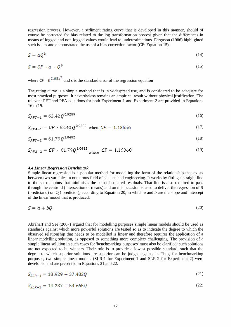
12

regression process. However, a sediment rating curve that is developed in this manner, should of

course be corrected for bias related to the log transformation process given that the differences in

means of logged and non-logged values would lead to underestimations. Ferguson (1986) highlighted

such issues and demonstrated the use of a bias correction factor (CF: Equation 15).

(14)

(15)

where CF = and s is the standard error of the regression equation

The rating curve is a simple method that is in widespread use, and is considered to be adequate for

most practical purposes. It nevertheless remains an empirical result without physical justification. The

relevant PFT and PFA equations for both Experiment 1 and Experiment 2 are provided in Equations

16 to 19.

(16)

where (17)

(18)

where

(19)

4.4 Linear Regression Benchmark

Simple linear regression is a popular method for modelling the form of the relationship that exists

between two variables in numerous field of science and engineering. It works by fitting a straight line

to the set of points that minimises the sum of squared residuals. That line is also required to pass

through the centroid (intersection of means) and on this occasion is used to deliver the regression of S

(predictand) on Q ( predictor), according to Equation 20, in which a and b are the slope and intercept

of the linear model that is produced.

(20)

Abrahart and See (2007) argued that for modelling purposes simple linear models should be used as

standards against which more powerful solutions are tested so as to indicate the degree to which the

observed relationship that needs to be modelled is linear and therefore requires the application of a

linear modelling solution, as opposed to something more complex/ challenging. The provision of a

simple linear solution in such cases for 'benchmarking purposes' must also be clarified: such solutions

are not expected to be winners. Their role is to provide a lowest possible standard, such that the

degree to which superior solutions are superior can be judged against it. Thus, for benchmarking

purposes, two simple linear models (SLR-1 for Experiment 1 and SLR-2 for Experiment 2) were

developed and are presented in Equations 21 and 22.

(21)

(22)

13

5. RESULTS

5.1. Model comparison with original study

Three metrics reported in Kisi (2005) can be used to deliver an objective comparison for the purpose

of ascertaining the overall extent to which our one-input one-output NFT-1 and NNL-1 models are

analogous to their published equivalents (Table 6). The original models were assessed on Mean Root

Squared Error (MRSE), RSqr and TE. MRSE is computed from RMSE according to Equation 23.

(23)

where n is the number of records, which is 364. TE was labelled “relative error” in the previous paper.

The statistical results are quite similar, as expected. The original NFT-1 and NNL-1 models

nevertheless exhibit marginal albeit inconsistent overall superiority to their latest replicated

counterparts. It is impossible to establish to what extent the observed discrepancies can be attributed

to random processing elements such as the use of different architectural initialisations or

computational precisions. The underlying similarities are nevertheless sufficient to corroborate the

key findings of Kisi (2005). These are:

1. statistics for NFT-1 are slightly better than those for NNL-1,

2. PFT-1 and SLR-1 do not perform as well as the other two models.

5.2. Statistical metrics

Table 7 contains a full set of output evaluation statistics for Experiment 1. NN and NF solutions

provided somewhat similar measures of global fit, to the extent that there might be no significant or

meaningful statistical difference occurring, between each individual model, especially in the training

situation. Numerical results, for fitting models to the training dataset, are mixed — with no clear

winner emerging. NN models are perhaps superior. NNL-1 had a slight advantage in terms of MAE.

NNN-1 had an even narrower advantage in terms of RMSE. RSqr was identical in all four cases.

NFT-1 and NFG-1 had zero ME meaning that such models were unbiased. Testing, as might be

expected, provided similar measures of statistical fit for NN and NF solutions but with NFT-1 on this

occasion doing somewhat better than the others on MAE, ME, RMSE and RSqr. The assumption in

such cases, if one is possible, is that lower training performance of NFT-1 on Set A resulted in

superior generalisation performance on Set B; whilst the tighter fit that NNL-1 and NNN-1 achieved

on training Set A, handicapped the transfer of such modelling solutions, in terms of their fit to Set B.

This interpretation of matters, however, is to some extent contradicted by the fact that NNN-1

returned the top score for TE: conceivably making it the practitioner’s choice.

Table 8 contains a full set of output evaluation statistics for Experiment 2. The statistical results

obtained using role reversal, are somewhat different, to that reported for Experiment 1. Three out of

four NN and NF solutions provided similar measures of global fit. NNL-2, surprisingly, performed a

great deal worse than the other models. Further investigation revealed that this minimalist model

lacked sufficient internal flexibility to accommodate the required solution; although by paralleling the

principal trend, it nevertheless secured the highest score for RSqr. NNL-2 is, as a result of such

failings, not included in the following detailed comparison and analysis. In terms of training, NF

models were best. NFG-2 provided an overall champion in terms of MAE and RMSE. NFT-2 was the

second best model. NF models had an identical score for RSqr. NFT-1 and NFG-1 also had zero ME

meaning that such models are, once again, unbiased. NNN-2 had a marginally lower RSqr. Testing, as

might be expected, provided similar measures of statistical fit for NN and NF solutions but on this

occasion, produced a greater mixing of positions. NFT-2 was best at MAE, NNN-2 was best at

RMSE, whilst NFT-2 and NNN-2 had identical scores for RSqr. NNN-2 in a similar manner to NNN-

14

1 returned the top score for TE: thus reinforcing our earlier statement about practioner preference for

NNN.

Tables 7 and 8 also contain a set of output evaluation statistics for our four traditional approaches.

These particular mechanisms were included for benchmarking purposes and it must be stressed that

such models are not intended to be candidate solutions: but to act as standards, that should be bettered.

The neural models are clearly better in terms of absolute statistics that place stronger emphasis on

higher magnitude sediment events; although PFT is observed in both experiments to offer the best

performing solution according to our relative metrics i.e. MARE, MRE and MSRE. The general

meaning in such cases is not that traditional approaches should be pursued but, instead, that relative

metrics offer an alternative environmental perspective in regard to providing a proper test for the

purposes of identifying good or bad models on a specific dataset, or perhaps in a broader sense, on

this particular hydrological modelling topic.

5.3. Regular data series plots

Figure 10 (Experiment 1/ Trained on Set A) and Figure 11 (Experiment 2/ Trained on Set B) show

that most models follow similar trajectories in the central region of each plot. The upper and lower

magnitudes are nevertheless modelled in a number of different manners. The upper region of each

plot is of particular interest. Figure 10 shows that NFT-1 and NFG-1 display erratic, sharp declines

beyond our maximum Q in the training dataset, with similar difficulties encountered with NFT-2

(Figure 11). NFG-2, by contrast, displays a sharp increase outside of the data range. Indeed, it appears

that NF models are particularly prone to localised overfitting in sparse data ranges and offer poor

potential for extrapolation. NNL-1, NNN-1 and NNN-2 are more robust but simply flatten out in the

upper region so as to target one or more final point(s). However, poor extrapolation capabilities are to

be expected, since such models are given no help at all with regard to the existing underlying form.

Yet: (i) upper end data is suspect; (ii) upper end events are responsible for a significantly

disproportionate amount of total sediment flux; and (iii) a useful model should be able predict beyond

the (limited) range of its training dataset in order to characterise events that are more extreme than

ones previously encountered. Thus realistic extrapolation, particularly on the upper end, is essential.

NNL-2, moreover, performs very poorly overall: in clear contrast to other NN models. It is,

nevertheless, by far the best example of our argument that statistical evaluation based on goodness-of-

fit metrics, particularly in the absence of graphical illustration, can be deceiving. It was quite

astonishing to discover that a parsimonious data-driven model could deliver a ‘best-fit curve’, that is

so clearly non-representative of its dataset, but still nonetheless managed to return a high score for

RSqr (0.86). The lower data ranges are also of interest, since the each neurocomputing model adopts a

very different curve in this region; highlighting a general lack of robustness which is almost certainly

associated with the unusual data distributions identified in Section 2.2. PFT and PFA are, in contrast,

seen to be robust solutions throughout in the respect that they do not attempt to introduce complex and

unnecessary nonlinearities into the modelled relationship between SSC and Q. This situation is

consistent for Experiment 1 and 2. Each rating curve model also supports smaller lower magnitude

predictions and larger higher magnitude predictions in a better manner than any of their data-driven

counterparts. The power to predict a near zero input-output relationship and to perform unencumbered

higher magnitude extrapolations, beyond the range of the training dataset, is noted.

6. DISCUSSION

The evaluation of a model is dependent on one’s subjective and / or objective hydrological insights

into the processes operating in a catchment (developed from background information about a specific

catchment and a priori knowledge of the physical, hydrological processes) and the ways in which

15

these processes are / are not represented in data sets of adequate quality and completeness for the

modelling task. Consequently, whether a model is accepted or rejected must include an element of

qualitative evaluation above and beyond the quantitative indicators provided by goodness-of-fit

statistics. In this context, therefore, the protocol outlined here relates to the steps necessary to

formulate and apply that hydrological insight. In the case of this study, the hydrological insight is

thus informed through a comprehensive appraisal of the physiographic, hydrological and

sedimentological context of the catchment being model, plus consideration of the limitations

associated with the data at that site. This insight is then used as an additional piece of information

against which a model is judged.

Hydrological modellers should understand that each half of a limited two-water-year dataset,

comprising daily records of water and sediment, will not contain sufficient information to support the

proper capture and testing of heteroscedasticity, skewed frequency distributions and complex

relationships occurring during storm events in an upland river on the island of Puerto Rico. Thus, the

result is a unique model of the data; not of the comprehensive hydrological processes operating in the

catchment. The previously-published solutions should, therefore,be caveated: emphasising the fact

that a single year's record is far too limited to make broad hydrological generalisations, and that the

study is concerned more with the testing of an algorithm than the generation of new hydrological

knowledge. Kisi (2005) ranked sediment-discharge models, according to their level of statistical fit on

the test period dataset. His preferred single-input single-output solutions were ordered from best to

worst as follows: NFT-1, NNL-1, PFT-1 and SLR-1. The scientific position, however, is far more

complicated since different orderings are identified in our dual reporting of statistical metrics for the

training period and testing period datasets — something that was not apparent in the original paper.

Mixed findings, moreover, suggest that instances of under- or over-fitting might exist across the

different modelling solutions. This problem is commensurate with the use of fixed stopping

conditions i.e. published models, might not be optimal calibrations of particular structures. The

revised situation observed after the training and testing datasets had been swapped around, also

confirms that the reported past and present numerical assessment of different methods is strongly

biased by: (i) the unique nature of higher magnitude challenges involved in modelling small tropical

island catchments; (ii) the small size and limited period dataset that was selected for model building

and testing purposes and (iii) the partitioning process, that needed to provide equally balanced split-

sample representations. Indeed, numerical inconsistencies across the board, mean that the selection of

a superior modelling method under such conditions is, at best, unreliable: meaning that the original

straightforward statistical assessment procedures can no longer be supported.

The use of regular data series plots, as required by our protocol, offers an alternative means of model

selection based on two fundamental strategic considerations: (i) the relative importance of identified

structures; and (ii) the operational demands of a proposed model. Figures 10 and 11 depict a modelled

relationship that can be divided into upper, central and lower phases of fluvial sediment throughput.

Each section of the plot corresponds to an integrated mix of identified hydrological processes and

reported measurement uncertainties encapsulated in the downloaded dataset.

Modellers should understand that:

1. measurements obtained during major events, depicted in upper regions of the scatterplot, will be

problematic. They will comprising a small number of extreme events, possessing strong

hysteresis loops, that are difficult to assess with certainty using standard methods of

instrumentation and/or daily reporting. Hence the need for on-site extrapolation by means of

rating curves and, unfortunately, the related potential for introduced error. Thus quality, paucity

and diversity of upper end recordings produces a region that is far less trustworthy and, all other

things being equal, cannot be relied upon to deliver a sound assessment. The upper section,

moreover, is expected to contain a broad scatter of points since a degree of uniqueness is an

intrinsic component of extreme events on this island. Moreover, daily measurement records for

upper magnitude events, are unlikely to provide a very accurate account of hydrological responses

16

in the river. The result is that a small handful of isolated points, possessing high uncertainties, can

easily impart an erroneous and disproportionate influence on either calibration and/or testing

procedures, and goodness-of-fit statistics. Hence model differentiation on the basis of high flow

events is not recommended.

2. Similarly, in the quiescent periods, depicted in lower regions of the scatterplot, one might also

expect a strong degree of scatter since: (i) minor levels of fine-grained wash load, that can in most

cases be attributed to an overland flow source, tend not to be strongly correlated with discharge;

and (ii) accurate and representative recording of low-magnitude small-scale processes presents a

number of technical and/or mechanical issues, such that instrumentation difficulties lead to the

production of spurious scatter related to the aforementioned 'infilling’ and/or ‘binning' operations.

Thus lower magnitude predictions are equally questionable. NF and NN data-driven predictions

are elevated by a handful of larger events, such that the plot fails to intersect the origin. The

provision of a 'floor' could in some instances be considered realistic. However, since most of the

lower values for this catchment are found below the line plotted for our models, another outlier

related issue appears to have arisen. The two power function models in contrast provide stable and

consistent relationships for both experimental scenarios, across all regions of the solution space,

and attempt to intersect the origin. Neither solution appears to be unduly influenced by upper and

lower end outliers. No ceilings or floors exist so, in contrast to their data-driven counterparts,

extrapolation can be performed in a sound and sensible manner.. Hence model differentiation on

the basis of low flow events is not recommended.

The central region of each plot is as expected more consistent; displaying an imperfect, but

nevertheless distinct, traditional log-log linear regression relationship. The majority of solutions under

test adopted similar trajectories in this section and there is very little separation upon which to make a

logical decision about a preferred individual model. However, in the upper and lower regions, model

trajectories are quite different with NF and NN data-driven models possessing greater local non-

linearity which results in a model form that is difficult to rationalise. This leads to an important

question: are flexible non-linear models, that deviate locally upwards and downwards from strong

global trends in response to uncertain data records, operationally acceptable to hydrologists? The

majority of NN solutions are more stable and consistent throughout and so might perhaps be

considered as providing a more hydrologically sound model, since their curves do not display the

higher-end susceptibilities of NF modelling. The observed upper end flattening out or ceiling effect

nevertheless implies that a seasonally-driven supply limited process is occurring; something that can

reasonably be postulated, but lacks clear supporting evidence in the dataset. NNL-2 is an exception: a

larger internal architecture is required, but, regrettably, such activities exceeded our initial brief.

In accordance with our four-point data-driven appraisal modelling protocol, the above results must be

contextualised, if a preferred solution is to be properly selected. It is clear that, when hydrological

insight is applied, only the central region of each model represents a valid comparator. It is, therefore,

difficult to select a preferred solution as most sensible solutions are very similar and cannot be easily

distinguished in this range.

7. CONCLUSIONS

This single-input single-output re-analysis of Kisi’s (2005) study in the context of DAMP and the

decision sequences underpinning it, leads one to a very different conclusion from the original work.

Given a poor initial dataset, a poor split of that dataset into poorer sub-sets, plus numerous

measurement and recording uncertainties for the upper and lower magnitudes, log-log sediment rating

curve methods provide a robust method, that fits the hydrological context, irrespective of overall

statistical fit.

The application of our protocol here has made explicit the nature of opaque NF and NN modelling

applications. NN and NF solutions are both prone to overfitting, requiring appropriate remedies, such

as those presented in Giustolisi and Laucelli (2005). The reversal of modelling datasets, in pursuit of a

consistent response, is one simple method that can be used to support or reject the assumption of

17

equal representativeness amongst different sub-sets. The need to revisit previous published

explorations and past modelled datasets to see if similar issues occur is important: it would, for

example, be interesting to compare and contrast suspended sediment concentration outputs related to

the reported application in this catchment of Fuzzy Differential Evolution (Kisi, 2009), Neural

Differential Evolution (Kisi, 2010) and Linear Genetic Programming (Kisi and Guven, 2010).

It is clear from our analysis that hydrological context and knowledge of the catchment, are an

essential component in an evaluation of the form of a hydrological model; and that the generation and

use of regular series to elucidate model form should be standard practice in any sediment-discharge

DDM. Fitting and evaluation of such models should, therefore, always involve more than a simple

matter of calculating global statistics. Such numbers will sometimes camouflage, or otherwise

overshadow, important issues and might suggest the inappropriate acceptance of a model that fails to

adequately reflect hydrological context and data-quality issues or delivers output patterns that possess

little or no scientific rationality. The nature of the solution is not irrelevant and obtaining a realistic

model form is perhaps more important, in certain cases, than chasing superior global statistics —

implying that more effort should be devoted to examining such issues in reported applications.

There is a quotation about the strong persuasive power of numbers, which was popularised over 100

years ago by Mark Twain (1835-1910) but is still valid and pertinent today: "There are three kinds of

lies: lies, damned lies, and statistics". It counsels that goodness-of-fit statistics associated with

modelled hydrological data must not be evaluated or interpreted in isolation. From our simple single-

input single-output sediment-discharge case study it is evident that physical appreciation and

geographical setting cannot be divorced from the application of data-driven modelling technology.

REFERENCES

Abrahart, R.J., Ab Ghani, N., Swan, J., 2009. DISCUSSION of 'An explicit neural network

formulation for evapotranspiration'. Hydrological Sciences Journal 54, 382-388.

Abrahart, R.J., See, L.M. 2007., Neural network modelling of non-linear hydrological relationships.

Hydrology and Earth System Sciences 11, 1563-1579.

Abrahart, R.J., See, L.M., Dawson, C.W., Shamseldin, A.Y., Wilby, R.L., 2010. Nearly Two Decades

of Neural Network Hydrologic Modeling. In: Sivakumar, B. and Berndtsson, R. (eds) Advances in

Data-Based Approaches for Hydrologic Modeling and Forecasting. Hackensack, NJ: World

Scientific Publishing. pp. 267 – 346.

Abrahart, R.J., See, L.M., Heppenstall, A.J., White, S.M., 2008. Neural Network Estimation of

Suspended Sediment: Potential Pitfalls and Future Directions. In: Abrahart, R.J., See, L.M.,

Solomatine, D.P. (eds.) Practical Hydroinformatics: Computational Intelligence and

Technological Developments in Water Applications. Springer-Verlag, Berlin and Heidelberg,

pp. 139-161.

Alp, M., Ciğizoğlu, H.K., 2007. Suspended sediment load simulation by two artificial neural network

methods using hydrometeorological data. Environmental Modelling & Software 22, 2-13.

Aytek, A., Guven, A., Yuce, M.I., Aksoy, H., 2008. An explicit neural network formulation for

evapotranspiration. Hydrological Sciences Journal 53, 893-904.

Aytek, A., Kisi, Ö., 2008. A genetic programming approach to suspended sediment modelling.

Journal of Hydrology 351, 288-298.

Babovic, V., 2005. Data mining in hydrology. Hydrological Processes 19, 1511-1515.

Beven, K., 2006. A manifesto for the equifinality thesis. Journal of Hydrology 320, 18-36.

Buytaert, W., Reusser, D., Krause, S., Renaud, J-P., 2008. Why can't we do better than Topmodel?

Hydrological Processes 22, 4175-4179.

Campbell, F.B., Bauder, H.A., 1940. A rating-curve method for determining silt-discharge of streams.

Transactions of the American Geophysical Union 21, 603-607.

Ciğizoğlu, H.K., 2004. Estimation and forecasting of daily suspended sediment data by multi-layer

perceptrons. Advances in Water Resources 27, 185-195.

18

Ciğizoğlu, H.K., Alp, M., 2006. Generalized regression neural network in modelling river sediment

yield. Advances in Engineering Software 37, 63-68.

Çimen, M., 2008. Estimation of daily suspended sediments using support vector machines.

Hydrological Sciences Journal 53, 656-666.

Dawson, C.W., Abrahart, R.J., See, L.M., 2007. HydroTest: a web-based toolbox of evaluation

metrics for the standardised assessment of hydrological forecasts. Environmental Modelling &

Software 22, 1034-1052.

Dawson, C.W., Abrahart, R.J., See, L.M., 2010. HydroTest: further development of a web resource

for the standardised assessment of hydrological models. Environmental Modelling & Software

25, 1481-1482.

Dawson, C.W. Abrahart, R.J. Shamseldin, A.Y., Wilby, R.L., 2006. Flood estimation at ungauged

sites using artificial neural networks. Journal of Hydrology 319, 391–409

Dawson, C.W. Harpham, C. Wilby, R.L., Chen, Y., 2002. An Evaluation of Artificial Neural Network

Techniques for Flow Forecasting in the River Yangtze, China. Hydrology and Earth System

Sciences 6, 619-626.

Diaz-Ramirez, J.N., Perez-Alegria, L.R., McAnally, W.H., 2008. Hydrology and Sediment Modeling

Using HSPF/BASINS in a Tropical Island Watershed. Transactions of the ASABE 51, 1555-

1565.

Dunne, T., 1979. Sediment yield and land use in tropical catchments. Journal of Hydrology 42, 281-

300.

Ferguson, R.I., 1986. River Loads Underestimated by Rating Curves. Water Resources Research 22,

74-76.

Glysson, G.D., 1987. Sediment-Transport Curves. US Geological Survey Open File Report 87-218.

pp.47.

Giustolisi, O., Laucelli, D., 2005. Improving generalization of artificial neural networks in rainfall-

runoff modelling. Hydrological Sciences Journal 50, 439-457.

Helmer, E.H., Ramos, O., Lopez, T., Del, M., Quinones, M., Diaz, W., 2002. Mapping the forest type

and land cover of Puerto Rico, a component of the Caribbean biodiversity hotspot. Caribbean

Journal of Science 38, 165-183.

Ho, F.P., Scwerde, R.W., Goodyear, H.V., 1975. Some Climatological Characteristics of Hurricanes

and Tropical Storms, Gulf and East Coast of the United States. NOAA Technical Report

NWS15 (COM-7511-88).

Jain, S.K., 2001. Development of Integrated Sediment Rating Curves Using ANNs. ASCE Journal of

Hydraulic Engineering 127, 30-37.

Jain, S.K., 2008. Development of Integrated Discharge and Sediment Rating Relation Using a

Compound Neural Network. ASCE Journal of Hydrologic Engineering 13, 124-131.

Jang, J-S.R., 1993. ANFIS: Adaptive-Network-based Fuzzy Inference System. IEEE Transactions on

Systems, Man, and Cybernetics 23, 665-685.

Jang, J-S.R., Sun, C-T., Mizutani, E., 1997. Neuro-Fuzzy and Soft Computing: a computational

approach to learning and machine intelligence, Prentice Hall, Upper Saddle River, NJ, USA.

Kişi, Ö., 2004a. Multi-layer perceptrons with Levenberg-Marquardt training algorithm for suspended

sediment concentration prediction and estimation. Hydrological Sciences Journal 49, 1025-

1040.

Kisi, Ö., 2004b. Daily suspended sediment modelling using a fuzzy differential evolution approach.

Hydrological Sciences Journal 49, 183-197.

Kisi, Ö., 2005. Suspended sediment estimation using neuro-fuzzy and neural network approaches.

Hydrological Sciences Journal 50, 683-696.

Kisi, Ö., 2009. Evolutionary fuzzy models for river suspended sediment concentration estimation.

Journal of Hydrology 372, 68-79.

Kişi, Ö., 2010. River suspended sediment concentration modeling using a neural differential evolution

approach. Journal of Hydrology 389, 227-235.

Kisi, Ö., Guven, A., 2010. A machine code-based genetic programming for suspended sediment

concentration estimation. Advances in Engineering Software 41, 939-945.

19

Kisi, Ö., Haktanir, T., Ardiclioglu, M., Ozturk, O., Yalcin, E., Uludag, S., 2009. Adaptive neuro-fuzzy

computing technique for suspended sediment estimation. Advances in Engineering Software 40,

438-444.

Kisi, O., Karahan, M.E., Sen, Z., 2006. River suspended sediment modeling using fuzzy logic

approach. Hydrological Processes 20, 4351–4362.

Kisi, Ö., Yuksel, I., Dogan, E., 2008. Modelling daily suspended sediment of rivers in Turkey using

several data-driven techniques. Hydrological Sciences Journal 53, 1270-1285.

Larsen, M.C., 1997. Tropical geomorphology and geomorphic work: A study of geomorphic processes

and sediment and water budgets in montane humid-tropical forested and developed watersheds,

Puerto Rico. Unpublished Ph.D. Thesis, Geography Department, University of Colorado,

Boulder, Colorado, USA. 341 pp.

Larsen, M.C., Torres-Sanchez, A.J., 1998. The frequency and distribution of recent landslides in three

montane tropical regions of Puerto Rico. Geomorphology 24, 309-331.

Lee, H-Y., Lin, Y-T., Chiu, Y-J., 2006. Quantitative Estimation of Reservoir Sedimentation from

Three Typhoon Events. ASCE Journal of Hydrologic Engineering 11, 362-370.

Minns A.W., Hall M.J., 1996. Artificial neural networks as rainfall-runoff models. Hydrological

Sciences Journal 41, 399-417.

Mount, N.J., Abrahart, R.J., in press. Load or concentration, logged or unlogged? Addressing ten

years of uncertainty in neural network suspended sediment prediction. To appear in:

Hydrological Processes [HYP-10-0638.R1].

Neuman, C.J., Jarvinen, B.R., Pike, A.C., 1990. Tropical cyclones of the North Atlantic Ocean, 1971-

1986 (with storm tracks through 1989). National Climatic Data Center Historical Climatology

Series 6. 186. pp.

Oreskes, N., 2003. The Role of Quantitative Models in Science, in: Canham, C.D.W., Cole,J.,

Lauenroth, W.K. (Eds.), Models in Ecosystem Science, Princeton University Press, Princeton,

NJ, USA, pp. 13-31.

Parés-Ramos, I.K., Gould, W.A., Aide, T.M., 2008. Agricultural abandonment, suburban growth, and

forest expansion in Puerto Rico between 1991 and 2000. Ecology and Society 13, 1. [online]

Partal, T., Cigizoglu, H.K., 2008. Estimation and forecasting of daily suspended sediment data using

wavelet-neural networks. Journal of Hydrology 358, 317-331.

Priddy, K.L., Keller, P.E., 2005. Artificial neural networks: An Introduction, SPIE—International

Society for Optical Engineering Press, Bellingham, WA, USA.

Rajaee, T., Mirbagheri, S.A., Nourani, V., Alikhani, A., 2010. Prediction of daily suspended sediment

load using wavelet and neuro-fuzzy combined model. International Journal of Environmental

Science and Technology 7, 93-110.

Sayed, T., Tavakolie, A., Razavi, A., 2003. Comparison of adaptive network based fuzzy inference

systems and B-spline neuro-fuzzy mode choice models. Journal of Computing in Civil

Engineering 17, 123–130.

Scatena, F.N., Larsen, M.C., 1991. Physical aspects of Hurricane Hugo in Puerto Rico. Biotropica 23,

317-323.

Şen, Z., Altunkaynak, A., 2003. Fuzzy awakening in rainfall-runoff modeling. Nordic Hydrology 35,

31-43.

Solomatine, D.P., See, L.M, Abrahart, R.J., 2008. Data-driven modelling: concepts, approaches and

experiences, in: Abrahart, R.J., See, L.M., Solomatine, D.P. (Eds.), Practical Hydroinformatics:

Computational Intelligence and Technological Developments in Water Application, Springer-

Verlag, Berlin and Heidelberg, Germany, pp. 17-30.

Todini, E., 2007. Hydrological catchment modelling: past, present and future. Hydrology and Earth

System Sciences 11, 468-482

USGS, 2000. Luquillo Mountains, Peurto Rico — A Water, Energy and Biogeochemical Budgets

Program Site. USGS Fact Sheet 163-99.

Warne, A.G., Webb, R.M.T., Larsen, M.C., 2005. Water, Sediment, and Nutrient Discharge

Characteristics of Rivers in Puerto Rico, and their Potential Influence on Coral Reefs. USGS

Scientific Investigations Report 2005-5206. 186 pp.

Williams, G.P., 1989. Sediment concentration versus water discharge during single hydrologic events

in rivers. Journal of Hydrology 111, 89-106.

20

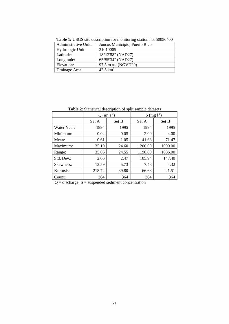
21

Table 1: USGS site description for monitoring station no. 50056400

Administrative Unit: Juncos Municipio, Puerto Rico

Hydrologic Unit: 21010005

Latitude: 18°12'58" (NAD27)

Longitude: 65°55'34" (NAD27)

Elevation: 97.5 m asl (NGVD29)

Drainage Area: 42.5 km2

Table 2: Statistical description of split sample datasets

Q (m3 s

-1) S (mg l

-1)

Set A Set B Set A Set B

Water Year: 1994 1995 1994 1995

Minimum: 0.04 0.05 2.00 4.00

Mean: 0.61 1.05 41.63 71.47

Maximum: 35.10 24.60 1200.00 1090.00

Range: 35.06 24.55 1198.00 1086.00

Std. Dev.: 2.06 2.47 105.94 147.40

Skewness: 13.59 5.73 7.48 4.32

Kurtosis: 218.72 39.80 66.68 21.51

Count: 364 364 364 364

Q = discharge; S = suspended sediment concentration

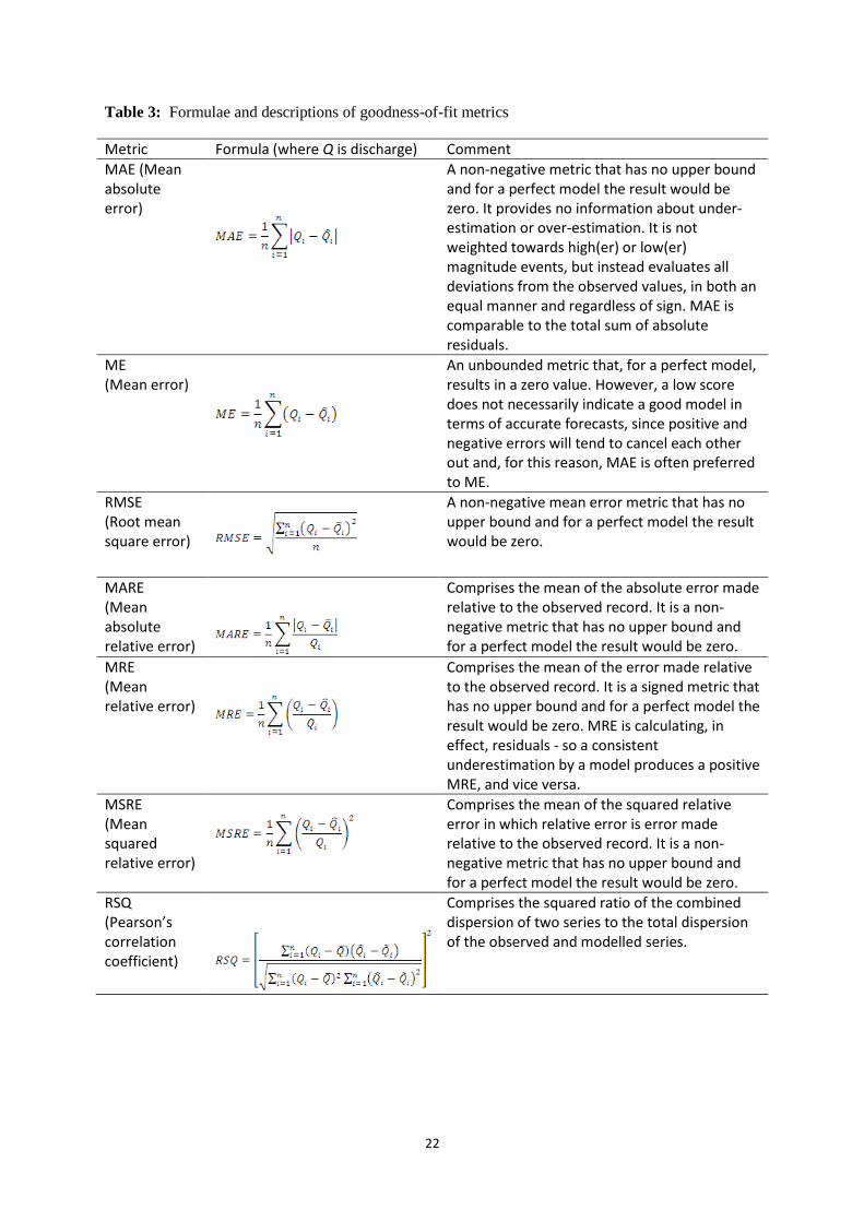
22

Table 3: Formulae and descriptions of goodness-of-fit metrics

Metric Formula (where Q is discharge) Comment

MAE (Mean absolute error)

A non-negative metric that has no upper bound and for a perfect model the result would be zero. It provides no information about under-estimation or over-estimation. It is not weighted towards high(er) or low(er) magnitude events, but instead evaluates all deviations from the observed values, in both an equal manner and regardless of sign. MAE is comparable to the total sum of absolute residuals.

ME (Mean error)

An unbounded metric that, for a perfect model, results in a zero value. However, a low score does not necessarily indicate a good model in terms of accurate forecasts, since positive and negative errors will tend to cancel each other out and, for this reason, MAE is often preferred to ME.

RMSE (Root mean square error)

A non-negative mean error metric that has no upper bound and for a perfect model the result would be zero.

MARE (Mean absolute relative error)

Comprises the mean of the absolute error made relative to the observed record. It is a non-negative metric that has no upper bound and for a perfect model the result would be zero.

MRE (Mean relative error)

Comprises the mean of the error made relative to the observed record. It is a signed metric that has no upper bound and for a perfect model the result would be zero. MRE is calculating, in effect, residuals - so a consistent underestimation by a model produces a positive MRE, and vice versa.

MSRE (Mean squared relative error)

Comprises the mean of the squared relative error in which relative error is error made relative to the observed record. It is a non-negative metric that has no upper bound and for a perfect model the result would be zero.

RSQ (Pearson’s correlation coefficient)

Comprises the squared ratio of the combined dispersion of two series to the total dispersion of the observed and modelled series.

23

Table 4: NF parameter settings and rule set for Equations 1-8

NFT-1 NFT-2

Number of MFs – 2

Type of MF – triangular

Triangular parameters:

a b c

MF1 -35.02 0.0714 35.03

MF2 0.0070 35.13 70.16

Rules:

If Q is MF1 then S1 is -226.4Q + 4.912

If Q is MF2 then S2 is -270.7Q + 10560

Number of MFs – 2

Type of MF – triangular

Triangular parameters:

a b c

MF1 -24.5 0.0135 24.64

MF2 0.1177 24.56 49.15

Rules:

If Q is MF1 then S1 is 29.79Q + 3.583

If Q is MF2 then S2 is -11.49Q + 1274

NFG-1 NFG-2

Number of MFs – 2

Type of MF – Gaussian

Gaussian parameters:

c

MF1 14.93 0.0324

MF2 14.95 35.05

Rules:

If Q is MF1 then S1 is 37.51Q – 169.9

If Q is MF2 then S2 is -49.34Q + 2775

Number of MFs – 2

Type of MF – Gaussian

Gaussian parameters:

c

MF1 10.47 0.0280

MF2 10.48 24.54

Rules:

If Q is MF1 then S1 is 100.6Q + 43.56

If Q is MF2 then S2 is 73.11Q – 776.3

24

Table 5: NN parameter settings for Equations 9-13

NNL-1 NNN-1 NNL-2 NNN-2

W1 (weight of hidden layer) 11.4319 -6.1670 7.8000 -5.0555

W2 (weight of output layer) 0.8359 -10.5612 0.6846 -23.1867

B1 (bias factor of hidden layer) -2.6970 0.0985 -2.0471 -1.3031

B2 (bias factor of output layer) -0.0410 1.3425 -0.0721 1.1041

Qmin (minimum observed Q) 0.0396 0.0396 0.0510 0.0510

Qmax (maximum observed Q) 35.1000 35.1000 24.6000 24.6000

Smin (minimum observed S) 2.0000 2.0000 4.0000 4.0000

Smax (maximum observed S) 1200.0000 1200.0000 1090.0000 1090.0000

25

Table 6: Numerical verification against earlier paper

* recalculated, using reported ‘total estimated sediment’

RMSE RSqr TE (%)

Model Kisi (2005) Abrahart et al. Kisi (2005) Abrahart et al. Kisi (2005)* Abrahart et al.

NFT-1 51.89 51.96 0.88 0.88 -1.82 -1.54 NNL-1 54.57 57.10 0.87 0.85 -1.99 2.93 PFT-1 58.38 58.30 0.85 0.85 -7.36 -7.58 SLR-1 74.41 74.12 0.84 0.84 -29.24 -29.07

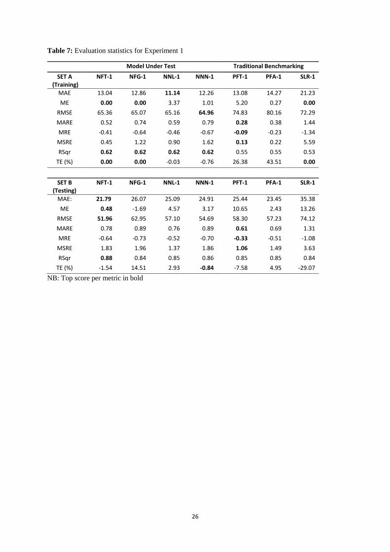
26

Table 7: Evaluation statistics for Experiment 1

Model Under Test Traditional Benchmarking

SET A (Training)

NFT-1 NFG-1 NNL-1 NNN-1 PFT-1 PFA-1 SLR-1

MAE 13.04 12.86 11.14 12.26 13.08 14.27 21.23

ME 0.00 0.00 3.37 1.01 5.20 0.27 0.00

RMSE 65.36 65.07 65.16 64.96 74.83 80.16 72.29

MARE 0.52 0.74 0.59 0.79 0.28 0.38 1.44

MRE -0.41 -0.64 -0.46 -0.67 -0.09 -0.23 -1.34

MSRE 0.45 1.22 0.90 1.62 0.13 0.22 5.59

RSqr 0.62 0.62 0.62 0.62 0.55 0.55 0.53

TE (%) 0.00 0.00 -0.03 -0.76 26.38 43.51 0.00

SET B (Testing)

NFT-1 NFG-1 NNL-1 NNN-1 PFT-1 PFA-1 SLR-1

MAE: 21.79 26.07 25.09 24.91 25.44 23.45 35.38

ME 0.48 -1.69 4.57 3.17 10.65 2.43 13.26

RMSE 51.96 62.95 57.10 54.69 58.30 57.23 74.12

MARE 0.78 0.89 0.76 0.89 0.61 0.69 1.31

MRE -0.64 -0.73 -0.52 -0.70 -0.33 -0.51 -1.08

MSRE 1.83 1.96 1.37 1.86 1.06 1.49 3.63

RSqr 0.88 0.84 0.85 0.86 0.85 0.85 0.84

TE (%) -1.54 14.51 2.93 -0.84 -7.58 4.95 -29.07

NB: Top score per metric in bold

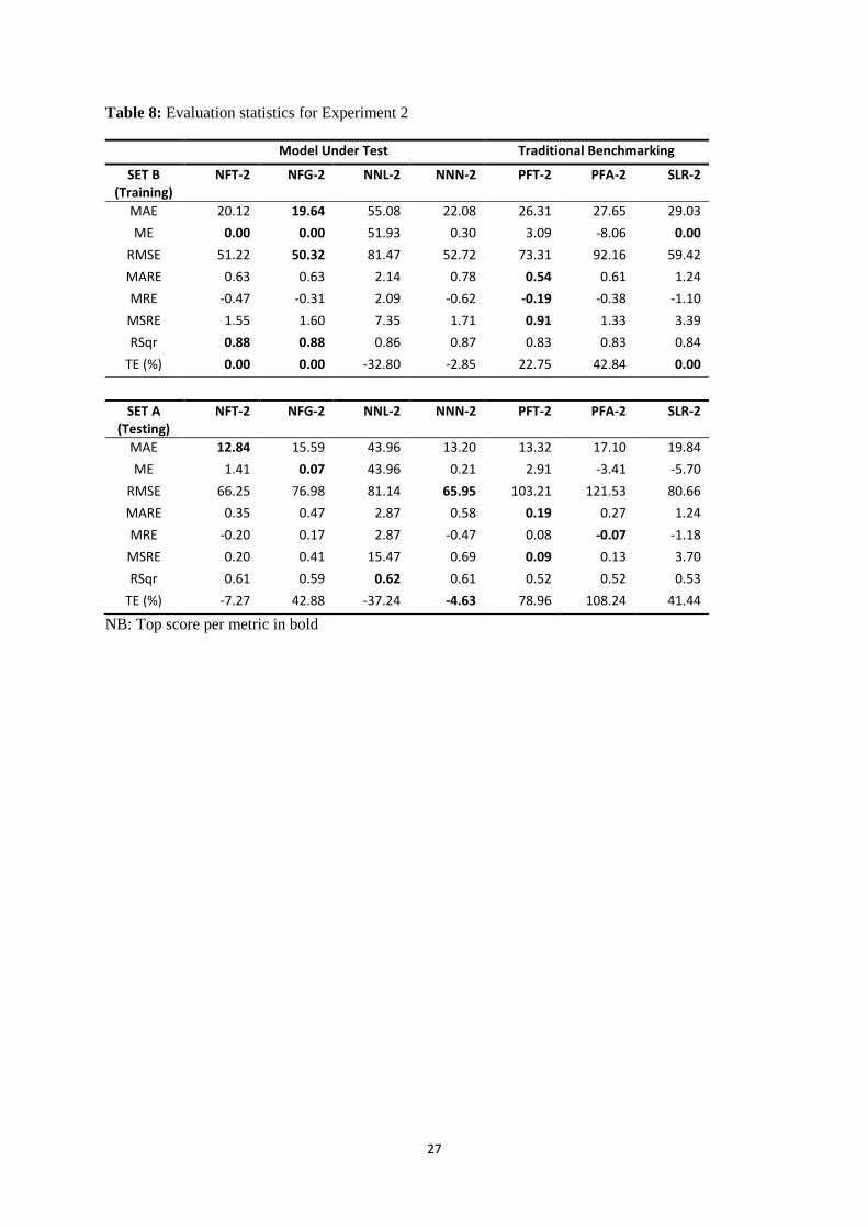
27

Table 8: Evaluation statistics for Experiment 2

Model Under Test Traditional Benchmarking

SET B (Training)

NFT-2 NFG-2 NNL-2 NNN-2 PFT-2 PFA-2 SLR-2

MAE 20.12 19.64 55.08 22.08 26.31 27.65 29.03

ME 0.00 0.00 51.93 0.30 3.09 -8.06 0.00

RMSE 51.22 50.32 81.47 52.72 73.31 92.16 59.42

MARE 0.63 0.63 2.14 0.78 0.54 0.61 1.24

MRE -0.47 -0.31 2.09 -0.62 -0.19 -0.38 -1.10

MSRE 1.55 1.60 7.35 1.71 0.91 1.33 3.39

RSqr 0.88 0.88 0.86 0.87 0.83 0.83 0.84

TE (%) 0.00 0.00 -32.80 -2.85 22.75 42.84 0.00

SET A (Testing)

NFT-2 NFG-2 NNL-2 NNN-2 PFT-2 PFA-2 SLR-2

MAE 12.84 15.59 43.96 13.20 13.32 17.10 19.84

ME 1.41 0.07 43.96 0.21 2.91 -3.41 -5.70

RMSE 66.25 76.98 81.14 65.95 103.21 121.53 80.66

MARE 0.35 0.47 2.87 0.58 0.19 0.27 1.24

MRE -0.20 0.17 2.87 -0.47 0.08 -0.07 -1.18

MSRE 0.20 0.41 15.47 0.69 0.09 0.13 3.70

RSqr 0.61 0.59 0.62 0.61 0.52 0.52 0.53

TE (%) -7.27 42.88 -37.24 -4.63 78.96 108.24 41.44

NB: Top score per metric in bold

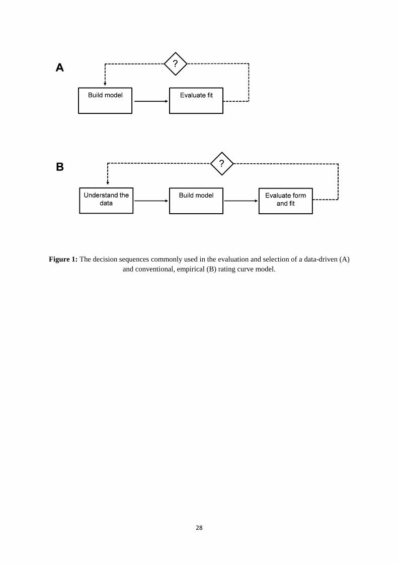
28

Figure 1: The decision sequences commonly used in the evaluation and selection of a data-driven (A)

and conventional, empirical (B) rating curve model.

29

Figure 2: The decision sequence underpinning DAMP, in which model selection is made on the basis

of a parallel evaluation of both 1) the form of the model and its fit to the data and 2) the hydrological

and physiographic context which underpins the understanding of the dataset to be modelled.

30

Figure 3: Location of two original gauging stations in Puerto Rico

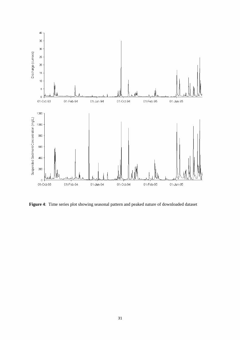
31

Figure 4: Time series plot showing seasonal pattern and peaked nature of downloaded dataset

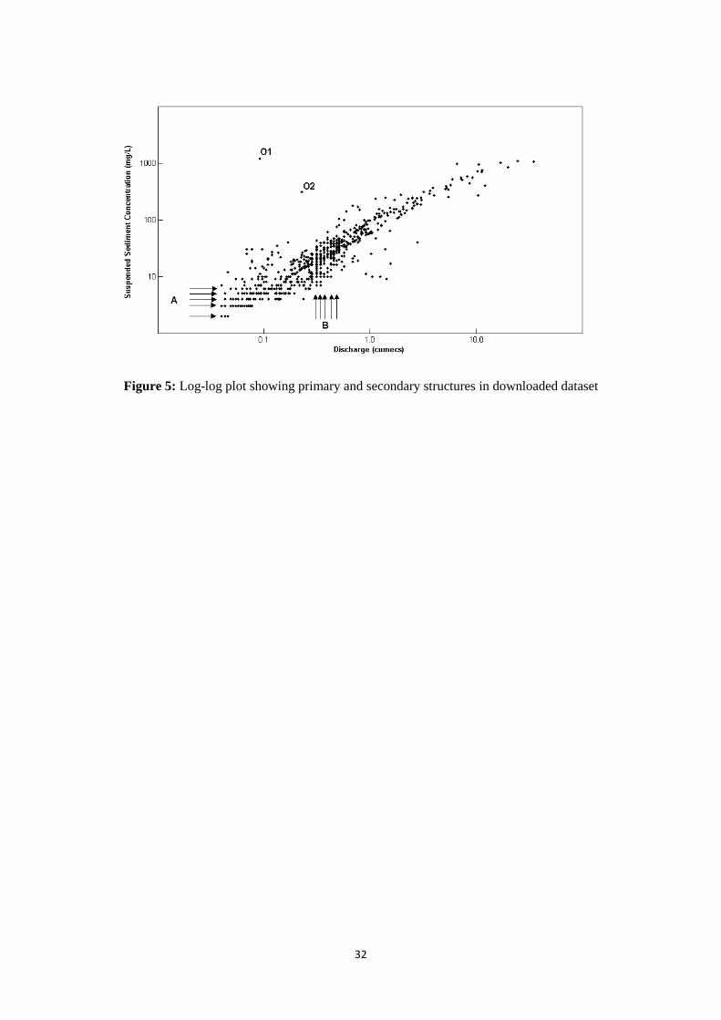
32

Figure 5: Log-log plot showing primary and secondary structures in downloaded dataset

33

Figure 6: NF architecture for one-input two-membership-function model

34

Figure 7: Triangular membership function: MF1 and MF2 for NFT-1

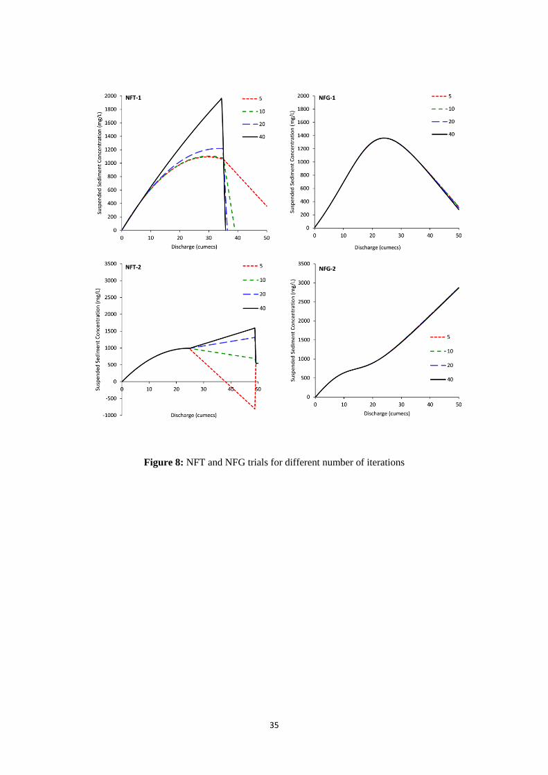
35

Figure 8: NFT and NFG trials for different number of iterations

36

Figure 9: NN architecture for a 1:1:1 model, containing non-linear intermediate hidden layer

and linear final output layer processing units

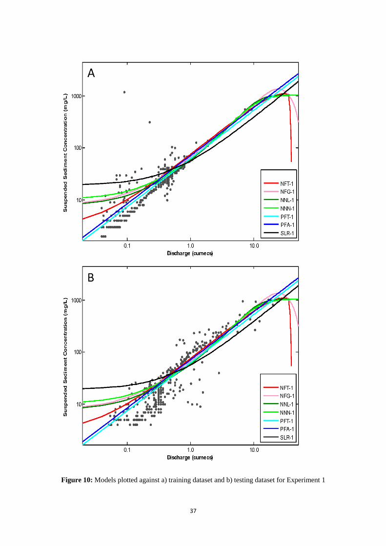
37

Figure 10: Models plotted against a) training dataset and b) testing dataset for Experiment 1

38

Figure 11: Models plotted against a) training dataset and b) testing dataset for Experiment 2