Embed Size (px)
Citation preview

Damage in Railway Crossings -
Numerical Models
Dissertation
zur Erlangung des akademischen Grades
Doktor der montanistischen Wissenschaften
an der Montanuniversität Leoben
eingereicht von
Martin Pletz
Institut für Mechanik
Montanuniversität Leoben
Leoben, 20. Juli 2012
ii
Acknowledgements
Danksagung
Für die Begutachtung dieser Arbeit und für die offizielle Betreuung möchte ich mich
herzlich bei Univ.-Prof. Thomas Antretter vom Institut für Mechanik bedanken.
Auch danke ich Dr. Werner Daves, dem Leiter der Rad/Schiene/Weichen Projekte,
für die Betreuung vor und während dieser Dissertation. Und die zahlreichen
Diskussionen, aus denen diese Arbeit hervorgegangen ist.
Die vorgestellte Arbeit wurde in einem Forschungsprojekt mit der VAE GmbH in
Zeltweg durchgeführt. Sollte der eine oder andere Teil dieser Arbeit gut geworden
sein, so hat das ganz entscheidend mit der Unterstützung und den Diskussionen mit
der VAE, allem voran DI Heinz Ossberger, zu tun. Dafür herzlichen Dank.
Außerdem danke ich Univ.-Prof. Robert Danzer vom Institut für Struktur- und
Funktionskeramik (ISFK) dafür dass ich während meiner Dissertation am ISFK sitzen
durfte und er mir einiges übers Präsentieren und Schreiben beigebracht hat. Herzlich
danke ich meinen Kollegen am ISFK, besonders Dr. Raul Bermejo und Dr. Marco
Deluca.
Zum Schluss möchte ich mich bei meinen Eltern Bernhard und Christa und meinen
Brüdern Jakob, Lukas und Tobias bedanken. Für ihre Unterstützung bei dieser
Dissertation und auch sonst.
Der österreichischen Bundesregierung (insbesondere dem Bundesministerium für
Verkehr, Innovation und Technologie und dem Bundesministerium für Wirtschaft,
Familie und Jugend) sowie dem Land Steiermark, vertreten durch die
Österreichische Forschungsförderungsgesellschaft mbH und die Steirische
Wirtschaftsförderungsgesellschaft mbH, wird für die finanzielle Unterstützung der
Forschungsarbeiten im Rahmen des von der Materials Center Leoben Forschung
GmbH abgewickelten K2 Zentrums für „Materials, Processing und Product
Engineering“ im Rahmen des Österreichischen COMET Kompetenzzentren
Programms herzlich gedankt.
iii
Abstract
Damage in rails and turnouts is an important issue as it is one of the main causes for
maintenance such as reprofiling (grinding) and replacing of rails. In the contact areas
between rail and wheel, very high loads are produced that cause this damage in the
form of wear and development of surface cracks. In the crossing panel of turnouts,
the wheel has to change from one rail to another, causing a vertical impact. As the
wheel has to roll on different rolling radii during this change, slip is produced. The
impact thus leads to high contact pressures and high slip. Important parameters of
the impact are the train speed, the wheel profile, the axle load and the crossing’s
support. In this thesis, dynamic and quasi-static finite element models for the passing
over the crossing have been developed. Three models are used for describing the
damage arising in crossings: A global dynamic model that calculates the run of a
wheel through a three- metre crossing, a dynamic model that calculates the repeated
impact of the wheel on the crossing nose and a quasi-static two-dimensional crack
model. Loads have been transferred between those models, which shows that there
are three important mechanisms for damage in crossings: a) The dynamics of the
impact, determined mainly by crossing and wheel geometry, train speed and crossing
support, b) the plastic adaption of the crossing to the wheel profile and c) the build-up
of residual stresses near the crossing’s surface. The plastic adaption and the residual
stresses both reduce the loading of a crack and strongly depend on the plastic
behaviour of the crossing material. Understanding these mechanisms that cause the
loading of crossings allow for the optimization of crossings in terms of their material,
support and geometry.
iv
Zusammenfassung
Schädigung in Schienen und Weichen ist einer der Hauptverursacher für
Wartungsarbeiten wie Schienenschleifen und Austausch von Schienen im Gleis. In
den Kontaktflächen zwischen Rad und Schiene wirken hohe Lasten, die zu einer
Schädigung in Form von Verschleiß und Rissbildung führen. Im Bereich der
Herzstücke von Weichen wechselt das Rad seinen Lauf von einer Schiene auf eine
andere. Dabei muss es sich aus geometrischen Gründen und abhängig von der
Bauart der Weiche nach unten und oben bewegen, was in einem vertikalen Stoß
resultiert. Da das Rad eine konische Lauffläche besitzt und sich die
Kontaktpositionen am Rad während diesem Überlauf ändern, kommt es dabei auch
zu Schlupf. Dieser Stoß führt somit zu hohen Kontaktdrücken und hohem Schlupf,
die durch Parameter wie die Zuggeschwindigkeit, das Radprofil, die Achslast und die
Lagerung der Weiche bestimmt werden. In dieser Arbeit wurden dynamische und
quasistatische finite Elemente Modelle für den Herzstücküberlauf entwickelt. Drei
Modelle berechnen die Schädigung in Herzstücken: Ein globales dynamisches
Modell mit einem Radlauf über drei Meter des Herzstücks, ein dynamisches Modell
für den wiederholten Stoß des Rads auf der Herzspitze und ein quaststatisches
zweidimensionales Modell mit einem Oberflächenriss. Die Belastungen werden
zwischen den einzelnen Modellen übertragen. Es zeigt sich, dass es drei wichtige
Mechanismen gibt, die für Schädigung in Herzstücken verantwortlich sind: a) Der
dynamische Stoß des Rads beim Aufsetzen, bei dem die Geometrie von Rad und
Herzstück, Zuggeschwindigkeit und Lagerung des Herzstücks eine wichtige Rolle
spielen, b) die geometrische Anpassung der Herzspitze (durch plastische
Verformung) an das Radprofil und c) der Aufbau von Eigenspannungen nahe der
Herzstückoberfläche. Die plastische Anpassung des Herzstücks und die
Eigenspannungen reduzieren im Allgemeinen die Belastung eines Risses im
Kontaktbereich, wobei das plastische Materialverhalten des Herzstücks dabei eine
entscheidende Rolle spielt. Das Verständnis dieser Belastungsmechanismen erlaubt
Vorhersagen über den Einfluss des Materials, der Lagerung und der Geometrie von
Herzstücken. Damit können in weiterer Folge Herzstücke optimiert werden.
v
Compilation of thesis
This thesis consists of an extended summary and the following appended papers
Paper A Pletz, M., Daves, W., and Ossberger, H., A Wheel Set / Crossing Model
Regarding Impact, Sliding and Deformation- Explicit Finite Element
Approach. Under Revision- Wear.
Paper B Pletz, M., Daves, W., and Ossberger, H., A Wheel Passing a Crossing
Nose- Dynamic Analysis under High Axle Loads using Finite Element
Modelling. Accepted for publication in Proceedings of the Institution of
Mechanical Engineers, Part F: Journal of Rail and Rapid Transit, 2012.
Paper C Pletz, M., Daves, W., Eck, S., and Ossberger, H., The Plastic Adaption
of Railway Crossings due to Dynamic Contact Loading - Explicit Finite
Element Study. To be submitted.
Paper D Pletz, M., Daves, W., Yau, W., and Ossberger, H., Prediction of Rolling
Contact Fatigue in Crossings- Multiscale FE Model, in Proceeding at
the 8th International Conference on Contact Mechanics and Wear of
Rail/Wheel Systems, Chengdu, China, 2012.
vi
Related papers by the author
Paper E Pletz, M., Daves, W., Fischer, F.D. and Ossberger, H., A Dynamical
Wheel Set: Crossing Model Regarding Impact, Sliding and
Deformation, in Proceeding at the 8th International Conference on
Contact Mechanics and Wear of Rail/Wheel Systems, Florence, Italy,
pp 801-809, 2009.
Paper F Pletz, M., Daves, W., and Ossberger, H., Dynamic Finite Element
Model of a Wheel Passing a Crossing Nose. Proceedings of the tenth
international conference on computational structures technology,
Valencia, Spain, 2010.
Paper G Pletz, M., Daves, W., and Ossberger, H., A Wheel Passing a Frog
Nose- Dynamic Finite Element Investigation of High Axle Loads,
Proceedings of the International Heavy Haul Association Conference,
Calgary, Canada, 2011, on-line.
Paper H Pletz, M., Daves, W., Yau, W., and Ossberger, H., Multi-Scale finite
element model to describe wear and rolling contact fatigue in the wheel
– rail test rig, in Proceeding at the 8th International Conference on
Contact Mechanics and Wear of Rail/Wheel Systems, Chengdu, China,
2012.
Paper I Pletz, M., Daves, W., and Ossberger, H., Understanding the Loading of
Railway Crossings, Railway Gazette, August Issue, 2012.
vii
Contribution to papers
Paper A (Extended version of paper E and F), paper B (extended version of
paper G) and paper C
Responsible for the development of the method.
Carried out the numerical simulations.
Wrote most parts of the paper.
Paper D
Responsible for the development of the crossing model, the impact model and
the methodology for combining the models on different length scales.
Carried out the numerical simulations for the crossing and the impact model
(the crack model simulations were carried out by Weiping Yao).
Wrote most parts of the paper.
Paper H
Responsible for the development of the three-dimensional test-rig model and
the methodology for combining the models on different length scales.
Carried out the numerical simulations for 3D test-rig model (the crack model
simulations were carried out by W. Yao and the roughness model calculations
by W.K. Kubin).
Wrote most parts of the paper.
Paper I
Responsible for the development of the method.
Carried out the numerical simulations.
Wrote most parts of the paper.
The extended summary of this thesis is nearly identical to Paper I. The support of
Railway Gazette is gratefully acknowledged.
viii
Affidavit
I declare in lieu of oath, that I wrote this thesis and performed the associated research myself, using only literature cited in this volume. Leoben, July 2012
Martin Pletz

ix
Contents
1. Introduction 1
2. The FE Model 3
3. Mechanisms of Loading 5
3.1 Vertical Position of Wheel- Impact 7
3.2 Angular Velocity of Wheel- Slip 11
3.3 Putting it all together 15
4. The role of plastic material behaviour 16
5. Studying the loading of a surface crack 19
6. Conclusions 20
Paper A 24
Paper B 48
Paper C 65
Paper D 90

Extended Summary
1 Introduction
Turnouts are an important part of the track structure as they allow trains to switch
from one track to the other. They are also a weak spot in the track structure as they
cause an impact of the wheel in the horizontal (at the switch panel) or in the vertical
direction (at the crossing nose). Issues such as wear and rolling contact fatigue
(RCF) are thus very important for turnouts. In Figure 1, a typical rigid crossing is
shown. It consists of two wing rails and a crossing nose. Moving from the front to the
back in Figure 1 (facing move), the wheel runs initially on one wing rail and then
impacts onto the crossing nose. In the opposite direction, the wheel impacts onto the
wing rail. In the track, more damage is observed on the crossing nose than on the
wing rail and thus the facing move is the more critical case for the evolution of
damage. The model in this work thus only simulates the facing move.
Figure 1: A picture of a rigid crossing. The wing rails and the crossing nose are highlighted.
One aim of the turnout producers is to minimize or, in the ideal case, totally avoid
these increased loads to extend the lifetime and the maintenance intervals of
turnouts. Crossings with movable crossing noses (in contrast to the rigid crossings)
can nearly totally avoid the vertical impact of the wheel, but are due to their high
costs only used in special applications such as high speed tracks or heavy haul lines.
Understanding the factors that influence the loading of these crossings and as a
consequence their damage provides a basis for the optimization of the crossing
geometry, crossing material and properties of the elastic support. In this work, a finite
element (FE) model is presented which simulates a wheel running over a crossing.
2
Parameters such as the train velocity, the wheel profile, the crossing's support and
the axle load are varied to see the influences on the arising loads. With simplified
analytical models, the origin of contact pressures and slip is explained.
Most commonly calculations for turnouts are done with multi body system (MBS)
simulation tools, which model the whole train and track structure using point masses,
springs and dashpots. The whole train and long parts of the track can be modelled.
Simplified contact models provide the interaction of the wheels and crossing parts.
Inelastic material behaviour cannot be used directly. Such calculations can e.g. be
found in [1].
Focusing on the influences of load parameters on the material response, a simplified
FE crossing model was developed by the authors. It is a fully dynamic model based
on the method of finite elements, which calculates just one wheel running over the
crossing. Therefore reasonable but simplified assumptions have to be made about
the lateral wheel position and influence of the wheel set during the crossing process.
Within the group of involved engineers and scientists it has been shown that the
understanding and prediction of the development of surface damage in rails such as
wear, crack initiation and growth (commonly referred to as rolling contact fatigue-
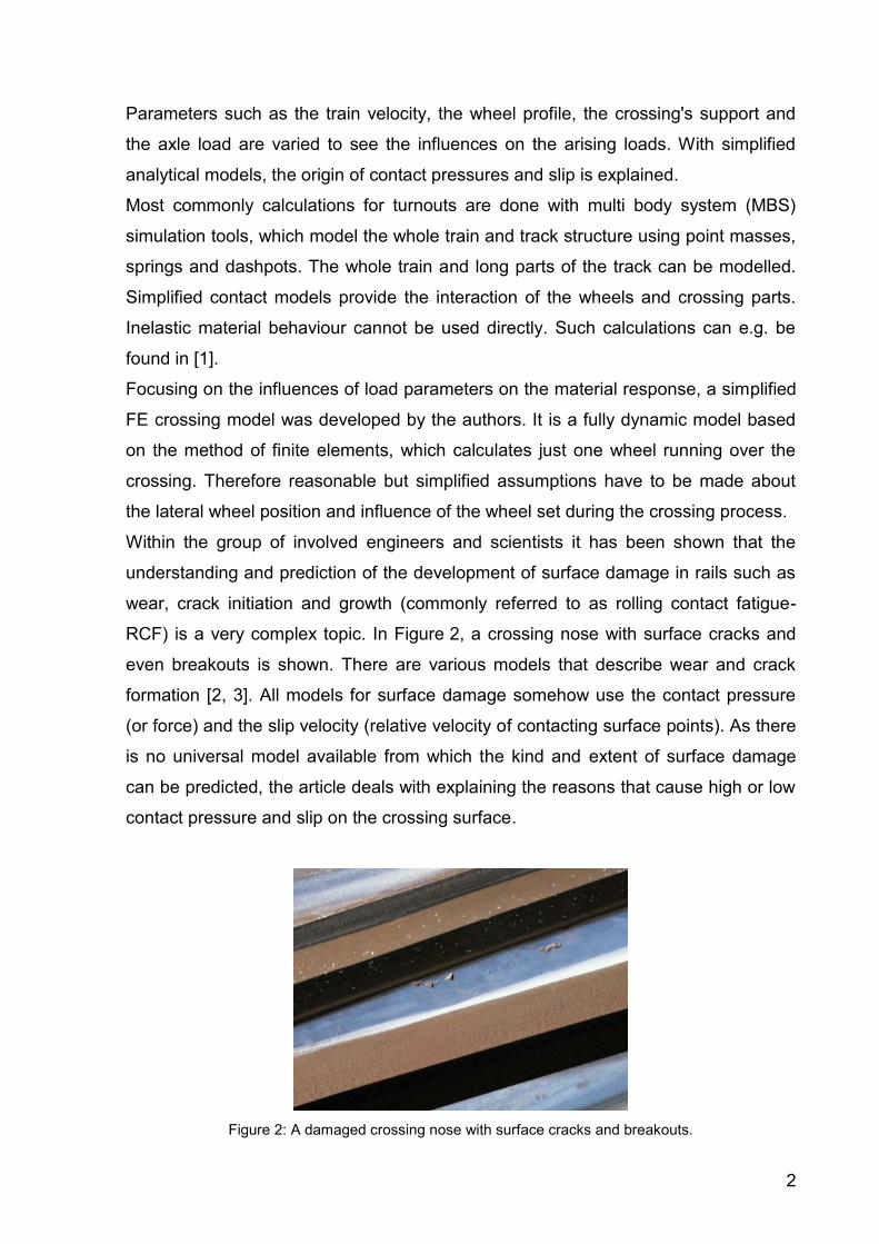
RCF) is a very complex topic. In Figure 2, a crossing nose with surface cracks and
even breakouts is shown. There are various models that describe wear and crack
formation [2, 3]. All models for surface damage somehow use the contact pressure
(or force) and the slip velocity (relative velocity of contacting surface points). As there
is no universal model available from which the kind and extent of surface damage
can be predicted, the article deals with explaining the reasons that cause high or low
contact pressure and slip on the crossing surface.
Figure 2: A damaged crossing nose with surface cracks and breakouts.
3
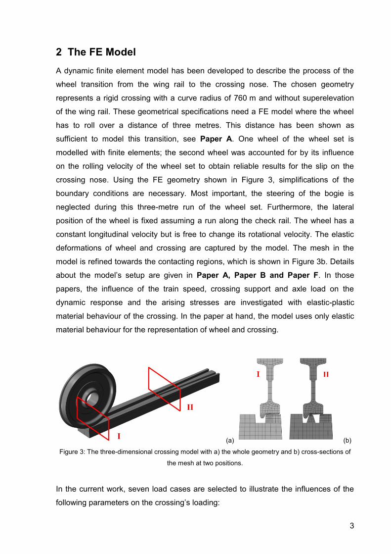
2 The FE Model
A dynamic finite element model has been developed to describe the process of the
wheel transition from the wing rail to the crossing nose. The chosen geometry
represents a rigid crossing with a curve radius of 760 m and without superelevation
of the wing rail. These geometrical specifications need a FE model where the wheel
has to roll over a distance of three metres. This distance has been shown as
sufficient to model this transition, see Paper A. One wheel of the wheel set is
modelled with finite elements; the second wheel was accounted for by its influence
on the rolling velocity of the wheel set to obtain reliable results for the slip on the
crossing nose. Using the FE geometry shown in Figure 3, simplifications of the
boundary conditions are necessary. Most important, the steering of the bogie is
neglected during this three-metre run of the wheel set. Furthermore, the lateral
position of the wheel is fixed assuming a run along the check rail. The wheel has a
constant longitudinal velocity but is free to change its rotational velocity. The elastic
deformations of wheel and crossing are captured by the model. The mesh in the
model is refined towards the contacting regions, which is shown in Figure 3b. Details
about the model’s setup are given in Paper A, Paper B and Paper F. In those
papers, the influence of the train speed, crossing support and axle load on the
dynamic response and the arising stresses are investigated with elastic-plastic
material behaviour of the crossing. In the paper at hand, the model uses only elastic
material behaviour for the representation of wheel and crossing.
(a) (b)
Figure 3: The three-dimensional crossing model with a) the whole geometry and b) cross-sections of
the mesh at two positions.
In the current work, seven load cases are selected to illustrate the influences of the
following parameters on the crossing’s loading:
4
Wheel profile
Train speed
Crossing support
Axle load
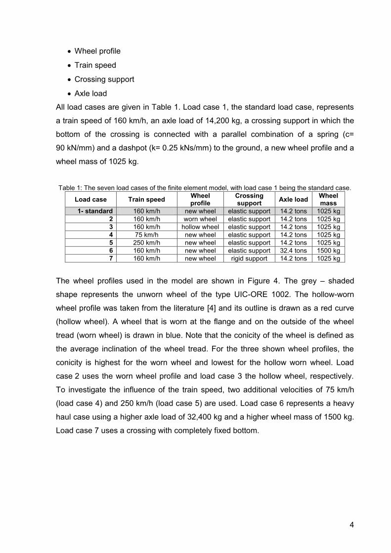
All load cases are given in Table 1. Load case 1, the standard load case, represents
a train speed of 160 km/h, an axle load of 14,200 kg, a crossing support in which the
bottom of the crossing is connected with a parallel combination of a spring (c=
90 kN/mm) and a dashpot (k= 0.25 kNs/mm) to the ground, a new wheel profile and a
wheel mass of 1025 kg.
Table 1: The seven load cases of the finite element model, with load case 1 being the standard case.
Load case Train speed Wheel profile
Crossing support
Axle load Wheel mass
1- standard 160 km/h new wheel elastic support 14.2 tons 1025 kg
2 160 km/h worn wheel elastic support 14.2 tons 1025 kg
3 160 km/h hollow wheel elastic support 14.2 tons 1025 kg
4 75 km/h new wheel elastic support 14.2 tons 1025 kg
5 250 km/h new wheel elastic support 14.2 tons 1025 kg
6 160 km/h new wheel elastic support 32.4 tons 1500 kg
7 160 km/h new wheel rigid support 14.2 tons 1025 kg
The wheel profiles used in the model are shown in Figure 4. The grey – shaded
shape represents the unworn wheel of the type UIC-ORE 1002. The hollow-worn
wheel profile was taken from the literature [4] and its outline is drawn as a red curve
(hollow wheel). A wheel that is worn at the flange and on the outside of the wheel
tread (worn wheel) is drawn in blue. Note that the conicity of the wheel is defined as
the average inclination of the wheel tread. For the three shown wheel profiles, the
conicity is highest for the worn wheel and lowest for the hollow worn wheel. Load
case 2 uses the worn wheel profile and load case 3 the hollow wheel, respectively.
To investigate the influence of the train speed, two additional velocities of 75 km/h
(load case 4) and 250 km/h (load case 5) are used. Load case 6 represents a heavy
haul case using a higher axle load of 32,400 kg and a higher wheel mass of 1500 kg.
Load case 7 uses a crossing with completely fixed bottom.

5
Figure 4: The three used wheel profiles. The new wheel is shown in grey, the hollow-worn wheel in red
(case: hollow wheel) and the wheel with wear on the flange and on the outside of the tread is shown in
blue (case: worn wheel).
3 Mechanisms of Loading
During the rolling of a wheel over a crossing, the wheel changes its run from the wing
rail to the crossing nose. To enable a smooth transition of the wheel, the crossings
need to have a certain geometry where the wing rail deviates from the general track
direction, henceforth denoted as “deviating wing rail”. Because of that geometry, the
contact point of the wheel continuously changes its lateral position on the wheel
tread. As some of the mechanisms of the crossing's loading can be explained by
these changes and the corresponding running wheel radius, this is described in more
detail. In Figure 5, the crossing is cut at three selected longitudinal positions and the
contact geometries in these cross-sections is shown. It can be seen that initially
(before reaching the deviating part of the wing rail) the wheel contacts the wing rail in
the middle of its tread. As the wheel approaches the crossing, this contact position
moves away from the flange. The first contact of the wheel with the crossing nose is
close to the wheel’s flange. After the impact on the crossing, the lateral contact point
on the wheel moves back to the middle of the wheel tread.
Figure 5: Three cross-sections of the wheel-crossing contact before, during and after the impact of the
wheel onto the crossing nose. Note the different contact positions on the wheel tread.
6
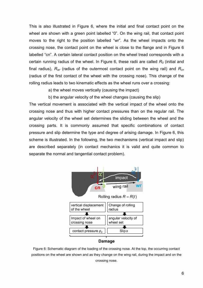
This is also illustrated in Figure 6, where the initial and final contact point on the
wheel are shown with a green point labelled “0”. On the wing rail, that contact point
moves to the right to the position labelled “wr”. As the wheel impacts onto the
crossing nose, the contact point on the wheel is close to the flange and in Figure 6
labelled “cn”. A certain lateral contact position on the wheel tread corresponds with a
certain running radius of the wheel. In Figure 6, these radii are called R0 (initial and
final radius), Rwr (radius of the outermost contact point on the wing rail) and Rcn
(radius of the first contact of the wheel with the crossing nose). This change of the
rolling radius leads to two kinematic effects as the wheel runs over a crossing:
a) the wheel moves vertically (causing the impact)
b) the angular velocity of the wheel changes (causing the slip)
The vertical movement is associated with the vertical impact of the wheel onto the
crossing nose and thus with higher contact pressures than on the regular rail. The
angular velocity of the wheel set determines the sliding between the wheel and the
crossing parts. It is commonly assumed that specific combinations of contact
pressure and slip determine the type and degree of arising damage. In Figure 6, this
scheme is illustrated. In the following, the two mechanisms (vertical impact and slip)
are described separately (in contact mechanics it is valid and quite common to
separate the normal and tangential contact problem).
Figure 6: Schematic diagram of the loading of the crossing nose. At the top, the occurring contact
positions on the wheel are shown and as they change on the wing rail, during the impact and on the
crossing nose.

7
3.1 Vertical Movement of the Wheel – Impact
The impact of the wheel on the crossing nose is caused by the change of the moving
direction of the wheel. Since the wheel is moving downward during its run on the
wing rail (e.g. by a distance of 3 mm for a new wheel), it has to climb up again to the
initial level on the crossing nose. In Figure 7a, this movement of the wheel centre is
shown for the standard load case. The grey line gives the vertical displacement of the
wheel centre, the green line the displacement of the crossing and the black line the
relative displacement of wheel and crossing. Below the diagram, a picture of a
crossing is shown that corresponds to the wheel positions.
In the beginning (wheel position of 0 – 0.2 metres) the wheel stays at about the same
level. As the wing rail starts to deviate at a wheel position of 0.2 m, the wheel centre
starts to move downwards. It continues its downward movement up to a position of
1.7 m, where it impacts onto the crossing nose. There, it starts to move upwards
again until it reaches the same level it had in the beginning. At the impact, there is an
angle (impact angle) between the relative wheel movement before and after the
impact. For the shown load case, this angle is 0.35°. The crossing is pressed
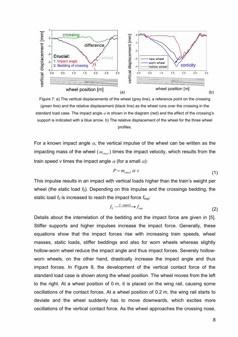
downwards at the impact thereby reducing the impact forces. In Figure 7b, the wheel
movements for the different wheel profiles are shown. It can be seen that the worn
wheel drops by nearly 4 mm and has with a value of 0.66° a higher than the
calculation with the new wheel. The hollow worn wheel has nearly no conicity of the
wheel tread and thus does not lower its vertical position on the wing rail during its run
towards the crossing nose. At a wheel position of 1.6 m, however, it suddenly drops
from the wing rail on the crossing nose accompanied by a higher impact angleof
0.86° This shows that there is a general tendency that decreasing wheel conicities
lower the impact angle but this is valid only to a certain extent. The impact angle is
mainly determined by the contact geometry. The other parameters (axle load, train
speed, crossing support) have nearly no influence on it.
8
(a) (b)
Figure 7: a) The vertical displacements of the wheel (grey line), a reference point on the crossing
(green line) and the relative displacement (black line) as the wheel runs over the crossing in the
standard load case. The impact angle is shown in the diagram (red) and the effect of the crossing’s
support is indicated with a blue arrow. b) The relative displacement of the wheel for the three wheel
profiles.
For a known impact angle , the vertical impulse of the wheel can be written as the
impacting mass of the wheel (wheelm ) times the impact velocity, which results from the
train speed v times the impact angle (for a small ):
wheelP m v (1)
This impulse results in an impact with vertical loads higher than the train’s weight per
wheel (the static load f0). Depending on this impulse and the crossings bedding, the
static load f0 is increased to reach the impact force fimp:
, support
0
P
impf f (2)
Details about the interrelation of the bedding and the impact force are given in [5].
Stiffer supports and higher impulses increase the impact force. Generally, these
equations show that the impact forces rise with increasing train speeds, wheel
masses, static loads, stiffer beddings and also for worn wheels whereas slightly
hollow-worn wheel reduce the impact angle and thus impact forces. Severely hollow-
worn wheels, on the other hand, drastically increase the impact angle and thus
impact forces. In Figure 8, the development of the vertical contact force of the
standard load case is shown along the wheel position. The wheel moves from the left
to the right. At a wheel position of 0 m, it is placed on the wing rail, causing some
oscillations of the contact forces. At a wheel position of 0.2 m, the wing rail starts to
deviate and the wheel suddenly has to move downwards, which excites more
oscillations of the vertical contact force. As the wheel approaches the crossing nose,

9
the amplitudes of these oscillations decrease due to dashpots connected to wheel
and the crossing. During the impact of the wheel on the crossing nose, the contact
force is significantly higher than the static load. During the further run of the wheel on
the crossing nose some more oscillations of the contact force occur, but due to the
broadening of the crossing nose they produce less contact stresses and are less
relevant as the first impact. The effect of the dynamic contact force fimp on arising
stresses during this first impact is strongly dependent on the position of impact ximp.
Both values are shown in Figure 8.
Figure 8: The vertical contact forces between the wheel and the crossing for the standard load case.
The dynamic contact force during the impact fimp (red) reaches a value of 147 kN at a wheel position of
impact ximp of 1.81 m.
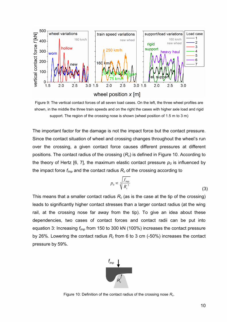
In Figure 9, the vertical contact forces for all 7 load cases are shown for wheel
positions from 1.5 to 3 metres, where the impact occurs. In the left diagram, the three
wheel profiles are compared. The earlier impact of the worn wheel (load case 2) can
be seen as well as the later impact of the hollow wheel (load case 3), causing
extremely high contact forces of 500 kN. The middle diagram in Figure 9 shows the
results for the three train speeds are shown. The impact position ximp is the same for
the three cases, but the contact forces of the impact increase with increasing train
speed v. On the right, the standard load case is compared with load case 6 (heavy
haul) and load case 7 (rigid support). For the heavy haul case, the level of the vertical
contact force is generally higher and thus high contact forces arise. For rigid support
of the crossing, the amplitudes of the oscillations are increased, causing high contact
forces. It can be seen that a stiffer support has a similar effect as higher train speeds.
10
Figure 9: The vertical contact forces of all seven load cases. On the left, the three wheel profiles are
shown, in the middle the three train speeds and on the right the cases with higher axle load and rigid
support. The region of the crossing nose is shown (wheel position of 1.5 m to 3 m)
The important factor for the damage is not the impact force but the contact pressure.
Since the contact situation of wheel and crossing changes throughout the wheel’s run
over the crossing, a given contact force causes different pressures at different
positions. The contact radius of the crossing (Rc) is defined in Figure 10. According to
the theory of Hertz [6, 7], the maximum elastic contact pressure p0 is influenced by
the impact force fimp and the contact radius Rc of the crossing according to
30 2
imp
c
fp
R
(3)
This means that a smaller contact radius Rc (as is the case at the tip of the crossing)
leads to significantly higher contact stresses than a larger contact radius (at the wing
rail, at the crossing nose far away from the tip). To give an idea about these
dependencies, two cases of contact forces and contact radii can be put into
equation 3: Increasing fimp from 150 to 300 kN (100%) increases the contact pressure
by 26%. Lowering the contact radius Rc from 6 to 3 cm (-50%) increases the contact
pressure by 59%.
Figure 10: Definition of the contact radius of the crossing nose Rc.
11
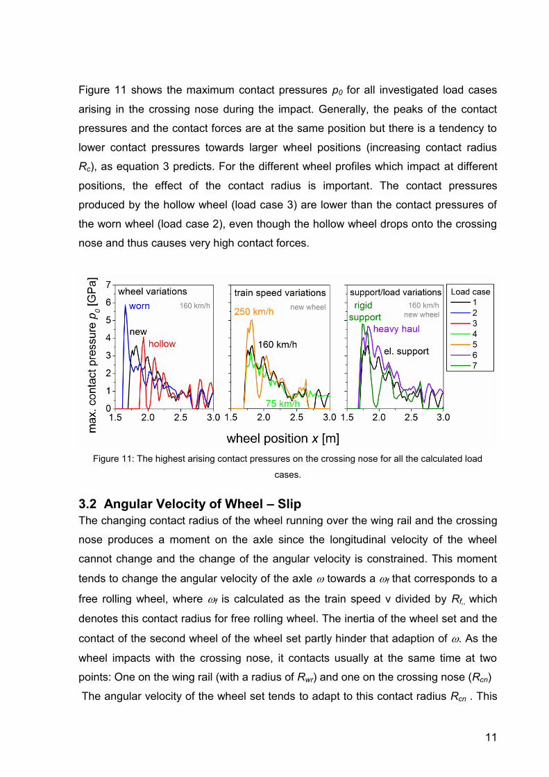
Figure 11 shows the maximum contact pressures p0 for all investigated load cases
arising in the crossing nose during the impact. Generally, the peaks of the contact
pressures and the contact forces are at the same position but there is a tendency to
lower contact pressures towards larger wheel positions (increasing contact radius
Rc), as equation 3 predicts. For the different wheel profiles which impact at different
positions, the effect of the contact radius is important. The contact pressures
produced by the hollow wheel (load case 3) are lower than the contact pressures of
the worn wheel (load case 2), even though the hollow wheel drops onto the crossing
nose and thus causes very high contact forces.
Figure 11: The highest arising contact pressures on the crossing nose for all the calculated load
cases.
3.2 Angular Velocity of Wheel – Slip
The changing contact radius of the wheel running over the wing rail and the crossing
nose produces a moment on the axle since the longitudinal velocity of the wheel
cannot change and the change of the angular velocity is constrained. This moment
tends to change the angular velocity of the axle towards a f that corresponds to a
free rolling wheel, where f is calculated as the train speed v divided by Rf,, which
denotes this contact radius for free rolling wheel. The inertia of the wheel set and the
contact of the second wheel of the wheel set partly hinder that adaption of . As the
wheel impacts with the crossing nose, it contacts usually at the same time at two
points: One on the wing rail (with a radius of Rwr) and one on the crossing nose (Rcn)
The angular velocity of the wheel set tends to adapt to this contact radius Rcn . This
12
process is partly hindered by the second wheel of the axle, which runs on the regular
rail. Any misfit between the angular velocity and the wheel radius Rf causes slip. As
long as the wheel is not driven or brakes, this misfit is the main cause of slip when
the wheel changes from the wing rail to the crossing nose. As the radius of the wheel
at the point contacting with the wing rail Rwr is smaller than the radius at the point
contacting with the crossing nose Rcn, the angular velocity is increased before and
decreased during the impact of the wheel onto the crossing nose.
Before the wheel impacts with the crossing nose the wheel adapts and increases its
angular velocity due to its decreasing contact radius on the deviating wing rail but
depending on the time available and its rotational inertia, the adaption is not always
complete. The more complete this adaption works out the higher is the resulting slip
during the impact.
As a maximum value of the slip during impact, it can be assumed that the angular
velocity of the axle fully adapts to Rwr and then it adapts to the radius Rcn on the
crossing nose. Using the definition of Carter for the slip s [8], in which the velocities
are expressed by the rolling radii, the maximum possible slip smax can be written as
max
2 cn wr
cn wr
R Rs
R R
(4)
This maximum possible slip smax depends on the wheel profile, too. Less conicity
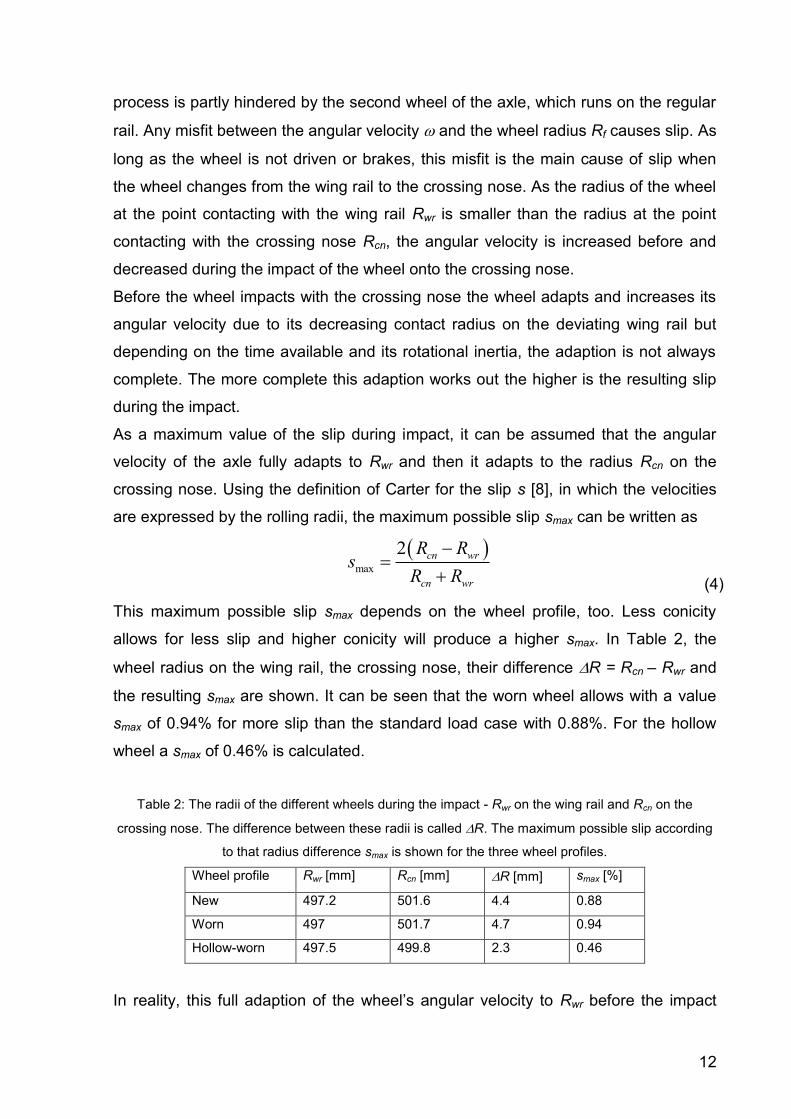
allows for less slip and higher conicity will produce a higher smax. In Table 2, the
wheel radius on the wing rail, the crossing nose, their difference R = Rcn – Rwr and
the resulting smax are shown. It can be seen that the worn wheel allows with a value
smax of 0.94% for more slip than the standard load case with 0.88%. For the hollow
wheel a smax of 0.46% is calculated.
Table 2: The radii of the different wheels during the impact - Rwr on the wing rail and Rcn on the
crossing nose. The difference between these radii is called R. The maximum possible slip according
to that radius difference smax is shown for the three wheel profiles.
Wheel profile Rwr [mm] Rcn [mm] R [mm] smax [%]
New 497.2 501.6 4.4 0.88
Worn 497 501.7 4.7 0.94
Hollow-worn 497.5 499.8 2.3 0.46
In reality, this full adaption of the wheel’s angular velocity to Rwr before the impact
13
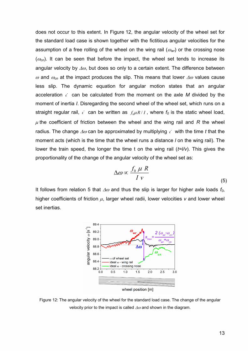
does not occur to this extent. In Figure 12, the angular velocity of the wheel set for
the standard load case is shown together with the fictitious angular velocities for the
assumption of a free rolling of the wheel on the wing rail (wr) or the crossing nose
(cn). It can be seen that before the impact, the wheel set tends to increase its
angular velocity by , but does so only to a certain extent. The difference between
and cn at the impact produces the slip. This means that lower values cause
less slip. The dynamic equation for angular motion states that an angular
acceleration can be calculated from the moment on the axle M divided by the
moment of inertia I. Disregarding the second wheel of the wheel set, which runs on a
straight regular rail, can be written as 0 /f R I , where f0 is the static wheel load,
the coefficient of friction between the wheel and the wing rail and R the wheel
radius. The change can be approximated by multiplying with the time t that the
moment acts (which is the time that the wheel runs a distance l on the wing rail). The
lower the train speed, the longer the time t on the wing rail (t=l/v). This gives the
proportionality of the change of the angular velocity of the wheel set as:
0f R
I v
(5)
It follows from relation 5 that and thus the slip is larger for higher axle loads f0,
higher coefficients of friction , larger wheel radii, lower velocities v and lower wheel
set inertias.
Figure 12: The angular velocity of the wheel for the standard load case. The change of the angular
velocity prior to the impact is called and shown in the diagram.
14
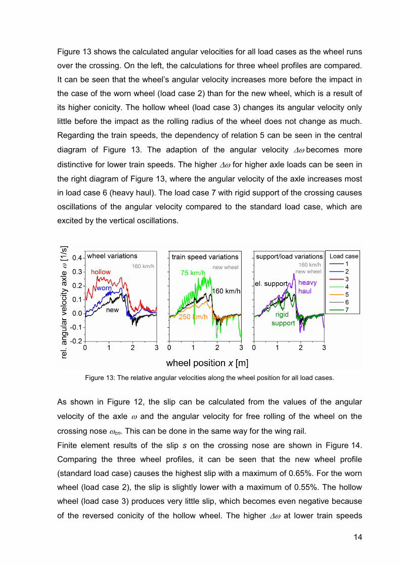
Figure 13 shows the calculated angular velocities for all load cases as the wheel runs
over the crossing. On the left, the calculations for three wheel profiles are compared.
It can be seen that the wheel’s angular velocity increases more before the impact in
the case of the worn wheel (load case 2) than for the new wheel, which is a result of
its higher conicity. The hollow wheel (load case 3) changes its angular velocity only
little before the impact as the rolling radius of the wheel does not change as much.
Regarding the train speeds, the dependency of relation 5 can be seen in the central
diagram of Figure 13. The adaption of the angular velocity becomes more
distinctive for lower train speeds. The higher for higher axle loads can be seen in
the right diagram of Figure 13, where the angular velocity of the axle increases most
in load case 6 (heavy haul). The load case 7 with rigid support of the crossing causes
oscillations of the angular velocity compared to the standard load case, which are
excited by the vertical oscillations.
Figure 13: The relative angular velocities along the wheel position for all load cases.
As shown in Figure 12, the slip can be calculated from the values of the angular
velocity of the axle and the angular velocity for free rolling of the wheel on the
crossing nose cn. This can be done in the same way for the wing rail.
Finite element results of the slip s on the crossing nose are shown in Figure 14.
Comparing the three wheel profiles, it can be seen that the new wheel profile
(standard load case) causes the highest slip with a maximum of 0.65%. For the worn
wheel (load case 2), the slip is slightly lower with a maximum of 0.55%. The hollow
wheel (load case 3) produces very little slip, which becomes even negative because
of the reversed conicity of the hollow wheel. The higher at lower train speeds

15
causes the slip to increase with decreasing train speed. In the right diagram of Figure
14, it can be seen that the slip for the rigid support (load case 7) is nearly identical to
the elastically supported standard load case. Load case 6 (heavy haul) produces also
higher slip due to the higher .
Figure 14: The slip for the seven load cases.
3.3 Contact pressure and slip of all load cases
As damage is related to the arising values of contact pressure and slip their
maximum values are shown in Figure 15 for all load cases. The position of the
plotted points indicates their type and level of loading. Towards the upper right corner
of the diagram the overall loading of the crossing increases, featuring the highest
potential for damage on the crossing nose. For the load cases of Figure 15 Table 3
gives relevant calculated load values and parameters.
Figure 15: The maximum contact pressures of the impact and the corresponding slip of all load cases
plotted in one diagram.

16
From Figures 11 and 15 it can be seen that the contact pressures in the models
reach maximum values between 3 and 6 GPa. The maximum contact pressure
clearly rises with increasing train speed. Load case 7 with rigid support produces
clearly higher contact pressures than the elastically supported standard load case.
Also, the load case 6 (heavy haul) produces higher contact pressures. The highest
maximum contact pressures of all seven load cases are produced by load case 2
with the worn wheel, where due to the worn outer wheel tread the wheel impacts
earlier on the narrow part of the crossing nose. Load case 3 with the hollow wheel,
although producing very high contact forces, shows only slightly higher contact
pressures than the standard load case.
The slip is mainly influenced by the wheel profile. For the worn wheel, the slip is
reduced compared to the standard load case. For the hollow wheel, the slip is
reduced even more because of its low wheel tread conicity. Lower train speeds
produce higher slips because of the better adaption of the angular velocity of the axle
as predicted by relation 5. Load case 6 (heavy haul) shows also higher slip than the
standard load case. This is due to the enforced adaption of the angular velocity to the
rolling radius on the wing rail by higher axle loads. It has to be remarked that not only
the slip s should be regarded but also the slip velocity, which is higher at higher train
speeds and can be calculated from the shown results.
Table 3: Results of the seven load cases. The impulse P is calculated using equation 1. The impact
force fimp, the impact position ximp, the highest contact pressure p0 and the slip s associated with the
impact are results from the finite element model.
Case Impact angle
[°]
mwheel [kg]
Impulse P [kg m/s]
Impact force
fimp [kN]
Impact position ximp [m]
p0max
[GPa] Slip s during
impact [%]
1 - standard
160 km/h 0.35 1025 278 147 1.82 3.58 0.65
2 Worn wheel 0.86 1025 684 430 1.93 5.88 0.5
3 Hollow wheel
0.66 1025 525 238 1.65 4.06 0.13 (-0.2)
4 75 km/h 0.35 1025 130 134 1.80 3.35 0.75
5 250 km/h 0.35 1025 435 321 1.82 5.02 0.55
6 Heavy haul 0.35 1500 407 260 1.82 4.67 0.8
7 Rigid support
0.35 1025 278 288 1.74 4.8 0.63
4 The role of plastic material behaviour
The crossing material plays an important role in what kind and to what extent
17
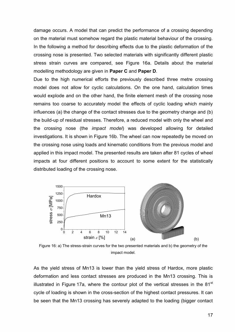
damage occurs. A model that can predict the performance of a crossing depending
on the material must somehow regard the plastic material behaviour of the crossing.
In the following a method for describing effects due to the plastic deformation of the
crossing nose is presented. Two selected materials with significantly different plastic
stress strain curves are compared, see Figure 16a. Details about the material
modelling methodology are given in Paper C and Paper D.
Due to the high numerical efforts the previously described three metre crossing
model does not allow for cyclic calculations. On the one hand, calculation times
would explode and on the other hand, the finite element mesh of the crossing nose
remains too coarse to accurately model the effects of cyclic loading which mainly
influences (a) the change of the contact stresses due to the geometry change and (b)
the build-up of residual stresses. Therefore, a reduced model with only the wheel and
the crossing nose (the impact model) was developed allowing for detailed
investigations. It is shown in Figure 16b. The wheel can now repeatedly be moved on
the crossing nose using loads and kinematic conditions from the previous model and
applied in this impact model. The presented results are taken after 81 cycles of wheel
impacts at four different positions to account to some extent for the statistically
distributed loading of the crossing nose.
0 2 4 6 8 10 12 140
250
500
750
1000
1250
1500
Mn13
Hardox
str
ess
[M
Pa
]
strain [%] (a) (b)
Figure 16: a) The stress-strain curves for the two presented materials and b) the geometry of the
impact model.
As the yield stress of Mn13 is lower than the yield stress of Hardox, more plastic
deformation and less contact stresses are produced in the Mn13 crossing. This is
illustrated in Figure 17a, where the contour plot of the vertical stresses in the 81st
cycle of loading is shown in the cross-section of the highest contact pressures. It can
be seen that the Mn13 crossing has severely adapted to the loading (bigger contact

18
patch) and thus reduced the vertical contact stresses to about 1000 MPa. For
Hardox, having plastically deformed less than Mn13, this effect is less pronounced
with vertical stresses of about 2000 MPa.
In Table 4, the results of the 81st cycle of loading are shown. Figure 17b shows a
contour plot of the residual stress component in the longitudinal direction in the
crossing nose for both materials. Under the surface, compressive stresses develop in
both materials. In the Hardox crossing nose, they are higher and closer to the surface
(-500 MPa in a depth of 3 mm) than in the Mn13 crossing nose (-200 MPa in a depth
of 6 mm). Below the area of the compressive stresses, there are some tensile
stresses which are below 150 MPa for both materials.
(a) (b)
Figure 17: a) Contour plots of the vertical stresses S22 in the cross-sections at the wheel position
producing the highest contact pressure for the two crossing materials Hardox and Mn13. It can be
seen that Hardox reaches compressive stresses of up to 2000 MPa whereas the Mn13 only reaches
stresses of about 1000 MPa. b) Contour plots of the longitudinal residual stresses in the crossing nose
after 80 cycles of loading.
Working with a hierarchical modelling system from global to a near micro description
these results can now be applied in a two-dimensional model. In addition to the
maximum contact pressure p0, the half longitudinal contact length a and the slip s are
needed as input values for a further dimensional reduction of the model.
Table 4: The loads from the 81st cycle of loading for the two crossing materials Hardox and Mn13.
Max. contact
pressure pmax [MPa]
Half contact length
a [mm]
Slip [%]
Hardox 2020 11 0.3
Mn13 1063 9.2 0.28

19
5 Studying the loading of a surface crack
Micro-models investigating crack initiation and crack growth represent one step
towards a deeper understanding of damage phenomena. The results of the contact
pressures, slips and contact patch sizes of the impact model (see Table 4) can be
transferred to a two-dimensional model that contains a surface crack (this crack
model is shown in Figure 18). With the crack model, the loading of the crack can be
calculated in terms of the crack driving forced represented by the calculation of the J-
integral (Jtip) based on the concept of configurational forces. This method also
predicts a direction of crack propagation. The modelled crack has an angle c of 30°
and a crack depth ad of 1 mm. The calculated J-integral is shown in Figure 19a for
Mn13 and 19b for Hardox as the wheel runs over it.
Figure 18: FE mesh of the crack model.
The results of the crack model are shown with and without applied residual stresses.
In Figure 19, the J- Integral Jtip is plotted over the wheel position. At a wheel position
of 0 mm, the wheel centre is directly located over the crack tip. The wheel moves
from the left to the right over the crack. For both materials, the highest Jtip values are
reached after the wheel has completely passed the crack. Regarding the results
without residual stresses, the Hardox crossing reaches with a value of 3990 J/m2 a
higher Jtip value than the Mn13 crossing with 1980 J/m2. This is caused by the lower
contact pressures of the Mn13 crossing. Applying residual stresses from the impact
model has only a small effect on the Jtip value for Mn13. For Hardox, the residual
stresses clearly reduce Jtip to a maximum value of 1560 J/m2, which is even lower
than for the Mn13 crossing. For a prediction of the crack growth rate (e.g. in nm per

20
load cycle), good measurements for crack growth are needed. As currently no
measurements under realistic mixed mode conditions exist (highly deformed surface
layers and crack propagation in the shear mode - Mode II), no final statement can be
made about the suitability of the materials for crossing noses. The model results
indicate, however, that the plastic adaption and residual stresses in the crossing can
influence the loading of cracks. It shows clearly that only a general approach and
integration of all significant parameters in the models can finally produce reliable
predictions of a crossing’s performance.
-20 -15 -10 -5 0 5 10 15 200
500
1000
1500
2000
2500
3000
3500
4000
no residual stress
with residual stress
Jtip [J/m
2]
wheel position [mm]
Hardox
(a)
-20 -15 -10 -5 0 5 10 15 200
500
1000
1500
2000
2500
3000
3500
4000
no residual stress
with residual stress
Jtip [J/m
2]
wheel position [mm]
Mn13
(b)
Figure 19: Results of the Jtip values in the crack model for c) Hardox and d) Mn13 crossing material.
6 Conclusions
Simplified models supported by results of a dynamic FE model explain how the
resulting loads on the crossing nose are caused by parameters such as the wheel
profile, trains speed etc. It is commonly assumed that damage is related to the
occurrence of contact pressure and slip. The crossing nose is the part of the crossing
where the highest amount of damage occurs. The direction in which the wheel runs
from the wing rail to the crossing nose is identified as more critical than the opposite
direction. Due to the conical wheel tread, the wheel is forced to move vertically as it
runs along the crossing. On the wing rail it moves downwards and on the crossing
nose it moves back to the initial level. There is a position in which the wheel transits
from the wing rail to the crossing nose and the change in the direction of the vertical
movement produces an impact with high contact forces. The change from the
downward movement to the upward movement during this impact (described by the
impact angle ) is an important parameter for the arising contact forces, which is
determined by the crossing and the wheel geometry. Contact forces increase with

21
increasing impact angles , axle loads, train speeds and also for stiffer vertical
supports of the crossing. Another important parameter of the impact is its longitudinal
position. Hollow wheels impact later on the crossing nose and wheels mainly worn on
the outside of the wheel tread earlier. As the crossing nose becomes narrower
towards its tip, the earlier impacts produce higher contact pressures.
The conicity of the wheel influences the described vertical movement and also
angular velocity of the wheel. The wheel always attempts to change its angular
velocity towards free rolling. The angular velocity of free rolling is determined by the
wheel radius and the train speed. A lower contact radius needs a higher angular
velocity for free rolling. The angular velocity of the wheel as it runs through a crossing
panel is thus increased on the wing rail (the contact radius of the wheel decreases)
and accelerated on the crossing nose. During the transition of the wheel from the
wing rail to the crossing nose, the wheel contacts both wing rail and the crossing
nose. From the difference in the wheel radii at these two contact points, a maximum
possible slip smax can be calculated. This difference of the radii and thus the
maximum slip is higher for higher conicities of the wheel treads- The maximum
possible slip on the crossing nose is thus higher for wheels worn on the outside of
the wheel tread and lower for hollow-worn wheels.
In reality, the wheel does not fully adapt to its angular velocity for free rolling on the
wing rail and thus less slip than smax is produced on the crossing nose. Therefore,
this adaptation is influenced by various parameters and the slip thus decreases with
higher train speed, higher rotational inertias of the axle, lower axle loads, lower wheel
radii and lower coefficients of friction between the wheel and the wing rail.
The high contact pressures calculated with the models using elastic behaviour of
wheel and rail indicate that there will be plastic deformation of the crossing nose due
to the contact loading. The amount of deformation is of course depending on the
material of the crossing. Since material selection for crossing noses is an important
issue, the effect of the plastic material behaviour is studied in a model for the
repeated loading of a crossing nose. It is shown that the plastic deformation changes
the geometry and usually lowers the contact pressures on the crossing nose (the
crossing adapts towards the wheel profile). This effect is more distinctive for
materials with lower yield stresses. Also, the plastic strains cause residual stresses in
the crossing, which are mainly compressive close to the surface. The materials with
higher yield stresses produce higher compressive residual stresses in the crossing
22
nose which are located closer to the surface than in materials with lower yield
stresses. The compressive stresses on the surface reduce crack growth rates if
cracks exist. In a model that calculates the loading of a one mm deep surface crack,
the effect of the reduced loading by the geometric adaption of the crossing and the
influence of residual stresses on the crack driving force is shown.
Acknowledgements
Financial support by the Austrian Federal Government (in particular from the
Bundesministerium für Verkehr, Innovation und Technologie and the Bundes-
ministerium für Wirtschaft und Arbeit) and the Styrian Provincial Government,
represented by Österreichische Forschungsförderungsgesellschaft mbH and by
Steirische Wirtschaftsförderungsgesellschaft mbH, within the research activities of
the K2 Competence Centre on “Integrated Research in Materials, Processing and
Product Engineering”, operated by the Materials Center Leoben Forschung GmbH in
the framework of the Austrian COMET Competence Centre Programme, is gratefully
acknowledged.
References
[1] E. Kassa, J. Nielsen, Dynamic interaction between train and railway turnout: full-
scale field test and validation of simulation models, Vehicle System Dynamics, 46
(2008) 521-534.
[2] J.F. Archard, Contact and rubbing of flat surfaces, Journal of Applied Physics, 24
(1953) 981-988.
[3] A. Ekberg, E. Kabo, Fatigue of railway wheels and rails under rolling contact and
thermal loading-an overview, Wear, 258 (2005) 1288-1300.
[4] H. Jahed, B. Farshi, M.A. Eshraghi, A. Nasr, A numerical optimization technique
for design of wheel profiles, Wear, 264 (2008) 1-10.
[5] F.D. Fischer, E.R. Oberaigner, W. Daves, M. Wiest, H. Blumauer, H. Ossberger,
The Impact of a Wheel on a Crossing, ZEVrail Glaser Annalen, 129 (2005) 336-345.
[6] H. Hertz, Über die Berührung fester elastischer Körper, Journal für die reine und
angewandte Mathematik, 92 (1881) 156-171.
[7] J. Kunz, Kontaktprobleme und ihre praktische Lösung, Konstruktion, 61 (2009)
54-58.
23
[8] F.W. Carter, On the action of a locomotive driving wheel, Proceedings of the
Royal Society of London, A 112 (1926) 151-157.
24
Paper A
A Wheel Set / Crossing Model Regarding Impact,
Sliding and Deformation- Explicit Finite Element
Approach
M. Pletz
W. Daves
H. Ossberger
Submitted to
Wear
25
A Wheel Set / Crossing Model Regarding Impact, Sliding
and Deformation- Explicit Finite Element Approach
M. Pletz1,2, W. Daves1,2, H. Ossberger3
1Materials Center Leoben Forschung GmbH, Leoben, Austria
2Institute of Mechanics, Montanuniversität Leoben, Leoben, Austria
3VAE GmbH, Zeltweg, Austria
Abstract
A dynamic finite element model for the process of a wheel passing the crossing panel
of a turnout is presented. This model accounts for the dynamic process, the elastic
deformations of the wheel and the elastic-plastic deformations of the crossing. The
axle and the second wheel are represented in terms of their influence on the angular
velocity of the wheel.
The model provides the dynamical contact forces between the wheel and the
crossing parts, the vertical wheel displacement, the development of the angular
velocity of the wheel as well as the stress fields and the plastic deformations in the
crossing. Results that indicate the loading of the surface, such as the contact
pressure and the microslip, are also provided by the model. From them, the frictional
work and the maximum of the frictional power are derived. Those values are
associated with surface damage such as wear and Rolling Contact Fatigue (RCF).
An empirical relationship between the frictional work and wear is widely used and
called Archard’s wear law. For the formation and propagation of surface cracks there
is no simple relationship.
Results for the wheel initially running on the wing rail and then impacting onto the
crossing nose (facing move) and the other direction (trailing move) are presented for
three velocities.
The presented model can help in the optimization of crossings in terms of geometry,
bedding and material, depending on the loading conditions such as train velocity,
axle load and wheel profile for both the facing and trailing move.
26
1 Introduction
Turnouts are an important part of the railway track system. They consist of a switch
and a crossing panel. In the crossing panel there is a discontinuity in the rail, which
causes a high dynamic loading. This impact loading of the crossing panel is
investigated in this work.
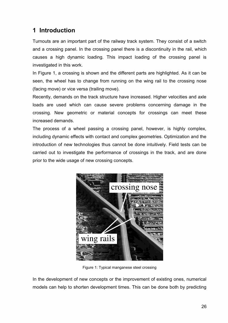
In Figure 1, a crossing is shown and the different parts are highlighted. As it can be
seen, the wheel has to change from running on the wing rail to the crossing nose
(facing move) or vice versa (trailing move).
Recently, demands on the track structure have increased. Higher velocities and axle
loads are used which can cause severe problems concerning damage in the
crossing. New geometric or material concepts for crossings can meet these
increased demands.
The process of a wheel passing a crossing panel, however, is highly complex,
including dynamic effects with contact and complex geometries. Optimization and the
introduction of new technologies thus cannot be done intuitively. Field tests can be
carried out to investigate the performance of crossings in the track, and are done
prior to the wide usage of new crossing concepts.
Figure 1: Typical manganese steel crossing
In the development of new concepts or the improvement of existing ones, numerical
models can help to shorten development times. This can be done both by predicting
27
the performance of possible design concepts and improving the understanding of the
mechanisms of loading.
According to previous finite element (FE) studies [1], the contact forces between the
wheel and the crossing nose reach values from two to four times the static wheel
load for the investigated geometrical conditions and velocities. The forces during the
impact are estimated to be more than seven times the static wheel load in analytical
calculations assuming elastic material [2].
These large contact forces between wheel and rail can cause severe damage at
crossing noses. Out of these reasons great efforts should be undertaken in
decreasing the dynamic response between wheel and track. A mass-spring model for
the analysis of an elastic-plastic beam on a foundation subjected to mass impact is
presented by Yu et al. [3]. Recent analytical investigations using mass spring models
are performed by Fischer et al. [4, 5]. Li et al. [6] developed a model in which ballast
and subgrade are modelled separately by two-dimensional finite elements to enable
the investigation of the effect of track and vehicle parameters on vertical dynamic
wheel-rail forces. Nielsen and Igeland [7] present a technique for solving problems
concerning the vertical dynamic interaction between a moving vehicle and a track
structure discretized by finite elements. With numerical calculations based on
multibody dynamics, as performed by Kassa for a train running through a complete
turnout [8], the deformability of wheel set material and rail material is usually
neglected. Following Nielsen et al. [9], multibody dynamics models fail to represent
high frequency train-track interaction. The classification of the response of the
crossing to the impact in a “high frequency contact process” and a “low frequency
bending process” is outlined in [10] and clearly shown in [11]. Andersson and
Dahlberg presented in [12] and [13] a very extensive study applying a sophisticated
system of finite elements for the turnout.
Stress and strain analyses are the key to understand and predict the wear and
fatigue behaviour of contacting and impacting bodies. Johansson [14] performed a
calculation on a section of a crossing nose loaded by a Hertzian contact pressure
distribution. There exists a lot of work in the literature on the topic of wheel-rail
contact calculations. The majority of them use simplifications. Saulot and Baillet [15]
use a two-dimensional FE model to investigate contact dynamic instabilities. A three-
dimensional FE model of a rail, on which they applied moving contact pressure
distributions according to Hertz [16] and the analysis tool CONTACT [17], is

28
presented by Ringsberg and Josefson [18]. Sladkowski and Sitarz [19] as well as
Telliskivi and Olofsson [20] applied global forces calculated by multibody dynamics
programs to the wheel centre of their three-dimensional FE models of wheel and rail.
The cyclic response of a crossing is analysed by Yan et al. [21]. A very sophisticated
three-dimensional dynamic simulation of a wheel impacting on the rail joint region is
performed by Wen et al. [22]. The common criticism on the FE studies of Yan et al.
as well as of Wen et al. might be that the rolling of the wheel is neglected. Finite
element simulations, reflecting the three-dimensional contact combined with
dynamical rolling of the three-dimensionally modelled wheel and rail including elastic-
plastic material properties are done by Wiest et al. in [1, 23, 24, 25].
A representation of the realistic geometry of wing rail and crossing nose was
archived by the authors due to increased computing power in combination with the
established knowledge about modelling the complicated and highly dynamic
transition process.
In [26, 27], a model containing the realistic geometry of the crossing parts and a
representation of the whole wheel set is presented. The results of the facing move
are presented there.
The presented model, being based on an explicit finite element formulation, has
certain limitations:
high calculation times (5-48 h/cycle) compared to multibody system methods,
only a length of 3 metres of the crossing is modelled,
assumptions about the wheel position (fixed lateral position, no steering of the
bogie).
Using the present model allows for calculating the realistic slipping between the
wheel and the wing rail and the crossing nose depending on
the angular velocity of the wheel,
the contact positions of the wheel on the crossing parts (wing rail and/or
crossing nose),
the geometry of the involved parts,
the plastic material behaviour of the crossing parts,
the inertia of the bodies.
The dynamical loading of the crossing in combination with the slip between the wheel
and the crossing parts can lead to wear, rolling contact fatigue and severe plastic
deformation of the crossing. The dynamic situation can be illustrated by the

29
developments of the contact forces and the angular wheel velocity. Damage,
however, is related to the local contact situation with the pressure and microslip (local
tangential velocity difference of contacting surfaces) that cause stresses and plastic
strains in the crossing parts.
In this work, the accumulated equivalent plastic strain after one crossover is
calculated to indicate the loading of the material in terms of plastic deformation, e.g.
ratchetting.
The frictional work is widely used to calculate wear, e.g. based on Archard’s wear law
[28]. It is thus evaluated in the presented model.
Archard’s law, however, is based on experimental data and a wear coefficient is only
valid for one microslip/pressure combination. Krause and Poll [29] state that the
frictional power per surface area indicates the shift between different wear
mechanisms with different wear coefficients. The maximum occurring frictional power
per surface area is thus also evaluated in this work.
2 Finite Element Model
2.1 Setup of the model
The finite element model represents the full three-dimensional geometry of one
wheel, the crossing nose and the wing rails (see Figure 2a-d). The crossing model
represents a manganese cast crossing of the standard design 760-1:15 for a UIC60
rail. The wheel (UIC-ORE 1002 Profile) is modelled using elastic material properties
save for the hub with a radius of 116.5 mm which is considered rigid (see Figure 2d).
To ensure a proper description of the dynamic process, the rigid plate is used for
representing the mass of the remaining part of the first wheel and the moment of
inertia of the remaining part of the first wheel, the axle and the second wheel.
In Figure 3, the mechanical model illustrating the assumptions of the presented
crossover calculation is shown. The parts of the model which are represented by
explicit finite elements are dark grey and denoted by (Ia) and (Ib). The bottom of the
crossing is rigidly connected to a parallel spring/damper combination, giving a rough
representation of the crossings bedding (II). For the initial positioning of the wheel on
the rail, the wheel centre is connected to a vertical damping element that removes
initial oscillations of the contact force (III), as described in [23]. An initial damping
coefficient kp of 4x10⁶ Ns/m is used and then reduced to a value of 53 000 Ns/m,

30
which is a realistic value for the primary suspension of the bogie. The wheel centre is
connected to a frictional element (rotation around the x- axis) that represents the
second wheel and is described in section 2.2.
(a) (b)
(c) (d)
Figure 2: Finite element model: (a) Wheel and crossing, (b) cross section, (c) crossing parts and
(d) wheel mesh.
In the centre of the wheel, the used coordinate system is shown. The x-axis denotes
the lateral direction, y the vertical direction and z the longitudinal. The reference point
of the rigid axle of the wheel is positioned in the origin of the coordinate system. In
this point, loads are applied on the wheel. The wheel’s rotation in the z and y
direction is disabled. Also, the wheel is held in the x (lateral) direction on a position
that corresponds to the second wheel running along the check rail. In the z
(longitudinal) direction, the wheel centre, the vertical dashpot and the rotational
frictional element are moved with a constant velocity. A point mass is attached to the
centre of the wheel so that the wheel has a total mass of 1025 kg. The moment of
inertia of the two wheels and the axle about the x-axis of 135.5 kgm2 is provided at
the reference point.
In the x- direction, an initial angular velocity is applied in the wheel around its centre.
31
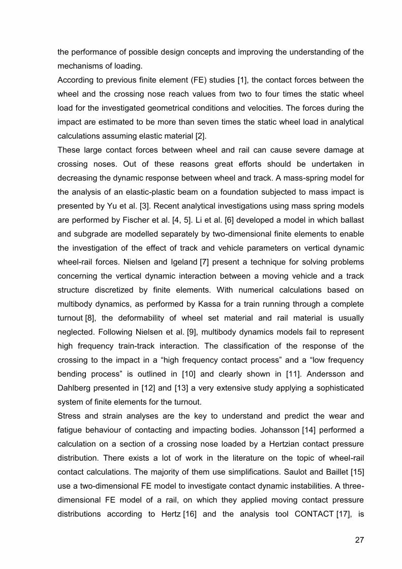
The angular velocity during the transition process is not constrained, thus
representing a free rolling wheel.
Figure 3: The mechanical model for the wheel and the crossing. (I) The parts of the wheel and the
crossing that are calculated using finite elements (dark grey), (II) the representation of the crossing’s
bedding, (III) the vertical damping element attached to the wheel, (IV) the rotational frictional element
with a schematic moment- angular velocity curve and (V) the coordinate system used in the model.
The manganese steel crossing is modelled with a length of 3 metres using about
100 000 elements. The total number of elements in the model amounts to 250 000.
The calculations are performed using the finite element code ABAQUS/Explicit [30].
The mesh-size of the hexahedral elements in contact is not larger than 3 mm. This
mesh size ensures a correct description of the contact forces and slipping behaviour.
However, it will still create some quantitative errors in the results of stresses and
strains. The used material data for the wheel (elastic) and crossing parts (Mn13) are
printed in Table 1. A friction coefficient of 0.3 is assumed between wheel and
crossing parts.
The used static wheel load is 79 700 N, corresponding to an axle load of 14.2 tons.
The mass of the wheel including half of the axle is set to 1025 kg. The whole mass of
the crossing parts, denoted in Figure 3 as (Ib), adds up to 680 kg.

32
Property Manganese
steel (Mn13)
Wheel
(elastic)
Young’s modulus [GPa] 190 210
Poisson’s ratio [1] 0.3 0.3
Density [kg/m³] 7800 7800
Yield stress [MPa] 360 -
Table 1: Material properties from the tension test.
2.2 Simplified model of the second wheel on the regular rail
A full finite element model of the whole axle with both wheels would lead to
unacceptable computation times. From the second wheel, only the effect on the
angular velocity of the axle is relevant. Therefore, the second wheel is represented
using one single element. This element possesses an angular frictional behaviour,
which is described in the following paragraphs.
It is assumed that the second wheel is running along the check rail, which defines the
lateral position of the wheel set. Since the regular cross-section of the rail does not
change in the longitudinal direction, the second wheel runs with a constant contact
radius R2 throughout the process. With v0 being the translational velocity of the
wheel, a rotational velocity of 2,0 = v0/R2 corresponds to the free rolling of the
second wheel. Any other rotational velocity produces frictional forces, which tend to
change the rolling velocity of the wheel set.
When the whole contact patch between the second wheel and the rail is in full slip,
the second wheel produces a torsional moment M on the axle that is given by
M = μ F0 R2 with μ being the coefficient of friction and F0 the static vertical load on the
second wheel. With small deviations of the rotational velocity of the axle from 2,0,
stick and slip regions within the contact patch develop. A traction–slip relationship
has thus to be used for the calculation of the torsional moment M.
To obtain a satisfactory estimate of M on the axle, the second wheel and the rail
have been modelled in a separate but similar finite element investigation. Using this
model, a fixed rotational velocity of the wheel leads to a corresponding moment on
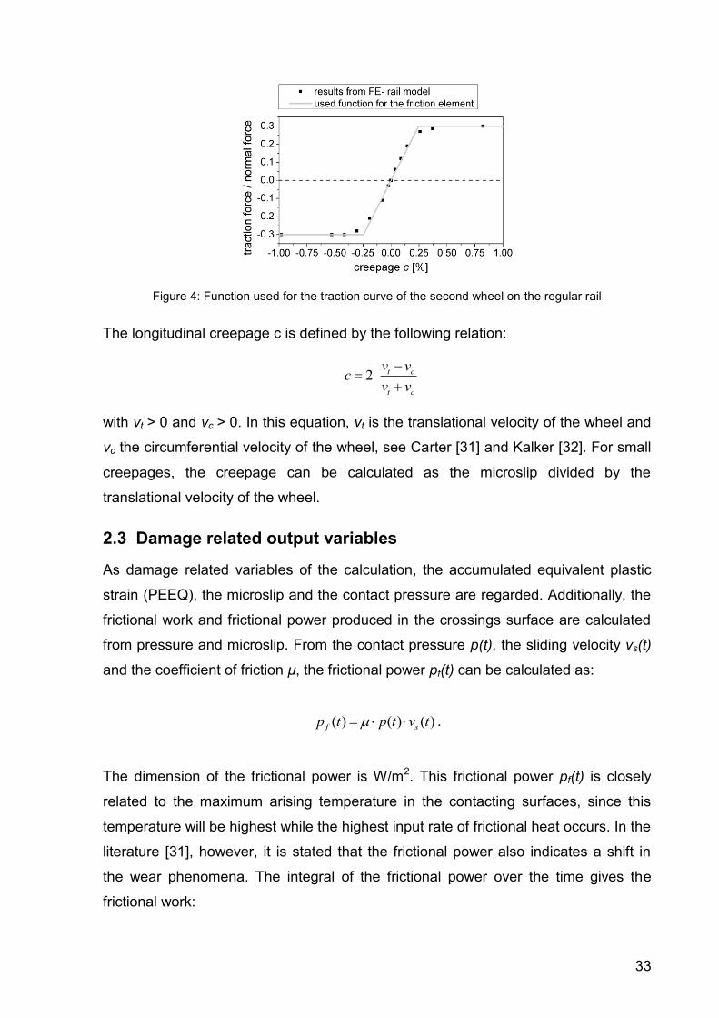
the axle. In Figure 4, the results for this model and the linearised function used for
the described frictional element are plotted.
33
Figure 4: Function used for the traction curve of the second wheel on the regular rail
The longitudinal creepage c is defined by the following relation:
2 t c
t c
v vc
v v
with vt > 0 and vc > 0. In this equation, vt is the translational velocity of the wheel and
vc the circumferential velocity of the wheel, see Carter [31] and Kalker [32]. For small
creepages, the creepage can be calculated as the microslip divided by the
translational velocity of the wheel.
2.3 Damage related output variables
As damage related variables of the calculation, the accumulated equivalent plastic
strain (PEEQ), the microslip and the contact pressure are regarded. Additionally, the
frictional work and frictional power produced in the crossings surface are calculated
from pressure and microslip. From the contact pressure p(t), the sliding velocity vs(t)
and the coefficient of friction μ, the frictional power pf(t) can be calculated as:
( ) ( ) ( )f sp t p t v t .
The dimension of the frictional power is W/m2. This frictional power pf(t) is closely
related to the maximum arising temperature in the contacting surfaces, since this
temperature will be highest while the highest input rate of frictional heat occurs. In the
literature [31], however, it is stated that the frictional power also indicates a shift in
the wear phenomena. The integral of the frictional power over the time gives the
frictional work:
34
( )f f
t
w p t dt .
The frictional work is widely associated with wear. Its dimension is J/m2. In Archard’s
wear law [28], for example, the wear depth equals the frictional work times an
empirical wear constant divided by the hardness of the material.
3 Results and Discussion
3.2 Dynamic results of the model
In Fig 5, contact forces for the three trains speeds of 75 km/h, 160 km/h and
250 km/h and both facing and trailing move are shown. For the velocity of 160 km/h,
the vertical displacements of the wheel centre and the crossing is shown in Figure 6.
The results are plotted over the position of the wheel, which ranges from 0 m (wheel
on the straight part of the wing rail) to 3 m (wheel on the crossing nose). For all
cases, the initial placing of the wheel on the wing rail causes oscillations in the
contact force. Vertical displacements of the wheel, however, are only small in this
area.
In Figure 5 (a), (c) and (e), the results for the contact force in the facing move are
shown. In this direction of passing, first oscillations are excited at a wheel position of
0 m, which depend on the train speed. At a wheel position of 0.2 m, the wing rail
starts to deviate. For the wheel, featuring a conical wheel tread, this causes a
vertical, downward movement that produces some oscillations in the contact force,
depending on the train speed. The amplitudes of these oscillations are reduced along
the next metre, caused by dissipation in the vertical damping element of the wheel
and the crossings bedding. Plastic deformation plays only a small role in this
dissipation. As the wheel approaches the crossing nose (1 m – 1.75 m), some more
oscillations occur. They are caused by another change in the vertical movement of
the wheel, as it can be seen in Figure 6(a). At a velocity of 250 km/h, the wheel in
this area even loses contact with the wing rail - it bounces.
At a wheel position of about 1.75 m, the wheel impacts onto the crossing nose. As
the wheels vertical velocity has to change abruptly, oscillations of the contact force
arise. Those oscillations, however, are reduced because the wheel is still contacting
the wing rail as it impacts onto the crossing nose. In the model with 250 km/h, this
effect is only small, and very high contact forces arise. Dissipation in the vertical
35
damper and the contact patch again reduces these oscillations in the following 0.5 m.
At a wheel position of 2.7 m, again some oscillations are excited due to the ending
ramp of the crossing in the model.
In Figure 5 (b), (d) and (f), results for the contact forces in the trailing move are
presented. The train moves in the opposite direction in this case (from right to left in
the diagram) and the initial placing of the wheel is on the crossing nose with a wheel
position of 2.9 m. At a wheel position of 2.7 m, there is a kink in the crossing nose,
causing a downward movement of the wheel and an excitation of oscillations. As the
wheel approaches the wing rail, these oscillations become smaller. The wheel
changes from the crossing nose to the wing rail at a wheel position of about 1.75 m,
producing an impact. At a wheel position of 0.2 m, some oscillations occur due to a
change in the rolling plane of the wing rail, which have no significance for the loading
of the crossing nose.
As an elastic bedding of the crossing is used in the model, both the vertical
displacement of the wheel centre and of the whole crossing can be evaluated. The
vertical movement of the crossing is determined by the contact force between the
wheel and the crossing, the crossing mass and its bedding. In Figure 6, results of
these vertical movements are shown for a train speed of 160 km/h. As the wing rail
starts to deviate at a wheel position of 0.2 metres, the wheel starts to lower its vertical
position in the facing move (Figure 6a). Up to this position, the spring in the bedding
is compressed due to the vertical contact force. As the contact force drops at
0.2 metres, the spring can uncompress and the crossing’s vertical position rises by
about 0.2 mm. As the wheel impacts on the crossing nose (at a wheel position of 1.8
metres), the wheel centre moves upward again. As this impact produces increased
vertical contact forces, the crossing is pressed down by about 0.8 mm, compressing
the spring of the bedding. Towards the end of the model (x = 3 m), the crossing’s and
the wheel’s vertical positions approach a similar level as at the start of the simulation.
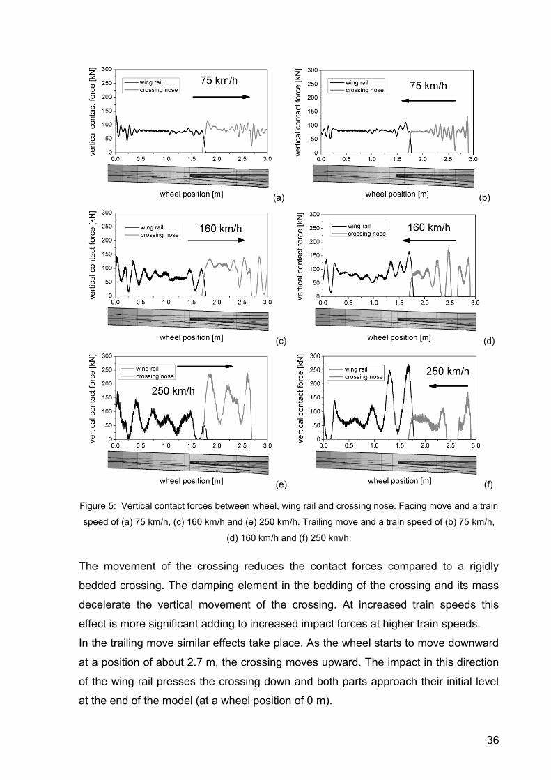
36
(a) (b)
(c) (d)
(e) (f)
Figure 5: Vertical contact forces between wheel, wing rail and crossing nose. Facing move and a train
speed of (a) 75 km/h, (c) 160 km/h and (e) 250 km/h. Trailing move and a train speed of (b) 75 km/h,
(d) 160 km/h and (f) 250 km/h.
The movement of the crossing reduces the contact forces compared to a rigidly
bedded crossing. The damping element in the bedding of the crossing and its mass
decelerate the vertical movement of the crossing. At increased train speeds this
effect is more significant adding to increased impact forces at higher train speeds.
In the trailing move similar effects take place. As the wheel starts to move downward
at a position of about 2.7 m, the crossing moves upward. The impact in this direction
of the wing rail presses the crossing down and both parts approach their initial level
at the end of the model (at a wheel position of 0 m).
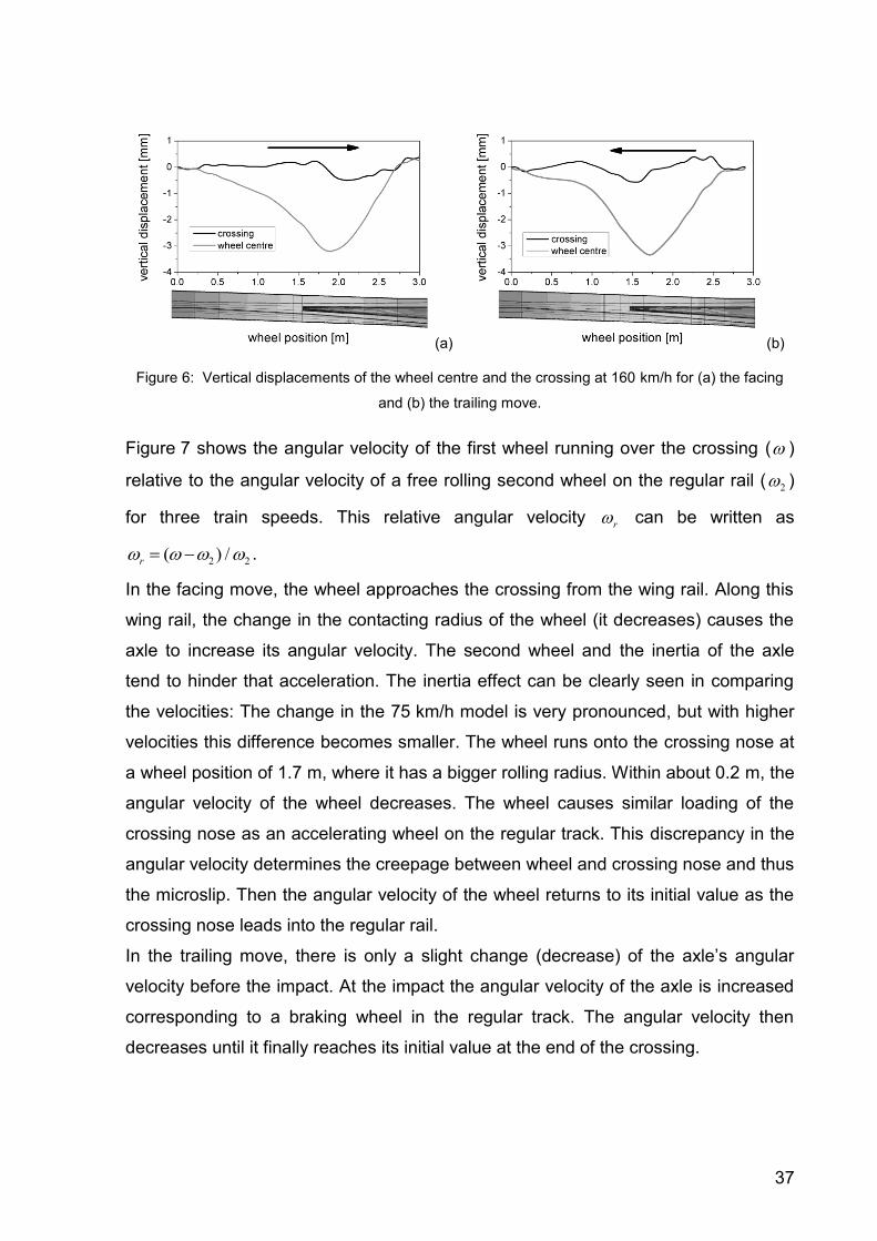
37
(a) (b)
Figure 6: Vertical displacements of the wheel centre and the crossing at 160 km/h for (a) the facing
and (b) the trailing move.
Figure 7 shows the angular velocity of the first wheel running over the crossing ( )
relative to the angular velocity of a free rolling second wheel on the regular rail ( 2 )
for three train speeds. This relative angular velocity r can be written as
2 2( ) /r .
In the facing move, the wheel approaches the crossing from the wing rail. Along this
wing rail, the change in the contacting radius of the wheel (it decreases) causes the
axle to increase its angular velocity. The second wheel and the inertia of the axle
tend to hinder that acceleration. The inertia effect can be clearly seen in comparing
the velocities: The change in the 75 km/h model is very pronounced, but with higher
velocities this difference becomes smaller. The wheel runs onto the crossing nose at
a wheel position of 1.7 m, where it has a bigger rolling radius. Within about 0.2 m, the
angular velocity of the wheel decreases. The wheel causes similar loading of the
crossing nose as an accelerating wheel on the regular track. This discrepancy in the
angular velocity determines the creepage between wheel and crossing nose and thus
the microslip. Then the angular velocity of the wheel returns to its initial value as the
crossing nose leads into the regular rail.
In the trailing move, there is only a slight change (decrease) of the axle’s angular
velocity before the impact. At the impact the angular velocity of the axle is increased
corresponding to a braking wheel in the regular track. The angular velocity then
decreases until it finally reaches its initial value at the end of the crossing.
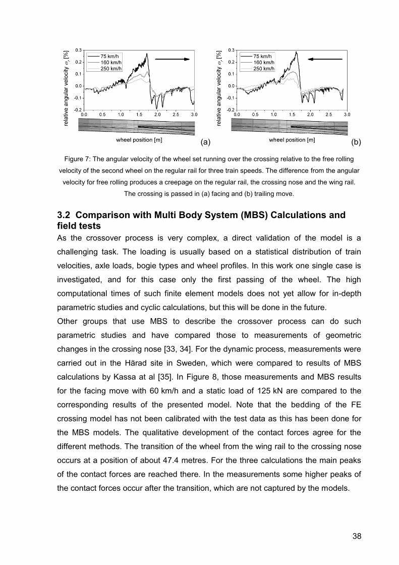
38
(a) (b)
Figure 7: The angular velocity of the wheel set running over the crossing relative to the free rolling
velocity of the second wheel on the regular rail for three train speeds. The difference from the angular
velocity for free rolling produces a creepage on the regular rail, the crossing nose and the wing rail.
The crossing is passed in (a) facing and (b) trailing move.
3.2 Comparison with Multi Body System (MBS) Calculations and field tests
As the crossover process is very complex, a direct validation of the model is a
challenging task. The loading is usually based on a statistical distribution of train
velocities, axle loads, bogie types and wheel profiles. In this work one single case is
investigated, and for this case only the first passing of the wheel. The high
computational times of such finite element models does not yet allow for in-depth
parametric studies and cyclic calculations, but this will be done in the future.
Other groups that use MBS to describe the crossover process can do such
parametric studies and have compared those to measurements of geometric
changes in the crossing nose [33, 34]. For the dynamic process, measurements were
carried out in the Härad site in Sweden, which were compared to results of MBS
calculations by Kassa at al [35]. In Figure 8, those measurements and MBS results
for the facing move with 60 km/h and a static load of 125 kN are compared to the
corresponding results of the presented model. Note that the bedding of the FE
crossing model has not been calibrated with the test data as this has been done for
the MBS models. The qualitative development of the contact forces agree for the
different methods. The transition of the wheel from the wing rail to the crossing nose
occurs at a position of about 47.4 metres. For the three calculations the main peaks
of the contact forces are reached there. In the measurements some higher peaks of
the contact forces occur after the transition, which are not captured by the models.
39
(a) (b)
(c) (d)
Figure 8: Comparison of the vertical contact forces of (a) the presented model with (b) measurements
in the track and results of multi-body calculations with the commercial code (c) GENSYS and (d)
DIFF3D. Static load of 125 kN and train velocity of 60 km/h in the facing move, see also [35]
3.3 Results for the damage related output variables
In Figure 9, variables that indicate the loading of the crossing nose and the wing rail
are shown for the 160 km/h model and the facing move. A close-up of the area where
the transition of the wheel takes place is displayed. In Figure 9(a) and 9(b), the
frictional work and the maximum frictional power are plotted. These output variables
are associated with wear and surface damage, and reach their maximum at the
crossing nose. The frictional work has a maximum of 0.019 J/mm2 and the frictional
power is 156 W/mm2.
Figure 9(c) shows the maximum of the arising microslip. It can be seen that the
values are highest at a position on the crossing nose (0.7 m/s) where the wheel
impacts on it, but not so pronounced as the frictional work and power, which also
accounts for the high contact pressures in that region.
In Figure 9(d), the accumulated equivalent plastic strain (PEEQ) is shown as a
contour plot on the crossing parts, values of which are clearly higher on the crossing
nose with a maximum of 3.5 %. Comparing the vertical contact forces with this PEEQ
it can be seen that not only the value of the vertical contact force but also the contact
geometry determines the plastic strains. On the tip of the crossing nose, for example,
40
the same vertical load causes much higher plastic deformations than on the broader
part of the nose or the wing rail.
(a) (b)
(c) (d)
Figure 9: Results for the 160 km/h model and facing move of the wheel: Contour plots at the surface of
the crossing nose of (a) frictional work, (b) max. frictional power, (c) max. microslip and
(d) accumulated equivalent plastic strain (PEEQ).
The same output can be shown in diagrams containing the maximum of the output
variables in the cross-sections of the crossing, which is done in Figure 10. For the
frictional power and the frictional work, this would be a certain position on the surface
of the crossing parts. For the PEEQ, the maximum is usually beneath the surface.
It can be seen that the maximum of the output variables is situated in the area where
the wheel changes from the wing rail to the crossing nose or vice versa. The
geometric situation at the tiny tip of the crossing nose and the fact that the wheel
contacts the wing rail with its outer edge of the tread causes increased loading that is
not indicated by the contact forces alone.
The frictional work and the frictional power show a similar behaviour for both
directions. Only a slight increase at the position where the impact occurs can be
determined.
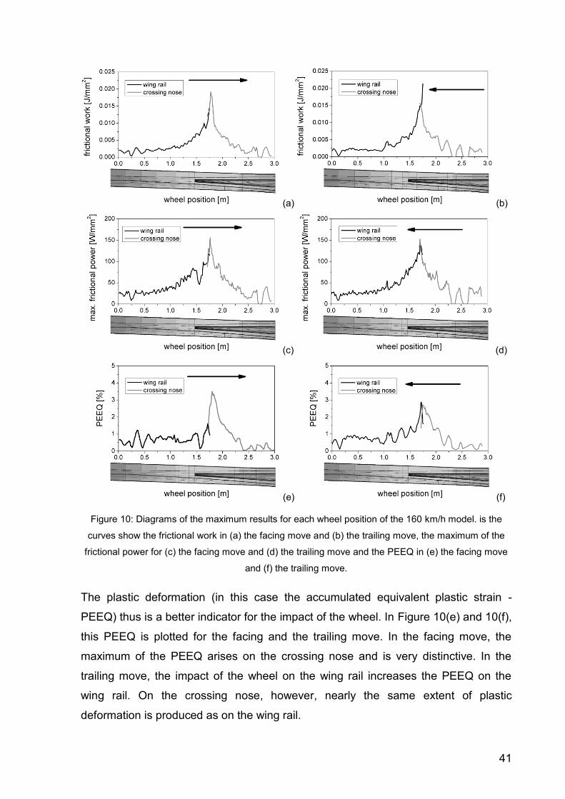
41
(a) (b)
(c) (d)
(e) (f)
Figure 10: Diagrams of the maximum results for each wheel position of the 160 km/h model. is the
curves show the frictional work in (a) the facing move and (b) the trailing move, the maximum of the
frictional power for (c) the facing move and (d) the trailing move and the PEEQ in (e) the facing move
and (f) the trailing move.
The plastic deformation (in this case the accumulated equivalent plastic strain -
PEEQ) thus is a better indicator for the impact of the wheel. In Figure 10(e) and 10(f),
this PEEQ is plotted for the facing and the trailing move. In the facing move, the
maximum of the PEEQ arises on the crossing nose and is very distinctive. In the
trailing move, the impact of the wheel on the wing rail increases the PEEQ on the
wing rail. On the crossing nose, however, nearly the same extent of plastic
deformation is produced as on the wing rail.

42
3.4 Comparison of the results for both directions and three
velocities
In Table 2, the maxima of the different results for the three train velocities and both
directions of passing are compared. The maximum of the vertical contact force due to
the impact of the wheel on the crossing nose considerably increases with increasing
velocity, reaching a value of 242 kN (facing move) and 271 kN (trailing move) at
250 km/h. The dynamic factor d representing the ratio of the impact force to the static
load (79.7 kN) reaches values of 1.41 up to 3.4. The maximum of the accumulated
equivalent plastic strain (PEEQ) amounts to 2.96 % (facing move) and 2.42 %
(trailing move) for the model with 75 km/h. For the facing move, it increases with
increasing velocity to 3.5 % (160 km/h) and 5.77 % (250 km/h). Regarding the trailing
move it shows only a small increase of the maximum of the PEEQ to 2.7 % (160
km/h) and 2.95 % (250 km/h). The facing move causes the highest values of the
PEEQ always in the crossing nose. For the trailing move the PEEQ at 75 km/h also
leads to high values in the crossing nose. Due to the increased impact forces at the
wing rail at higher velocities (160 km/h and 250 km/h) the PEEQ becomes higher in
the wing rail than in the crossing nose.
Note that these plastic strains are calculated for the first passing of a wheel, when
neither the material has previously hardened or softened nor the crossing nose has
adapted its geometry to the loading. Therefore, the first plastic strain increment is
very high compared to later progressive plastic deformation after several thousands
of wheels have passed the crossing.
The microslip vs, defined as the relative velocity between two contacting points, also
increases with the train velocity. On the wing rail and the crossing nose about the
same maxima of microslips arise. The creepage is higher in the 75 km/h model than
for the other two train speeds, where nearly the same creepages arise. This is
caused by the velocity- dependent adaption of the wheel’s angular velocity to the
rolling situation on the wing rail before running onto the crossing nose. At lower
speeds the angular inertia of the axle has the smallest effect and thus the adaption
occurs fast causing a bigger misfit in the rotational velocity of the wheel at the
change to the crossing nose. This effect can be seen in Figure 7.

43
Train speed 75 km/h 160 km/h 250 km/h
Move facing trailing facing trailing facing trailing
Max. vertical contact force at impact [kN] 116 112 136 166 242 271
Dynamic factor 1.45 1.41 1.55 2.08 3.04 3.4
Max. acc. equiv. plastic strain- crossing nose
[%] 2.96 2.42 3.5 2.7 5.77 2.95
Max. acc. equiv. plastic strain- wing rail [%] 1.23 1.53 1.6 2.88 1.23 3.62
Highest microslip vs [m/s] 0.54 0.59 0.69 0.55 1.11 0.91
Highest creepage c vs/vt [%] 2.59 2.82 1.55 1.24 1.59 1.31
Maximum frictional work wf [J/mm2] 0.0215 0.0185 0.0192 0.0158 0.0141 0.0153
Maximum frictional power pf [W/mm2] 111 139 156 181 194 220
Table 2: The maxima of the relevant output variables for three train speeds and two directions of
passing.
Due to this inertia effect that causes a decrease in the creepage with increasing
velocity the calculated maximum frictional work for the facing and the trailing move
decreases. The highest values of the frictional work are calculated in the crossing
nose for the facing move with 75 km/h as 0.0215 J/mm2. Since the maximum of the
frictional power depends on the highest amount of microslip, the frictional power
increases with increasing train velocity. The frictional power reaches values of up to
220 W/mm2 on the wing rail for the trailing move with 250 km/h.
4 Conclusions
A dynamic finite element model for a wheel set passing a crossing is developed. The
parameters of this model are the axle load, the passing velocity, the passing
direction, the geometry and the material behaviour of wheel and crossing. There are
two aspects of the process, which are of special interest: The vertical impact of the
wheel and the change in the angular velocity of the wheel.
The model provides results for the contact forces between the wheel and the
crossing parts. The impact of the wheel on the crossing nose can thus be studied.
The crucial parameter for that impact is the angle between the velocity vectors when
the wheel changes from the wing rail to the crossing nose. This is illustrated by the
results for the vertical displacement of the wheel centre. Additionally, the model
calculates the angular velocity of the wheel, which increases in the area of the wing
rail and decreases as the wheel runs onto the crossing nose.

44
The impact of the wheel on the crossing nose is associated with high contact
stresses and high plastic deformations. The change in the angular velocity of the
wheel, on the other side, is associated with slip between the wheel and the crossing
parts.
The contact pressure and the microslip are important variables for the surface
damage of the crossing. High microslips in combination with high contact pressures
can lead to wear and rolling contact fatigue. The frictional work and the maximum of
the frictional power are measures for this damage and are thus evaluated in the
presented model.
In crossings damage is observed in areas where the presented model calculates the
highest frictional powers and frictional works. Empirical laws state that the frictional
work is proportional to the wear depth. A detailed explanation of the interrelation
between frictional work, frictional power and damage still has to be established using
micro-models and experiments.
The presented model provides a practical tool for the optimization of crossings in
terms of geometry, bedding and material. The mechanisms that cause the loading of
the critical parts can be described, providing a better understanding of the process.
New crossing concepts can be investigated before manufacturing prototypes and
conducting field tests, thus reducing the development time. Serving as a tool for track
engineers, the model will be able to explain the influence of velocity, bedding, axle
load and wheel profiles on the crossings lifetime.
Acknowledgements
Financial support by the Austrian Federal Government (in particular from the
Bundesministerium für Verkehr, Innovation und Technologie and the
Bundesministerium für Wirtschaft und Arbeit) and the Styrian Provincial Government,
represented by Österreichische Forschungsförderungsgesellschaft mbH and by
Steirische Wirtschaftsförderungsgesellschaft mbH, within the research activities of
the K2 Competence Centre on “Integrated Research in Materials, Processing and
Product Engineering”, operated by the Materials Center Leoben Forschung GmbH in
the framework of the Austrian COMET Competence Centre Programme, is gratefully
acknowledged.
The authors specially thank Elias Kassa for providing the data for the MBS and field
measurement comparison, shown in section 3.2.
45
References
[1] M. Wiest, W. Daves, F.D. Fischer and H. Ossberger: ZEVrail Glas. Ann., 2005,
vol. 129 (11-12), pp 461-467 (in German).
[2] F.D. Fischer, H. Steiner and R. Schossmann: ETR (Eisenbahntechnische
Rundschau), 1979, vol. 28 (7/8), pp 597-602 (in German).
[3] T.X. Yu, X.W. Chen and Y.Z. Chen: Computers and Structures, 2002, vol. 80,
pp 1965-1973.
[4] F.D. Fischer, E.R. Oberaigner, W. Daves, M. Wiest, H. Blumauer and H.
Ossberger: ZEVrail Glas. Ann., 2005, vol. 129 (8), pp 336-345.
[5] F.D. Fischer, W. Daves and H. Dirschmid: ZEVrail Glas. Ann., 2005, vol. 132,
pp 187-190.
[6] M.X.D. Li, T. Ekevid and N.-E. Wiberg: An Integrated Vehicle-Track-Ground
Model for Investigating the Wheel/Rail Dynamic Forces due to High Axle
Loads, Proceedings of the 6th International Conference on Contact Mechanics
and Wear of Rail/Wheel Systems, Gothenburg, Sweden, 2003, pp 295-300.
[7] J.C.O. Nielsen and A. Igeland: J. Sound Vibr., 1995, vol. 187 (5), pp 825-839.
[8] E. Kassa: Simulation of Dynamic Interaction between Train and Turnout,
Licentiate Thesis, Chalmers University of Technology, Department of Applied
Mechanics, Gothenburg, Sweden, 2004.
[9] J.C.O. Nielsen, R. Lundén, A. Johansson and T. Vernersson: Vehicle Syst.
Dyn., 2003, vol. 40 (1-3), pp 3-54.
[10] H.H. Jenkins, J.E. Stephenson, G.A. Clayton, G.W. Morland and D. Lyon:
Railway Eng. J., 1974, vol. 3, pp 2-16.
[11] S. Iwnicki: Fatigue Fract. Engng. Mater. Struct., 2003, vol. 26 (10), pp 887-
900.
[12] C. Andersson and T. Dahlberg: Proc. Instn. Mech. Engrs., Part F. J. Rail Rapid
Transit, 1998, vol. 212, pp 123-134.
[13] C. Andersson and T. Dahlberg: Vehicle Syst. Dyn. Suppl., 1999, vol. 33, pp
131-142.
[14] G. Johansson, M. Ekh and K. Runesson: Int. J. Plasticity, 2005, vol. 21, pp
955-980.
[15] Saulot and L. Baillet, Finite Element Simulation of Wheel-Rail Contact
Dynamic Instabilities Under Sliding Conditions, Proceedings of World
Tribology Congress III, Washington, D.C., USA, 2005, pp 249-250.

46
[16] K.L. Johnson: Contact Mechanics, Cambridge University Press, Cambridge,
UK, 1985.
[17] J.J. Kalker: Three-dimensional Elastic Bodies in Rolling Contact, Kluwer,
Dordrecht, the Netherlands, 1990.
[18] J. Ringsberg and B.L. Josefson: Proc. Instn. Mech. Engrs., Part F. J. Rail
Rapid Transit, 2001, vol. 215, pp 243-159.
[19] Sladkowski and M. Sitarz: Wear, 2005, vol. 258, pp 1217-1223.
[20] T. Telliskivi and U. Olofsson: Proc. Instn. Mech. Engrs., Part F. J. Rail Rapid
Transit, 2001, vol. 215, pp 65-72.
[21] W.Y. Yan, T. Antretter, F.D. Fischer and H. Blumauer: “Numerical Analysis of
the Cyclic Response of a Crossing Component in a Switch”, in “Proceedings of
the XIX. Verformungskundliches Kolloquium”, Montanuniversität Leoben,
Austria, 2000, pp 78-83.
[22] Z. Wen, X. Jin and W. Zhang: Wear, 2005, vol. 258, pp 1301-1309.
[23] M. Wiest: Modelling of Wheel-Rail/Crossing Interactions, 12, Nr. 642, VDI-
Verlag, Düsseldorf, 2007.
[24] M. Wiest, Kassa, E., Daves, W., Nielsen, J.C.O. and H. Ossberger: Wear,
2008, vol. 265, pp 1439-1445.
[25] M. Wiest, Daves, W., Fischer, F.D. and Ossberger, H.: Wear, 2008, vol. 256,
pp 1431-1438.
[26] M. Pletz, W. Daves, F.D. Fischer and H. Ossberger, “A Dynamical Wheel Set:
Crossing Model Regarding Impact, Sliding and Deformation”, in “Proceeding at
the 8th International Conference on Contact Mechanics and Wear of
Rail/Wheel Systems”, Florence, Italy, pp 801-809, 2009.
[27] M. Pletz, W. Daves and H. Ossberger, “Dynamic Finite Element Model of a
Wheel Passing a Crossing Nose”, in “Proceeding at the The Tenth
International Conference on Computational Structures Technology”, Valencia,
Spain, 2010.
[28] J.F. Archard: J. of Appl. Phys., 1953, vol. 24, pp 981-988.
[29] H. Krause and G. Poll: Wear, 1986, vol. 113, pp 103-122.
[30] Abaqus, ABAQUS User’s Manual, version 6.7, 2009, www.abaqus.com.
[31] F.W. Carter: Proc. R. Soc., 1926, vol. A112, pp. 151-157.
[32] J.J. Kalker: Wear, 1991, vol. 144, pp 243-261.
[33] A. Johansson, B. Palsson, M. Ekh, J.C.O. Nielsen, M.K.A. Ander, J.
47
Brouzoulis and E. Kassa: Wear, vol. 271, 2011, pp 472-481.
[34] D. Nicklisch, J. C. O. Nielsen, M. Ekh, A. Johansson, B. Pålsson, J. M.
Reinecke and A. Zoll, “Simulation of wheel–rail contact and subsequent
material degradation in switches & crossings”, in “Proceedings of the 21st
International Symposium on Dynamics of Vehicles on Roads and Tracks”,
Stockholm, Sweden, 2009.
[35] E Kassa and J C O Nielsen: Vehicle Syst. Dyn. Suppl., 2008, vol. 46, pp 521-
534.

48
Paper B
A Wheel Passing a Crossing Nose- Dynamic
Analysis under High Axle Loads using Finite
Element Modelling
M. Pletz
W. Daves
H. Ossberger
in
Proceedings of the Institution of Mechanical Engineers, Part F: Journal of Rail and
Rapid Transit, (2012)
49
A Wheel Passing a Crossing Nose- Dynamic
Analysis under High Axle Loads using Finite
Element Modelling
M. Pletz1,2, W. Daves1,2, H. Ossberger3
1Materials Center Leoben Forschung GmbH, Leoben, Austria
2Institute of Mechanics, Montanuniversität Leoben, Leoben, Austria
3VAE GmbH, Zeltweg, Austria
Abstract
A finite element model for the process of a wheel passing a crossing is presented. In
the dynamic model, one wheel, the wing rails and the crossing nose (frog) are
modelled. The bogie, the whole wheel set and the bedding of the crossing are
represented as a system consisting of masses, springs, dampers and frictional
elements.
With the model, the rolling/sliding behaviour between wheel and crossing can be
studied. Due to the conical shape of the wheel tread and multiple contacts between
wheel and the crossing parts, sliding occurs during the transition of the wheel from
the wing rail to the crossing nose or vice versa. At the same time, an impact occurs
that produces high contact forces.
The parameters of the model are the train speed and passing direction, the wheel
and the crossing geometry, the axle load and the bedding of the crossing. In this
work, the crossover process is studied for high axle loads and compared to results of
simulations using normal axle load. Further parameters are three train velocities,
both directions of passing and different crossing materials. The loading of the
crossing nose is calculated for all cases (axle load, train speed and direction) and
materials.
1 Introduction
Turnouts are an important part of the railway track system. They consist of a switch
and a crossing panel. In this work the dynamic process in the area of the crossing

50
panel is studied. There occurs a vertical impact of the wheel on the crossing nose
(facing move) or on the wing rail (trailing move). In these areas of high dynamic
loading, also slip between the wheel and the crossing parts occur. Hence the
crossing parts feature wear and/or different kinds of damage. Crossings thus have a
big influence on the maintenance costs of the tracks. For the service or the
replacement of crossings in the track, there are often only small time intervals
available. This is another reason for the importance of increasing and the lifetime of
the crossing parts.
One approach to increase the performance of the turnout is to optimize the impacts
to minimize the dynamic effects. Numerical models play an important role in this
optimization. However, for a complex system as the crossing with its wing rails and
the crossing nose (shown in Figure 1) it is an ambitious task to develop realistic
numerical models. These simulations should regard all main influences like e.g. the
dynamic impact, the slip between the wheel and the crossing parts and remain able
to calculate the resulting stresses and strains in the crossing.
Figure 1 Picture of a crossing with its wing rails and crossing nose.
A review on dynamic calculations of train/track interaction was done by Knothe and
Grassie [1]. One method that is widely used is the Multibody System (MBS) method
that represents the train and the track by springs, dashpots and masses. For the
contact simplified models are usually employed. Plastic material behaviour is not
directly considered. Kassa [2] and Kassa and Nielsen [3, 4] developed MBS models

51
for turnouts. A modelling approach that uses MBS and other methods to predict
deformation and damage was done by Johansson et al. [5]. A comparison of this
approach to measurements in the track was done in the work of Nicklisch et al. [6].
In the work of Bruni et al. [7], two approaches (MBS and simplified finite element) for
the loading of crossings are investigated. Results of these models are compared to
acceleration measurements in the track.
In the work of Wiest [8] and Wiest et al. [9], analytical, quasistatic and explicit
methods are used to calculate the loading of crossings.
Within this paper a geometrically realistic model for the crossover process is
presented. First results of that model have already been reported by the authors in
[10, 11]. One objective of this work is the comparison of the dynamic effects in the
vertical direction for elastic as well as two different elastic-plastic crossing materials.
The case of a regular axle load of 14.2 metric tons is compared to a heavy haul case
of 32.4 metric tons (36 short tons), which is a realistic case for the US freight traffic.
Heavy haul operators often use moderate velocities, so that wear and damage in the
rails and turnout parts can be kept in a tolerable range. This practice is numerically
investigated in this work by comparing the vertical contact force and von Mises stress
in the crossing parts for different passing velocities. For different materials, it can thus
be predicted whether plastic deformation will occur or not. On the one hand, plastic
deformation can accumulate with many passing wheels and be considered as
damage. On the other hand, the plastic deformation can cause the crossing nose to
geometrically adapt and thus lower the contact pressure [12]. During the passing of
a wheel over the crossing there is an area where the wheel is both in contact with the
wing rail and the crossing nose. This area is of particular interest and will be called
the transition area.
2 Dynamic Finite Element Model
In the presented model, the crossing is regarded along a length of three metres.
Within this length, the transition of the wheel from the wing rail to the crossing nose
(or vice versa) can be investigated. In Figure 2 the model’s geometry and the
generated mesh is shown.
We investigate a manganese cast crossing of the standard design 760-1:15 for
UIC60 rails. The wing rail features no superelevation. The wheel is modelled using
an unworn UIC-ORE 1002 profile. The whole model contains 250 000 elements and
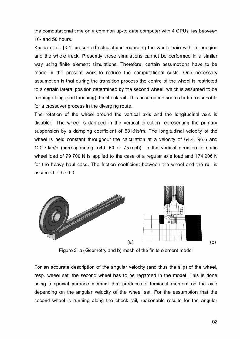
52
the computational time on a common up-to date computer with 4 CPUs lies between
10- and 50 hours.
Kassa et al. [3,4] presented calculations regarding the whole train with its boogies
and the whole track. Presently these simulations cannot be performed in a similar
way using finite element simulations. Therefore, certain assumptions have to be
made in the present work to reduce the computational costs. One necessary
assumption is that during the transition process the centre of the wheel is restricted
to a certain lateral position determined by the second wheel, which is assumed to be
running along (and touching) the check rail. This assumption seems to be reasonable
for a crossover process in the diverging route.
The rotation of the wheel around the vertical axis and the longitudinal axis is
disabled. The wheel is damped in the vertical direction representing the primary
suspension by a damping coefficient of 53 kNs/m. The longitudinal velocity of the
wheel is held constant throughout the calculation at a velocity of 64.4, 96.6 and
120.7 km/h (corresponding to40, 60 or 75 mph). In the vertical direction, a static
wheel load of 79 700 N is applied to the case of a regular axle load and 174 906 N
for the heavy haul case. The friction coefficient between the wheel and the rail is
assumed to be 0.3.
(a) (b)
Figure 2 a) Geometry and b) mesh of the finite element model
For an accurate description of the angular velocity (and thus the slip) of the wheel,
resp. wheel set, the second wheel has to be regarded in the model. This is done
using a special purpose element that produces a torsional moment on the axle
depending on the angular velocity of the wheel set. For the assumption that the
second wheel is running along the check rail, reasonable results for the angular
53
velocity of the wheel set are obtained. Details about this special purpose element are
described by the authors in [7].
The three-metre part of the crossing possesses a total mass of 680 kg. The material
is modelled with either elastic or elastic-plastic material behaviour. The mass of the
wheel is set to 1025 kg in the case of the regular axle load and 1500 kg in the heavy
haul case, respectively. The wheel is modelled with the elastic material behaviour of
steel. For the crossing materials models with different material descriptions are used:
a) the same elastic behaviour as for the wheel, b) elastic-plastic material behaviour of
non-pre-hardened Manganese steel (Mn13) and c) elastic-plastic material behaviour
of a maraging steel (Marage). The elastic constants and the yield stresses of the
used materials are given in Table 1. Since it is intended to compare very different but
commonly used crossing materials, Manganese steel is chosen that shows with
200 MPa a very low yield stress whereas the maraging steel exhibits with 1700 MPa
a very high yield stress. The plastic curves shown in Figure 3 illustrate the different
hardening behaviour of the two steels. A kinematic hardening model is used to
describe the material behaviour.
In the work presented in [7] the model uses rigid bedding of the crossing. So both the
support by the pad/sleeper/ground as well as the bending of the crossing between
the sleepers is neglected. For a more realistic bedding an activated mass, a spring
constant and a damping constant have to be regarded. For the sake of simplicity the
complex bedding system with a changing stiffness along the length of the crossing is
reduced to a single element of a spring and a damper in a parallel setup. The whole
bottom of the crossing is connected rigidly and supported by this spring-damper
element. The spring constant of the bedding is set to 90 kN/mm, the damping
constant to 250 Ns/mm and the spring supported mass amounts to 680 kg.
Table 1 The material parameters used in the model
Property Wheel (elastic) Manganese
steel (Mn13)
Maraging steel
(Marage)
Young’s modulus [GPa] 210 201 189
Poisson ratio 0.3 0.3 0.3
Density [kg/m3] 7800 7800 7800
Yield stress [MPa] - 200 1700

54
The model can describe the full cyclic elastic-plastic material behaviour of the
crossing. The plastic deformation strongly affects the contact stresses. In this work,
different load cases (axle loads, velocities and directions of passing) with elastic
crossing material are compared in terms of their arising stresses that can lead to
plastic deformation. From the von Mises stresses of this elastic calculation, it can be
predicted whether certain materials would plastically deform under this load.
In a separate model with elastic-plastic representation of the crossing material, the
plastic strains are calculated for one load cycle and two materials Mn13 and Marage.
Figure 3 Plastic curves for the two used materials Manganese steel (Mn13) and maraging steel
(Marage).
3 Results and Discussion
3.1 Dynamic results for one case of loading (forces, velocities, displacements) with elastic material
In Figure 4a, the vertical contact forces between the wheel and the wing rail and the
crossing nose are plotted. The sketch of a crossing below the diagram, having the
same length scale as the abscissa, allows to identify the wheel position on the
crossing.
At the start of the calculation, the wheel is placed on the wing rail at a wheel position
of 0 m. Then the wheel moves from left to right corresponding to a facing move. In a
dynamic calculation the placing of the wheel leads to oscillations especially of the
vertical contact force, see Figure 4a. These oscillations are visible from the start of
the calculations at wheel position 0 metres until a longitudinal wheel position of about
0.2 metres is reached. After 0.2 metres of rolling these start oscillations are
significantly damped. At about 0.2 metres the wing rail starts to deviate from the
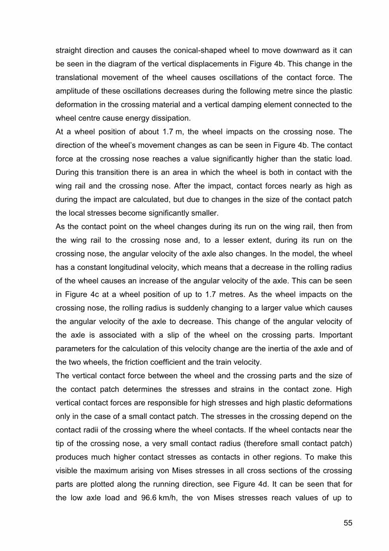
55
straight direction and causes the conical-shaped wheel to move downward as it can
be seen in the diagram of the vertical displacements in Figure 4b. This change in the
translational movement of the wheel causes oscillations of the contact force. The
amplitude of these oscillations decreases during the following metre since the plastic
deformation in the crossing material and a vertical damping element connected to the
wheel centre cause energy dissipation.
At a wheel position of about 1.7 m, the wheel impacts on the crossing nose. The
direction of the wheel’s movement changes as can be seen in Figure 4b. The contact
force at the crossing nose reaches a value significantly higher than the static load.
During this transition there is an area in which the wheel is both in contact with the
wing rail and the crossing nose. After the impact, contact forces nearly as high as
during the impact are calculated, but due to changes in the size of the contact patch
the local stresses become significantly smaller.
As the contact point on the wheel changes during its run on the wing rail, then from
the wing rail to the crossing nose and, to a lesser extent, during its run on the
crossing nose, the angular velocity of the axle also changes. In the model, the wheel
has a constant longitudinal velocity, which means that a decrease in the rolling radius
of the wheel causes an increase of the angular velocity of the axle. This can be seen
in Figure 4c at a wheel position of up to 1.7 metres. As the wheel impacts on the
crossing nose, the rolling radius is suddenly changing to a larger value which causes
the angular velocity of the axle to decrease. This change of the angular velocity of
the axle is associated with a slip of the wheel on the crossing parts. Important
parameters for the calculation of this velocity change are the inertia of the axle and of
the two wheels, the friction coefficient and the train velocity.
The vertical contact force between the wheel and the crossing parts and the size of
the contact patch determines the stresses and strains in the contact zone. High
vertical contact forces are responsible for high stresses and high plastic deformations
only in the case of a small contact patch. The stresses in the crossing depend on the
contact radii of the crossing where the wheel contacts. If the wheel contacts near the
tip of the crossing nose, a very small contact radius (therefore small contact patch)
produces much higher contact stresses as contacts in other regions. To make this
visible the maximum arising von Mises stresses in all cross sections of the crossing
parts are plotted along the running direction, see Figure 4d. It can be seen that for
the low axle load and 96.6 km/h, the von Mises stresses reach values of up to
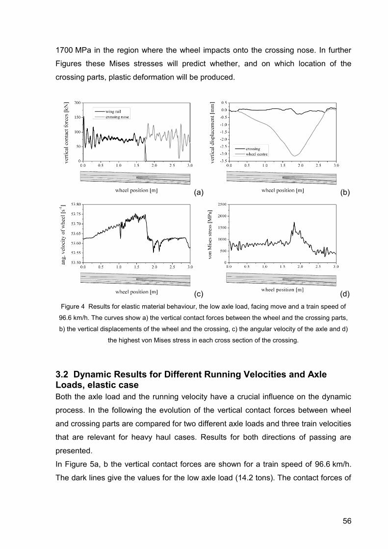
56
1700 MPa in the region where the wheel impacts onto the crossing nose. In further
Figures these Mises stresses will predict whether, and on which location of the
crossing parts, plastic deformation will be produced.
(a) (b)
(c) (d)
Figure 4 Results for elastic material behaviour, the low axle load, facing move and a train speed of
96.6 km/h. The curves show a) the vertical contact forces between the wheel and the crossing parts,
b) the vertical displacements of the wheel and the crossing, c) the angular velocity of the axle and d)
the highest von Mises stress in each cross section of the crossing.
3.2 Dynamic Results for Different Running Velocities and Axle Loads, elastic case
Both the axle load and the running velocity have a crucial influence on the dynamic
process. In the following the evolution of the vertical contact forces between wheel
and crossing parts are compared for two different axle loads and three train velocities
that are relevant for heavy haul cases. Results for both directions of passing are
presented.
In Figure 5a, b the vertical contact forces are shown for a train speed of 96.6 km/h.
The dark lines give the values for the low axle load (14.2 tons). The contact forces of

57
the heavy haul case with an axle load of 32.4 tons are plotted light gray. The dashed
horizontal lines represent the corresponding static loads of these two cases.
The impact of the wheel on the crossing nose (facing move) can be seen in figure 5a,
where the contact force has a peak at a wheel position of about 1.6 metres. The
whole development of the contact forces looks similar for the two axle loads;
however, their mean values are different. Due to the higher static load, the heavy
haul case shows a longer transition area. In the trailing move, the wheel impacts on
the wing rail and causes a peak in the contact forces on the wing rail, see figure 5b.
In the following, all maximum values of the contact force evolution during the
simulated 12 cases are compared. The results are shown for two axial load cases
(14.2 and 32.4 metric tons) and three assumed/calculated velocities of 64.4, 96.6 and
120.7 km/h.
(a) (b)
Figure 5 Contact forces between the wheel and the crossing parts for elastic crossing material at a
train speed of 96.6 km/h. The results are shown for two axle loads. Transition in a) facing move and
b) trailing move.
In Figure 6a the maximum vertical contact forces at the impact are shown. For
comparison of the different axle loads, also the dynamic factor of the impact is
presented in figure 6b. The dynamic factor is defined as the maximum arising contact
force divided by the static load.
Initially, as one would expect intuitively, the vertical contact forces increase with
increasing train speed as can be seen in Figure 6a,b. For the case of the low axle
load and the facing move, however, there is a slight decrease in the contact forces
towards higher velocities. This illustrates the complexity of the process, in which the
wheel due to its vertical oscillations might approach the crossing nose in a way that

58
produces less contact forces at a higher velocity. In all cases the dynamic factor
reaches values between 1.2 and 1.7.
(a) (b)
Figure 6 Comparison between the three velocities, two passing directions and the two axle loads. The
curves show a) peaks of the contact forces at the impact and b) dynamic factors of this impact for
elastic crossing material.
3.3 Stress Results for Different Running Velocities and Axle Loads
The development of the vertical contact forces characterizes the dynamic process.
The highest values of stress or strain in the crossing parts are caused by high
contact forces in a combination with narrow contact patches (e.g. at the tip of the
crossing nose).
For the evaluation of the material response, von Mises stresses are a better indicator
than the vertical contact forces. In figure 7, the development of the von Mises stress
along the crossing parts is shown for 96.6 km/h using an elastic crossing material.
The development of the von Mises stress during the facing move (Figure 7a) shows a
clear difference in its level for the two axle loads. For the low axle load, a maximum
von Mises stress of 1740 MPa is reached, whereas for the high axle load the
maximum amounts to 2320 MPa. Note that up to this point the material behaviour is
assumed purely elastic, thus overestimating the arising stresses. On the diverging
wing rail (wheel position of 0.2 to 1.7), a von Mises stress of 700 MPa (low axle load)
or 1200 MPa (high axle load) arise. After the impact of the wheel on the crossing
nose, the contact radius of the crossing increases and thus the stresses decrease.
Results of the von Mises stresses for the trailing move are shown in Figure 7b. The
results are similar to the ones for the facing move, with the difference that lower
maxima of the von Mises stresses are reached because the wheel does not impact

59
onto the narrow part of the crossing nose with its small contact radius. The von Mises
stresses amount to 1370 MPa for the low and 2080 MPa for the high axle load.
The maximum of the von Mises stress is located always at the tip of the crossing
nose, even if the wheel passes the crossing in the trailing move and impacts on the
wing rail. This is due to the small radius of the tip of the crossing nose.
If the von Mises stress exceeds the initial yield stress of the crossing material, plastic
strain occurs.
(a) (b)
Figure 7 Highest von Mises stress at a train speed of 96.6 km/h. Results for both axle loads.
Transition in a) facing move and b) trailing move. The yield stresses of crossing materials are
indicated by dashed lines.
A direct comparison of the highest von Mises stresses for the different moves, train
speeds and axle loads is shown in Figure 8. In addition, the yield stresses for the
Manganese steel (Mn13) and the maraging steel (Marage) are indicated by
horizontal dashed lines.
There is a clear tendency to higher von Mises stresses with increasing train speed
which is more pronounced for the facing move. The maximum von Mises stresses
are always detected in the crossing nose. They are higher for the facing move in
which the wheel impacts on the crossing nose. For the low axle load, the maximum
von Mises stress amounts to about 1400 MPa and increases only slightly with the
train speed for the case of the trailing move. For the low axle load and facing move,
the von Mises stress reaches up to 1590 MPa at 64.4 km/h and increases to
1830 MPa at 120.7 km/h. The levels of the von Mises stresses are generally higher
for the high axle load. For the trailing move they are about 2100 MPa and in the
facing move they increase from 2110 MPa at 64.4 km/h to 2360 MPa at 120.7 km/h.
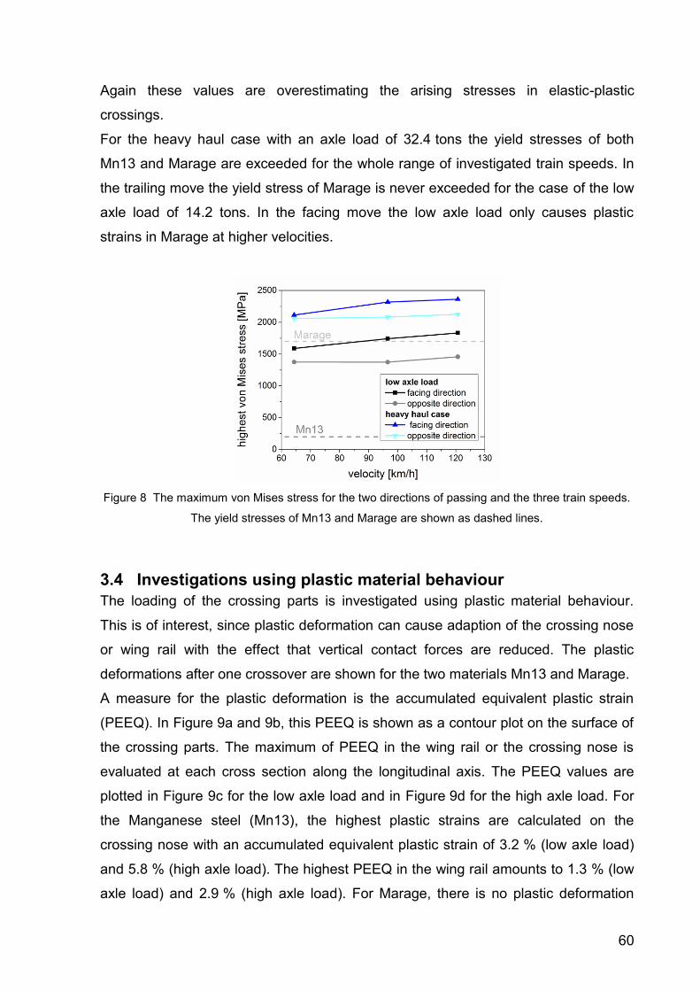
60
Again these values are overestimating the arising stresses in elastic-plastic
crossings.
For the heavy haul case with an axle load of 32.4 tons the yield stresses of both
Mn13 and Marage are exceeded for the whole range of investigated train speeds. In
the trailing move the yield stress of Marage is never exceeded for the case of the low
axle load of 14.2 tons. In the facing move the low axle load only causes plastic
strains in Marage at higher velocities.
Figure 8 The maximum von Mises stress for the two directions of passing and the three train speeds.
The yield stresses of Mn13 and Marage are shown as dashed lines.
3.4 Investigations using plastic material behaviour
The loading of the crossing parts is investigated using plastic material behaviour.
This is of interest, since plastic deformation can cause adaption of the crossing nose
or wing rail with the effect that vertical contact forces are reduced. The plastic
deformations after one crossover are shown for the two materials Mn13 and Marage.
A measure for the plastic deformation is the accumulated equivalent plastic strain
(PEEQ). In Figure 9a and 9b, this PEEQ is shown as a contour plot on the surface of
the crossing parts. The maximum of PEEQ in the wing rail or the crossing nose is
evaluated at each cross section along the longitudinal axis. The PEEQ values are
plotted in Figure 9c for the low axle load and in Figure 9d for the high axle load. For
the Manganese steel (Mn13), the highest plastic strains are calculated on the
crossing nose with an accumulated equivalent plastic strain of 3.2 % (low axle load)
and 5.8 % (high axle load). The highest PEEQ in the wing rail amounts to 1.3 % (low
axle load) and 2.9 % (high axle load). For Marage, there is no plastic deformation
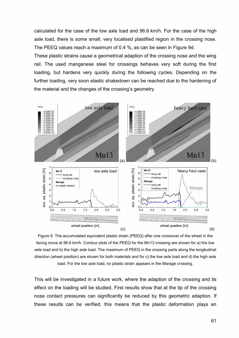
61
calculated for the case of the low axle load and 96.6 km/h. For the case of the high
axle load, there is some small, very localised plastified region in the crossing nose.
The PEEQ values reach a maximum of 0.4 %, as can be seen in Figure 9d.
These plastic strains cause a geometrical adaption of the crossing nose and the wing
rail. The used manganese steel for crossings behaves very soft during the first
loading, but hardens very quickly during the following cycles. Depending on the
further loading, very soon elastic shakedown can be reached due to the hardening of
the material and the changes of the crossing’s geometry.
(a) (b)
(c) (d)
Figure 9 The accumulated equivalent plastic strain (PEEQ) after one crossover of the wheel in the
facing move at 96.6 km/h. Contour plots of the PEEQ for the Mn13 crossing are shown for a) the low
axle load and b) the high axle load. The maximum of PEEQ in the crossing parts along the longitudinal
direction (wheel position) are shown for both materials and for c) the low axle load and d) the high axle
load. For the low axle load, no plastic strain appears in the Marage crossing.
This will be investigated in a future work, where the adaption of the crossing and its
effect on the loading will be studied. First results show that at the tip of the crossing
nose contact pressures can significantly be reduced by this geometric adaption. If
these results can be verified, this means that the plastic deformation plays an

62
important role in the development of wear and damage in the track. The calculated
plastic strains shown in Figure 9 indicate a positive effect on the performance of the
crossing (due to the geometric adaption).
3 Conclusions
A dynamic finite element model is developed for the crossing part of a turnout. Using
this model, the heavy haul case is investigated and compared to a regular axle load.
The model calculates the impact of the wheel on the crossing nose (facing move) or
the wing rail (trailing move), leading to dynamic contact forces which cause high
stresses and, depending on the material, plastic deformation. The results show that
also in cases with moderate dynamic contact forces high stresses are reached in the
crossing nose. During the trailing move, the maximum stresses still occur in the
crossing nose despite the fact that the impact occurs on the wing rail.
It is shown that the vertical contact forces during the impact of the wheel on the
crossing nose generally increase with higher running velocities of the train. For the
heavy haul case this effect is more distinctive than for the low axle load. The forces,
however, increase by less than 20 % in the investigated velocity range.
By evaluating the von Mises stress in the crossing parts of an elastic calculation, a
prediction whether the crossing will plastically deform can be made. It is shown that
for the very soft Manganese steel the crossing plastically deforms in all investigated
cases of velocities and axle loads. For hard maraging steel it is shown that for the
high axle load there is some plastic deformation and for the low axle load very little
(only in the facing move and at 120.7 km/h) or none. Hard materials such as
maraging steel crossings can show some advantages at higher loads when some
kind of plastic deformation can take place. This plastic adaption of the crossing can
reduce the contact stresses and thus the driving force for wear and RCF. The plastic
adaption of maraging steel is much less pronounced in applications with low axle
load.
Acknowledgements
Financial support by the Austrian Federal Government (in particular from the
Bundesministerium für Verkehr, Innovation und Technologie and the
Bundesministerium für Wirtschaft und Arbeit) and the Styrian Provincial Government,
63
represented by Österreichische Forschungsförderungsgesellschaft mbH and by
Steirische Wirtschaftsförderungsgesellschaft mbH, within the research activities of
the K2 Competence Centre on “Integrated Research in Materials, Processing and
Product Engineering”, operated by the Materials Center Leoben Forschung GmbH in
the framework of the Austrian COMET Competence Centre Programme, is gratefully
acknowledged.
References
[1] Knothe, K.L. and Grassie, S.L. Modelling of Railway Track and Vehicle/Track
Interaction at High Frequencies. Vehicle System Dynamics, 1993, 22(3-4), 209-
262.
[2] Kassa, E. Dynamic train-turnout interaction: mathematical modelling, numerical
simulation and field testing. PhD Thesis 2007, Chalmers University of
Technology, Gothenburg, Sweden.
[3] Kassa, E. and Nielsen, J.C.O. Stochastic analysis of dynamic interaction
between train and railway turnout. Vehicle System Dynamics, 2008, 46(5), 429-
449.
[4] Kassa, E. and Nielsen, J.C.O. Dynamic train-turnout interaction in an extended
frequency range using a detailed model of track dynamics. Journal of Sound
and Vibration, 2009, 320(4-5), 893-914.
[5] Johansson, A., Paulsson, B., Ekh, M., Nielsen, J.C.O., Ander, M.K.A.,
Brouzoulis, J. and Kassa, E. Simulation of wheel/rail contact and damage in
switches & crossings. Wear, 2010, 271(1-2), 472-481.
[6] Nicklisch, D., Kassa, E., Nielsen, J., Ekh, M. and Iwnicki, S. Geometry and
stiffness optimization for switches and crossings, and simulation of material
degradation. Proc. IMechE, Part F: Journal of Rail and Rapid Transit, 2010,
224(4), 279-292.
[7] Bruni, S., Anastasopoulos, I., Alfi, S., Van Leuven, A. and Gazetas, G. Effects
of train impacts on urban turnouts: Modelling and validation through
measurements. Journal of Sound and Vibration, 2009, 324(3-5), 666-689.
[8] Wiest, M. Modeling of wheel-rail/crossing interactions. PhD Thesis 2007,
University of Leoben, Austria.

64
[9] Wiest, M., Kassa, E., Daves, W., Nielsen, J.C.O. and Ossberger, H.
Assessment of methods for calculating contact pressure in wheel-rail/switch
contact. Wear, 2008, 265(9-10), 1439-1445.
[10] Pletz, M., Daves, W. and Ossberger, H. A Dynamical Wheel Set: Crossing
Model Regarding Impact, Sliding and Deformation. 8th International Conference
on Contact Mechanics and Wear of Rail/Wheel Systems, Florence, Italy, 2009,
pp. 801-809.
[11] Pletz, M., Daves, W. and Ossberger, H. Dynamic Finite Element Model of a
Wheel Passing a Crossing Nose. Tenth International Conference on
Computational Structures Technology, Valencia, Spain, 2010, on-line.
[12] Wiest, M., Daves, W., Fischer, F.D. and Ossberger, H. Deformation and
damage of a crossing nose due to wheel passages. Wear, 2008, 265(9-10),
1431-1438.

65
Paper C
The Plastic Adaption of Railway Crossings due to
Dynamic Contact Loading – an Explicit Finite
Element Study
M. Pletz
W. Daves
H. Ossberger
To be submitted

66
The Plastic Adaption of Railway Crossings due to
Dynamic Contact Loading – an Explicit Finite
Element Study
M. Pletz1,2, W. Daves1,2, S. Eck2, H. Ossberger3
1Materials Center Leoben Forschung GmbH, Leoben, Austria
2Institute of Mechanics, Montanuniversität Leoben, Leoben, Austria
3VAE GmbH, Zeltweg, Austria
Abstract
A model for the description of the plastic adaption of the crossing nose of a turnout
and its effect on the contact forces and contact stresses is presented. A wheel
initially running on the wing rail and impacting on the crossing nose has been
modelled. In one case, the impact position of the wheel on the crossing nose was
varied to account for changing loading situations in the track. A comparison with a
non-realistic situation of a wheel impacting always at the same position of the nose
was performed to identify the influence of the cyclic material response.
The main results of the model are the contact forces between the wheel and the
crossing nose, the plastic strains, the change of the crossing profile, and the contact
pressure. The evolution of these values has been described for the first 20 cycles. It
has been found that a significant decrease of the contact pressure is caused by
plastic adaption of the crossing material.
Three different cyclic material descriptions (a Hadfield type austenitic steel, a grain
refined construction steel and a tempered hot working tool steel) have been used in
the model. The parameters of the corresponding cyclic elastic-plastic material models
have been derived from monotonic tensile tests as well as low cycle fatigue tests.
1 Introduction
Turnouts are an important part of the railway track structure and consist of switch and
crossing panels. A typical crossing is shown in Figure 1, consisting of two wing rails
and the crossing nose. At the crossing panel, there is a discontinuity in the track. This
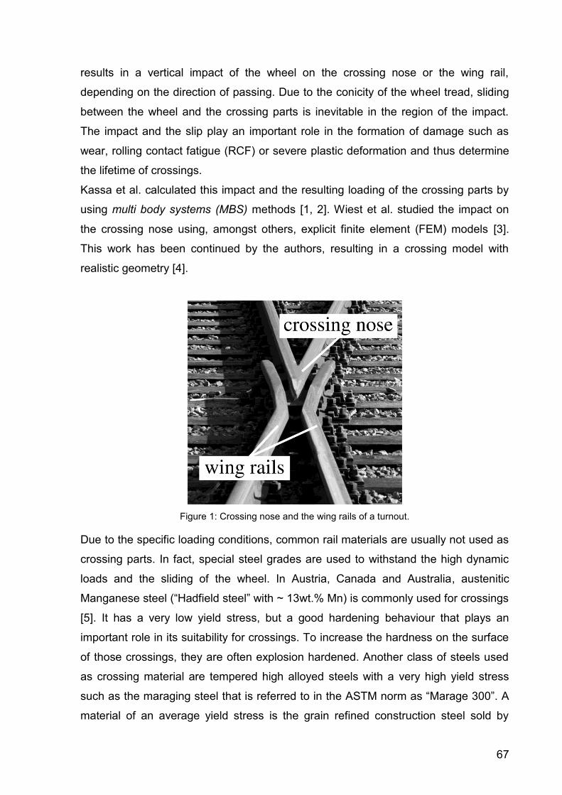
67
results in a vertical impact of the wheel on the crossing nose or the wing rail,
depending on the direction of passing. Due to the conicity of the wheel tread, sliding
between the wheel and the crossing parts is inevitable in the region of the impact.
The impact and the slip play an important role in the formation of damage such as
wear, rolling contact fatigue (RCF) or severe plastic deformation and thus determine
the lifetime of crossings.
Kassa et al. calculated this impact and the resulting loading of the crossing parts by
using multi body systems (MBS) methods [1, 2]. Wiest et al. studied the impact on
the crossing nose using, amongst others, explicit finite element (FEM) models [3].
This work has been continued by the authors, resulting in a crossing model with
realistic geometry [4].
Figure 1: Crossing nose and the wing rails of a turnout.
Due to the specific loading conditions, common rail materials are usually not used as
crossing parts. In fact, special steel grades are used to withstand the high dynamic
loads and the sliding of the wheel. In Austria, Canada and Australia, austenitic
Manganese steel (“Hadfield steel” with ~ 13wt.% Mn) is commonly used for crossings
[5]. It has a very low yield stress, but a good hardening behaviour that plays an
important role in its suitability for crossings. To increase the hardness on the surface
of those crossings, they are often explosion hardened. Another class of steels used
as crossing material are tempered high alloyed steels with a very high yield stress
such as the maraging steel that is referred to in the ASTM norm as “Marage 300”. A
material of an average yield stress is the grain refined construction steel sold by
68
SSAB under the brand name “Hardox 400”, which is used for tramway crossings and
all kinds of applications where wear-resistance is of importance [6].
Depending on the mechanical behaviour of the crossing material, it often plastically
deforms in the region where the wheel impacts on it. With this deformation the
crossing nose tends to adapt to the geometry of the wheel. For high cycle numbers
wear can have a similar effect due to material loss and resulting geometrical
adaption. In rails adaption is probably not an ideal behaviour since conformal contact
causes very high slip and results in wear or RCF. In crossing noses, however, the
high contact pressure of the impact can be strongly reduced by this adaption, thus
lowering wear and RCF.
The adaption of the crossing nose to the loading was investigated first by Wiest et al.
with a FE model using simplified geometry and loading conditions. A clear decrease
in the contact pressure and slight decrease of the dynamic load with proceeding
plastic adaption has been found and published in [7]. Johansson et al. [8] have
developed a model that can predict profile changes due to plastic deformation and
wear. With this model a comparison with observed profile changes in the track has
been conducted by Nicklish et al. [9]. It is based on a global MBS model, combined
with a three-dimensional micro-model for the plastic contact pressure distributions, a
two-dimensional model for calculating the plastic profile change and the FASTSIM
[10] algorithm to predict wear. Up to 200 000 cycles were calculated, and a good
agreement between profile measurements and simulations was reached. This
methodology, however, needs some calibration and the use of several interfaces
between different methods (MBS, FEM and FASTSIM).
In this work a dynamic finite element model is used to describe the plastic adaption of
the crossing in the first 20 cycles. The contact situation and the elastic-plastic
deformation of wheel and crossing are calculated in a single model. The model
allows to study the effect of the plastic adaption on the dynamic contact forces and
the contact stresses. As the material of the crossing plays an important role in this
adaption process, the three materials Hadfield steel (in the following referred to as
Mn13), Hardox 400 (Hardox) and Marage 300 (Marage) are used in the calculations.
Elastic-plastic material models for these materials have been derived from
mechanical tests. The FE model uses two types of loading: The wheel is impacting
always at (a) the same position or (b) varying position on the crossing. The effect of
these types of loading on the crossings adaption is described.

69
2 Methods
2.2 Mechanical tests
For the determination of the material parameters of the investigated crossing
materials, monotonic tensile tests and low cycle fatigue (LCF) tests were conducted.
The cylindrical specimens had an hourglass shape with a gauge length of 10 mm and
a 10 mm diameter within this gauge length. The surface of the specimens was
polished. In the monotonic tensile tests, the strain rate was 0.01 s-1; strain rate
dependency was not investigated. Strain-controlled LCF tests have been performed
with two total strain amplitudes per material, as given in Table 1. The strain was
applied with a saw-tooth wave shape with zero mean strain and a strain ratio R of -1.
The first half cycle of loading was in compression and all experiments were
conducted at room temperature.
Table 1: Strain amplitudes used in the LCF tests.
Strain amplitudes a of the
LCF test
Marage 1.1 % 1.5 %
Hardox 0.9 % 1.3 %
Mn13 0.9 % 1.1 %
2.2 Modelling
2.2.1 The crossing model
In previous work [4, 11, 12] a model for the crossing has been developed with the
finite element code ABAQUS/Explicit [13]. In this model, a three metre part of the
crossing is modelled, in which the wheel changes from the wing rail to the crossing
nose. The mesh of the model can be seen in Figure 2. For the first passing wheel the
influence of the train speed, the axle load, the wheel profile, the direction of passing
and the crossing profile on the process can be investigated. The calculated results
include the maximum vertical contact forces, the wheel movement, the longitudinal
position of impact on the crossing nose, the contact pressure, the slip and the plastic
strains. The following assumptions concerning the boundary conditions have been
made: The longitudinal velocity of the wheel is held constant, there is no steering of

70
the bogie and the wheel has a constant lateral position. Details about the model
assumptions and results are given in [4].
With this crossing model that contains about 250 000 elements causing calculation
times of 8h on an up-to-date four-core computer cyclic studies would be very time-
consuming. The crossing model has elements with an edge-length of 3 mm in the
contacting areas, which is sufficient for a good description of the dynamics and a
rough but usually sufficiently accurate description of contact pressure, slip and plastic
deformation. However, for a more detailed study of the adaption of the crossing nose
(in terms of stresses and strains) the calculation times have to be reduced and the
elements in the crossing nose have to be refined.
Figure 2: The crossing model with the wheel, two wing rails and the crossing nose. A total length of 3
metres is modelled.
2.2.2 The impact model
In the new impact model, only the 0.5 metre part of the crossing nose where the
wheel impacts, has been modelled. The case of the facing move (wheel initially
running on the wing rail and impacting onto the crossing nose) is investigated. The
investigations consider a new wheel profile, a train speed of 160 km/h and an axle
load of 14.2 tons. In Figure 3, the results of the crossing model are shown for this
case. The corresponding region of the impact model (1.7 to 2.2 metres) is indicated
by two lines. Within this distance, it can be seen that the wheel changes its vertical
movement and the angular velocity of the wheel decreases. The results (e.g. the
calculated accumulated plastic strains shown in Figure 3c) show that the impact of
the wheel on the crossing nose is associated with high plastic deformations. The
initial vertical wheel and crossing position and the wheel velocity, see also Figure 3,
are subsequently used as initial conditions in the impact model.
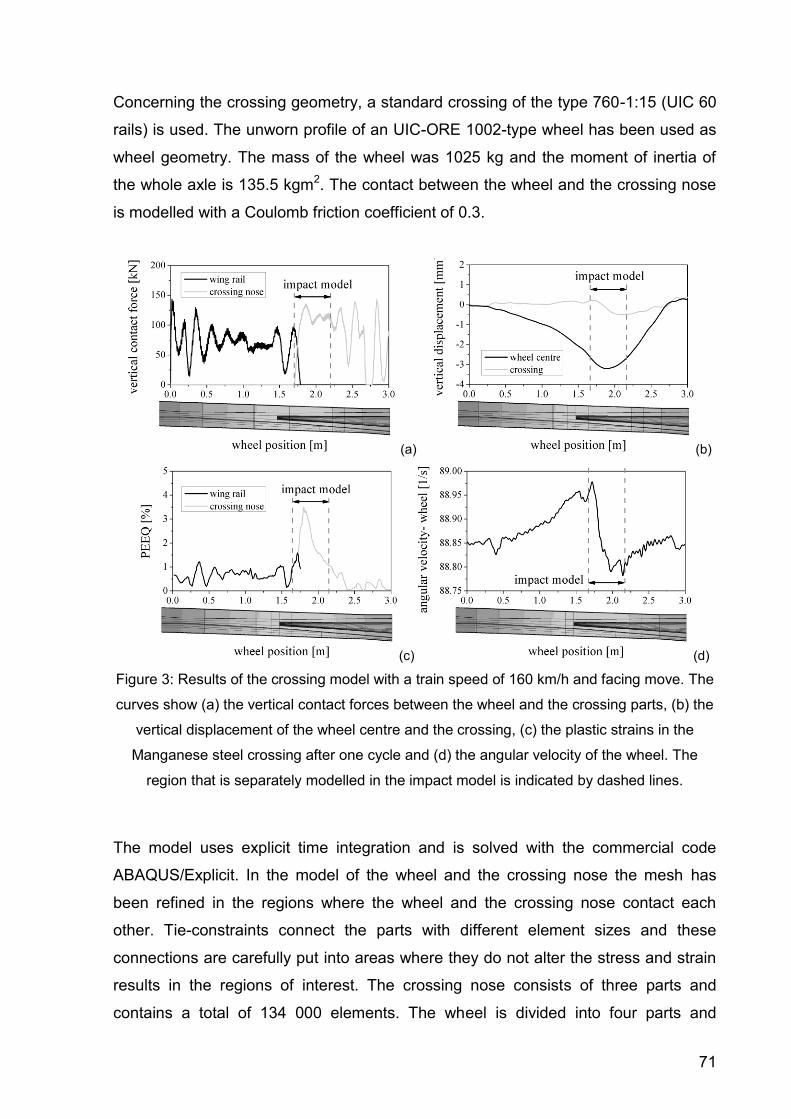
71
Concerning the crossing geometry, a standard crossing of the type 760-1:15 (UIC 60
rails) is used. The unworn profile of an UIC-ORE 1002-type wheel has been used as
wheel geometry. The mass of the wheel was 1025 kg and the moment of inertia of
the whole axle is 135.5 kgm2. The contact between the wheel and the crossing nose
is modelled with a Coulomb friction coefficient of 0.3.
(a) (b)
(c) (d)
Figure 3: Results of the crossing model with a train speed of 160 km/h and facing move. The
curves show (a) the vertical contact forces between the wheel and the crossing parts, (b) the
vertical displacement of the wheel centre and the crossing, (c) the plastic strains in the
Manganese steel crossing after one cycle and (d) the angular velocity of the wheel. The
region that is separately modelled in the impact model is indicated by dashed lines.
The model uses explicit time integration and is solved with the commercial code
ABAQUS/Explicit. In the model of the wheel and the crossing nose the mesh has
been refined in the regions where the wheel and the crossing nose contact each
other. Tie-constraints connect the parts with different element sizes and these
connections are carefully put into areas where they do not alter the stress and strain
results in the regions of interest. The crossing nose consists of three parts and
contains a total of 134 000 elements. The wheel is divided into four parts and
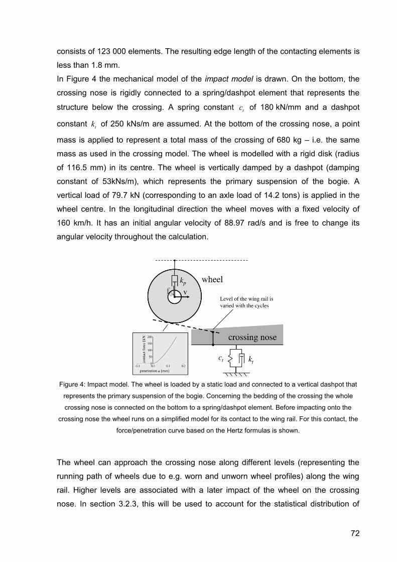
72
consists of 123 000 elements. The resulting edge length of the contacting elements is
less than 1.8 mm.
In Figure 4 the mechanical model of the impact model is drawn. On the bottom, the
crossing nose is rigidly connected to a spring/dashpot element that represents the
structure below the crossing. A spring constant tc of 180 kN/mm and a dashpot
constant tk of 250 kNs/m are assumed. At the bottom of the crossing nose, a point
mass is applied to represent a total mass of the crossing of 680 kg – i.e. the same
mass as used in the crossing model. The wheel is modelled with a rigid disk (radius
of 116.5 mm) in its centre. The wheel is vertically damped by a dashpot (damping
constant of 53kNs/m), which represents the primary suspension of the bogie. A
vertical load of 79.7 kN (corresponding to an axle load of 14.2 tons) is applied in the
wheel centre. In the longitudinal direction the wheel moves with a fixed velocity of
160 km/h. It has an initial angular velocity of 88.97 rad/s and is free to change its
angular velocity throughout the calculation.
Figure 4: Impact model. The wheel is loaded by a static load and connected to a vertical dashpot that
represents the primary suspension of the bogie. Concerning the bedding of the crossing the whole
crossing nose is connected on the bottom to a spring/dashpot element. Before impacting onto the
crossing nose the wheel runs on a simplified model for its contact to the wing rail. For this contact, the
force/penetration curve based on the Hertz formulas is shown.
The wheel can approach the crossing nose along different levels (representing the
running path of wheels due to e.g. worn and unworn wheel profiles) along the wing
rail. Higher levels are associated with a later impact of the wheel on the crossing
nose. In section 3.2.3, this will be used to account for the statistical distribution of
73
wheel profiles, train speeds and axle loads. The vertical initial positions of the wheels
have been varied between 0 mm and 1.6 mm, resulting in varied longitudinal impact
positions between 0.05 m and 0.35 m.
To consider the influence of the second wheel on the angular velocity of the axle, a
frictional element is used that has been developed for the crossing model [4]. The
influence of the wing rail on the angular velocity of the wheel (the angular velocity
increase before the impact) determines the initial angular velocity. In the impact
model no further acceleration due to the wheel’s run along the wing rail is
considered.
To account for the contact of the wheel with the wing rail, the centre of the wheel is
vertically connected to a contact spring. It is assumed that the contact situation does
not change in the longitudinal direction. Using the Hertzian formulas [14], the contact
stiffness can be derived from the elastic constants of the material and the geometry
represented by the radii of the contacting bodies. For the wheel and wing rail, a
Young’s modulus of 210 GPa and a Poisson’s ratio of 0.3 is used. A wheel radius of
0.5 m is assumed while the radius in the lateral direction is infinite. For the wing rail,
the radius in the longitudinal direction is infinite and 40 mm in the lateral direction.
These values result in a penetration of the contacting bodies w of
3/28 2/3( ) 3.92 10N
w F Fm
(1)
Although the geometry of the contact changes slightly along the wing rail, this
formula is used for the whole distance. A constant inclination of the wing rail (angle of
0.223 degrees) is assumed, which defines the downward movement of the wheel
during the start of the calculation.
Initially, the spring of the crossing’s bedding and the contact spring are compressed
according to the vertical load on the wheel. Subsequently, the vertical load is applied
in the wheels centre, causing some oscillations of the contact force between the
wheel and the simplified wing rail. At the point where the wheel impacts onto the
crossing nose those oscillations have already faded away.
To start with, the calculations were carried out for different initial wheel positions and
an elastic material behaviour of the crossing only. Results of this elastic model are
shown in section 3.2.1. Subsequently, 21 cycles have been calculated with the
lowest (or first) vertical wheel position (0 mm) and for the three materials including
their plastic properties, see section 3.2.2. In another calculation, 21 wheels with 10
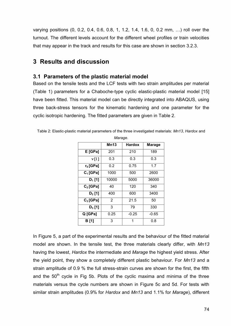
74
varying positions (0, 0.2, 0.4, 0.6, 0.8, 1, 1.2, 1.4, 1.6, 0, 0.2 mm, …) roll over the
turnout. The different levels account for the different wheel profiles or train velocities
that may appear in the track and results for this case are shown in section 3.2.3.
3 Results and discussion
3.1 Parameters of the plastic material model
Based on the tensile tests and the LCF tests with two strain amplitudes per material
(Table 1) parameters for a Chaboche-type cyclic elastic-plastic material model [15]
have been fitted. This material model can be directly integrated into ABAQUS, using
three back-stress tensors for the kinematic hardening and one parameter for the
cyclic isotropic hardening. The fitted parameters are given in Table 2.
Table 2: Elastic-plastic material parameters of the three investigated materials: Mn13, Hardox and
Marage.
Mn13 Hardox Marage
E [GPa] 201 210 189
0.3 0.3 0.3
r0 [GPa] 0.2 0.75 1.7
C1 [GPa] 1000 500 2600
D1 [1] 10000 5000 36000
C2 [GPa] 40 120 340
D2 [1] 400 600 3400
C3 [GPa] 2 21.5 50
D3 [1] 3 79 330
Q [GPa] 0.25 -0.25 -0.65
B [1] 3 1 0.8
In Figure 5, a part of the experimental results and the behaviour of the fitted material
model are shown. In the tensile test, the three materials clearly differ, with Mn13
having the lowest, Hardox the intermediate and Marage the highest yield stress. After
the yield point, they show a completely different plastic behaviour. For Mn13 and a
strain amplitude of 0.9 % the full stress-strain curves are shown for the first, the fifth
and the 50th cycle in Fig 5b. Plots of the cyclic maxima and minima of the three
materials versus the cycle numbers are shown in Figure 5c and 5d. For tests with
similar strain amplitudes (0.9% for Hardox and Mn13 and 1.1% for Marage), different

75
stress levels are obtained. Mn13 shows strong hardening whereas both Hardox and
Marage soften with proceeding cyclic loading. Generally, a good agreement between
the experiments and the fitted material model has been reached. The experimental
results show a slightly different material behaviour in tension and compression for all
materials, but this discrepancy is considered negligible and therefore not included in
the material model.
(a) (b)
(c) (d)
Figure 5: Measured (black curves) and fitted (grey curves) data for the three materials. The curves
show (a) the tensile tests for all materials, (b) the cyclic response of Mn13 with strain amplitude of
0.9 %, (c) the maximum cyclic stress for the lower stain amplitudes of the materials and (d) the
corresponding minimum of the cyclic stress.
3.2 Results of the impact model
3.2.1 Elastic results of the impact model
In Figure 6, the results of the model with elastic crossing material and initial vertical
wheel positions of 0, 0.4, 0.8, 1.2 and 1.6 mm are shown. The vertical contact forces
resulting from the impact are shown in Figure 6a. Note that the definition of the wheel
position differs from the crossing model shown in Figure 3. In the impact model, the
position of 0 metres corresponds to the tip of the crossing nose. It can be seen that
the impact produces forces that reach values of up to 210 kN, i.e. more than two

76
times the static load (79.7 kN). The impact of the wheel occurs farther in longitudinal
direction for the wheels with higher initial positions. The maximum contact forces are
slightly higher for the later impacts of the wheel. The vertical displacements of the
wheel centre are illustrated in Figure 6b. As the wheel initially runs on the wing rail, it
linearly lowers its position. After the impact oscillations of the vertical wheel
displacements can be seen. They correspond to the oscillations of the contact forces,
see Figure 6a.
The calculated contact areas of the contact patch between the wheel and the
crossing nose are shown in Figure 6c. The contact areas increase towards the end of
the crossing nose as the contact radius of the crossing nose increases. The contact
patch can reach a size of 150 mm2 corresponding to a circle with a diameter of 14
mm. The division of the vertical contact forces by the contact area results in the
average contact pressure plotted in Figure 6d.
(a) (b)
(c) (d)
Figure 6: The results of the impact model with elastic behaviour of the crossing. For the levels of 0,
0.4, 0.8, 1.2 and 1.6 mm, (a) the vertical contact force between wheel and crossing nose, (b) the
vertical displacement of the wheels centre, (c) the contact area and (d) the average contact pressure
are shown.

77
3.2.2 Loading by wheels impacting at the same position
The results for a series of 21 wheels impacting onto the crossing nose with initial
positions of 0 mm are plotted in Figure 7. The change in the vertical contact forces
due to consecutive impacts as well as the change in the average contact pressure
influenced by the ongoing plastic deformation is illustrated. The results for the three
materials Marage, Hardox and Mn13 are shown for the first, the 11th and the 21st
cycle.
Fig 7a,c,e shows the evolution of the vertical contact forces. With Marage as crossing
material, the calculations indicate nearly no change in the force results during the first
21 cycles. For Hardox the plastic deformation of the crossing causes a slight
increase of the contact forces during progressing impacts. For Mn13, the highest
contact forces are obtained further away from the tip of the crossing nose. Due to the
plastic deformation and thus geometric adaption the contact forces of the first cycle
are smaller than the forces of the calculations with elastic material response. At
higher load cycles, however, the vertical contact forces reach higher values than in
the case of the elastic calculations. This can be attributed to an excitation of
additional oscillations due to the development of a deep dent caused by impacts of
the wheel at the same position of the Mn13 crossing nose. At a wheel position of
about 0.35 m, the wheel nearly loses contact with the crossing nose. Concerning the
dynamic contact forces this adaption in the form of a dent of the Mn13 crossing is not
beneficial. However, this dent will only be produced as a result of the unrealistic case
of identical impacts meaning new wheels having exactly the same profile, same
running position, same running velocity and same load during the loading of a new
crossing nose.
The average contact pressure of the same position loading is shown in Figure 7b,d,f.
In contrast to the contact force an effect of the small plastic deformation in the case
of Marage crossings on the contact pressure is found. During the first cycle, the
contact pressure is nearly identical with the elastic case (maximum of 1488 MPa).
After 11 and 21 load cycles, however, some plastic deformation accumulates,
causing the highest average pressure to drop from 1437 MPa (first cycle) to
1136 MPa (11th cycle) and 1134 MPa (21st cycle). A similar effect can be seen in the
model with the Hardox crossing, where the plastic deformations are higher than the
ones for Marage and the average pressure drops from 1408 MPa (first cycle) to
1102 MPa (11th cycle) and 1069 MPa (21st cycle) during the impact. For Marage and

78
Hardox crossings the plastic deformation of the first load cycle mainly causes that
decrease of the average pressure. The following cycles contribute much less. The
manganese steel crossing shows a clear adaption and decrease of the average
contact pressure to 793 MPa during the impact of the first cycle. With the proceeding
plastic deformation and geometrical adaption the average pressure is further lowered
to 636 MPa in the 11th and 611 MPa in the 21st cycle despite the fact that the material
hardens. Due to the opposing effects of the geometric adaption of the crossing and
the hardening of the Mn13, the adaption process almost stops after a few cycles.
Thus, elastic shakedown is nearly reached.
The cause for the evolution of contact forces and the decrease of the average
contact pressure can be assigned to the change in the longitudinal and lateral
crossing profile. This is illustrated in Figure 8. The longitudinal profile change of the
crossing is shown in Figure 8a. The vertical position of the contact point initially rises
linearly towards the end of the crossing. After 20 wheels have impacted on the
crossing at the same position, some waviness of the crossing profile can be seen.
For Mn13, this adaption is very pronounced with a dent depth of 0.35 mm, whereas
for Hardox there is only a slight change (up to 0.07 mm dent depth) at the tip of the
crossing, and for Marage there is nearly no change. As the wheel has to follow the
deformed profile during the following impacts, additional oscillations are introduced
into the system. The slower and later impact for the Mn13 can be understood with
this picture, as well as the higher contact forces and the bouncing of the wheel after
the wheel has reached a position of 0.3 metres in the diagram, see Figure 7e.
In Figure 8b, the maxima of the accumulated equivalent plastic strain (PEEQ) are
shown for the three materials after the 20th load cycle. The Marage crossing shows
only little deformations with plastic strains of up to 0.74 %. For Hardox, the PEEQ
reaches values of up to 5.8 % and for Mn13 of up to 21.5 %. High plastic
deformations are obtained for the Mn13 crossing nearly over the whole modelled
length of the crossing nose. At a wheel position of 0.1 m, the Marage and Hardox
crossings show their highest PEEQ values. For Mn13, the highest PEEQ is reached
at a wheel position of 0.2 m.
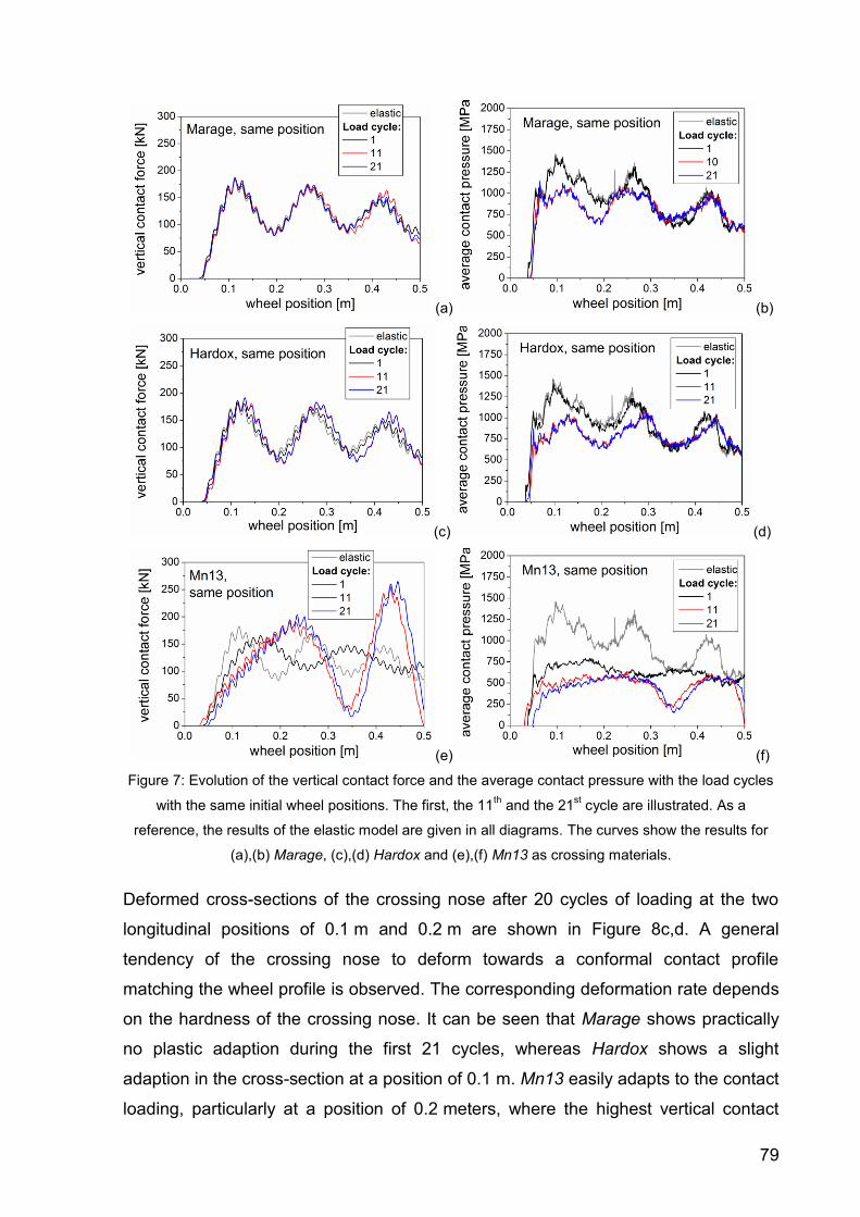
79
(a) (b)
(c) (d)
(e) (f)
Figure 7: Evolution of the vertical contact force and the average contact pressure with the load cycles
with the same initial wheel positions. The first, the 11th and the 21
st cycle are illustrated. As a
reference, the results of the elastic model are given in all diagrams. The curves show the results for
(a),(b) Marage, (c),(d) Hardox and (e),(f) Mn13 as crossing materials.
Deformed cross-sections of the crossing nose after 20 cycles of loading at the two
longitudinal positions of 0.1 m and 0.2 m are shown in Figure 8c,d. A general
tendency of the crossing nose to deform towards a conformal contact profile
matching the wheel profile is observed. The corresponding deformation rate depends
on the hardness of the crossing nose. It can be seen that Marage shows practically
no plastic adaption during the first 21 cycles, whereas Hardox shows a slight
adaption in the cross-section at a position of 0.1 m. Mn13 easily adapts to the contact
loading, particularly at a position of 0.2 meters, where the highest vertical contact
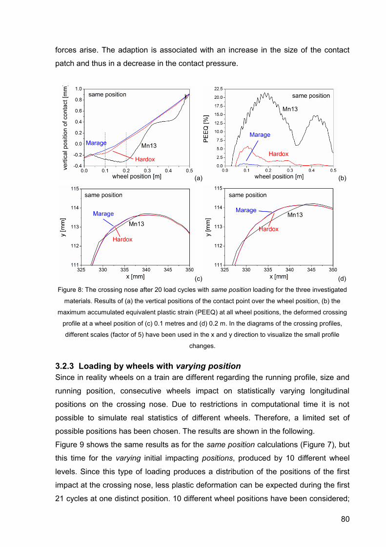
80
forces arise. The adaption is associated with an increase in the size of the contact
patch and thus in a decrease in the contact pressure.
(a) (b)
(c) (d)
Figure 8: The crossing nose after 20 load cycles with same position loading for the three investigated
materials. Results of (a) the vertical positions of the contact point over the wheel position, (b) the
maximum accumulated equivalent plastic strain (PEEQ) at all wheel positions, the deformed crossing
profile at a wheel position of (c) 0.1 metres and (d) 0.2 m. In the diagrams of the crossing profiles,
different scales (factor of 5) have been used in the x and y direction to visualize the small profile
changes.
3.2.3 Loading by wheels with varying position
Since in reality wheels on a train are different regarding the running profile, size and
running position, consecutive wheels impact on statistically varying longitudinal
positions on the crossing nose. Due to restrictions in computational time it is not
possible to simulate real statistics of different wheels. Therefore, a limited set of
possible positions has been chosen. The results are shown in the following.
Figure 9 shows the same results as for the same position calculations (Figure 7), but
this time for the varying initial impacting positions, produced by 10 different wheel
levels. Since this type of loading produces a distribution of the positions of the first
impact at the crossing nose, less plastic deformation can be expected during the first
21 cycles at one distinct position. 10 different wheel positions have been considered;
81
during the first, the 11th and the 21st cycle the wheel impacts at the same longitudinal
position (level of 0 mm), and therefore these cycles can be compared in the following
diagrams.
In Fig 9a,c,e, it can be seen that the highest forces of the first cycle are slightly lower
than the values of the elastic calculation. This is valid for all investigated materials.
For the subsequent loading of the crossing, however, the contact forces slightly
increase in the Marage and the Hardox simulations. For Mn13, the highest contact
forces are not necessarily obtained during the first impact but sometimes during the
following oscillations and a further position on the crossing. Compared to the
calculations with same position of the wheel, the contact forces are reduced
regarding the first impact and the following oscillations. This is a result of the plastic
deformation and an advantageous adaptation of the geometry of the crossing nose.
The average contact pressure is shown in Figure 9b,d,f. Similar to the model with the
same wheel position, the pressure decreases due to the plastic deformation mainly
caused by the first load cycle. Later on, only small changes are obtained. In the
Mn13 crossing, due to the heavy plastic deformation the contact pressure in the first
cycle is clearly lower (800 MPa) than in the elastic model. In the following load
cycles, the highest average pressure reaches values of about 640 MPa. For Hardox
and Marage, there is also a tendency of the average pressure to decrease with
advancing cycles. For the model with varying position loading, however, there are
some tolerances in the relative vertical position between rail and crossing. For
Marage, this causes the average pressure of the 21st cycle with 1334 MPa to be
higher than the 11th cycle with 1139 MPa because the wheel impacts earlier on the
crossing nose.
In Figure 10a, the vertical position of the centre of the contact patch – representing
the running level of the wheel - is shown after 20 wheels have passed (impacting at
different positions). It can be seen that for the two better adapting materials (Hardox,
and Mn13) a fairly uniform deformation and even shape of the crossing nose is
produced in longitudinal direction. For Mn13, this results in a decrease of the vertical
contact forces with progressing loadings. The accumulated equivalent plastic strains
(PEEQ) are more or less uniformly distributed along the crossing. The highest values
of the PEEQ after 20 cycles of loading are 0.5 % for Marage, 3 % for Hardox and
14.4 % for Mn13.
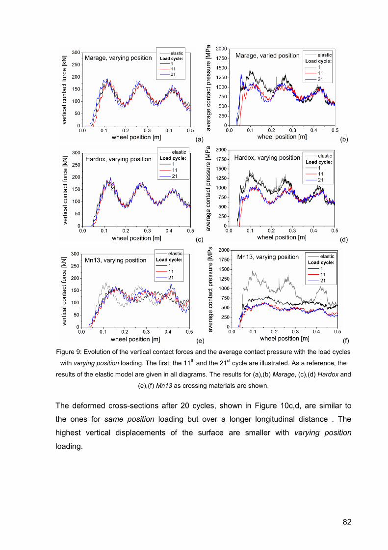
82
(a) (b)
(c) (d)
(e) (f)
Figure 9: Evolution of the vertical contact forces and the average contact pressure with the load cycles
with varying position loading. The first, the 11th and the 21
st cycle are illustrated. As a reference, the
results of the elastic model are given in all diagrams. The results for (a),(b) Marage, (c),(d) Hardox and
(e),(f) Mn13 as crossing materials are shown.
The deformed cross-sections after 20 cycles, shown in Figure 10c,d, are similar to
the ones for same position loading but over a longer longitudinal distance . The
highest vertical displacements of the surface are smaller with varying position
loading.

83
(a) (b)
(c) (d)
Figure 10: The crossing nose after 20 load cycles with varying position loading for the three
investigated materials. Results of (a) the vertical positions of the contact point over the wheel position,
(b) the maximum accumulated equivalent plastic strain (PEEQ) at all wheel positions, the deformed
crossing profile at a wheel position of (c) 0.1 metres and (d) 0.2 m. In the diagrams of the crossing
profiles, different scales (factor of 5) have been used in the x and y direction to visualize the small
profile changes.
3.3.4 The tendency of the crossing to form dents
In Figure 8a, the loading with same position causes waviness in the crossings
surface for Mn13 and a less pronounced one for Hardox. Different initial wheel
positions, on the other hand, show a more uniform deformation of the surface, see
Figure 10a. The wave formation in Mn13 crossings excites high contact forces and
subsequent oscillations, see Figure 7e. This unrealistic case increases the dynamic
loads, which in turn further increase those deformations.
The key factor for this wave formation is the uniformity of the loading. The more
uniform the wheel profiles, the train speeds, the bogies and the axle loads are, the
more the crossing tends to form waves. The exact role of the material behaviour in
these models will be the subject of further calculations. Waviness produced after
some cycles is favoured by materials with low yield stress. Whether harder materials
with cyclic softening behaviour tend, on a longer term, to form dents cannot be
clarified by the presented work due to the extensive amount of cycles (more than
84
1000) needed for this kind of investigation. It can be assumed that softening
materials tend to increase existing dents whereas hardening materials may have the
ability to smooth out dents if the loading position is not always the same.
3.3 Reduction of loads as result of the crossings geometrical adaption
From Figure 7 and Figure 9, it can already be seen that the average contact pressure
is reduced by the plastic deformation of the crossing nose.
In Figure 11, contour plots of the vertical stresses yy are shown at a wheel position
of 0.2 m for the 21st cycle of loading with varying wheel positions. To highlight the
effect of the plastic deformation on the stresses, the results of the elastic model are
shown, too.
In the elastic model, the vertical stress (and thus the contact pressure) reach a
minimum value of 2215 MPa (maximum contact pressure of 2215 MPa). At this wheel
position, the model with the Marage crossing shows with a maximum contact
pressure of 2212 MPa no significant decrease in the stresses. For Hardox, the
contour plot shows that the contact patch has increased in size and the highest
contact pressure is reduced to 1674 MPa. The Mn13 crossing adapts best and
reduces the maximum contact pressure to 935 MPa.
From these results it can be concluded that the crossing profile can in the case of
Mn13 easily approach the shape of the wheel profile in the contacting region. This
change of the contact radii causes a nearly conformal contact and the lateral size of
the contact patch increases. In the longitudinal direction the size of the contact patch
stays about the same. For similar vertical contact forces the contact pressure is thus
drastically reduced.
This lateral geometric adaption is determined by the plastic material behaviour of the
crossing nose. The three materials used in this work can be seen as representative
for very hard steel (Marage), a steel with an intermediate hardness and good wear
resistance (Hardox) and a rather soft but in proceeding cycles hardening material
(Mn13). In the first 20 cycles that are calculated in this work the Mn13 already shows
a distinct and Hardox a slight adaption. For Hardox and Marage there might be some
more adaption in the following cycles but the model does not allow for such high
cycle numbers yet. For higher cycle numbers abrasive wear may also cause an
adaption of the profile.

85
As one of the assumption in the presented calculations only one single wheel profile
has been used. In practice, there exists a statistical distribution of wheel profiles and
presumably the crossing will adapt in the lateral direction towards an average of
those profiles. This means that the presented model overestimates the effect of
reduction of contact pressure since it can fully adapt to fit the given wheel profile.
Such an adaption might cause higher contact stresses if a different wheel profile runs
over the deformed crossing nose.
(a) (b)
(c) (d)
Figure 11: Comparison of the vertical stresses in wheel and crossing as the wheel is at a position of
0.2 m (according to the diagrams). Results for the elastic model are shown in (a). The 21st cycle of the
model with varying position loading is shown for a crossing material of (b) Marage, (c) Hardox and (d)
Mn13.
In Table 3 the highest contact stresses for all materials and types of loading are
given. Results for two sections (0.1 metres and 0.2 metres) are shown. The trend of
the significant decrease of stresses with softer materials, illustrated in Figure 11, is
valid for loading with same position and varying position in both sections.
At the 0.1 m section, the decrease of the contact stresses for Mn13 is even more
pronounced than at the section at 0.2 m. An interesting result is that for Mn13 nearly
the same maxima of contact pressure are reached on both positions.
The different adaption in the longitudinal direction means that the results of the
contact pressure depend on the type of loading (same or varying position). At the

86
0.1 m section, the same position loading results in a better adaption with the lower
pressure values. At the 0.2 m section, the varying position gives the better adaption
and the lower pressure values.
Table 3: Highest contact pressure for the different materials and types of loading in the 21st load cycle.
maximum contact pressure ,maxcp
[MPa]
section at 0.1 m section at 0.2 m
position same varying same varying
Marage 3000 3143 2218 2212
Hardox 2206 2380 1892 1674
Mn13 1002 1086 1002 935
elastic 3112 2215
4 Conclusions
A model that describes the adaption of the crossing nose to its dynamic contact
loading allows for several conclusions: Generally, the contact stresses are reduced
by the plastic deformation of the crossing. In the lateral direction, the size of the
contact patch increases, causing the reduction of stresses. This effect can be
regarded as geometric shakedown.
A material that adapts and shows at the same time a sound wear resistance can be
considered ideal for crossing noses. Such a material would have a low yield stress
and a good hardening behaviour, such as the widely used Manganese steel. Very
hard materials, such as the investigated maraging steel Marage, show no or only a
very slow adaption in the first 20 cycles and thus feature higher contact stresses.
Due to the cyclic softening of Marage, subsequent cycles can cause plastic adaption
at a later stage and likewise adaption due to wear. Note that deformations associated
with this adaption were only about 0.5 mm and are thus in the order of magnitude of
the production tolerance.
The main factor for the performance of the crossing in the track is the wear and
rolling contact fatigue (RCF) resistance in its adapted geometry. In this work the
reduction of the contact stresses due to plastic deformation has been studied.
Materials that do not adapt may still perform well because they might have a very
high wear and RCF resistance.

87
In addition, the effect of loading under the same conditions is described with the
presented model as very special case (it is not realistic). If very similar loading
conditions occur over several cycles, a longitudinal waviness in the crossing profile
may appear increasing the dynamic contact forces. Materials that have low yield
stresses and that show plastic softening favour this effect. Using different levels for
the approaching wheels from wing rail to the crossing nose and thus different impact
positions on the crossing nose, a more or less uniform deformation of the crossing is
produced. In this case, the dynamic contact forces do not increase with the
proceeding adaption, as no dents will form in the crossing profile.
The presented model does not allow for a final judgment about the performance of
different materials used as crossing noses because it only considers the first 20
cycles of loading. In harder materials a similar adaption might occur in several
thousand cycles. Manganese steel behaves very tolerant concerning high plastic
deformations that are needed for the adaption. In harder materials this adaption
might be associated with damage. The surprisingly good performance of the soft
Manganese steel can be explained with its ability to adapt fast to the loading
situation, thereby reducing the contact stresses.
Acknowledgements
Financial support by the Austrian Federal Government (in particular from the
Bundesministerium für Verkehr, Innovation und Technologie and the
Bundesministerium für Wirtschaft und Arbeit) and the Styrian Provincial Government,
represented by Österreichische Forschungsförderungsgesellschaft mbH and by
Steirische Wirtschaftsförderungsgesellschaft mbH, within the research activities of
the K2 Competence Centre on “Integrated Research in Materials, Processing and
Product Engineering”, operated by the Materials Center Leoben Forschung GmbH in
the framework of the Austrian COMET Competence Centre Programme, is gratefully
acknowledged.
References
[1] Kassa, E., and Nielsen, J. C. O., 2008, "Stochastic Analysis of Dynamic
Interaction between Train and Railway Turnout," Vehicle System Dynamics,
46(5), pp. 429-449.

88
[2] Kassa, E., 2007, Dynamic Train-Turnout Interaction: Mathematical Modelling,
Numerical Simulation and Field Testing, PhD Thesis, Chalmers University of
Technology, Gothenburg, Sweden.
[3] Wiest, M., 2007, Modeling of Wheel-Rail/Crossing Interactions, PhD Thesis,
University of Leoben, Austria.
[4] Pletz, M., Daves, W., and Ossberger, H., 2009, "A Dynamical Wheel Set:
Crossing Model Regarding Impact, Sliding and Deformation," Proc. 8th
International Conference on Contact Mechanics and Wear of Rail/Wheel
Systems, Florence, Italy, pp. 801-809.
[5] Smith, R. W., and Mackay, W. B. F., 2003, "Austenitic Manganese Steels -
Developments for Heavy Haul Rail Transportation," Canadian Metallurgical
Quarterly, 42(3), pp. 333-341.
[6] Widmark, M., Melander, A., and Meurling, F., 2000, "Low Cycle Constant
Amplitude Fully Reversed Strain Controlled Testing of Low Carbon and
Stainless Sheet Steels for Simulation of Straightening Operations,"
International Journal of Fatigue, 22(4), pp. 307-317.
[7] Wiest, M., Daves, W., Fischer, F. D., and Ossberger, H., 2008, "Deformation
and Damage of a Crossing Nose Due to Wheel Passages," Wear, 265(9-10),
pp. 1431-1438.
[8] Johansson, A., Paulsson, B., Ekh, M., Nielsen, J. C. O., Ander, M. K. A.,
Brouzoulis, J., and Kassa, E., 2010, "Simulation of Wheel/Rail Contact and
Damage in Switches & Crossings," Wear, 271(1-2), pp. 472-481.
[9] Nicklisch, D., Kassa, E., Nielsen, J., Ekh, M., and Iwnicki, S., 2010, "Geometry
and Stiffness Optimization for Switches and Crossings, and Simulation of
Material Degradation," Proceedings of the Institution of Mechanical Engineers,
Part F: Journal of Rail and Rapid Transit, 224(4), pp. 279-292.
[10] Kalker, J. J., 1982, "A Fast Algorithm for the Simplified Theory of Rolling
Contact," Vehicle System Dynamics, 11(1), pp. 1-13.
[11] Pletz, M., Daves, W., and Ossberger, H., 2010, "Dynamic Finite Element
Model of a Wheel Passing a Crossing Nose," Proc. Tenth international
conference on computational structures technology, Valencia, Spain, on-line.
[12] Pletz, M., Daves, W., and Ossberger, H., 2011, "A Wheel Passing a Frog
Nose- Dynamic Finite Element Investigation of High Axle Loads," Proc.
International heavy haul association conference, Calgary, Canada, on-line.

89
[13] Abaqus, Abaqus User's Manual, Version 6.9, www.abaqus.com.
[14] Kunz, J., 2009, "Kontaktprobleme und ihre Praktische Lösung," Konstruktion,
61(11/12), pp. 54-58, in German.
[15] Chaboche, J. L., 1989, "Constitutive Equations for Cyclic Plasticity and Cyclic
Viscoplasticity," International Journal of Plasticity, 5(3), pp. 247-302.
90
Paper D
Prediction of Rolling Contact Fatigue in Crossings -
Multiscale FE Model
M. Pletz
W. Daves
W. Yao
H. Ossberger
Proceedings of the 9th International Conference on Contact Mechanics and Wear of
Rail/Wheel Systems (CM2012)
91
Prediction of Rolling Contact Fatigue in Crossings -
Multiscale FE Model
Martin Pletz 1,2, Werner Daves 1,2, Weiping Yao2 and Heinz Ossberger 3
1) Institute of Mechanics, Montanuniversität Leoben, Leoben, Austria
2) Materials Center Leoben Forschung GmbH, Leoben, Austria
3) VAE GmbH, Zeltweg, Austria
Abstract
In this work finite element models at different length scales are applied to predict the
performance of three different crossing materials (Manganese steel, Hardox and
Marage 300) in view of the development of rolling contact fatigue (RCF) cracks. A
model of the whole crossing (crossing model) is used for the calculation of the
dynamic forces and movements of wheel and crossing. For the prediction of RCF
repeated loadings have to be calculated, but only a reduced model permits a
sufficiently fine mesh and reasonable computing times. Therefore, a simplified model
of the wheel and the crossing nose (impact model) is developed, which uses the
dynamic movements of the crossing model as boundary conditions. The
accumulation of plastic strains in the crossing, the build-up of residual stresses and
the geometric adaption of the crossing to the loads is studied for 81 load cycles. The
contact pressures, shear stresses and residual stresses of the impact model with the
adapted geometries of the 81st cycle are applied to a two-dimensional model with a
surface crack (crack model). Using data from measured crack growth curves, the
three materials can be compared in terms of crack development and growth.
1 Introduction
In the railway track structure, turnouts allow trains to change from one track to
another. In contrast to the rails with unchanging constant profile in the running
direction, the profile of the crossing nose and the wing rail changes throughout the
turnout. In the crossing panel the rail is discontinuous but under normal operations
the wheel stays in contact all the time either with the wing rail or the crossing nose or
both. As the wheel runs onto the crossing nose, it has to change its velocity vector in

92
vertical direction and this causes a vertical impact. Due to geometric restrictions, the
crossing nose has a small radius at its tip. For the facing move (the wheel runs
initially on the wing rail and impacts on the crossing nose) the small radius of the
crossing nose together with the impact produces very high contact pressures. In
addition, the different rolling radii of the wheel on the wing rail and the crossing nose
cause slip during the time of the impact.
The high contact pressure can cause severe cyclic plastic deformation. Contact
pressure and slip are the driving forces for wear and rolling contact fatigue (RCF),
which limit the service time and the lifetime of crossings. In Figure 1, a crossing nose
with such surface cracks is shown. Generally, the ideal crossing material should have
a high wear resistance and a high resistance to crack initiation and growth.
Figure 1. A crossing nose with RCF cracks. With a longitudinal slip, they are perpendicular to the
running direction of the wheel.
The process of a wheel passing a crossing is highly complex. The parameters are
the passing direction, the axle load, the train speed, the wheel profile, the bogie
design and of course the geometry and bedding of the crossing. There are some
approaches to capture the dynamics of this process with numerical models. One way
is the use of multibody system dynamics with the ability to describe a whole train as it
runs over a turnout [1]. Another possibility, developed by the authors of this work, is
using an explicit finite element code to model one wheel and three metres of the
turnout (including the crossing). Some assumptions are made concerning the
movement of the wheel over the crossing, which means that it disregards some
effects of the bogies and the whole train’s movement. On the other hand, it provides
a practical tool to study and understand damage relevant effects in detail.

93
In previous works by the authors [2, 3], two important mechanisms have been
identified: First the vertical movement of the wheel and the crossing (involving the
impact), and second the change in the angular velocity of the wheel set resulting in
slip. The effect of the crossing’s bedding, the train velocity and the axle load are
further parameters of the investigations.
The dynamic process of a wheel running over a crossing nose is significantly
dependent on the crossing material. In this work three materials are selected for
which the loading of a surface crack will be described. These materials are a 13%
Manganese steel, in the literature referred to as Hadfield steel [4] (“Mn13”), a
maraging steel that is defined in the ASTM norm as “Marage 300” (“Marage”) and a
steel with a hardness that lies in between Mn13 and Marage (“Hardox”).
2 Modelling
2.1 The crossing model
A model for the crossing has been developed using the finite element code
ABAQUS/Explicit [5] by the authors [3, 6, 7]. In this model, a three metre part of the
crossing is modelled, in which the wheel changes from the wing rail to the crossing
nose. The mesh of the model can be seen in Figure 2. The influence of various
parameters on the crossing’s loading can be investigated. The calculated results
include the maximum vertical contact forces, the wheel movement, the longitudinal
position of impact on the crossing nose, the contact pressure, the slip and the plastic
strains. Certain assumptions about the boundary conditions are made, see [6].
With this crossing model that contains about 250,000 elements causing calculation
times of 8h on an up-to-date four-core computer, cyclic studies are very time-
consuming. The crossing model contains elements with an edge-length of 3 mm in
the contacting areas, which is sufficient for a good description of the dynamics and a
rough but usually sufficiently accurate description of contact pressure, slip and plastic
deformation. However, for a more detailed study of the adaption of the crossing nose
(in terms of stresses and strains), the calculation times have to be reduced and the
elements in the crossing nose have to be refined.

94
Figure 2: The crossing model with the wheel, two wing rails and the crossing nose. A total length of
3 metres is modelled.
2.2 The impact model
For the calculation of the cyclic loading of the crossing nose, the impact model is
devised consisting of only a 0.6 metre part of the crossing nose, in which the wheel
impact occurs. A picture of the mesh is shown in Figure 3. The case of the facing
move (wheel initially running on the wing rail and impacting onto the crossing nose) is
investigated. The parameters of the investigations are a new wheel profile, a train
speed of 160 km/h and an axle load of 14.2 tons. For this load case, the results of the
crossing model are applied to the impact model as described in [8].
Figure 3: The impact model with the wheel and 0.6 metre part of the crossing nose.
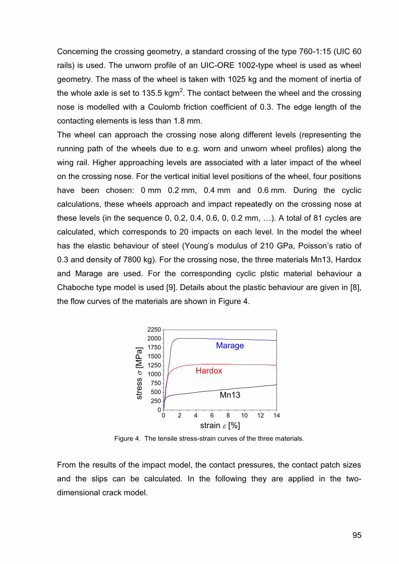
95
Concerning the crossing geometry, a standard crossing of the type 760-1:15 (UIC 60
rails) is used. The unworn profile of an UIC-ORE 1002-type wheel is used as wheel
geometry. The mass of the wheel is taken with 1025 kg and the moment of inertia of
the whole axle is set to 135.5 kgm2. The contact between the wheel and the crossing
nose is modelled with a Coulomb friction coefficient of 0.3. The edge length of the
contacting elements is less than 1.8 mm.
The wheel can approach the crossing nose along different levels (representing the
running path of the wheels due to e.g. worn and unworn wheel profiles) along the
wing rail. Higher approaching levels are associated with a later impact of the wheel
on the crossing nose. For the vertical initial level positions of the wheel, four positions
have been chosen: 0 mm 0.2 mm, 0.4 mm and 0.6 mm. During the cyclic
calculations, these wheels approach and impact repeatedly on the crossing nose at
these levels (in the sequence 0, 0.2, 0.4, 0.6, 0, 0.2 mm, …). A total of 81 cycles are
calculated, which corresponds to 20 impacts on each level. In the model the wheel
has the elastic behaviour of steel (Young’s modulus of 210 GPa, Poisson’s ratio of
0.3 and density of 7800 kg). For the crossing nose, the three materials Mn13, Hardox
and Marage are used. For the corresponding cyclic plstic material behaviour a
Chaboche type model is used [9]. Details about the plastic behaviour are given in [8],
the flow curves of the materials are shown in Figure 4.
0 2 4 6 8 10 12 140
250
500
750
1000
1250
1500
1750
2000
2250
Mn13
Hardox
str
ess
[M
Pa
]
strain [%]
Marage
Figure 4. The tensile stress-strain curves of the three materials.
From the results of the impact model, the contact pressures, the contact patch sizes
and the slips can be calculated. In the following they are applied in the two-
dimensional crack model.
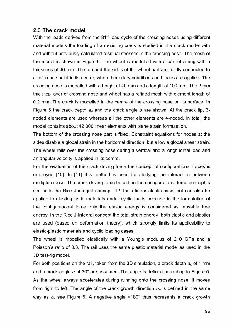
96
2.3 The crack model
With the loads derived from the 81st load cycle of the crossing noses using different
material models the loading of an existing crack is studied in the crack model with
and without previously calculated residual stresses in the crossing nose. The mesh of
the model is shown in Figure 5. The wheel is modelled with a part of a ring with a
thickness of 40 mm. The top and the sides of the wheel part are rigidly connected to
a reference point in its centre, where boundary conditions and loads are applied. The
crossing nose is modelled with a height of 40 mm and a length of 100 mm. The 2 mm
thick top layer of crossing nose and wheel has a refined mesh with element length of
0.2 mm. The crack is modelled in the centre of the crossing nose on its surface. In
Figure 5 the crack depth ad and the crack angle α are shown. At the crack tip, 3-
noded elements are used whereas all the other elements are 4-noded. In total, the
model contains about 42 000 linear elements with plane strain formulation.
The bottom of the crossing nose part is fixed. Constraint equations for nodes at the
sides disable a global strain in the horizontal direction, but allow a global shear strain.
The wheel rolls over the crossing nose during a vertical and a longitudinal load and
an angular velocity is applied in its centre.
For the evaluation of the crack driving force the concept of configurational forces is
employed [10]. In [11] this method is used for studying the interaction between
multiple cracks. The crack driving force based on the configurational force concept is
similar to the Rice J-integral concept [12] for a linear elastic case, but can also be
applied to elastic-plastic materials under cyclic loads because in the formulation of
the configurational force only the elastic energy is considered as reusable free
energy. In the Rice J-Integral concept the total strain energy (both elastic and plastic)
are used (based on deformation theory), which strongly limits its applicability to
elastic-plastic materials and cyclic loading cases.
The wheel is modelled elastically with a Young’s modulus of 210 GPa and a
Poisson’s ratio of 0.3. The rail uses the same plastic material model as used in the
3D test-rig model.
For both positions on the rail, taken from the 3D simulation, a crack depth ad of 1 mm
and a crack angle of 30° are assumed. The angle is defined according to Figure 5.
As the wheel always accelerates during running onto the crossing nose, it moves
from right to left. The angle of the crack growth direction e is defined in the same
way as , see Figure 5. A negative angle <180° thus represents a crack growth
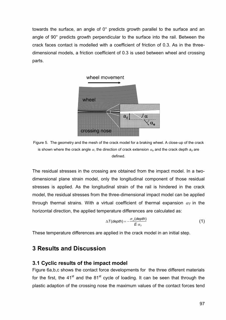
97
towards the surface, an angle of 0° predicts growth parallel to the surface and an
angle of 90° predicts growth perpendicular to the surface into the rail. Between the
crack faces contact is modelled with a coefficient of friction of 0.3. As in the three-
dimensional models, a friction coefficient of 0.3 is used between wheel and crossing
parts.
Figure 5. The geometry and the mesh of the crack model for a braking wheel. A close-up of the crack
is shown where the crack angle , the direction of crack extension e and the crack depth ad are
defined.
The residual stresses in the crossing are obtained from the impact model. In a two-
dimensional plane strain model, only the longitudinal component of those residual
stresses is applied. As the longitudinal strain of the rail is hindered in the crack
model, the residual stresses from the three-dimensional impact model can be applied
through thermal strains. With a virtual coefficient of thermal expansion T in the
horizontal direction, the applied temperature differences are calculated as:
( )( ) x
T
depthT depth
E
(1)
These temperature differences are applied in the crack model in an initial step.
3 Results and Discussion
3.1 Cyclic results of the impact model
Figure 6a,b,c shows the contact force developments for the three different materials
for the first, the 41st and the 81st cycle of loading. It can be seen that through the
plastic adaption of the crossing nose the maximum values of the contact forces tend

98
to increase. This small increase of the vertical contact forces is not so important as
the contact stresses are strongly reduced by the plastic deformation, see section 3.2.
In the two harder materials Marage and Hardox this effect is only small. For Mn13,
the plastic behaviour of the crossing nose leads to a contact force development in
which the second maximum becomes bigger than the first one. The cause for these
changes with proceeding cycles is the longitudinal development of the crossing’s
profile, which was approximately flat in the nominal geometry prior to deformation. In
Figure 6d this profile is plotted after 80 cycles of loading for the three materials. The
results for Marage approximately correspond with the nominal profile. For Hardox,
there is a small dent in the region of the wheel’s impact (wheel position of 0.1 m) with
a depth of about 40 m. The material Mn13 has a bigger dent with a depth of about
400 m. This explains the increase of the second peak in the contact force
development. The first impact of the wheel with the crossing nose is damped and a
bigger impact occurs at the end of the dent. In Table 1 the highest values of the
vertical contact forces and accumulated equivalent plastic strains (PEEQ) are shown.
The change in the longitudinal profiles is associated with a maximum PEEQ of 30%
in the Mn13, 6.8% in the Hardox and 0.76% in the Marage crossing. Note that the
initial position of impact can cause an increase of the second contact force peak of
the Mn13 crossing. In the following investigation of the loading of surface cracks in
the crossing only the first peak of the contact forces is chosen to transfer the loads to
the crack model. More details about the impact model are given in [8]
Table 1. Results of the impact model
Material Mn13 Hardox Marage
Max PEEQ
(80 cycles)
30 % 6.8 % 0.76 %
Highest contact force (81st
cycle)
225 kN 198 kN 193 kN
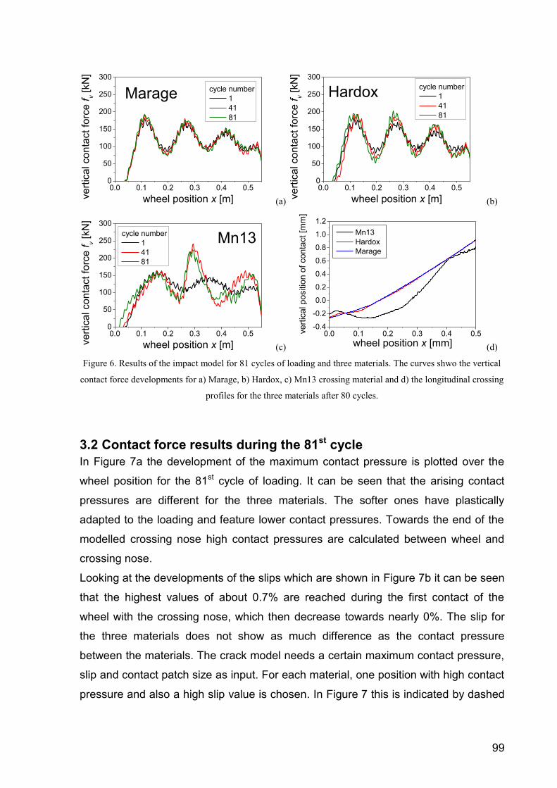
99
0.0 0.1 0.2 0.3 0.4 0.50
50
100
150
200
250
300
Marage
ve
rtic
al co
nta
ct
forc
e f
v [
kN
]
wheel position x [m]
cycle number
1
41
81
(a)
0.0 0.1 0.2 0.3 0.4 0.50
50
100
150
200
250
300
Hardox
ve
rtic
al co
nta
ct
forc
e f
v [
kN
]
wheel position x [m]
cycle number
1
41
81
(b)
0.0 0.1 0.2 0.3 0.4 0.50
50
100
150
200
250
300
ve
rtic
al co
nta
ct
forc
e f
v [
kN
]
wheel position x [m]
cycle number
1
41
81
Mn13
(c)
0.0 0.1 0.2 0.3 0.4 0.5-0.4
-0.2
0.0
0.2
0.4
0.6
0.8
1.0
1.2
Mn13
Hardox
Marage
vert
ical positio
n o
f conta
ct
[mm
]
wheel position x [mm] (d)
Figure 6. Results of the impact model for 81 cycles of loading and three materials. The curves shwo the vertical
contact force developments for a) Marage, b) Hardox, c) Mn13 crossing material and d) the longitudinal crossing
profiles for the three materials after 80 cycles.
3.2 Contact force results during the 81st cycle
In Figure 7a the development of the maximum contact pressure is plotted over the
wheel position for the 81st cycle of loading. It can be seen that the arising contact
pressures are different for the three materials. The softer ones have plastically
adapted to the loading and feature lower contact pressures. Towards the end of the
modelled crossing nose high contact pressures are calculated between wheel and
crossing nose.
Looking at the developments of the slips which are shown in Figure 7b it can be seen
that the highest values of about 0.7% are reached during the first contact of the
wheel with the crossing nose, which then decrease towards nearly 0%. The slip for
the three materials does not show as much difference as the contact pressure
between the materials. The crack model needs a certain maximum contact pressure,
slip and contact patch size as input. For each material, one position with high contact
pressure and also a high slip value is chosen. In Figure 7 this is indicated by dashed
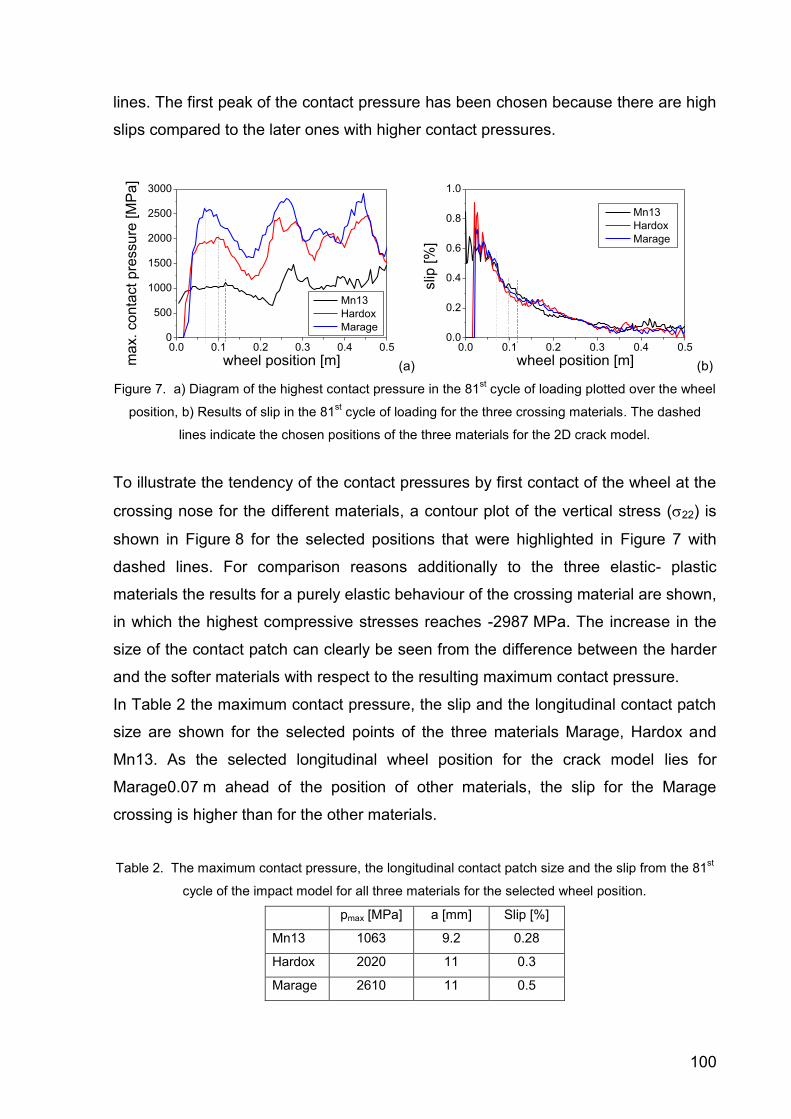
100
lines. The first peak of the contact pressure has been chosen because there are high
slips compared to the later ones with higher contact pressures.
0.0 0.1 0.2 0.3 0.4 0.50
500
1000
1500
2000
2500
3000
Mn13
Hardox
Marage
ma
x.
co
nta
ct
pre
ssu
re [
MP
a]
wheel position [m] (a)
0.0 0.1 0.2 0.3 0.4 0.50.0
0.2
0.4
0.6
0.8
1.0
Mn13
Hardox
Marage
slip
[%
]
wheel position [m] (b)
Figure 7. a) Diagram of the highest contact pressure in the 81st cycle of loading plotted over the wheel
position, b) Results of slip in the 81st cycle of loading for the three crossing materials. The dashed
lines indicate the chosen positions of the three materials for the 2D crack model.
To illustrate the tendency of the contact pressures by first contact of the wheel at the
crossing nose for the different materials, a contour plot of the vertical stress (22) is
shown in Figure 8 for the selected positions that were highlighted in Figure 7 with
dashed lines. For comparison reasons additionally to the three elastic- plastic
materials the results for a purely elastic behaviour of the crossing material are shown,
in which the highest compressive stresses reaches -2987 MPa. The increase in the
size of the contact patch can clearly be seen from the difference between the harder
and the softer materials with respect to the resulting maximum contact pressure.
In Table 2 the maximum contact pressure, the slip and the longitudinal contact patch
size are shown for the selected points of the three materials Marage, Hardox and
Mn13. As the selected longitudinal wheel position for the crack model lies for
Marage0.07 m ahead of the position of other materials, the slip for the Marage
crossing is higher than for the other materials.
Table 2. The maximum contact pressure, the longitudinal contact patch size and the slip from the 81st
cycle of the impact model for all three materials for the selected wheel position.
pmax [MPa] a [mm] Slip [%]
Mn13 1063 9.2 0.28
Hardox 2020 11 0.3
Marage 2610 11 0.5
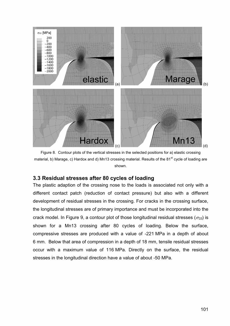
101
(a) (b)
(c) (d)
Figure 8. Contour plots of the vertical stresses in the selected positions for a) elastic crossing
material, b) Marage, c) Hardox and d) Mn13 crossing material. Results of the 81st cycle of loading are
shown.
3.3 Residual stresses after 80 cycles of loading
The plastic adaption of the crossing nose to the loads is associated not only with a
different contact patch (reduction of contact pressure) but also with a different
development of residual stresses in the crossing. For cracks in the crossing surface,
the longitudinal stresses are of primary importance and must be incorporated into the
crack model. In Figure 9, a contour plot of those longitudinal residual stresses (33) is
shown for a Mn13 crossing after 80 cycles of loading. Below the surface,
compressive stresses are produced with a value of -221 MPa in a depth of about
6 mm. Below that area of compression in a depth of 18 mm, tensile residual stresses
occur with a maximum value of 116 MPa. Directly on the surface, the residual
stresses in the longitudinal direction have a value of about -50 MPa.

102
Figure 9. Contour plot of the residual stresses in the longitudinal direction after the 80th load cycle in
the Mn13 crossing (results of the 80th cycle are the input for the 81
st cycle). Cross- section at the
position of the highest contact pressure after cycle 81.
In Figure 10, the longitudinal residual stresses are plotted in depth direction of the
crossing for the three materials. As longitudinal position at the crossing nose a cross-
section is chosen where the highest contact pressures appear. Table 3 shows the
highest arising residual stresses for the three materials and the distance from the
surface of their maxima as well as the longitudinal residual stresses in the assumed
depth of the crack tip.
200 0 -200 -400 -60020
18
16
14
12
10
8
6
4
2
0
crack depth
Dis
tan
ce
fro
m S
urf
ace
[m
m]
longitudinal stress l [MPa]
Crossing material
Mn13
Hardox
Marage
Figure 10. Contour plot of the residual stresses in the longitudinal direction after the 80th load cycle in
the Mn13 crossing. Cross- section at the position of the highest contact pressure in cycle 81.
It can be seen that for Hardox and Marage, even higher residual stresses develop
than in the initially soft Mn13 material For Hardox, the highest compressive stresses
reach a value of -495 MPa in a depth of 2.4 mm. For Marage, the highest
compressive residual stresses are directly on the surface with a value of -366 MPa.
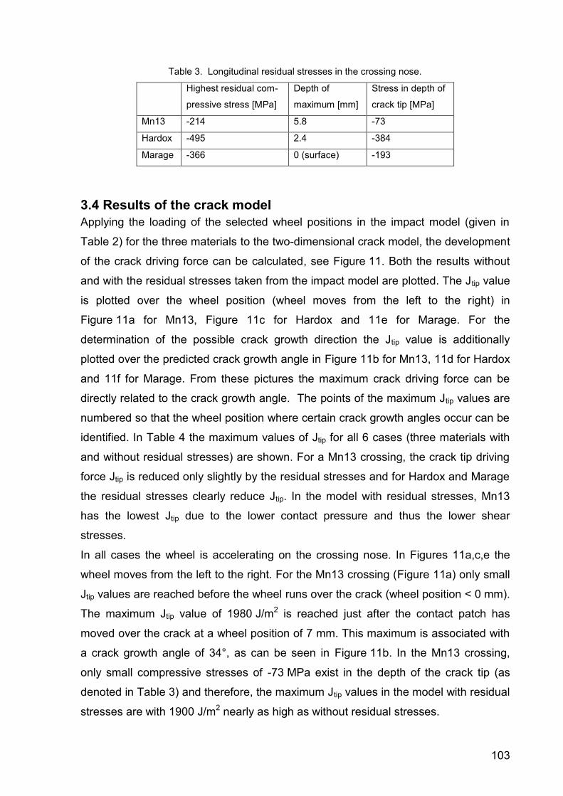
103
Table 3. Longitudinal residual stresses in the crossing nose.
Highest residual com-
pressive stress [MPa]
Depth of
maximum [mm]
Stress in depth of
crack tip [MPa]
Mn13 -214 5.8 -73
Hardox -495 2.4 -384
Marage -366 0 (surface) -193
3.4 Results of the crack model
Applying the loading of the selected wheel positions in the impact model (given in
Table 2) for the three materials to the two-dimensional crack model, the development
of the crack driving force can be calculated, see Figure 11. Both the results without
and with the residual stresses taken from the impact model are plotted. The Jtip value
is plotted over the wheel position (wheel moves from the left to the right) in
Figure 11a for Mn13, Figure 11c for Hardox and 11e for Marage. For the
determination of the possible crack growth direction the Jtip value is additionally
plotted over the predicted crack growth angle in Figure 11b for Mn13, 11d for Hardox
and 11f for Marage. From these pictures the maximum crack driving force can be
directly related to the crack growth angle. The points of the maximum Jtip values are
numbered so that the wheel position where certain crack growth angles occur can be
identified. In Table 4 the maximum values of Jtip for all 6 cases (three materials with
and without residual stresses) are shown. For a Mn13 crossing, the crack tip driving
force Jtip is reduced only slightly by the residual stresses and for Hardox and Marage
the residual stresses clearly reduce Jtip. In the model with residual stresses, Mn13
has the lowest Jtip due to the lower contact pressure and thus the lower shear
stresses.
In all cases the wheel is accelerating on the crossing nose. In Figures 11a,c,e the
wheel moves from the left to the right. For the Mn13 crossing (Figure 11a) only small
Jtip values are reached before the wheel runs over the crack (wheel position < 0 mm).
The maximum Jtip value of 1980 J/m2 is reached just after the contact patch has
moved over the crack at a wheel position of 7 mm. This maximum is associated with
a crack growth angle of 34°, as can be seen in Figure 11b. In the Mn13 crossing,
only small compressive stresses of -73 MPa exist in the depth of the crack tip (as
denoted in Table 3) and therefore, the maximum Jtip values in the model with residual
stresses are with 1900 J/m2 nearly as high as without residual stresses.
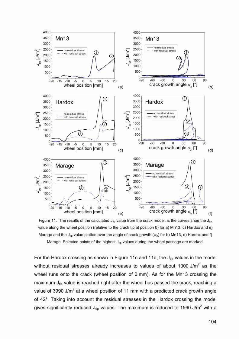
104
-20 -15 -10 -5 0 5 10 15 200
500
1000
1500
2000
2500
3000
3500
4000
no residual stress
with residual stress
Jtip [J/m
2]
wheel position [mm]
Mn13
12
(a)
-90 -60 -30 0 30 60 900
500
1000
1500
2000
2500
3000
3500
4000
no residual stress
with residual stress
Jtip [
J/m
2]
crack growth angle e [°]
Mn13
1
2
(b)
-20 -15 -10 -5 0 5 10 15 200
500
1000
1500
2000
2500
3000
3500
4000
no residual stress
with residual stress
Jtip [
J/m
2]
wheel position [mm]
Hardox1
2
3
(c)
-90 -60 -30 0 30 60 900
500
1000
1500
2000
2500
3000
3500
4000
no residual stress
with residual stress
Jtip [
J/m
2]
crack growth angle e [°]
Hardox1
2
3
(d)
-20 -15 -10 -5 0 5 10 15 200
500
1000
1500
2000
2500
3000
3500
4000
no residual stress
with residual stress
Jtip [
J/m
2]
wheel position [mm]
Marage1
23
(e)
-90 -60 -30 0 30 60 900
500
1000
1500
2000
2500
3000
3500
4000
no residual stress
with residual stress
Jtip [J/m
2]
crack growth angle e [°]
Marage1
23
(f)
Figure 11. The results of the calculated Jtip value from the crack model. is the curves shoe the Jtip
value along the wheel position (relative to the crack tip at position 0) for a) Mn13, c) Hardox and e)
Marage and the Jtip value plotted over the angle of crack growth (e) for b) Mn13, d) Hardox and f)
Marage. Selected points of the highest Jtip values during the wheel passage are marked.
For the Hardox crossing as shown in Figure 11c and 11d, the Jtip values in the model
without residual stresses already increases to values of about 1000 J/m2 as the
wheel runs onto the crack (wheel position of 0 mm). As for the Mn13 crossing the
maximum Jtip value is reached right after the wheel has passed the crack, reaching a
value of 3990 J/m2 at a wheel position of 11 mm with a predicted crack growth angle
of 42°. Taking into account the residual stresses in the Hardox crossing the model
gives significantly reduced Jtip values. The maximum is reduced to 1560 J/m2 with a

105
steeper crack angle of 51°. When the wheel is nearly directly over the crack (wheel
position of -3 mm), there is another maximum of the Jtip value calculated in presence
of residual stresses. This maximum, however, reaches Jtip values of not more than
450 J/m2.
Table 4. Maximum values of the Jtip value and the corresponding crack growth angles for the three
materials and the two cases without and with residual stresses.
J integral
Jtip [J/m2]
Crack growth
angle e [°]
Mn13 1980 34
Mn13, residual stress 1900 35
Hardox 3990 42
Hardox, residual stress 1560 51
Marage 3720 45
Marage, residual stress 1370 49
The results for the Marage crossing are shown in Figure 11e and Figure 11f. The
development of the Jtip value for the model without residual stresses is similar to the
results of Hardox, but with lower Jtip values with a maximum of 3720 J/m2 at a wheel
position of 12 mm. The crack growth angle for that maximum is 45°. By introducing
residual stresses from the impact model the Jtip value is also considerably reduced.
The maximum reaches a value of 1370 J/m2 at a wheel position of 12 mm, which is
even lower than the calculated value of the Mn13 crossing. In the cases with applied
residual stresses the Jtip value has another peak at a position nearly directly over the
crack (wheel position of -2 mm). Here it reaches a value of 1400 J/m2 with a crack
angle of 75°. For the critical Jtip values a series of experiments is necessary. This will
be the subject of a future research project.
4 Conclusions
Models on three length scales are employed to calculate the driving force on existing
cracks in crossing noses. Three materials with different hardnesses are compared:
the very soft Manganese steel Mn13, the Hardox steel with a higher hardness and
the very hard maraging steel Marage. On the level of the impact model the plastic
adaption of the crossing nose to the loading is described, which reduces the contact
pressures and shear stresses and thus the driving forces on the crack. It is shown
106
that the soft Mn13 steel features less than half the contact pressures as the hard
Marage steel. This is probably one reason for the good performance of Manganese
steel used in crossings. The impact model also calculates the residual stresses in the
crossing. The longitudinal residual stresses can be applied in the crack model. It is
shown that the maximum of those compressive stresses moves towards the surface
with increasing hardness of the crossing. Applying the loads from the impact model in
the crack model finally shows the effect of the plastic adaption and the residual
stresses on Jtip. In the calculations without residual stresses the severely adapting
Manganese steel shows a lower crack tip loading than the harder Hardox and
Marage steels. It is shown, however, that the residual stresses have nearly no effect
on the crack driving force in Mn13 for the assumed crack depth. For Hardox and
Marage crossings the residual stresses significantly reduce the driving force on the
crack to values even less than in the Mn13 crossing. Without data from crack growth
experiments (for cracks loaded in the shear mode, the so-called Mode II) no final
statement can be made about the performance of the different materials used as
crossings. The different fracture toughnesses need to be carefully taken into account
and may shift the predicted tendency to develop cracks. The paper is intended to
show a straight-forward procedure to evaluate possible rolling contact fatigue in this
extremely complex case of a wheel running over a crossing nose. The approach
shows that the whole system with the dynamic response, the cyclic plastic material
behaviour (geometric adaption of the crossing and development of residual stresses)
and the crack loading has to be regarded for describing and understanding the
damage development.
Acknowledgements
Financial support by the Austrian Federal Government (in particular from the
Bundesministerium für Verkehr, Innovation und Technologie and the Bundes-
ministerium für Wirtschaft und Arbeit) and the Styrian Provincial Government,
represented by Österreichische Forschungsförderungsgesellschaft mbH and by
Steirische Wirtschaftsförderungsgesellschaft mbH, within the research activities of
the K2 Competence Centre on “Integrated Research in Materials, Processing and
Product Engineering”, operated by the Materials Center Leoben Forschung GmbH in
the framework of the Austrian COMET Competence Centre Programme, is gratefully
acknowledged.
107
References
[1] E. Kassa, Dynamic train-turnout interaction: mathematical modelling,
numerical simulation and field testing, PhD Thesis, Chalmers University of
Technology, Gothenburg, Sweden, 2007.
[2] M. Pletz, W. Daves, H. Ossberger, A Wheel Set / Crossing Model Regarding
Impact, Sliding and Deformation- Explicit Finite Element Approach, Wear
(submitted), (2012).
[3] M. Pletz, W. Daves, H. Ossberger, A Wheel Passing a Frog Nose- Dynamic
Finite Element Investigation of High Axle Loads, Proceedings of the Institution
of Mechanical Engineers, Part F: Journal of Rail and Rapid Transit, (2012).
[4] F.C. Liu, B. Lv, F.C. Zhang, S. Yang, Enhanced work hardening in Hadfield
steel during explosive treatment, Materials Letters, 65 2333-2336.
[5] Abaqus, Abaqus user's manual, version 6.9, in.
[6] M. Pletz, W. Daves, H. Ossberger, A Dynamical Wheel Set: Crossing Model
Regarding Impact, Sliding and Deformation, in: 8th International Conference
on Contact Mechanics and Wear of Rail/Wheel Systems, Florence, Italy, 2009,
pp. 801-809.
[7] M. Pletz, W. Daves, H. Ossberger, Dynamic Finite Element Model of a Wheel
Passing a Crossing Nose, in: Tenth international conference on
computational structures technology, Valencia, Spain, on-line, 2010.
[8] M. Pletz, W. Daves, S. Eck, H. Ossberger, The Plastic Adaption of Railway
Crossings due to Dynamic Contact Loading - Explicit Finite Element Study,
Tribology Inetrnational (submitted), (2012).
[9] J.L. Chaboche, Constitutive equations for cyclic plasticity and cyclic
viscoplasticity, International Journal of Plasticity, 5 (1989) 247-302.
[10] N.K. Simha, F.D. Fischer, G.X. Shan, C.R. Chen, O. Kolednik, J-integral and
crack driving force in elastic–plastic materials, Journal of the Mechanics and
Physics of Solids, 56 (2008) 2876-2895.
[11] J. Tillberg, F. Larsson, K. Runesson, A study of multiple crack interaction at
rolling contact fatigue loading of rails, Proceedings of the Institution of
Mechanical Engineers, Part F: Journal of Rail and Rapid Transit, 223 (2009)
319-330.
[12] J.R. Rice, A.S.o.M. Engineers, A path independent integral and the
approximate analysis of strain concentration by notches and cracks, ASME,

108
1968.