1

Damage detection of base-isolated buildings using multi-inputs multi-

outputs subspace identification

Reiki Yoshimoto1, Akira Mita2, Keiichi Okada3

1Researcher, Safety Science and Policy Department, Mitsubishi Research Institute, Tokyo, JAPAN

2Professor, Department of System Design Engineering, Keio University, Yokohama, JAPAN

3Senior Researcher, Institute of Technology, Shimizu Corporation, Tokyo, JAPAN

Correspondence to:

Prof. Akira Mita Department of System Design Engineering, Keio University 3-14-1 Hiyoshi, Kohoku-ku, Yokohama 223-8522, Japan Tel & Fax: +81 45-566-1776 Email: mita@sd.keio.ac.jp

2

SUMMARY

A damage detection algorithm of structural health monitoring systems for base-isolated

buildings is proposed. The algorithm consists of the multiple-inputs multiple-outputs

subspace identification method and the complex modal analysis. The algorithm is

applicable to linear and nonlinear systems. The story stiffness and damping as damage

indices of a shear structure are identified by the algorithm. The algorithm is further

tuned for base-isolated buildings considering their unique dynamic characteristics by

simplifying the systems to single-degree of freedom systems. The isolation layer and the

superstructure of a base-isolated building are treated as separate substructures as they

are distinctly different in their dynamic properties. The effectiveness of the algorithm is

evaluated through the numerical analysis and experiment. Finally, the algorithm is

applied to the existing 7-story base-isolated building that is equipped with an internet-

based monitoring system.

Keywords: system identification; subspace identification; MIMO; health monitoring;

base-isolation

3

1. INTRODUCTION

There is a growing interest in assessing structural integrity of buildings and

infrastructures associated with their deterioration and natural hazards. To ensure the

integrity and the safety of a building, an SHM (Structural Health Monitoring) system is

one of solutions for prompt and quantitative evaluation.

For the purpose of damage detection, damage indices that are strongly correlated to

the structural damages must be identified precisely. Many studies are still being

conducted in this area [1]. The conventional damage indices such as modal frequencies

[2], mode shapes [3], curvature mode shapes [4] and modal flexibilities [5] are

considered not accurate enough for local and quantitative damage detection. When a

damage occurs in some layers of the building due to, say, a large earthquake, the

stiffness will be reduced. In this case, the story stiffness may be a good index. There are

some studies, such as the method for online estimation of the stiffness matrix using

extended Kalman filter [6], estimation of the story stiffness and viscous damping using

transfer functions [7], parallel estimation of the story parameters [8] and so on. The

accuracy of these methods highly depends on the noise level contained in the data. In

this study, a new and stable algorithm to obtain story stiffness and damping using the

subspace identification method is proposed.

The MIMO models are known to be suitable for representing behaviors in three-

dimensional space. However, in civil engineering field single-input and single-output

(SISO) models have been conventionally used. This is mainly due to the lack of tools to

take care of multi-inputs and multi-output (MIMO) models and the difficulty to identify

4

the proper correlation between inputs and outputs for the specific mode. The proposed

algorithm resolves these difficulties by using the subspace identification for MIMO

models and by introducing participation factors.

The isolation devices are designed to absorb major components of energy input for a

base-isolated building when subject to a large earthquake. However, there exists a

certain probability to exceed the design capacity for the extreme earthquake. The

structural integrity of the isolated building is no longer guaranteed in such a case. In the

fear of the possibility of suffering from damages to the isolated building, incorporating

an SHM system may have a good rationale for immediate diagnosis of the structural

integrity as well as continuous observation of material deterioration. A conventional

building absorbs the seismic energy mainly at beam-column joints of the supporting

frames that have a high-degree of complexity; this implies that scenarios for structural

damages vary depending on the characteristics of earthquakes. In addition, accurate

simulation for each scenario is very difficult. The damage scenario for a base-isolated

structure is much simpler and more accurate than the situation for a conventional

building. Our strategy is to get the most out of this simplicity in the purpose of

establishing the SHM system for base-isolated buildings.

5

2. FORMULATION

2.1. Model description

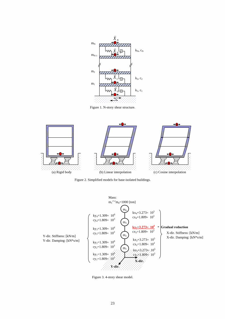
An N-story shear structure consisting of N masses, N springs and N dampers is

considered as shown in Figure 1. Mass distribution is assumed given. The acceleration

measured at the ith floor is described by iX&& . The story stiffness indicated by the spring

ik and the story damping indicated by the damper ic are unknown.

2.2. MOESP method

The MOESP method that is one of the subspace model identification methods is used as

a basis of our algorithm for identifying story stiffness and damping. The subspace

model identification is a method to obtain a state space model from input and output

data using Hankel matrices. In this study, the subspace model identification method was

employed because the method is easily applicable to MIMO models to improve the

accuracy of the identification. As we are interested in state-space representation, we

chose subspace model identification method among others. As an additional benefit,

stability of identification can be evaluated by singular value decomposition in the

course of this identification.

The linear state equations in a discrete form are given by:

kkk BuAxx +=+1 (1)

where nℜ∈x stands for the n-dimensional state vector. The vector mℜ∈u is the

m-dimensional input vector. The corresponding output equations are:

6

kkk DuCxy += (2)

where the vector lℜ∈y is the l-dimensional output vector. Among many subspace

identification methods, the MOESP algorithm [9] is utilized to realize system matrices

A, B, C, D from measured inputs u and outputs y using QR-factorization and singular

value decomposition (SVD). The MOESP algorithm is numerically stable and is suited

for real time identification. Introducing Hankel matrices, the output equations become:

[ ]

⎥⎥⎥⎥⎥

⎦

⎤

⎢⎢⎢⎢⎢

⎣

⎡

⎥⎥⎥⎥⎥⎥

⎦

⎤

⎢⎢⎢⎢⎢⎢

⎣

⎡

+

⎥⎥⎥⎥

⎦

⎤

⎢⎢⎢⎢

⎣

⎡

=

⎥⎥⎥⎥⎥

⎦

⎤

⎢⎢⎢⎢⎢

⎣

⎡

−++

+

−−

−−++

+

11

132

21

32

21

111

132

21

jiii

j

j

ii

j

ijiii

j

j

uuu

uuuuuu

DCBBCABCA

CBCAB0DCB

D

xxx

CA

CAC

yyy

yyyyyy

L

OM

L

L

OM

O

LM

L

OM

L

(3)

Equation (3) can be rewritten in a more compact form as:

ijijiij UTXOY += (4)

where, Oi and Ti are called the extended observability matrix and the Toeplitz matrix,

respectively. jmiij

×⋅ℜ∈U and jliij

×⋅ℜ∈Y are called block Hankel matrices (with i

block rows, j columns). The whole Hankel matrix H containing the measured input-

output data is then constructed. Applying the QR-factorization, the LQ decomposition

of the matrix is given by:

⎥⎥⎦

⎤

⎢⎢⎣

⎡

+=

==⎥

⎦

⎤⎢⎣

⎡⎥⎦

⎤⎢⎣

⎡=⎥

⎦

⎤⎢⎣

⎡=

TTij

Tij

T

T

ij

ij

222121

111

2

1

2221

11

QLQLY

QLU

QQ

LL0L

YU

H (5)

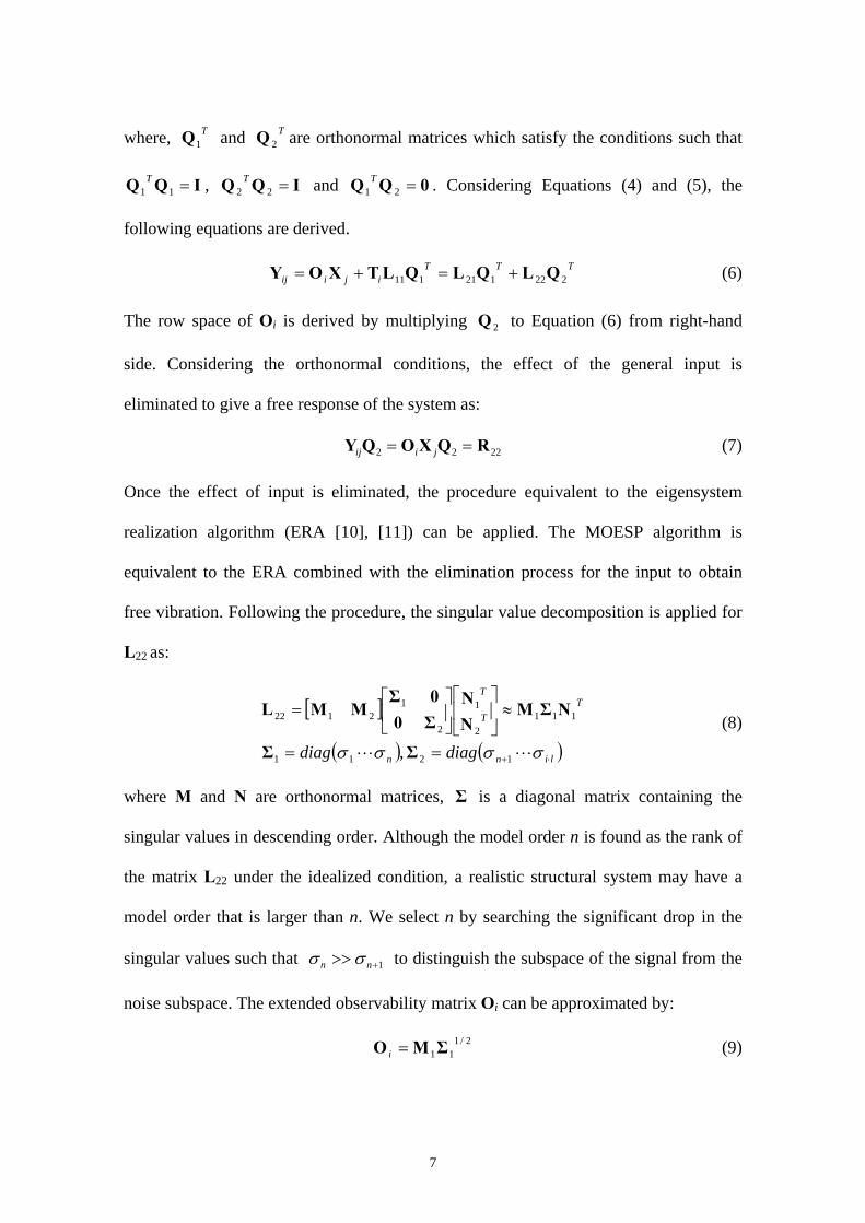
7

where, T1Q and T

2Q are orthonormal matrices which satisfy the conditions such that

IQQ =11T , IQQ =22

T and 0QQ =21T . Considering Equations (4) and (5), the

following equations are derived.

TTTijiij 222121111 QLQLQLTXOY +=+= (6)

The row space of Oi is derived by multiplying 2Q to Equation (6) from right-hand

side. Considering the orthonormal conditions, the effect of the general input is

eliminated to give a free response of the system as:

2222 RQXOQY == jiij (7)

Once the effect of input is eliminated, the procedure equivalent to the eigensystem

realization algorithm (ERA [10], [11]) can be applied. The MOESP algorithm is

equivalent to the ERA combined with the elimination process for the input to obtain

free vibration. Following the procedure, the singular value decomposition is applied for

L22 as:

[ ]

( ) ( )linn

TT

T

diagdiag ⋅+==

≈⎥⎦

⎤⎢⎣

⎡⎥⎦

⎤⎢⎣

⎡=

σσσσ LL 1211

1112

1

2

12122

,ΣΣ

NΣMNN

Σ00Σ

MML (8)

where M and N are orthonormal matrices, Σ is a diagonal matrix containing the

singular values in descending order. Although the model order n is found as the rank of

the matrix L22 under the idealized condition, a realistic structural system may have a

model order that is larger than n. We select n by searching the significant drop in the

singular values such that 1+>> nn σσ to distinguish the subspace of the signal from the

noise subspace. The extended observability matrix Oi can be approximated by:

2/111ΣMO =i (9)

8

Once the extended observability matrix Oi is obtained, the matrix C is realized by

extracting the top block. The matrix A is computed based on the shift invariance of Oi

as:

↑−

+−

↑−−

⋅=

=⋅

11

11

ii

ii

OOA

OAO (10)

where, 1−iO is the matrix obtained by deleting the last block row of Oi, ↑−1iO is the

upper-shifted matrix by one block row, and ( )+• represents the pseudo-inverse of a

matrix. In this study, we don’t have to estimate the system matrices B and D because

they contain no modal information.

From eigenvalue analysis of the matrix A, we obtain the ith pole iz p and

eigenvector izφ in z-domain. Considering the relationship between z- and s-domain,

iz p is converted into iλ , which is the pole in continuous-time system, i.e. in s-

domain. In addition, by pre-multiplying the matrix C to izφ , we can obtain a complex

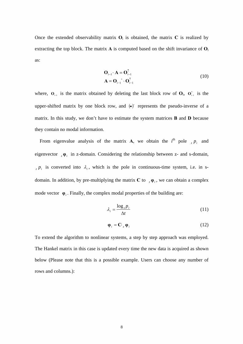
mode vector iφ . Finally, the complex modal properties of the building are:

tpiz

i ∆=

logλ (11)

izi φCφ ⋅= (12)

To extend the algorithm to nonlinear systems, a step by step approach was employed.

The Hankel matrix in this case is updated every time the new data is acquired as shown

below (Please note that this is a possible example. Users can choose any number of

rows and columns.):

9

⎥⎥⎥⎥

⎦

⎤

⎢⎢⎢⎢

⎣

⎡

=

76543

65432

54321

43210

0

yyyyyyyyyyyyyyyyyyyy

Y ⇒

⎥⎥⎥⎥

⎦

⎤

⎢⎢⎢⎢

⎣

⎡

=

87654

76543

65432

54321

1

yyyyyyyyyyyyyyyyyyyy

Y

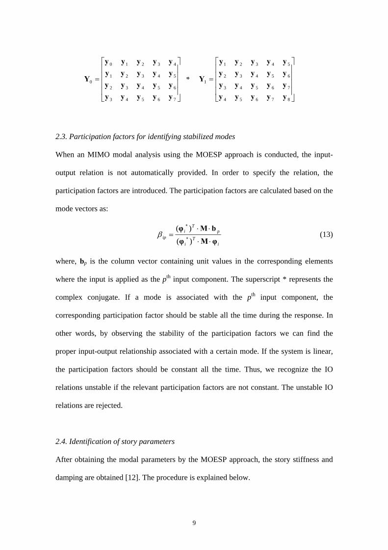
2.3. Participation factors for identifying stabilized modes

When an MIMO modal analysis using the MOESP approach is conducted, the input-

output relation is not automatically provided. In order to specify the relation, the

participation factors are introduced. The participation factors are calculated based on the

mode vectors as:

i

Ti

pT

iip φMφ

bMφ

⋅⋅

⋅⋅= ∗

∗

)(

)(β (13)

where, bp is the column vector containing unit values in the corresponding elements

where the input is applied as the pth input component. The superscript * represents the

complex conjugate. If a mode is associated with the pth input component, the

corresponding participation factor should be stable all the time during the response. In

other words, by observing the stability of the participation factors we can find the

proper input-output relationship associated with a certain mode. If the system is linear,

the participation factors should be constant all the time. Thus, we recognize the IO

relations unstable if the relevant participation factors are not constant. The unstable IO

relations are rejected.

2.4. Identification of story parameters

After obtaining the modal parameters by the MOESP approach, the story stiffness and

damping are obtained [12]. The procedure is explained below.

10

An inertia force at the jth mass fj is calculated as:

∑=

⋅−=N

jkkkj Xmf && (14)

where, kx&& is the acceleration at the kth mass. The inertia force should be equal to the

spring and damping forces as:

)()( 11 −− −+−= jjjjjjj XXcXXkf && (15)

where, kj and cj are the story stiffness and damping, respectively. These parameters can

be directly identified using acceleration time histories [8]. However, the identification

procedure involves integrators in the course of deriving the relative displacement and

velocity. The precision of the estimation, therefore, highly depends on the noise level

and initial values taken for estimation. Instead of using acceleration time histories, we

propose the use of modal parameters to estimate story stiffness and damping. The

harmonic displacement response at the jth mass that vibrates in the i-th mode can be

expressed in the form:

tjiji

ietX λφ ⋅= )()( )( (16)

Therefore, the relative displacement and velocity are obtained by:

{ }{ } t

ijijijijiji

tjijijijiji

i

i

etXtXtd

etXtXtdλ

λ

λφφ

φφ

⋅−=−=

⋅−=−=

−−

−−

)1()()1()()(

)1()()1()()(

)()()(

)()()(&&&

(17)

The inertia force fi(j) associated with the ith mode at the jth story is given by:

( ) ( ) ∑∑ ==⋅−=⋅−=

N

jk kikt

iN

jk kikji metXmtf i)(

2)()( φλ λ&& (18)

Restricting ki(j) and ci(j) to be real numbers, the equation of equilibrium with respect the

force acting on the jth story is derived as:

( ) ( ) ( )ttctk jijijijiji )()()()()( fdd =⋅+⋅ & (19)

11

Solving the above equation in least square manner, the stiffness and damping of the jth

story should be obtained. It is noted that we do not use the ith modal mass. A free

vibration with the shape of the ith mode is assumed to obtain the inertia force fi(j)(t)

given by Eq. (18). Thus, mk in Eq. (18) is the true mass.

This algorithm requires only one mode, thus it is unnecessary to consider the

superposition of multiple modes using the participation factors. In Eq. (19), a stable

mode selected based upon the behavior of the participation factor is used. The moving

window is used for the data extraction. The initial conditions for each window would

not affect the identification as the MOESP approach generates the free vibration in the

course of parameter identification. The algorithm requires short data length that is

approximately equal to the first natural period of the object building. For each segment,

the stiffness and damping values are obtained. Features and novelties of the proposed

algorithm are:

(1) Stable and precise identification using stable modal properties.

(2) The input-output relationship is defined by the participation factor.

(3) Online identification is possible using MIMO models.

Our proposed algorithm consists of two steps, modal parameter estimation by MOESP

and story parameter identification.

2.5. Simplified models for base- isolated buildings

As stated in the introduction, the damage scenario of a base-isolated building is much

simpler and more reliable than that for a conventional building. A typical base-isolated

building can be separated into two structural systems, a superstructure and an isolation

layer. The story stiffness of the superstructure is much higher than that of the isolation

layer. The significant contrast in the story stiffness suggests us to treat two structural

12

systems separately. We focus ourselves on the isolation layer where the most seismic

energy is dissipated. The base shear force at the isolation layer can be obtained by the

inertia force calculated from acceleration data at each floor and the mass distribution.

However, the direct integration of acceleration to obtain displacement response is

usually erroneous so that a correct restoring behavior of the isolator is not easily

obtained. Our proposed approach resolves this difficulty by employing more stable

method. Direct application of our approach for identifying the stiffness and the damping

of the isolation layer requires the response at every floor as expressed in Equation (18).

However, installing many sensors may not be feasible for most structures. For the case

where only a limited number of sensors is available, simple models for base-isolated

buildings proposed here would be effective. As the superstructure vibrates in the very

low frequency band compared to its lowest natural frequency, the motion of the

superstructure should be quasi-static so that simple approximation may work well.

Three models are explained below:

Rigid body

The simplest model is to treat the superstructure as a rigid body. Therefore, motion of

the superstructure can be described by the response obtained by a sensor attached to the

superstructure. For the system where the acceleration at the base and at the first floor of

the superstructure is measured, the equation of motion is written as:

( ) ( ) 01

0110111 =−+−+∑=

N

jj XXkXXcXm &&&& (21)

Linear interpolation

13

The second model is made by assuming the response of the superstructure to be linear.

Therefore, the response is defined by the response at the top and the bottom of the

superstructure.

Cosine interpolation

A slightly better model is available for a building that has uniform mass and stiffness

distribution. For a structure consisting of identical mass and stiffness, the fundamental

mode vector can be expressed by a cosine function as [13]:

⎥⎦

⎤⎢⎣

⎡⎟⎠⎞

⎜⎝⎛ −=

Hh

h 12

cos)(1 γπφ (22)

where, h is the height where the response is defined, H is the total height of the

structure, and γ is the constant defining the 1st natural frequency of the structure.

Schematics of three models are shown in Figure 2. Using a simple model, the

required number of sensors is significantly reduced.

3. ANALITICAL VERIFICATION

3.1. Model description

A 4-story shear model is considered, as shown in Figure 3. It has uncoupled

translational modes in X- and Y-direction. Each mass was assumed to be 1000ton. We

chose the stiffness values and damping factors to realize the fundamental natural

frequency of 1Hz and the damping ratio of 5% for X-direction and 2Hz and 5% for Y-

direction. To consider nonstationary of the model, the stiffness of the 3rd story in X-

direction (underlined in Fig.4) is gradually reduced from the elapsed time of 5sec. With

14

the sampling frequency of 100Hz and the duration of 10sec, the response analysis was

conducted using the Wilson’s θ method [14]. The inputs considered here were generated

as white noises with 1% sensor noise added. X- and Y- inputs were simultaneously

applied to the structure.

3.2. Damage detection using MIMO models

The MOESP algorithm is applied to MIMO models considering two inputs and eight

outputs. Two inputs are X and Y components of the ground acceleration. Eight outputs

are X and Y components of the acceleration response at four floors. For each segment

for the MOESP, the data length of 0.99sec was chosen. The length results in the Hankel

matrix of 20-rows 80-columns. As a result of singular value decomposition (SVD) in

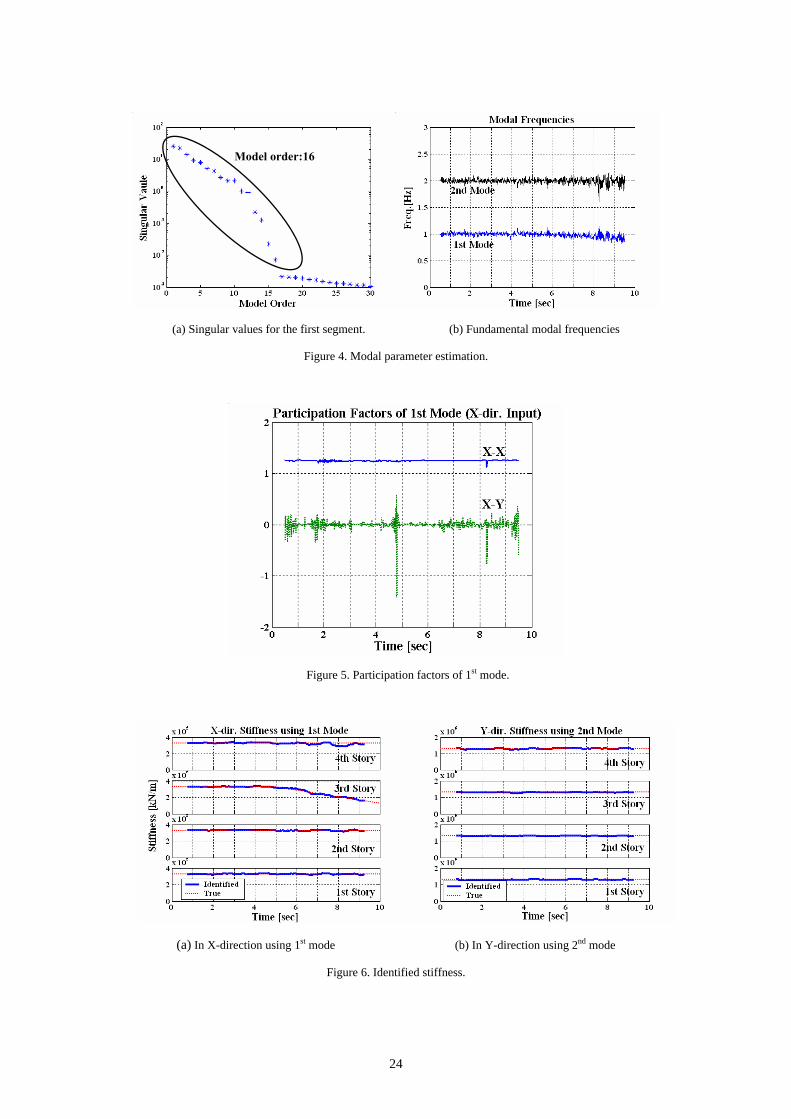
the first segment as shown in Figure 4(a), the model order was chosen to be 16. The

cumulative contribution ratio (the percentage of the sum of the selected singular values

to the whole singular values) of 16 singular values was retained more than 90% all the

time. In addition, we verified that the cumulative contribution factor is significantly

reduced when the sudden reduction of the story stiffness occurs in the model. This

means that the cumulative contribution ratio can be an index for detecting the change of

vibration characteristics due to the sudden destruction of the building. However,

detailed discussion on this matter is not included here.

Fundamental modal frequencies were estimated based on the lowest 2 poles as shown

in Figure 4(b). They correspond to the fundamental mode in X- and Y-direction,

respectively. But it is not obvious when the prior knowledge about the modal

information of the model was not available. To specify the input-output relationship in

the MIMO model, the participation factors are used. The time histories of the

15

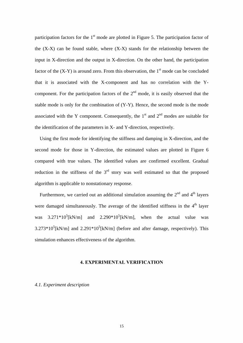
participation factors for the 1st mode are plotted in Figure 5. The participation factor of

the (X-X) can be found stable, where (X-X) stands for the relationship between the

input in X-direction and the output in X-direction. On the other hand, the participation

factor of the (X-Y) is around zero. From this observation, the 1st mode can be concluded

that it is associated with the X-component and has no correlation with the Y-

component. For the participation factors of the 2nd mode, it is easily observed that the

stable mode is only for the combination of (Y-Y). Hence, the second mode is the mode

associated with the Y component. Consequently, the 1st and 2nd modes are suitable for

the identification of the parameters in X- and Y-direction, respectively.

Using the first mode for identifying the stiffness and damping in X-direction, and the

second mode for those in Y-direction, the estimated values are plotted in Figure 6

compared with true values. The identified values are confirmed excellent. Gradual

reduction in the stiffness of the 3rd story was well estimated so that the proposed

algorithm is applicable to nonstationary response.

Furthermore, we carried out an additional simulation assuming the 2nd and 4th layers

were damaged simultaneously. The average of the identified stiffness in the 4th layer

was 3.271*105[kN/m] and 2.290*105[kN/m], when the actual value was

3.273*105[kN/m] and 2.291*105[kN/m] (before and after damage, respectively). This

simulation enhances effectiveness of the algorithm.

4. EXPERIMENTAL VERIFICATION

4.1. Experiment description

16

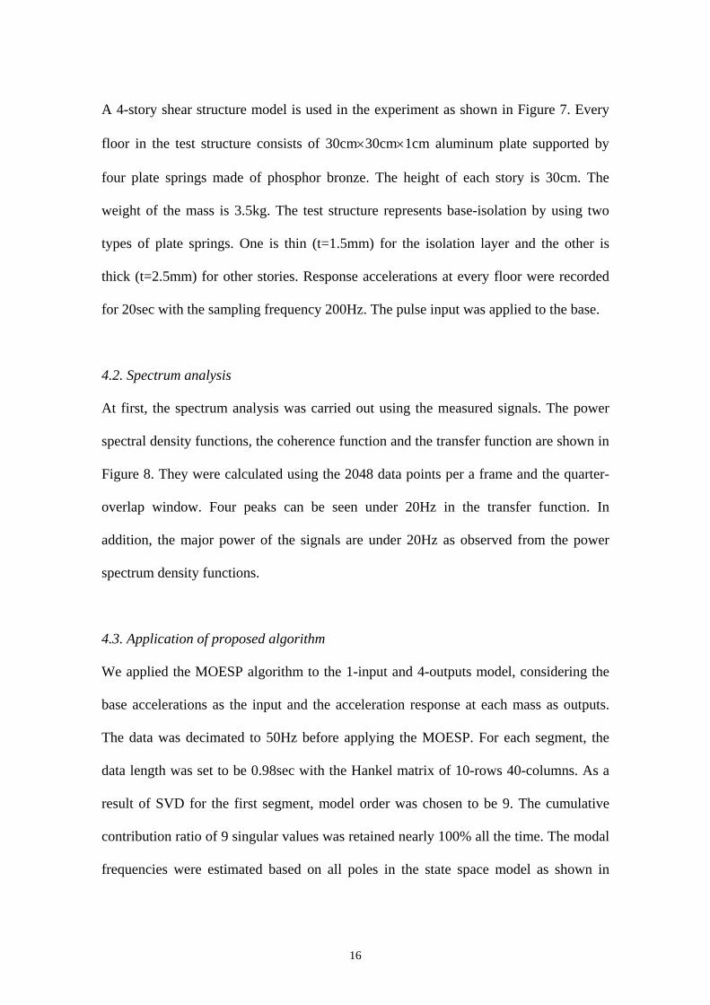
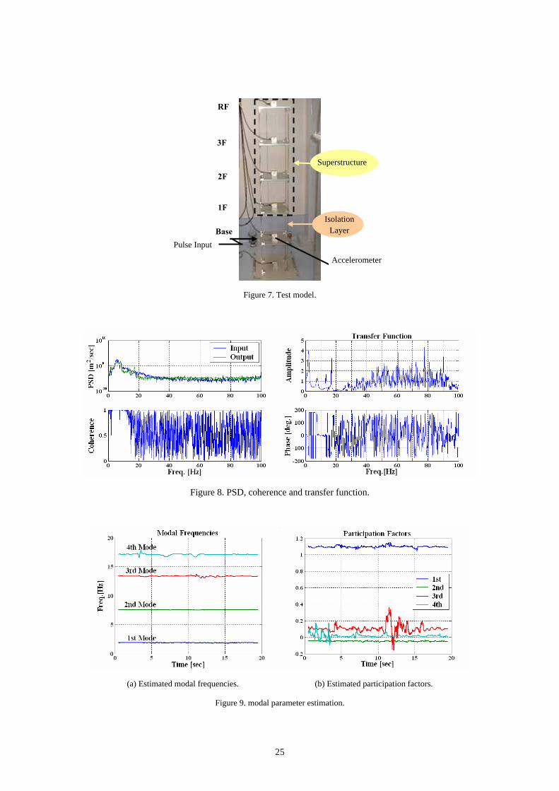
A 4-story shear structure model is used in the experiment as shown in Figure 7. Every

floor in the test structure consists of 30cm×30cm×1cm aluminum plate supported by

four plate springs made of phosphor bronze. The height of each story is 30cm. The

weight of the mass is 3.5kg. The test structure represents base-isolation by using two

types of plate springs. One is thin (t=1.5mm) for the isolation layer and the other is

thick (t=2.5mm) for other stories. Response accelerations at every floor were recorded

for 20sec with the sampling frequency 200Hz. The pulse input was applied to the base.

4.2. Spectrum analysis

At first, the spectrum analysis was carried out using the measured signals. The power

spectral density functions, the coherence function and the transfer function are shown in

Figure 8. They were calculated using the 2048 data points per a frame and the quarter-

overlap window. Four peaks can be seen under 20Hz in the transfer function. In

addition, the major power of the signals are under 20Hz as observed from the power

spectrum density functions.

4.3. Application of proposed algorithm

We applied the MOESP algorithm to the 1-input and 4-outputs model, considering the

base accelerations as the input and the acceleration response at each mass as outputs.

The data was decimated to 50Hz before applying the MOESP. For each segment, the

data length was set to be 0.98sec with the Hankel matrix of 10-rows 40-columns. As a

result of SVD for the first segment, model order was chosen to be 9. The cumulative

contribution ratio of 9 singular values was retained nearly 100% all the time. The modal

frequencies were estimated based on all poles in the state space model as shown in

17

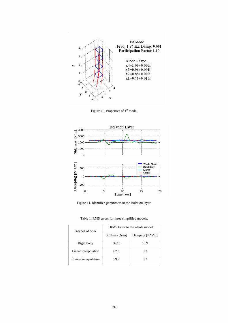
Figure 9(a). Comparing the participation factors as shown in Figure 9(b), the 1st mode

was found dominant and stable. Therefore, the 1st mode was chosen for estimating story

properties. The modal properties of the 1st mode are summarized in Figure 10.

Using the properties of the 1st mode, the stiffness and damping of the isolation layer

were identified. The results using three simple models are compared with the results

obtained by a whole model in Figure 11 and in Table 1. From the results, the cosine

interpolation showed the most accurate results. This observation is reasonable as the

mass and stiffness distribution for the model structure was uniform. In addition, the

simple hand calculation was carried out to compare the identified parameters with the

true parameters. Due to the simple hand calculation, the true stiffness in the isolation

layer is about 2000[N/m]. This is consistent with the identified value.

5. APPLICATION TO THE EXISTING BASE-ISOLATED BUILDING

5.1. Description of building and monitoring system

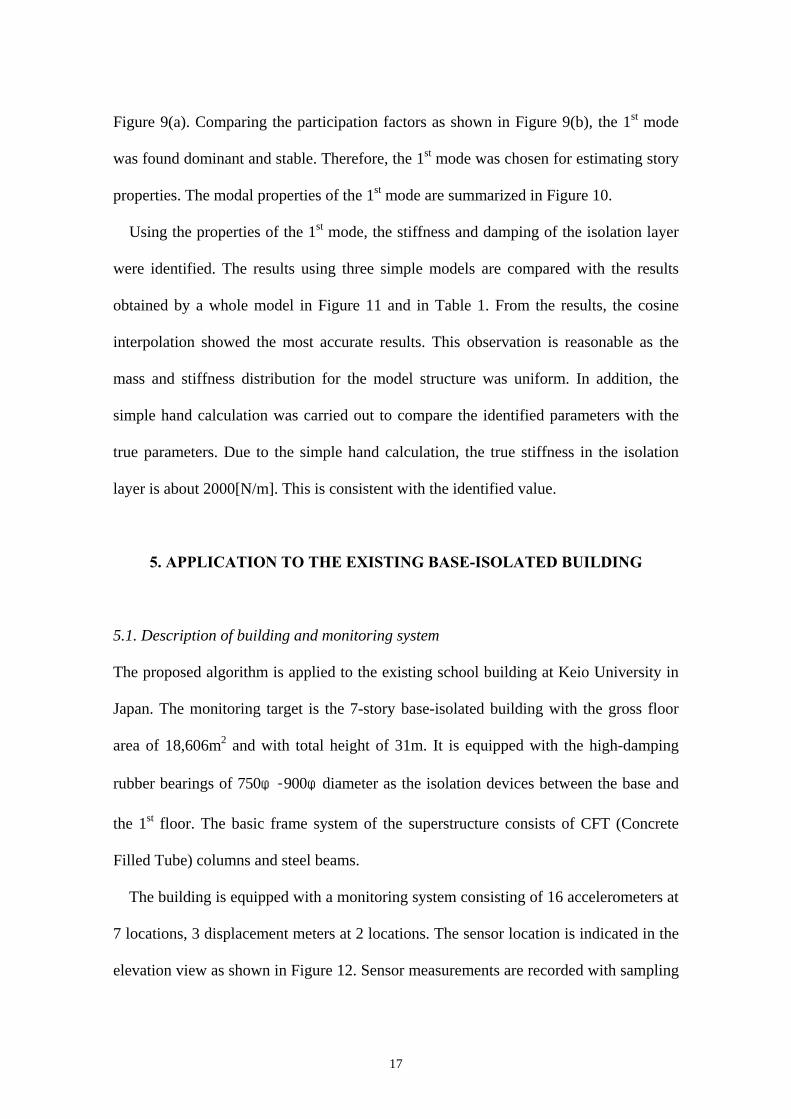
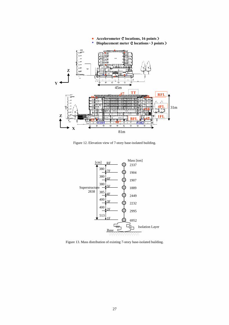
The proposed algorithm is applied to the existing school building at Keio University in

Japan. The monitoring target is the 7-story base-isolated building with the gross floor

area of 18,606m2 and with total height of 31m. It is equipped with the high-damping

rubber bearings of 750φ-900φdiameter as the isolation devices between the base and

the 1st floor. The basic frame system of the superstructure consists of CFT (Concrete

Filled Tube) columns and steel beams.

The building is equipped with a monitoring system consisting of 16 accelerometers at

7 locations, 3 displacement meters at 2 locations. The sensor location is indicated in the

elevation view as shown in Figure 12. Sensor measurements are recorded with sampling

18

frequency 100Hz in the monitoring server located on the 1st floor. The measured data

can be retrieved via internet. The web-server has several signal analysis tools so that

engineers can check the health of the building any time using his or her computer. For

conducting detailed analyses such as the one explained here, the stored data can be

easily downloaded to the local computer.

5.2. Analysis conditions

(1) The input-output data

In this analysis, 2-inputs and 6-outputs model was considered as summarized below:

Inputs: Translational acc. at the base ---- BF-Trans.X (#1-X) and BF-Trans.Y (#1-Y)

Outputs: Translational acc. in X-direction at the 1F and RF ---- RF-Trans.X (#5-X), 1F-

Trans.X (#2-X)

Translational acc. in Y-direction at the 1F and RF ---- RF-Trans.Y (#5-Y), 1F-

Trans.Y (#2-Y)

Torsional acc. at the 1F and RF ---- RF-Tors. [{(#5-Y)-(#6-Y)}/2], 1F-Tors.

[{(#2-Y)-(#3-Y)}/2]

(2) Prescribed model properties

The building is modeled as a lumped shear system. The mass distribution is given in

Figure 13.

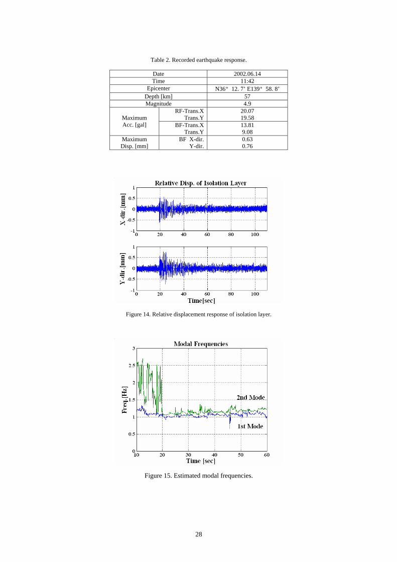
(3) Input earthquake

The small earthquake occurred in the southern area of Ibaraki prefecture in June 14,

2002 is used for the analysis. The characteristics of the earthquake are listed in Table 2.

19

The time histories of the relative displacement of the isolation layer are presented in

Figure 14 to show the level of the earthquake.

5.3 Evaluation of isolation layer

At first, data decimation to 20Hz was conducted. Then we estimated the modal

properties considering the 2-inputs and 6-outputs model as described in the previous

section. For each segment, the data length was set to be 3.95sec corresponding to the

Hankel matrix of 10-rows and 70-columns. As a result of SVD for the first segment,

model order was chosen to be 17. The cumulative contribution ratio of 17 singular

values was retained more than 90% all the time. Considering the response level, we

utilized data from 10 to 60sec in this analysis.

The lowest two modal frequencies were estimated as shown in Figure 15.

Considering the participation factors, the first mode was identified to be the

translational mode in Y-direction. Similarly, the second mode was identified to be the

translational mode in X-direction.

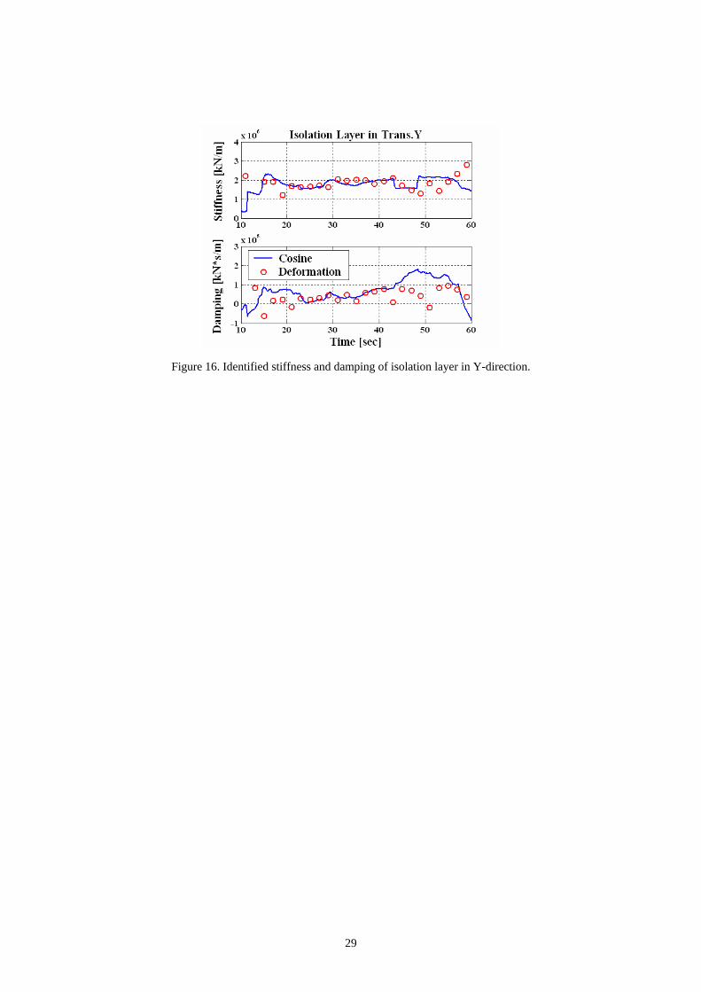
Therefore, the 1st mode is appropriate for identification of the parameters associated

with the Y-direction. The parameters in the isolation layer were identified using the

cosine interpolation and are shown in Figure 16 compared with the values calculated

from measured relative displacement data. Both results were found consistent, thus the

validity of our proposed method was confirmed. The identified stiffness in the isolation

layer, about 2*106kN/m, was in the same order of the story stiffness of the

superstructure. This means that the isolation devices were not in the operation range for

this small earthquake. The high-damping laminated rubber bearing is known that it

exhibits large variation in the damping values in the small amplitude vibration. For the

20

segments in which the amplitudes of response are small, the precise identification of

damping is difficult. Therefore, some values became negative.

6. CONCLUDING REMARKS

A damage detection algorithm for structural health monitoring systems based on the

subspace identification and the complex modal analysis was proposed. The proposed

algorithm is applicable to any shear structures. The algorithm utilizes the participation

factors to identify the input-output relations for each mode obtained from the MIMO

(Multi-Inputs and Multi-Outputs) models. Introducing the substructure approach, the

algorithm was tuned for base-isolated buildings so that the required number of sensors

would be significantly reduced. The effectiveness of the algorithm was examined

through the simulations and the experiments. Furthermore, applying the algorithm to the

existing 7-story base-isolated building that is equipped with an internet-based

monitoring system, feasibility of the algorithm was verified.

REFERENCES

1. Doebling W, Farrar R, Prime B, Shevitz W. Damage Identification and Health

Monitoring of Structural and Mechanical Systemes from Changes in their Vibration

Characteristics: a Literature Review. Los Alamos National Laboratory, 1996; 5-61.

2. Morita K, Teshigawara M, Isoda H, Hamamoto T, Mita A. Damage Detection Tests

of Five-Story Frame with Simulated Damages. Proceedings of the SPIE vol. 4335,

Advanced NDE Methods and Applications 2001.

21

3. Ko JM, Wong CW. Damage Detection in Steel Framed Structures by Vibration

Measurement Approach. Proceedings of 12th International Modal Analysis Conference

1994; 280-286.

4. Pandey AK. Damage detection from changes in curvature mode shapes. Journal of

Sound and Vibration 1991; 145(2):321-332.

5. Zang Z, Aktan AE. The Damage Indices for the Constructed Facilities. Proceedings

of the 13th International Modal Analysis Conference 1995; 1520-1529.

6. Loh CH, Tou IC. A system identification approach to detection of changes in both

linear and non-linear structural parameters. Earthquake Engineering and Structural

Dynamics 1995; 24:85-97.

7. Nakamura M, Takewaki I, Yasui Y, Uetani K. Simultaneous identification of

stiffness and damping of building structures using limited earthquake records. Journal

of Structural Construction Engineering 2000; 528:75-82, (in Japanese).

8. Mita A. Distributed health monitoring system for a tall building. Proceedings of 2nd

International Workshop on Structural Control 1996; 333-340.

9. Verhaegen M, Dewilde P. Subspace model identification part 1. The output-error

state-space model identification class of algorithms. International Journal of Control

1992; 56(5):1187-1210.

10. Juang JN, Pappa RS. An eigensystem realization algorithm for modal parameter

identification and model reduction. Journal of Guidance 1985; 8(5):620-627.

11. Juang JN. System Realization Using Information Matrix. Journal of Guidance

1997; 20(3):492-500.

12. Yoshimoto R, Mita A, Morita K. Parallel Identification of Structural Damages

Using Vibration Modes and Sensor Characteristics. Journal of Structural Engineering

22

2002; 48B:487-492, (in Japanese).

13. Skinner RI, Robinson WH, Mcverry GH. An Introduction to Seismic Isolation.

John Wiley & Sons, 1993.

14. Bathe KJ, Wilson EL. Numerical Methods in Finite Element Analysis. Prentice-

Hall, 1976; 319-322.

23

Figure 1. N-story shear structure.

(a) Rigid body (b) Linear interpolation (c) Cosine interpolation

Figure 2. Simplified models for base-isolated buildings.

Figure 3. 4-story shear model.

mN

mN-1

m2

m1

k1, c1

k2, c2

kN, cN

0X&&

1−NX&&

X-dir. Y-dir.

Mass: m1～m4=1000 [ton]

kx1=3.273×105

cx1=1.809×103

X-dir. Stiffness: [kN/m] X-dir. Damping: [kN*s/m]

kx2=3.273×105 cx2=1.809×103

kx3=3.273×105 →Gradual reduction cx3=1.809×103

kx4=3.273×105 cx4=1.809×103 ky4=1.309×106

cy4=1.809×103

ky3=1.309×106

cy3=1.809×103

ky2=1.309×106 cy2=1.809×103

ky1=1.309×106

cy1=1.809×103

Y-dir. Stiffness: [kN/m] Y-dir. Damping: [kN*s/m]

m4

m2

m3

m1

1X&&

NX&&

24

(a) Singular values for the first segment. (b) Fundamental modal frequencies

Figure 4. Modal parameter estimation.

Figure 5. Participation factors of 1st mode.

(a) In X-direction using 1st mode (b) In Y-direction using 2nd mode

Figure 6. Identified stiffness.

Model order:16

25

Figure 7. Test model.

Figure 8. PSD, coherence and transfer function.

(a) Estimated modal frequencies. (b) Estimated participation factors.

Figure 9. modal parameter estimation.

Pulse Input

Isolation Layer

Superstructure

Accelerometer

RF

3F

2F

1F

Base

26

Figure 10. Properties of 1st mode.

Figure 11. Identified parameters in the isolation layer.

Table 1. RMS errors for three simplified models.

RMS Error to the whole model3-types of SSA

Stiffness [N/m] Damping [N*s/m]

Rigid body 362.5 18.9

Linear interpolation 62.6 3.3

Cosine interpolation 59.9 3.3

27

● ●●

●

●●●

◆ ◆

Accelerometer（7 locations, 16 points）Displacement meter（2 locations、3 points）

●◆

X

Z

Y

Z

45m

81m

31m

RFL

4FL

1FLBFL

TT

#1#2#3

#4

#5#6#7

#102#103

●●●

●

● ●●

◆ ◆

Figure 12. Elevation view of 7-story base-isolated building.

Figure 13. Mass distribution of existing 7-story base-isolated building.

Mass [ton]2337

1904

1907

1889

2449

2232

2995

6952

RF

7F

6F

5F

4F

3F

2F

1F

2838

[cm]

380

380

380

385

400

400

513

Isolation LayerBase

Superstructure

28

Table 2. Recorded earthquake response.

Date 2002.06.14 Time 11:42

Epicenter N36°12. 7’ E139°58. 8’ Depth [km] 57 Magnitude 4.9

RF-Trans.XTrans.Y

20.07 19.58 Maximum

Acc. [gal] BF-Trans.XTrans.Y

13.81 9.08

Maximum Disp. [mm]

BF X-dir.Y-dir.

0.63 0.76

Figure 14. Relative displacement response of isolation layer.

Figure 15. Estimated modal frequencies.

29

Figure 16. Identified stiffness and damping of isolation layer in Y-direction.