Embed Size (px)
Citation preview
Daily Scheduling of Nurses in Operating Suites
Arezou MobasherDepartment of Industrial Engineering
The University of HoustonHouston, TX, [email protected]
Gino Lim1
Department of Industrial EngineeringThe University of Houston
Houston, TX, 77204713-743-4194
Jonathan F. BardGraduate Program in Operations Research
and Industrial EngineeringThe University of TexasAustin, TX 78712-0292
Victoria JordanQuality Engineering and Clinical Operations Informatics
The University of TexasMD Anderson Cancer CenterHouston, Texas [email protected]
1Corresponding author
Daily Scheduling of Nurses in Operating Suites
Abstract
This paper provides a new multi-objective integer programming model for the daily schedul-
ing of nurses in operating suites. The model is designed to assign nurses to different surgery cases
based on their specialties and competency levels, subject to a series of hard and soft constraints
related to nurse satisfaction, idle time, overtime, and job changes during a shift. To find solu-
tions, two methodologies were developed. The first is based on the idea of a solution pool and
the second is a variant of modified goal programming. The model and the solution procedures
were validated using real data provided by the University of Texas MD Anderson Cancer Center
in Houston, Texas. The results show that the two methodologies can produce schedules that
satisfy all demand with 50% less overtime and 50% less idle time when benchmarked against
current practice.
1 Introduction
The growing shortage of registered nurses continues to hamper the effective delivery of healthcare
throughout the United States and much of Europe (Ulrich et al., 2002). In a clinical setting,
not being able to assign a sufficient number of qualified nurses to a shift places undue stress on
those who are called upon to take up the slack. This, in turn, leads to reduced patient safety and
substandard treatment (Bester et al., 2007, Blythe et al., 2005, Cheng et al., 1997, Chiaramonte
and Chiaramonte, 2008). In the face of personnel shortages, hospital managers are under constant
pressure to balance the need to cover demand with the available staff, but without jeopardizing job
performance and satisfaction.
Assigning each available nurse to the right place at the right time to do the right job is a
major concern for healthcare organizations. As the types of services and treatments offered by
such organizations increase so do the skill requirements of their staff. In particular, nurses are
specifically trained and certified to work in a subset of units such as orthopedics or gerontology and
cannot be floated outside their areas of expertise. To make the most efficient use of the available
workforce then, it is necessary to adjust their schedules daily as the patient population changes.
When constructing individual schedules, one must consider the relevant skill categories, time-off
requests, shift preferences, demand variability by unit, break times and seniority, as well as system-
wide factors such as regulatory and union requirements, contractual agreements, and overtime. In
addition, each unit of a hospital may have a host of specific rules that further restrict the staffing
decisions. Although most of these rules are common throughout a hospital, there are a number
of exceptions, such as the way breaks are handled, when it comes to the operating suites, the
main focus of this paper. These exceptions further frustrate our ability to generate efficient daily
schedules.
An operating suite is an area in a hospital consisting of several operating rooms (ORs) where
surgical procedures are performed. Each OR is designed to accommodate specific types of surgeries
using specialized equipment. Because the operating suites are the largest revenue source in a
1
hospital (Belien and Demeulemeester, 2008) it is critical that they be scheduled to achieve maximum
utilization. Although we do not address this issue directly, it does have an impact on our research
since underutilized facilities may result in unnecessary nurse idle time, while overbooked ORs may
produce excessive overtime and high levels of staff dissatisfaction. When the prevailing nursing
shortage (Cardoen et al., 2010) is coupled with an increasing demand for surgeries linked to an
aging population, it is essential for hospital managers to maximize the use of their ORs and to
make the most efficient use of their nursing staff.
With this background in mind, the primary contribution of this research is the development of
a nurse scheduling tool designed to minimize overtime and idle time, delays due to staff shortages,
and assignment changes during the day, as well as to maximize case demand satisfaction. With
respect to the latter, it is critical to take into account nurse specialties and competency levels
along with various types of constraints such as shift limitations, contractual agreements and break
requirements when assigning them to cases. Considering the conflicting nature of these objectives
and insufficient resources to satisfy all constraints, it is not possible to identify and solve a single
optimization model. Instead, we attempt to create a pool of Pareto-optimal solutions such that
each optimizes at least one objective.
The rest of the paper is organized as follows. In Section 2 we provide a summary of the recent
nurse scheduling literature most relevant to our work. In Section 3 the planning environment is
outlined and a formal problem statement is given. In Section 4 we introduce our optimization model
for assigning nurses to surgery cases and, in Section 5, propose two competing solution algorithms
whose operations are described in detail. The first is based on the idea of a solution pool and the
second takes a modified goal programming approach. Numerical results are presented in Section
6 where it is shown that reductions in idle time and overtime of 50% or more are achievable with
respect to current practice. We close in Section 7 with several observations and suggestions for
future research. This work was done in conjunction with the University of Texas MD Anderson
Cancer Center (MDACC) who defined the problem and provided the test data.
2 Literature Review
Given the ever increasing labor costs in the healthcare industry and the fact that the nursing staff
accounts for approximately 50% of a hospital’s budget, a great deal of effort has been spent trying
to improve the nurse scheduling process (Ernst et al., 2004). Recent surveys include Cheang et al.
(2003) and Burke et al. (2004). With respect to the mid-term planning problem (up to 6 weeks),
integer programming (IP) methods have been widely used to either minimize cost or maximize
nurse preferences (Aickelin and Li, 2007, Bard and Purnomo, 2007, Ogulata et al., 2008). Others
have taken a heuristic approach including (Bai et al., 2010, Bard and Purnomo, 2007, Goodman
et al., 2009, He and Qu, 2009, Maenhout and Vanhoucke, 2010, Oddoye et al., 2006, Parr and
Thompson, 2007, Sundaramoorthi et al., 2009, Tsai and Li, 2009).
In contrast, there has been only a limited amount of research on the daily scheduling problem
which begins with the mid-term schedule and makes daily adjustments to account for changes in
2
demand, absenteeism, and skill mismatches (Burke et al., 2010, Hansen et al., 2010). Bard and
Purnomo (2005) formulated the problem as a mixed integer program and developed a branch-and-
price algorithm to find solutions. The objective was to minimize a combination staff dissatisfaction
costs due to preference violations and the cost of using agency nurses to cover shortages. The model
took a hospital-wide view and considered a float pool, overtime, and call-in nurses on their days
off. Optimal solutions for instances with up to 200 nurses were obtained using a rolling horizon
framework for each shift.
As mentioned in Section 1, due the importance of surgery and the unique teaming requirements
for each case, scheduling nurses in operating suites has been considered separately from scheduling
them in other areas of the hospital. Cardoen et al. (2010) provide a comprehensive review of recent
applications of operations research methods to operating room planning and scheduling. They
evaluated multiple domains related to problem settings, performance measures, solution methods
and uncertainty considerations. Much of the ongoing work is aimed at improving existing methods
to find the the best surgery-room assignments, surgery-physician assignments, and surgery-block
time assignments (Cardoen, 2010, Dexter et al., 1999, Ozkarahan, 2000).
Feia et al. (2008) developed an integer programming model for assigning surgical cases to several
multi-functional ORs with the objective of minimizing total operating cost. A branch-and-price
procedure was used to find solutions. The results were promising and showed that the approach
is capable of solving large instances In related work, Fei et al. (2009) addressed a tactical OR
planning problem and used a set-partitioning model to assign surgical cases to ORs one week at
a time. The assignments were based on an open scheduling strategy. Two conflicting objectives
were considered: maximize OR utilization and minimize overtime. To find solutions quickly, they
relied on a column generation based heuristic. Lamiri et al. (2008) proposed a stochastic model
for OR scheduling for both elective and emergency patients. The elective patients were assigned
to the different OR blocks depending on the type of surgery needed while emergency patients were
assigned to available time slots when they arrived at the facility. The objective was to minimize
related costs and overtime. The problem was formulated as a mixed integer program and solved with
a combination of optimization techniques and Monte Carlo simulation to deal with the uncertainty
of surgical durations and emergency arrivals.
Belien and Demeulemeester (2008) developed an integrated nurse and surgery scheduling system
for a weekly planning problem. The underlying model took the form of an integer program with
the objective of meeting nurse preferences while assuring that demand requirements were satisfied
in general, but not necessarily with respect to skill type. It was assumed that adequate resources
were available to cover all demand. The basic model was extended by enumerating all possible
ways of assigning operating blocks to the different surgeons subject to surgery demand and capacity
restrictions. A branch-and-price algorithm was proposed to find solutions. The pricing subproblems
used to generate columns for the master problem were solved with a standard dynamic program
and the results compared with those obtained with a commercial optimizer.
Although there exists a vast amount of literature on OR scheduling and nurse scheduling, there
has been little if any research on the problem of scheduling nurses in operating suites, even after the
3
surgeons and physicians have themselves been scheduled. Procedures for subsequently assigning
nurses are ad hoc, inefficient, and often give poor results. To the best of our knowledge, we are the
first to address this problem using an optimization approach.
3 Planning Environment and Problem Statement
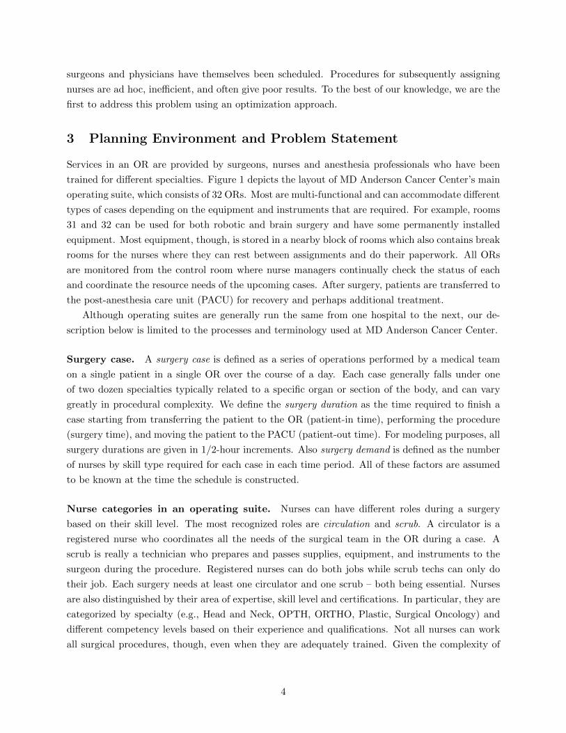
Services in an OR are provided by surgeons, nurses and anesthesia professionals who have been
trained for different specialties. Figure 1 depicts the layout of MD Anderson Cancer Center’s main
operating suite, which consists of 32 ORs. Most are multi-functional and can accommodate different
types of cases depending on the equipment and instruments that are required. For example, rooms
31 and 32 can be used for both robotic and brain surgery and have some permanently installed
equipment. Most equipment, though, is stored in a nearby block of rooms which also contains break
rooms for the nurses where they can rest between assignments and do their paperwork. All ORs
are monitored from the control room where nurse managers continually check the status of each
and coordinate the resource needs of the upcoming cases. After surgery, patients are transferred to
the post-anesthesia care unit (PACU) for recovery and perhaps additional treatment.
Although operating suites are generally run the same from one hospital to the next, our de-
scription below is limited to the processes and terminology used at MD Anderson Cancer Center.
Surgery case. A surgery case is defined as a series of operations performed by a medical team
on a single patient in a single OR over the course of a day. Each case generally falls under one
of two dozen specialties typically related to a specific organ or section of the body, and can vary
greatly in procedural complexity. We define the surgery duration as the time required to finish a
case starting from transferring the patient to the OR (patient-in time), performing the procedure
(surgery time), and moving the patient to the PACU (patient-out time). For modeling purposes, all
surgery durations are given in 1/2-hour increments. Also surgery demand is defined as the number
of nurses by skill type required for each case in each time period. All of these factors are assumed
to be known at the time the schedule is constructed.
Nurse categories in an operating suite. Nurses can have different roles during a surgery
based on their skill level. The most recognized roles are circulation and scrub. A circulator is a
registered nurse who coordinates all the needs of the surgical team in the OR during a case. A
scrub is really a technician who prepares and passes supplies, equipment, and instruments to the
surgeon during the procedure. Registered nurses can do both jobs while scrub techs can only do
their job. Each surgery needs at least one circulator and one scrub – both being essential. Nurses
are also distinguished by their area of expertise, skill level and certifications. In particular, they are
categorized by specialty (e.g., Head and Neck, OPTH, ORTHO, Plastic, Surgical Oncology) and
different competency levels based on their experience and qualifications. Not all nurses can work
all surgical procedures, though, even when they are adequately trained. Given the complexity of
4
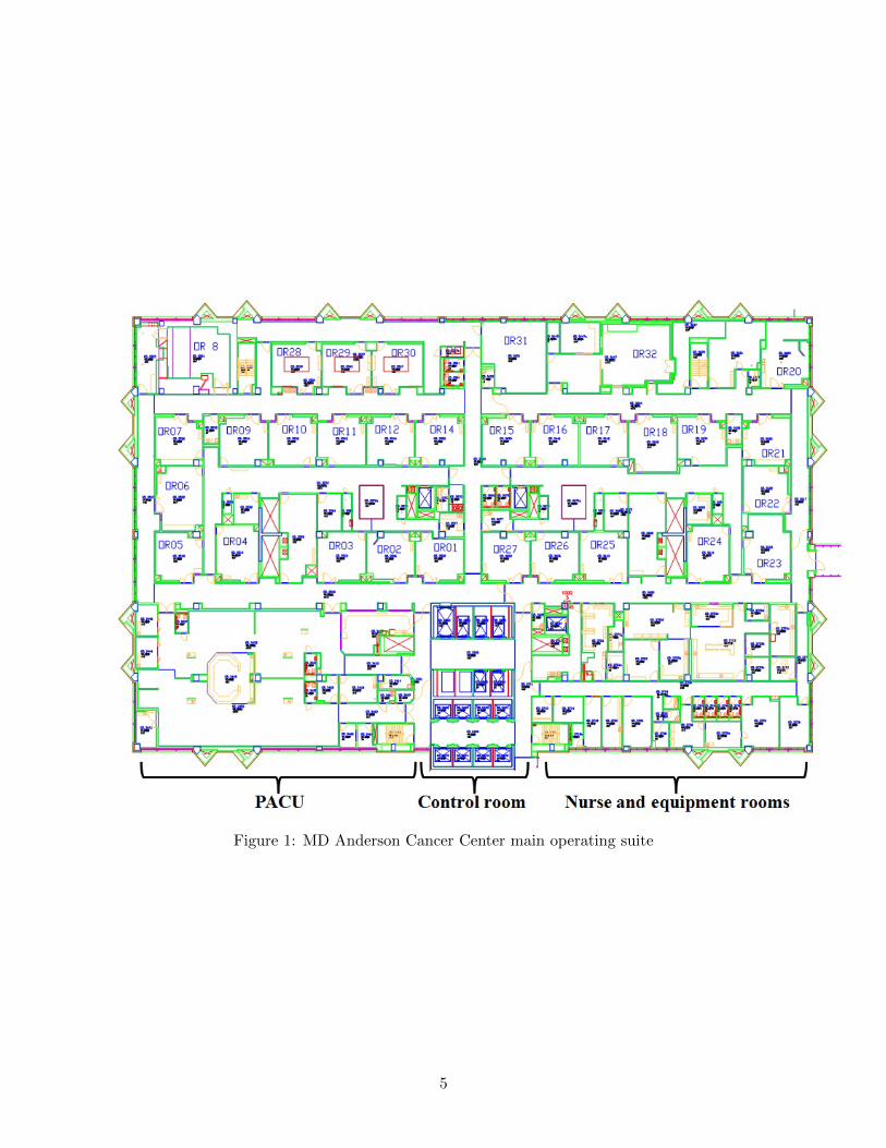
Figure 1: MD Anderson Cancer Center main operating suite
5
a procedure assignments are made based on the skill level and experience. Of course, nurses who
have enough experience to work on harder procedures can also work on easier ones.
Each day the scheduling department provides the nurse managers with the schedule sheets for
the next day. These sheets list the planned surgeries, the physician scheduled for each, his or her
instrument preferences, the room number, the estimated duration and procedural complexity, as
well as the nursing demand. From this information, the nurse managers construct and post the
case assignments for the nurses under their jurisdiction.
Shift limitations. Operating suites have shift restrictions along with regulatory and union re-
quirements similar to those imposed on the nurses in other areas of the hospital. We work with five
shift types defined by their length and starting time. All nurses upon being hired are assigned to
one of these shifts based on their contract. Each shift has its own lunch break and overtime rules.
During the scheduling process, available nurses are assigned to the various cases in accordance with
their qualifications and surgical needs. However, depending on the criticality of the surgery and the
condition of the patient, these rules can be overridden on a case-by-case basis. For instance, nurses
cannot leave a surgery to take a break unless the surgery is finished or someone else is available to
relieve them.
Given this environment, our aim is to develop a decision support tool that can be used by
nurse managers to assign nurses to surgery cases on a daily basis considering nurse availability,
shift restrictions, and demand requirements. It is assumed that complete information is available
on the number of nurses to be scheduled during each shift, their specialties and competencies, their
qualifications to assume certain roles, the surgery schedules and durations, case specialties and
procedural complexities, break requirements, and working contract options. The corresponding
parameter values are treated as inputs.
In next section, we present an integer programming model for making the daily nurse assign-
ments. As explained in Section 1, conflicting goals must be taken into account when deriving the
rosters so we chose not to optimize a single measure but instead to provide a set of high quality
solutions to the nurse managers. Then, by further taking into account fairness, seniority and related
issues, they can decide which assignments are “best” for their units. For comparative purposes, the
candidate schedules will be judged by staff utilization, the need for overtime, the degree to which
demand is met, and nurse satisfaction.
4 Nurse Assignment Model (NAM) - Problem Formulation
In formulating our integer programming model, it is necessary to take into account the special-
ties required for each case and the corresponding procedural complexities. As mentioned, nurses
have different competency levels and can only work on surgery cases that match their skills and
qualifications. In all, we wish to provide daily rosters that, to some extent balance five objectives
to be described presently. We start with the modeling assumptions and a series of hard and soft
6
constraints.
4.1 Assumptions and Notation
The operating suites run five days a week up to 17 hours per day. We assume that each working
day can be divided into a fixed number of time intervals of 30 minutes each, giving 38 planning
periods. Shifts are defined over 8- or 10-hour periods (not including a 1-hour lunch break) and have
different starting times. All shifts include regular hours and authorized overtime hours that bring
them up to 13 hours when lunch is included. Authorized overtime hours are additional hours that
a nurse can be assigned if a surgery is not finished by the end of her regular shift and either there
is no qualified nurse available to provide relief, or some in-progress cases have unfulfilled demand.
Note that all case durations are expressed in terms of the basic time interval.
Surgery complexity levels are classified as simple, moderate or complex. Nurses with a higher
competency can perform surgery procedures with lower complexity but not vice versa. If a nurse
is idle during a shift, it is assumed that she will be assigned to a surgery case as a learning fellow
(i.e., a nurse who is assigned to an OR room for the purpose of learning) in order to increase her
experience and competency. A final assumption is that each day is independent of another so a
daily decomposition is possible; that is, a separate model needs to be solved for each day rather
than for multiple days.
We start by introducing some basic notation in this and the next subsection.
C set of cases scheduled for surgery on the current day
H time intervals in a working day
I set of available nurses
J set of available ORs
K set of roles that are required for each surgery case
P set of competency/complexity levels (1: Simple, 2: Moderate, 3: Complex)
Q set of specialties
S set of available shifts
T nurse job category(1 = RN, 2 = scrub tech)
4.2 Input Parameters
The constraints in our model are a function of ten parameters that are defined below. Parameters P1
and P2 respectively specify the shift that each nurse works, the role, specialty and competency level
of that nurse, and her job category. The next five parameters P3, P4, P5, P6 and P7 characterize the
surgery cases and their attributes. They provide information about each case duration, specialty
7

and procedural complexity, number of required nurses in each role, and the time intervals in which
each is performed. Finally, parameters P8 and P9 indicate the starting time of each shift, the
regular hours of the shift and authorized overtime hours.
d2ick 1 if nurse i is assigned to case c to do job k, and 0 otherwise
P 1is 1 if nurse i ∈ I is working in shift s ∈ S, 0 otherwise
P 2ikqp 1 if nurse i ∈ I can do role k ∈ K in specialty q ∈ Q with competency level p ∈ P, 0
otherwise
P 3cj 1 if case c ∈ C is scheduled to happen in OR j ∈ J , 0 otherwise
P 4cqph 1 if case c ∈ C needs specialty q ∈ Q and has procedural complexity p ∈ P in time interval
h ∈ H, 0 otherwise
P 5ckh required number of nurses for case c ∈ C who can perform role k ∈ K in time interval h ∈ H
P 6ch 1 if case c ∈ C is in progress during time interval h ∈ H, 0 otherwise
P 7c case c ∈ C duration (length of surgery)
P 8sh 1 if shift s ∈ S contains time interval h ∈ H as regular working hours, 0 otherwise
P 9sh 1 if shift s ∈ S contains time interval h ∈ H as authorized overtime hours, 0 otherwise
M big number estimated from other parameter values
4.3 Decision Variables
Our aim is to determine which nurse should be assigned to which surgery case, during which time
intervals, and what their role should be. The corresponding decision variable is:
yickh =
1, if nurse i ∈ I works on case c ∈ C in time interval h ∈ H doing role k ∈ K
0, otherwise
4.4 Constraints
The constraints listed in this section are applicable for all nurses without considering break hours.
They are divided into two sets. The first set corresponds to those constraints that must be satisfied
(hard) and the second to those that may be violated but at a cost (soft). The latter are related to
our various objective functions and are referred to as objective constraints.
8

Hard constraints. These constraints cannot be violated under any circumstances, and concern
shift restrictions, nurse skill levels, and case requirements, to name a few. Although some nurses
are qualified to work in different roles, each nurse must be assigned to one case in each time interval
to perform one specific job. During a shift, each nurse can be given at most 8 regular hours of
work and 4 overtime hours, or 10 regular hours and 2 overtime hours. Nurses must be assigned to
surgery cases based on their specialties and competency levels.
∑c∈C
∑k∈K
yickh ≤ 1, i ∈ I, h ∈ H (1)
yickh ≤∑s∈S
(P 1is · (P 8
sh + P 9sh)), i ∈ I, c ∈ C, k ∈ K, h ∈ H (2)∑
c∈C
∑k∈K
∑h∈H
yickh ≤∑s∈S
∑h∈H
(P 1is · (P 8
sh + P 9sh)), i ∈ I (3)
yickh ≤ P 6ch ·
∑q∈Q,
∑p∈P
(P 4cqph · P 2
ikqp
), i ∈ I, c ∈ C, k ∈ K, h ∈ H (4)
∑i∈I
yickh ≥ P 6ch, c ∈ C, k ∈ K, h ∈ H (5)∑
h∈Hyickh ≤M · d2ick, i ∈ I, c ∈ C, k ∈ K (6)∑
k∈Kd2ick ≤ 1, i ∈ I, c ∈ C (7)
Constraints (1) limit the number of cases and roles that nurse i can be assigned in time interval
h to at most 1. Constraints (2) and (3) ensure that nurses will only be assigned to cases that are
in progress during their shift s, and that the total working hours scheduled will be less than or
equal to the total number of regular and overtime hours associated with s. Constraints (4) and (5)
ensure that, if a case is in progress, a nurse can only be assigned to it if she has the requisite skills
and competency to deal with its procedural complexities.
It is preferred that nurses be scheduled to work continuously during their shift and perform the
same job for the duration of each surgery to which they are assigned, rather than alternate between
jobs. This is enforced with constraints (6) and (7.
The latter constraints restricts the maximum number of times that a nurse can be assigned to
serve in different roles during a specific case and it is at most 1.
Soft (objective) constraints. These constraints need not be satisfied exactly but penalties will
be imposed to minimize the magnitude of their violations. Demand satisfaction, room assignments
and job changes are considered as objective constraints. Each surgery must be assigned at least one
circulator and one scrub, but it may be desirable to include more in each category. Under staffing
represents our first permissible deviation that is penalized. In a similar vein, mismatches between
supply and demand can lead to a need for overtime, job changes, room changes or excessive breaks
9

during a shift. The corresponding deviations will also be penalized. With respect to the individual
nurses, we wish to minimize (i) the number of breaks in a shift, (ii) the amount of overtime assigned,
(iii) the number of different cases assigned, (iv) the number of job changes, (v) and the number of
breaks over the day. Nurses prefer to work continuously during their shifts and perform the same
role, at least for a given surgery, rather than move from one case to another.
To formulate these goals as soft constraints, we define a pair of deviation variables for each;
that is,
deckh 1 if there is a deviation in demand in case c ∈ C for job k ∈ K in time interval h ∈ H, 0
otherwise
DE maximum demand deviation for any case c ∈ C and job k ∈ K
d7ih 1 if nurse i ∈ I is idle in time interval h ∈ H, 0 otherwise
DS maximum number of nonconsecutive idle intervals for any nurse i ∈ I
d4ih 1 if nurse i ∈ I is assigned overtime in time interval h ∈ H, 0 otherwise
DF maximum amount of overtime assigned to any nurse i ∈ I
xij 1 if nurse i ∈ I is assigned to room j ∈ J , 0 otherwise
X maximum number of room assignments for any nurse i ∈ I
ncic 1 if nurse i ∈ I is assigned to case c ∈ C, 0 otherwise
cdic 1 if the assignment of nurse i ∈ I to case c ∈ C is broken, 0 otherwise
NCT maximum number of case assignments given to any nurse i ∈ I
CDT maximum number of times an individual assignment to a case is broken due to shortages
for any nurse i ∈ I
Based on these definitions, the soft constraints can be stated as follows.∑i∈I
yickh + deckh ≥ P 5ckh · P 6
ch, c ∈ C, k ∈ K, h ∈ H (8)
DE ≥∑h∈H
deckh, c ∈ C, k ∈ K (9)
∣∣∣∣∣∑c∈C
∑k∈K
yick(h+1) −∑c∈C
∑k∈K
yickh
∣∣∣∣∣ ≤ d7ih, i ∈ I, h ∈ H (10)
DS ≥∑h∈H
d7ih, i ∈ I, (11)
10
∑c∈C
∑k∈K
∑h∈H
(P 3cj · yickh
)≤M · xij , i ∈ I, j ∈ J (12)
X ≥∑j∈J
xij , i ∈ I (13)
d4ih −∑s∈S
P 1is · P 9
sh ·∑c∈C
∑k∈K
yickh ≥ 0, i ∈ I, h ∈ H (14)
DF ≥∑h∈H
d4ih, i ∈ I (15)
∑k∈K
∑h∈H
yickh −∑h∈H
P 6ch +M · cdic +M · (1− ncic) ≥ 0, i ∈ I, c ∈ C (16)
∑k∈K
∑h∈H
yickh ≤M · ncic, i ∈ I, c ∈ C (17)
NCT ≥∑c∈C
ncic, i ∈ I (18)
CDT ≥∑c∈C
cdic. i ∈ I (19)
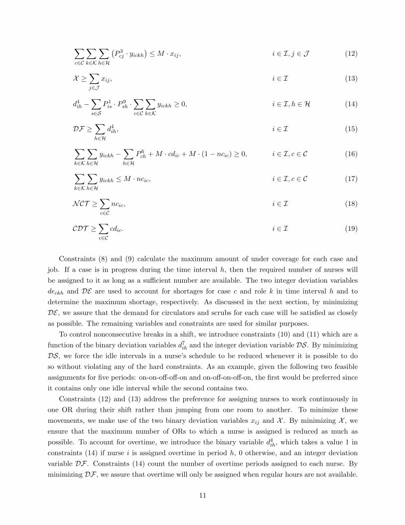
Constraints (8) and (9) calculate the maximum amount of under coverage for each case and
job. If a case is in progress during the time interval h, then the required number of nurses will
be assigned to it as long as a sufficient number are available. The two integer deviation variables
deckh and DE are used to account for shortages for case c and role k in time interval h and to
determine the maximum shortage, respectively. As discussed in the next section, by minimizing
DE , we assure that the demand for circulators and scrubs for each case will be satisfied as closely
as possible. The remaining variables and constraints are used for similar purposes.
To control nonconsecutive breaks in a shift, we introduce constraints (10) and (11) which are a
function of the binary deviation variables d7ih and the integer deviation variable DS. By minimizing
DS, we force the idle intervals in a nurse’s schedule to be reduced whenever it is possible to do
so without violating any of the hard constraints. As an example, given the following two feasible
assignments for five periods: on-on-off-off-on and on-off-on-off-on, the first would be preferred since
it contains only one idle interval while the second contains two.
Constraints (12) and (13) address the preference for assigning nurses to work continuously in
one OR during their shift rather than jumping from one room to another. To minimize these
movements, we make use of the two binary deviation variables xij and X . By minimizing X , we
ensure that the maximum number of ORs to which a nurse is assigned is reduced as much as
possible. To account for overtime, we introduce the binary variable d4ih, which takes a value 1 in
constraints (14) if nurse i is assigned overtime in period h, 0 otherwise, and an integer deviation
variable DF . Constraints (14) count the number of overtime periods assigned to each nurse. By
minimizing DF , we assure that overtime will only be assigned when regular hours are not available.
11
Finally, constraints (16), (17), (18) and (19) with deviation variables ncic, cdic, NCT and CDTassure that if a nurse is assigned to a case, it will be for its entire duration unless staffing shortages
dictate that she be reassigned elsewhere to avoid violating a hard constraint. Also, by minimizing
the maximum number of cases that a nurse can work, we limit her movement from period to period.
4.5 Objective Function
As implied in the above discussion, we wish to minimize six conflicting objectives. Each corresponds
to a maximum deviation from a stated goal. In particular, the objective of NAM is to minimize:
DE maximum demand deviation for any case c ∈ C and job k ∈ K
DS maximum number of nonconsecutive breaks for any nurse i ∈ I
DF maximum amount of overtime assigned to any nurse i ∈ I
X maximum number of room assignments to any nurse i ∈ I
NCT maximum number of cases assigned to any nurse i ∈ I
CDT maximum number of times an individual assignment to a case is broken due to shortages
for any nurse i ∈ I
The corresponding objective function can be written as
Minimize [DE ,DF ,DS,X ,NCT , CDT ] (20)
and is designed to ensure that the maximum deviation for each goal (worst case results) will be
minimized for all nurses and cases.
5 Solution Methods
A variety of solution techniques are available to deal with the multi-objective nature of the nurse
assignment model. One of the most common is to construct a single objective function by weighting
each term (deviation) and summing them. This was the first scheme we tried but were unable to get
optimal solutions with CPLEX after 10 hours of computations. Nevertheless, we make use of this
idea indirectly in one of our two proposed methods. The first is based on the idea of constructing
a pool of high quality solutions; the second makes use of goal programming techniques (e.g., see
Schniederjans, 1995). Each is described in the remainder of this section.
5.1 Solution Pool Approach
Rather than terminate with an “optimal” solution to an optimization problem, several of the more
powerful commercial codes offer a feature that accumulates feasible solutions in a pool. CPLEX,
for example, now has the option to save a specified number of solutions that are within a given
12
percentage of the optimum (IBM, 2010). In our first approach to the NAM, called SPM, we use
this feature in CPLEX to generate a set of candidate rosters which are then evaluated with respect
to the six objectives. The methodology is outlined in Algorithm 1 and consists of three steps. In
Step 1, all input data sets, parameters and goals are initialized, and an index j is assigned to each
variable contained in (20). In Step 2, we solve a single objective problem for each deviation. All
hard constraints as well as those soft constraints associated with the current deviation are included.
For example, for the the first deviation DE , the problem is:
Minimize DEsubject to hard constraints: (1)− (7)
soft constraints: (8)− (9)
(21)
The solution pool feature is applied to this problem to generate S candidates, and the process
repeated for the remaining deviations. Since soft constraints do not affect feasibility, regardless of
the objective function in model (21), all the feasible regions contain the same hard constraints so
a feasible solution with objective j will also be feasible for objective j′ ∈ {1, . . . , J} \ {j}. Thus,
given a solution s for objective j, we can calculate the objective values associated with the other
deviation j′ at s. To be able to compare different candidates, we also calculate a cumulative weighted
index CWIjs for each solution s ∈ {1, . . . , S} and objective j ∈ {1, . . . , J}. The weights used in
forming the index are based on the decision maker’s perceived importance of each deviation. The
comparisons are performed in Step 3 and the candidate that yields the smallest CWI is reported
as the NAM solution.
Upon termination, the value of the decision variables Y ∗j∗s∗
ickh associated with CWI∗ are reported
as the solution, where CWI∗ is the smallest cumulative weighted index found at Step 3. The values
of the six deviations are also reported.
Example 1. To illustrate the approach, suppose that we have a problem with three deviations
defined in terms of the goals g1, g2 and g3, a set of hard constraints Ax ≤ B, and a pair of soft
constraints for each deviation j given by Cj(x) ≤ Dj , where, goal gj(x) is associated with constraint
Cj(x) ≤ Dj for j = 1, 2, 3. The corresponding multi-objective optimization model can be stated as
follows.
Minimize z1 = g1(x)
Minimize z2 = g2(x)
Minimize z3 = g3(x)
subject to Ax ≤ BCj(x) ≤ Dj ∀ j = 1, 2, 3
x ∈ Z+
(23)
For each j, the single objective model is
13
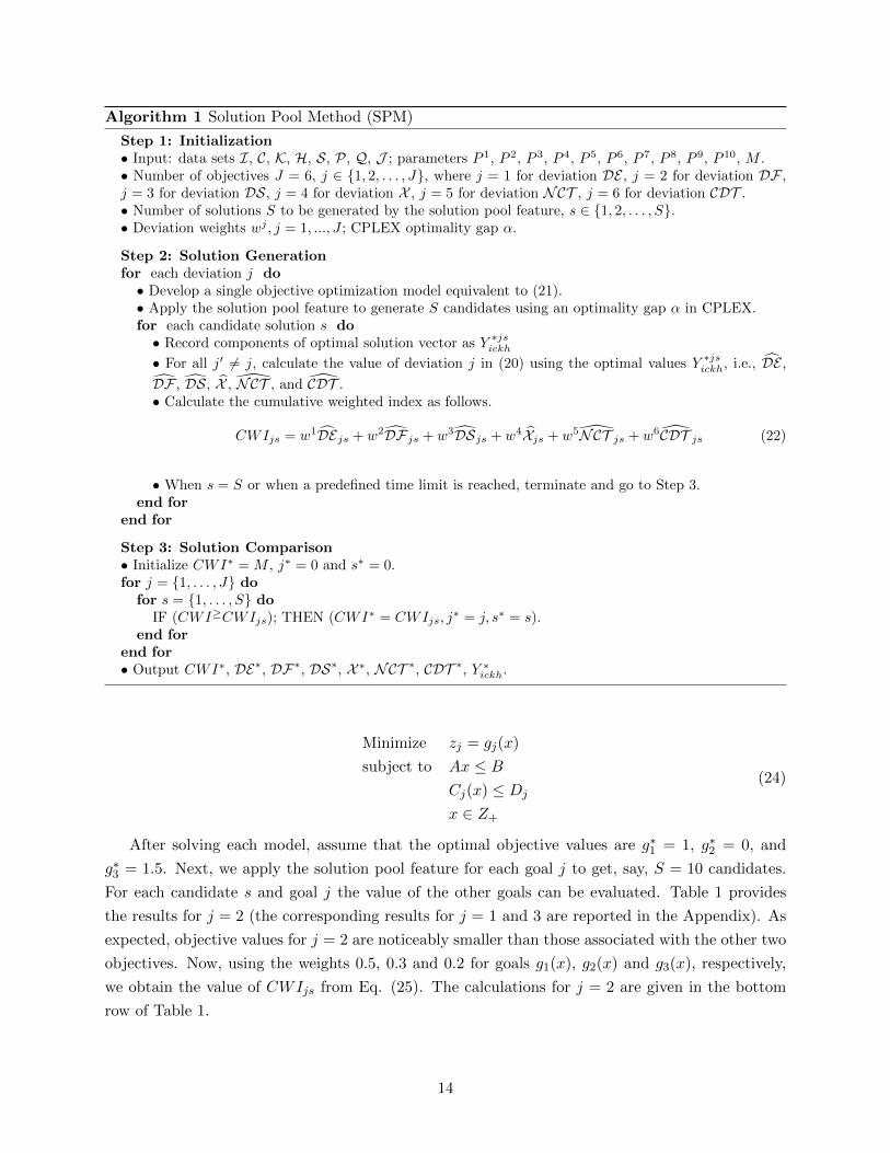
Algorithm 1 Solution Pool Method (SPM)
Step 1: Initialization• Input: data sets I, C, K, H, S, P, Q, J ; parameters P 1, P 2, P 3, P 4, P 5, P 6, P 7, P 8, P 9, P 10, M .• Number of objectives J = 6, j ∈ {1, 2, . . . , J}, where j = 1 for deviation DE , j = 2 for deviation DF ,j = 3 for deviation DS, j = 4 for deviation X , j = 5 for deviation NCT , j = 6 for deviation CDT .• Number of solutions S to be generated by the solution pool feature, s ∈ {1, 2, . . . , S}.• Deviation weights wj , j = 1, ..., J ; CPLEX optimality gap α.
Step 2: Solution Generationfor each deviation j do• Develop a single objective optimization model equivalent to (21).• Apply the solution pool feature to generate S candidates using an optimality gap α in CPLEX.for each candidate solution s do• Record components of optimal solution vector as Y ∗jsickh
• For all j′ 6= j, calculate the value of deviation j in (20) using the optimal values Y ∗jsickh, i.e., DE ,
DF , DS, X , N CT , and CDT .• Calculate the cumulative weighted index as follows.
CWIjs = w1DEjs + w2DFjs + w3DSjs + w4Xjs + w5N CT js + w6CDT js (22)
• When s = S or when a predefined time limit is reached, terminate and go to Step 3.end for
end for
Step 3: Solution Comparison• Initialize CWI∗ = M , j∗ = 0 and s∗ = 0.for j = {1, . . . , J} do
for s = {1, . . . , S} doIF (CWI≥CWIjs); THEN (CWI∗ = CWIjs, j
∗ = j, s∗ = s).end for
end for• Output CWI∗, DE∗, DF∗, DS∗, X ∗, NCT ∗, CDT ∗, Y ∗ickh.
Minimize zj = gj(x)
subject to Ax ≤ BCj(x) ≤ Dj
x ∈ Z+
(24)
After solving each model, assume that the optimal objective values are g∗1 = 1, g∗2 = 0, and
g∗3 = 1.5. Next, we apply the solution pool feature for each goal j to get, say, S = 10 candidates.
For each candidate s and goal j the value of the other goals can be evaluated. Table 1 provides
the results for j = 2 (the corresponding results for j = 1 and 3 are reported in the Appendix). As
expected, objective values for j = 2 are noticeably smaller than those associated with the other two
objectives. Now, using the weights 0.5, 0.3 and 0.2 for goals g1(x), g2(x) and g3(x), respectively,
we obtain the value of CWIjs from Eq. (25). The calculations for j = 2 are given in the bottom
row of Table 1.
14
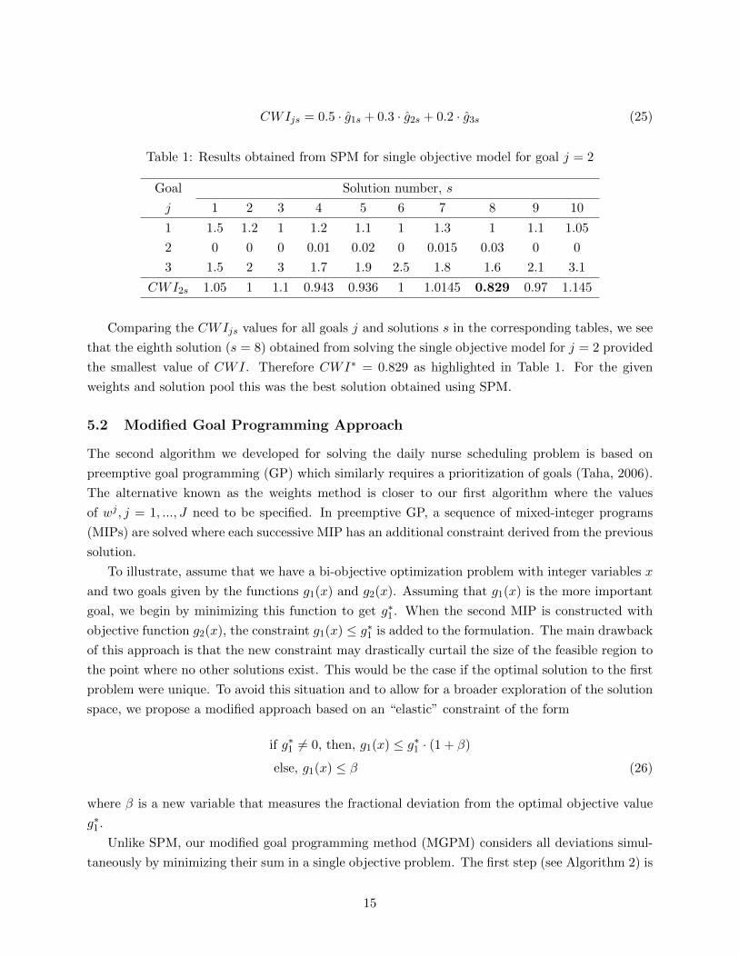
CWIjs = 0.5 · g1s + 0.3 · g2s + 0.2 · g3s (25)
Table 1: Results obtained from SPM for single objective model for goal j = 2
Goal Solution number, s
j 1 2 3 4 5 6 7 8 9 10
1 1.5 1.2 1 1.2 1.1 1 1.3 1 1.1 1.05
2 0 0 0 0.01 0.02 0 0.015 0.03 0 0
3 1.5 2 3 1.7 1.9 2.5 1.8 1.6 2.1 3.1
CWI2s 1.05 1 1.1 0.943 0.936 1 1.0145 0.829 0.97 1.145
Comparing the CWIjs values for all goals j and solutions s in the corresponding tables, we see
that the eighth solution (s = 8) obtained from solving the single objective model for j = 2 provided
the smallest value of CWI. Therefore CWI∗ = 0.829 as highlighted in Table 1. For the given
weights and solution pool this was the best solution obtained using SPM.
5.2 Modified Goal Programming Approach
The second algorithm we developed for solving the daily nurse scheduling problem is based on
preemptive goal programming (GP) which similarly requires a prioritization of goals (Taha, 2006).
The alternative known as the weights method is closer to our first algorithm where the values
of wj , j = 1, ..., J need to be specified. In preemptive GP, a sequence of mixed-integer programs
(MIPs) are solved where each successive MIP has an additional constraint derived from the previous
solution.
To illustrate, assume that we have a bi-objective optimization problem with integer variables x
and two goals given by the functions g1(x) and g2(x). Assuming that g1(x) is the more important
goal, we begin by minimizing this function to get g∗1. When the second MIP is constructed with
objective function g2(x), the constraint g1(x) ≤ g∗1 is added to the formulation. The main drawback
of this approach is that the new constraint may drastically curtail the size of the feasible region to
the point where no other solutions exist. This would be the case if the optimal solution to the first
problem were unique. To avoid this situation and to allow for a broader exploration of the solution
space, we propose a modified approach based on an “elastic” constraint of the form
if g∗1 6= 0, then, g1(x) ≤ g∗1 · (1 + β)
else, g1(x) ≤ β (26)
where β is a new variable that measures the fractional deviation from the optimal objective value
g∗1.
Unlike SPM, our modified goal programming method (MGPM) considers all deviations simul-
taneously by minimizing their sum in a single objective problem. The first step (see Algorithm 2) is
15
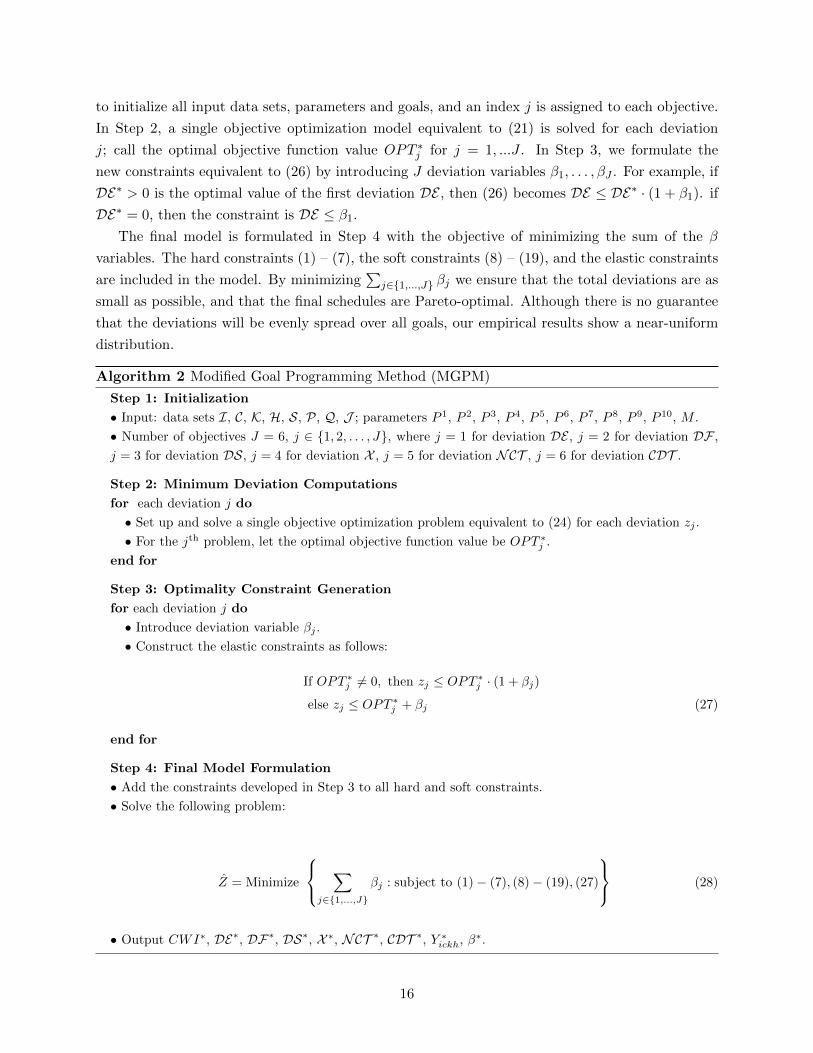
to initialize all input data sets, parameters and goals, and an index j is assigned to each objective.
In Step 2, a single objective optimization model equivalent to (21) is solved for each deviation
j; call the optimal objective function value OPT ∗j for j = 1, ...J . In Step 3, we formulate the
new constraints equivalent to (26) by introducing J deviation variables β1, . . . , βJ . For example, if
DE∗ > 0 is the optimal value of the first deviation DE , then (26) becomes DE ≤ DE∗ · (1 + β1). if
DE∗ = 0, then the constraint is DE ≤ β1.The final model is formulated in Step 4 with the objective of minimizing the sum of the β
variables. The hard constraints (1) – (7), the soft constraints (8) – (19), and the elastic constraints
are included in the model. By minimizing∑
j∈{1,...,J} βj we ensure that the total deviations are as
small as possible, and that the final schedules are Pareto-optimal. Although there is no guarantee
that the deviations will be evenly spread over all goals, our empirical results show a near-uniform
distribution.
Algorithm 2 Modified Goal Programming Method (MGPM)
Step 1: Initialization
• Input: data sets I, C, K, H, S, P, Q, J ; parameters P 1, P 2, P 3, P 4, P 5, P 6, P 7, P 8, P 9, P 10, M .
• Number of objectives J = 6, j ∈ {1, 2, . . . , J}, where j = 1 for deviation DE , j = 2 for deviation DF ,
j = 3 for deviation DS, j = 4 for deviation X , j = 5 for deviation NCT , j = 6 for deviation CDT .
Step 2: Minimum Deviation Computations
for each deviation j do
• Set up and solve a single objective optimization problem equivalent to (24) for each deviation zj .
• For the jth problem, let the optimal objective function value be OPT ∗j .
end for
Step 3: Optimality Constraint Generation
for each deviation j do
• Introduce deviation variable βj .
• Construct the elastic constraints as follows:
If OPT ∗j 6= 0, then zj ≤ OPT ∗j · (1 + βj)
else zj ≤ OPT ∗j + βj (27)
end for
Step 4: Final Model Formulation
• Add the constraints developed in Step 3 to all hard and soft constraints.
• Solve the following problem:
Z = Minimize
∑j∈{1,...,J}
βj : subject to (1)− (7), (8)− (19), (27)
(28)
• Output CWI∗, DE∗, DF∗, DS∗, X ∗, NCT ∗, CDT ∗, Y ∗ickh, β∗.
16
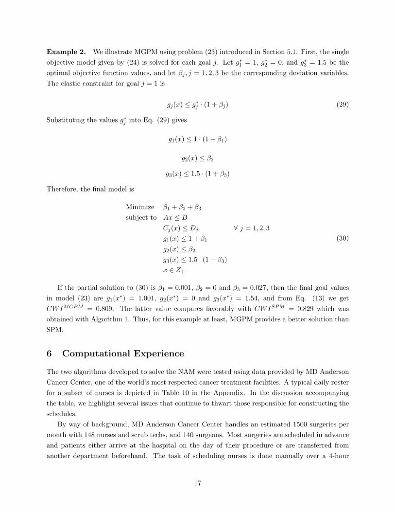
Example 2. We illustrate MGPM using problem (23) introduced in Section 5.1. First, the single
objective model given by (24) is solved for each goal j. Let g∗1 = 1, g∗2 = 0, and g∗3 = 1.5 be the
optimal objective function values, and let βj , j = 1, 2, 3 be the corresponding deviation variables.
The elastic constraint for goal j = 1 is
gj(x) ≤ g∗j · (1 + βj) (29)
Substituting the values g∗j into Eq. (29) gives
g1(x) ≤ 1 · (1 + β1)
g2(x) ≤ β2
g3(x) ≤ 1.5 · (1 + β3)
Therefore, the final model is
Minimize β1 + β2 + β3
subject to Ax ≤ BCj(x) ≤ Dj ∀ j = 1, 2, 3
g1(x) ≤ 1 + β1
g2(x) ≤ β2g3(x) ≤ 1.5 · (1 + β3)
x ∈ Z+
(30)
If the partial solution to (30) is β1 = 0.001, β2 = 0 and β3 = 0.027, then the final goal values
in model (23) are g1(x∗) = 1.001, g2(x
∗) = 0 and g3(x∗) = 1.54, and from Eq. (13) we get
CWIMGPM = 0.809. The latter value compares favorably with CWISPM = 0.829 which was
obtained with Algorithm 1. Thus, for this example at least, MGPM provides a better solution than
SPM.
6 Computational Experience
The two algorithms developed to solve the NAM were tested using data provided by MD Anderson
Cancer Center, one of the world’s most respected cancer treatment facilities. A typical daily roster
for a subset of nurses is depicted in Table 10 in the Appendix. In the discussion accompanying
the table, we highlight several issues that continue to thwart those responsible for constructing the
schedules.
By way of background, MD Anderson Cancer Center handles an estimated 1500 surgeries per
month with 148 nurses and scrub techs, and 140 surgeons. Most surgeries are scheduled in advance
and patients either arrive at the hospital on the day of their procedure or are transferred from
another department beforehand. The task of scheduling nurses is done manually over a 4-hour
17
period from 3 PM to 7 PM the day before with the actual assignments being finalized on the
current day. Call-ins, cancellations, overtime and case-duration variability make the problem even
more complex and frustrating.
On average, 60 nurses with RN and scrub tech titles are available a various times during the
day, depending on their contractual agreements. The following five different shifts are used in the
operating suites, each spanning either 8 or 10 regular hours plus overtime and lunch.
Shift 1: 6:30 AM - 2:30 PM (8 regular hours, 4 overtime hours, 1 hour for lunch)
Shift 2: 6:30 AM - 5:30 PM (10 regular hours, 4 overtime hours, 1 hour for lunch)
Shift 3: 10:30 AM - 5:30 PM (8 regular hours, 4 overtime hours, 1 hour for lunch)
Shift 4: 10:30 AM - 7:30 PM (10 regular hours, 2 overtime hours, 1 hour for lunch)
Shift 5: 2:30 PM - 11:30 PM (8 regular hours, 4 overtime hours, 0 hours for lunch)
To construct a problem instance, we collected surgery case data and nurse attribute data for
one day in May and one day in November 2010 for the main operating suite. These data, in
collaboration with several nurse managers, allowed us to define all model parameters and preference
settings. Input information included nurse specialties and competency levels, their shifts and job
titles, case specialties, procedural complexities, and demand per case. The basic data set was built
around 28 cases to be staffed by 23 RNs and 14 scrubs each working one of the five shifts defined
above. The demand for each case was 1 circulator and 1 scrub. For modeling purposes, the day
was broken into 38 half-hour time periods starting at 6:30 AM and ending at 11:30 PM. Both
algorithms were implemented in a C++ environment and run under Windows Server 2008 R2 on a
2.83 GHz Dell workstation with 16 GB of memory. All integer programs were solved with CPLEX
12.2.
6.1 Results for Solution Pool Method
To evaluate the performance of SPM we conducted four experiments using the different weight
values shown in Table 2. Experiment 1 assigns equal weight to all six deviations. The remainder
reflect the preferences of the various nurse managers at MD Anderson Cancer Center. In all cases,
surgery demand satisfaction (DE) was deemed to be of highest importance. In Experiment 2, less
preference is given to overtime (DF) and nonconsecutive assignments (DS) than to moving between
cases (NCT ) and unfinished surgery assignments (CDT ). The third and fourth experiments can
be similarly interpreted.
18
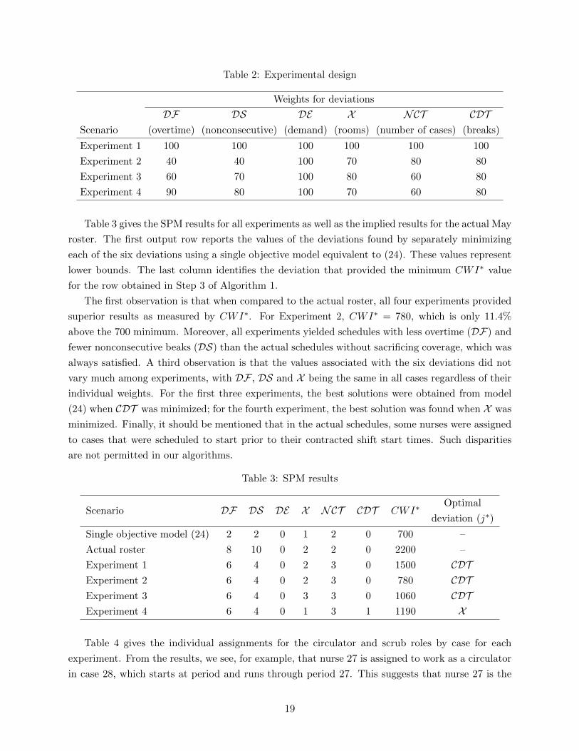
Table 2: Experimental design
Weights for deviations
DF DS DE X NCT CDTScenario (overtime) (nonconsecutive) (demand) (rooms) (number of cases) (breaks)
Experiment 1 100 100 100 100 100 100
Experiment 2 40 40 100 70 80 80
Experiment 3 60 70 100 80 60 80
Experiment 4 90 80 100 70 60 80
Table 3 gives the SPM results for all experiments as well as the implied results for the actual May
roster. The first output row reports the values of the deviations found by separately minimizing
each of the six deviations using a single objective model equivalent to (24). These values represent
lower bounds. The last column identifies the deviation that provided the minimum CWI∗ value
for the row obtained in Step 3 of Algorithm 1.
The first observation is that when compared to the actual roster, all four experiments provided
superior results as measured by CWI∗. For Experiment 2, CWI∗ = 780, which is only 11.4%
above the 700 minimum. Moreover, all experiments yielded schedules with less overtime (DF) and
fewer nonconsecutive beaks (DS) than the actual schedules without sacrificing coverage, which was
always satisfied. A third observation is that the values associated with the six deviations did not
vary much among experiments, with DF , DS and X being the same in all cases regardless of their
individual weights. For the first three experiments, the best solutions were obtained from model
(24) when CDT was minimized; for the fourth experiment, the best solution was found when X was
minimized. Finally, it should be mentioned that in the actual schedules, some nurses were assigned
to cases that were scheduled to start prior to their contracted shift start times. Such disparities
are not permitted in our algorithms.
Table 3: SPM results
Scenario DF DS DE X NCT CDT CWI∗Optimal
deviation (j∗)
Single objective model (24) 2 2 0 1 2 0 700 –
Actual roster 8 10 0 2 2 0 2200 –
Experiment 1 6 4 0 2 3 0 1500 CDTExperiment 2 6 4 0 2 3 0 780 CDTExperiment 3 6 4 0 3 3 0 1060 CDTExperiment 4 6 4 0 1 3 1 1190 X
Table 4 gives the individual assignments for the circulator and scrub roles by case for each
experiment. From the results, we see, for example, that nurse 27 is assigned to work as a circulator
in case 28, which starts at period and runs through period 27. This suggests that nurse 27 is the
19
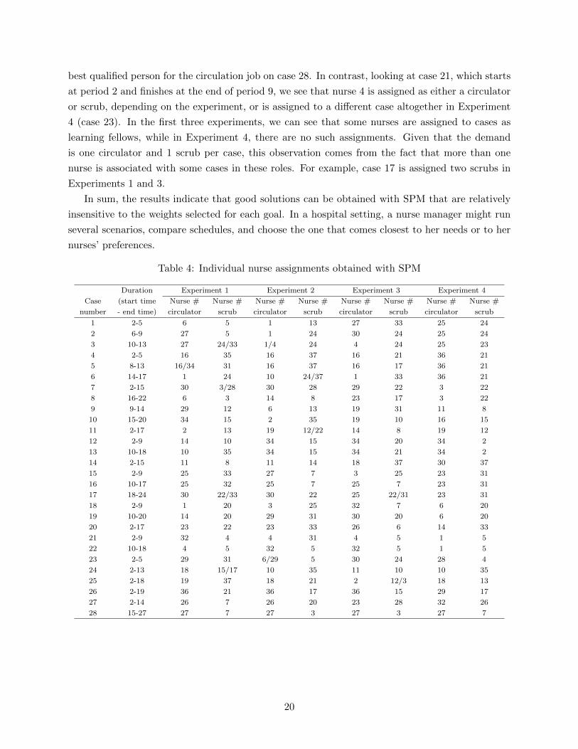
best qualified person for the circulation job on case 28. In contrast, looking at case 21, which starts
at period 2 and finishes at the end of period 9, we see that nurse 4 is assigned as either a circulator
or scrub, depending on the experiment, or is assigned to a different case altogether in Experiment
4 (case 23). In the first three experiments, we can see that some nurses are assigned to cases as
learning fellows, while in Experiment 4, there are no such assignments. Given that the demand
is one circulator and 1 scrub per case, this observation comes from the fact that more than one
nurse is associated with some cases in these roles. For example, case 17 is assigned two scrubs in
Experiments 1 and 3.
In sum, the results indicate that good solutions can be obtained with SPM that are relatively
insensitive to the weights selected for each goal. In a hospital setting, a nurse manager might run
several scenarios, compare schedules, and choose the one that comes closest to her needs or to her
nurses’ preferences.
Table 4: Individual nurse assignments obtained with SPM
Duration Experiment 1 Experiment 2 Experiment 3 Experiment 4
Case (start time Nurse # Nurse # Nurse # Nurse # Nurse # Nurse # Nurse # Nurse #
number - end time) circulator scrub circulator scrub circulator scrub circulator scrub
1 2-5 6 5 1 13 27 33 25 24
2 6-9 27 5 1 24 30 24 25 24
3 10-13 27 24/33 1/4 24 4 24 25 23
4 2-5 16 35 16 37 16 21 36 21
5 8-13 16/34 31 16 37 16 17 36 21
6 14-17 1 24 10 24/37 1 33 36 21
7 2-15 30 3/28 30 28 29 22 3 22
8 16-22 6 3 14 8 23 17 3 22
9 9-14 29 12 6 13 19 31 11 8
10 15-20 34 15 2 35 19 10 16 15
11 2-17 2 13 19 12/22 14 8 19 12
12 2-9 14 10 34 15 34 20 34 2
13 10-18 10 35 34 15 34 21 34 2
14 2-15 11 8 11 14 18 37 30 37
15 2-9 25 33 27 7 3 25 23 31
16 10-17 25 32 25 7 25 7 23 31
17 18-24 30 22/33 30 22 25 22/31 23 31
18 2-9 1 20 3 25 32 7 6 20
19 10-20 14 20 29 31 30 20 6 20
20 2-17 23 22 23 33 26 6 14 33
21 2-9 32 4 4 31 4 5 1 5
22 10-18 4 5 32 5 32 5 1 5
23 2-5 29 31 6/29 5 30 24 28 4
24 2-13 18 15/17 10 35 11 10 10 35
25 2-18 19 37 18 21 2 12/3 18 13
26 2-19 36 21 36 17 36 15 29 17
27 2-14 26 7 26 20 23 28 32 26
28 15-27 27 7 27 3 27 3 27 7
20
6.2 Results for Modified Goal Programming Method
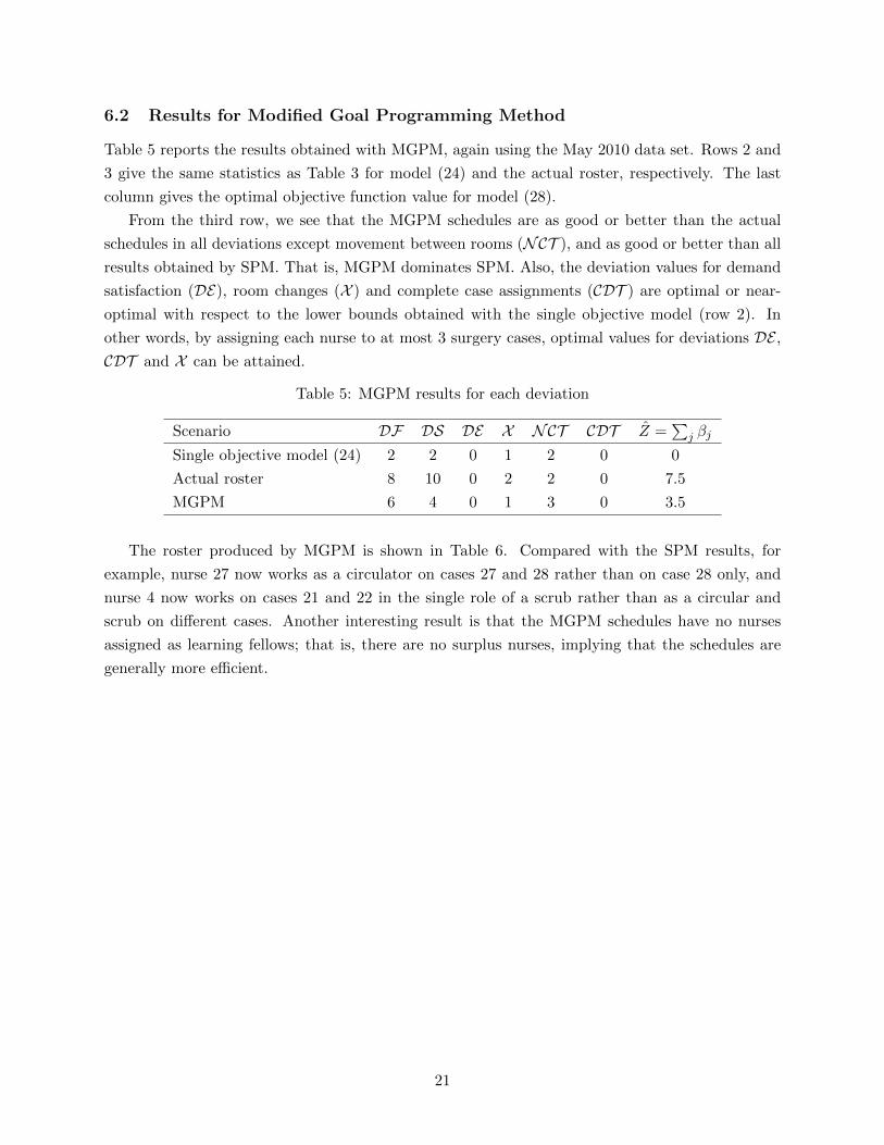
Table 5 reports the results obtained with MGPM, again using the May 2010 data set. Rows 2 and
3 give the same statistics as Table 3 for model (24) and the actual roster, respectively. The last
column gives the optimal objective function value for model (28).
From the third row, we see that the MGPM schedules are as good or better than the actual
schedules in all deviations except movement between rooms (NCT ), and as good or better than all
results obtained by SPM. That is, MGPM dominates SPM. Also, the deviation values for demand
satisfaction (DE), room changes (X ) and complete case assignments (CDT ) are optimal or near-
optimal with respect to the lower bounds obtained with the single objective model (row 2). In
other words, by assigning each nurse to at most 3 surgery cases, optimal values for deviations DE ,
CDT and X can be attained.
Table 5: MGPM results for each deviation
Scenario DF DS DE X NCT CDT Z =∑
j βj
Single objective model (24) 2 2 0 1 2 0 0
Actual roster 8 10 0 2 2 0 7.5
MGPM 6 4 0 1 3 0 3.5
The roster produced by MGPM is shown in Table 6. Compared with the SPM results, for
example, nurse 27 now works as a circulator on cases 27 and 28 rather than on case 28 only, and
nurse 4 now works on cases 21 and 22 in the single role of a scrub rather than as a circular and
scrub on different cases. Another interesting result is that the MGPM schedules have no nurses
assigned as learning fellows; that is, there are no surplus nurses, implying that the schedules are
generally more efficient.
21
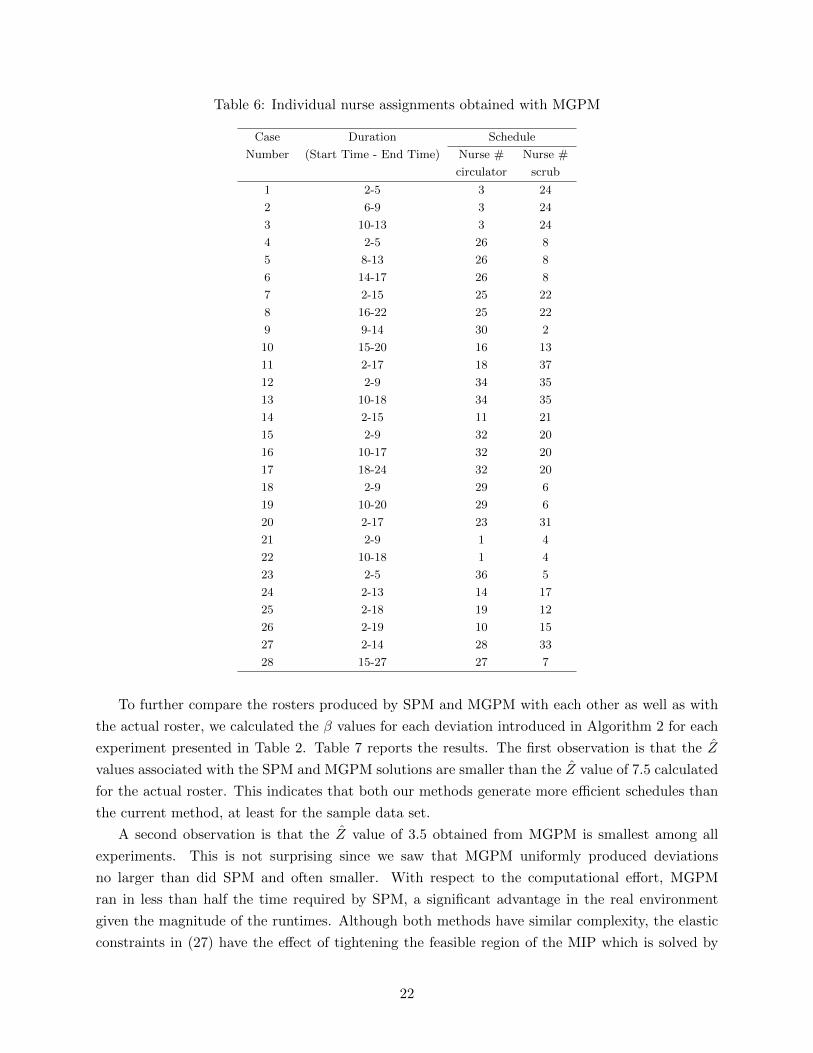
Table 6: Individual nurse assignments obtained with MGPM
Case Duration Schedule
Number (Start Time - End Time) Nurse # Nurse #
circulator scrub
1 2-5 3 24
2 6-9 3 24
3 10-13 3 24
4 2-5 26 8
5 8-13 26 8
6 14-17 26 8
7 2-15 25 22
8 16-22 25 22
9 9-14 30 2
10 15-20 16 13
11 2-17 18 37
12 2-9 34 35
13 10-18 34 35
14 2-15 11 21
15 2-9 32 20
16 10-17 32 20
17 18-24 32 20
18 2-9 29 6
19 10-20 29 6
20 2-17 23 31
21 2-9 1 4
22 10-18 1 4
23 2-5 36 5
24 2-13 14 17
25 2-18 19 12
26 2-19 10 15
27 2-14 28 33
28 15-27 27 7
To further compare the rosters produced by SPM and MGPM with each other as well as with
the actual roster, we calculated the β values for each deviation introduced in Algorithm 2 for each
experiment presented in Table 2. Table 7 reports the results. The first observation is that the Z
values associated with the SPM and MGPM solutions are smaller than the Z value of 7.5 calculated
for the actual roster. This indicates that both our methods generate more efficient schedules than
the current method, at least for the sample data set.
A second observation is that the Z value of 3.5 obtained from MGPM is smallest among all
experiments. This is not surprising since we saw that MGPM uniformly produced deviations
no larger than did SPM and often smaller. With respect to the computational effort, MGPM
ran in less than half the time required by SPM, a significant advantage in the real environment
given the magnitude of the runtimes. Although both methods have similar complexity, the elastic
constraints in (27) have the effect of tightening the feasible region of the MIP which is solved by
22
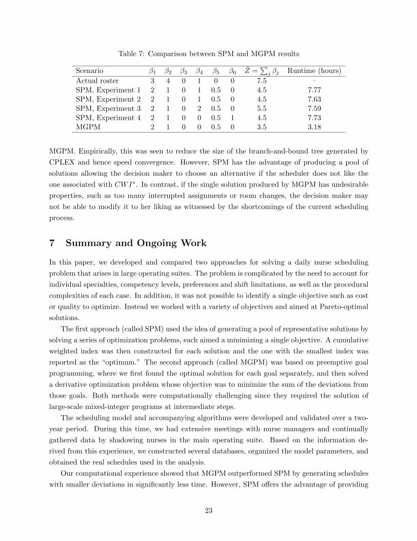
Table 7: Comparison between SPM and MGPM results
Scenario β1 β2 β3 β4 β5 β6 Z =∑
j βj Runtime (hours)
Actual roster 3 4 0 1 0 0 7.5 –SPM, Experiment 1 2 1 0 1 0.5 0 4.5 7.77SPM, Experiment 2 2 1 0 1 0.5 0 4.5 7.63SPM, Experiment 3 2 1 0 2 0.5 0 5.5 7.59SPM, Experiment 4 2 1 0 0 0.5 1 4.5 7.73MGPM 2 1 0 0 0.5 0 3.5 3.18
MGPM. Empirically, this was seen to reduce the size of the branch-and-bound tree generated by
CPLEX and hence speed convergence. However, SPM has the advantage of producing a pool of
solutions allowing the decision maker to choose an alternative if the scheduler does not like the
one associated with CWI∗. In contrast, if the single solution produced by MGPM has undesirable
properties, such as too many interrupted assignments or room changes, the decision maker may
not be able to modify it to her liking as witnessed by the shortcomings of the current scheduling
process.
7 Summary and Ongoing Work
In this paper, we developed and compared two approaches for solving a daily nurse scheduling
problem that arises in large operating suites. The problem is complicated by the need to account for
individual specialties, competency levels, preferences and shift limitations, as well as the procedural
complexities of each case. In addition, it was not possible to identify a single objective such as cost
or quality to optimize. Instead we worked with a variety of objectives and aimed at Pareto-optimal
solutions.
The first approach (called SPM) used the idea of generating a pool of representative solutions by
solving a series of optimization problems, each aimed a minimizing a single objective. A cumulative
weighted index was then constructed for each solution and the one with the smallest index was
reported as the “optimum.” The second approach (called MGPM) was based on preemptive goal
programming, where we first found the optimal solution for each goal separately, and then solved
a derivative optimization problem whose objective was to minimize the sum of the deviations from
those goals. Both methods were computationally challenging since they required the solution of
large-scale mixed-integer programs at intermediate steps.
The scheduling model and accompanying algorithms were developed and validated over a two-
year period. During this time, we had extensive meetings with nurse managers and continually
gathered data by shadowing nurses in the main operating suite. Based on the information de-
rived from this experience, we constructed several databases, organized the model parameters, and
obtained the real schedules used in the analysis.
Our computational experience showed that MGPM outperformed SPM by generating schedules
with smaller deviations in significantly less time. However, SPM offers the advantage of providing
23

many good solutions from which the decision maker can choose, based on her individual preferences
or perceptions of fairness that might not have been captured in the models. It is an easy matter
to rank the solutions in the pool or filter out those that do not meet certain implicit goals. It
is also simple to re-rank them by adjusting the weights used to compute CWI. In any case, the
results from either model proved superior to those obtained with the current techniques in use at
MD Anderson Cancer Center so it is anticipated that the implementation of either of approach will
lead to measurable savings in the coming years.
Nevertheless, the numerical results showed that neither algorithm could provide solutions quickly,
so developing more efficient computational methods would be valuable. We are currently looking
into the use of column generation to get improved relaxed solutions and heuristics for converting
them to feasible solutions. We believe that this approach will lead to at least a twofold reduction
in runtimes.
One of the main characteristics of any OR is case continuity. A nurse cannot leave the OR
until the case is finished or she is relieved by someone with comparable qualifications. In practice,
this means that there must be a pool of nurses on call, so to speak, during a portion of the day to
take over when a lunch break is requested. We are now developing a complementary optimization
model to generate lunch schedules for those shifts that require a break. Upon completion, we
expect to wrap all the models with a graphical user interface that will facilitate daily planning, OR
monitoring, and real-time control. When nurses call out or surgeries extend beyond their planned
durations, a user friendly system is needed to get the schedules and cases back on track.
References
U. Aickelin and J. Li. An estimation of distribution algorithm for nurse scheduling. Annals of
Operation Research, 155(1):289–309, 2007.
R. Bai, E. Burke, G. Kendall, J. Li, and G. McCollum. A hybrid evolutionary approach to the
nurse rostering problem. IEEE Transactions on Evolutionary Computation, 14(4):580–590, 2010.
J. Bard and H. Purnomo. Hospital-wide reactive scheduling of nurses with preference considerations.
IIE Transactions, 37(7):589–608, 2005.
J. Bard and H. Purnomo. Cyclic preference scheduling of nurses using a Lagrangian-based heuristic.
Journal of Scheduling, 10(1):5–23, 2007.
J. Belien and E. Demeulemeester. A branch-and-price approach for integrating nurse and surgery
scheduling. European Journal of Operational Research, 189(3):652–668, 2008.
M. Bester, I. Nieuwoudt, and J. Van Vuuren. Finding good nurse duty schedules: a case study.
Journal of Scheduling, 10(6):387–405, 2007.
J. Blythe, A. Baumann, I. Zeytinoglu, M. Denton, and A. Higgins. Full-time or part-time work in
nursing: preferences, Trade-offs and choices. Healthcare Quarterly, 8(3):69–77, 2005.
24
E. Burke, P. De Causmaecker, and H. Van Landeghem. The state of the art of nurse rostering.
Journal of Scheduling, 7(6):441–499, 2004.
E. Burke, J. Li, and R. Qu. A hybrid model of integer programming and variable neighborhood
search for highly-constrained nurse rostering problems. European Journal of Operational Re-
search, 203(2):484–493, 2010.
B. Cardoen. Operating room planning and scheduling: solving a surgical case sequencing problem.
A Quarterly Journal of Operations Research, 8(1):101–104, 2010.
B. Cardoen, E. Demeulemeester, and J. Belien. Operating room planning and scheduling: a liter-
ature review. European Journal of Operational Research, 201(3):921–932, 2010.
B. Cheang, H. Li, A. Lim, and B. Rodrigues. Nurse rostering problems, a bibliographic survey.
European Journal of Operational Research, 151(3):447–460, 2003.
B. Cheng, J. Lee, and J. Wu. A constraint-based nurse rostering system using a redundant modeling
approach. Information Technology in Biomedicine, 1(1):44–54, 1997.
M. Chiaramonte and L. Chiaramonte. An agent-based nurse rostering system under minimal staffing
conditions. International Journal of Production Economics, 114(2):697–713, 2008.
F. Dexter, A. Macario, R. Traub, M. Hopwood, and D. Lubarsky. An operating room scheduling
strategy to maximize the use of operating room block time: computer simulation of patient
scheduling and survey of patients preferences for surgical waiting time. Economics and Health
Systems Research, 89(1):7, 1999.
A. Ernst, H. Jiang, M. Krishnamoorthy, B. Owens, and D. Sier. An annotated bibliography of
personnel scheduling and rostering. Annals of Operations Research, 127(1):21–144, 2004.
H. Fei, C. Chu, and N. Meskens. Solving a tactical operating room planning problem by a column-
generation-based heuristic procedure with four criteria. Annals of Operations Research, 166(1):
91–108, 2009.
H. Feia, C. Chub, N. Meskensa, and A. Artiba. Solving surgical cases assignment problem by a
branch-and-price approach. Journal of Production Economics, 112(1):96–108, 2008.
M. Goodman, K. Dowsland, and J. Thompson. A grasp-knapsack hybrid for a nurse scheduling
problem. Journal of Heuristics, 15(4):351–379, 2009.
A. Hansen, A. Mason, and D. Ryan. A generic solution approach to nurse rostering. Technical
report, DTU Management Kgs. Lyngby, 2010.
F. He and R. Qu. A constraint-directed local search approach to nurse rostering problems. In Sixth
International Workshop on Local Search Techniques in Constraint Satisfaction, 2009.
25
IBM. ILOG CPLEX reference manual. HTML document, 2010.
http://publib.boulder.ibm.com/infocenter/cosinfoc/v12r2.
M. Lamiri, X. Xie, A. Dolgui, and F. Grimaud. A stochastic model for operating room planning
with elective and emergency demand for surgery. European Journal of Operational Research, 185
(3):1026–1037, 2008.
B. Maenhout and M. Vanhoucke. Branching strategies in a branch-and-price approach for a multiple
objective nurse scheduling problem. Journal of Scheduling, 13(1):77–93, 2010.
J. Oddoye, M. Yaghoobi, M. Tamiz, D. Jones, and P. Schmidt. A multi-objective model to determine
efficient resource levels in a medical assessment unit. Journal of the Operational Research Society,
58(12):1563–1573, 2006.
S. Ogulata, M. Koyuncu, and E. Karakas. Personnel and patient scheduling in the high demanded
hospital services. Journal of Medical Systems, 32(3):221–228, 2008.
I. Ozkarahan. Allocation of surgeries to operating rooms by goal programing. Journal of Medical
Systems, 24(6):339–378, 2000.
D. Parr and J. M. Thompson. Solving the multi-objective nurse scheduling problem with a weighted
cost function. Annals of Operations Research, 155(1):279–288, 2007.
M. Schniederjans. Goal programming: methodology and applications. Springer, Norwell, Mas-
sachusetts, 1995.
D. Sundaramoorthi, V. Chen, J. Rosenberger, S. Kim, and D. Buckley-Behan. A data-integrated
simulation model to evaluate nurse-patient assignments. Health Care Management Science, 12
(3):252–268, 2009.
H. Taha. Operations research, an introduction. Prentic Hall, Upper Saddle River, New Jersey, 2006.
C. Tsai and S. Li. A two-stage modeling with genetic algorithms for the nurse scheduling problem.
Expert Systems with Applications, 36(5):9506–9512, 2009.
C. Ulrich, G. Wallen, C. Grady, M. Foley, A. Rosenstein, C. Rabetoy, and B. Miller. The nursing
shortage and the quality of care. The New England Journal of Medicine, 347(14):1118–1119,
2002.
26

8 Appendix
Tables 8 and 9 provide the remaining results for Example 1.
Table 8: Results obtained from SPM for single objective model for goal j = 1
Goal Solution number, s
j 1 2 3 4 5 6 7 8 9 10
1 1 1 1.01 1 1 1 1.01 1.05 1 1.05
2 0 0 1 1 1.1 1.2 2 2.5 0 0.05
3 3 2.5 1.8 1.9 2.1 2.2 2 1.5 2.3 3.2
CWI1s 1.1 1 1.165 1.18 1.25 1.3 1.505 1.575 0.96 1.18
Table 9: Results obtained from SPM for single objective model for goal j = 3
Goal Solution number, s
j 1 2 3 4 5 6 7 8 9 10
1 2 2.1 2.5 1.9 1.9 1.8 1.4 3 1.3 1.8
2 0.05 0.01 0 0 0.02 0.02 0.5 0 1 0.1
3 1.5 1.5 1.5 1.6 1.55 1.52 1.62 1.5 1.5 1.52
CWI3s 1.315 1.353 1.55 1.27 1.266 1.21 1.174 1.8 1.25 1.234
Table 10 provides a portion of a real roster obtained from MDACC. The case number is listed
in the first column, the second column gives the case duration, and the last two columns indicate
the circulators and scrubs assigned to the case. From this information we see, for example, that
nurse 9 is assigned to work on cases 21 and 22 both scheduled in OR 11. The surgery information
indicates that she is to start her work on case 21 at the beginning of period 2 (7 AM) and finish at
the end of period 9 (10:30 AM). At that point, she transitions to case 22 that extends from period
10 (11 AM) through period 18 (3 PM) in the same room. However, based on her contract, her shift
runs from 10:30 AM to 7 PM.
This type of mismatch is typical in the daily schedules produced by the manual techniques used
at MDACC. A second example relates to the quality of schedules produced, and concerns their
policy of trying to assign each nurse to only one OR per day but no more than two. In the roster
in Table 10, nurse 25 is assigned to work on case 27 in OR 16 from period 2 through period 14 and
then move to OR 17 to work on case 28 from 15 to 27. While these assignments do not violate
the stated policy, our results show that it is possible to limit nurse 25 to one OR during the day
without affecting the quality of the schedules of the other nurses.
27
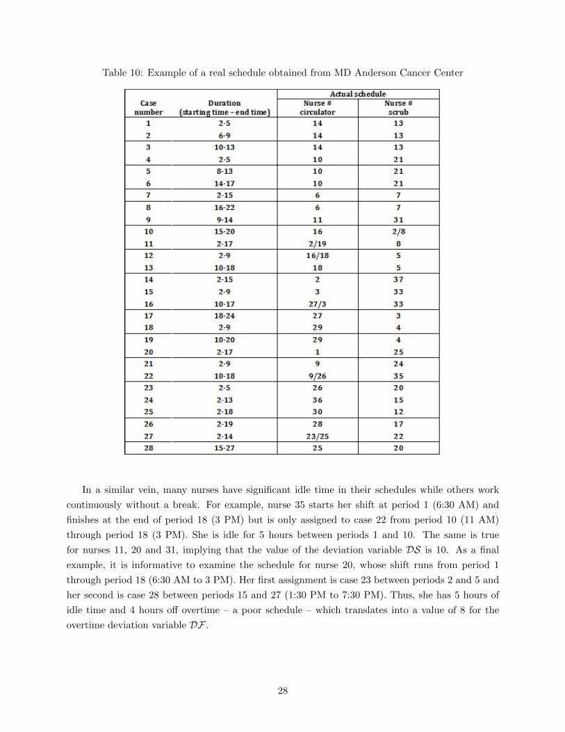
Table 10: Example of a real schedule obtained from MD Anderson Cancer Center
In a similar vein, many nurses have significant idle time in their schedules while others work
continuously without a break. For example, nurse 35 starts her shift at period 1 (6:30 AM) and
finishes at the end of period 18 (3 PM) but is only assigned to case 22 from period 10 (11 AM)
through period 18 (3 PM). She is idle for 5 hours between periods 1 and 10. The same is true
for nurses 11, 20 and 31, implying that the value of the deviation variable DS is 10. As a final
example, it is informative to examine the schedule for nurse 20, whose shift runs from period 1
through period 18 (6:30 AM to 3 PM). Her first assignment is case 23 between periods 2 and 5 and
her second is case 28 between periods 15 and 27 (1:30 PM to 7:30 PM). Thus, she has 5 hours of
idle time and 4 hours off overtime – a poor schedule – which translates into a value of 8 for the
overtime deviation variable DF .
28