DAC June 2003 1

Automatic Trace Analysisfor Logic of Constraints

Xi Chen, Harry HsiehUniversity of California, Riverside

Felice Balarin, Yosinori WatanabeCadence Berkeley Laboratories

DAC June 2003 2

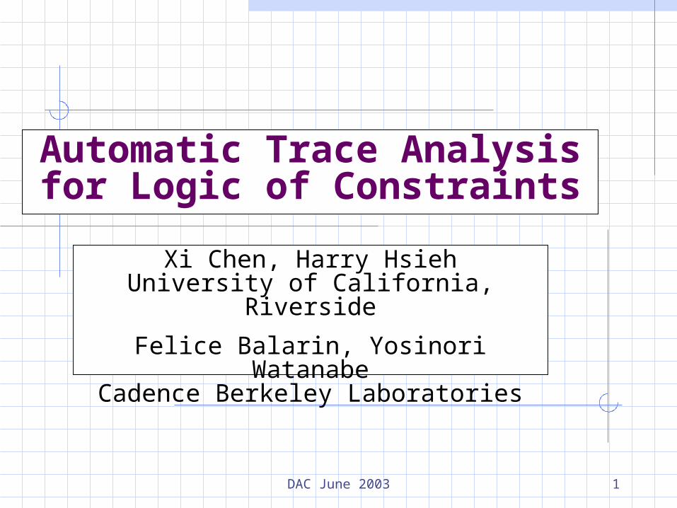
Outline

Introduction System-level design Logic of Constraints

Trace analysis methodology Methodology and algorithms Case studies

Proving LOC formulas

Summary

DAC June 2003 3

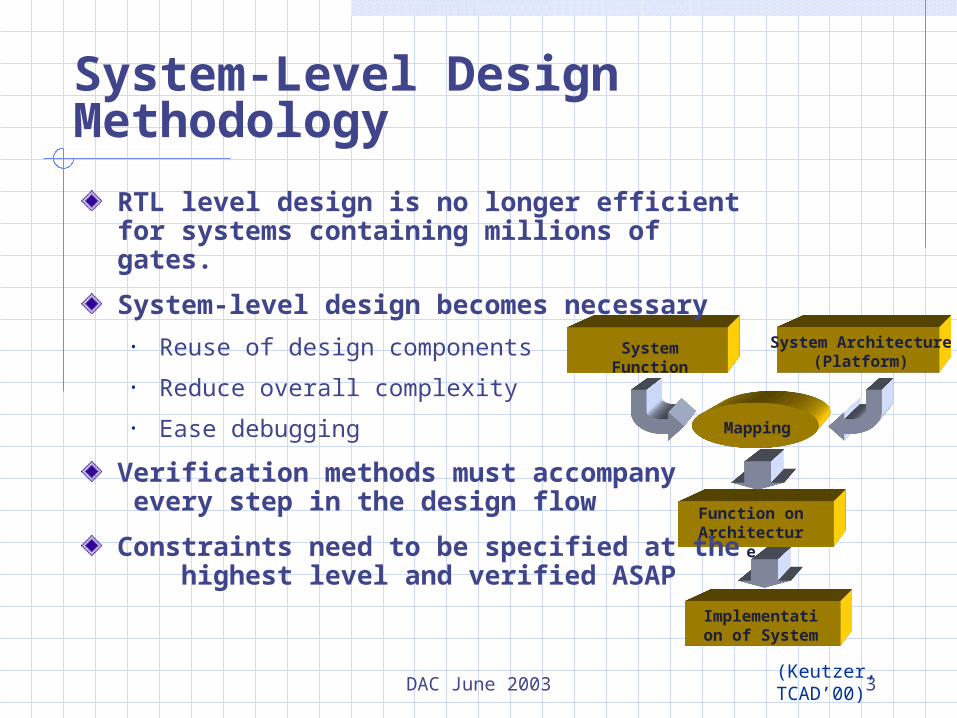
System-Level Design Methodology

System Architecture (Platform)

System Function

Mapping

Implementation of System

Function on Architecture

(Keutzer, TCAD’00)

RTL level design is no longer efficient for systems containing millions of gates.

System-level design becomes necessary• Reuse of design components

• Reduce overall complexity

• Ease debugging

Verification methods must accompany every step in the design flow

Constraints need to be specified at the highest level and verified ASAP

DAC June 2003 4

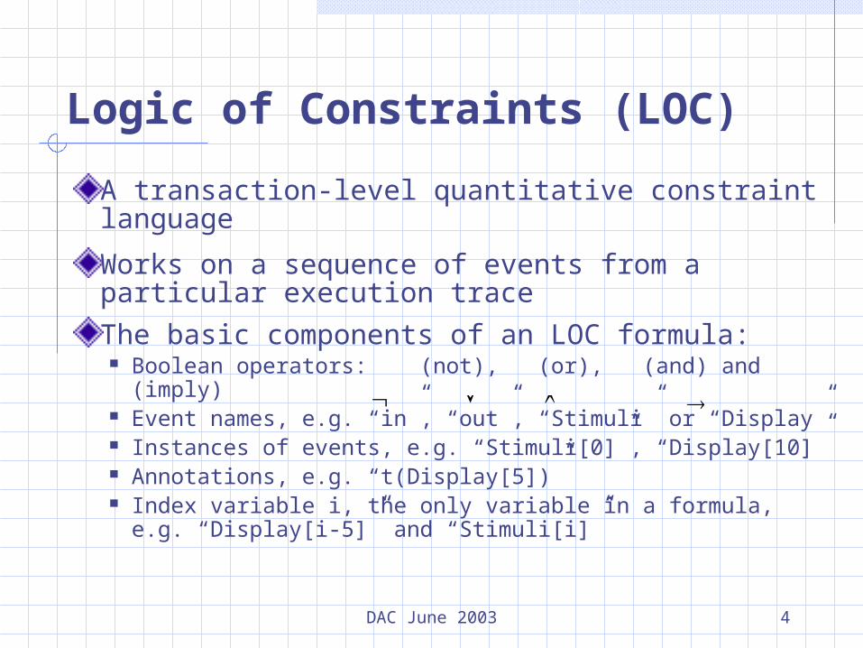
A transaction-level quantitative constraint language

Works on a sequence of events from a particular execution trace

The basic components of an LOC formula: Boolean operators: (not), (or), (and) and (imply) Event names, e.g. “in”, “out”, “Stimuli” or “Display” Instances of events, e.g. “Stimuli[0]”, “Display[10]” Annotations, e.g. “t(Display[5])” Index variable i, the only variable in a formula, e.g.

“Display[i-5]” and “Stimuli[i]”

Logic of Constraints (LOC)

DAC June 2003 5

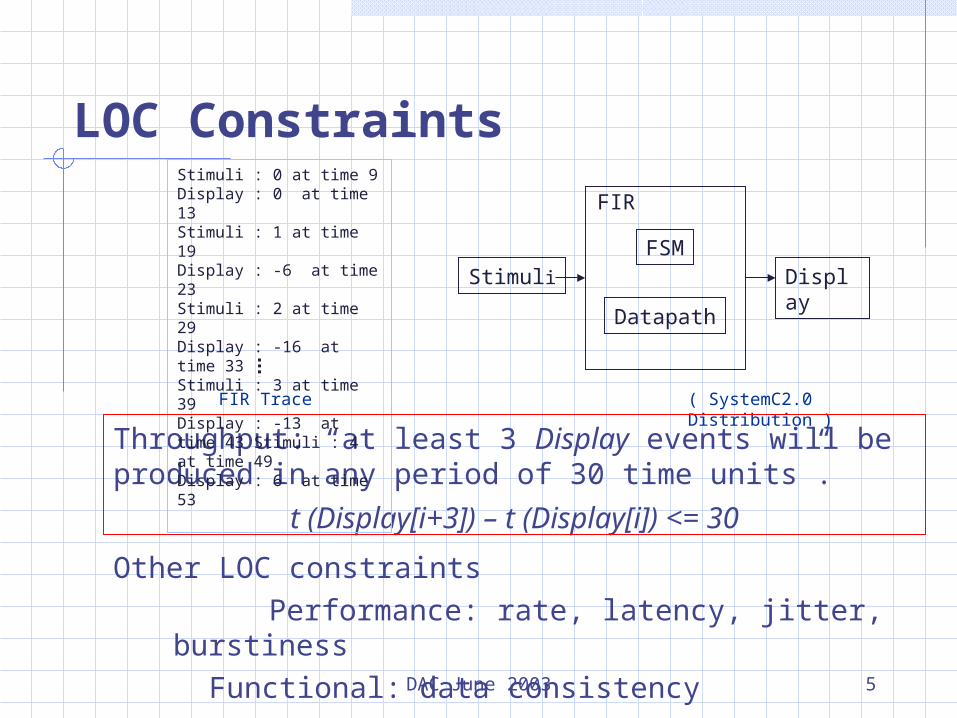
Throughput: “at least 3 Display events will be produced in any period of 30 time units”.

t (Display[i+3]) – t (Display[i]) <= 30

Other LOC constraints

Performance: rate, latency, jitter, burstiness

Functional: data consistency

StimuliFSM

Datapath

FIR

Display

( SystemC2.0 Distribution )

Stimuli : 0 at time 9Display : 0 at time 13Stimuli : 1 at time 19Display : -6 at time 23Stimuli : 2 at time 29Display : -16 at time 33Stimuli : 3 at time 39Display : -13 at time 43 Stimuli : 4 at time 49Display : 6 at time 53

FIR Trace

LOC Constraints

DAC June 2003 6

Assertion Languages(Related Work)

IBM’s Sugar and Synopsis' OpenVera

Good for both formal verification and simulation verification

Implemented as libraries to supportdifferent HDLs

Assertions are expressed with Boolean expressions, e.g. a[0:3] & b[0:3] =

“0000” Temporal logics, e.g. always !(a & b) HDL code blocks, e.g. handshake protocol

Mainly based on Linear Temporal Logic

DAC June 2003 7

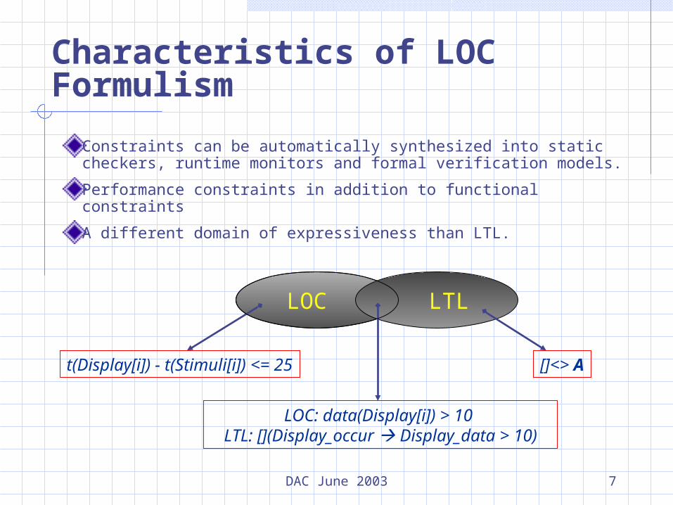
LOC LTL

t(Display[i]) - t(Stimuli[i]) <= 25

LOC: data(Display[i]) > 10 LTL: [](Display_occur Display_data > 10)

[]<> A

Characteristics of LOC Formulism

Constraints can be automatically synthesized into static checkers, runtime monitors and formal verification models.

Performance constraints in addition to functional constraints

A different domain of expressiveness than LTL.

DAC June 2003 8

Outline

Introduction

Trace analysis methodology Methodology and algorithms Case studies

Proving LOC formulas

Summary

DAC June 2003 9

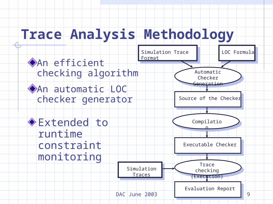
Trace Analysis Methodology

An efficient checking algorithm

An automatic LOC checker generator

Extended to runtime constraint monitoring

Simulation Trace Format LOC Formula

Automatic Checker Generation

Source of the Checker

Executable Checker

Compilation

Simulation Traces

Evaluation Report

Trace checking (Execution)

DAC June 2003 10End

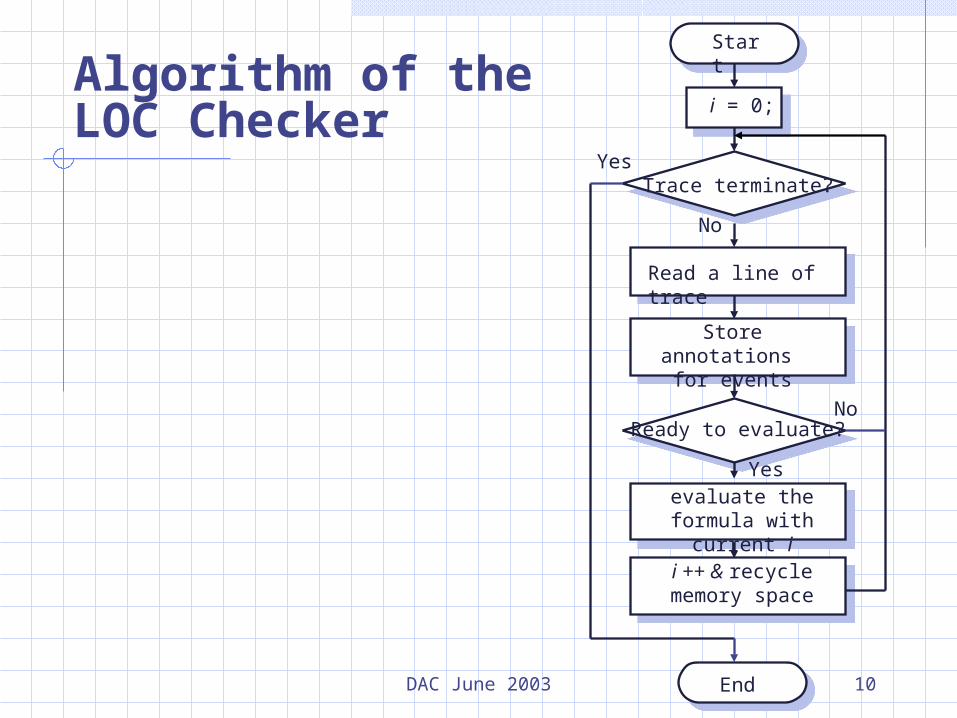
Start

i = 0;

Read a line of trace

Store annotations for events

evaluate the formula with current i

Trace terminate?

i ++ & recycle memory space

Ready to evaluate?

Yes

No

Yes

No

Algorithm of theLOC Checker

11

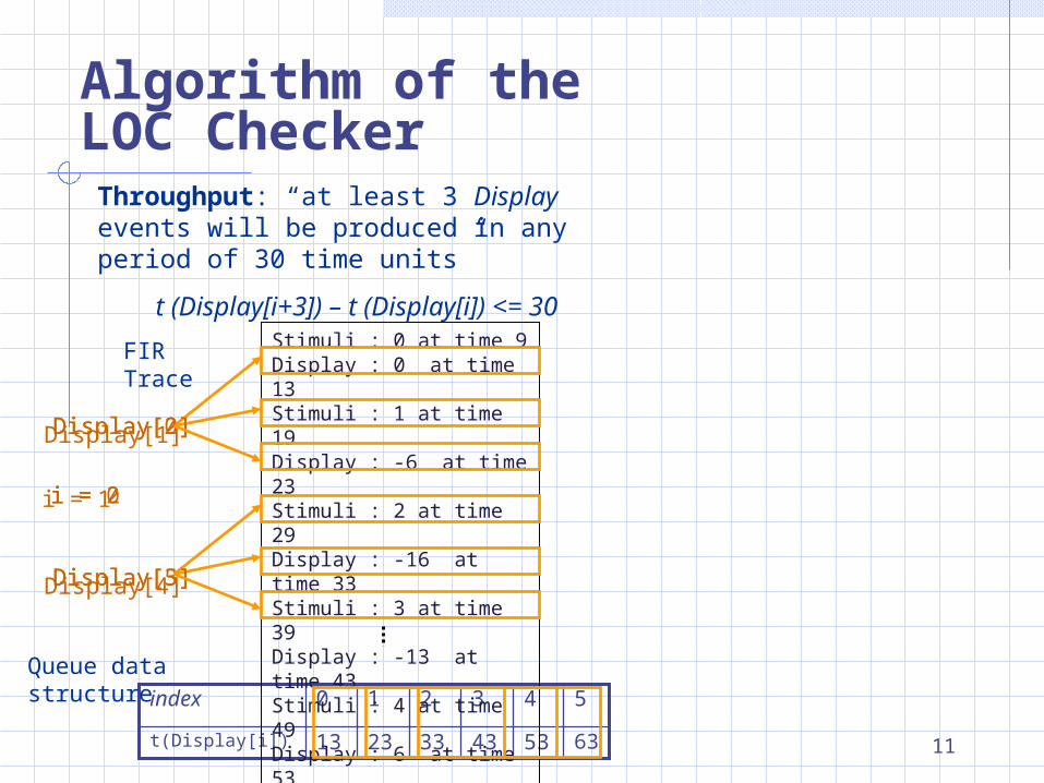
Throughput: “at least 3 Display events will be produced in any period of 30 time units”

t (Display[i+3]) – t (Display[i]) <= 30

FIR Trace

63

5

5343332313t(Display[i])

43210index

Queue data structure

Stimuli : 0 at time 9Display : 0 at time 13Stimuli : 1 at time 19Display : -6 at time 23Stimuli : 2 at time 29Display : -16 at time 33Stimuli : 3 at time 39Display : -13 at time 43Stimuli : 4 at time 49Display : 6 at time 53Stimuli : 4 at time 59Display : 6 at time 63

Algorithm of theLOC Checker

Display[0]

Display[3]

i = 0

Display[1]

Display[4]

i = 1

Display[2]

Display[5]

i = 2

DAC June 2003 12

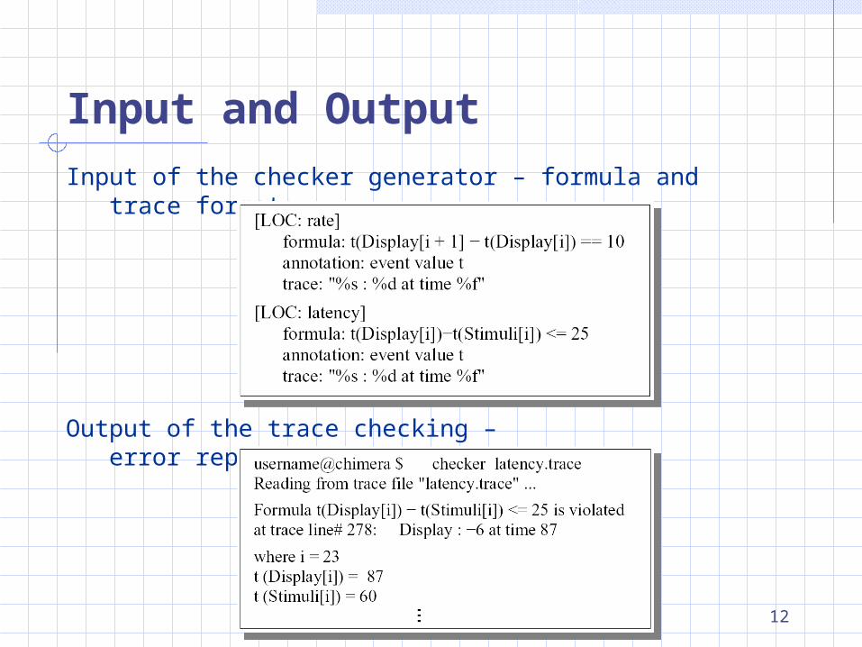
Input of the checker generator – formula and trace format:

Output of the trace checking – error report:

Input and Output

DAC June 2003 13

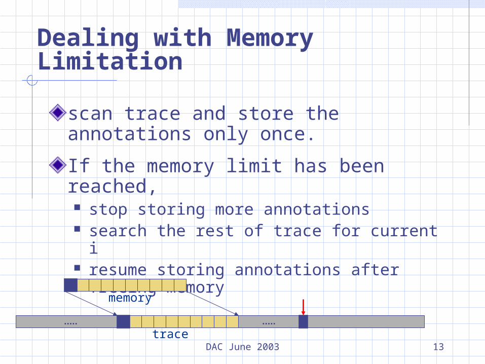
Dealing with Memory Limitation

scan trace and store the annotations only once.

If the memory limit has been reached, stop storing more annotations search the rest of trace for current i resume storing annotations after freeing

memory

memory

trace

DAC June 2003 14

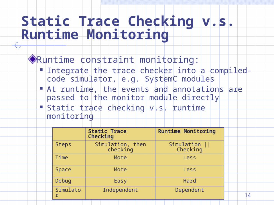
Static Trace Checking v.s. Runtime Monitoring

Runtime constraint monitoring: Integrate the trace checker into a compiled-

code simulator, e.g. SystemC modules At runtime, the events and annotations are

passed to the monitor module directly Static trace checking v.s. runtime monitoring

Static Trace Checking

Runtime Monitoring

Steps Simulation, then checking

Simulation || Checking

Time More Less

Space More Less

Debug Easy Hard

Simulator Independent Dependent

DAC June 2003 15

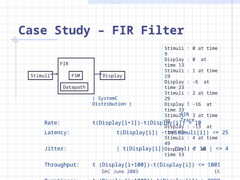
Rate: t(Display[i+1])-t(Display[i]) = 10

Latency: t(Display[i]) - t(Stimuli[i]) <= 25

Jitter: | t(Display[i]) - (i+1) * 10 | <= 4

Throughput: t (Display[i+100])-t(Display[i]) <= 1001

Burstiness: t (Display[i+1000])-t(Display[i]) > 9999

Stimuli FSM

Datapath

FIR

Display

( SystemC Distribution )

Stimuli : 0 at time 9Display : 0 at time 13Stimuli : 1 at time 19Display : -6 at time 23Stimuli : 2 at time 29Display : -16 at time 33Stimuli : 3 at time 39Display : -13 at time 43Stimuli : 4 at time 49Display : 6 at time 53

FIR Trace

Case Study – FIR Filter

DAC June 2003 16

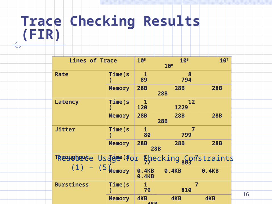
Lines of Trace 105 106 107 108

Rate Time(s) 1 8 89 794

Memory 28B 28B 28B 28B

Latency Time(s) 1 12 120 1229

Memory 28B 28B 28B 28B

Jitter Time(s) 1 7 80 799

Memory 28B 28B 28B 28B

Throughput Time(s) 1 7 77 803

Memory 0.4KB 0.4KB 0.4KB 0.4KB

Burstiness Time(s) 1 7 79 810

Memory 4KB 4KB 4KB 4KB

Resource Usage for Checking Constraints (1) – (5)

Trace Checking Results (FIR)

DAC June 2003 17

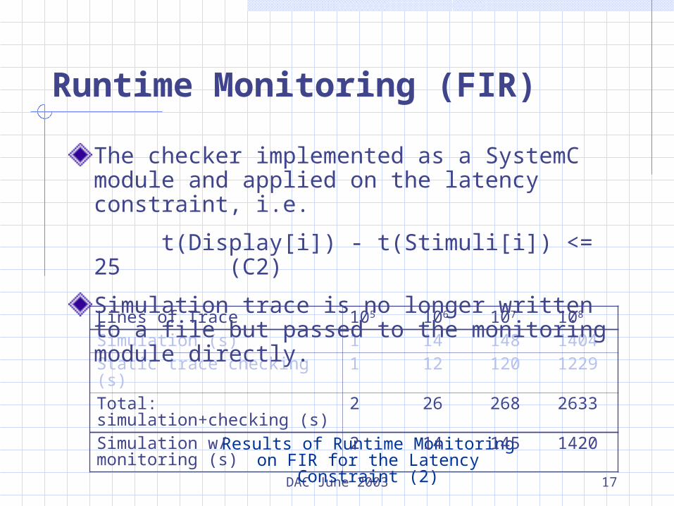
Results of Runtime Monitoring on FIR for the Latency Constraint (2)

Lines of Trace 105 106 107 108

Simulation (s) 1 14 148 1404Static trace checking (s) 1 12 120 1229Total: simulation+checking (s) 2 26 268 2633Simulation w/ monitoring (s) 2 14 145 1420

Runtime Monitoring (FIR)

The checker implemented as a SystemC module and applied on the latency constraint, i.e.

t(Display[i]) - t(Stimuli[i]) <= 25(C2)

Simulation trace is no longer written to a file but passed to the monitoring module directly.

DAC June 2003 18PIP trace

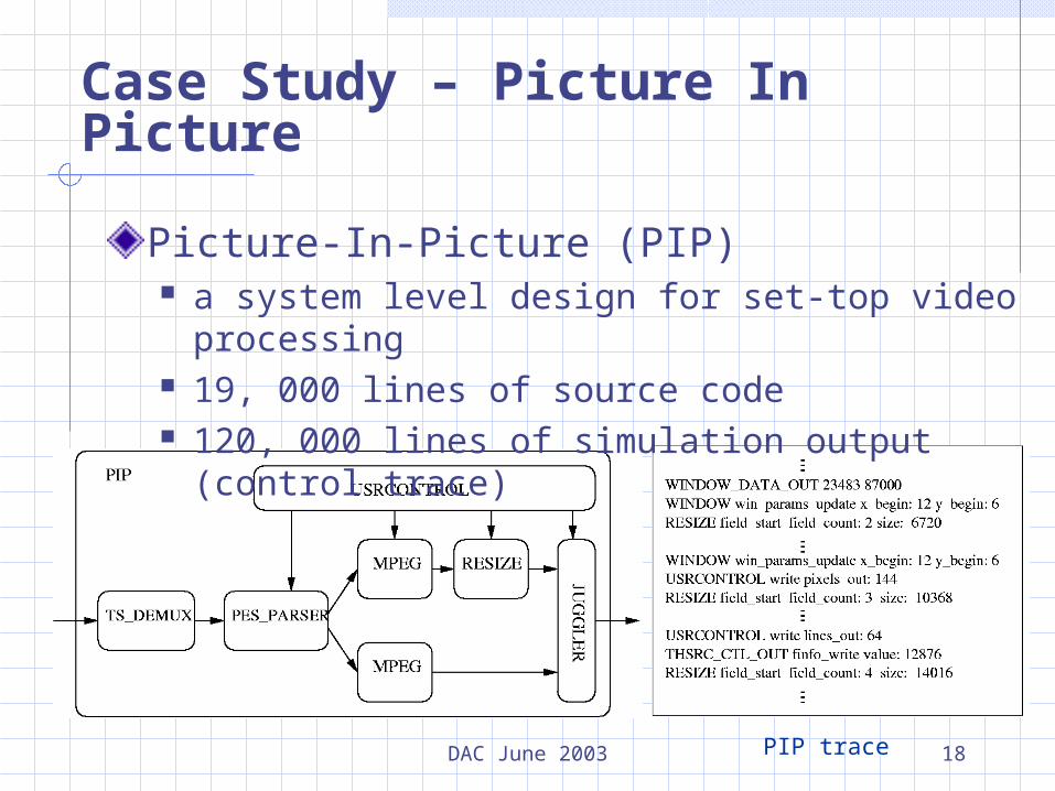
Case Study – Picture In Picture

Picture-In-Picture (PIP) a system level design for set-top video

processing 19, 000 lines of source code 120, 000 lines of simulation output (control

trace)

DAC June 2003 19

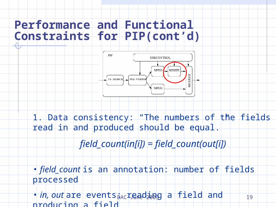
1. Data consistency: “The numbers of the fields read in and produced should be equal.”

field_count(in[i]) = field_count(out[i])

• field_count is an annotation: number of fields processed

• in, out are events: reading a field and producing a field

Performance and Functional Constraints for PIP(cont’d)

DAC June 2003 20

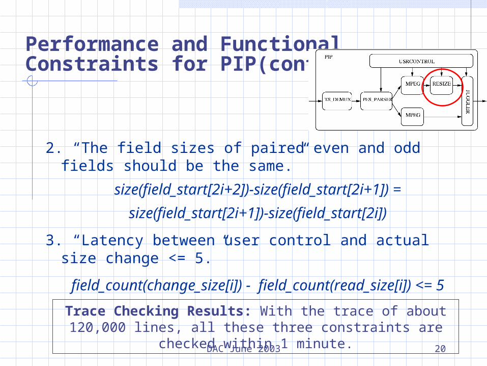
2. “The field sizes of paired even and odd fields should be the same.”

size(field_start[2i+2])-size(field_start[2i+1]) =

size(field_start[2i+1])-size(field_start[2i])

3. “Latency between user control and actual size change <= 5.”

field_count(change_size[i]) - field_count(read_size[i]) <= 5

Trace Checking Results: With the trace of about 120,000 lines, all these three constraints are checked within 1 minute.

Performance and Functional Constraints for PIP(cont’d)

DAC June 2003 21

Outline

Introduction

Trace analysis methodology

Proving LOC formulas

Summary

DAC June 2003 22

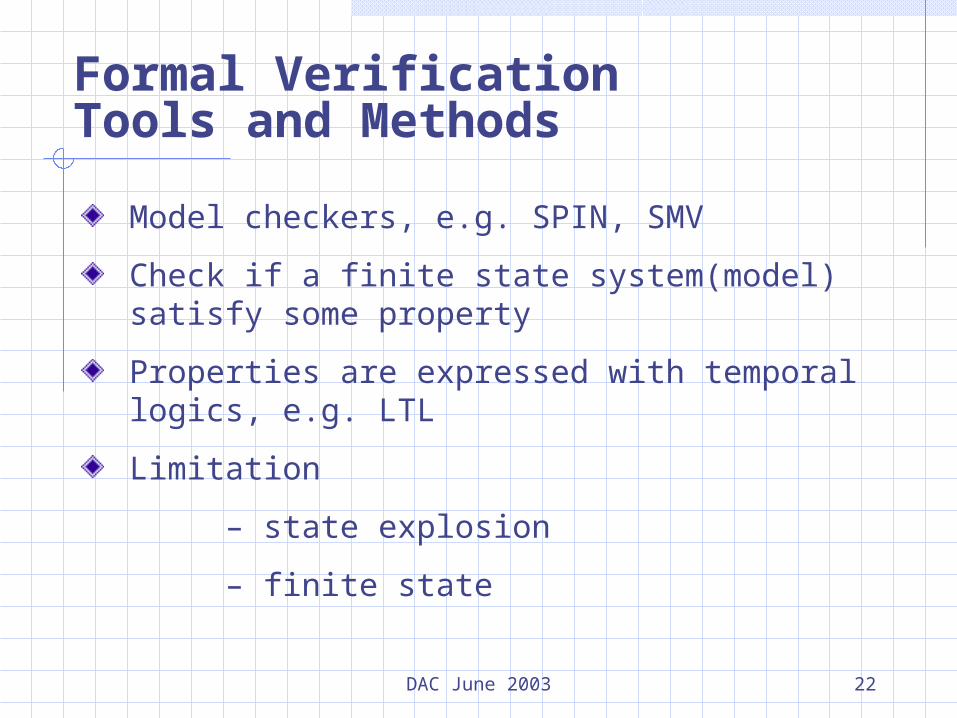
Formal Verification Tools and Methods

Model checkers, e.g. SPIN, SMV

Check if a finite state system(model) satisfy some property

Properties are expressed with temporal logics, e.g. LTL

Limitation

– state explosion

– finite state

DAC June 2003 23

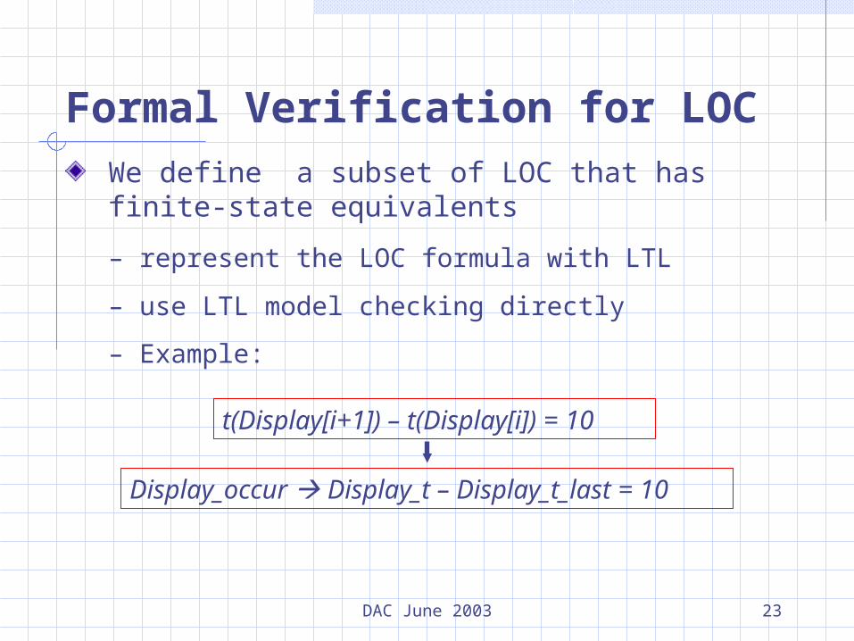
Formal Verification for LOCWe define a subset of LOC that has finite-state equivalents

– represent the LOC formula with LTL

– use LTL model checking directly

– Example:

t(Display[i+1]) – t(Display[i]) = 10

Display_occur Display_t – Display_t_last = 10

DAC June 2003 24

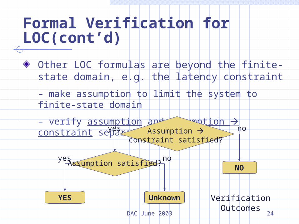
Formal Verification for LOC(cont’d)

Other LOC formulas are beyond the finite-state domain, e.g. the latency constraint

– make assumption to limit the system to finite-state domain

– verify assumption and assumption constraint separately Assumption constraint

satisfied?

Assumption satisfied?

YES

NO

Unknown

yes

yes

no

no

Verification Outcomes

DAC June 2003 25

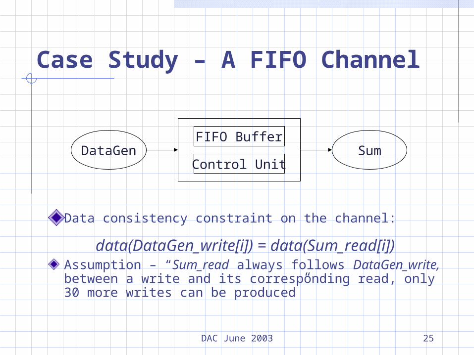
Data consistency constraint on the channel:

Assumption – “Sum_read always follows DataGen_write, between a write and its corresponding read, only 30 more writes can be produced”

data(DataGen_write[i]) = data(Sum_read[i])

Case Study – A FIFO Channel

DataGen SumFIFO Buffer

Control Unit

DAC June 2003 26

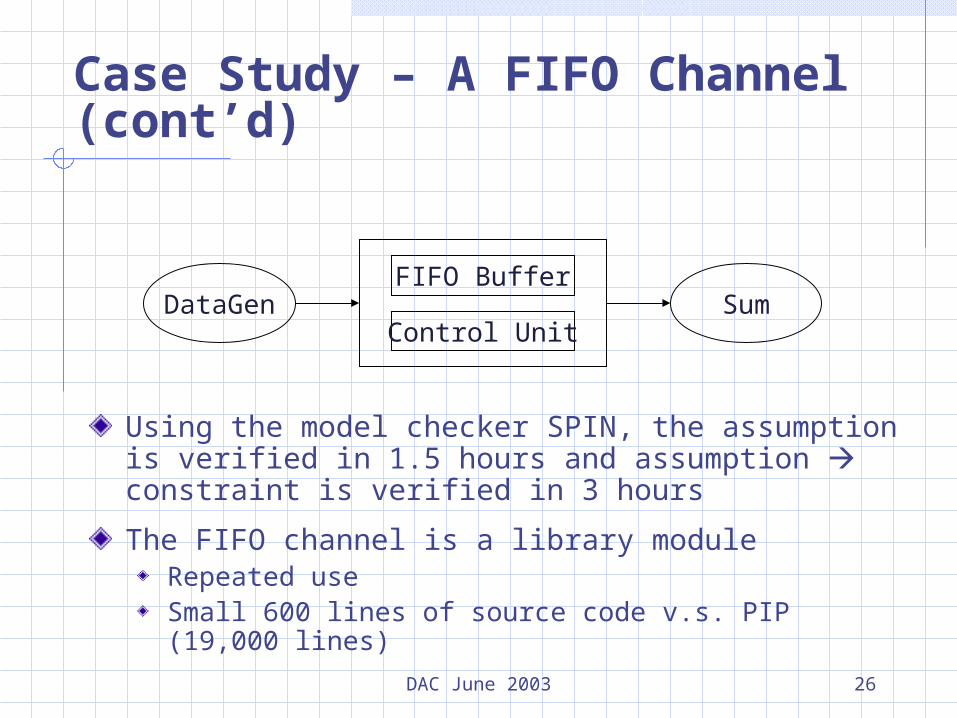
Using the model checker SPIN, the assumption is verified in 1.5 hours and assumption constraint is verified in 3 hours

The FIFO channel is a library module Repeated useSmall 600 lines of source code v.s. PIP (19,000 lines)

Case Study – A FIFO Channel (cont’d)

DataGen SumFIFO Buffer

Control Unit

DAC June 2003 27

Summary

LOC is useful and is different from LTL

Automatic trace analysis

Case studies with large designs and traces

Formal verification approach

DAC June 2003 28

Thank You!