Embed Size (px)
Citation preview
H2020 5G-TRANSFORMER Project
Grant No. 761536
Experimentation results and evaluation of achievements in
terms of KPIs
Abstract
This deliverable first summarizes the relationship between the performance KPIs
defined by 5G-PPP and the KPIs considered in the 5G-TRANSFORMER project. Then,
it shows by means of Proofs of Concept and additional experiments and simulations,
how the 5G-TRANSFORMER project contributes towards reaching the targeted 5G-
PPP KPI objectives.
Experimentation results and evaluation of achievements in terms of KPIs 2
H2020-761536
Document properties
Document number D5.3
Document title Experimentation results and evaluation of achievements in terms of KPIs
Document responsible Farouk Messaoudi (BCOM)
Document editor Farouk Messaoudi (BCOM)
Editorial team Luca Valcarenghi (SSSA), Farouk Messaoudi (BCOM)
Target dissemination level Public
Status of the document Final
Version 1.0
Production properties
Reviewers Andres Garcia-Saavedra (NECLE), Charles Turyagyenda (IDCC), Francesco D’Andria (ATOS), Carlos J. Bernardos (UC3M)
Disclaimer
This document has been produced in the context of the 5G-TRANSFORMER Project.
The research leading to these results has received funding from the European
Community's H2020 Programme under grant agreement Nº H2020-761536.
All information in this document is provided “as is" and no guarantee or warranty is
given that the information is fit for any particular purpose. The user thereof uses the
information at its sole risk and liability.
For the avoidance of all doubts, the European Commission has no liability in respect of
this document, which is merely representing the authors view.
Experimentation results and evaluation of achievements in terms of KPIs 3
H2020-761536
Table of Contents List of Contributors ........................................................................................................ 5
List of Figures ............................................................................................................... 6
List of Tables ................................................................................................................ 8
List of Acronyms ........................................................................................................... 9
Executive Summary and Key Contributions ................................................................ 11
1 Introduction .......................................................................................................... 12
2 KPIs Overview ..................................................................................................... 13
2.1 5G-PPP Performance KPIs ........................................................................... 13
2.2 5G-TRANSFORMER KPIs ............................................................................ 13
2.3 Mapping of 5G-TRANSFORMER KPIs to 5G-PPP KPIs ............................... 16
3 Selected Proofs of Concept ................................................................................. 18
3.1 Automotive ................................................................................................... 18
3.2 Entertainment ............................................................................................... 19
3.3 E-Health ....................................................................................................... 20
3.4 E-Industry ..................................................................................................... 21
3.5 MNO/MVNO ................................................................................................. 22
3.6 Contribution of PoCs to 5G-PPP Performance KPIs ..................................... 24
4 Experiments, Measurements, Results .................................................................. 26
4.1 Automotive ................................................................................................... 26
4.1.1 Considered KPI(s) and benchmark ........................................................ 26
4.1.2 Experiment Scenario and Measurement Methodology ........................... 27
4.1.3 Results .................................................................................................. 30
4.2 Entertainment ............................................................................................... 34
4.2.1 Considered KPI(s) and benchmark ........................................................ 34
4.2.2 Experiment Scenario and Measurement Methodology ........................... 34
4.2.3 Results .................................................................................................. 36
4.3 E-Health ....................................................................................................... 38
4.3.1 Considered KPI(s) and benchmark ........................................................ 38
4.3.2 Experiment Scenario and Measurement Methodology ........................... 39
4.3.3 Results .................................................................................................. 40
4.4 E-Industry ..................................................................................................... 46
4.4.1 Considered KPI(s) and benchmark ........................................................ 46
4.4.2 Experiment Scenario and Measurement Methodology ........................... 46
4.4.3 Results .................................................................................................. 48
4.5 MNO/MVNO ................................................................................................. 50
Experimentation results and evaluation of achievements in terms of KPIs 4
H2020-761536
4.5.1 Considered KPI(s) and benchmark ........................................................ 50
4.5.2 Experiment Scenario and Measurement Methodology ........................... 50
4.5.3 Results .................................................................................................. 51
5 Additional evaluation ............................................................................................ 56
5.1 Real-time computation in virtualized environments ....................................... 56
5.1.1 Considered KPI(s) and benchmark ........................................................ 56
5.1.2 Experiment/Simulation Scenario and Measurement Methodology ......... 57
5.1.3 Results .................................................................................................. 58
5.1.4 Conclusions ........................................................................................... 61
5.2 Experimental Demonstration of a 5G Network Slice Deployment through the
5G-TRANSFORMER Architecture ........................................................................... 62
5.2.1 Considered KPI(s) and benchmark ........................................................ 62
5.2.2 Experiment/Simulation Scenario and Measurement Methodology ......... 62
5.2.3 Results .................................................................................................. 64
5.3 Additional evaluation on MTP-related KPIs ................................................... 65
5.3.1 5GT-MTP algorithms contributing to KPIs .............................................. 65
5.3.2 Results and impacted KPIs .................................................................... 69
5.3.3 Summary table ...................................................................................... 77
6 Summary ............................................................................................................. 81
7 References .......................................................................................................... 82
8 Appendix A .......................................................................................................... 85
Experimentation results and evaluation of achievements in terms of KPIs 5
H2020-761536
List of Contributors Partner Short Name Contributors
UC3M Kiril Antevski, Borja Nogales, Winnie Nakimuli, Carlos J. Bernardos
TEI Teresa Pepe, Paola Iovanna, Erin Seder
ATOS Arturo Zurita, Jose Enrique Gonzalez, Francesco D’Andria
BCOM Farouk Messaoudi, Cao-Thanh Phan
NXW Giada Landi
CRF Aleksandra Stojanovic, Marina Giordanino
CTTC Ricardo Martínez, Luca Vettori, Jordi Baranda, Josep Mangues, Engin Zeydan, Manuel Requena, Ramon Casellas
POLITO Carla Fabiana Chiasserini, Giuseppe Avino SSSA Luca Valcarenghi, Koteswararao Kondepu
NOK-N Thomas Deiß, Dieter Knüppel
NEC Andres Garcia-Saavedra, Josep Xavier Salvat
Experimentation results and evaluation of achievements in terms of KPIs 6
H2020-761536
List of Figures Figure 1: Evs workflow ................................................................................................ 18
Figure 2: Design of OLE and UHD use cases ............................................................. 20
Figure 3: (A) Monitoring of patients (b) emergency case ............................................. 21
Figure 4: Schematic of the EIndustry cloud robotics demonstrator .............................. 22
Figure 5: Wireless Edge Factory (EPC) ...................................................................... 24
Figure 6: PSR results .................................................................................................. 30
Figure 7: Cdf of the processing time of the evs application .......................................... 32
Figure 8: Cdf of the end-to-end latency as a function of the vehicle density ................ 32
Figure 9: Percentage of collisions detected, detected in time and false-negatives ...... 33
Figure 10: Percentage of false-positives over the denm received................................ 33
Figure 11: Distances between cars involved in false positive detections ..................... 34
Figure 12: Demo scenario of the entertainment use case in 5tonic testbed ................. 35
Figure 13: Round Trip Time between the Origin server and the Cache server............. 36
Figure 14: User data rate obtained from the metrics of the video player ...................... 36
Figure 15: vCDN service creation time including Origin server, Cache server and
Webserver .................................................................................................................. 37
Figure 16: Scale-out time of a Cache server in the vCDN service ............................... 38
Figure 17: Latency CDF from UE to central eserver .................................................... 41
Figure 18: Latency CDF from UE to local eserver ....................................................... 42
Figure 19: Total bandwidth between an ue and local eserver ...................................... 45
Figure 20: Jitter between an ue and local eserver ....................................................... 45
Figure 21: Eindustry cloud robotics network scheme................................................... 47
Figure 22: Round trip-time (rtt) latency, the time in seconds of the path from the core
network to the service robots and back, poc 4.1(left) and poc 4.2(right) ...................... 48
Figure 23: KPI ser for poc id 4.2 taken at the mtp level ............................................... 50
Figure 24: Cdf of service creation time (ser) for mvno use case considering the urllc
service obtained by increasing the flavour of the mme ................................................ 52
Figure 25: Service creation time (ser) for mvno use case considering the urllc service
versus increasing the flavour of the mme. the box plot includes the 10th, 25th, median,
75th, and 90th percentiles of these times. ................................................................... 53
Figure 26: Infrastructure cost per month generated from the MVNO use case
considering the URLLC service type (composed of 10 VNFs) deployed on three
datacenter types, considereing several flavours for the MME ...................................... 54
Figure 27: Infrastructure cost per month generated from the mvno use case considering
the urllc service typedeployed on three datacenter types, considereing scale-in for the
mme ........................................................................................................................... 55
Figure 28: Proprietary measurement for optimized Linux ............................................ 60
Figure 29: Cyclictest measurements for optimized Linux ............................................. 60
Figure 30: Proprietary measurements for non-optimized Linux ................................... 61
Figure 31: 5G Network slice deployment demo Setup ................................................. 63
Figure 32: Demo workflow .......................................................................................... 64
Figure 33: Representation of the network service ....................................................... 64
Figure 34: Mobile screen capture ................................................................................ 65
Figure 35: Considered 5GT-SO / 5GT-MTP controlled DC and WAN (Packet over Flexi-
Grid Optical) Scenario ................................................................................................. 67
Figure 36: VM adaptation algorithm ............................................................................ 69
Figure 37: Power consumption yielded by the heuristic algorithm vs. the optimum...... 71
Experimentation results and evaluation of achievements in terms of KPIs 7
H2020-761536
Figure 38: Number of servers used by the heuristic algorithm vs. the optimum ........... 71
Figure 39: Unused vCPUs left by the heuristic algorithm vs. the optimum ................... 71
Figure 40: Ratio of RAN centralized functions in swiss, romanian and italian topologies
for different values of CU capacity and traffic load. ..................................................... 74
Figure 41: Number of Benders iterations in Swiss, Romanian and Italian .................... 75
Figure 42: RAN centralization (top) and system cost (bottom) for Italian topology (R3)
for 𝛼𝑛 = 𝛼0 = 1 and variable transport costs, for C-RAN, D-RAN and FluidRAN
architectures. .............................................................................................................. 76
Figure 43: RAN centralization (top) and cost (bottom) for different MEC process
characteristics and loads. Non-MEC load is 10 Mb/s for all RUs ................................. 77
Experimentation results and evaluation of achievements in terms of KPIs 8
H2020-761536
List of Tables Table 1: 5G-PPP Performance KPIs with their relevance ............................................ 13
Table 2: KPIs considered in 5G-TRANSFORMER ...................................................... 14
Table 3: Mapping of 5G-TRANSFORMER KPIs to 5G-PPP performance KPIs ........... 17
Table 4: Contributions to the 5G-PPP performnce KPIs by the considered PoCs ........ 25
Table 5: KPIs considered in the Automotive PoC ........................................................ 27
Table 6: Different latency measurement methodologies for different PoC releases ..... 27
Table 7: Different Reliability measurement methodologies for diffeerent PoC releases28
Table 8: Different density measurement methodologies for different PoC releases ..... 29
Table 9: Entertainment use case considered KPIs ...................................................... 34
Table 10: Latency measurement methodology for the different PoCs.......................... 35
Table 11 User data rate measurement methodology for the different PoCs ................. 35
Table 12 Service creation time measurement methodology ........................................ 36
Table 13: E-Health Mapping: PoCs and high-level KPIs .............................................. 39
Table 14: Central eserver latency ............................................................................... 41
Table 15: Local eServer latency .................................................................................. 41
Table 16: Emergency interventions in a year (May 2018 - April 2019) ......................... 43
Table 17: Reliability KPI measurements ...................................................................... 43
Table 18: Accuracy measures used to measure positioning of mobile devices ............ 44
Table 19: Accuracy measurements of different mobile devices ................................... 44
Table 20: Total bandwidth ........................................................................................... 44
Table 21: Jitter ............................................................................................................ 45
Table 22: KPI mapping to current performance specifications and future targets ........ 46
Table 23: Latency measurement methodologies for EIndustry PoC releases .............. 47
Table 24: Reliability measurement methodologies for eindustry poc releases ............. 48
Table 25: Service creation time measurement methodologies for eindustry poc releases
................................................................................................................................... 48
Table 26: MVNO considered KPIs .............................................................................. 50
Table 27: Optimized Linux configuration boot parameters ........................................... 57
Table 28: Optimized Linux configuration dynamic settings .......................................... 58
Table 29: Typical distribution of measured values ....................................................... 59
Table 30: Topologies used in evaluation of FluidRAN ................................................. 72
Table 31: MTP KPIs evaluation – summary table ......................................................... 78
Table 32: Hardware Details ......................................................................................... 85
Experimentation results and evaluation of achievements in terms of KPIs 9
H2020-761536
List of Acronyms Acronym Description
5G-PPP 5G Public Private Partnership
5GT 5G-TRANSFORMER Project RTT Round Trip Time
5G-T CI 5G-TRANSFORMER Continuous Integration platform
5GT-MTP 5G-TRANSFORMER Mobile Transport and Computing Platform
5GT-SO 5G-TRANSFORMER Service Orchestrator
5GT-VS 5G-TRANSFORMER Vertical Slicer
AGV Automated Guided Vehicle
AP Action Point
A-COV Availability (related to coverage)
A-RES Availability (related to resilience)
CAGR Compound Annual Growth Rate
CAM Cooperative Awareness Messages
CAPEX Capital Expenditure CDF Cumulative Distribution Function
CI Continuous Integration
CIM Cooperative Information Manager
C-ITS Cooperative Intelligent Transport Systems
CON Confidentiality
COTS Commercial of the Shelf
CP/UP Control Plane / User Plane
CR Cloud Robotics
CST Cost
CTO Chief Technology Officer
CUPS Control / User Plane Separation
D2D Device-to-Device (communication) DC Data Center
DEN Device density
DENM Decentralized Environmental Notification Message
DoA Description of Action
E2E End to End
EPC Evolved Packet Core
EVS Extended Virtual Sensing
HSS Home Subscriber Server
HW Hardware
ICA Intersection Collision Avoidance
ICT Information and communication technology
INF Infrastructure
INT Integrity KPI Key Performance Indicator
LAT End-to-end (E2E) latency
LTE Long-Term Evolution
MANO Management and Orchestration
MCPTT Mission Critical Push to Talk
MEC Multi-access Edge Computing
MME Mobility Management Entity
MNO/MVNO Mobile Network Operator / Mobile Virtual Network Operator
MOB Mobility
MPEG Moving Picture Experts Group
Experimentation results and evaluation of achievements in terms of KPIs 10
H2020-761536
NBI North-Bound Interface
NFV Network Function Virtualization
NFVI-PoP Network Function Virtualization Point of Presence
NFV-NS Network Service
NFVO NFV Orchestrator
NRG Energy reduction NSD Network Service Descriptor
OPEX Operational Expenditure
OTT Over The Top media services
PNF Physical Network Function
PoC Proof-of-Concept
POS Positioning accuracy
QoE Quality of Experience
RAN Radio Access Network
RANG Communication Range
REL Reliability
RTT Round Trip Time
RSU Road Side Unit SER Service creation time
SGi Service Gateway interface
SLA Service Level Agreement
SW Software
TRA Traffic type
UC Use Case
UDR User data rate
UE User Equipment
UHD Ultra-High Definition
vCDN virtual Content Distribution Network
vEPC virtual EPC
VA Virtual Application VDU Virtual Deployment Unit
VNF Virtualized Network Function
VNFM Virtual Network Functions Manager
VPN Virtual Private Network
VSD Vertical Service Descriptor
VxLAN Virtual eXtensible Local Area Network
WAN Wide Area Network
WIM WAN Infrastructure Manager
WP1 5GT Work Package 1
WP2 5GT Work Package 2
WP3 5GT Work Package 3
WP4 5GT Work Package 4 WP5 5GT Work Package 5
Experimentation results and evaluation of achievements in terms of KPIs 11
H2020-761536
Executive Summary and Key Contributions This deliverable addresses one of the main goals of the 5G-TRANSFORMER project:
demonstrating and validating the technology components designed and developed in
the project. This is done in WP5 – in charge of integrating all components provided by
WP2, WP3 and WP4 – by conducting different proofs of concept (PoCs) to validate the
5G-TRANSFORMER architecture.
The PoCs are used to evaluate whether the solutions developed for the 5G-
TRANSFORMER framework achieve the Key Performance Indicators (KPI) expected
by the considered verticals. These solutions are compared to the state of the art or the
used ones in common practice to evaluate the performance gain achieved in terms of
KPIs. The results are extracted from the experiments’ realization, focusing on
quantitative and qualitative KPIs defined in 5G Public Private Partnership (5G-PPP)
such as mobility, latency, energy efficiency, and service creation time.
This deliverable provides definitions for the considered 5G-TRANSFORMER KPIs and
how they are measured, as well as their mapping to the G-PPP performance KPIs.
Moreover, it presents an initial evaluation of the 5G-TRANSFORMER KPIs conducted
in WP5. The evaluation is performed through POCs demonstrated in the 5G-
TRANSFORMER testbed and via simulations. The PoCs considered in the
performance evaluation are: Extended Virtual Sensing (EVS) for Automotive, On-site
Live Experience (OLE) and Ultra High-Definition (UHD) for Entertainment, a heart-
attack emergency use case for E-Health, cloud robotics for E-Industry, and 4G/5G
Network as a Service (NaaS) for MNO/MVNO. In addition to evaluation by the PoCs,
additional measurements have been performed on individual components and are
reported in this deliverable. The initial evaluation will be extended after the next stage
of the software component integration, which will allow comprehensive testing of the
final 5G-TRANSFORMER platform.
The key contributions and the associated outcomes of this deliverable are the following:
• The description of the KPIs and the mapping between the 5G-PPP and the 5G-
TRANSFORMER KPIs.
• The final list of the demonstrations and PoCs that were conducted, as well as
their implementation and development roadmap. This roadmap has been
aligned with the implementation steps of the correspondent work packages,
providing the 5G-TRANSFORMER platform components used to deploy the use
cases.
• PoCs planning per use case, their description and demonstrated KPIs, including
the initial performance results.
• Additional KPI evaluations provided through demos.
• Contribution of additionally developed algorithms to the KPIs.
• Verifying that the 5G-TRANSFORMER platform components are ready to be
fully integrated and start of the final field trials. Indeed, via the different POCs
we could demonstrate the the functionality of these components, which are
ready to deliver and integrate together.
Experimentation results and evaluation of achievements in terms of KPIs 12
H2020-761536
1 Introduction This deliverable validates and evaluates the 5G-TRANSFORMER technology
components that have been designed in the 5G-TRANSFORMER Work Packages 1, 2,
3, and 4 (WP1, WP2, WP3 and WP4, respectively) through simulations as well as
experimentations in an end-to-end testbed.
5G-TRANSFORMER provides an innovative approach to build 5G services while
improving over existing solutions. Its goals include:
• Handling service requests with stringent service criteria such as ultra low
latency communication service,
• Fast vertical service provisioning and delivery,
• Maintaining and improving the service performance to meet a specific level or
user experience,
• Maximizing service offers in terms of connected devices and traffic densities in
an environment where resources can be fluctuating and limited or even scarce,
• Reducing the expenditure and resource consumption as well as increasing the
service assurance.
To achieve these objectives, the project relies on a modular and hierarchical
architecture comprising 3 layers (5GT-VS, 5GT-SO and 5GT-MTP) with abstract
interfaces to isolate the components. This architecture is based on the concept of
network slicing using ETSI NFV network services to describe them. The 5G-
TRANSFORMER components include algorithms:
• To translate high level service criteria into requirements for the low level
infrastructure provider,
• To perform multi-objective optimization of compute and network resource
selection and allocation, and
• To validate the conformity of service performance to service level agreements
(SLA) based on data collected from the monitoring and to automatically
remediate by appropriate actions.
The KPIs are metrics used to reflect progress toward the goals defined for the project.
They also highlight the vertical service requirements of the use cases (UC) and steered
the realization of the proofs of concept. The UCs provided by the different verticals are
implemented and used as a field of experimentation and simulation to measure the
performance, analyse the results and evaluate the benefits of the 5G-TRANSFORMER
system. Through the POCs, the feasibility of the 5G-TRANSFORMER system for
managing vertical services is demonstrated. The POCs and the software simulations
contribute to the measurement of the KPIs to validate the objectives of the project.
The deliverable is organized as follows: Section 2 presents an overview of the 5G-PPP
contractual KPIs and the KPIs described in 5G-TRANSFORMER, as well as a mapping
between them. In Section 3, the demonstrated PoCs are described. Section 4 focuses
on the experiments, measurements, and results obtained from PoCs. Additional
evaluation is provided in Section 5, which presents KPI evaluation for real-time
computation in virtualized environments, experimental demonstrations of the 5G
network slice deployment using the 5G-TRANSFORMER architecture, as well as
describing the contribution of several additional algorithms to the 5G-TRANSFORMER
KPIs.
Experimentation results and evaluation of achievements in terms of KPIs 13
H2020-761536
2 KPIs Overview This section provides an overview of the KPIs considered by 5G-TRANSFORMER and
their relationship with the 5G-Public Private Partnership (5G-PPP) contractual KPIs.
The consolidation of the KPIs is already reported in D5.2 [1].
2.1 5G-PPP Performance KPIs
Table 1 reports the 5G-PPP Performance KPIs as already reported in D1.1 [2] and
specified in [3], their definition, and the relevance for the 5G-TRANSFORMER project
(Note: the KPIs “Enabling advanced user controlled privacy” are very important but they
are already the focus of other projects in 5G-PPP. Thus, it is not targeted by the 5G-
TRANSFORMER project). As summarized in Table 1, the project is mainly focusing on
P1, P2, and P3 while P4 and P5 are perceived of lower relevance. This is motivated
mainly by the fact that the project focuses more on how to efficiently utilize resources
than on security aspects, for example.
TABLE 1: 5G-PPP PERFORMANCE KPIS WITH THEIR RELEVANCE
KPIs Relevance (High /
Medium / Low)
P1 Providing 1000 times higher wireless area capacity and more varied service capabilities compared to 2010
High
P2 Saving up to 90% of energy per service provided High
P3 Reducing the average service creation time cycle from 90 hours to 90 minutes
High
P4 Creating a secure, reliable and dependable Internet with a “zero perceived” downtime for services provision
Low
P5 Facilitating very dense deployments of wireless communication links to connect over 7 trillion wireless devices serving over 7 billion people
Medium
2.2 5G-TRANSFORMER KPIs
We report in Table 2, the considered KPIs in the 5G-TRANSFORMER project with their
consolidated definitions. We have provided general definitions to these KPIs, which
may slightly differ between Verticals according to their perception of these KPIs in their
Proofs-of-Concept (PoCs).
In addition, some of the WP5 participants are also collaborating to the 5G-PPP-TMV
(Test, Measurement, and Validation) working group activities whose objective is to
define KPIs, their measurement points and measurement methodologies. Thus, some
Experimentation results and evaluation of achievements in terms of KPIs 14
H2020-761536
of the presented definitions will impact and will be impacted by the activities of that
working group.
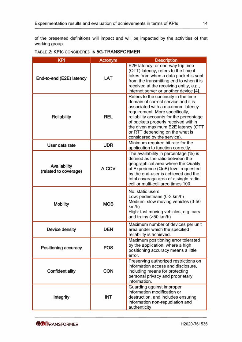
TABLE 2: KPIS CONSIDERED IN 5G-TRANSFORMER
KPI Acronym Description
End-to-end (E2E) latency LAT
E2E latency, or one-way trip time (OTT) latency, refers to the time it takes from when a data packet is sent from the transmitting end to when it is received at the receiving entity, e.g., internet server or another device [4].
Reliability REL
Refers to the continuity in the time domain of correct service and it is associated with a maximum latency requirement. More specifically, reliability accounts for the percentage of packets properly received within the given maximum E2E latency (OTT or RTT depending on the what is considered by the service).
User data rate UDR Minimum required bit rate for the application to function correctly.
Availability (related to coverage)
A-COV
The availability in percentage (%) is defined as the ratio between the geographical area where the Quality of Experience (QoE) level requested by the end-user is achieved and the total coverage area of a single radio cell or multi-cell area times 100.
Mobility MOB
No: static users Low: pedestrians (0-3 km/h) Medium: slow moving vehicles (3-50 km/h) High: fast moving vehicles, e.g. cars and trains (>50 km/h)
Device density DEN Maximum number of devices per unit area under which the specified reliability is achieved.
Positioning accuracy POS
Maximum positioning error tolerated by the application, where a high positioning accuracy means a little error.
Confidentiality CON
Preserving authorized restrictions on information access and disclosure, including means for protecting personal privacy and proprietary information.
Integrity INT
Guarding against improper information modification or destruction, and includes ensuring information non-repudiation and authenticity
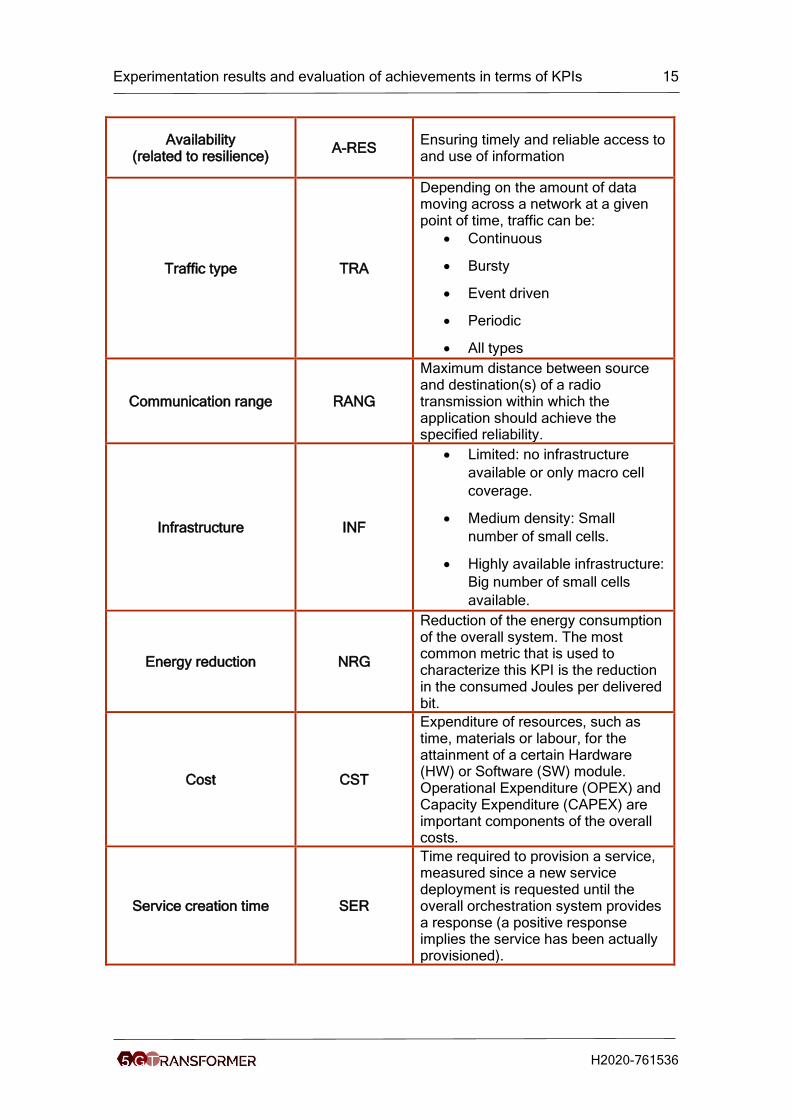
Experimentation results and evaluation of achievements in terms of KPIs 15
H2020-761536
Availability (related to resilience)
A-RES Ensuring timely and reliable access to and use of information
Traffic type TRA
Depending on the amount of data moving across a network at a given point of time, traffic can be:
• Continuous
• Bursty
• Event driven
• Periodic
• All types
Communication range RANG
Maximum distance between source and destination(s) of a radio transmission within which the application should achieve the specified reliability.
Infrastructure INF
• Limited: no infrastructure
available or only macro cell
coverage.
• Medium density: Small
number of small cells.
• Highly available infrastructure:
Big number of small cells
available.
Energy reduction NRG
Reduction of the energy consumption of the overall system. The most common metric that is used to characterize this KPI is the reduction in the consumed Joules per delivered bit.
Cost CST
Expenditure of resources, such as time, materials or labour, for the attainment of a certain Hardware (HW) or Software (SW) module. Operational Expenditure (OPEX) and Capacity Expenditure (CAPEX) are important components of the overall costs.
Service creation time SER
Time required to provision a service, measured since a new service deployment is requested until the overall orchestration system provides a response (a positive response implies the service has been actually provisioned).
Experimentation results and evaluation of achievements in terms of KPIs 16
H2020-761536
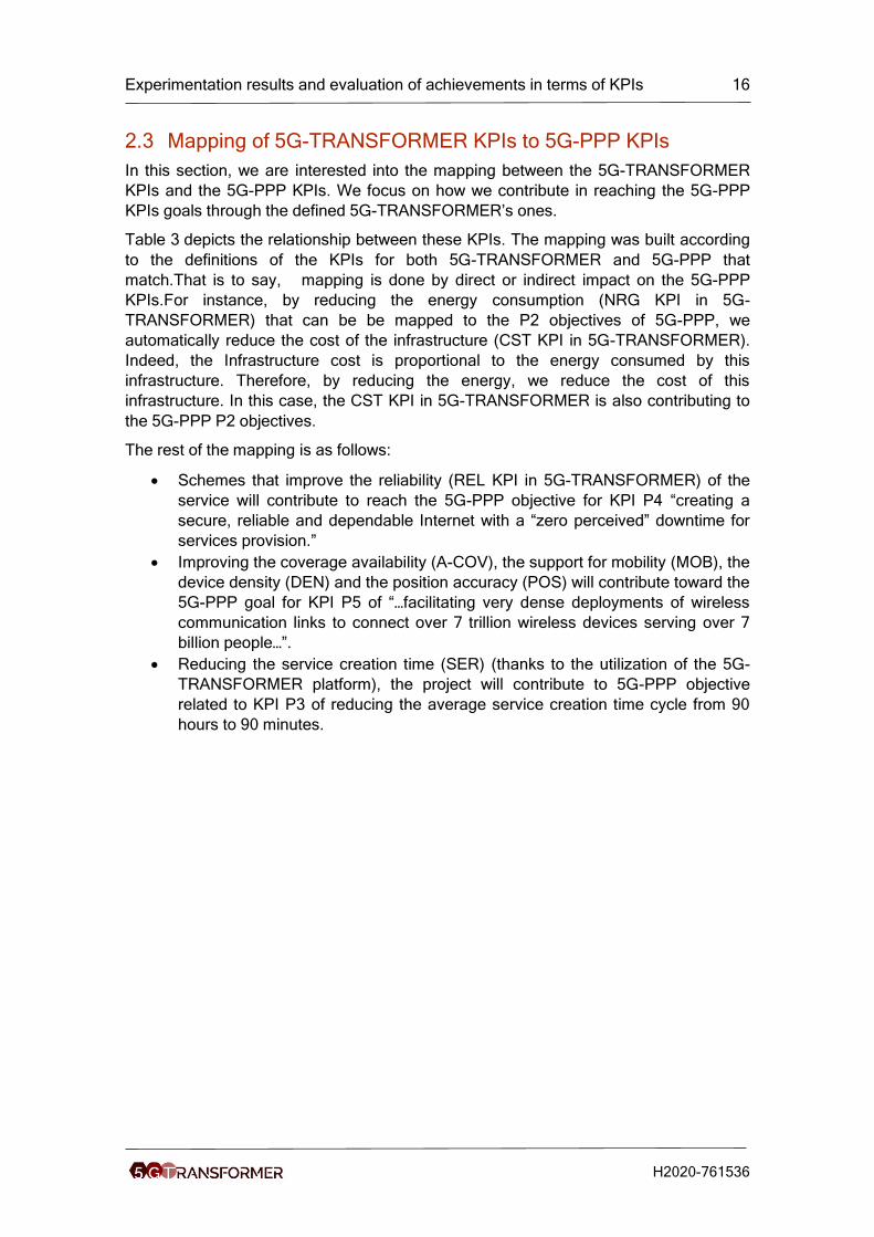
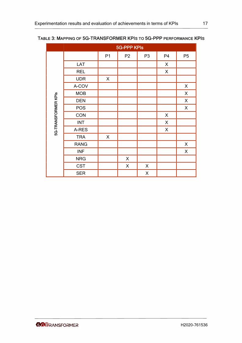
2.3 Mapping of 5G-TRANSFORMER KPIs to 5G-PPP KPIs
In this section, we are interested into the mapping between the 5G-TRANSFORMER
KPIs and the 5G-PPP KPIs. We focus on how we contribute in reaching the 5G-PPP
KPIs goals through the defined 5G-TRANSFORMER’s ones.
Table 3 depicts the relationship between these KPIs. The mapping was built according
to the definitions of the KPIs for both 5G-TRANSFORMER and 5G-PPP that
match.That is to say, mapping is done by direct or indirect impact on the 5G-PPP
KPIs.For instance, by reducing the energy consumption (NRG KPI in 5G-
TRANSFORMER) that can be be mapped to the P2 objectives of 5G-PPP, we
automatically reduce the cost of the infrastructure (CST KPI in 5G-TRANSFORMER).
Indeed, the Infrastructure cost is proportional to the energy consumed by this
infrastructure. Therefore, by reducing the energy, we reduce the cost of this
infrastructure. In this case, the CST KPI in 5G-TRANSFORMER is also contributing to
the 5G-PPP P2 objectives.
The rest of the mapping is as follows:
• Schemes that improve the reliability (REL KPI in 5G-TRANSFORMER) of the
service will contribute to reach the 5G-PPP objective for KPI P4 “creating a
secure, reliable and dependable Internet with a “zero perceived” downtime for
services provision.”
• Improving the coverage availability (A-COV), the support for mobility (MOB), the
device density (DEN) and the position accuracy (POS) will contribute toward the
5G-PPP goal for KPI P5 of “…facilitating very dense deployments of wireless
communication links to connect over 7 trillion wireless devices serving over 7
billion people…”.
• Reducing the service creation time (SER) (thanks to the utilization of the 5G-
TRANSFORMER platform), the project will contribute to 5G-PPP objective
related to KPI P3 of reducing the average service creation time cycle from 90
hours to 90 minutes.
Experimentation results and evaluation of achievements in terms of KPIs 17
H2020-761536
TABLE 3: MAPPING OF 5G-TRANSFORMER KPIS TO 5G-PPP PERFORMANCE KPIS
5G-PPP KPIs
5G
-TR
AN
SF
OR
ME
R K
PIs
P1 P2 P3 P4 P5
LAT X
REL X
UDR X
A-COV X
MOB X
DEN X
POS X
CON X
INT X
A-RES X
TRA X
RANG X
INF X
NRG X
CST X X
SER X
Experimentation results and evaluation of achievements in terms of KPIs 18
H2020-761536
3 Selected Proofs of Concept This section describes the selected proofs of concept that have been considered for
this initial evaluation.
3.1 Automotive
In D5.2 [1], we have described the procedure that has been implemented for the
selection of the use case that will be developed for the final PoC.
The Automotive PoC will demonstrate the EVS (Extended Virtual Sensing) use case
(UC), which emphasizes the use of external infrastructure for collecting the information
from vehicles, in order to calculate the probability of a collision on an intersection and, if
necessary, provide an emergency message to the driver. In addition to the EVS service
it will be added also video streaming service. The additional value is that the EVS
service will be stable and functional while a video streaming service is active onboard.
In particular, the 5G-TRANSFORMER functionalities will allow the automatic
deployment of EVS service for covering dangerous intersections and the scalability of
the EVS service components (based on the traffic in the monitored area) in order to
ensure the defined SLAs, also when running EVS service and Video Streaming Service
(that have different priorities) simultaneously.
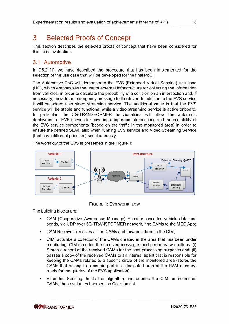
The workflow of the EVS is presented in the Figure 1:
FIGURE 1: EVS WORKFLOW
The building blocks are:
• CAM (Cooperative Awareness Message) Encoder: encodes vehicle data and
sends, via UDP over 5G-TRANSFORMER network, the CAMs to the MEC App;
• CAM Receiver: receives all the CAMs and forwards them to the CIM;
• CIM: acts like a collector of the CAMs created in the area that has been under
monitoring. CIM decodes the received messages and performs two actions: (i)
Stores a record of the received CAMs for the post-processing purposes and, (ii)
passes a copy of the received CAMs to an internal agent that is responsible for
keeping the CAMs related to a specific circle of the monitored area (stores the
CAMs that belong to a certain part in a dedicated area of the RAM memory,
ready for the queries of the EVS application).
• Extended Sensing: hosts the algorithm and queries the CIM for interested
CAMs, then evaluates Intersection Collision risk.
Experimentation results and evaluation of achievements in terms of KPIs 19
H2020-761536
• DENM Decider: triggered by Extended Sensing only in cases where the risk is
detected. Sends DENM messages to the vehicles involved in a potential
collision calculated by the ES algorithm.
• DENM Decoder: decodes the DENM received by the vehicle through the
modem
The interactions between described building blocks are following:
Vehicle 1 sends Cooperative Awareness Message (CAM) every 100ms, which includes
information related to its position, speed and direction. The vEPC receives the traffic
directed towards the CAM receiver. All CAMs are sent and stored in CIM, through the
CAM Receiver. Then Extended Sensing periodically queries the CIM for the latest
CAMs in the area of interest and calculates the probability of collision. If a risk is
detected, Extended Sensing invokes the DENM Decider that sends unicast alert
message (DENM) to alert vehicles involved in a course of a possible collision.
E2E latency is considered for the CAMs that trigger a warning and it is the time elapsed
since the encoded CAM is available at location A (inside the vehicle) till the time when
the decoded DENM is available at location R (𝑇𝐴�́�).
3.2 Entertainment
The Entertainment PoC aims to provide a video streaming service to deliver an
immersive and interactive experience to users attending a sports event. The
demonstration consists of two PoCs regarding On-site live experience (OLE) and Ultra
High-Definition (UHD) use cases foreseeing the streaming of UHD live feeds that can
be consumed on-demand by the users.
The objective of the demonstration is to prove that 5G-TRANSFORMER platform can
deploy a video service simultaneously to multiple users in the same or in different
locations. In this sense, 5G-TRANSFORMER platform can place the resources near
the users, ensuring the availability of the network and reducing significantly the end-to-
end latency of the network allowing a better experience to the fans in a sports venue.
These features are essential since the source feed of the video can be local to a venue
and the service must be able to provide the users an immersive experience by means
of an optimal use of the network infrastructure. The 5G-TRANSFORMER platform
allows the Entertainment vertical to instantiate the streaming service dynamically in
seconds, providing a transparent abstraction of the network infrastructure and auto-
scaling functionalities to manage different load conditions.
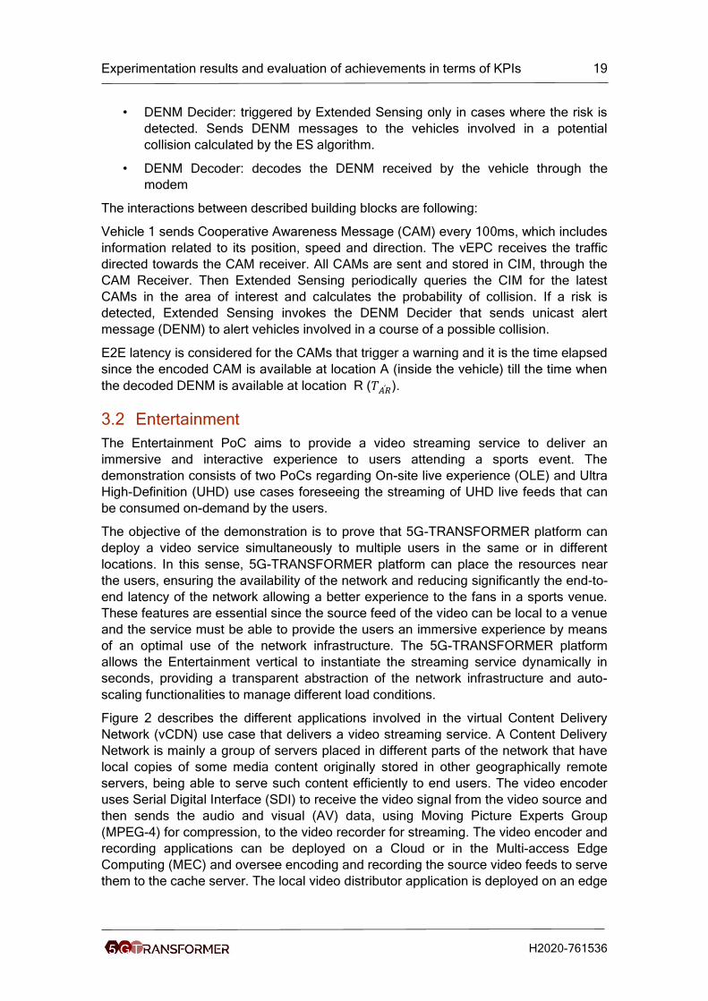
Figure 2 describes the different applications involved in the virtual Content Delivery
Network (vCDN) use case that delivers a video streaming service. A Content Delivery
Network is mainly a group of servers placed in different parts of the network that have
local copies of some media content originally stored in other geographically remote
servers, being able to serve such content efficiently to end users. The video encoder
uses Serial Digital Interface (SDI) to receive the video signal from the video source and
then sends the audio and visual (AV) data, using Moving Picture Experts Group
(MPEG-4) for compression, to the video recorder for streaming. The video encoder and
recording applications can be deployed on a Cloud or in the Multi-access Edge
Computing (MEC) and oversee encoding and recording the source video feeds to serve
them to the cache server. The local video distributor application is deployed on an edge
Experimentation results and evaluation of achievements in terms of KPIs 20
H2020-761536
cloud or in the MEC to be close to the users in order to validate user access and serve
the video feed from the video recorder to the users.
FIGURE 2: DESIGN OF OLE AND UHD USE CASES
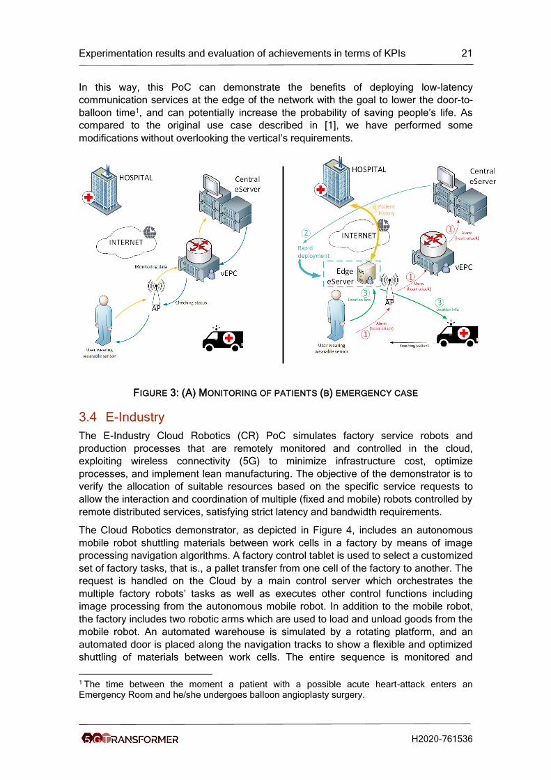
3.3 E-Health
D1.1 [2] describes the list of e-Health use cases considered in 5G-TRANSFORMER.
The heart-attack emergency use case from the listed E-Health use cases is selected for
demonstration. As depicted in Figure 3, the use case is composed of users wearing a
smart wearable device (e.g., smart shirt or smart watch) that can detect a potential
health issue (e.g., heart-attack, high blood pressure, etc.). The wearable periodically
reports the health status to a central server. If the monitoring data shows a potential
issue, the central server issues an alarm to the wearable device so the user can mark it
as a false alarm, or the issue will be confirmed if there is no feedback for certain
interval. In the case of a confirmed alarm (e.g., no feedback from the user), the central
server requests paramedics in the location of the user and requests deployment of an
edge service closer to the user. The edge service is deployed to lower the latency and
provide features to ambulances or patients (e.g., patient history, remote consultation,
video streaming, AR/VR features etc.). Once the edge service is deployed (on a host
close to the user), the edge application establishes a connection to the user’s hospital,
obtaining the health records and establishes a connection with the paramedic teams
that are involved in the emergency response. The paramedics can obtain the records
from the edge service or, in case it is needed, the paramedics can establish video
stream connection to a medical specialist (e.g., surgeon) located at a remote site (e.g.,
hospital far away from the emergency location) to perform remote surgery or
consultation through the edge service. The edge service can also be used as video
streaming hub to enable Augmented and Virtual Reality applications supporting the
emergency personnel deployed.
Experimentation results and evaluation of achievements in terms of KPIs 21
H2020-761536
In this way, this PoC can demonstrate the benefits of deploying low-latency
communication services at the edge of the network with the goal to lower the door-to-
balloon time1, and can potentially increase the probability of saving people’s life. As
compared to the original use case described in [1], we have performed some
modifications without overlooking the vertical’s requirements.
FIGURE 3: (A) MONITORING OF PATIENTS (B) EMERGENCY CASE
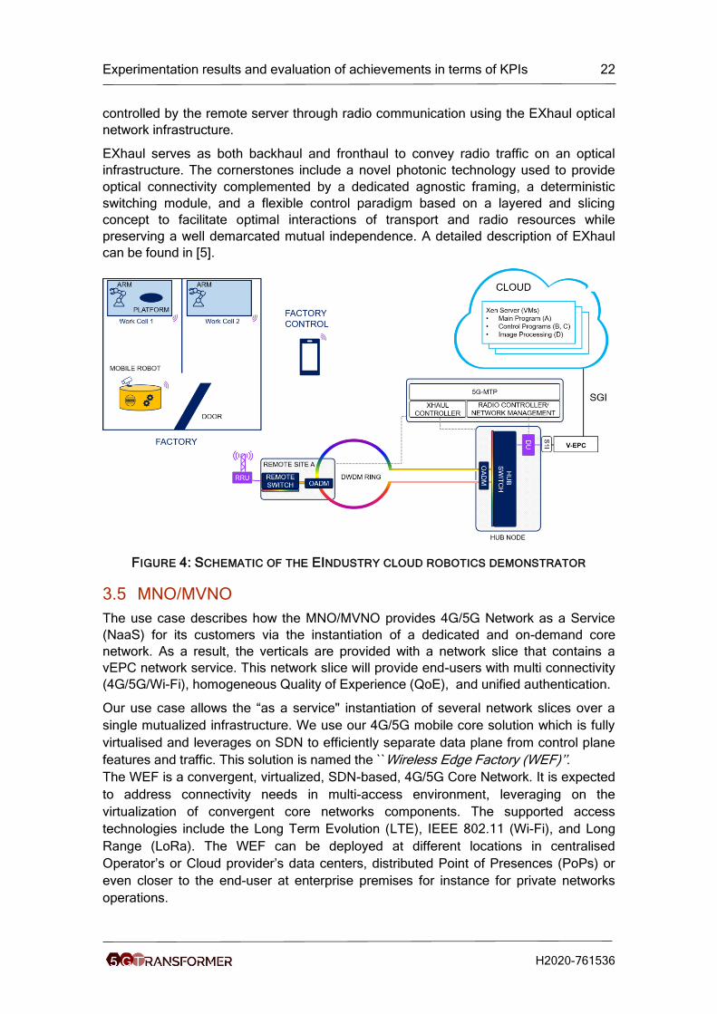
3.4 E-Industry
The E-Industry Cloud Robotics (CR) PoC simulates factory service robots and
production processes that are remotely monitored and controlled in the cloud,
exploiting wireless connectivity (5G) to minimize infrastructure cost, optimize
processes, and implement lean manufacturing. The objective of the demonstrator is to
verify the allocation of suitable resources based on the specific service requests to
allow the interaction and coordination of multiple (fixed and mobile) robots controlled by
remote distributed services, satisfying strict latency and bandwidth requirements.
The Cloud Robotics demonstrator, as depicted in Figure 4, includes an autonomous
mobile robot shuttling materials between work cells in a factory by means of image
processing navigation algorithms. A factory control tablet is used to select a customized
set of factory tasks, that is., a pallet transfer from one cell of the factory to another. The
request is handled on the Cloud by a main control server which orchestrates the
multiple factory robots’ tasks as well as executes other control functions including
image processing from the autonomous mobile robot. In addition to the mobile robot,
the factory includes two robotic arms which are used to load and unload goods from the
mobile robot. An automated warehouse is simulated by a rotating platform, and an
automated door is placed along the navigation tracks to show a flexible and optimized
shuttling of materials between work cells. The entire sequence is monitored and
1 The time between the moment a patient with a possible acute heart-attack enters an Emergency Room and he/she undergoes balloon angioplasty surgery.
Experimentation results and evaluation of achievements in terms of KPIs 22
H2020-761536
controlled by the remote server through radio communication using the EXhaul optical
network infrastructure.
EXhaul serves as both backhaul and fronthaul to convey radio traffic on an optical
infrastructure. The cornerstones include a novel photonic technology used to provide
optical connectivity complemented by a dedicated agnostic framing, a deterministic
switching module, and a flexible control paradigm based on a layered and slicing
concept to facilitate optimal interactions of transport and radio resources while
preserving a well demarcated mutual independence. A detailed description of EXhaul
can be found in [5].
FIGURE 4: SCHEMATIC OF THE EINDUSTRY CLOUD ROBOTICS DEMONSTRATOR
3.5 MNO/MVNO
The use case describes how the MNO/MVNO provides 4G/5G Network as a Service
(NaaS) for its customers via the instantiation of a dedicated and on-demand core
network. As a result, the verticals are provided with a network slice that contains a
vEPC network service. This network slice will provide end-users with multi connectivity
(4G/5G/Wi-Fi), homogeneous Quality of Experience (QoE), and unified authentication.
Our use case allows the “as a service" instantiation of several network slices over a
single mutualized infrastructure. We use our 4G/5G mobile core solution which is fully
virtualised and leverages on SDN to efficiently separate data plane from control plane
features and traffic. This solution is named the ``Wireless Edge Factory (WEF)’’.
The WEF is a convergent, virtualized, SDN-based, 4G/5G Core Network. It is expected
to address connectivity needs in multi-access environment, leveraging on the
virtualization of convergent core networks components. The supported access
technologies include the Long Term Evolution (LTE), IEEE 802.11 (Wi-Fi), and Long
Range (LoRa). The WEF can be deployed at different locations in centralised
Operator’s or Cloud provider’s data centers, distributed Point of Presences (PoPs) or
even closer to the end-user at enterprise premises for instance for private networks
operations.
Experimentation results and evaluation of achievements in terms of KPIs 23
H2020-761536
One of the main challenges is to evolve smoothly from current 4G core network
components to 5G. To this aim, the WEF release integrates an SDN based approach
directly in the EPC. In short, control plane components are virtualized, including the
WEF SDN controller which controls a programmable user plane distributed over
several virtual or physical SDN switches. The SDN based separation between the
control plane and the data plane brings the flexibility to host control plane VNFs in a
centralised Cloud while data plane VNFs being distributed at (or closed to) each access
site. It is hence foreseen that each access network (e.g., on different campus,
corporate agency, industrial site or factory) will leverage on distributed data plane
functions for efficient routing of users’ traffic, while being controlled from a single
control plane in the Cloud. Regarding the external interfaces, they are compliant with
legacy standards, especially the 3GPP interfaces to User Equipment (UE), RAN and
external Packet Data Network (PDN).
Most of the WEF core components are also compliant with the 3GPP standards. Only
the S/P-GW is reworked to follow the SDN model. Leveraging on such flexibility, user
Plane traffic is handled efficiently through flow table forwarding principles while the
control plane is managed in a centralized fashion with the SDN controller and its
northbound applications. The user plane is supported through the GW-U, whatever the
access technology is (such as, Wi-Fi and LTE). Several GW-U can be distributed on
different locations. They gather traffic to/from the access networks on the one hand and
the external network on the other hand. GW-U are based on virtual SDN switches that
have been modified to be able to cope with LTE access and 3GPP protocols. Thus,
they can be instantiated on servers with virtualization capabilities (e.g., KVM
hypervisor) or directly on bare-metal devices. Control plane functional entities are
embedding the SDN Controller that interacts, on its Southbound Interface, with several
GW-Us to control users’ traffic forwarding rules and, on its Northbound Interface, with
S/PGW-C coming as an SDN application to handle the S/PGW logic for users’ traffic
handling. The S/PGW-C application interacts with the MME as if it was a legacy
monolithic S/PGW. Following 3GPP standards, the MME is also interfaced with the
HSS for subscriber’s authentication as well as, on the access side, with eNodeBs and
UEs. The AAA server brings the Subscriber Identity Module (SIM) based authentication
support for Wi-Fi users, interacting with the HSS (non-3GPP access interworking in
trusted mode is supported). Dynamic address allocation is hand through a DHCP
server while a legacy NAT allows private IP addressing and its mapping with external
networks. Lastly, Service Function Chaining (SFC) features allow handling data
packets redirection through a given and ordered set of VNFs in the user plane.
Whatever the access technology used, the WEF provides unified access authorization,
user’s authentication, and IP address allocation, which enables to deliver users’ traffic
with various policies regardless the used access network. In our experiment, the WEF
is instantiated in a network slice to (i) manage Wi-Fi and 4G access infrastructure built
from standard equipment with multiple RAN access points per site (evolved NodeB
(eNB) and Wi-Fi access point); (ii) unify subscribers management, authentication, IP
addressing and security over the different technologies; (iii) provide efficient local users
traffic switching policy capabilities thanks to the complete separation between the
control plane and the user plane; (iv) be deploy-able as VNFs in off-theshelf server.
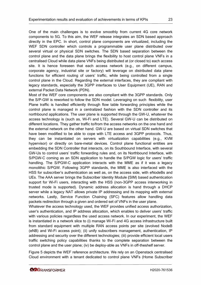
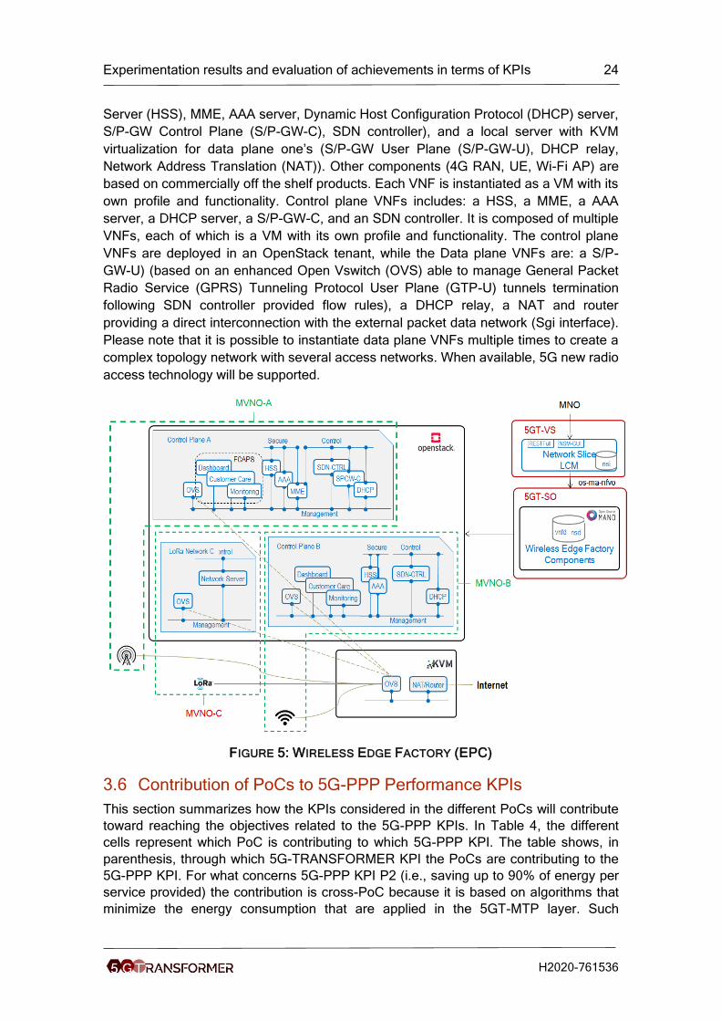
Figure 5 depicts the WEF reference architecture. We rely on an Openstack centralised
Cloud environment with a tenant dedicated to control plane VNFs (Home Subscriber
Experimentation results and evaluation of achievements in terms of KPIs 24
H2020-761536
Server (HSS), MME, AAA server, Dynamic Host Configuration Protocol (DHCP) server,
S/P-GW Control Plane (S/P-GW-C), SDN controller), and a local server with KVM
virtualization for data plane one’s (S/P-GW User Plane (S/P-GW-U), DHCP relay,
Network Address Translation (NAT)). Other components (4G RAN, UE, Wi-Fi AP) are
based on commercially off the shelf products. Each VNF is instantiated as a VM with its
own profile and functionality. Control plane VNFs includes: a HSS, a MME, a AAA
server, a DHCP server, a S/P-GW-C, and an SDN controller. It is composed of multiple
VNFs, each of which is a VM with its own profile and functionality. The control plane
VNFs are deployed in an OpenStack tenant, while the Data plane VNFs are: a S/P-
GW-U) (based on an enhanced Open Vswitch (OVS) able to manage General Packet
Radio Service (GPRS) Tunneling Protocol User Plane (GTP-U) tunnels termination
following SDN controller provided flow rules), a DHCP relay, a NAT and router
providing a direct interconnection with the external packet data network (Sgi interface).
Please note that it is possible to instantiate data plane VNFs multiple times to create a
complex topology network with several access networks. When available, 5G new radio
access technology will be supported.
FIGURE 5: WIRELESS EDGE FACTORY (EPC)
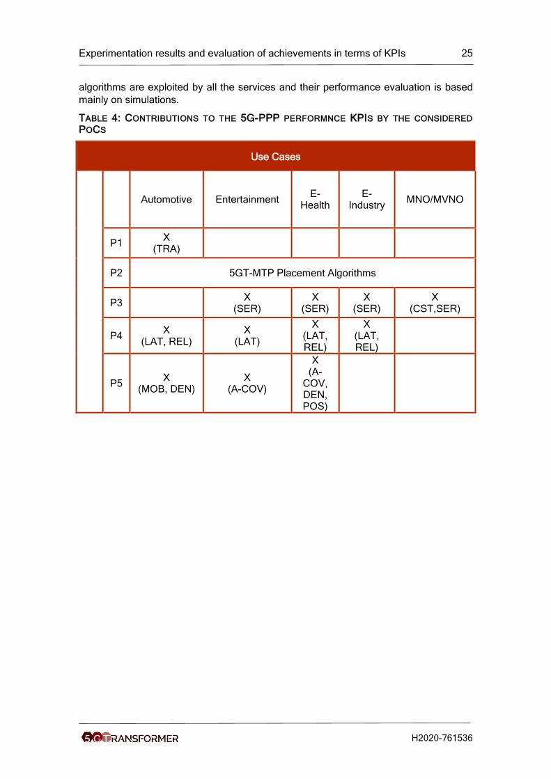
3.6 Contribution of PoCs to 5G-PPP Performance KPIs
This section summarizes how the KPIs considered in the different PoCs will contribute
toward reaching the objectives related to the 5G-PPP KPIs. In Table 4, the different
cells represent which PoC is contributing to which 5G-PPP KPI. The table shows, in
parenthesis, through which 5G-TRANSFORMER KPI the PoCs are contributing to the
5G-PPP KPI. For what concerns 5G-PPP KPI P2 (i.e., saving up to 90% of energy per
service provided) the contribution is cross-PoC because it is based on algorithms that
minimize the energy consumption that are applied in the 5GT-MTP layer. Such
Experimentation results and evaluation of achievements in terms of KPIs 25
H2020-761536
algorithms are exploited by all the services and their performance evaluation is based
mainly on simulations.
TABLE 4: CONTRIBUTIONS TO THE 5G-PPP PERFORMNCE KPIS BY THE CONSIDERED
POCS
Use Cases
5G
-PP
P K
PIs
Automotive Entertainment E-
Health E-
Industry MNO/MVNO
P1 X
(TRA)
P2 5GT-MTP Placement Algorithms
P3 X (SER)
X (SER)
X (SER)
X (CST,SER)
P4 X
(LAT, REL) X
(LAT)
X (LAT, REL)
X (LAT, REL)
P5 X
(MOB, DEN) X
(A-COV)
X (A-
COV, DEN, POS)
Experimentation results and evaluation of achievements in terms of KPIs 26
H2020-761536
4 Experiments, Measurements, Results The aim of this section is to evaluate the components developed in the different WPs
(WP2, WP3, and WP4) by performing simulations and experimentations of the PoCs.
Therefore, through this section, we would like to know whether these components are
capable to meet the expected KPIs required by the verticals. These KPIs will be
compared with state of art solutions already proposed in the literature or used in the
common practice to evaluate whether the 5G-TRANSFORMER platform is enhancing
these KPIs.
Through this section, we point out for each of the selected use cases, the considered
KPIs, the description of the performed experiments, with the measurements and the
obtained results.
4.1 Automotive
4.1.1 Considered KPI(s) and benchmark
For the Automotive UC, the highlighted KPIs are: Latency (LAT), Reliability (REL),
Density (DEN), Traffic (TRA), and Mobility (MOB):
• LAT: Measuring the whole service workflow (from generating and sending the
CAM by the vehicle, to receiving back the DENM message).
• REL: Measuring the percentage of messages that have been sent and received
correctly.
• DEN: Measuring the maximum number of vehicles in a considered area, where
reliability is higher than 99 percent.
• TRA: Measuring the amount of data transmitted from and to the vehicles.
• MOB: Measuring the correct functionality of the service, considering different
car speeds (higher than 50 km/h).
The timeline for the KPI measurements is presented in [1]. Initial measurements are
done for LAT, REL and DEN. It is important to highlight that before introducing the
video streaming service (planned for the PoC1.4), the DEN and TRA KPIs are
correlated, since the number of sent CAMs per second is fixed.
For the Benchmarking of the considered KPIs, it is important to provide a brief overview
of the technologies that can be used for the vehicular communications. Up until few
years ago, the only standard for vehicular communications (which enables cooperative
awareness) was Wireless Access in the Vehicular Environment (WAVE), based on
IEEE 802.11p [28] [29] in the U.S. and the corresponding Cooperative Intelligent
Transport System (C-ITS) based on ITS-G5 in Europe [30]. Regarding the cooperative
awareness service, WAVE has introduced Basic Safety Message (BSM), while ETSI
has introduced the Cooperative Awareness Message (CAM) as basic service [31].
On the other side, in the last few years the stakeholders have been investigating the
usability of the cellular network to support vehicular applications. There have been
published several comparisons between the two competitor technologies, IEEE
802.11p and LTE network (non V2V), for the vehicular applications [32].
In [33], both standards are compared in terms of reliability, latency and mobility, which
are the requirements highlighted for the automotive application in 5G-TRANSFORMER.
Experimentation results and evaluation of achievements in terms of KPIs 27
H2020-761536
The mentioned performance comparisons highlight the LTE as the technology with
superior network capacity with respect to 802.11p, also affected by more reliable
transmissions.
The selection of the best technology for vehicular applications is still under intense
debate.
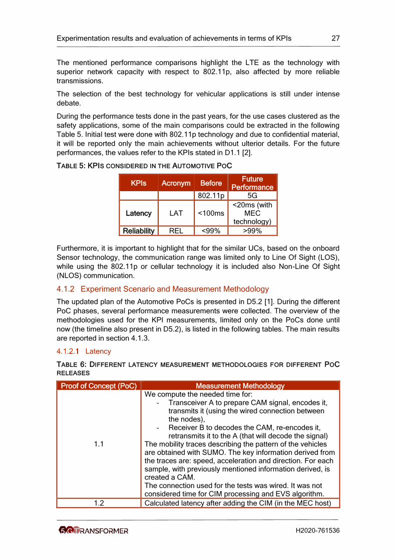
During the performance tests done in the past years, for the use cases clustered as the
safety applications, some of the main comparisons could be extracted in the following
Table 5. Initial test were done with 802.11p technology and due to confidential material,
it will be reported only the main achievements without ulterior details. For the future
performances, the values refer to the KPIs stated in D1.1 [2].
TABLE 5: KPIS CONSIDERED IN THE AUTOMOTIVE POC
KPIs Acronym Before Future
Performance 802.11p 5G
Latency LAT <100ms <20ms (with
MEC technology)
Reliability REL <99% >99%
Furthermore, it is important to highlight that for the similar UCs, based on the onboard
Sensor technology, the communication range was limited only to Line Of Sight (LOS),
while using the 802.11p or cellular technology it is included also Non-Line Of Sight
(NLOS) communication.
4.1.2 Experiment Scenario and Measurement Methodology
The updated plan of the Automotive PoCs is presented in D5.2 [1]. During the different
PoC phases, several performance measurements were collected. The overview of the
methodologies used for the KPI measurements, limited only on the PoCs done until
now (the timeline also present in D5.2), is listed in the following tables. The main results
are reported in section 4.1.3.
Latency
TABLE 6: DIFFERENT LATENCY MEASUREMENT METHODOLOGIES FOR DIFFERENT POC
RELEASES
Proof of Concept (PoC) Measurement Methodology
1.1
We compute the needed time for: - Transceiver A to prepare CAM signal, encodes it,
transmits it (using the wired connection between the nodes),
- Receiver B to decodes the CAM, re-encodes it, retransmits it to the A (that will decode the signal)
The mobility traces describing the pattern of the vehicles are obtained with SUMO. The key information derived from the traces are: speed, acceleration and direction. For each sample, with previously mentioned information derived, is created a CAM. The connection used for the tests was wired. It was not considered time for CIM processing and EVS algorithm.
1.2 Calculated latency after adding the CIM (in the MEC host)
Experimentation results and evaluation of achievements in terms of KPIs 28
H2020-761536
that receives and processes CAMs from the vehicle and the traffic simulator in the selected area. CIM performs the following actions: it is responsible for storing the record of all received CAMs in a PostgreSQL Database (for post-processing purposes), and contemporarily it switches the received CAMs to each CAM Manager according to their monitored area. In other words, when CAMs are passed to the CAM Manager, it is verified if they are belonging to the same predefined area of interest and then, consequently, stored into the corresponding dedicated area of RAM memory.
1.2+ Calculated channel latency with real radio equipment.
1.3
Calculated E2E latency after adding the EVS algorithm. The E2E delay is computed only on the CAMs that trigger a DENM, since it is the time that elapses between the transmission of a CAM by a vehicle and the reception (on the same vehicle) of the DENM triggered by such a CAM.
1.4
Ongoing measurements and performance improvements for each software component. After the modifications of the CIM, EVS algorithm and DENM Decider (in order to gain better performances respect to the results obtained in PoC 1.3), the ongoing measurements are including the following actions: The mobility traces of each vehicle are sampled every 0,1 second. CAMs are transmitted from the UEs towards the eNodeB of the Open air interface (OAI) cellular network. The EVS application queries the latest CAMs from the CIM, every 5ms, through the TCP connection. When the CAMs are provided, the algorithm checks if there is a rick of a collision. If EVS detects the risk, it triggers the DENM Decider that sends, via UDP over the network, a unicast alert message (DENM) to the vehicles which CAMs have triggered the warning.
Reliability
TABLE 7: DIFFERENT RELIABILITY MEASUREMENT METHODOLOGIES FOR DIFFEERENT
POC RELEASES
Proof of Concept (PoC) Measurement Methodology
1.1
SimuLTE-Veins [34] is a framework for simulating cellular communication in vehicular networks (C-V2X communications). It is based on Simulation of Urban Mobility (SUMO) [35] tool. During the first phase, it is used this tool in order to simulate several road traffic scenarios. In particular, two vehicles flowing in an urban environment. The map on which vehicles move is composed of three roads, one horizontal (1300m-long) and two vertical (800m-long) with a single lane per direction. The two vertical roads intersect the horizontal one in two points, creating two crossroads where vehicles can collide. Vehicles periodically send CAMs to the eNB. Then a DENM is generated and sent back to the vehicles. From each simulation are
Experimentation results and evaluation of achievements in terms of KPIs 29
H2020-761536
mainly got two files: a CAM log and a DENM log. With these two files it is possible to prepare a CAM trace and a DENM trace for the test-bed. The CAM trace is read by the OAI UE, which forwards CAMs towards the eNB. The OAI eNB receives these message and forwards them to the MEC host. DENMs are generated by the MEC host and do the opposite path. At this point it is calculated how many DENMs have been sent and received (in PoC1.1, OAI UE and OAI eNodeB are connected via wire). Measurements are done using the following parameters:
• 30 simulations with SimuLTE-Veins; in each simulation 2 vehicles are simulated
• Each simulation lasted around 60 seconds • With the CAM log and DENM log of the
SimuLTE-Veins simulations, it was generated the corresponding CAM and DENM trace
At the end of their process, computing the DENM PSR (Packet Success Rate).
1.2 Calculated the reliability of each software component.
1.3 – 1.4
Performance improvements of each software component. In the latest tests done the focus was more on the results from the report on the CAMs transmitted by the Vehicle Simulator - CAMs received from the CAM Receiver, than on DENMs (which are not many compared to the transmitted CAMs). Performance results are reported in Section 4.1.3.
Density
TABLE 8: DIFFERENT DENSITY MEASUREMENT METHODOLOGIES FOR DIFFERENT POC
RELEASES
Proof of Concept (PoC)
Measurement Methodology
1.1 - 1.4
Considered different vehicle density rates. The generation rate of vehicles is according a Poisson process with parameter λ; the higher is the value assumed by λ and the higher is the number of vehicles in the scenario. In order to know the vehicle density in the scenario, it is used SUMO (an open-source and very popular road traffic simulator).
• For each lambda were prepared 10 traces. Each SUMO input trace is an XML file describing the vehicles (e.g., max speed, max acceleration) and the path they will follow (i.e., the roads that will have to travel). The map is the same used for PoC 1.1; it is composed of three roads, one horizontal (1300m-long) and two vertical (800m-long) with a single lane per direction. Vehicles simulated never turn at the intersection, so they follow straight trajectories. The main vehicles’ parameters are the following:
◦ Length: 4.3 m
◦ Width: 1.8 m
Experimentation results and evaluation of achievements in terms of KPIs 30
H2020-761536
◦ Maximum speed: 13.89m/s (i.e., 50km/h)
◦ Acceleration: 4.5m/s2
• For each input trace it is used SUMO simulation
• SUMO produces many simulation output files. One of them, called “Summary” contains the simulation-wide number of vehicles that are loaded, inserted, running, waiting to be inserted, have reached their destination and how long they needed to finish the route. So, through such a file, it is possible to know for each simulation time-step (set to 100ms) the average number of vehicles in the scenario.
4.1.3 Results
Initially, in the PoC1.1 (also described in section 4.1.2.1) the scenario was following:
• UE PM applications (one of them is simulated and implemented as the MEC
VM) transmit CAMs of fixed size (57 bytes) to the MEC VM Application (running
EVS algorithm);
• MEC VM Application (EVS algorithm), transmits a set of DENMs, spreading
them between the two destinations which are transmitting CAMs at the same
time.
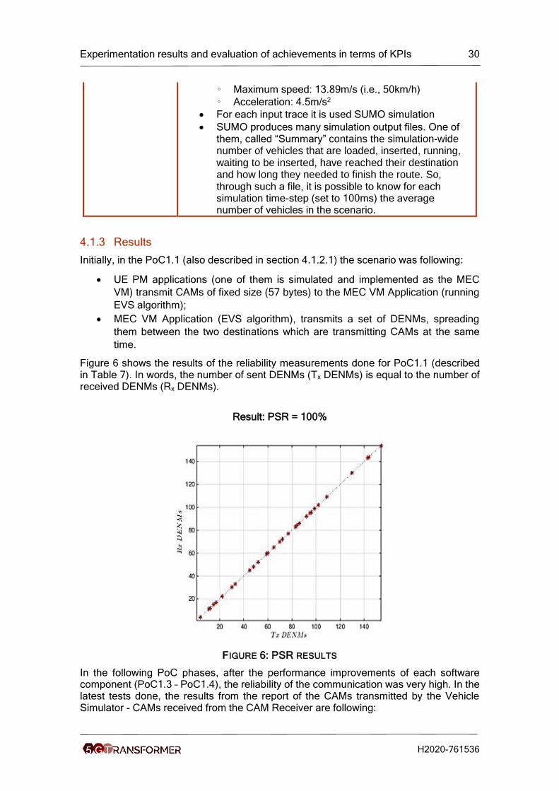
Figure 6 shows the results of the reliability measurements done for PoC1.1 (described in Table 7). In words, the number of sent DENMs (Tx DENMs) is equal to the number of received DENMs (Rx DENMs).
Result: PSR = 100%
FIGURE 6: PSR RESULTS
In the following PoC phases, after the performance improvements of each software component (PoC1.3 – PoC1.4), the reliability of the communication was very high. In the latest tests done, the results from the report of the CAMs transmitted by the Vehicle Simulator - CAMs received from the CAM Receiver are following:
Experimentation results and evaluation of achievements in terms of KPIs 31
H2020-761536
With the communication with a single UE connected on-air with OAI, a probability of loss (PLOSS) of the package (CAM) is around 0.002-0.005%.
Result: PLOSS = 0.002 – 0.005%
It was considered also different vehicle densities: 7 vehicles/km, 14 vehicles/km and 20 vehicles/km. For each of the three cases, five tests were done. The focus was on the following metrics:
• The time needed for the EVS to complete the following operations: o Query CAMs to the CIM; o update its internal tables with the new information received in the CAMs; o run the collision detector algorithm to detect possible collisions between
who sent the new CAMs and all the other vehicles known; o if a possible collision is detected, a DENM is prepared for the vehicles
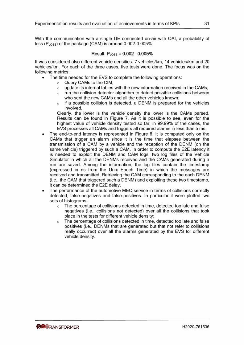
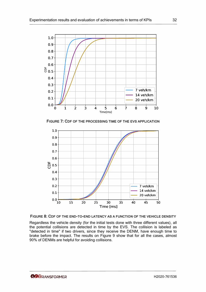
involved. Clearly, the lower is the vehicle density the lower is the CAMs parsed. Results can be found in Figure 7. As it is possible to see, even for the highest value of vehicle density tested so far, in 99.99% of the cases, the EVS processes all CAMs and triggers all required alarms in less than 5 ms;
• The end-to-end latency is represented in Figure 8. It is computed only on the CAMs that trigger an alarm since it is the time that elapses between the transmission of a CAM by a vehicle and the reception of the DENM (on the same vehicle) triggered by such a CAM. In order to compute the E2E latency it is needed to exploit the DENM and CAM logs, two log files of the Vehicle Simulator in which all the DENMs received and the CAMs generated during a run are saved. Among the information, the log files contain the timestamp (expressed in ns from the Unix Epoch Time) in which the messages are received and transmitted. Retrieving the CAM corresponding to the each DENM (i.e., the CAM that triggered such a DENM) and exploiting these two timestamp, it can be determined the E2E delay.
• The performance of the automotive MEC service in terms of collisions correctly detected, false-negatives and false-positives. In particular it were plotted two sets of histograms:
o The percentage of collisions detected in time, detected too late and false negatives (i.e., collisions not detected) over all the collisions that took place in the tests for different vehicle density;
o The percentage of collisions detected in time, detected too late and false positives (i.e., DENMs that are generated but that not refer to collisions really occurred) over all the alarms generated by the EVS for different vehicle density.
Experimentation results and evaluation of achievements in terms of KPIs 32
H2020-761536
FIGURE 7: CDF OF THE PROCESSING TIME OF THE EVS APPLICATION
FIGURE 8: CDF OF THE END-TO-END LATENCY AS A FUNCTION OF THE VEHICLE DENSITY
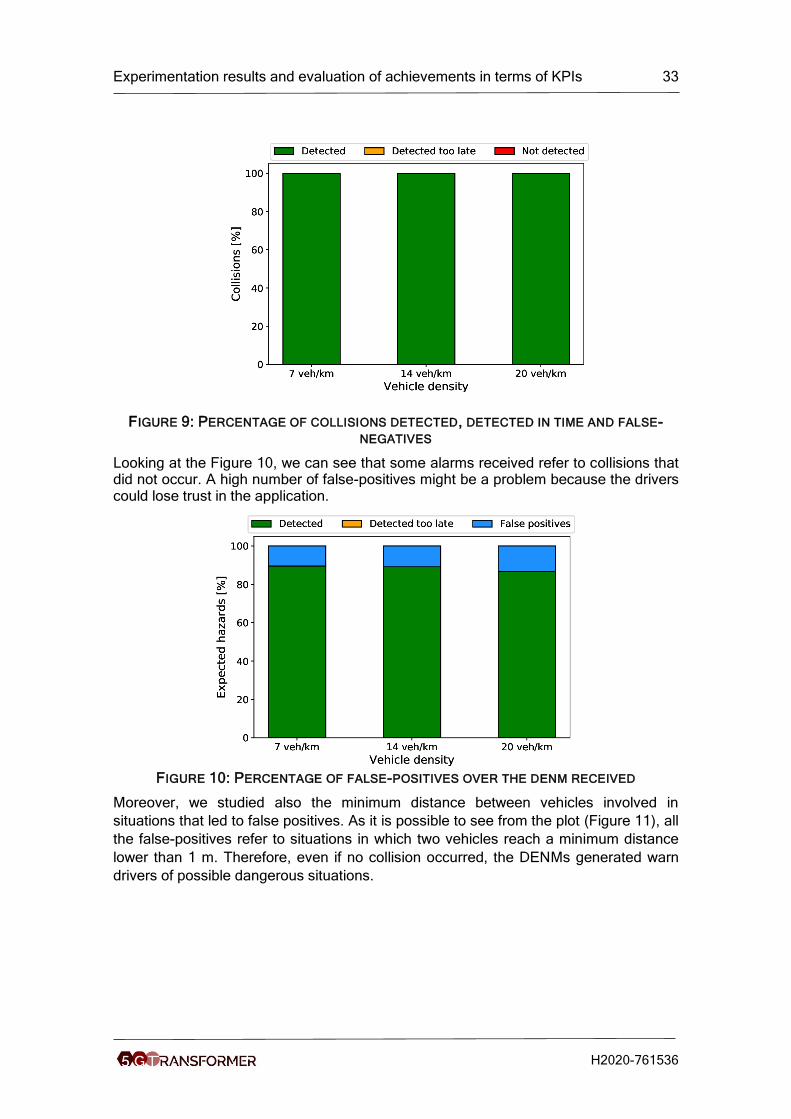
Regardless the vehicle density (for the initial tests done with three different values), all the potential collisions are detected in time by the EVS. The collision is labeled as "detected in time" if two drivers, since they receive the DENM, have enough time to brake before the impact. The results on Figure 9 show that for all the cases, almost 90% of DENMs are helpful for avoiding collisions.
Experimentation results and evaluation of achievements in terms of KPIs 33
H2020-761536
FIGURE 9: PERCENTAGE OF COLLISIONS DETECTED, DETECTED IN TIME AND FALSE-
NEGATIVES
Looking at the Figure 10, we can see that some alarms received refer to collisions that did not occur. A high number of false-positives might be a problem because the drivers could lose trust in the application.
FIGURE 10: PERCENTAGE OF FALSE-POSITIVES OVER THE DENM RECEIVED
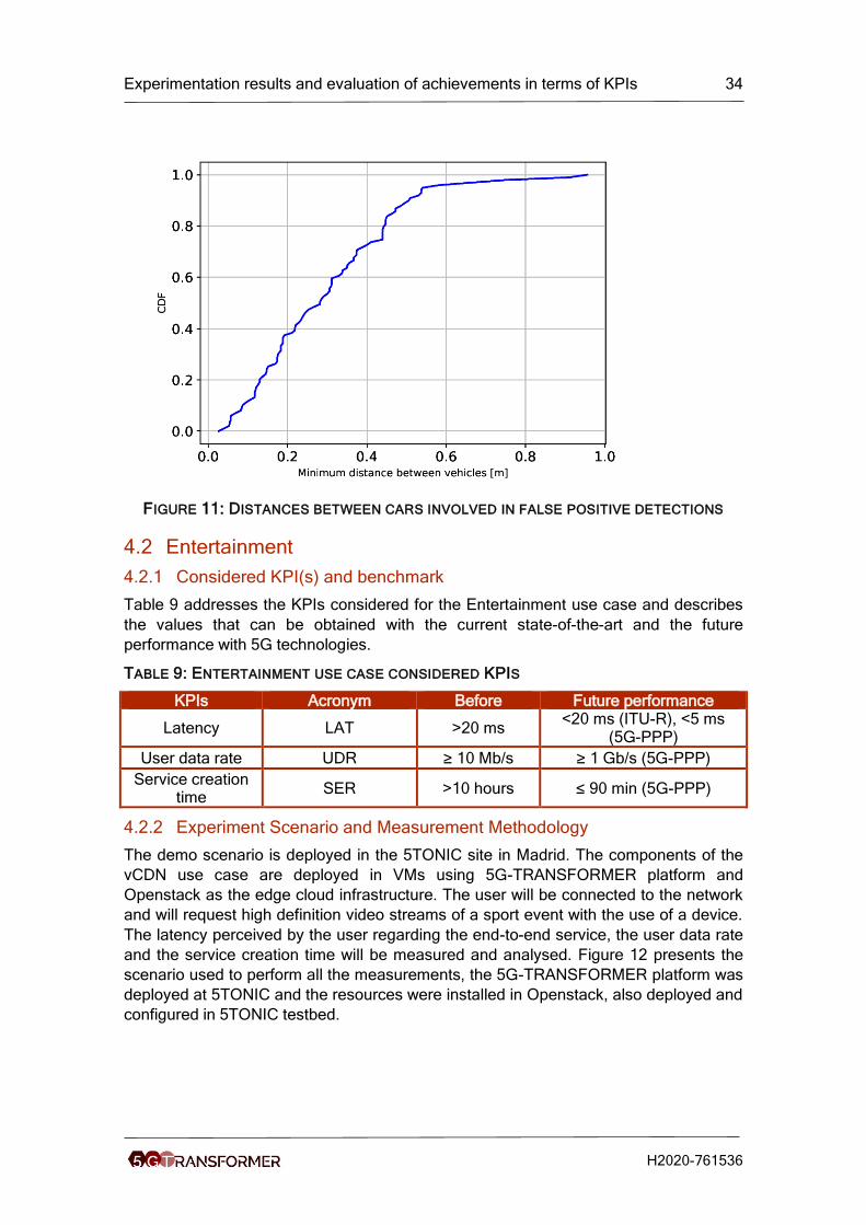
Moreover, we studied also the minimum distance between vehicles involved in
situations that led to false positives. As it is possible to see from the plot (Figure 11), all
the false-positives refer to situations in which two vehicles reach a minimum distance
lower than 1 m. Therefore, even if no collision occurred, the DENMs generated warn
drivers of possible dangerous situations.
Experimentation results and evaluation of achievements in terms of KPIs 34
H2020-761536
FIGURE 11: DISTANCES BETWEEN CARS INVOLVED IN FALSE POSITIVE DETECTIONS
4.2 Entertainment
4.2.1 Considered KPI(s) and benchmark
Table 9 addresses the KPIs considered for the Entertainment use case and describes
the values that can be obtained with the current state-of-the-art and the future
performance with 5G technologies.
TABLE 9: ENTERTAINMENT USE CASE CONSIDERED KPIS
KPIs Acronym Before Future performance
Latency LAT >20 ms <20 ms (ITU-R), <5 ms
(5G-PPP)
User data rate UDR ≥ 10 Mb/s ≥ 1 Gb/s (5G-PPP)
Service creation time
SER >10 hours ≤ 90 min (5G-PPP)
4.2.2 Experiment Scenario and Measurement Methodology
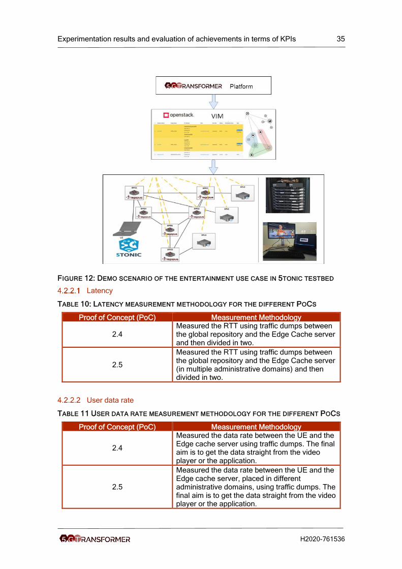
The demo scenario is deployed in the 5TONIC site in Madrid. The components of the
vCDN use case are deployed in VMs using 5G-TRANSFORMER platform and
Openstack as the edge cloud infrastructure. The user will be connected to the network
and will request high definition video streams of a sport event with the use of a device.
The latency perceived by the user regarding the end-to-end service, the user data rate
and the service creation time will be measured and analysed. Figure 12 presents the
scenario used to perform all the measurements, the 5G-TRANSFORMER platform was
deployed at 5TONIC and the resources were installed in Openstack, also deployed and
configured in 5TONIC testbed.
Experimentation results and evaluation of achievements in terms of KPIs 35
H2020-761536
FIGURE 12: DEMO SCENARIO OF THE ENTERTAINMENT USE CASE IN 5TONIC TESTBED
Latency
TABLE 10: LATENCY MEASUREMENT METHODOLOGY FOR THE DIFFERENT POCS
Proof of Concept (PoC) Measurement Methodology
2.4 Measured the RTT using traffic dumps between the global repository and the Edge Cache server and then divided in two.
2.5
Measured the RTT using traffic dumps between the global repository and the Edge Cache server (in multiple administrative domains) and then divided in two.
User data rate
TABLE 11 USER DATA RATE MEASUREMENT METHODOLOGY FOR THE DIFFERENT POCS
Proof of Concept (PoC) Measurement Methodology
2.4
Measured the data rate between the UE and the Edge cache server using traffic dumps. The final aim is to get the data straight from the video player or the application.
2.5
Measured the data rate between the UE and the Edge cache server, placed in different administrative domains, using traffic dumps. The final aim is to get the data straight from the video player or the application.
Experimentation results and evaluation of achievements in terms of KPIs 36
H2020-761536
Service creation time
TABLE 12 SERVICE CREATION TIME MEASUREMENT METHODOLOGY
Proof of Concept (PoC) Measurement Methodology
2.1 Measured the creation and configuration time of the Edge cache server and webserver, considering the 5GT-VS and the 5GT-SO.
4.2.3 Results
Latency
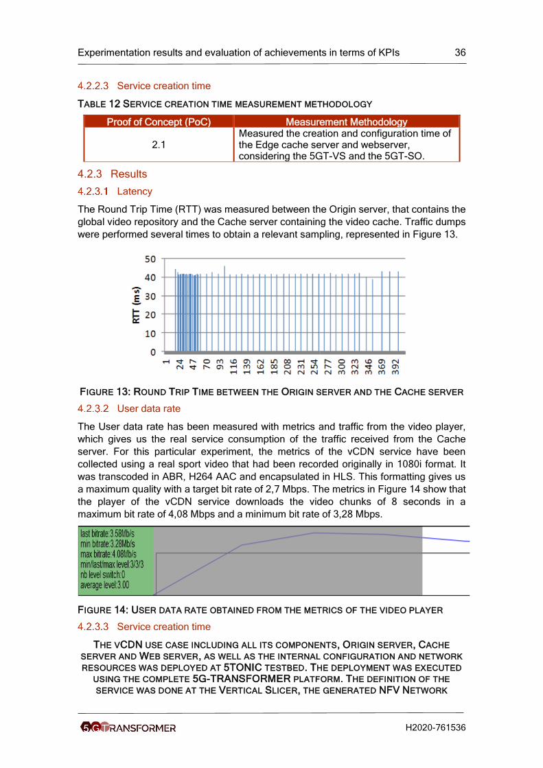
The Round Trip Time (RTT) was measured between the Origin server, that contains the
global video repository and the Cache server containing the video cache. Traffic dumps
were performed several times to obtain a relevant sampling, represented in Figure 13.
FIGURE 13: ROUND TRIP TIME BETWEEN THE ORIGIN SERVER AND THE CACHE SERVER
User data rate
The User data rate has been measured with metrics and traffic from the video player,
which gives us the real service consumption of the traffic received from the Cache
server. For this particular experiment, the metrics of the vCDN service have been
collected using a real sport video that had been recorded originally in 1080i format. It
was transcoded in ABR, H264 AAC and encapsulated in HLS. This formatting gives us
a maximum quality with a target bit rate of 2,7 Mbps. The metrics in Figure 14 show that
the player of the vCDN service downloads the video chunks of 8 seconds in a
maximum bit rate of 4,08 Mbps and a minimum bit rate of 3,28 Mbps.
FIGURE 14: USER DATA RATE OBTAINED FROM THE METRICS OF THE VIDEO PLAYER
Service creation time
THE VCDN USE CASE INCLUDING ALL ITS COMPONENTS, ORIGIN SERVER, CACHE
SERVER AND WEB SERVER, AS WELL AS THE INTERNAL CONFIGURATION AND NETWORK
RESOURCES WAS DEPLOYED AT 5TONIC TESTBED. THE DEPLOYMENT WAS EXECUTED
USING THE COMPLETE 5G-TRANSFORMER PLATFORM. THE DEFINITION OF THE
SERVICE WAS DONE AT THE VERTICAL SLICER, THE GENERATED NFV NETWORK
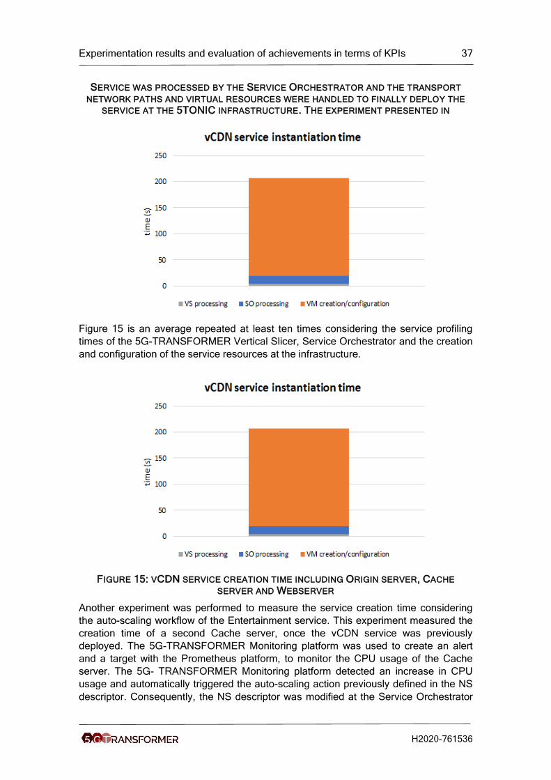
Experimentation results and evaluation of achievements in terms of KPIs 37
H2020-761536
SERVICE WAS PROCESSED BY THE SERVICE ORCHESTRATOR AND THE TRANSPORT
NETWORK PATHS AND VIRTUAL RESOURCES WERE HANDLED TO FINALLY DEPLOY THE
SERVICE AT THE 5TONIC INFRASTRUCTURE. THE EXPERIMENT PRESENTED IN
Figure 15 is an average repeated at least ten times considering the service profiling
times of the 5G-TRANSFORMER Vertical Slicer, Service Orchestrator and the creation
and configuration of the service resources at the infrastructure.
FIGURE 15: VCDN SERVICE CREATION TIME INCLUDING ORIGIN SERVER, CACHE
SERVER AND WEBSERVER
Another experiment was performed to measure the service creation time considering
the auto-scaling workflow of the Entertainment service. This experiment measured the
creation time of a second Cache server, once the vCDN service was previously
deployed. The 5G-TRANSFORMER Monitoring platform was used to create an alert
and a target with the Prometheus platform, to monitor the CPU usage of the Cache
server. The 5G- TRANSFORMER Monitoring platform detected an increase in CPU
usage and automatically triggered the auto-scaling action previously defined in the NS
descriptor. Consequently, the NS descriptor was modified at the Service Orchestrator
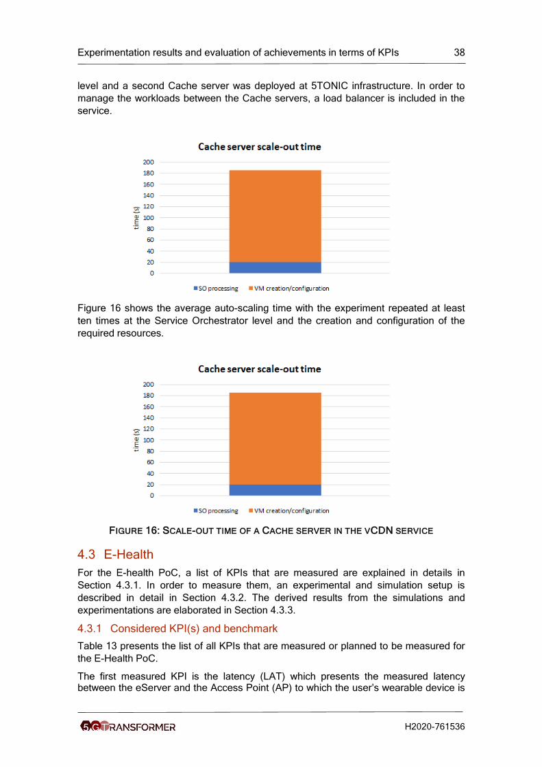
Experimentation results and evaluation of achievements in terms of KPIs 38
H2020-761536
level and a second Cache server was deployed at 5TONIC infrastructure. In order to
manage the workloads between the Cache servers, a load balancer is included in the
service.
Figure 16 shows the average auto-scaling time with the experiment repeated at least
ten times at the Service Orchestrator level and the creation and configuration of the
required resources.
FIGURE 16: SCALE-OUT TIME OF A CACHE SERVER IN THE VCDN SERVICE
4.3 E-Health
For the E-health PoC, a list of KPIs that are measured are explained in details in
Section 4.3.1. In order to measure them, an experimental and simulation setup is
described in detail in Section 4.3.2. The derived results from the simulations and
experimentations are elaborated in Section 4.3.3.
4.3.1 Considered KPI(s) and benchmark
Table 13 presents the list of all KPIs that are measured or planned to be measured for
the E-Health PoC.
The first measured KPI is the latency (LAT) which presents the measured latency between the eServer and the Access Point (AP) to which the user’s wearable device is
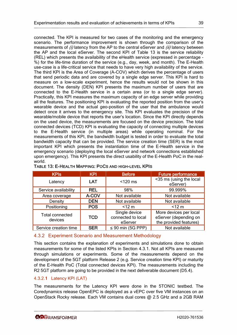
Experimentation results and evaluation of achievements in terms of KPIs 39
H2020-761536
connected. The KPI is measured for two cases of the monitoring and the emergency scenario. The performance improvement is shown through the comparison of the measurements of (i) latency from the AP to the central eServer and (ii) latency between the AP and the local eServer. The second KPI of Table 13 is the service reliability (REL) which presents the availability of the eHealth service (expressed in percentage - %) for the life-time duration of the service (e.g., day, week, and month). The E-Health use-case is a life-critical service that needs to have very high availability of the service. The third KPI is the Area of Coverage (A-COV) which derives the percentage of users that send periodic data and are covered by a single edge server. This KPI is hard to measure on a low-scale experiment, hence the results would not be shown in this document. The density (DEN) KPI presents the maximum number of users that are connected to the E-Health service in a certain area (or to a single edge server). Practically, this KPI measures the maximum capacity of an edge server while providing all the features. The positioning KPI is evaluating the reported position from the user’s wearable device and the actual geo-position of the user that the ambulance would detect once it arrives to the emergency site. This KPI evaluates the precision of the wearable/mobile device that reports the user’s location. Since the KPI directly depends on the used device, the measurements are focused on the device precision. The total connected devices (TCD) KPI is evaluating the capacity of connecting multiple devices to the E-Health service (in multiple areas) while operating nominal. For the measurements of this KPI, the bandwidth budget is tested in order to evaluate the total bandwidth capacity that can be provided. The service creation time (SER) is the most important KPI which presents the instantiation time of the E-Health service in the emergency scenario (deploying the local eServer and network connections established upon emergency). This KPI presents the direct usability of the E-Health PoC in the real-world. TABLE 13: E-HEALTH MAPPING: POCS AND HIGH-LEVEL KPIS
KPIs KPI Before Future performance
Latency LAT <120 ms <35 ms (using the local
eServer)
Service availability REL 98% 99.999%
Area coverage A-COV Not available Not available
Density DEN Not available Not available
Positioning POS <12 m <12 m
Total connected devices
TCD Single device
connected to local eServer
More devices per local eServer (depending on the provided features)
Service creation time SER ≤ 90 min (5G PPP) Not available
4.3.2 Experiment Scenario and Measurement Methodology
This section contains the explanation of experiments and simulations done to obtain
measurements for some of the listed KPIs in Section 4.3.1. Not all KPIs are measured
through simulations or experiments. Some of the measurements depend on the
development of the 5GT platform Release 2 (e.g. Service creation time KPI) or maturity
of the E-Health PoC (Total connected devices KPI). The measurements including the
R2 5GT platform are going to be provided in the next deliverable document (D5.4).
Latency KPI (LAT)
The measurements for the Latency KPI were done in the 5TONIC testbed. The
Coredynamics release OpenEPC is deployed as a vEPC over five VM instances on an
OpenStack Rocky release. Each VM contains dual cores @ 2.5 GHz and a 2GB RAM
Experimentation results and evaluation of achievements in terms of KPIs 40
H2020-761536
memory. A physical device eNB+BBU+RRU is used to connect the UEs to rest of the
vEPC components.
Two sets of measurements were done for measuring the latency. First set is for
measuring the latency between the AP and the central eServer an experiment was run
to emulate the real-world scenario of reaching the central eServer from a UE device. In
this case ping messages sent from the UE to the central eServer are used to measure
the RTT latency. The second set of measurements follows the same methodology of
using ping messages, but in this case from the UE to the local eServer.
Service reliability KPI (REL)
The E-Health PoC is a critical service that demands very high reliability of the service.
For measuring the reliability of the scenario, a data set has been obtained of all critical
emergencies occurring in the area of Madrid, Spain for the duration of year (April 2018-
March 2018) 2. According to the data, a simulation was compiled where every 5 minutes
a user would report an emergency to the central eServer for the duration of 3
consecutive days.
Positioning KPI (POS)
The positioning KPI is independent of the experimental setup scenario and directly
depends of the capabilities of the user’s wearable devices (or mobile devices). The way
it works is that the wearable device reports its GPS position to the central eServer via
the connected mobile device. However some wearable devices don’t contain GPS
chipset due to battery consumption or dimension limitations (size, weight etc.). In that
case the reported GPS location would be the mobile device location.
Total Connected Devices (TCD)
The total connected devices KPI measures the capacity of the local eServer to be able
to serve simultaneously a number of users in emergency states. The measured KPI
provides insight of how many users can be served per local eServer instance. The total
connected devices (TCD) KPI is important measurement to understand the capacity of
a local eServer instance. The TCD is measured through accruing the bandwidth budget
of the local eServer or sending data on the uplink towards the local eServer. From the
total bandwidth budget it is calculated the maximum number of connected devices
while maintaining the QoS per device.
Service creation time KPI (SER)
The service creation time KPI is the most important to measure the real benefit of
having the deployed 5GT platform components for realization of the emergency
scenario in the E-Health PoC. The deployment time of the local eServer closer to the
emergency patient (user) directly impacts on the patient life and the improved response
of the emergency service. For measuring the deployment time, the 5GT platform
Release 2 is needed. At the time of conducting the experiments, the Release 2 is not
available.
4.3.3 Results
In this section the results obtained per each KPI are presented.
2 SAMUR’s emergency statistics for Madrid City from May 2018 to April 2019.
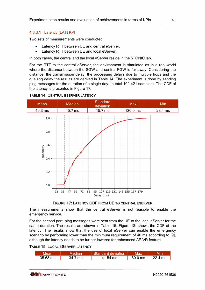
Experimentation results and evaluation of achievements in terms of KPIs 41
H2020-761536
Latency (LAT) KPI
Two sets of measurements were conducted:
• Latency RTT between UE and central eServer.
• Latency RTT between UE and local eServer.
In both cases, the central and the local eServer reside in the 5TONIC lab.
For the RTT to the central eServer, the environment is simulated as in a real-world
where the distance between the SGW and central PGW is far away. Considering the
distance, the transmission delay, the processing delays due to multiple hops and the
queuing delay the results are derived in Table 14. The experiment is done by sending
ping messages for the duration of a single day (in total 102 421 samples). The CDF of
the latency is presented in Figure 17.
TABLE 14: CENTRAL ESERVER LATENCY
Mean Median Standard deviation
Max Min
49.3 ms 45.7 ms 15.7 ms 180.0 ms 23.4 ms
FIGURE 17: LATENCY CDF FROM UE TO CENTRAL ESERVER
The measurements show that the central eServer is not feasible to enable the
emergency service.
For the second part, ping messages were sent from the UE to the local eServer for the
same duration. The results are shown in Table 15. Figure 18: shows the CDF of the
latency. The results show that the use of local eServer can enable the emergency
scenario by performing lower than the minimum requirement of 40 ms according to [9],
although the latency needs to be further lowered for enhcanced AR/VR feature.
TABLE 15: LOCAL ESERVER LATENCY
Mean Median Standard deviation Max Min 35.63 ms 34.7 ms 4.154 ms 80.0 ms 22.4 ms
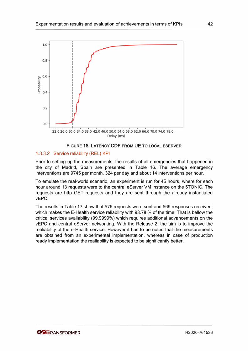
Experimentation results and evaluation of achievements in terms of KPIs 42
H2020-761536
FIGURE 18: LATENCY CDF FROM UE TO LOCAL ESERVER
Service reliability (REL) KPI
Prior to setting up the measurements, the results of all emergencies that happened in
the city of Madrid, Spain are presented in Table 16. The average emergency
interventions are 9745 per month, 324 per day and about 14 interventions per hour.
To emulate the real-world scenario, an experiment is run for 45 hours, where for each
hour around 13 requests were to the central eServer VM instance on the 5TONIC. The
requests are http GET requests and they are sent through the already instantiated
vEPC.
The results in Table 17 show that 576 requests were sent and 569 responses received,
which makes the E-Health service reliability with 98.78 % of the time. That is bellow the
critical services availability (99.9999%) which requires additional advancements on the
vEPC and central eServer networking. With the Release 2, the aim is to improve the
realiability of the e-Health service. However it has to be noted that the measurements
are obtained from an experimental implementation, whereas in case of production
ready implementation the realiability is expected to be significantly better.
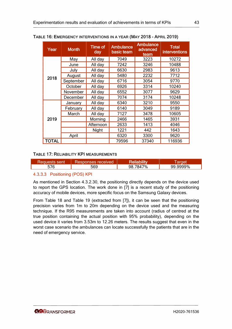
Experimentation results and evaluation of achievements in terms of KPIs 43
H2020-761536
TABLE 16: EMERGENCY INTERVENTIONS IN A YEAR (MAY 2018 - APRIL 2019)
Year Month Time of
day Ambulance basic team
Ambulance advanced
team
Total interventions
2018
May All day 7049 3223 10272
June All day 7242 3246 10488
July All day 6630 2983 9613
August All day 5480 2232 7712
September All day 6716 3054 9770
October All day 6926 3314 10240
November All day 6552 3077 9629
December All day 7074 3174 10248
2019
January All day 6340 3210 9550
February All day 6140 3049 9189
March All day 7127 3478 10605
Morning 2466 1465 3931
Afternoon 2633 1413 4046
Night 1221 442 1643
April 6320 3300 9620
TOTAL 79596 37340 116936
TABLE 17: RELIABILITY KPI MEASUREMENTS
Requests sent Responses received Reliability Target 576 569 98.7847% 99.9999%
Positioning (POS) KPI
As mentioned in Section 4.3.2.30, the positioning directly depends on the device used
to report the GPS location. The work done in [7] is a recent study of the positioning
accuracy of mobile devices, more specific focus on the Samsung Galaxy devices.
From Table 18 and Table 19 (extracted from [7]), it can be seen that the positioning
precision varies from 1m to 20m depending on the device used and the measuring
technique. If the R95 measurements are taken into account (radius of centred at the
true position containing the actual position with 95% probability), depending on the
used device it varies from 3.53m to 12.26 meters. The results suggest that even in the
worst case scenario the ambulances can locate successfully the patients that are in the
need of emergency service.
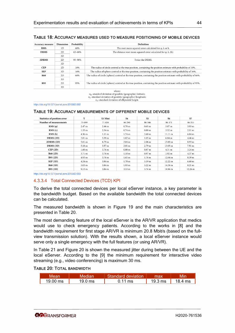
Experimentation results and evaluation of achievements in terms of KPIs 44
H2020-761536
TABLE 18: ACCURACY MEASURES USED TO MEASURE POSITIONING OF MOBILE DEVICES
TABLE 19: ACCURACY MEASUREMENTS OF DIFFERENT MOBILE DEVICES
Total Connected Devices (TCD) KPI
To derive the total connected devices per local eServer instance, a key parameter is
the bandwidth budget. Based on the available bandwidth the total connected devices
can be calculated.
The measured bandwidth is shown in Figure 19 and the main characteristics are
presented in Table 20.
The most demanding feature of the local eServer is the AR/VR application that medics
would use to check emergency patients. According to the works in [8] and the
bandwidth requirement for first stage AR/VR is minimum 20.8 Mbit/s (based on the full-
view transmission solution). With the results shown, a local eServer instance would
serve only a single emergency with the full features (or using AR/VR).
In Table 21 and Figure 20 is shown the measured jitter during between the UE and the
local eServer. According to the [9] the minimum requirement for interactive video
streaming (e.g., video conferencing) is maximum 30 ms.
TABLE 20: TOTAL BANDWIDTH
Mean Median Standard deviation max Min 19.00 ms 19.0 ms 0.11 ms 19.3 ms 18.4 ms
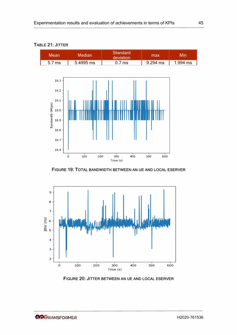
Experimentation results and evaluation of achievements in terms of KPIs 45
H2020-761536
TABLE 21: JITTER
Mean Median Standard deviation
max Min
5.7 ms 5.4995 ms 0.7 ms 9.294 ms 1.994 ms
FIGURE 19: TOTAL BANDWIDTH BETWEEN AN UE AND LOCAL ESERVER
FIGURE 20: JITTER BETWEEN AN UE AND LOCAL ESERVER
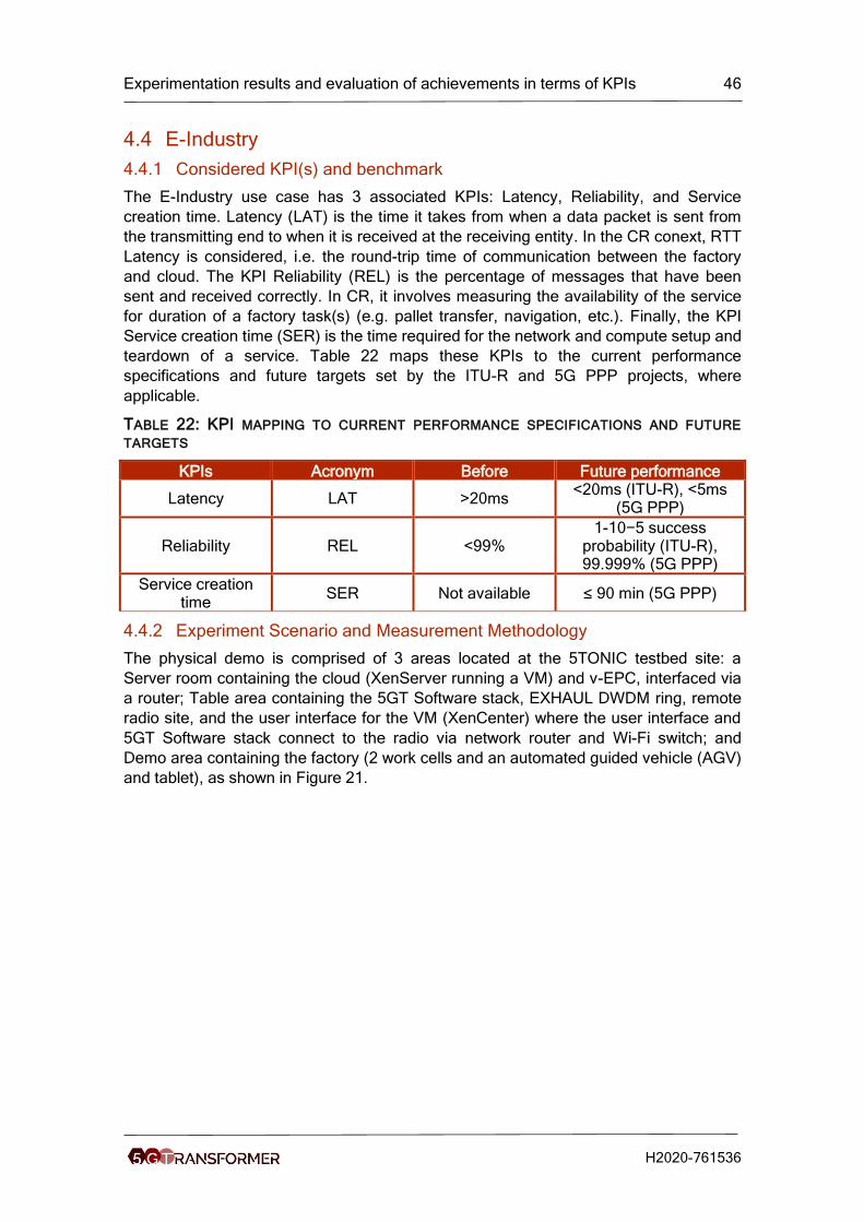
Experimentation results and evaluation of achievements in terms of KPIs 46
H2020-761536
4.4 E-Industry
4.4.1 Considered KPI(s) and benchmark
The E-Industry use case has 3 associated KPIs: Latency, Reliability, and Service
creation time. Latency (LAT) is the time it takes from when a data packet is sent from
the transmitting end to when it is received at the receiving entity. In the CR conext, RTT
Latency is considered, i.e. the round-trip time of communication between the factory
and cloud. The KPI Reliability (REL) is the percentage of messages that have been
sent and received correctly. In CR, it involves measuring the availability of the service
for duration of a factory task(s) (e.g. pallet transfer, navigation, etc.). Finally, the KPI
Service creation time (SER) is the time required for the network and compute setup and
teardown of a service. Table 22 maps these KPIs to the current performance
specifications and future targets set by the ITU-R and 5G PPP projects, where
applicable.
TABLE 22: KPI MAPPING TO CURRENT PERFORMANCE SPECIFICATIONS AND FUTURE
TARGETS
KPIs Acronym Before Future performance
Latency LAT >20ms <20ms (ITU-R), <5ms
(5G PPP)
Reliability REL <99% 1-10−5 success
probability (ITU-R), 99.999% (5G PPP)
Service creation time
SER Not available ≤ 90 min (5G PPP)
4.4.2 Experiment Scenario and Measurement Methodology
The physical demo is comprised of 3 areas located at the 5TONIC testbed site: a
Server room containing the cloud (XenServer running a VM) and v-EPC, interfaced via
a router; Table area containing the 5GT Software stack, EXHAUL DWDM ring, remote
radio site, and the user interface for the VM (XenCenter) where the user interface and
5GT Software stack connect to the radio via network router and Wi-Fi switch; and
Demo area containing the factory (2 work cells and an automated guided vehicle (AGV)
and tablet), as shown in Figure 21.
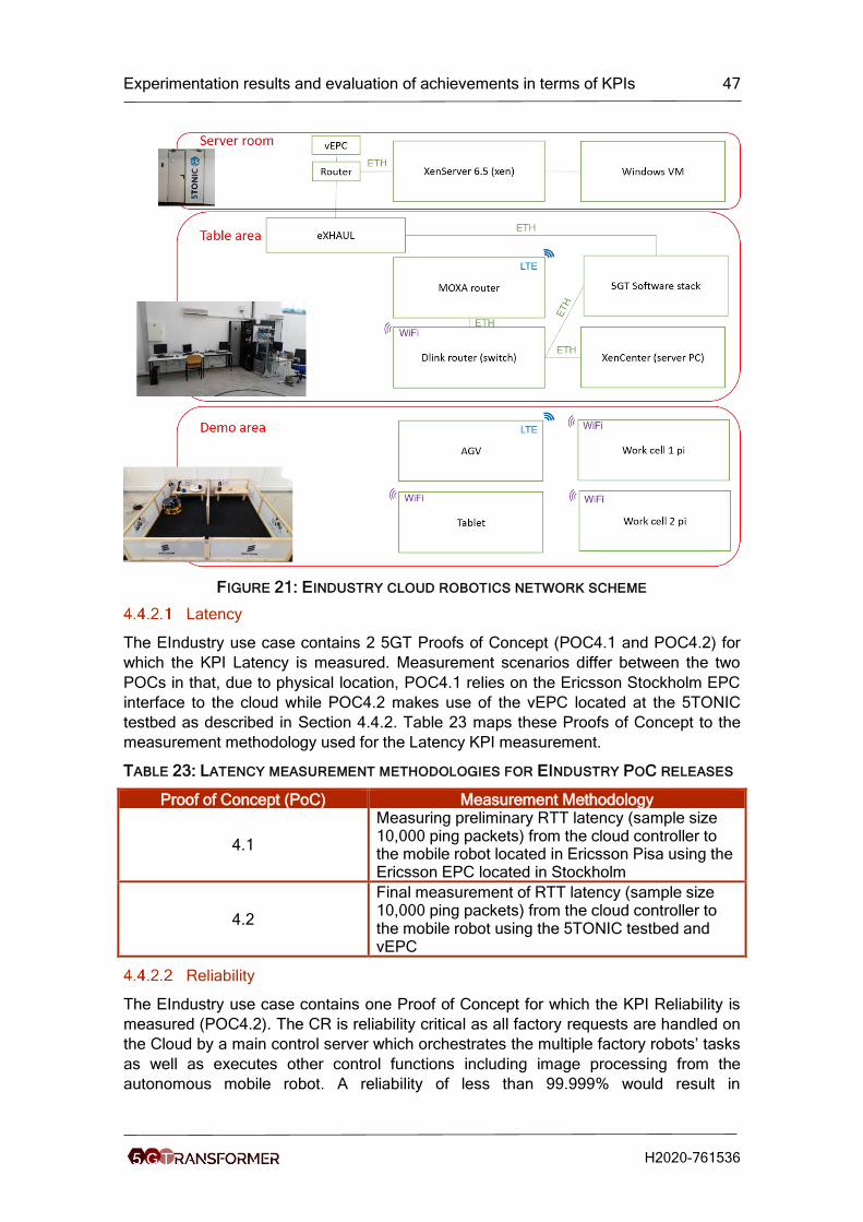
Experimentation results and evaluation of achievements in terms of KPIs 47
H2020-761536
FIGURE 21: EINDUSTRY CLOUD ROBOTICS NETWORK SCHEME
Latency
The EIndustry use case contains 2 5GT Proofs of Concept (POC4.1 and POC4.2) for
which the KPI Latency is measured. Measurement scenarios differ between the two
POCs in that, due to physical location, POC4.1 relies on the Ericsson Stockholm EPC
interface to the cloud while POC4.2 makes use of the vEPC located at the 5TONIC
testbed as described in Section 4.4.2. Table 23 maps these Proofs of Concept to the
measurement methodology used for the Latency KPI measurement.
TABLE 23: LATENCY MEASUREMENT METHODOLOGIES FOR EINDUSTRY POC RELEASES
Proof of Concept (PoC) Measurement Methodology
4.1
Measuring preliminary RTT latency (sample size 10,000 ping packets) from the cloud controller to the mobile robot located in Ericsson Pisa using the Ericsson EPC located in Stockholm
4.2
Final measurement of RTT latency (sample size 10,000 ping packets) from the cloud controller to the mobile robot using the 5TONIC testbed and vEPC
Reliability
The EIndustry use case contains one Proof of Concept for which the KPI Reliability is
measured (POC4.2). The CR is reliability critical as all factory requests are handled on
the Cloud by a main control server which orchestrates the multiple factory robots’ tasks
as well as executes other control functions including image processing from the
autonomous mobile robot. A reliability of less than 99.999% would result in
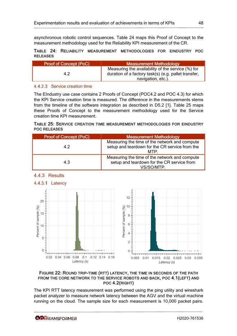
Experimentation results and evaluation of achievements in terms of KPIs 48
H2020-761536
asynchronous robotic control sequences. Table 24 maps this Proof of Concept to the
measurement methodology used for the Reliability KPI measurement of the CR.
TABLE 24: RELIABILITY MEASUREMENT METHODOLOGIES FOR EINDUSTRY POC
RELEASES
Proof of Concept (PoC) Measurement Methodology
4.2 Measuring the availability of the service (%) for duration of a factory task(s) (e.g. pallet transfer,
navigation, etc.).
Service creation time
The EIndustry use case contains 2 Proofs of Concept (POC4.2 and POC 4.3) for which
the KPI Service creation time is measured. The difference in the measurements stems
from the timeline of the software integration as described in D5.2 [1]. Table 25 maps
these Proofs of Concept to the measurement methodology used for the Service
creation time KPI measurement.
TABLE 25: SERVICE CREATION TIME MEASUREMENT METHODOLOGIES FOR EINDUSTRY
POC RELEASES
Proof of Concept (PoC) Measurement Methodology
4.2 Measuring the time of the network and compute setup and teardown for the CR service from the
MTP.
4.3 Measuring the time of the network and compute
setup and teardown for the CR service from VS/SO/MTP.
4.4.3 Results
Latency
FIGURE 22: ROUND TRIP-TIME (RTT) LATENCY, THE TIME IN SECONDS OF THE PATH
FROM THE CORE NETWORK TO THE SERVICE ROBOTS AND BACK, POC 4.1(LEFT) AND
POC 4.2(RIGHT)
The KPI RTT latency measurement was performed using the ping utility and wireshark
packet analyzer to measure network latency between the AGV and the virtual machine
running on the cloud. The sample size for each measurement is 10,000 packet pairs.
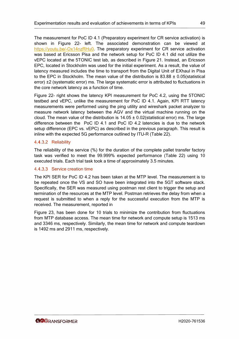
Experimentation results and evaluation of achievements in terms of KPIs 49
H2020-761536
The measurement for PoC ID 4.1 (Preparatory experiment for CR service activation) is
shown in Figure 22- left. The associated demonstration can be viewed at
https://youtu.be/-Ox14nzRHu0. The preparatory experiment for CR service activation
was based at Ericsson Pisa and the network setup for PoC ID 4.1 did not utilize the
vEPC located at the 5TONIC test lab, as described in Figure 21. Instead, an Ericsson
EPC, located in Stockholm was used for the initial experiment. As a result, the value of
latency measured includes the time to transport from the Digital Unit of EXhaul in Pisa
to the EPC in Stockholm. The mean value of the distribution is 83.88 ± 0.05(statistical
error) ±2 (systematic error) ms. The large systematic error is attributed to fluctuations in
the core network latency as a function of time.
Figure 22- right shows the latency KPI measurement for PoC 4.2, using the 5TONIC
testbed and vEPC, unlike the measurement for PoC ID 4.1. Again, KPI RTT latency
measurements were performed using the ping utility and wireshark packet analyzer to
measure network latency between the AGV and the virtual machine running on the
cloud. The mean value of the distribution is 14.05 ± 0.02(statistical error) ms. The large
difference between the PoC ID 4.1 and PoC ID 4.2 latencies is due to the network
setup difference (EPC vs. vEPC) as described in the previous paragraph. This result is
inline with the expected 5G performance outlined by ITU-R (Table 22).
Reliability
The reliability of the service (%) for the duration of the complete pallet transfer factory
task was verified to meet the 99.999% expected performance (Table 22) using 10
executed trials. Each trial task took a time of approximately 3.5 minutes.
Service creation time
The KPI SER for PoC ID 4.2 has been taken at the MTP level. The measurement is to
be repeated once the VS and SO have been integrated into the 5GT software stack.
Specifically, the SER was measured using postman rest client to trigger the setup and
termination of the resources at the MTP level. Postman retrieves the delay from when a
request is submitted to when a reply for the successful execution from the MTP is
received. The measurement, reported in
Figure 23, has been done for 10 trials to minimize the contribution from fluctuations
from MTP database access. The mean time for network and compute setup is 1513 ms
and 3346 ms, respectively. Similarly, the mean time for network and compute teardown
is 1492 ms and 2911 ms, respectively.
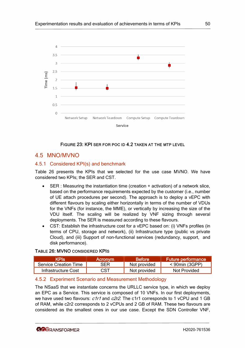
Experimentation results and evaluation of achievements in terms of KPIs 50
H2020-761536
FIGURE 23: KPI SER FOR POC ID 4.2 TAKEN AT THE MTP LEVEL
4.5 MNO/MVNO
4.5.1 Considered KPI(s) and benchmark
Table 26 presents the KPIs that we selected for the use case MVNO. We have
considered two KPIs; the SER and CST.
• SER : Measuring the instantiation time (creation + activation) of a network slice,
based on the performance requirements expected by the customer (i.e., number
of UE attach procedures per second). The approach is to deploy a vEPC with
different flavours by scaling either horizontally in terms of the number of VDUs
for the VNFs (for instance, the MME), or vertically by increasing the size of the
VDU itself. The scaling will be realized by VNF sizing through several
deployments. The SER is measured according to these flavours.
• CST: Establish the infrastructure cost for a vEPC based on: (i) VNFs profiles (in
terms of CPU, storage and network), (ii) Infrastructure type (public vs private
Cloud), and (iii) Support of non-functional services (redundancy, support, and
disk performance).
TABLE 26: MVNO CONSIDERED KPIS
KPIs Acronym Before Future performance Service Creation Time SER Not provided < 90min (3GPP)
Infrastructure Cost CST Not provided Not Provided
4.5.2 Experiment Scenario and Measurement Methodology
The NSaaS that we instantiate concerns the URLLC service type, in which we deploy
an EPC as a Service. This service is composed of 10 VNFs. In our first deployments,
we have used two flavours: c1r1 and c2r2. The c1r1 corresponds to 1 vCPU and 1 GB
of RAM, while c2r2 corresponds to 2 vCPUs and 2 GB of RAM. These two flavours are
considered as the smallest ones in our use case. Except the SDN Controller VNF,
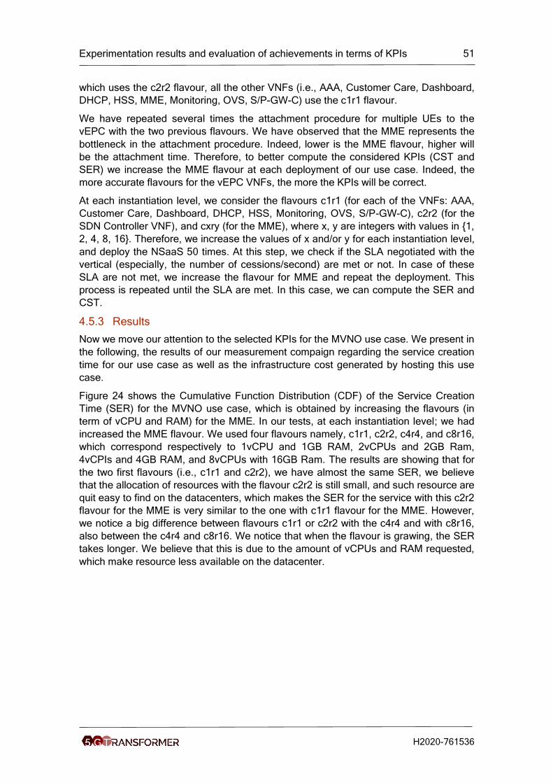
Experimentation results and evaluation of achievements in terms of KPIs 51
H2020-761536
which uses the c2r2 flavour, all the other VNFs (i.e., AAA, Customer Care, Dashboard,
DHCP, HSS, MME, Monitoring, OVS, S/P-GW-C) use the c1r1 flavour.
We have repeated several times the attachment procedure for multiple UEs to the
vEPC with the two previous flavours. We have observed that the MME represents the
bottleneck in the attachment procedure. Indeed, lower is the MME flavour, higher will
be the attachment time. Therefore, to better compute the considered KPIs (CST and
SER) we increase the MME flavour at each deployment of our use case. Indeed, the
more accurate flavours for the vEPC VNFs, the more the KPIs will be correct.
At each instantiation level, we consider the flavours c1r1 (for each of the VNFs: AAA,
Customer Care, Dashboard, DHCP, HSS, Monitoring, OVS, S/P-GW-C), c2r2 (for the
SDN Controller VNF), and cxry (for the MME), where x, y are integers with values in {1,
2, 4, 8, 16}. Therefore, we increase the values of x and/or y for each instantiation level,
and deploy the NSaaS 50 times. At this step, we check if the SLA negotiated with the
vertical (especially, the number of cessions/second) are met or not. In case of these
SLA are not met, we increase the flavour for MME and repeat the deployment. This
process is repeated until the SLA are met. In this case, we can compute the SER and
CST.
4.5.3 Results
Now we move our attention to the selected KPIs for the MVNO use case. We present in
the following, the results of our measurement compaign regarding the service creation
time for our use case as well as the infrastructure cost generated by hosting this use
case.
Figure 24 shows the Cumulative Function Distribution (CDF) of the Service Creation
Time (SER) for the MVNO use case, which is obtained by increasing the flavours (in
term of vCPU and RAM) for the MME. In our tests, at each instantiation level; we had
increased the MME flavour. We used four flavours namely, c1r1, c2r2, c4r4, and c8r16,
which correspond respectively to 1vCPU and 1GB RAM, 2vCPUs and 2GB Ram,
4vCPIs and 4GB RAM, and 8vCPUs with 16GB Ram. The results are showing that for
the two first flavours (i.e., c1r1 and c2r2), we have almost the same SER, we believe
that the allocation of resources with the flavour c2r2 is still small, and such resource are
quit easy to find on the datacenters, which makes the SER for the service with this c2r2
flavour for the MME is very similar to the one with c1r1 flavour for the MME. However,
we notice a big difference between flavours c1r1 or c2r2 with the c4r4 and with c8r16,
also between the c4r4 and c8r16. We notice that when the flavour is grawing, the SER
takes longer. We believe that this is due to the amount of vCPUs and RAM requested,
which make resource less available on the datacenter.
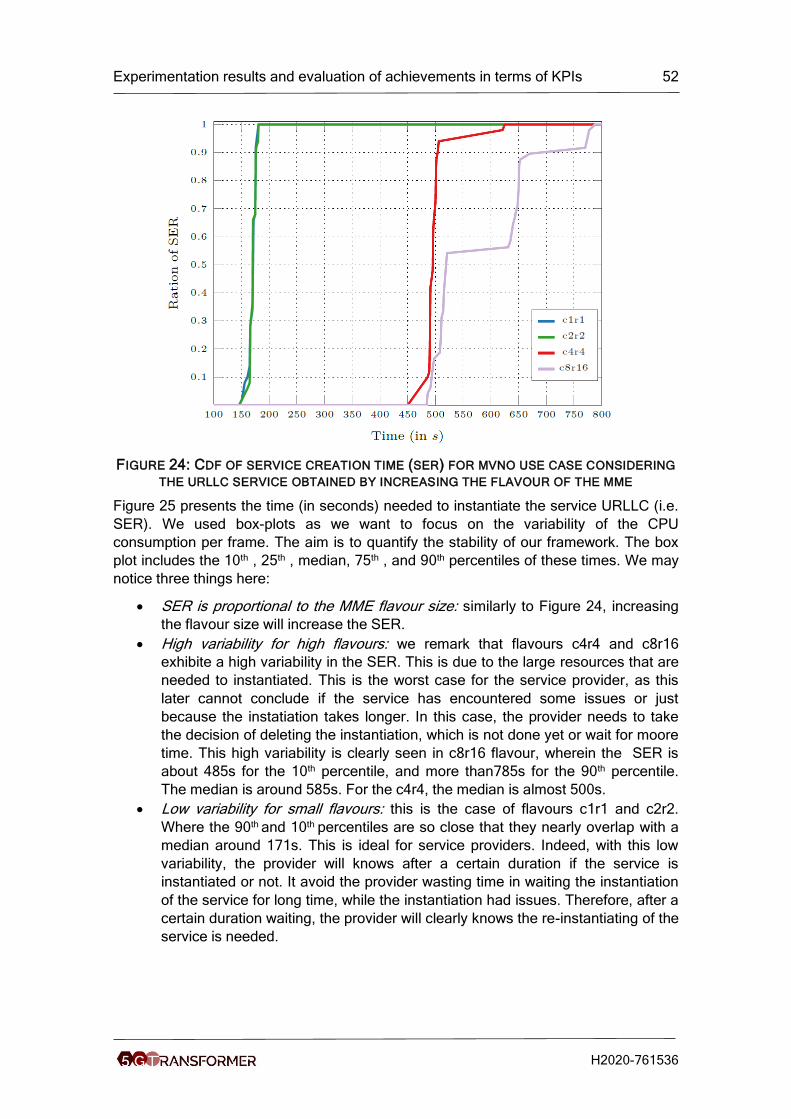
Experimentation results and evaluation of achievements in terms of KPIs 52
H2020-761536
FIGURE 24: CDF OF SERVICE CREATION TIME (SER) FOR MVNO USE CASE CONSIDERING
THE URLLC SERVICE OBTAINED BY INCREASING THE FLAVOUR OF THE MME
Figure 25 presents the time (in seconds) needed to instantiate the service URLLC (i.e.
SER). We used box-plots as we want to focus on the variability of the CPU
consumption per frame. The aim is to quantify the stability of our framework. The box
plot includes the 10th , 25th , median, 75th , and 90th percentiles of these times. We may
notice three things here:
• SER is proportional to the MME flavour size: similarly to Figure 24, increasing
the flavour size will increase the SER.
• High variability for high flavours: we remark that flavours c4r4 and c8r16
exhibite a high variability in the SER. This is due to the large resources that are
needed to instantiated. This is the worst case for the service provider, as this
later cannot conclude if the service has encountered some issues or just
because the instatiation takes longer. In this case, the provider needs to take
the decision of deleting the instantiation, which is not done yet or wait for moore
time. This high variability is clearly seen in c8r16 flavour, wherein the SER is
about 485s for the 10th percentile, and more than785s for the 90th percentile.
The median is around 585s. For the c4r4, the median is almost 500s.
• Low variability for small flavours: this is the case of flavours c1r1 and c2r2.
Where the 90th and 10th percentiles are so close that they nearly overlap with a
median around 171s. This is ideal for service providers. Indeed, with this low
variability, the provider will knows after a certain duration if the service is
instantiated or not. It avoid the provider wasting time in waiting the instantiation
of the service for long time, while the instantiation had issues. Therefore, after a
certain duration waiting, the provider will clearly knows the re-instantiating of the
service is needed.
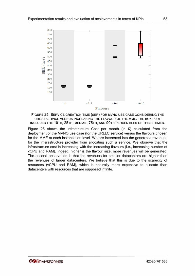
Experimentation results and evaluation of achievements in terms of KPIs 53
H2020-761536
FIGURE 25: SERVICE CREATION TIME (SER) FOR MVNO USE CASE CONSIDERING THE
URLLC SERVICE VERSUS INCREASING THE FLAVOUR OF THE MME. THE BOX PLOT
INCLUDES THE 10TH, 25TH, MEDIAN, 75TH, AND 90TH PERCENTILES OF THESE TIMES.
Figure 26 shows the infrastructure Cost per month (in €) calculated from the
deployment of the MVNO use case (for the URLLC service) versus the flavours chosen
for the MME at each instantiation level. We are interested into the generated revenues
for the infsrastructure provider from allocating such a service. We observe that the
infrastructure cost in increasing with the increasing flavours (i.e., increasing number of
vCPU and RAM). Indeed, higher is the flavour size, more revenues will be generated.
The second observation is that the revenues for smaller datacenters are higher than
the revenues of larger datacenters. We believe that this is due to the scarecity of
resources (vCPU and RAM), which is naturally more expensive to allocate than
datacenters with resources that are supposed infinite.
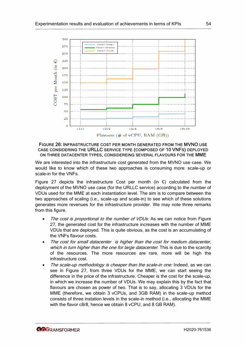
Experimentation results and evaluation of achievements in terms of KPIs 54
H2020-761536
FIGURE 26: INFRASTRUCTURE COST PER MONTH GENERATED FROM THE MVNO USE
CASE CONSIDERING THE URLLC SERVICE TYPE (COMPOSED OF 10 VNFS) DEPLOYED
ON THREE DATACENTER TYPES, CONSIDEREING SEVERAL FLAVOURS FOR THE MME
We are interested into the infrastructure cost generated from the MVNO use case. We
would like to know which of these two approaches is consuming more: scale-up or
scale-in for the VNFs.
Figure 27 depicts the infrastructure Cost per month (in €) calculated from the
deployment of the MVNO use case (for the URLLC service) according to the number of
VDUs used for the MME at each instantiation level. The aim is to compare between the
two approaches of scaling (i.e., scale-up and scale-in) to see which of these solutions
generates more revenues for the infrastructure provider. We may note three remarks
from this figure.
• The cost is proportional to the number of VDUs: As we can notice from Figure
27, the generated cost for the infrastructure increases with the number of MME
VDUs that are deployed. This is quite obvious, as the cost is an accumulating of
the VNFs flavour costs.
• The cost for small datacenter is higher than the cost for medium datacenter,
which in turn higher than the one for large datacenter: This is due to the scarcity
of the resources. The more resources are rare, more will be high the
infrastructure cost.
• The scale-up methodology is cheaper than the scale-in one: Indeed, as we can
see in Figure 27, from three VDUs for the MME, we can start seeing the
difference in the price of the infrastructure. Cheaper is the cost for the scale-up,
in which we increase the number of VDUs. We may explain this by the fact that
flavours are chosen as power of two. That is to say, allocating 3 VDUs for the
MME (therefore, we obtain 3 vCPUs, and 3GB RAM) in the scale-up method
consists of three instation levels in the scale-in method (i.e., allocating the MME
with the flavor c8r8, hence we obtain 8 vCPU, and 8 GB RAM).
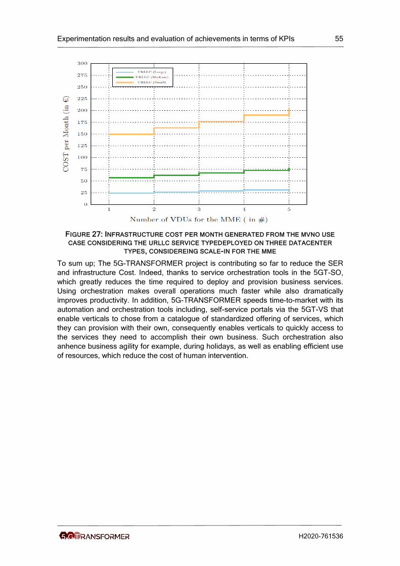
Experimentation results and evaluation of achievements in terms of KPIs 55
H2020-761536
FIGURE 27: INFRASTRUCTURE COST PER MONTH GENERATED FROM THE MVNO USE
CASE CONSIDERING THE URLLC SERVICE TYPEDEPLOYED ON THREE DATACENTER
TYPES, CONSIDEREING SCALE-IN FOR THE MME
To sum up; The 5G-TRANSFORMER project is contributing so far to reduce the SER
and infrastructure Cost. Indeed, thanks to service orchestration tools in the 5GT-SO,
which greatly reduces the time required to deploy and provision business services.
Using orchestration makes overall operations much faster while also dramatically
improves productivity. In addition, 5G-TRANSFORMER speeds time-to-market with its
automation and orchestration tools including, self-service portals via the 5GT-VS that
enable verticals to chose from a catalogue of standardized offering of services, which
they can provision with their own, consequently enables verticals to quickly access to
the services they need to accomplish their own business. Such orchestration also
anhence business agility for example, during holidays, as well as enabling efficient use
of resources, which reduce the cost of human intervention.
Experimentation results and evaluation of achievements in terms of KPIs 56
H2020-761536
5 Additional evaluation This section reports some additional performance evaluation related to 5GT KPIs that
has been conducted outside of the official PoCs. Such evaluation complements the one
performed in the PoCs with more focus on the utilized technology and with
applications/verticals that are different from the ones considered in the PoCs.
In section 5.1 the evaluation of the jitter (i.e., delay variation) introduced by different
virtualisation technologies (e.g., docker container and kvm) are performend for a
proprietary application and with cyclictest. Such jitter can impact the LAT KPI becasue
part of the latency budget has to be used to compensate for the processing jitter.
In section 5.2 it is reported the evaluation of the time requested by the 5GT platform to
setup a 5G network slice (i.e., the the network reosurces to connect a mobile phone to
the Internet). Such time contributes to the SER KPI because it is a measure of the time
elapsing between the mobile network slice request and the successful slice delivery.
In section 5.3 additional evaluation of specific algorithms utilized by the 5GT-MTP is
provided. Such evaluation is performed through simulations to highlight their
contribution to the overall 5G-TRANSFORMER objectives and 5G-PPP KPIs. In
particular, a logical link placement algorithm, a VNF placement algorithm minimizing
the power consumption of the NFVI-PoPs managed by the 5G-TRANSFORMER
platform, a rigorous analytical framework, called FLuidRAN, for the optimized
configuration of virtual RAN (vRAN) networks, an algorithm for dynamic de/activation of
VMs based on the requested elaboration are detailed and evaluated. In addition, their
contribution to the 5G-PPP performance KPIs is highlighted.
5.1 Real-time computation in virtualized environments
E2E latencies of vertical services are impacted by various factors such as the latency at
the air interface, latencies in the transport network as well as processing latencies
themselves. Services with very stringent requirements on E2E latencies will have
correspondingly stringent requirements on the processing latencies of the applications.
Many of these applications can be considered as real-time applications, e.g. control of
AGVs or baseband processing of virtualized base stations.
Virtualization platforms are often built on top of operating systems and COTS hardware,
which have not been developed for real-time usage. Two typical virtualization
approaches are virtual machines on top of a hypervisor and a tighter integration with
the host operating system using containers. The host and guest operating system as
well as the virtualization approach have an impact on processing jitter, i.e. the variation
on the duration of computations.
In the following we present measurements of processing jitter without virtualization
(bare-metal), container-based virtualization (docker), hypervisor-based virtualization
(kvm), and containers within virtual machines. The measurements have been done
both for a non-optimized Linux version (Ubuntu 16.0.4) and with configurations
improving the real-time behaviour.
5.1.1 Considered KPI(s) and benchmark
For real-time computation it is important to meet processing deadlines. Therefore, one
has to know how much processing time jitter and how precisely timer interrupts are
Experimentation results and evaluation of achievements in terms of KPIs 57
H2020-761536
met. It is not sufficient to determine the average processing jitter; one has to know as
well to which degree the processing jitter is deviating from the average value.
As benchmark we take execution of applications on a bare-metal server, i.e. without
any virtualization technology, expecting that the processing jitter will be larger for the
different virtualization approaches. Container-based and hypervisor-based virtualization
are the most commonly used virtualization approaches in the field. Executing
containers inside a VM is a common approach to increase isolation among tenants, by
using separate virtual machines per tenant, but keeping the fast deployment of
containers inside each VM. I.e. there is one virtual machine per tenant on a host, with
multiple containers executed in each VM.
5.1.2 Experiment/Simulation Scenario and Measurement Methodology
The tests have been performed on server blades (srv11, srv12, srv14) of three different
vendors. All blades use Intel® Xeon® processors of different version and chipsets (see
Appendix A for a more detailed HW summary). CPU frequency has been fixed on all
servers to 1700MHz with hyper-threading turned off.
For srv11 there was a need to disable system management interrupts (SMI), allowing
for processing jitter below 100s. [12] provides tests to verify whether jitter caused by
SMIs are within a tolerable limit (currently defined as 150s). For further details on HP®
SMI server configuration, please see [11].
The tests have been performed on standard Ubuntu 16.04.6 LTS, with same settings
on all servers. The kernel version used was 4.4.0-143.
For the non-optimized Linux configuration just the intel_pstate kernel boot parameter
has been disabled. This allows to set manual CPU frequency scaling. The CPU
frequency on all serves was set to 1700MHz to allow comparison of the measured
times among the servers. Fixing the CPU frequency is actually beneficial to processing
jitter as there is no variation in processing speed.
The kernel boot parameters in Table 27 have been set additionally for the optimized
Linux configuration, for further detail see [13]. All of these parameters aim to keep Linux
specific tasks away from cores used for the applications.
TABLE 27: OPTIMIZED LINUX CONFIGURATION BOOT PARAMETERS
Boot Parameter Explanation
acpi_irq_nobalance: true avoid IRQs on these cores
noirqbalance: true avoid IRQs on these cores
isolcpus: 4,5 don’t use these cores for any non-explicit use case
mce: ignore_ce disable features for corrected errors
nohz_full: 4,5 allow for “tickles” kernel on these cores
rcu_nocbs: 4,5 no kernel callbacks on these cores
nosoftlockup: true avoid starting kthreads detecting sw lockups
Experimentation results and evaluation of achievements in terms of KPIs 58
H2020-761536
Additional dynamic settings ensure the measurement applications are executed on
dedicated cores, which are not used for Linux specific tasks. These settings are
described in Table 28.
TABLE 28: OPTIMIZED LINUX CONFIGURATION DYNAMIC SETTINGS
Linux Setting Explanation
/proc/sys/kernel/sched_rt_runtime_us = -1
setup realtime scheduler
/proc/sys/kernel/watchdog = 0
disable lockup detection
<via taskset assignment>
assign RCU threads to core 0 assign block device writeback threads to core 0
echo 1 > /sys/bus/workqueue/devices/writeback/cpumask
disable IRQ for selected CPU Core
“/proc/irq/default_smp_affinity” and “/proc/irq/<irq>/smp_affinity” settings
make sure IRQs are rerouted from cores
switch core offline and online again
move existing IRQ handling to different core
nosoftlockup: true avoid starting kthreads detecting software lockups
The measurements are executed on a dedicated core.
The proprietary test measures the time between two consecutive rdtscp operations
(read the Timestamp Counter (TSC) value).
cyclictest [14] measures how accurately a thread is woken up after a timer. It is a part of
the Ubuntu rt-tests package. It has been called with cyclictest -a 4 -H 30 -i
100 -l <iterations> -m -n -p 99 -q -t 1.
5.1.3 Results
Both the proprietary measurement and cyclictest provide the average and the
maximum processing jitter and how often specific values occurred. All measurements
show a similar pattern, which makes it difficult to present a meaningful diagram with
cumulative distribution functions (CDF). As an example, a measurement with cyclictest
of 5 minutes duration contains 3x10^6 individual measurements. As can be seen from
table there are almost no occurrences of values with 1 or 2 s processing jitter. Almost
all individual measurements have 3 or 4 s processing jitter, followed by a tail of values
with just a few individual measurements per value.
Experimentation results and evaluation of achievements in terms of KPIs 59
H2020-761536
TABLE 29: TYPICAL DISTRIBUTION OF MEASURED VALUES
Processing jitter Number of values
1s 0
2s 6
3s 2011864
4s 941386
5s 38146
6s 538
7s 164
8s 153
9s 132
10s 159
… …
The corresponding CDF would start with an almost flat part, followed by a huge and
steep increase, followed again by an almost flat part. A diagram of such a CDF does
not provide a useful visualization. Therefore, we are showing four specific values of
these measurements: the average, 99,999-percentile, 99,9999-percentile, and
maximum values. We derived these values from each measurement. The 99,999-
percentile indicates the processing jitter, which is larger than 99,999% of the individual
measurements and smaller than the remaining 0,001% of the individual measurements.
I.e. 1 out of 10000 individual measurements are exceeding this value. The 99,9999-
percentile is defined similarly.
To increase statistical significance, we repeated each measurement several times.
Each measurement of 5 minutes and 1 hour duration was repeated 12 times. Each
measurement of 1 day duration was repeated 3 times. Then we combined the four
values mentioned above for each of these measurement campaigns. The average,
99,999-percentile and 99,9999-percentiles of a measurement campaign are the
averages of the values of each measurement. Whereas for the maximum processing
jitter of the campaign we have taken the maximum of the maximum values of the
measurements.
As a first result we present the measured results for the optimized Linux configuration,
see Figure 28. The average processing jitter of all virtualization approaches is below
0.1 s, with some differences among the different servers. The 99.999-percentile of
bare-metal and container-based virtualization are almost the same as the average
values, i.e. almost all values are close to the average. For hypervisor-based
virtualization the 99,999-percentile increases to values up to 10 s. The 99.9999-
percentile values are between 1 and 10 s for bare-metal and container-based
virtualization, they are above 10% for hypervisor-based virtualization. This indicates,
that the average processing jitter among the virtualization approaches is similar, but the
tail of values exceeding the average is significantly larger for the hypervisor-based
approaches.
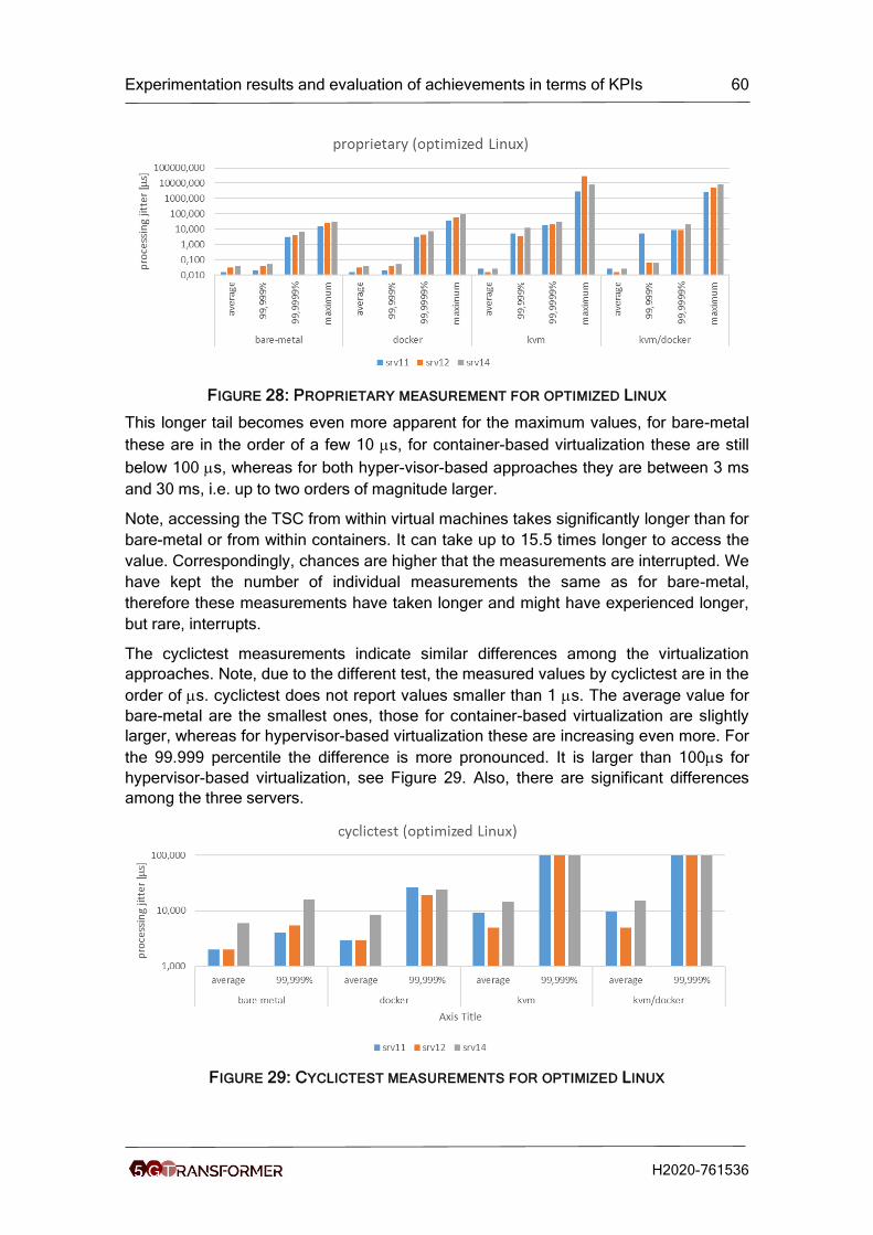
Experimentation results and evaluation of achievements in terms of KPIs 60
H2020-761536
FIGURE 28: PROPRIETARY MEASUREMENT FOR OPTIMIZED LINUX
This longer tail becomes even more apparent for the maximum values, for bare-metal
these are in the order of a few 10 s, for container-based virtualization these are still
below 100 s, whereas for both hyper-visor-based approaches they are between 3 ms
and 30 ms, i.e. up to two orders of magnitude larger.
Note, accessing the TSC from within virtual machines takes significantly longer than for
bare-metal or from within containers. It can take up to 15.5 times longer to access the
value. Correspondingly, chances are higher that the measurements are interrupted. We
have kept the number of individual measurements the same as for bare-metal,
therefore these measurements have taken longer and might have experienced longer,
but rare, interrupts.
The cyclictest measurements indicate similar differences among the virtualization
approaches. Note, due to the different test, the measured values by cyclictest are in the
order of s. cyclictest does not report values smaller than 1 s. The average value for
bare-metal are the smallest ones, those for container-based virtualization are slightly
larger, whereas for hypervisor-based virtualization these are increasing even more. For
the 99.999 percentile the difference is more pronounced. It is larger than 100s for
hypervisor-based virtualization, see Figure 29. Also, there are significant differences
among the three servers.
FIGURE 29: CYCLICTEST MEASUREMENTS FOR OPTIMIZED LINUX
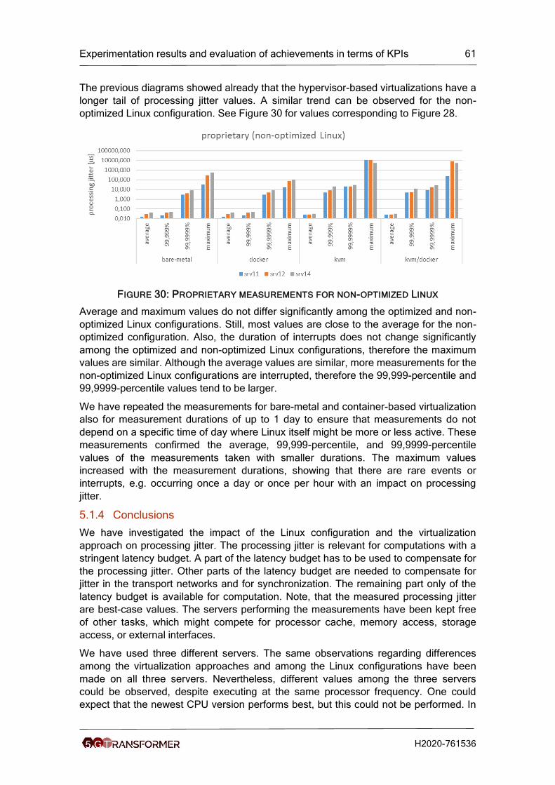
Experimentation results and evaluation of achievements in terms of KPIs 61
H2020-761536
The previous diagrams showed already that the hypervisor-based virtualizations have a
longer tail of processing jitter values. A similar trend can be observed for the non-
optimized Linux configuration. See Figure 30 for values corresponding to Figure 28.
FIGURE 30: PROPRIETARY MEASUREMENTS FOR NON-OPTIMIZED LINUX
Average and maximum values do not differ significantly among the optimized and non-
optimized Linux configurations. Still, most values are close to the average for the non-
optimized configuration. Also, the duration of interrupts does not change significantly
among the optimized and non-optimized Linux configurations, therefore the maximum
values are similar. Although the average values are similar, more measurements for the
non-optimized Linux configurations are interrupted, therefore the 99,999-percentile and
99,9999-percentile values tend to be larger.
We have repeated the measurements for bare-metal and container-based virtualization
also for measurement durations of up to 1 day to ensure that measurements do not
depend on a specific time of day where Linux itself might be more or less active. These
measurements confirmed the average, 99,999-percentile, and 99,9999-percentile
values of the measurements taken with smaller durations. The maximum values
increased with the measurement durations, showing that there are rare events or
interrupts, e.g. occurring once a day or once per hour with an impact on processing
jitter.
5.1.4 Conclusions
We have investigated the impact of the Linux configuration and the virtualization
approach on processing jitter. The processing jitter is relevant for computations with a
stringent latency budget. A part of the latency budget has to be used to compensate for
the processing jitter. Other parts of the latency budget are needed to compensate for
jitter in the transport networks and for synchronization. The remaining part only of the
latency budget is available for computation. Note, that the measured processing jitter
are best-case values. The servers performing the measurements have been kept free
of other tasks, which might compete for processor cache, memory access, storage
access, or external interfaces.
We have used three different servers. The same observations regarding differences
among the virtualization approaches and among the Linux configurations have been
made on all three servers. Nevertheless, different values among the three servers
could be observed, despite executing at the same processor frequency. One could
expect that the newest CPU version performs best, but this could not be performed. In
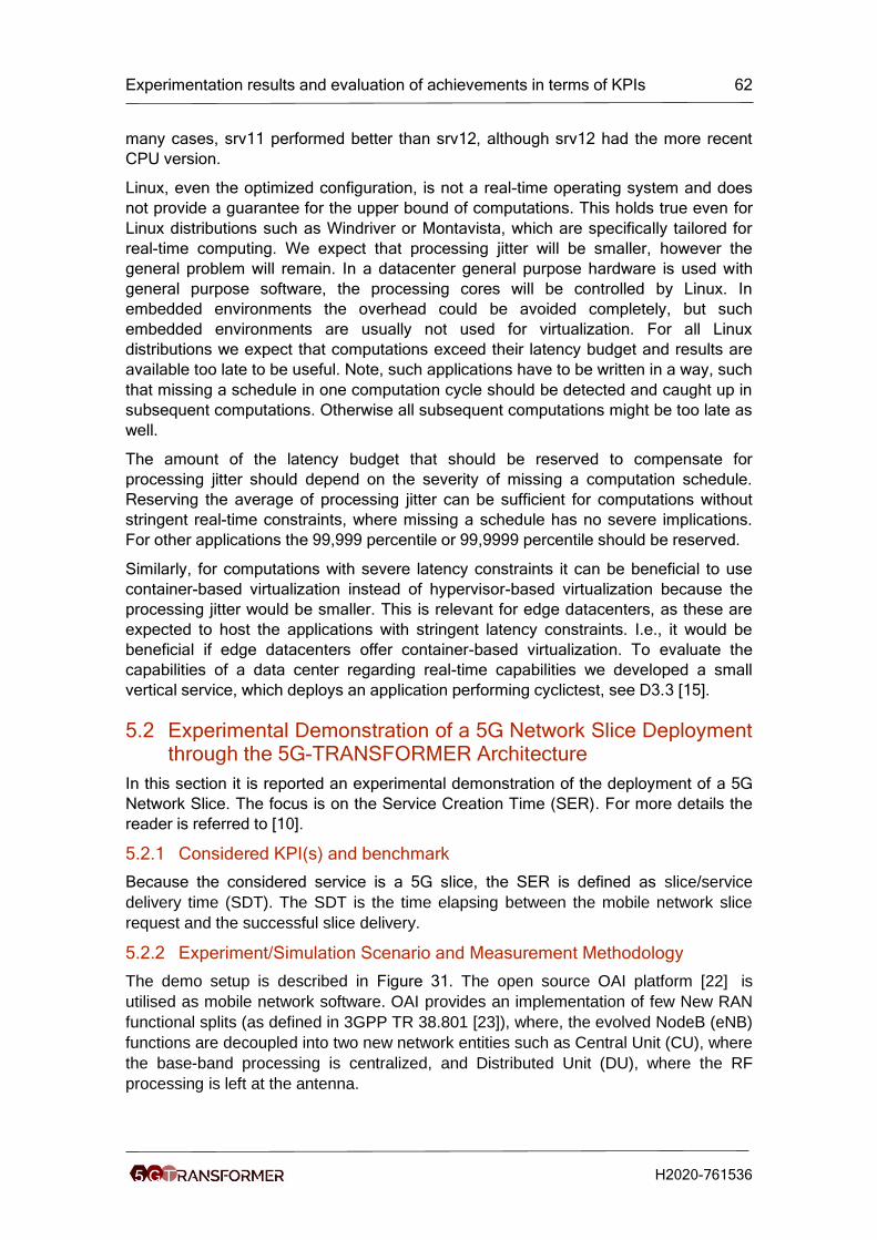
Experimentation results and evaluation of achievements in terms of KPIs 62
H2020-761536
many cases, srv11 performed better than srv12, although srv12 had the more recent
CPU version.
Linux, even the optimized configuration, is not a real-time operating system and does
not provide a guarantee for the upper bound of computations. This holds true even for
Linux distributions such as Windriver or Montavista, which are specifically tailored for
real-time computing. We expect that processing jitter will be smaller, however the
general problem will remain. In a datacenter general purpose hardware is used with
general purpose software, the processing cores will be controlled by Linux. In
embedded environments the overhead could be avoided completely, but such
embedded environments are usually not used for virtualization. For all Linux
distributions we expect that computations exceed their latency budget and results are
available too late to be useful. Note, such applications have to be written in a way, such
that missing a schedule in one computation cycle should be detected and caught up in
subsequent computations. Otherwise all subsequent computations might be too late as
well.
The amount of the latency budget that should be reserved to compensate for
processing jitter should depend on the severity of missing a computation schedule.
Reserving the average of processing jitter can be sufficient for computations without
stringent real-time constraints, where missing a schedule has no severe implications.
For other applications the 99,999 percentile or 99,9999 percentile should be reserved.
Similarly, for computations with severe latency constraints it can be beneficial to use
container-based virtualization instead of hypervisor-based virtualization because the
processing jitter would be smaller. This is relevant for edge datacenters, as these are
expected to host the applications with stringent latency constraints. I.e., it would be
beneficial if edge datacenters offer container-based virtualization. To evaluate the
capabilities of a data center regarding real-time capabilities we developed a small
vertical service, which deploys an application performing cyclictest, see D3.3 [15].
5.2 Experimental Demonstration of a 5G Network Slice Deployment through the 5G-TRANSFORMER Architecture
In this section it is reported an experimental demonstration of the deployment of a 5G
Network Slice. The focus is on the Service Creation Time (SER). For more details the
reader is referred to [10].
5.2.1 Considered KPI(s) and benchmark
Because the considered service is a 5G slice, the SER is defined as slice/service
delivery time (SDT). The SDT is the time elapsing between the mobile network slice
request and the successful slice delivery.
5.2.2 Experiment/Simulation Scenario and Measurement Methodology
The demo setup is described in Figure 31. The open source OAI platform [22] is
utilised as mobile network software. OAI provides an implementation of few New RAN
functional splits (as defined in 3GPP TR 38.801 [23]), where, the evolved NodeB (eNB)
functions are decoupled into two new network entities such as Central Unit (CU), where
the base-band processing is centralized, and Distributed Unit (DU), where the RF
processing is left at the antenna.
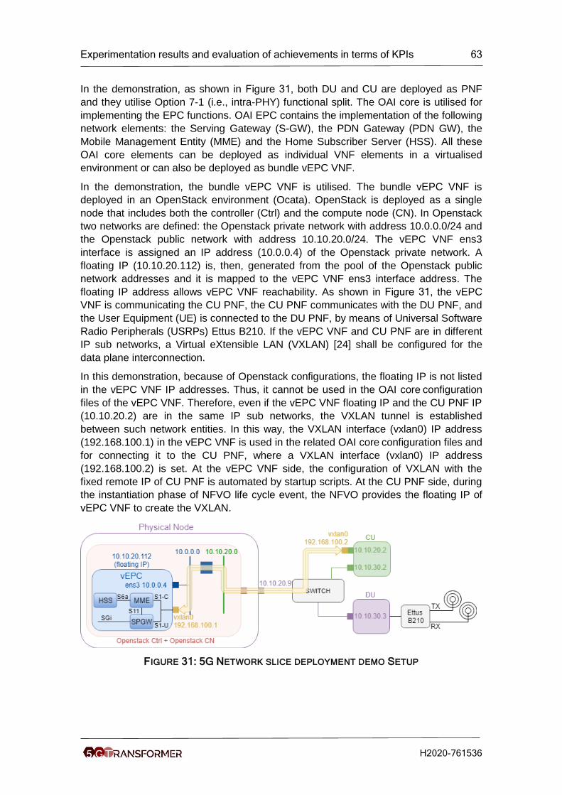
Experimentation results and evaluation of achievements in terms of KPIs 63
H2020-761536
In the demonstration, as shown in Figure 31, both DU and CU are deployed as PNF
and they utilise Option 7-1 (i.e., intra-PHY) functional split. The OAI core is utilised for
implementing the EPC functions. OAI EPC contains the implementation of the following
network elements: the Serving Gateway (S-GW), the PDN Gateway (PDN GW), the
Mobile Management Entity (MME) and the Home Subscriber Server (HSS). All these
OAI core elements can be deployed as individual VNF elements in a virtualised
environment or can also be deployed as bundle vEPC VNF.
In the demonstration, the bundle vEPC VNF is utilised. The bundle vEPC VNF is
deployed in an OpenStack environment (Ocata). OpenStack is deployed as a single
node that includes both the controller (Ctrl) and the compute node (CN). In Openstack
two networks are defined: the Openstack private network with address 10.0.0.0/24 and
the Openstack public network with address 10.10.20.0/24. The vEPC VNF ens3
interface is assigned an IP address (10.0.0.4) of the Openstack private network. A
floating IP (10.10.20.112) is, then, generated from the pool of the Openstack public
network addresses and it is mapped to the vEPC VNF ens3 interface address. The
floating IP address allows vEPC VNF reachability. As shown in Figure 31, the vEPC
VNF is communicating the CU PNF, the CU PNF communicates with the DU PNF, and
the User Equipment (UE) is connected to the DU PNF, by means of Universal Software
Radio Peripherals (USRPs) Ettus B210. If the vEPC VNF and CU PNF are in different
IP sub networks, a Virtual eXtensible LAN (VXLAN) [24] shall be configured for the
data plane interconnection.
In this demonstration, because of Openstack configurations, the floating IP is not listed
in the vEPC VNF IP addresses. Thus, it cannot be used in the OAI core configuration
files of the vEPC VNF. Therefore, even if the vEPC VNF floating IP and the CU PNF IP
(10.10.20.2) are in the same IP sub networks, the VXLAN tunnel is established
between such network entities. In this way, the VXLAN interface (vxlan0) IP address
(192.168.100.1) in the vEPC VNF is used in the related OAI core configuration files and
for connecting it to the CU PNF, where a VXLAN interface (vxlan0) IP address
(192.168.100.2) is set. At the vEPC VNF side, the configuration of VXLAN with the
fixed remote IP of CU PNF is automated by startup scripts. At the CU PNF side, during
the instantiation phase of NFVO life cycle event, the NFVO provides the floating IP of
vEPC VNF to create the VXLAN.
FIGURE 31: 5G NETWORK SLICE DEPLOYMENT DEMO SETUP
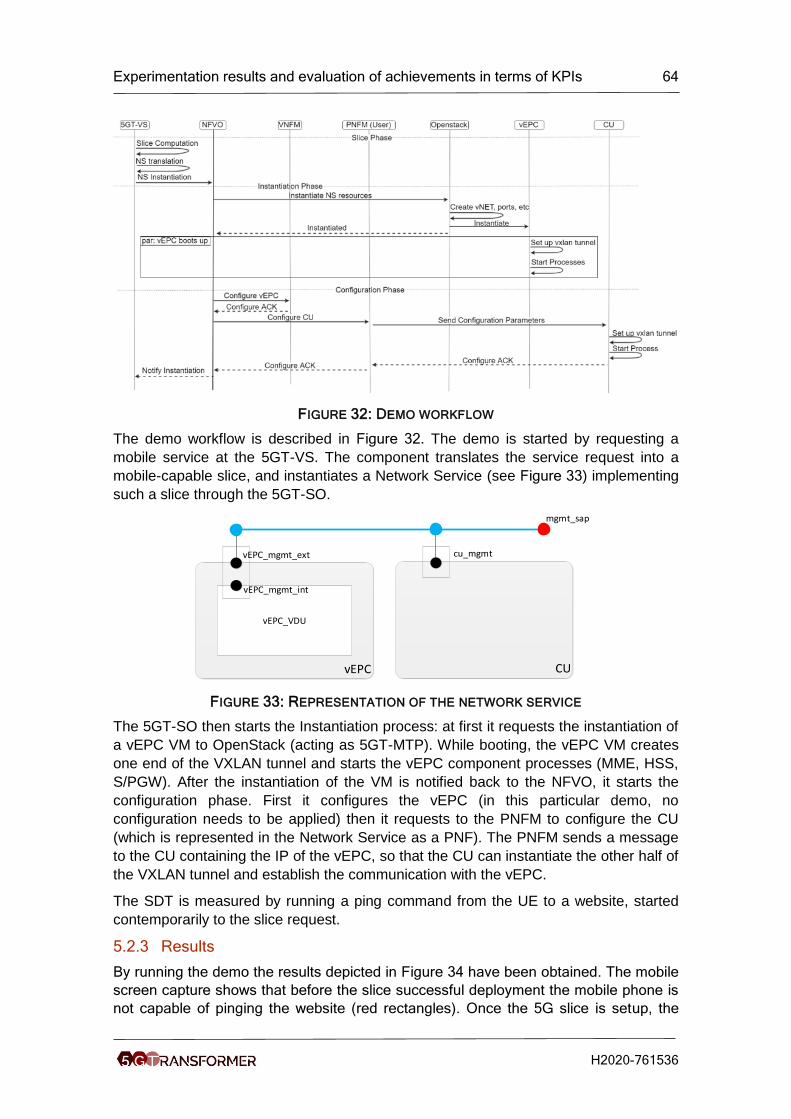
Experimentation results and evaluation of achievements in terms of KPIs 64
H2020-761536
FIGURE 32: DEMO WORKFLOW
The demo workflow is described in Figure 32. The demo is started by requesting a
mobile service at the 5GT-VS. The component translates the service request into a
mobile-capable slice, and instantiates a Network Service (see Figure 33) implementing
such a slice through the 5GT-SO.
CU
cu_mgmt
vEPC
vEPC_VDU
vEPC_mgmt_int
vEPC_mgmt_ext
mgmt_sap
FIGURE 33: REPRESENTATION OF THE NETWORK SERVICE
The 5GT-SO then starts the Instantiation process: at first it requests the instantiation of
a vEPC VM to OpenStack (acting as 5GT-MTP). While booting, the vEPC VM creates
one end of the VXLAN tunnel and starts the vEPC component processes (MME, HSS,
S/PGW). After the instantiation of the VM is notified back to the NFVO, it starts the
configuration phase. First it configures the vEPC (in this particular demo, no
configuration needs to be applied) then it requests to the PNFM to configure the CU
(which is represented in the Network Service as a PNF). The PNFM sends a message
to the CU containing the IP of the vEPC, so that the CU can instantiate the other half of
the VXLAN tunnel and establish the communication with the vEPC.
The SDT is measured by running a ping command from the UE to a website, started
contemporarily to the slice request.
5.2.3 Results
By running the demo the results depicted in Figure 34 have been obtained. The mobile
screen capture shows that before the slice successful deployment the mobile phone is
not capable of pinging the website (red rectangles). Once the 5G slice is setup, the
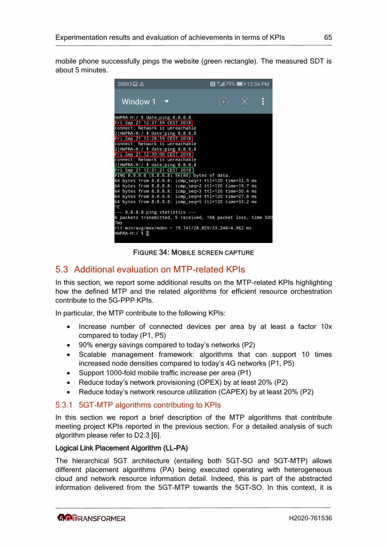
Experimentation results and evaluation of achievements in terms of KPIs 65
H2020-761536
mobile phone successfully pings the website (green rectangle). The measured SDT is
about 5 minutes.
FIGURE 34: MOBILE SCREEN CAPTURE
5.3 Additional evaluation on MTP-related KPIs
In this section, we report some additional results on the MTP-related KPIs highlighting
how the defined MTP and the related algorithms for efficient resource orchestration
contribute to the 5G-PPP KPIs.
In particular, the MTP contribute to the following KPIs:
• Increase number of connected devices per area by at least a factor 10x
compared to today (P1, P5)
• 90% energy savings compared to today’s networks (P2)
• Scalable management framework: algorithms that can support 10 times
increased node densities compared to today’s 4G networks (P1, P5)
• Support 1000-fold mobile traffic increase per area (P1)
• Reduce today’s network provisioning (OPEX) by at least 20% (P2)
• Reduce today’s network resource utilization (CAPEX) by at least 20% (P2)
5.3.1 5GT-MTP algorithms contributing to KPIs
In this section we report a brief description of the MTP algorithms that contribute
meeting project KPIs reported in the previous section. For a detailed analysis of such
algorithm please refer to D2.3 [6].
Logical Link Placement Algorithm (LL-PA)
The hierarchical 5GT architecture (entailing both 5GT-SO and 5GT-MTP) allows
different placement algorithms (PA) being executed operating with heterogeneous
cloud and network resource information detail. Indeed, this is part of the abstracted
information delivered from the 5GT-MTP towards the 5GT-SO. In this context, it is
Experimentation results and evaluation of achievements in terms of KPIs 66
H2020-761536
considered that the 5GT-SO always works with summarized information of the NFVI-
Pop resources (i.e., total available CPU, RAM, Storage) but the WAN infrastructure
enabling the connectivity between remote NFVI-Pop depends on the adopted
abstraction model by the 5GT-MTP.
The goal of the conducted experiments focuses on evaluating the performance (in
terms of served / accepted network service requests) when the 5GT-MTP either
provides abstracted WAN details (i.e., logical links, LLs) to the 5GT-SO or not. In
general, the higher is the amount of accepted network service requests, the better the
algorithm / mechanism performs with respect of the network resource usage. Bearing
this in mind, it is adopted that the network service requests to be accommodate
dynamically arrive / departure to / from the network, respectively. Each request
specifies a VNF Forwarding Group (VNFFG) describing its cloud (i.e., CPU. RAM and
Storage) and network (i.e., bandwidth and maximum end-to-end latency) resource
demands. Accordingly, the objective is that both PAs mechanisms at the 5GT-SO and
5GT-MTP using their corresponding available cloud and network resource information
allows increasing the amount of served (accepted) VNFFG requests via an efficient use
of the network resources. Basically, two main approaches are benchmarked:
i) No Network Information (NNI): in this approach the 5GT-SO’s PA does not
have information related to the LLs from the 5GT-MTP. In other words, the
5GT-SO’s PA only selects the DCs to satisfy the request’s cloud resource
demands. For the inter-DC connectivity, the 5GT-MTP’s PA is the
responsible to compute a feasible path ensuring the bandwidth and latency
requirements.
ii) Abstracted Network Information (ANI): The 5GT-MTP passes the LLs to the
5GT-SO which is stored in the (Abstracted WAN database). This information
allows the 5GT-SO’s PA selecting both the DC and the LLs among those
DCs that satisfy the cloud and network resource demands. If it is not
possible (e.g., current LLs do not allow dealing with the latency
requirement), the 5GT-MTP’s PA is executed (exploiting a more detailed
view of the WAN). Observe that multiple variants for the 5GT-SO’s PA could
be devised and used as discussed in [36][37]
Both NNI and ANI approaches are evaluated over a pool of DCs being interconnected
over a multi-layer WAN network which combines packet and (flexi-grid) optical
switching technologies (see figure below). More details of the considered DC (Nfvi-
Pops) and WAN infrastructure are provided in [37].
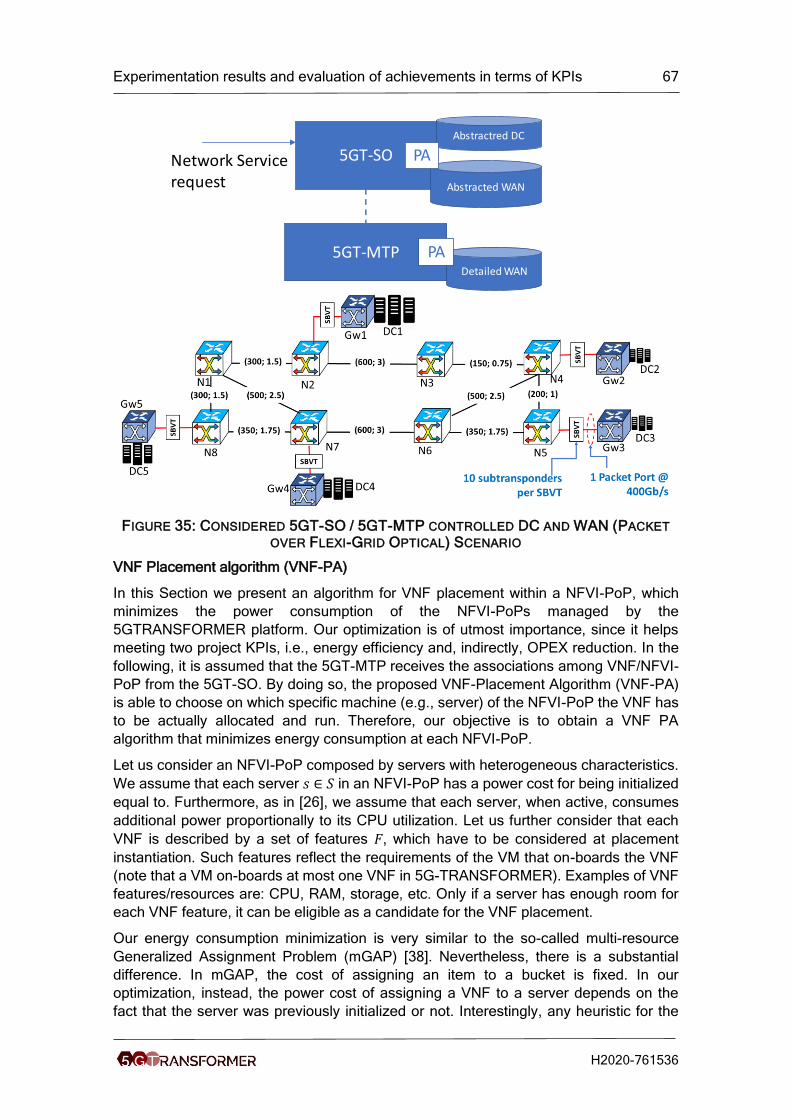
Experimentation results and evaluation of achievements in terms of KPIs 67
H2020-761536
FIGURE 35: CONSIDERED 5GT-SO / 5GT-MTP CONTROLLED DC AND WAN (PACKET
OVER FLEXI-GRID OPTICAL) SCENARIO
VNF Placement algorithm (VNF-PA)
In this Section we present an algorithm for VNF placement within a NFVI-PoP, which
minimizes the power consumption of the NFVI-PoPs managed by the
5GTRANSFORMER platform. Our optimization is of utmost importance, since it helps
meeting two project KPIs, i.e., energy efficiency and, indirectly, OPEX reduction. In the
following, it is assumed that the 5GT-MTP receives the associations among VNF/NFVI-
PoP from the 5GT-SO. By doing so, the proposed VNF-Placement Algorithm (VNF-PA)
is able to choose on which specific machine (e.g., server) of the NFVI-PoP the VNF has
to be actually allocated and run. Therefore, our objective is to obtain a VNF PA
algorithm that minimizes energy consumption at each NFVI-PoP.
Let us consider an NFVI-PoP composed by servers with heterogeneous characteristics.
We assume that each server 𝑠 ∈ 𝑆 in an NFVI-PoP has a power cost for being initialized
equal to. Furthermore, as in [26], we assume that each server, when active, consumes
additional power proportionally to its CPU utilization. Let us further consider that each
VNF is described by a set of features 𝐹, which have to be considered at placement
instantiation. Such features reflect the requirements of the VM that on-boards the VNF
(note that a VM on-boards at most one VNF in 5G-TRANSFORMER). Examples of VNF
features/resources are: CPU, RAM, storage, etc. Only if a server has enough room for
each VNF feature, it can be eligible as a candidate for the VNF placement.
Our energy consumption minimization is very similar to the so-called multi-resource
Generalized Assignment Problem (mGAP) [38]. Nevertheless, there is a substantial
difference. In mGAP, the cost of assigning an item to a bucket is fixed. In our
optimization, instead, the power cost of assigning a VNF to a server depends on the
fact that the server was previously initialized or not. Interestingly, any heuristic for the
5GT-SO
5GT-MTPDetailedWAN
Abstractred DC
Abstracted WAN
PA
PA
Network Servicerequest
Experimentation results and evaluation of achievements in terms of KPIs 68
H2020-761536
mGAP problem that assigns VNFs to servers in a sequential order may also be applied
to our optimization. In our case, when a new VNF placement is performed, it is
sufficient to add the initialization power cost, if needed, to the power cost of assigning
such a VNF to a server.
Therefore, we exploit the state-of-the-art solutions, tailoring them to our specific
problem. As mentioned above, the 5GT-MTP receives from the 5GT-SO the VNF/NFVI-
PoP associations. To exploit off-line heuristics, which perform better than the on-line
ones, we assume that the 5GT-MTP does not executes instantly the decisions of the
5GT-SO. Rather the 5GT-MTP stores them for a time window T. Upon the time window
T expires, the 5GT-MTP places all the VNFs collected and migrates all the VNFs of
non-critical services altogether, with the following algorithm, based on [38]. We assume
that the set of VNFs that needs to be placed/migrated is represented by 𝑉. First, for
each VNF 𝑣 ∈ 𝑉, the set 𝑆𝑣 of servers that can host 𝑣 is obtained. At this stage, if a VNF
𝑣 cannot be placed to any server, the algorithm returns unfeasible solution. Such event
is possible since the SO, when assigning VNFs to NFVI-PoPs, has only aggregate
knowledge on the NFVI-PoP capacity. For this reason, it is possible that no actual
machine can host a VNF that the SO assigned to a specific NFVI-PoP. If instead all
VNFs have at least a server to be assigned to, then the MTP computes VNF
placements. For the 5GT-MTP, a VNF is critical if the energy efficiency difference
between the first and the second best choice for 𝑣 is the largest in 𝑉. Looping over 𝑉,
the 5GT-MTP always assigns the most critical VNF to its best choice up to concluding
VNF placement.
FluidRAN
We propose FluidRAN, a rigorous analytical framework for the optimized configuration
of virtual RAN (vRAN) networks. We model the BS operation as a chain of functions
that successively process the traffic to/from the users. Some of these functions (e.g.,
PDCP in LTE systems) can be implemented in virtual machines (VMs) at radio units
(RUs) or cloud/centralized units (CUs); while others (e.g., turbo(de)coding in LTE
systems) require specific hardware. The function implementation induces a computing
cost that may vary across RUs and CUs, and similarly the selected paths affect the
data transfer expenses. Our framework yields the vRAN configuration (splits and paths)
that minimizes the aggregate operator expenditures.
The features of FluidRAN can be summarized as follows:
• Optimization Framework. FluidRAN introduces an analytical framework for the vRAN design by considering the network and computing resources, and the splits’ requirements. Our solution optimizes the placement of vRAN functions jointly with the data routing; and we leverage the Benders’ decomposition method to enable its derivation for large systems.
• Joint vRAN and MEC Design. FluidRAN analyzes and model the inherent tension among vRAN and MEC. The framework is extended to jointly decide the placement of MEC services and vRAN functions, yielding a configuration that balances performance benefits and associated costs.
Dynamic de/activation of VMs
An algorithm for dynamic de/activation of VMs is under investigation. The flow chart is
shown in Figure 36. As an example, the proposed algorithm exploits monitoring
information to predict the number of active VMs required to serve the expected 5G-
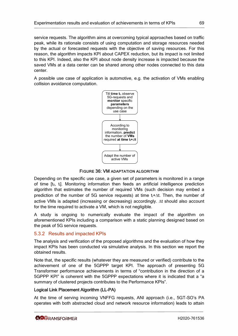
Experimentation results and evaluation of achievements in terms of KPIs 69
H2020-761536
service requests. The algorithm aims at overcoming typical approaches based on traffic
peak, while its rationale consists of using computation and storage resources needed
by the actual or forecasted requests with the objective of saving resources. For this
reason, the algorithm impacts KPI about CAPEX reduction, but its impact is not limited
to this KPI. Indeed, also the KPI about node density increase is impacted because the
saved VMs at a data center can be shared among other nodes connected to this data
center.
A possible use case of application is automotive, e.g. the activation of VMs enabling
collision avoidance computation.
FIGURE 36: VM ADAPTATION ALGORITHM
Depending on the specific use case, a given set of parameters is monitored in a range
of time [t0, ti]. Monitoring information then feeds an artificial intelligence prediction
algorithm that estimates the number of required VMs (such decision may embed a
prediction of the number of 5G service requests) at time ti+t. Then, the number of
active VMs is adapted (increasing or decreasing) accordingly. t should also account
for the time required to activate a VM, which is not negligible.
A study is ongoing to numerically evaluate the impact of the algorithm on
aforementioned KPIs including a comparison with a static planning designed based on
the peak of 5G service requests.
5.3.2 Results and impacted KPIs
The analysis and verification of the proposed algorithms and the evaluation of how they
impact KPIs has been conducted via simulative analysis. In this section we report the
obtained results.
Note that, the specific results (whatever they are measured or verified) contribute to the
achievement of one of the 5GPPP target KPI. The approach of presenting 5G
Transformer performance achievements in terms of “contribution in the direction of a
5GPPP KPI” is coherent with the 5GPPP expectations where it is indicated that a “a
summary of clustered projects contributes to the Performance KPIs”.
Logical Link Placement Algorithm (LL-PA)
At the time of serving incoming VNFFG requests, ANI approach (i.e., 5GT-SO’s PA
operates with both abstracted cloud and network resource information) leads to attain
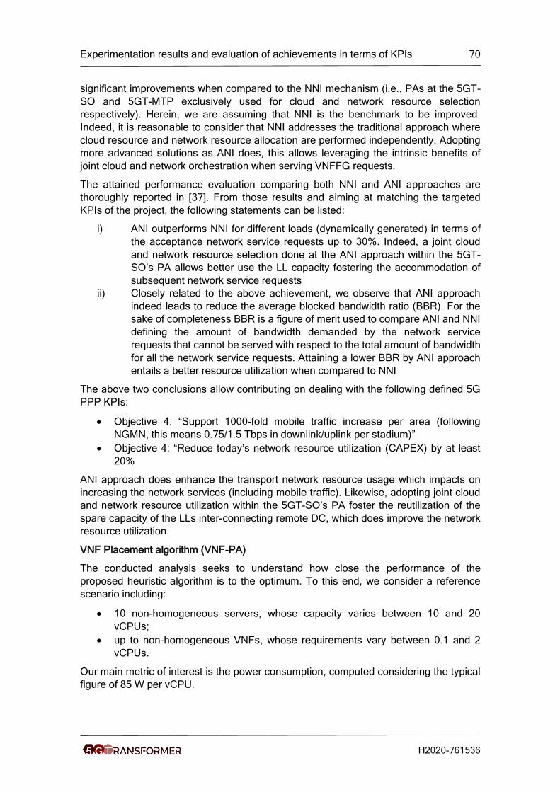
Experimentation results and evaluation of achievements in terms of KPIs 70
H2020-761536
significant improvements when compared to the NNI mechanism (i.e., PAs at the 5GT-
SO and 5GT-MTP exclusively used for cloud and network resource selection
respectively). Herein, we are assuming that NNI is the benchmark to be improved.
Indeed, it is reasonable to consider that NNI addresses the traditional approach where
cloud resource and network resource allocation are performed independently. Adopting
more advanced solutions as ANI does, this allows leveraging the intrinsic benefits of
joint cloud and network orchestration when serving VNFFG requests.
The attained performance evaluation comparing both NNI and ANI approaches are
thoroughly reported in [37]. From those results and aiming at matching the targeted
KPIs of the project, the following statements can be listed:
i) ANI outperforms NNI for different loads (dynamically generated) in terms of
the acceptance network service requests up to 30%. Indeed, a joint cloud
and network resource selection done at the ANI approach within the 5GT-
SO’s PA allows better use the LL capacity fostering the accommodation of
subsequent network service requests
ii) Closely related to the above achievement, we observe that ANI approach
indeed leads to reduce the average blocked bandwidth ratio (BBR). For the
sake of completeness BBR is a figure of merit used to compare ANI and NNI
defining the amount of bandwidth demanded by the network service
requests that cannot be served with respect to the total amount of bandwidth
for all the network service requests. Attaining a lower BBR by ANI approach
entails a better resource utilization when compared to NNI
The above two conclusions allow contributing on dealing with the following defined 5G
PPP KPIs:
• Objective 4: “Support 1000-fold mobile traffic increase per area (following
NGMN, this means 0.75/1.5 Tbps in downlink/uplink per stadium)”
• Objective 4: “Reduce today’s network resource utilization (CAPEX) by at least
20%
ANI approach does enhance the transport network resource usage which impacts on
increasing the network services (including mobile traffic). Likewise, adopting joint cloud
and network resource utilization within the 5GT-SO’s PA foster the reutilization of the
spare capacity of the LLs inter-connecting remote DC, which does improve the network
resource utilization.
VNF Placement algorithm (VNF-PA)
The conducted analysis seeks to understand how close the performance of the
proposed heuristic algorithm is to the optimum. To this end, we consider a reference
scenario including:
• 10 non-homogeneous servers, whose capacity varies between 10 and 20
vCPUs;
• up to non-homogeneous VNFs, whose requirements vary between 0.1 and 2
vCPUs.
Our main metric of interest is the power consumption, computed considering the typical
figure of 85 W per vCPU.
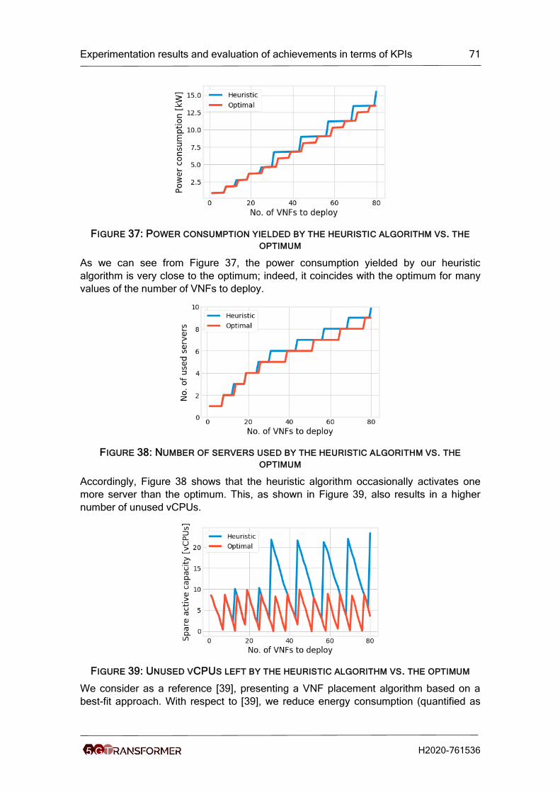
Experimentation results and evaluation of achievements in terms of KPIs 71
H2020-761536
FIGURE 37: POWER CONSUMPTION YIELDED BY THE HEURISTIC ALGORITHM VS. THE
OPTIMUM
As we can see from Figure 37, the power consumption yielded by our heuristic
algorithm is very close to the optimum; indeed, it coincides with the optimum for many
values of the number of VNFs to deploy.
FIGURE 38: NUMBER OF SERVERS USED BY THE HEURISTIC ALGORITHM VS. THE
OPTIMUM
Accordingly, Figure 38 shows that the heuristic algorithm occasionally activates one
more server than the optimum. This, as shown in Figure 39, also results in a higher
number of unused vCPUs.
FIGURE 39: UNUSED VCPUS LEFT BY THE HEURISTIC ALGORITHM VS. THE OPTIMUM
We consider as a reference [39], presenting a VNF placement algorithm based on a
best-fit approach. With respect to [39], we reduce energy consumption (quantified as
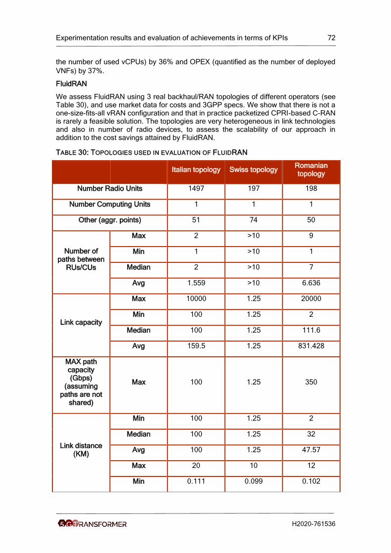
Experimentation results and evaluation of achievements in terms of KPIs 72
H2020-761536
the number of used vCPUs) by 36% and OPEX (quantified as the number of deployed
VNFs) by 37%.
FluidRAN
We assess FluidRAN using 3 real backhaul/RAN topologies of different operators (see Table 30), and use market data for costs and 3GPP specs. We show that there is not a one-size-fits-all vRAN configuration and that in practice packetized CPRI-based C-RAN is rarely a feasible solution. The topologies are very heterogeneous in link technologies and also in number of radio devices, to assess the scalability of our approach in addition to the cost savings attained by FluidRAN.
TABLE 30: TOPOLOGIES USED IN EVALUATION OF FLUIDRAN
Italian topology Swiss topology Romanian topology
Number Radio Units 1497 197 198
Number Computing Units 1 1 1
Other (aggr. points) 51 74 50
Number of paths between
RUs/CUs
Max 2 >10 9
Min 1 >10 1
Median 2 >10 7
Avg 1.559 >10 6.636
Link capacity
Max 10000 1.25 20000
Min 100 1.25 2
Median 100 1.25 111.6
Avg 159.5 1.25 831.428
MAX path capacity (Gbps)
(assuming paths are not
shared)
Max 100 1.25 350
Link distance (KM)
Min 100 1.25 2
Median 100 1.25 32
Avg 100 1.25 47.57
Max 20 10 12
Min 0.111 0.099 0.102
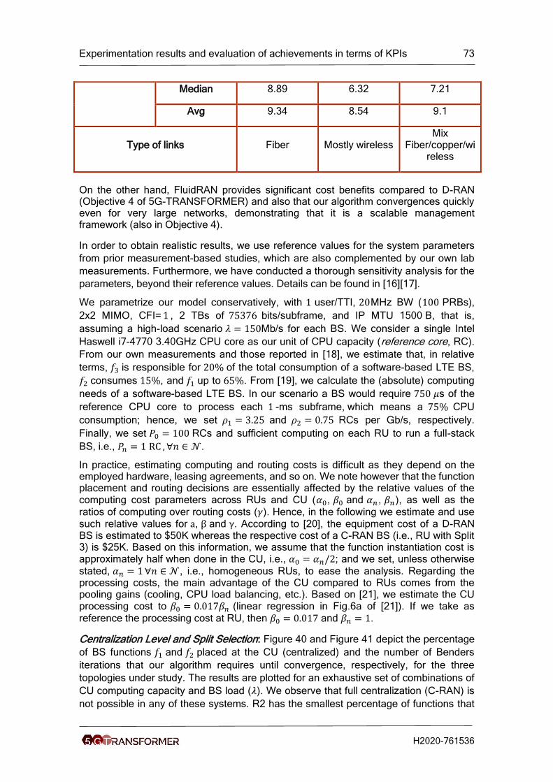
Experimentation results and evaluation of achievements in terms of KPIs 73
H2020-761536
Median 8.89 6.32 7.21
Avg 9.34 8.54 9.1
Type of links Fiber Mostly wireless Mix
Fiber/copper/wireless
On the other hand, FluidRAN provides significant cost benefits compared to D-RAN (Objective 4 of 5G-TRANSFORMER) and also that our algorithm convergences quickly even for very large networks, demonstrating that it is a scalable management framework (also in Objective 4).
In order to obtain realistic results, we use reference values for the system parameters
from prior measurement-based studies, which are also complemented by our own lab
measurements. Furthermore, we have conducted a thorough sensitivity analysis for the
parameters, beyond their reference values. Details can be found in [16][17].
We parametrize our model conservatively, with 1 user/TTI, 20MHz BW (100 PRBs),
2x2 MIMO, CFI=1 , 2 TBs of 75376 bits/subframe, and IP MTU 1500 B, that is,
assuming a high-load scenario 𝜆 = 150Mb/s for each BS. We consider a single Intel
Haswell i7-4770 3.40GHz CPU core as our unit of CPU capacity (reference core, RC).
From our own measurements and those reported in [18], we estimate that, in relative
terms, 𝑓3 is responsible for 20% of the total consumption of a software-based LTE BS,
𝑓2 consumes 15%, and 𝑓1 up to 65%. From [19], we calculate the (absolute) computing
needs of a software-based LTE BS. In our scenario a BS would require 750 𝜇s of the
reference CPU core to process each 1 -ms subframe, which means a 75% CPU
consumption; hence, we set 𝜌1 = 3.25 and 𝜌2 = 0.75 RCs per Gb/s, respectively.
Finally, we set 𝑃0 = 100 RCs and sufficient computing on each RU to run a full-stack
BS, i.e., 𝑃𝑛 = 1 RC , ∀𝑛 ∈ 𝒩.
In practice, estimating computing and routing costs is difficult as they depend on the employed hardware, leasing agreements, and so on. We note however that the function placement and routing decisions are essentially affected by the relative values of the computing cost parameters across RUs and CU (𝛼0, 𝛽0 and 𝛼𝑛, 𝛽𝑛), as well as the
ratios of computing over routing costs (𝛾). Hence, in the following we estimate and use such relative values for a, β and γ. According to [20], the equipment cost of a D-RAN BS is estimated to $50K whereas the respective cost of a C-RAN BS (i.e., RU with Split 3) is $25K. Based on this information, we assume that the function instantiation cost is approximately half when done in the CU, i.e., 𝛼0 = 𝛼𝑛/2; and we set, unless otherwise
stated, 𝛼𝑛 = 1 ∀𝑛 ∈ 𝒩, i.e., homogeneous RUs, to ease the analysis. Regarding the processing costs, the main advantage of the CU compared to RUs comes from the pooling gains (cooling, CPU load balancing, etc.). Based on [21], we estimate the CU processing cost to 𝛽0 = 0.017𝛽𝑛 (linear regression in Fig.6a of [21]). If we take as
reference the processing cost at RU, then 𝛽0 = 0.017 and 𝛽𝑛 = 1.
Centralization Level and Split Selection: Figure 40 and Figure 41 depict the percentage
of BS functions 𝑓1 and 𝑓2 placed at the CU (centralized) and the number of Benders
iterations that our algorithm requires until convergence, respectively, for the three
topologies under study. The results are plotted for an exhaustive set of combinations of
CU computing capacity and BS load (𝜆). We observe that full centralization (C-RAN) is
not possible in any of these systems. R2 has the smallest percentage of functions that
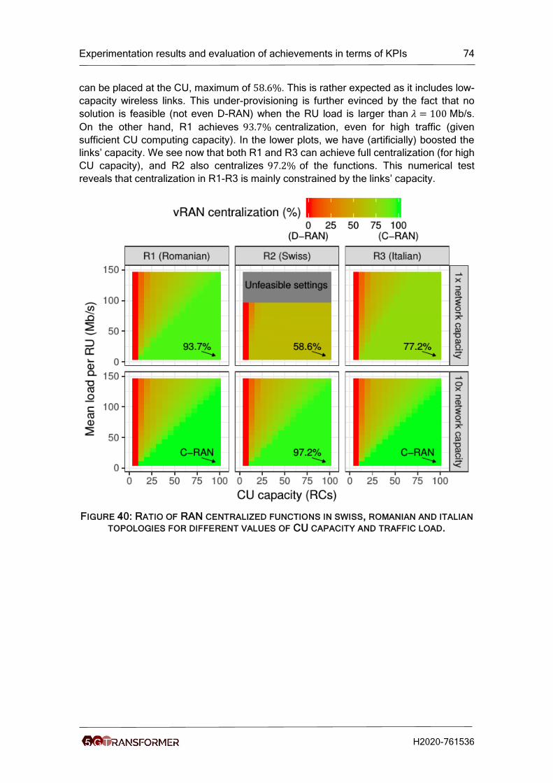
Experimentation results and evaluation of achievements in terms of KPIs 74
H2020-761536
can be placed at the CU, maximum of 58.6%. This is rather expected as it includes low-
capacity wireless links. This under-provisioning is further evinced by the fact that no
solution is feasible (not even D-RAN) when the RU load is larger than 𝜆 = 100 Mb/s.
On the other hand, R1 achieves 93.7% centralization, even for high traffic (given
sufficient CU computing capacity). In the lower plots, we have (artificially) boosted the
links’ capacity. We see now that both R1 and R3 can achieve full centralization (for high
CU capacity), and R2 also centralizes 97.2% of the functions. This numerical test
reveals that centralization in R1-R3 is mainly constrained by the links’ capacity.
FIGURE 40: RATIO OF RAN CENTRALIZED FUNCTIONS IN SWISS, ROMANIAN AND ITALIAN
TOPOLOGIES FOR DIFFERENT VALUES OF CU CAPACITY AND TRAFFIC LOAD.
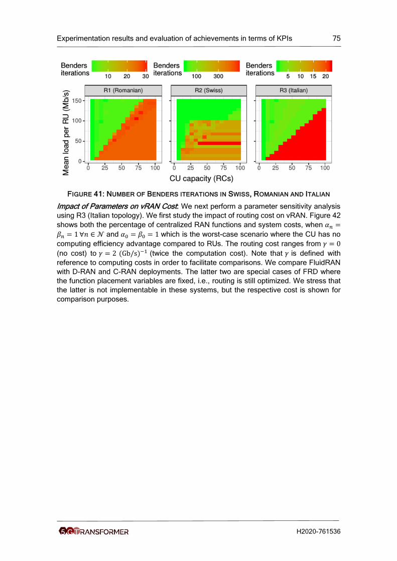
Experimentation results and evaluation of achievements in terms of KPIs 75
H2020-761536
FIGURE 41: NUMBER OF BENDERS ITERATIONS IN SWISS, ROMANIAN AND ITALIAN
Impact of Parameters on vRAN Cost: We next perform a parameter sensitivity analysis
using R3 (Italian topology). We first study the impact of routing cost on vRAN. Figure 42
shows both the percentage of centralized RAN functions and system costs, when 𝛼𝑛 =
𝛽𝑛 = 1 ∀𝑛 ∈ 𝒩 and 𝛼0 = 𝛽0 = 1 which is the worst-case scenario where the CU has no
computing efficiency advantage compared to RUs. The routing cost ranges from 𝛾 = 0
(no cost) to 𝛾 = 2 (Gb/s)−1 (twice the computation cost). Note that 𝛾 is defined with
reference to computing costs in order to facilitate comparisons. We compare FluidRAN
with D-RAN and C-RAN deployments. The latter two are special cases of FRD where
the function placement variables are fixed, i.e., routing is still optimized. We stress that
the latter is not implementable in these systems, but the respective cost is shown for
comparison purposes.
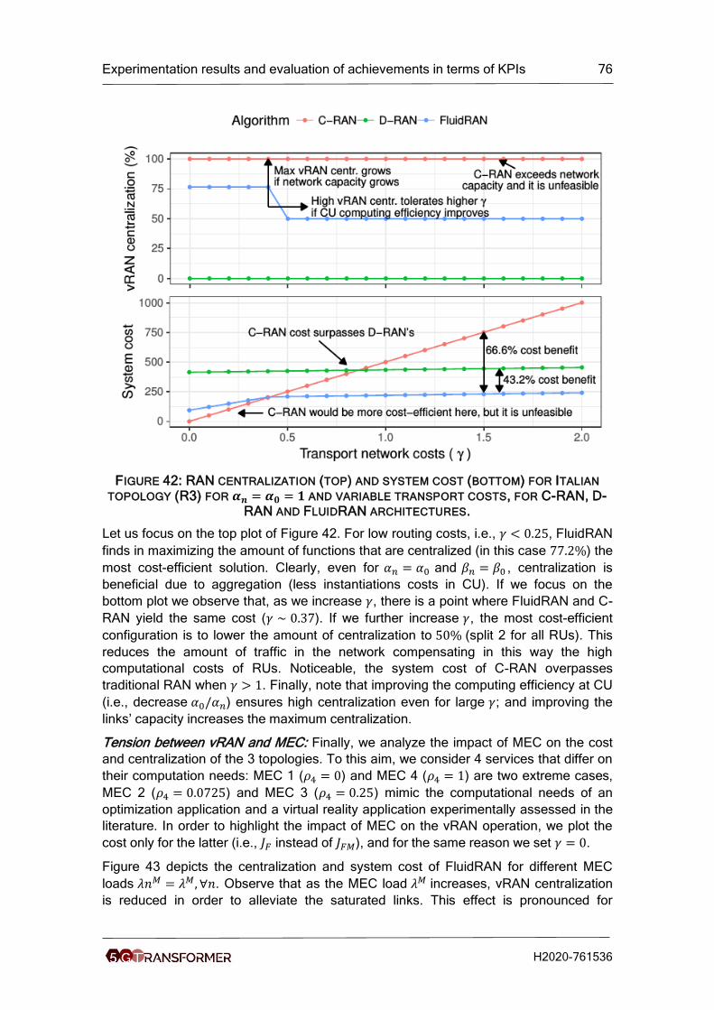
Experimentation results and evaluation of achievements in terms of KPIs 76
H2020-761536
FIGURE 42: RAN CENTRALIZATION (TOP) AND SYSTEM COST (BOTTOM) FOR ITALIAN
TOPOLOGY (R3) FOR 𝜶𝒏 = 𝜶𝟎 = 𝟏 AND VARIABLE TRANSPORT COSTS, FOR C-RAN, D-RAN AND FLUIDRAN ARCHITECTURES.
Let us focus on the top plot of Figure 42. For low routing costs, i.e., 𝛾 < 0.25, FluidRAN
finds in maximizing the amount of functions that are centralized (in this case 77.2%) the
most cost-efficient solution. Clearly, even for 𝛼𝑛 = 𝛼0 and 𝛽𝑛 = 𝛽0 , centralization is
beneficial due to aggregation (less instantiations costs in CU). If we focus on the
bottom plot we observe that, as we increase 𝛾, there is a point where FluidRAN and C-
RAN yield the same cost (𝛾 ∼ 0.37). If we further increase 𝛾, the most cost-efficient
configuration is to lower the amount of centralization to 50% (split 2 for all RUs). This
reduces the amount of traffic in the network compensating in this way the high
computational costs of RUs. Noticeable, the system cost of C-RAN overpasses
traditional RAN when 𝛾 > 1. Finally, note that improving the computing efficiency at CU
(i.e., decrease 𝛼0/𝛼𝑛) ensures high centralization even for large 𝛾; and improving the
links’ capacity increases the maximum centralization.
Tension between vRAN and MEC: Finally, we analyze the impact of MEC on the cost
and centralization of the 3 topologies. To this aim, we consider 4 services that differ on
their computation needs: MEC 1 (𝜌4 = 0) and MEC 4 (𝜌4 = 1) are two extreme cases,
MEC 2 (𝜌4 = 0.0725) and MEC 3 (𝜌4 = 0.25) mimic the computational needs of an
optimization application and a virtual reality application experimentally assessed in the
literature. In order to highlight the impact of MEC on the vRAN operation, we plot the
cost only for the latter (i.e., 𝐽𝐹 instead of 𝐽𝐹𝑀), and for the same reason we set 𝛾 = 0.
Figure 43 depicts the centralization and system cost of FluidRAN for different MEC
loads 𝜆𝑛𝑀 = 𝜆𝑀, ∀𝑛. Observe that as the MEC load 𝜆𝑀 increases, vRAN centralization
is reduced in order to alleviate the saturated links. This effect is pronounced for
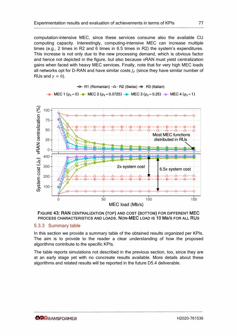
Experimentation results and evaluation of achievements in terms of KPIs 77
H2020-761536
computation-intensive MEC, since these services consume also the available CU
computing capacity. Interestingly, computing-intensive MEC can increase multiple
times (e.g., 2 times in R2 and 6 times in 6.5 times in R2) the system’s expenditures.
This increase is not only due to the new processing demand, which is obvious factor
and hence not depicted in the figure, but also because vRAN must yield centralization
gains when faced with heavy MEC services. Finally, note that for very high MEC loads
all networks opt for D-RAN and have similar costs 𝐽𝐹 (since they have similar number of
RUs and 𝛾 = 0).
FIGURE 43: RAN CENTRALIZATION (TOP) AND COST (BOTTOM) FOR DIFFERENT MEC
PROCESS CHARACTERISTICS AND LOADS. NON-MEC LOAD IS 10 MB/S FOR ALL RUS
5.3.3 Summary table
In this section we provide a summary table of the obtained results organized per KPIs.
The aim is to provide to the reader a clear understanding of how the proposed
algorithms contribute to the specific KPIs.
The table reports simulations not described in the previous section, too, since they are
at an early stage yet with no concreate results available. More details about these
algorithms and related results will be reported in the future D5.4 deliverable.
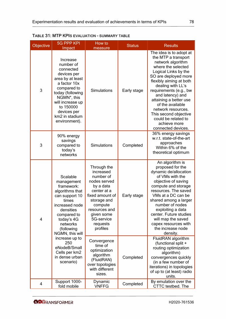
Experimentation results and evaluation of achievements in terms of KPIs 78
H2020-761536
TABLE 31: MTP KPIS EVALUATION – SUMMARY TABLE
Objective 5G PPP KPI
Impact How to
measure Status Results
3
Increase number of connected devices per
area by at least a factor 10x compared to
today (following NGMN*, this
will increase up to 150000
devices per km2 in stadium environment).
Simulations Early stage
The idea is to adopt at the MTP a transport network algorithm where the selected Logical Links by the
SO are deployed more flexibly aiming at both
dealing with LL’s requirements (e.g., bw
and latency) and attaining a better use
of the available network resources.
This second objective could be related to
achieve more connected devices.
3
90% energy savings
compared to today’s
networks
Simulations Completed
36% energy savings w.r.t. state-of-the-art
approaches Within 6% of the
theoretical optimum
4
Scalable management framework:
algorithms that can support 10
times increased node
densities compared to today’s 4G networks (following
NGMN, this will increase up to
250 eNodeB/Small Cells per km2 in dense urban
scenario)
Through the increased number of
nodes served by a data
center at a fixed amount of
storage and compute
resources and given some 5G-service requests profiles
Early stage
An algorithm is proposed for the
dynamic de/allocation of VMs with the
objective of saving compute and storage resources. The saved VMs at a DC can be
shared among a larger number of nodes exploiting a data
center. Future studies will map the saved
capex resources with the increase node
density.
Convergence time of
optimization algorithm
(FluidRAN) over topologies
with different sizes.
Completed
FluidRAN algorithm (functional split +
routing optimization algorithm)
convergences quickly (in a few number of
iterations) in topologies of up to (at least) radio
units.
4 Support 1000-
fold mobile Dynamic VNFFG
Completed By emulation over the
CTTC testbed. The

Experimentation results and evaluation of achievements in terms of KPIs 79
H2020-761536
traffic increase per area (following
NGMN, this means 0.75/1.5
Tbps in downlink/uplink
per stadium)
requests are generated and
need to be accommodated over a myriad of NFVI-PoPs
(DCs) interconnected
by a packet-optical WAN
infrastructure. The
comparison is made between ANI and NNI approaches
with respect to the acceptance
ratio
joint selection of cloud and network resources
at the 5GT-SO’s PA allows increasing up to 30% the acceptance ratio when compared to the performance
done by NNI Such an improvement on the
acceptance ratio leads to increase the
transport capacity within the WAN, and thus supporting the
increase of any carried traffic (e.g., mobile)
4
Reduce today’s network
provisioning (OPEX) by at
least 20%
Simulations, considering the
number of active virtual
machines
Completed
37% savings w.r.t. state-of-the-art
approaches (*)
Within 7% of the
theoretical optimum
4
Reduce today’s network resource utilization
(CAPEX) by at least 20%
Dynamic VNFFG
requests are generated and
need to be accommodated over a myriad of NFVI-PoPs
(DCs) interconnected
by a packet-optical WAN
infrastructure. The
comparison is made between ANI and NNI approaches with to the BBR metric
Completed
By emulation over the CTTC testbed.
Adopting a joint cloud and network resource computation as in ANI
does improve up to 33% of the BBR. In
other words, enhances the network resource utilization with respect
to the NNI
CAPEX and OPEX
(aggregated) savings over a
purely distributed RAN (no functional
splits) and a
FluidRAN algorithm achieves up to 43.2%
cost improvement over standard distributed
RAN. C-RAN (which is an unfeasible
configuration due to transport constraints) has cost savings only
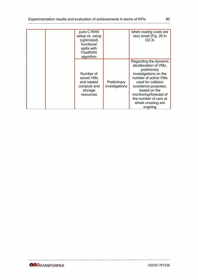
Experimentation results and evaluation of achievements in terms of KPIs 80
H2020-761536
pure C-RAN setup vs. using
(optimized) functional splits with FluidRAN algorithm
when routing costs are very small (Fig. 26 in
D2.3)
Number of saved VMs and related
compute and storage
resources
Preliminary investigations
Regarding the dynamic de/allocation of VMs,
preliminary investigations on the
number of active VMs used for collision
avoidance purposes, based on the
monitoring/forecast of the number of cars at
street crossing are ongoing
Experimentation results and evaluation of achievements in terms of KPIs 81
H2020-761536
6 Summary In this deliverable, we have presented, in Section 2, both the 5G-PPP performance
KPIs and 5G-TRANSFORMER KPIs, as well as the mapping among them. In Section
3, we have described the PoCs of the use cases, namely: the Automotive,
Entertainment, E-Health, E-Industry, and MNO/MVNO use cases. Most of these use
cases have been demonstrated at EuCNC 2019 (June 2019). The experiments,
methodologies, measurements and results are highlighted in Section 4. For each use
case, KPIs have been seelcted among the the 5G-TRANSFORMER KPIs. These KPIs
are benchmarked and the evaluated through experiments. The results of these KPI
evaluations are explained and analysed. These evaluations have shown the beneifts of
the 5G-TRANSFORMER system for orchestration and automation of service
deployments. In Section 5, we have provided additional KPI evaluation for real-time
computation in virtualized environments, the demonstration of network slice
deployments through the 5G-TRANSFORMER architecture, as well as the contribution
of work package 2 algorithms in the obtained KPIs.
In summary, this deliverable evaluates most of the 5G-TRANSFORMER framework
features done so far.
This deliverable validates the following achievements :
• Design and implementation of the 5GT-VS, as well as its integration on sites
including 5TONIC.
• Design and implementation of the 5GT-SO, as well as its integration on 5TONIC
site.
• IIntegration of the 5GT-VS and 5GT-SO.
• Algorithms for arbitration of services, resource shortage, service decomposition,
translation between VSBs and NSTs, and NSTs with NSDs.
• Algorithms for VNF placement, service scaling, and service composition for the
5GT-SO.
• Design and implementation of the 5GT-MTP with plugins for VIMs (Openstack,
Kubernetes, and Xen), WIMs (SDN controllers), radio, and MEC.
• Algorithms for VNF placement by the 5GT-MTP.
Integration of the 5GT-SO and 5GT-MTP and the different plugins of the 5GT-MTP is
ongoing in the selected sites. In addition to these activities, we will perform service
federation and autoscaling of network services. The corresponding validation and
evaluation activities will be reported in the next deliverable D5.4.
Experimentation results and evaluation of achievements in terms of KPIs 82
H2020-761536
7 References [1] 5G-TRANSFORMER, “D5.2, Integration and proofs of concept plan,” November
2018.
[2] 5G-TRANSFORMER, “D1.1, Report on vertical requirements and use cases,”
November 2017.
[3] 5G-PPP, “Contractual Arrangement Setting up a Public Private Partnership in the
Area of Advanced 5G Network Infrastructure for te Future Internet between the
European Union and the 5G Infrastructure Association,” December 2013, available
at https://5g-ppp.eu/contract/
[4] 5G-PPP, “Use cases and performance evaluation modelling,” version 1.0, April
2016, available at https://5g-ppp.eu/white-papers/
[5] P. Iovanna, F. Cavaliere, F. Testa, S. Stracca, G. Bottari, F. Ponzini, A. Bianchi,
and R. Sabella, “Future Proof Optical Network Infrastructure for 5G Transport,”
IEEE/OSA Journal of Optical Commununications and Networking, vol. 8, no. 12,
pp. B80-B92, 2016.
[6] 5G-TRANSFORMER, “D2.3, Final design and implementation report on the MTP,”
May 2019.
[7] Tomasz Szot et al, “Comparative analysis of positioning accuracy of Samsung
Galaxy smartphones in stationary measurements,” vol. 14, no. 4, 2019.
[8] T. Szigeti, “QoS Requirements of Video > Quality of Service Design Overview,”
17 December 2004,
http://www.ciscopress.com/articles/article.asp?p=357102&seqNum=2
[9] Huawei, “Whitepaper on the VR-Oriented Bearer Network Requirement,” 2016.
[10] M Capitani, F Giannone, S Fichera, A Sgambelluri, K Kondepu, E Kraja, B Martini,
G Landi, L Valcarenghi, “Experimental Demonstration of a 5G Network Slice
Deployment Through the 5G-Transformer Architecture”, in 2018 European
Conference on Optical Communication (ECOC), Rome, Italy, September 23-27.
[11] Configuring and tuning HP ProLiant Servers for low-latency applications, available
at
https://h50146.www5.hpe.com/products/software/oe/linux/mainstream/support/whit
epaper/pdfs/c01804533-2014-nov.pdf
[12] Intel BIOS Implementation Test Suite (BITS), https://biosbits.org/
[13] The kernel’s command-line parameters,
https://www.kernel.org/doc/html/v4.14/admin-guide/kernel-parameters.html
[14] cyclictest - High resolution test program,
http://manpages.ubuntu.com/manpages/cosmic/man8/cyclictest.8.html
[15] 5G-TRANSFORMER, “D3.3, Final design and implementation report on the
Vertical Slicer (report)”, Mai 2019.
[16] A. Garcia-Saavedra, X. Costa-Perez, D. J. Leith, G. Iosifidis, "FluidRAN: Optimized
vRAN/MEC Orchestration", In IEEE Conference on Computer Communications
(INFOCOM), Honolulu, HI, USA, April 16-19, 2018.
Experimentation results and evaluation of achievements in terms of KPIs 83
H2020-761536
[17] A. Garcia-Saavedra, G. Iosifidis, X. Costa-Perez, D. J. Leith, "Joint Optimization of
Edge Computing Architectures and Radio Access Networks", In IEEE Journal on
Selected Areas in Communications, vol. 36, no.11, pp 2433-2443, 2018.
[18] C. Y. Yeoh, M. H. Mokhtar, A. A. A. Rahman, A. K. Samingan, “Performance study
of LTE experimental testbed using OpenAirInterface,” in Proceeding of the 18th
IEEE International Conference on Advanced Communications Technology
(ICACT), Phoenix Park, PyeongChang, Korea, pp. 617–622, January 31-Febrary 3,
2016.
[19] N. Nikaein, “Processing Radio Access Network Functions in the Cloud: Critical
Issues and Modeling”, Proceedings of the 6th ACM International Workshop on
Mobile Cloud Computing and Services (MCS), Paris, France, September 11, 2015.
[20] V. Suryaprakash, P. Rost, G. P. Fettweis, “Are Heterogeneous Cloud-Based Radio
Access Networks Cost Effective?”, in IEEE Journal on Selected Areas in
Communications (JSAC), vol. 33, no. 10, pp. 2239-2251, 2015.
[21] P. Rost, S. Talarico, M. C. Valenti, “The Complexity-Rate Tradeoff of Centralized
Radio Access Networks”, IEEE Transaction on Wireless Communications, vo. 14,
no. 11, pp. 6164-6176, 2015.
[22] http://www.openairinterface.org
[23] 3GPP TR 38.801, “Study on new radio access technology: Radio access
architecture and interfaces”, Tech. Rep., V14.0.0, 03 2017, release 14.
[24] M. Mahalingam et al., "Virtual extensible local area network (VXLAN): A framework
for overlaying virtualized layer 2 networks over layer 3 networks", IETF, RFC 7348,
August, 2014.
[25] C. Pham, N. H. Tran, S. Ren, W. Saad and C. S. Hong, “Traffic-aware and Energy-
efficient vNF Placement for Service Chaining: Joint Sampling and Matching
Approach,” IEEE Transactions on Services Computing, 2017.
[26] A. Beloglazov, and B. Rajkumar. "Optimal online deterministic algorithms and
adaptive heuristics for energy and performance efficient dynamic consolidation of
virtual machines in cloud data centers," in Journal of Concurrency and
Computation: Practice and Experience, vo. 24, no. 13, pp. 1397-1420, 2012.
[27] B. Gavish, H. Pirkul, "Algorithms for the Multi-Resource Generalized Assignment
Problem," Management Science, Vol. 37, No. 6, pp. 695-713, 1991.
[28] IEEE Standards Association, “ Standard for Information Technology -
Telecommunications and Information Exchange between Systems - Local and
Metropolitan Area Networks - Specific Requirements Part 11 - Amendment 6:
Wireless Access in Vehicular Environment,” 2010.
[29] IEEE Standards Association, “Standard for Information Technology -
Telecommunications and Information Exchange between Systems - Local and
Metropolitan Area Networks - Specific Requirements - Part 11: Wireless LAN
Medium Access Control (MAC) and Physical Layer (PHY) Specifications,” 2012.
[30] ETSI EN 302 663, "Intelligent Transport Systems (ITS); Access layer specification
for Intelligent Transport Systems operating in the 5 GHz frequency band," Final
Draft, V1.2.1, May 2013.
Experimentation results and evaluation of achievements in terms of KPIs 84
H2020-761536
[31] ETSI EN 302 637-2, “Intelligent Transport Systems (ITS); Vehicular
Communications; Basic Set of Applications; Part 2: Specification of Cooperative
Awareness Basic Service,” Final Draft, V1.3.2, November 2014.
[32] Z. Xu, X. Li, X. Zhao, M. H. Zang, and Z. Wang, “Dsrc versus 4g-lte for connected
vehicle applications: A study on field experiments of vehicular communication
performance,” Journal of Advanced Transportation, vo. 435, 2017.
[33] Z. H. Mir and F. Filali, “Lte and ieee 802.11p for vehicular networking: a
performance evaluation,” EURASIP Journal on Wireless Communications and
Networking, vo. 2014, no. 1, pp. 89, May 2014.
[34] http://simulte.com/add_veins.html
[35] M. Behrisch, L. Bieker, J. Erdmann, and D. Krajzewicz, “Sumo–simulation of urban
mobility: an overview,” Procedings of the 3rd International Conference on
Advances in System Simulation (SIMUL 2011), Barcelona, Spain, 2011.
[36] 5G-TRANSFORMER, "D4.3, Final design and implementation report on service
orchestration, federation and monitoring platform", May 2019.
[37] S. Fichera et al., "Latency-aware resource orchestration in SDN-based packet over
optical flexi-grid transport networks," in IEEE/OSA Journal of Optical
Communications and Networking, vol. 11, no. 4, pp. B83-B96, April 2019.
[38] B. Gavish and H. Pirkul, "Algorithms for the multi-resource generalized assignment
problem," Journal of Management science, vo. 37, no. 6, pp. 695-713, 1991.
[39] C. Pham, N. H. Tran, S. Ren, W. Saad and C. S. Hong, "Traffic-aware and Energy-
efficient vNF Placement for Service Chaining: Joint Sampling and Matching
Approach," in IEEE Transactions on Services Computing, 2017.
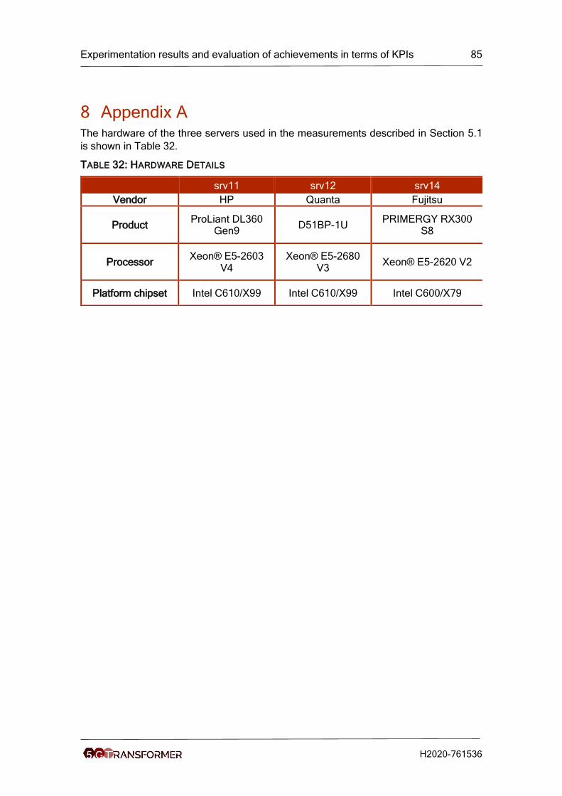
Experimentation results and evaluation of achievements in terms of KPIs 85
H2020-761536
8 Appendix A The hardware of the three servers used in the measurements described in Section 5.1
is shown in Table 32.
TABLE 32: HARDWARE DETAILS
srv11 srv12 srv14
Vendor HP Quanta Fujitsu
Product ProLiant DL360
Gen9 D51BP-1U
PRIMERGY RX300 S8
Processor Xeon® E5-2603
V4 Xeon® E5-2680
V3 Xeon® E5-2620 V2
Platform chipset Intel C610/X99 Intel C610/X99 Intel C600/X79