D4h-Final report on WP4 - emotion-research.netemotion-research.net/projects/humaine/deliverables/D4h-Final report... · D4h 2 IST FP6 Contract no. 507422 IST project contract no

D4h: Final report on WP4

Workpackage 4 Deliverable

Date: 30th January 2008

D4h

IST FP6 Contract no. 507422 2

IST project contract no. 507422

Project title HUMAINE Human-Machine Interaction Network on Emotions

Contractual date of delivery January 30, 2008

Actual date of delivery February 14, 2008

Deliverable number D4h

Deliverable title Final report on WP4

Type Report

Number of pages 48

WP contributing to thedeliverable

WP 4

Task leader ICCS-NTUA

Author(s) S. Abrilian, V. Aharonson, N. Amir, E. Andre, S. Asteriadis, A. Batliner, G. Caridakis, A. Cerekovic, R.Cowie, L. Devillers, D. Grandjean, F. Hoenig, S. Ioannou,K. Karpouzis, L. Kessous, J. Kim, S. Kollias, L. Lamel, M.Mancini, JC. Martin, E. McMahon, I. Pandžić, C. Pelachaud, A. Raouzaiou, B. Schuller, L. Vidrascu, T. Vogt, G. Zorić

EC Project Officer Philippe Gelin

Address of lead author: Stefanos Kollias

Computer Science Department School of Electrical and Computer Engineering National Technical University of Athens Zografou 15780, Athens, Greece

D4h


Table of Contents

1 THE PLACE OF THIS REPORT WITHIN HUMAINE AND THE WP4 EXEMPLAR ................................................................................................................. 5

2 BRIEF OVERVIEW OF WORKPACKAGE 4 AND ITS EXEMPLAR ................... 7

2.1 Introduction .................................................................................................................. 7

2.2 Sub-group 1: Speech analysis and recognition .......................................................... 7

2.3 Sub-group 2: Visual analysis and recognition ........................................................... 8

2.4 Sub-group 3: Analysis and recognition of physiological features ............................ 9

2.5 Sub-group 4: Multimodal recognition ........................................................................ 9

3 ADVANCING THE STATE OF THE ART ........................................................... 11

3.1 The CEICES initiative – results and findings .......................................................... 11 3.1.1 Trying different feature sets and classification approaches ................................. 11 3.1.2 The impact of erroneous F0 extraction [2] ........................................................... 12 3.1.3 Laryngealizations (voice quality) and emotion [4] .............................................. 12 3.1.4 The impact of feature type and functionals on classification performance [9] .... 12 3.1.5 Emotion recognition with reverberated and noisy speech [8] .............................. 13

3.2 Real-time/detailed facial feature extraction ............................................................. 13 3.2.1 Multi-cue facial feature extraction ....................................................................... 13 3.2.2 Real time feature extraction – estimation of head pose and eye gaze .................. 16

3.3 Dynamic recognition of naturalistic affective states ............................................... 19 3.3.1 Classification ........................................................................................................ 20 3.3.2 Results and comparison ........................................................................................ 22

3.4 Multimodal adaptation and retraining .................................................................... 27 3.4.1 An adaptive neural network architecture ............................................................. 28 3.4.2 Detecting the need for adaptation ......................................................................... 30 3.4.3 Experiments .......................................................................................................... 31

3.5 Biosignals as a Baseline Channel .............................................................................. 33 3.5.1 Relation, dependencies and correlation of bio signals with other modalities ...... 34 3.5.2 Augsburg Biosignal Toolbox (AuBT) .................................................................. 35

D4h


4 LINKS TO OTHER WORK PACKAGES ............................................................ 36

4.1 Annotation of large databases – expressivity features ............................................ 36 4.1.1 Calculation of gesture expressivity features ......................................................... 38

4.2 Synthesis of expressive gestures ................................................................................ 39 4.2.1 Implementation ..................................................................................................... 40

5 REFERENCES ................................................................................................... 45

6 WP4 DELIVERABLES (ALL OF THESE ARE AVAILABLE ON THE PORTAL) 48

D4h


1 The place of this report within HUMAINE and the WP4 exemplar

The present deliverable is the final report of WP4 (month 48) and it presents a summary of the work carried out during the four years of the project, the areas where the state of the art was advanced, the research findings from the four sub-groups of WP4 and, perhaps just as important, the links provided from the findings to other work packages or research areas.

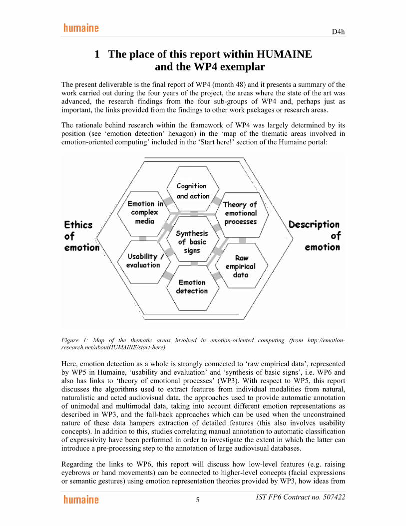
The rationale behind research within the framework of WP4 was largely determined by its position (see ‘emotion detection’ hexagon) in the ‘map of the thematic areas involved in emotion-oriented computing’ included in the ‘Start here!’ section of the Humaine portal:

Figure 1: Map of the thematic areas involved in emotion-oriented computing (from http://emotion-research.net/aboutHUMAINE/start-here)

Here, emotion detection as a whole is strongly connected to ‘raw empirical data’, represented by WP5 in Humaine, ‘usability and evaluation’ and ‘synthesis of basic signs’, i.e. WP6 and also has links to ‘theory of emotional processes’ (WP3). With respect to WP5, this report discusses the algorithms used to extract features from individual modalities from natural, naturalistic and acted audiovisual data, the approaches used to provide automatic annotation of unimodal and multimodal data, taking into account different emotion representations as described in WP3, and the fall-back approaches which can be used when the unconstrained nature of these data hampers extraction of detailed features (this also involves usability concepts). In addition to this, studies correlating manual annotation to automatic classification of expressivity have been performed in order to investigate the extent in which the latter can introduce a pre-processing step to the annotation of large audiovisual databases.

Regarding the links to WP6, this report will discuss how low-level features (e.g. raising eyebrows or hand movements) can be connected to higher-level concepts (facial expressions or semantic gestures) using emotion representation theories provided by WP3, how ideas from

D4h


image processing and scene analysis can be utilized in virtual environments, supplying ECAs with attention capabilities and how real-time feature extraction from facial expressions and hand gestures can be used to render feedback-capable ECAs.

This deliverable summarises work reported in past documents by:

S. Abrilian, V. Aharonson, N. Amir, E. Andre, S. Asteriadis, A. Batliner, G. Caridakis, A. Cerekovic, R. Cowie, L. Devillers, D. Grandjean, F. Hoenig, S. Ioannou, K. Karpouzis, L. Kessous, J. Kim, S. Kollias, L. Lamel, M. Mancini, JC. Martin, E. McMahon, I. Pandžić, C. Pelachaud, A. Raouzaiou, B. Schuller, L. Vidrascu, T. Vogt, G. Zorić

The corresponding institutions that have contributed in past reports are:

ICCS, DIST,FAU, FER, LIMSI/CNRS, Paris 8, QUB, TAU, TUM, UA, UNIGE

D4h


2 Brief Overview of Workpackage 4 and Its Exemplar

2.1 Introduction

The following table summarizes collaborative efforts in the framework of WP4. As mentioned in previous reports, work within the work package has followed two directions, unimodal (visual, aural and biosignal) processing and recognition and multimodal work; in addition to this, in order to move toward applying algorithms designed to work in controlled situations (‘lab environments’) in real-life data and tackling the requirements imposed by the latter, parts of the work focused on natural (e.g. emoTV, emoTaboo clips) or naturalistic (older SALAS clips) data, while other part investigated uni- or multimodal analysis and recognition in newly created datasets in studio-like environments (e.g. Genoa, GEMEP). As was expected, in the case of lab environment data, the widest selection of features was available, catering for better recognition rates and finer resolution of labels. In the case of natural and naturalistic data, clips belong to two categories, those captured from TV programmes, such as the emoTV dataset and some clips from the Humaine database, while others were recorded in good lighting conditions and showed constrained expressivity, while still inducing and showing real-life emotions (SALAS clips and similar clips from the Humaine database). As a result of this distinction, different features and labels with different scope were extracted in these cases.

Uni

mod

al CEICES

Humaine database EmoTV, EmoTaboo SALAS

Genoa

Mul

timod

al

EmoTaboo, SALAS Genoa, GEMEP

Natural – naturalistic Lab environment – acted

Table 1: Summary of analyzed datasets and characteristics

In the following, we will briefly discuss each sub-group and related research focus, before investigating the deployed algorithms and produced results (in the next chapter).

2.2 Sub-group 1: Speech analysis and recognition

Analysis and recognition of speech data (as well as induction and annotation performed within WP5) was mainly carried out around the CEICES [1] initiative. CEICES (Combining Efforts for Improving automatic Classification of Emotional user States) is a co-operation between several Humaine and non-Humaine sites, dealing with classification of emotional user states conveyed in German speech recordings of 51 ten- to thirteen-year old children communicating with Sony’s AIBO pet robot. This corpus, a parallel activity across WP4 and WP5, essentially contains spontaneous phrases from children interacting with a pet robot;

D4h


these were segmented in smaller chunks, analyzed and different sets of features were extracted and tested in terms of classification accuracy and efficiency. This part largely differentiates the approach followed in the speech sub-group from the one followed in the visual analysis subgroup, since the size of the possible feature set here is enormous, and since most features are based on transforming the raw signal, extracting confidence values on the features per se is not possible; as a result, feature selection and reduction of the feature set is a task far from trivial and automatic classification with different feature constellations can provide varying results and efficiency.

Feature extraction and classification has also been performed on the Genoa and GEMEP data sets, recorded in lab environments. Since segmentation of the clips is based on speech characteristics (i.e. tunes, where by definition each tune may contain only one emotion label), emotion recognition performs very well. This is also the case when processing the SALAS clips; the added value here was that the speech channel was also used to extract phonemes, which were in turn mapped to visemes and associated with visual features.

2.3 Sub-group 2: Visual analysis and recognition

The decision to treat natural or naturalistic videos in a different manner that those captured in a lab environment or those showing acted expressivity is noticeable in the algorithms deployed for visual analysis and the sets of extracted features.

In the early part of Humaine, visual analysis concentrated on working with existing naturalistic data, captured within the framework of the FP5 ERMIS [17] project. These data were among the first datasets to be induced, recorded, segmented, annotated and processed with naturalistic expressivity in mind; as a result, the task of providing robust feature extraction and classification mechanisms, as well as taking into account multimodality, was extremely challenging. In the following, the technical requirements of these videos also served as a guide for additional recordings in lab environments, showing acted expressivity: the Genoa and GEMEP [41] datasets, which illustrate facial expressivity, along with hand gesturing and expressive speech, illustrate the need to produce high-quality recordings, technologically-speaking, even if natural interaction or emotion induction is sacrificed in the process. This need arises from the fact that the interplay between different modalities (speech and video, or even within the visual modality itself with facial and hand expressivity) is still explored and remains an open research issue. This multimodal aspect of human expressivity has to be investigated, taking perhaps into account external information, such as personality or context, before taking the developed algorithms ‘to the wild’, i.e. in real-life circumstances, in terms of recording environments and expressivity. When it comes to such recordings, emoTV data, and its sister, emoTaboo dataset, were analyzed in terms of extracting visual features. Since video quality was far from perfect in the case of the emoTV dataset, it was not possible to extract detailed visual features; as a result, the emphasis was shifted towards detecting higher-level expressivity, based on features inspired from the Laban parameters, initially used to synthesize gestures in the framework of Humaine. Results from these clips show that it is possible to use this approach to identify expressive segments in long video footage and even separate active from passive scenes.

D4h


2.4 Sub-group 3: Analysis and recognition of physiological features

Analysis and recognition of physiological features is an area usually overlooked when dealing with affect recognition in natural settings, mainly due to the intrusive nature of the sensors used to capture the data and the ethical, as well as practical questions related to emotion induction.

For the most part of Humaine, related research has to do with improving and testing the Augsburg Biosignal Toolbox (AuBT) [26]. AuBT is written in Matlab and provides a graphical user interface which allows the user to extract features from common physiological signals, select relevant ones and use them to train and evaluate a classifier. It comes along with two data corpora containing physiological data of a single user recorded in different emotional states.

Within 2007, FAU Erlangen [15] collected a comprehensive multi-modal database of relaxed and stressed user states during a simulated car-drive, the Drivawork (Driving Under Varying Workload – [16]) database. Audio, video and six physiological signals, electrocardiogram (ECG), electromyogram at the neck (EMG), skin conductivity between index and middle finger (SC), skin temperature at the little finger (Temp), blood volume pulse at the ring finger (BVP) and abdominal respiration (Resp), were recorded. To collect the database, LCT (Lane Change Task), a PC-based tool to assess driver distraction requiring only standard consumer equipment was used, providing uniform driving demands and readily yielding measures of driving performance. During the test, the driver is given additional mental tasks, intending to elicit an increased stress level: a memory task, question answering and mental arithmetic. In addition to these, reading and question tasks in different contexts are used to elicit speech under different stress levels.

2.5 Sub-group 4: Multimodal recognition

In the framework of the work presented in Table 1 and in the previous reporting documents, the main task related to multimodal analysis was to test different combinations of modalities with different learning algorithms and evaluate their results. One of the main obstacles here was the difference in resolutions between the speech features (one set per tune, typically lasting up to 20-30 frames) and the visual features (one feature set per frame); the finer resolution of the visual signal catered for the better location of expressivity within a tune or a larger clip (e.g. emoTaboo) which, in turn, provided better definition of its position on the Feeltrace [35] place. In addition to this, the confidence values associated with the visual features enabled most approaches to drop feature sets with high uncertainty, thus improving the learning process.

Regarding unimodal performance, since the smallest unit for which recognition was attempted was a tune, which is defined as the segment between two pauses, i.e. is speech-related, prosody features performed better than visual features using the same, non-dynamic classifier. One of the important outcomes of the modalities integration process was that with the introduction of additional multimodal datasets (especially Genoa and GEMEP), even more approaches were tested, verifying the fact that multimodal analysis performs better than all unimodal approaches, even in the presence of uncertainty. An additional fact is that dynamic analysis (in our case, using recurrent neural nets) is able to capture expressivity even within the small span of a tune, while still retaining the ability to generalize, mostly for the same subject, but in a certain extent to other subjects as well.

D4h


In the latter case, an adaptation/retraining strategy was used in the SALAS dataset, using one subject for the initial training and testing and other subjects for testing and adaptation. Results show that the adaptation process is as affective as training from scratch on new subjects, in terms of classification, but for a large set of features such as the multimodal (face and prosody) one, is far superior in terms of training time. As a general rule, it does not make much sense to train different classifiers for different subjects; if the need to adapt is detected, a retraining step can improve classification in a much quicker fashion.

D4h


3 Advancing the state of the art

3.1 The CEICES initiative – results and findings

The approach followed within CEICES looks like this: the originator site provided speech files, phonetic lexicon, manually corrected word segmentation, emotional labels, definition of train and test samples, etc. Moreover, a balanced sub-sample was defined which contains roughly the same number of four different cover labels (Angry, Motherese, Emphatic, Neutral); initial experiments were performed only for this well-defined sub-sample, which contains 6070 words or 3996 turns respectively with manually corrected word segmentation. Annotation has been word-based, thus we aimed at two different classification tasks: word-based classification, and turn-based classification; for the latter, the word-based labels were converted into turn-based ones. Two-fold cross-classification to ensure strict speaker-independence was applied: the first school class as training set and the second school class as test set, and vice versa.

3.1.1 Trying different feature sets and classification approaches [1] describes a number of classification experiments conducted independently at each site as well as experiments using most important features from each site or class assignment with confidence scores within the ROVER approach (turn-based classification, two-fold cross-validation). Table 2 from the paper summarizes the independent experiments:

Table 2: Features and classifiers: per site, # of features before/after feature selection; # per type of features, and their domain; classifier used, weighted average recognition rate RR and non-weighted class-wise averaged recognition rate CL; used or not used (-) in ROVER and in classification with all features; SVM = Support Vector Machines.

Irrespective of the types of features and classifiers used, the results are roughly of the same order of magnitude; these figures are, for a 4-class problem and for realistic, spontaneous speech which does not only contain prototypical, very clear cases, in the expected range.

Our

heuristic threshold of 70% for the definition of MV cases, cf. above, may have resulted in lower classification performance than a threshold of 50%. However, we were not interested in manipulating the data to obtain the highest possible recognition rates, but rather in a realistic setting which takes into account possible applications. Best non-weighted class-wise average recognition rate CL combining 381 "most relevant" features from each site was 58.7% obtained with Random forests; regardless of the classifier chosen, each feature type contributed to optimal classification performance. Best CL using ROVER was 62.4%. As for details we refer to [1].

D4h


These results illustrate an initial range of performance for this task; they should not be conceived of as competing with each other. We found it hard to control all aspects of processing at the different sites which used, e.g. different feature normalization and selection procedures.

Our intention was that with this step, each site can reduce its own large feature set

(sometimes > 1000 features) to a smaller set with most of the relevant features.

3.1.2 The impact of erroneous F0 extraction [2] Traditionally, it has been assumed that pitch is the most important prosodic feature for the marking of prominence, and of other phenomena such as the marking of boundaries or emotions. This role has been put into question by recent studies. As nowadays larger databases are always being processed automatically, it is not clear up to what extent the possibly lower relevance of pitch can be attributed to extraction errors or to other factors. For the AMEN sub-corpus (4543 chunks, 613278 frames), the F0 values obtained by the ESPS pitch detection algorithm were corrected manually, yielding more than 6 % gross F0 errors in the voiced parts of the words. We compared the performance of the automatically extracted F0 values and of the manually corrected F0 values for the automatic recognition of prominence (2 classes: neutral vs. emphatic) and emotion (4 classes: motherese, neutral, emphatic, angry). The difference in classification performance between corrected and automatically extracted pitch features turns out to be consistent but not very pronounced. Thus it is likely that a lower relevance of pitch for emotion recognition is only partly due to extraction errors.

3.1.3 Laryngealizations (voice quality) and emotion [4] It has been claimed that voice quality traits including irregular phonation such as creaky voice (laryngealization) serve several functions, amongst them being the marking of emotions; accordingly, they should be used for automatic recognition of these phenomena. However, laryngealizations marking emotional states have mostly been found for acted or synthesized data. First results using real-life data do not corroborate such an impact of laryngealized speech for the marking of emotions. For our AMEN sub-corpus, we operationalized the F0 extraction errors described above as indications of laryngealized passages. Even if at first sight, it seems plausible that some emotions might display higher frequencies of laryngealizations, at a closer look, we find that it is rather a combination of speaker-specific traits and lexical/segmental characteristics which causes the specific distribution. We argue that the multi-functionality of phenomena such as voice quality traits makes it rather difficult to transfer results from acted/synthesized data onto realistic speech data, and especially, to employ them for speaker-independent automatic processing, as long as very large databases modelling diversity to a much higher extent are not available.

3.1.4 The impact of feature type and functionals on classification performance [9]

We pooled together a total of 4244 features extracted at all sites taking part in the CEICES initiative and grouped them into 12 low level descriptor types and 6 functional types, based on the above mentioned feature encoding scheme. For each of these groups, classification results using Support Vector Machines and Random Forests were computed for the full set of features, and for 150 features each with the highest individual Information Gain Ratio. The performance for the different groups varies mostly between approx. 50 % and approx. 60 %. For the acoustic types, results were between 50.6 % (voice quality) and 60.1 % (duration); for the linguistic types, best results are achieved with bag of words (62.8 %) but even with only 6 part-of-speech classes, 54.9 % could be obtained.

D4h


3.1.5 Emotion recognition with reverberated and noisy speech [8] The Aibo corpus is available with good microphone quality (close-talk microphone), as artificially reverberated speech, and with low microphone quality (room microphone). It is well known that speech recognition normally deteriorates if faced with low quality speech, but we do not know of comparable studies on the performance of emotion recognition using low quality speech. We compared three different data-sets: the Berlin Emotional Speech Database, the Danish Emotional Speech Database, and the AMEN sub-corpus. By using different feature types such as word- or turn-based statistics, manual versus forced alignment, and optimization techniques we show how to best cope with this demanding task and how noise addition or different microphone positions affect emotion recognition. It turned out that emotion recognition seems to be less prone to noise than other speech processing tasks.

3.2 Real-time/detailed facial feature extraction

In the field of facial feature extraction, two approaches were followed: initially, improving on the work started within the ERMIS project [17], the emphasis was put on detecting prominent feature points with the highest possible degree of robustness and accuracy, in order to assist facial expression recognition from the SALAS video clips. A multi-cue approach, where colour, edge and hue information were taken into account, also produced a confidence value associated with the extracted features, catering for their dismissal in cases of uncertainty or otherwise taking into account low confidence scores. In 2007, a parallel activity concentrating on the speed of feature extraction, rather than high accuracy, was pursued to allow for real-time applications. While the latter is not robust enough to cater for high percentages in recognition, it has been extremely useful in interactive applications, providing also non-verbal info such as gaze and pose direction.

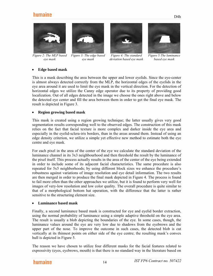
3.2.1 Multi-cue facial feature extraction A wide variety of methodologies have been proposed in the literature for the extraction of different facial characteristics and especially for the eyes, in both controlled and uncontrolled environments. What is common among them is that, regardless of the overall success rate that they have, they all fail in some set of cases, due to the inherent difficulties and external problems that are associated with the task. As a result, it is not reasonable to select a single methodology and expect it to work optimally in all cases. In order to overcome this, in this work we choose to utilize multiple different techniques in order to locate the most difficult facial features, i.e. the eyes and the mouth.

• MLP based mask

This approach refines eye locations extracted by an MLP (Multi-layer perceptron) network. It builds on the fact that eyelids usually appear darker than skin due to eyelashes and are almost always adjacent to the iris. Thus, by including dark objects near the eye centre, we add the eyelashes and the iris in the eye mask. The result is depicted in Figure 2.

D4h


Figure 2: The MLP based

eye mask Figure 3: The edge based

eye mask

Figure 4: The standard deviation based eye mask

Figure 5:The luminance based eye mask

• Edge based mask

This is a mask describing the area between the upper and lower eyelids. Since the eye-center is almost always detected correctly from the MLP, the horizontal edges of the eyelids in the eye area around it are used to limit the eye mask in the vertical direction. For the detection of horizontal edges we utilize the Canny edge operator due to its property of providing good localization. Out of all edges detected in the image we choose the ones right above and below the detected eye center and fill the area between them in order to get the final eye mask. The result is depicted in Figure 3.

• Region growing based mask

This mask is created using a region growing technique; the latter usually gives very good segmentation results corresponding well to the observed edges. The construction of this mask relies on the fact that facial texture is more complex and darker inside the eye area and especially in the eyelid-sclera-iris borders, than in the areas around them. Instead of using an edge density criterion, we utilize a simple yet effective new method to estimate both the eye centre and eye mask.

For each pixel in the area of the center of the eye we calculate the standard deviation of the luminance channel in its 3x3 neighbourhood and then threshold the result by the luminance of the pixel itself. This process actually results in the area of the center of the eye being extended in order to include some of its adjacent facial characteristics. The same procedure is also repeated for 5x5 neighborhoods; by using different block sizes we enhance the procedure’s robustness against variations of image resolution and eye detail information. The two results are then merged in order to produce the final mask depicted in Figure 4. The process is found to fail more often than the other approaches we utilize, but it is found to perform very well for images of very-low resolution and low color quality. The overall procedure is quite similar to that of a morphological bottom hat operation, with the difference that the latter is rather sensitive to the structuring element size.

• Luminance based mask

Finally, a second luminance based mask is constructed for eye and eyelid border extraction, using the normal probability of luminance using a simple adaptive threshold on the eye area. The result is usually a blob depicting the boundaries of the eye. In some cases, though, the luminance values around the eye are very low due to shadows from the eyebrows and the upper part of the nose. To improve the outcome in such cases, the detected blob is cut vertically at its thinnest points on either side of the eye centre; the resulting mask’s convex hull is depicted in Figure 5.

The reason we have chosen to utilize four different masks for the facial features related to expressivity (eyes, eyebrows, mouth) is that there is no standard way in the literature based on

D4h


which to select the ideal eye localization methodology for a given facial image. Consequently, it is not easy to judge which one of the four detected masks is the best performing and select it as the output of the overall eye localization module. Instead, we choose to combine the different masks using a committee machine.

• Mask fusion

Given the fact that each one of the different methodologies that we have utilized has some known strong and weak points, the committee machine that is most suitable for the task of mask fusion is the mixture of experts dynamic structure, properly modified to match our application requirements [37]. The general structure of this methodology is presented in Figure 6. It consists of k supervised modules (the experts) and a gating network that performs the function of a mediator among the experts. The main assumption is that each one of the experts operates best in different regions of the input space in accordance with a probabilistic model that is known a priori, hence the need of the gating network.

Figure 6: ‘Mixture of experts’ architecture

The role of the gating network is to estimate, based on the input, the probability ig that each individual expert i operates correctly, and to provide these estimations to the output combiner module. The gating network consists of a single layer of softmax neurons; the choice of softmax as the activation function for the neurons has the important properties of

kigi ..1,10 ∈∀≤≤ , 11

=∑=

k

iig

i.e. it allows for the estimations to be interpreted as probabilities. In our work we have 4=k experts; the implementations of the eye detection methodologies presented earlier in the

section. The gating network favors the color based feature extraction methods in images of high color and resolution, thus incorporating the a priori known probabilities of success for our experts in the fusion process.

Additionally, the output combiner module which normally operates as egy ⋅= , where e is the vector of expert estimations, is modified in our work to operate as

fefgy ⋅⋅

=

D4h


where f is the vector of confidence values associated with the output of each expert, thus further enhancing the quality of the mask fusion procedure. Confidence values are computed by comparing the location, shape and size of the detected masks to those acquired from anthropometric statistical studies.

The modified combiner module fuses the four masks together by making pixel by pixel decisions. The result of the procedure for the left eye in a frame of the SALAS dataset is depicted in Figure 7.

Figure 7: The final mask for the left eye

3.2.2 Real time feature extraction – estimation of head pose and eye gaze

• Real time feature extraction

In this work, prior to eye and mouth region detection, face detection is applied on the face images. The face is detected using the Boosted Cascade method, described in [34]. The output of this method is usually the face region with some background. Furthermore, the position of the face is often not centered in the detected sub-image. Since the detection of the eyes and mouth will be done on blocks of a predefined size, it is very important to have an accurate face detection algorithm. Consequently, a technique to postprocess the results of the face detector is used.

More specifically, a technique that compares the shape of a face with that of an ellipse is used. This technique is based on the work reported in [32]. According to this, the distance map of the face area found at the first step is extracted. Here, the distance map is calculated from the binary edge map of the area. An ellipsis scans the distance map and a score that is the average of all distance map values on the ellipse contour el, is evaluated.

( , )

1( , )

x y el

score D x yel ∈

= ∑

where D is the distance map of the region found by the Boosted Cascade algorithm. This score is calculated for various scale and shape transformations of the ellipses. The transformation which gives the best score is considered as the one that corresponds to the ellipses that best describes the exact face contour. The lateral boundaries of the ellipses are the new boundaries of the face region.

A template matching technique follows for the facial feature area detection step: The face region found by the face detection step is brought to certain dimensions and the corresponding Canny edge map is extracted. Subsequently, for each pixel on the edge map, a vector pointing to the closest edge is calculated and its x,y coordinates are stored. The final result is a vector field encoding the geometry of the face. Prototype eye patches were used for the calculation of their corresponding vector fields and the mean vector field was used as prototype for

D4h


searching similar vector fields on areas of specified dimensions on the face vector field. The similarity between an image region and the templates is based on the following distance measure:

2|| ||

k

L i ii R

E v m∈

= −∑

where || || denotes the L2 norm. Essentially for a NxM region Rk the previous formula is the sum of the euclidean distances between vectors vi of the candidate region and the corresponding mi of the mean vector field (template) of the eye we are searching for (right or left). The candidate region on the face that minimizes EL2 is marked as the region of the left or right eye. To make the algorithm faster we utilize the knowledge of the approximate positions of eyes on a face.

For the eye center detection, the normalized area of the eye is brought back to its initial dimensions on the image and a light reflection removal step is employed. The grayscale image of the eye area is converted to a binary image and small white connected components are removed. The areas that correspond to such components on the original image are substituted by the average of their surrounding area. The final result is an eye area having reflections removed. Subsequently, horizontal and vertical derivative maps are extracted from the resulting image and they are projected on the vertical and horizontal axis respectively. The mean of a set of the largest projections is used for an estimate of the eye center. Following, a small window around the detected point is used for the darkest patch to be detected, and its center is considered as the refined position of the eye center.

For the detection of the eye corners (left, right, upper and lower) a technique similar to that described in [39] is used: Having found the eye center, a small area around it is used for the rest of the points to be detected. This is done by using the Generalized Projection Functions (GPFs) which are a combination of the Integral Projection Functions (IPFs) and the Variance Projection Functions (VPFs). The integral projection function’s value on row (column) x (y) is the mean of its luminance intensity, while the Variance Projection Function on row x is its mean variance. The GPF’s value on a row (column) x (y) is a linear combination of the corresponding values of the derivatives of the IPF and VPF on row x (column y):

' '( ) (1 ) ( )u u uGPF x a IPF x a VPF= − ∗ + ∗ , ' '( ) (1 ) ( )v v vGPF y a IPF y a VPF= − ∗ + ∗

Local maxima of the above functions are used to declare the positions of the eye boundaries.

For the mouth area localization, a similar approach to that of the eye area localization is used: The vector field of the face is used and template images are used for the extraction of a prototype vector field of the mouth area. Subsequently, similar vector fields are searched for on the lower part of the normalized face image. However, as the mouth has, many times, similar luminance values with its surrounding skin, an extra factor is also taken into account. That is, at every search area, the mean value of the hue component is calculated and added to the inverse distance from the mean vector fields of the mouth. Minimum values declare mouth existence.

For the extraction of the mouth points of interest (mouth corners), the hue component is also used. Based on the hue values of the mouth, the detected mouth area is binarized and small connected components whose value is close to 0o are discarded similar to the light reflection removal technique employed for the eyes. The remainder is the largest connected component

D4h


which is considered as the mouth area. The leftmost and rightmost points of this area are considered as the mouth corners. An example of detected feature points is shown in Figure 8.

Once the positions of the facial feature points of interest are known on a frontal face, tracking can follow. In this way, gaze detection and pose estimation can be determined, not only on a single frame, but on a series of frames. Also, calculating changes of the interocular distance in a series of frames, it is easy to determine the distance of a user from the camera. Furthermore, tracking saves computational time, since detecting the characteristics at every frame is more time demanding, and can achieve better results in cases of large displacement of the face from its frontal position. In our case, tracking was done using an iterative, 3-pyramid Lucas-Kanade tracker [28]. An example of a person’s movement with relation to the camera is shown in Figure 9.

Figure 8: Detected facial features Figure 9: Estimation of movement towards the camera

• Head pose and eye gaze

In recent bibliography, most gaze detection and pose determination techniques need special hardware setup. Examples of such cases are the work described in [27], where a large resolution image of the iris is necessary and the work in [40], where a specific architecture has to be followed. In other cases, intrusive devices have to be worn by the user [10], making the system less appropriate for wide-range applications.

In the current work [36], features are detected and tracked, allowing for a relative freedom of the user, under good lighting conditions. Under these circumstances, the gaze directionality can be approximately determined, which is enough for attention recognition purposes, as well as for general decisions regarding the user’s gaze. For gaze detection, the area defined by the four points around the eye is used. Eye areas depicting right, left, upper and lower gaze directionalities are used to calculate mean grayscale images corresponding to each gaze direction. The areas defined by the four detected points around the eyes, are then correlated to these images. The normalized differences of the correlation values of the eye area with the left and right as well as upper and lower mean gaze images are calculated:

, ,

, , , ,

, ,

, , , ,

, ,

, , , ,

, ,

, , , ,

( )max( , , , )

( )max( , , , )

( )max( , , , )

max( , , , )

r l r rr

r l r r r u r d

r u r dr

r l r r r u r d

l l l rl

l l l r l u l d

l u l dl

l l l r l u l d

R RH

R R R RR R

VR R R R

R RH

R R R RR R

VR R R R

−=

−=

−=

−=

D4h


Where Ri,j is the correlation of the i (i=left,right) eye with the j (j=left, right, upper, lower) mean grayscale image. The normalized value of the horizontal and vertical gaze directionalities (conventionally, angles) are then the weighted mean:

((2 ) ) / 2((2 ) ) / 2

r l

r l

H l H l HV l V l V

= − ⋅ + ⋅= − ⋅ + ⋅

Where l is the fraction of the mean intensity in the left and right areas. This fraction is used to weight the gaze directionality values so that eye areas of greater luminance are favored in cases of shadowed faces.

To estimate the pose of a face based on the features detected, orthographic projection can be assumed for a linear system to be constructed, since depth information is not necessary for pose estimation. The pose of the face is a problem of estimating the direction of the face-plane which depends on the changes of the distances between facial characteristics. Thus, if the eye and mouth centers are considered, it is possible to initialize a triangle A, B, C, with A, B being the left and right eye centers and C the mouth center at the frontal view. Let A’, B’ and C’ be the displaced positions of these points, which are considered to be known since the points are tracked. The α, β, γ rotation angles around the y, z, x-axis are [5]:

'

'

'

arcsin

arccoscos

arccoscos

x

y

x

x

y

y

CC

AA

CC

γ

βγ

αγ

=

=

=

3.3 Dynamic recognition of naturalistic affective states

In order to consider the dynamics of displayed expressions we need to utilize a classification model that is able to model and learn dynamics, such as a Hidden Markov Model or a recursive neural network In this work we are using a recursive neural network; see Figure 10. This type of network differs from conventional feed-forward networks in that the first layer has a recurrent connection. The delay in this connection stores values from the previous time step which can be used in the current time step, thus providing the element of memory.

x1w

1b 2b

2w 1a

1ar2ax 1a 2a

Figure 10: The recursive neural network

D4h


Although we are following an approach that only comprises a single layer of recurrent connections, in reality the network has the ability to learn patterns of a greater length as well, as current values are affected by all previous values and not only by the last one.

Out of all possible recurrent implementations we have chosen the Elman net for our work [14]. This is a two-layer network with feedback from the first layer output to the first layer input. This recurrent connection allows the Elman network to both detect and generate time-varying patterns.

The transfer functions of the neurons used in the Elman net are tan-sigmoid for the hidden (recurrent) layer and purely linear for the output layer. More formally

1-e12)(tan 12-

11

ikii ksiga+

== and 22jj ka =

where 1ia is the activation of the i-th neuron in the first (hidden) layer, 1

ik is the induced local field or activation potential of the i-th neuron in the first layer, 2

ja is the activation of the j-th

neuron in the second (output) layer and 2jk is the induced local field or activation potential of

the j-th neuron in the second layer.

The input layer of the utilized network has 57 neurons (25 for the FAPs and 32 for the audio features). The hidden layer has 20 neurons and the output layer has 5 neurons, one for each one of five possible classes: Neutral, Q1 (first quadrant of the Feeltrace [35] plane), Q2, Q3 and Q4. The network is trained to produce a level of 1 at the output that corresponds to the quadrant of the examined tune and levels of 0 at the other outputs.

3.3.1 Classification The most common applications of recurrent neural networks include complex tasks such as modeling, approximating, generating and predicting dynamic sequences of known or unknown statistical characteristics. In contrast to simpler neural network structures, using them for the seemingly easier task of input classification is not equally simple or straight forward.

The reason is that where simple neural networks provide one response in the form of a value or vector of values at their output after considering a given input, recurrent neural networks provide such inputs after each different time step. So, one question to answer is at which time step the network’s output should be read for the best classification decision to be reached.

As a general rule of thumb, the very first outputs of a recurrent neural network are not very reliable. The reason is that a recurrent neural network is typically trained to pick up the dynamics that exist in sequential data and therefore needs to see an adequate length of the data in order to be able to detect and classify these dynamics. On the other hand, it is not always safe to utilize the output of the very last time step as the classification result of the network because:

1. the duration of the input data may be a few time steps longer than the duration of the dominating dynamic behavior and thus the operation of the network during the last time steps may be random

2. a temporary error may occur at any time step of the operation of the network

D4h


For example, in Figure 11 we present the output levels of the network after each frame when processing the tune of the running example. We can see that during the first frames the output of the network is quite random and changes swiftly. When enough length of the sequence has been seen by the network so that the dynamics can be picked up, the outputs start to converge to their final values. But even then small changes to the output levels can be observed between consecutive frames.

00,10,20,30,40,50,60,70,80,9

1

0 5 10 15 20 25

NeutralQ1Q2Q3Q4

-0,3

-0,2

-0,1

0

0,1

0,2

0,3

0,4

0,5

0,6

0 5 10 15 20 25

Figure 11: Individual network outputs after each frame Figure 12: Margin between correct and next best

output

Although these are not enough to change the classification decision (see Figure 12) for this example where the classification to Q1 is clear, there are cases in which the classification margin is smaller and these changes also lead to temporary classification decision changes.

x1w

1b 2b

2w 1a

1ar

Input Layer

Hidden Layer Output Layer Integrating Module

ox 1a 2a o( )c−1 o

c 2a

Figure 13. The Elman net with the output integrator

In order to arm our classification model with robustness we have added a weighting integrating module to the output of the neural network which increases its stability (see Figure 13). Specifically, the final outputs of the model are computed as:

( ) ( ) ( )112 −⋅−+⋅= tocacto jjj

where ( )to j is the value computed for the j-th output after time step t, ( )1−to j is the output value computed at the previous time step and c is a parameter taken from the (0,1] range that controls the sensitivity/stability of the classification model. When c is closer to zero the model becomes very stable and a large sequence of changed values of 2

jk is required to affect the classification results while as c approaches one the model becomes more sensitive to changes in the output of the network. When 1=c the integrating module is disabled and the network output is acquired as overall classification result. In our work, after observing the models performance for different values of c , we have chosen 5.0=c .

D4h


Of course, in order for this weighted integrator to operate, we need to define output values for the network for time step 0, i.e. before the first frame. It is easy to see that due to the way that the effect of previous outputs wares off as time steps elapse due to c , this initialization is practically indifferent for tunes of adequate length. On the other hand, this value may have an important affect on tunes that are very short. In this work, we have chosen to initialize all initial outputs at ( ) 00 =o .

3.3.2 Results and comparison From the application of the proposed methodology on the data set annotated as ground truth we acquire a measurement of 81,55% for the system’s accuracy. Specifically, 389 tunes were classified correctly, while 88 were misclassified. Clearly, this kind of information, although indicative, is not sufficient to fully comprehend and assess the performance of our methodology.

Towards this end, we provide in Table 3 the confusion matrix for the experiment. In the table rows correspond to the ground truth and columns to the system’s response. Thus, for example, there were 5 tunes that were labeled as neutral in the ground truth but were misclassified as belonging to Q2 by our system.

Neutral Q1 Q2 Q3 Q4 Totals

Neutral 34 1 5 3 0 43 Q1 1 189 9 12 6 217 Q2 4 3 65 2 1 75 Q3 4 6 7 39 3 59 Q4 4 6 4 7 62 83

Totals 47 205 90 63 72 477

Table 3. Overall confusion matrix

Still, in our analysis of the experimental results so far we have not taken into consideration a very important factor: that of the length of the tunes. In order for the Elman net to pick up the expression dynamics of the tune an adequate number of frames needs to be available as input. Still, there is a number of tunes in the ground truth that are too short for the network to reach a point where its output can be read with high confidence.

In order to see how this may have influence our results we present in the following separate confusion matrices for short (see Table 6 and Table 7) and normal length tunes (see Table 4 and Table 5). In this context we consider as normal tunes that comprise at least ten (i.e. less than half a second) frames and as short tunes with length from one up to nine frames.

First of all, we can see right away that the performance of the system, as was expected is quite different in these two cases. Specifically, there are 83 errors in just 131 short tunes while there are only 5 errors in 346 normal tunes. Moreover, there are no severe errors in the case of long tunes, i.e. there are no cases in which a tune is classified in the exact opposite quadrant than in the ground truth.

Overall, the operation of our system in normal operating conditions (as such we consider the case in which tunes have a length of at least 10 frames) is accompanied by a classification rate of 98,55%, which is certainly very high, even for controlled data, let alone for naturalistic data.

D4h



Neutral 29 0 0 0 0 29 Q1 0 172 3 0 0 175 Q2 1 1 54 0 0 56 Q3 0 0 0 30 0 30 Q4 0 0 0 0 56 56

Totals 30 173 57 30 56 346

Table 4. Confusion matrix for normal tunes

Neutral Q1 Q2 Q3 Q4 Totals Neutral 100,00% 0,00% 0,00% 0,00% 0,00% 100,00%

Q1 0,00% 98,29% 1,71% 0,00% 0,00% 100,00% Q2 1,79% 1,79% 96,43% 0,00% 0,00% 100,00% Q3 0,00% 0,00% 0,00% 100,00% 0,00% 100,00% Q4 0,00% 0,00% 0,00% 0,00% 100,00% 100,00%

Totals 8,67% 50,00% 16,47% 8,67% 16,18% 100,00%

Table 5. Confusion matrix for normal tunes expressed in percentages

Of course, the question still remains of whether it is meaningful for the system to fail so much in the case of the short tunes, or if the information contained in them is sufficient for a considerably better performance and the system needs to be improved. In order to answer this question we will use Williams’ index [19].

This index was originally designed to measure the joint agreement of several raters with another rater. Specifically, the index aims to answer the question: “Given a set of raters and one other rater, does the isolated rater agree with the set of raters as often as a member of that set agrees with another member in that set?” which makes it ideal for our application.

In our context, the examined rater is the proposed system. In order to have an adequate number of raters for the application of Williams’ methodology we have asked three additional humans to manually classify the 131 short tunes into one of the five considered emotional categories. In our case, Williams’ index for the system with respect to the four human annotators is reduced to the following:

The joint agreement between the reference annotators is defined as:

( ) ( )∑ ∑= +=−

=3

1

4

1,

1442

a abg baPP

where ( )baP , is the proportion of observed agreements between annotators a and b

( ) ( ) ( ){ }131

:,

sRsRSsbaP ba =∈=

In the above S is the set of the 131 annotated tunes and ( )sRa is the classification that annotator a gave for tune s . The observed overall group agreement of the system with the reference set of annotators is measured by

( )

4

,04

10

∑== a

aPP

D4h


where we use 0 to denote the examined annotator, i.e. our system. Williams’ index for the system is the ratio:

gPPI 0

0 =

The value of 0I can be interpreted as follows: Let a tune be selected at random and rated by a randomly selected reference annotator. This rating would agree with the system’s rating at a

rate 100

0I percent of the rate that would be obtained by a second randomly selected reference

annotator. Applying this methodology for the 131 short tunes in the ground truth data set with reference to the one original and 3 additional human annotators we have calculated 12,10 =I . A rate of 0I that is larger than one, as we have computed in our example, indicates that the system agrees with the human annotators more often than they agree with each other. As our system does not disagree with the human annotators more than they disagree with each other, we can conclude that the system performs at least as well as humans do in the difficult and uncertain task of classifying so short tunes. Consequently, the poor classification performance of the system in the case of short tunes is fully understandable and should not be taken as an indication of a systematic failure or weakness.


Neutral 5 1 5 3 0 14 Q1 1 17 6 12 6 42 Q2 3 2 11 2 1 19 Q3 4 6 7 9 3 29 Q4 4 6 4 7 6 27

Totals 17 32 33 33 16 131

Table 6. Confusion matrix for short tunes

Neutral Q1 Q2 Q3 Q4 Totals Neutral 35,71% 7,14% 35,71% 21,43% 0,00% 100,00%

Q1 2,38% 40,48% 14,29% 28,57% 14,29% 100,00% Q2 15,79% 10,53% 57,89% 10,53% 5,26% 100,00% Q3 13,79% 20,69% 24,14% 31,03% 10,34% 100,00% Q4 14,81% 22,22% 14,81% 25,93% 22,22% 100,00%

Totals 12,98% 24,43% 25,19% 25,19% 12,21% 100,00%

Table 7. Confusion matrix for short tunes expressed in percentages

• Quantitative comparative study

In a previous work we have proposed a different methodology to process naturalistic data with the goal of estimating the human’s emotional state [38]. In that work a very similar approach is followed in the analysis of the visual component of the video with the aim of locating facial features. FAP values are then fed into a rule based system which provides a response concerning the human’s emotional state. In a later version of this work, we evaluate the likelihood of the detected regions being indeed the desired facial features with the help of anthropometric statistics acquired from [25] and produce degrees of confidence which are associated with the FAPs; the rule evaluation model is also altered and equipped with the

D4h


ability to consider confidence degrees associated with each FAP in order to minimize the propagation of feature extraction errors in the overall result [30].

When compared to our current work, these systems have the extra advantages of 1. considering expert knowledge in the form of rules in the classification process 2. being able to cope with feature detection deficiencies and.

On the other hand, they are lacking in the sense that 3. they do not consider the dynamics of the displayed expression and 4. they do not consider other modalities besides the visual one.

Thus, they make excellent candidates to compare our current work against in order to evaluate the practical gain from the proposed dynamic and multimodal approach. In Table 8 we present the results from the two former and the current approach. Since dynamics are not considered, each frame is treated independently in the preexisting systems. Therefore, statistics are calculated by estimating the number of correctly classified frames; each frame is considered to belong to the same quadrant as the whole tune.

It is worth mentioning that the results are from the parts of the data set that were selected as expressive for each methodology. But, whilst for the current work this refers to 72,54% of the data set and the selection criterion is the length of the tune, in the previous works only about 20% of the frames was selected with a criterion of the clarity with which the expression is observed, since frames close to the beginning or the end of the tune are often too close to neutral to provide meaningful visual input to a system. The performance of all approaches on the complete data set is presented in Table 9, where it is obvious that the dynamic and multimodal approach is by far superior.

Methodology Rule based Possibilistic rule based Dynamic and multimodal Classification rate 78,4% 65,1% 98,55%

Table 8. Classification rates on parts of the naturalistic data set

Methodology Rule based Possibilistic rule based Dynamic and multimodal Classification rate 27,8% 38,5% 98,55%

Table 9. Classification rates on the naturalistic data set

• Qualitative comparative study

As we have already mentioned, during the recent years we have seen a very large number of publications in the field of the estimation of human expression and/or emotion. Although the vast majority of these works is focused on the six universal expressions and use sequences where extreme expressions are posed by actors, it would be an omission if not even a qualitative comparison was made to the broader state of the art.

In Table 10 we present the classification rates reported in some of the most promising and well known works in the current state of the art. Certainly, it is not possible or fair to compare numbers directly, since they come from the application on different data sets. Still, it is possible to make qualitative comparisons base on the following information:

1. The Cohen2003 is a database collected of subjects that were instructed to display facial expressions corresponding to the six types of emotions. In the Cohn–Kanade database subjects were instructed by an experimenter to perform a series of 23 facial displays that included single action units and combinations of action units.

D4h


2. In the MMI database subjects were asked to display 79 series of expressions that included either a single AU or a combination of a minimal number of AUs or a prototypic combination of AUs (such as in expressions of emotion). They were instructed by an expert (a FACS coder) on how to display the required facial expressions, and they were asked to include a short neutral state at the beginning and at the end of each expression. The subjects were asked to display the required expressions while minimizing out-of-plane head motions.

3. In the Chen2000 subjects were asked to display 11 different affect expressions. Every emotion expression sequence lasts from 2s to 6s with the average length of expression sequences being 4s; even the shortest sequences in this dataset are by far longer than the short tunes in the SAL database.

4. The original instruction given to the actors has been taken as the actual displayed expression in all abovementioned databases, which means that there is an underlying assumption is that there is no difference between natural and acted expression.

As we can see, what is common among the datasets most commonly used in the literature for the evaluation of facial expression and/or emotion recognition is that expressions are solicited and acted. As a result, they are generally displayed clearly and to their extremes. In the case of natural human interaction, on the other hand, expressions are typically more subtle and often different expressions are mixed. Also, the element of speech adds an important degree of deformation to facial features which is not associated with the displayed expression and can be misleading for an automated expression analysis system.

Consequently, we can argue that the fact that the performance of the proposed methodology when applied to a naturalistic dataset is comparable to the performance of other works in the state of the art when applied to acted sequences is an indication of its success. Additionally, we can observe that when extremely short tunes are removed from the data set the classification performance of the proposed approach exceeds 98%, which, in current standards, is very high for an emotion recognition system.

The Multistream Hidden Markov Model approach is probably the one that is most directly comparable to the work presented herein. This is the alternative dynamic multimodal approach, where HMMs are used instead of RNNs for the modeling of the dynamics of expressions. Although a different data set has been utilized for the experimental evaluation of the MHMMs approach, the large margin between the performance rates of the two approaches indicates that the utilization of RNNs for dynamic multimodal classification of human emotion is a promising direction. Table 10. Classification rates reported in the broader state of the art [21], [29], [43]

Methodology Classification rate Data set TAN 83,31% Cohen2003

Multi-level HMM 82,46% Cohen2003 TAN 73,22% Cohn–Kanade

PanticPatras2006 86,6% MMIMultistream HMM 72,42% Chen2000

Proposed methodology 81,55% SAL Database Proposed methodology 98,55% Normal section of the SAL database

D4h


3.4 Multimodal adaptation and retraining

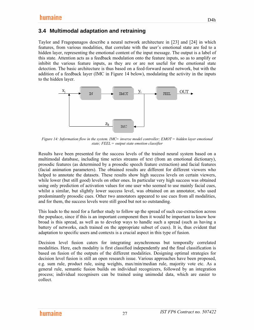
Taylor and Fragopanagos describe a neural network architecture in [23] and [24] in which features, from various modalities, that correlate with the user’s emotional state are fed to a hidden layer, representing the emotional content of the input message. The output is a label of this state. Attention acts as a feedback modulation onto the feature inputs, so as to amplify or inhibit the various feature inputs, as they are or are not useful for the emotional state detection. The basic architecture is thus based on a feed-forward neural network, but with the addition of a feedback layer (IMC in Figure 14 below), modulating the activity in the inputs to the hidden layer.

Figure 14: Information flow in the system. IMC= inverse model controller; EMOT = hidden layer emotional

state; FEEL = output state emotion classifier

Results have been presented for the success levels of the trained neural system based on a multimodal database, including time series streams of text (from an emotional dictionary), prosodic features (as determined by a prosodic speech feature extraction) and facial features (facial animation parameters). The obtained results are different for different viewers who helped to annotate the datasets. These results show high success levels on certain viewers, while lower (but still good) levels on other ones. In particular very high success was obtained using only prediction of activation values for one user who seemed to use mainly facial cues, whilst a similar, but slightly lower success level, was obtained on an annotator, who used predominantly prosodic cues. Other two annotators appeared to use cues from all modalities, and for them, the success levels were still good but not so outstanding.

This leads to the need for a further study to follow up the spread of such cue-extraction across the populace, since if this is an important component then it would be important to know how broad is this spread, as well as to develop ways to handle such a spread (such as having a battery of networks, each trained on the appropriate subset of cues). It is, thus evident that adaptation to specific users and contexts is a crucial aspect in this type of fusion.

Decision level fusion caters for integrating asynchronous but temporally correlated modalities. Here, each modality is first classified independently and the final classification is based on fusion of the outputs of the different modalities. Designing optimal strategies for decision level fusion is still an open research issue. Various approaches have been proposed, e.g. sum rule, product rule, using weights, max/min/median rule, majority vote etc. As a general rule, semantic fusion builds on individual recognizers, followed by an integration process; individual recognisers can be trained using unimodal data, which are easier to collect.

D4h


3.4.1 An adaptive neural network architecture Let us assume that we seek to classify, to one of, say, p available emotion classes ω, each input vector xi containing the features extracted from the input signal. A neural network produces a p-dimensional output vector )( ixy

[ ]Tiii

i ppppxy ωωω ...)(

21=

(1)

where ij

pω denotes the probability that the i-th input belongs to the j-th class.

Let us first consider that the neural network has been initially trained to perform the classification task using a specific training set, say, ( ) ( ){ }

bb mmb dxdxS ′′′′= ,,,, 11 L , where vectors ix′ and id ′ with bmi ,,2,1 L= denote the ith input training vector and the corresponding desired output vector consisting of p elements.

Then, let )( ixy denote the network output when applied to a new set of inputs, and let us consider the ith input outside the training set, possibly corresponding to a new user, or to a change of the environmental conditions. Based on the above described discussion, slightly different network weights should probably be estimated in such cases, through a network adaptation procedure.

Let bw include all weights of the network before adaptation, and aw the new weight vector which is obtained after adaptation is performed. To perform the adaptation, a training set Sc has to be extracted from the current operational situation composed of, (one or more), say, mc inputs; ( ) ( ){ }

cc mmc dxdxS ,,,, 11 L= where ix and id with cmi ,,2,1 L= similarly correspond to the ith input and desired output data used for adaptation. The adaptation algorithm that is activated, whenever such a need is detected, computes the new network weights aw , minimizing the following error criteria with respect to weights,

afaca EEE ,, η+= , ∑=

−=cm

iiiaac dxzE

1 2, )(21

, ∑=

′−′=bm

iiiaaf dxzE

12, )(

21

(2)

where acE , is the error performed over training set cS (“current” knowledge), afE , the corresponding error over training set bS (“former” knowledge); )( ia xz and )( ia xz ′ are the outputs of the adapted network, corresponding to input vectors ix and ix′ respectively, of the network consisting of weights aw . Similarly )( ib xz would represent the output of the network, consisting of weights bw , when accepting vector ix at its input; when adapting the network for the first time )( ib xz is identical to )( ixy . Parameter η is a weighting factor accounting for the significance of the current training set compared to the former one and 2⋅ denotes the L2 -norm.

The goal of the training procedure is to minimize (2) and estimate the new network weights wa , i.e., 0

aW and aw respectively [31]. Let us first assume that a small perturbation of the network weights (before adaptation) wb is enough to achieve good classification performance. Then,

a bw w w= + Δ (3)

D4h


Where wΔ are small increments. This assumption leads to an analytical and tractable solution for estimating aw , since it permits linearization of the non-linear activation function of the neuron, using a first order Taylor series expansion.

Equation (2) indicates that the new network weights are estimated taking into account both the current and the previous network knowledge. To stress, however, the importance of current training data in (2), one can replace the first term by the constraint that the actual network outputs are equal to the desired ones, that is

)( iia dxz = cc Smi in data allfor ,,...,1 = (4)

Equation (4) indicates that the first term of (2), corresponding to error acE , , takes values close to zero, after estimating the new network weights.

Through linearization, solution of (4) with respect to the weight increments is equivalent to a set of linear equations

wc Δ⋅= A (5)

where vector c and matrix A are appropriately expressed in terms of the previous network weights. In particular,

[ ] [ ]TmbbT

maa ccxzxzxzxzc )()()()( 11 LL −= ,

expressing the difference between network outputs after and before adapting to all input vectors in cS . c can be written as

[ ] [ ]TmbbT

m ccxzxzddc )()( 11 LL −= (6)

Equation (6) is valid only when weight increments wΔ are small quantities. It can be shown [31] that, given a tolerated error value, proper bounds ϑ and φ can be computed for the weight increments and input vector ix in cS

Let us assume that the network weights before adaptation, i.e., bw , have been estimated as an optimal solution over data of set bS . Furthermore, the weights after adaptation are considered to provide a minimal error over all data of the current set cS . Thus, minimization of the second term of (2), which expresses the effect of the new network weights over data set bS , can be considered as minimization of the absolute difference of the error over data in bS with respect to the previous and the current network weights. This means that the weight increments are minimally modified, resulting in the following error criterion

2,, bfafS EEE −= (7)

with ,f bE defined similarly to ,f aE , with az replaced by bz in (2).

It can be shown [12] that (7) takes the form of

D4h


wwE TT

S Δ⋅⋅⋅Δ= KK)(21

(8)

where the elements of matrix K are expressed in terms of the previous network weights bw and the training data in bS . The error function defined by (8) is convex since it is of squared form. The constraints include linear equalities and inequalities. Thus, the solution should satisfy the constraints and minimize the error function in (8). The gradient projection method is adopted to estimate the weight increments.

Each time the decision mechanism ascertains that adaptation is required, a new training set cS is created, which represents the current condition. Then, new network weights are estimated taking into account both the current information (data in cS ) and the former knowledge (data in bS ). Since the set cS has been optimized over the current condition, it cannot be considered suitable for following or future states of the environment. This is due to the fact that data obtained from future states of the environment may be in conflict with data obtained from the current one. On the contrary, it is assumed that the training set bS , which is in general based on extensive experimentation, is able to roughly approximate the desired network performance at any state of the environment. Consequently, in every network adaptation phase, a new training set cS is created and the previous one is discarded, while new weights are estimated based on the current set cS and the old one bS , which remains constant throughout network operation.

3.4.2 Detecting the need for adaptation The purpose of this mechanism is to detect when the output of the neural network classifier is not appropriate and consequently to activate the adaptation algorithm at those time instances when a change of the environment occurs.

Let us index images or video frames in time, denoting by ),( Nkx the feature vector of the k-th image or image frame, following the image at which the adaptation of the N-th network occurred. Index k is therefore reset each time adaptation takes place, with ),0( Nx corresponding to the feature vector of the image where the n-th adaptation of the network was accomplished. Adaptation of the network classifier is accomplished at time instances where its performance deteriorates, i.e., the current network output deviates from the desired one. Let us recall that vector c expresses the difference between the desired and the actual network outputs based on weights bw and applied to the current data set cS . As a result, if the norm of vector c increases, network performance deviates from the desired one and adaptation should be applied. On the contrary, if vector c takes small values, then no adaptation is required. In the following we denote this vector as ),( Nkc depending upon feature vector ),( Nkx .

Let us assume that the N-th adaptation phase of the network classifier has been completed. If the classifier is then applied to all instances ),0( Nx , including the ones used for adaptation, it is expected to provide classification results of good quality. The difference between the output of the adapted network and of that produced by the initially trained classifier at feature vector

),0( Nx constitutes an estimate of the level of improvement that can be achieved by the adaptation procedure. Let us denote by e N( , )0 this difference and let ),( Nke denote the difference between the corresponding classification outputs, when the two networks are applied to the feature set of the k-th image or image frame (or speech segment) following the

D4h


Nth network adaptation phase. It is anticipated that the level of improvement expressed by ),( Nke will be close to that of ),0( Ne as long as the classification results are good. This will

occur when input images are similar to the ones used during the adaptation phase. An error ),( Nke , which is quite different from ),0( Ne , is generally due to a change of the

environment. Thus, the quantity ),0(),(),( NeNkeNka −= can be used for detecting the change of the environment or equivalently the time instances where adaptation should occur. Thus, no adaptation is needed if:

( , )a k N T< (9)

where T is a threshold which expresses the max tolerance, beyond which adaptation is required for improving the network performance. In case of adaptation, index k is reset to zero while index N is incremented by one.

Such an approach detects with high accuracy the adaptation time instances both in cases of abrupt and gradual changes of the operational environment since the comparison is performed between the current error difference ),( Nke and the one obtained right after adaptation, i.e.,

),0( Ne . In an abrupt operational change, error ),( Nke will not be close to ),0( Ne ; consequently, ),( Nka exceeds threshold T and adaptation is activated. In case of a gradual change, error ),( Nke will gradually deviate from ),0( Ne so that the quantity ),( Nka gradually increases and adaptation is activated at the frame where TNka >),( .

Network adaptation can be instantaneously executed each time the system is put in operation by the user. Thus, the quantity )0,0(a initially exceeds threshold T and adaptation is forced to take place.

3.4.3 Experiments Our adaptation experiments aimed at investigating the practical stand of the proposed algorithm. The main idea of the experimental study was to explore the performance of the adapted networks over input belonging to the same tune, but not used for adaptation, as well as input belonging to tunes belonging to the same emotional quadrant as the one used for adaptation purposes.

Out of the approximately 35.000 frames, of the 477 tunes, of the SALAS database we selected a merely 500 frames for training a feed-forward back-propagation network referred from now as NetProm. The architecture details for NetProm are three layers consisting of 10 and 5 neurons on the first and second hidden layers respectively and 5 neurons of the output layer. The targets were formatted as a 5x1 vector for every frame so as to only one, of the 5 candidate classes, was equal to 1. So for example if the frame used for training belonged to the first quadrant the output vector would be [1 0 0 0 0]. Please take under consideration that the fifth class of the classification problem belongs to the neutral emotional state and the other four to the four quadrants of the Whissel’s wheel.

The selection of the 500 frames used for training the NetProm network was made following a prominence criterion. More specifically for every frame a metric was assigned denoting the distance of the values of the FAPs for that specific frame with reference to the mean values of the FAPs of the other frames belonging to the same class. This metric of FAP variance was the sorting parameter for the frames. Under the constraint that each class should be represented as equally as possible we selected the 500 most prominent frames and used it as input for training the NetProm network.

D4h


With regard to the adaptation phase we selected eleven tunes consisting of the largest number of frames. This selection was based on the idea that it would not make much sense selecting very short tunes, because the adaptation data would be very sparse as will be explained later. Also we made sure that no frame belonging to these eleven tunes was used for training NetProm. Each of the eleven tunes was divided into two groups of frames, the adaptation group and the testing group containing 30% and 70% of the total frames of the original tune, sorted by the prominence criterion, respectively.

Figure 15: MSE of NetProm (blue) and Neti (red)

NetProm was adapted using the adaptation group of the eleven tunes and produced eleven new networks Neti, i=1..11. Each Neti was the tested on the testing group of the respective tune and the results can be seen on Figure 15. It is clear that the adaptation procedure has been beneficial and reduced the MSE for every tune it was applied.

Furthermore we tested the Neti that performed better on the rest of the eleven tunes to evaluate the generalization capabilities of the network and the results shown in Figure 16 seem very promising indicating that the adaptation process is beneficial for other tunes as well.

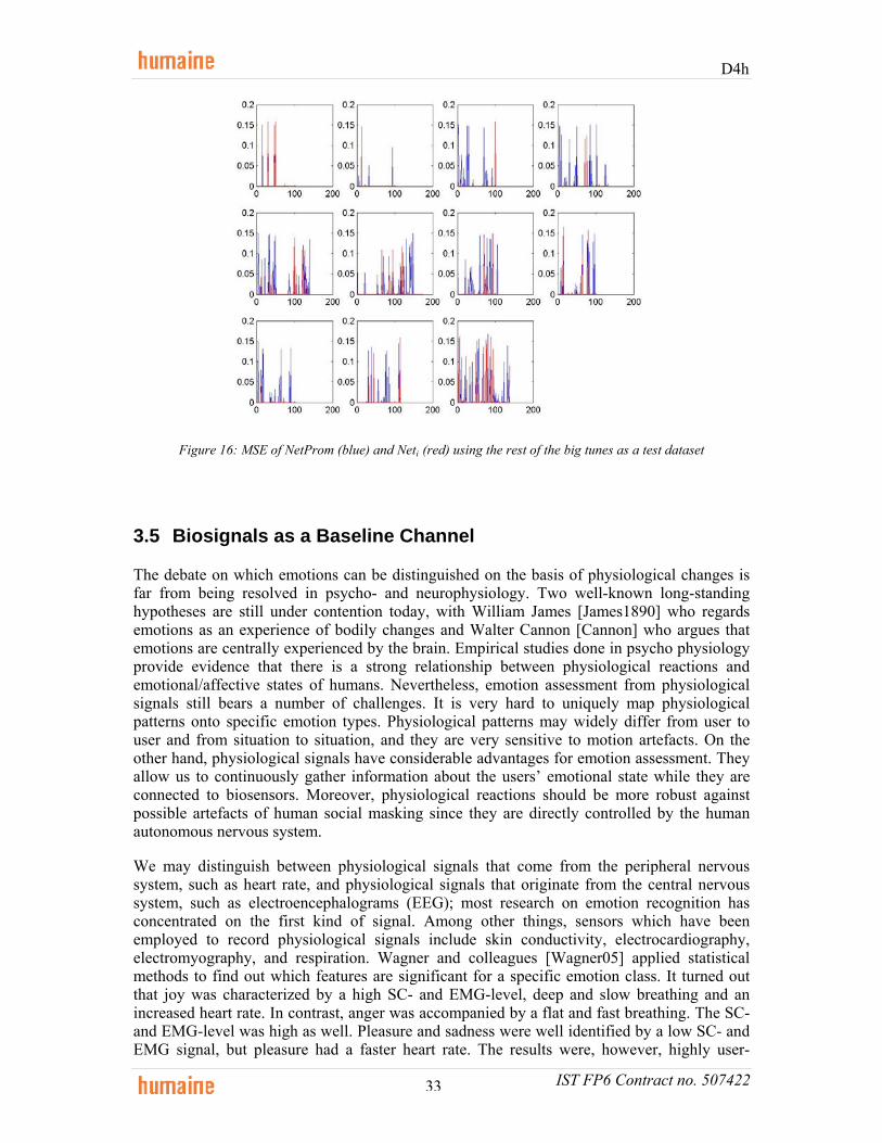
D4h


Figure 16: MSE of NetProm (blue) and Neti (red) using the rest of the big tunes as a test dataset

3.5 Biosignals as a Baseline Channel

The debate on which emotions can be distinguished on the basis of physiological changes is far from being resolved in psycho- and neurophysiology. Two well-known long-standing hypotheses are still under contention today, with William James [James1890] who regards emotions as an experience of bodily changes and Walter Cannon [Cannon] who argues that emotions are centrally experienced by the brain. Empirical studies done in psycho physiology provide evidence that there is a strong relationship between physiological reactions and emotional/affective states of humans. Nevertheless, emotion assessment from physiological signals still bears a number of challenges. It is very hard to uniquely map physiological patterns onto specific emotion types. Physiological patterns may widely differ from user to user and from situation to situation, and they are very sensitive to motion artefacts. On the other hand, physiological signals have considerable advantages for emotion assessment. They allow us to continuously gather information about the users’ emotional state while they are connected to biosensors. Moreover, physiological reactions should be more robust against possible artefacts of human social masking since they are directly controlled by the human autonomous nervous system.

We may distinguish between physiological signals that come from the peripheral nervous system, such as heart rate, and physiological signals that originate from the central nervous system, such as electroencephalograms (EEG); most research on emotion recognition has concentrated on the first kind of signal. Among other things, sensors which have been employed to record physiological signals include skin conductivity, electrocardiography, electromyography, and respiration. Wagner and colleagues [Wagner05] applied statistical methods to find out which features are significant for a specific emotion class. It turned out that joy was characterized by a high SC- and EMG-level, deep and slow breathing and an increased heart rate. In contrast, anger was accompanied by a flat and fast breathing. The SC- and EMG-level was high as well. Pleasure and sadness were well identified by a low SC- and EMG signal, but pleasure had a faster heart rate. The results were, however, highly user-

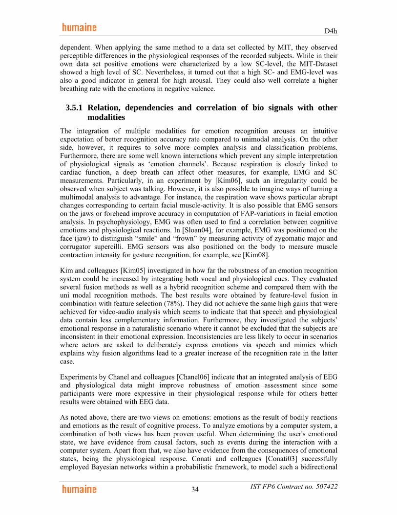
D4h


dependent. When applying the same method to a data set collected by MIT, they observed perceptible differences in the physiological responses of the recorded subjects. While in their own data set positive emotions were characterized by a low SC-level, the MIT-Dataset showed a high level of SC. Nevertheless, it turned out that a high SC- and EMG-level was also a good indicator in general for high arousal. They could also well correlate a higher breathing rate with the emotions in negative valence.

3.5.1 Relation, dependencies and correlation of bio signals with other modalities

The integration of multiple modalities for emotion recognition arouses an intuitive expectation of better recognition accuracy rate compared to unimodal analysis. On the other side, however, it requires to solve more complex analysis and classification problems. Furthermore, there are some well known interactions which prevent any simple interpretation of physiological signals as ‘emotion channels’. Because respiration is closely linked to cardiac function, a deep breath can affect other measures, for example, EMG and SC measurements. Particularly, in an experiment by [Kim06], such an irregularity could be observed when subject was talking. However, it is also possible to imagine ways of turning a multimodal analysis to advantage. For instance, the respiration wave shows particular abrupt changes corresponding to certain facial muscle-activity. It is also possible that EMG sensors on the jaws or forehead improve accuracy in computation of FAP-variations in facial emotion analysis. In psychophysiology, EMG was often used to find a correlation between cognitive emotions and physiological reactions. In [Sloan04], for example, EMG was positioned on the face (jaw) to distinguish “smile” and “frown” by measuring activity of zygomatic major and corrugator supercilli. EMG sensors was also positioned on the body to measure muscle contraction intensity for gesture recognition, for example, see [Kim08].

Kim and colleagues [Kim05] investigated in how far the robustness of an emotion recognition system could be increased by integrating both vocal and physiological cues. They evaluated several fusion methods as well as a hybrid recognition scheme and compared them with the uni modal recognition methods. The best results were obtained by feature-level fusion in combination with feature selection (78%). They did not achieve the same high gains that were achieved for video-audio analysis which seems to indicate that that speech and physiological data contain less complementary information. Furthermore, they investigated the subjects’ emotional response in a naturalistic scenario where it cannot be excluded that the subjects are inconsistent in their emotional expression. Inconsistencies are less likely to occur in scenarios where actors are asked to deliberately express emotions via speech and mimics which explains why fusion algorithms lead to a greater increase of the recognition rate in the latter case.

Experiments by Chanel and colleagues [Chanel06] indicate that an integrated analysis of EEG and physiological data might improve robustness of emotion assessment since some participants were more expressive in their physiological response while for others better results were obtained with EEG data.

As noted above, there are two views on emotions: emotions as the result of bodily reactions and emotions as the result of cognitive process. To analyze emotions by a computer system, a combination of both views has been proven useful. When determining the user's emotional state, we have evidence from causal factors, such as events during the interaction with a computer system. Apart from that, we also have evidence from the consequences of emotional states, being the physiological response. Conati and colleagues [Conati03] successfully employed Bayesian networks within a probabilistic framework, to model such a bidirectional

D4h


derivation of emotional states from its causes as well as its consequences in a game-like tutor system.

3.5.2 Augsburg Biosignal Toolbox (AuBT) Augsburg Biosignal Toolbox (AuBT) provides tools to analyse physiological signals in the face of emotion recognition. It consists of a bunch of Matlab functions which have been developed to meet the following tasks:

• extract features from physiological signals

• automatically select the relevant features

• use these features to train and evaluate a classifier

A graphical user interface (AuBTgui) serves as interface between user and toolbox. It provides an easy and fast way to analyze new data and gives access to all functions without a long period of vocational adjustment. AuBT comes along with two corpora: a corpus containing physiological data of a single user in four different emotional states and a corpus containing physiological data recorded from a single user under varying stress. For more information and to obtain the toolbox, visit its website [6] or the Humaine portal.

D4h


4 Links to other work packages

4.1 Annotation of large databases – expressivity features

As mentioned before, some of the video clips which were processed during the project were problematic either due to the unconstrained expressivity and motion of the subjects or the extreme compression which eliminated a substantial part of colour information and resolution. The fall-back solution, especially in the case of the emoTV clips [22], but also with other datasets [18], was to locate and track the hand and head segments, and provide statistical measures of their motion.

The general process involves the creation of moving skin masks, namely skin color areas that are tracked between subsequent frames (see Figure 17). By tracking the centroid of those skin masks, we produce an estimate of the user’s movements. A priori knowledge concerning the human body and the circumstances when filming the gestures was incorporated into the module indicating the different body parts (head, right hand, left hand). For each frame a skin color probability matrix is computed by calculating the joint probability of the Cr/Cb image values. The skin color mask is then obtained from the skin probability matrix using thresholding. Possible moving areas are found by thresholding the pixels’ difference between the current frame and the next, resulting in the possible-motion mask. This mask does not contain information about the direction or the magnitude of the movement, but is only indicative of the motion and is used to accelerate the algorithm by concentrating tracking only in moving image areas. Both color and motion masks contain a large number of small objects due to the presence of noise and objects with color similar to the skin. To overcome this, morphological filtering is employed on both masks to remove small objects. All described morphological operations are carried out with a disk-structuring element with a radius of 1% of the image width. The distance transform of the color mask is first calculated and only objects above the desired size are retained. These objects are used as markers for the morphological reconstruction of the initial color mask. The color mask is then closed to provide better centroid calculation. For the next frame, a new moving skin mask is created, and a one-to-one object correspondence is performed. Object correspondence between two frames is performed on the color mask and is based on object centroid distance for objects of similar (at least 50%) area. In the case of hand object merging and splitting, e.g., in the case of clapping, we establish a new matching of the left-most candidate object to the user’s right hand and the right-most object to the left hand. The Sagittal plane information of the gesture was ignored since it would require depth information from the video stream and it would make the performance of the proposed algorithm very poor or would require a side camera and parallel processing of the two streams. The described algorithm is lightweight, allowing a rate of around 12 fps on a usual PC during our experiments, which is enough for continuous gesture tracking. The object correspondence heuristic makes it possible to individually track the hand segments correctly, at least during usual meaningful gesture sequences. In addition, the fusion of color and motion information eliminates any background noise or artifacts, thus reinforcing the robustness of the proposed approach.

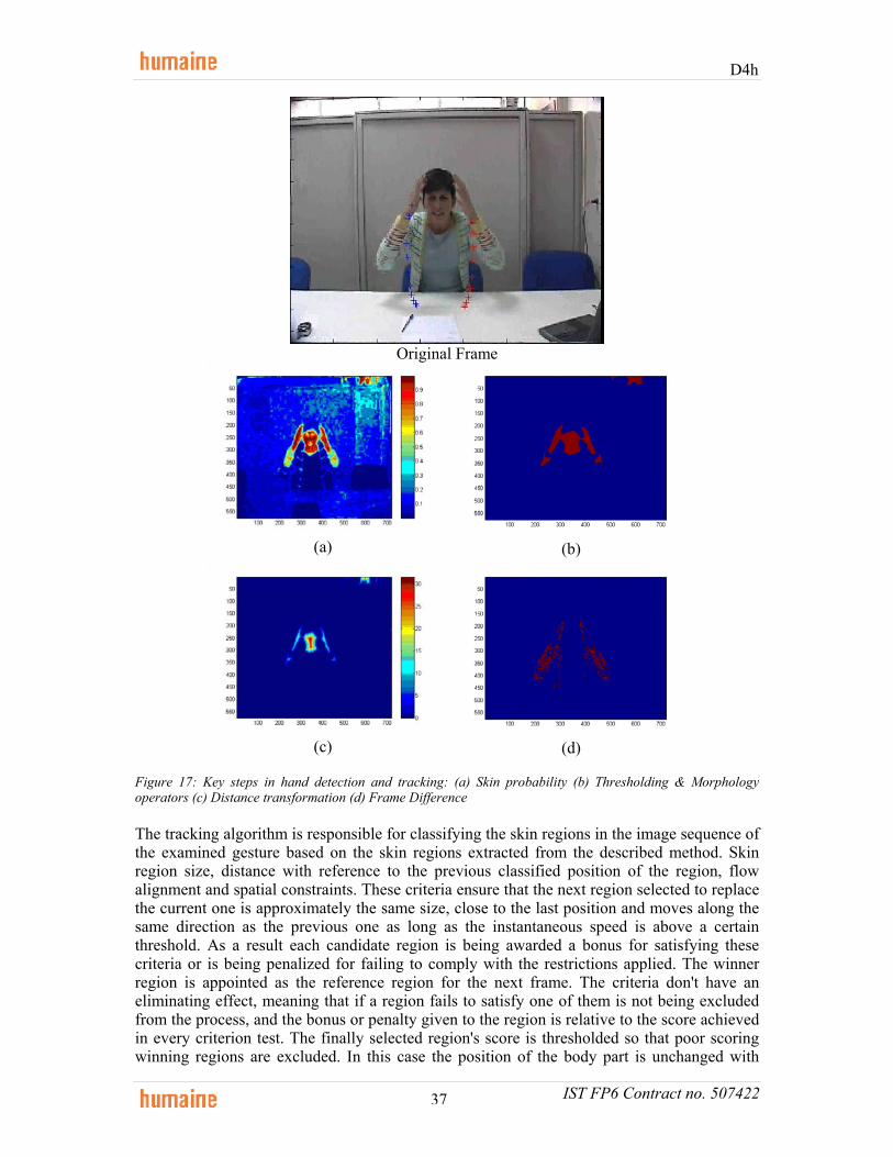
D4h


Original Frame

(a)

(b)

(c)

(d)

Figure 17: Key steps in hand detection and tracking: (a) Skin probability (b) Thresholding & Morphology operators (c) Distance transformation (d) Frame Difference

The tracking algorithm is responsible for classifying the skin regions in the image sequence of the examined gesture based on the skin regions extracted from the described method. Skin region size, distance with reference to the previous classified position of the region, flow alignment and spatial constraints. These criteria ensure that the next region selected to replace the current one is approximately the same size, close to the last position and moves along the same direction as the previous one as long as the instantaneous speed is above a certain threshold. As a result each candidate region is being awarded a bonus for satisfying these criteria or is being penalized for failing to comply with the restrictions applied. The winner region is appointed as the reference region for the next frame. The criteria don't have an eliminating effect, meaning that if a region fails to satisfy one of them is not being excluded from the process, and the bonus or penalty given to the region is relative to the score achieved in every criterion test. The finally selected region's score is thresholded so that poor scoring winning regions are excluded. In this case the position of the body part is unchanged with

D4h


reference to that in the previous frame. This feature is especially useful in occlusion cases when the position of the body part remains the same as just before occlusion occurs. After a certain number of frames the whole process is reinitialized so that a possible misclassification is not propagated. Head and head occlusion is tackled with the following simplistic yet efficient method. Suppose occlusion occurs at frame n and ceases to exist at frame k. The position of the hand during the occlusion phase (frames n-k) is considered to be the position of the hand at frame n-1. After frame k the detection and tracking algorithm for the specific hand continues normally. Figure 18 demonstrates the hand and head trajectories produced by the proposed algorithm when applied to the GEMEP database [42].

Figure 18: Hand and head tracking results

4.1.1 Calculation of gesture expressivity features Expressivity of behaviour is an integral part of the communication process as it can provide information on the current emotional state, mood, and personality of a person [20]. Many researchers have investigated human motion characteristics and encoded them into dual categories such as slow/fast, small/expansive, weak/energetic, small/large, unpleasant/pleasant. To model expressivity, in our work, we use the six dimensions of behavior described in [7], as a more accomplished way to describe the expressivity, since it tackles all the parameters of expression of emotion. Five parameters which model expressivity have been defined at the analysis level, as a subset of the above-mentioned six dimensions of behaviour, namely overall activation, spatial extent, temporal, fluidity and power

Overall activation is considered as the quantity of movement during a conversational turn. In our case it is computed as the sum of the motion vectors’ norm

0| ( ) | | ( ) |

n

iOA r i l i

=

= +∑rr

Spatial extent is modeled by expanding or condensing the entire space in front of the agent that is used for gesturing and is calculated as the maximum Euclidean distance of the position of the two hands: max(| ( ( ) ( )) |)SE d r i l i= −

rr . The average spatial extent is also calculated for normalization reasons. The temporal expressivity parameter of the gesture signifies the duration of the movement while the speed expressivity parameter refers to the arm movement

D4h


during the gesture’s stroke phase (e.g., quick versus sustained actions). Gestures have three phases: preparation, stroke and retraction. The real message is in the stroke, whilst the preparation and retraction elements consist of moving the arms to and from the rest position, to and from the start and end of the stroke. Fluidity differentiates smooth/graceful from sudden/jerky ones. This concept seeks to capture the continuity between movements, as such, it seems appropriate to modify the continuity of the arms’ trajectory paths as well as the acceleration and deceleration of the limbs. To extract this feature from the input image sequences we calculate the sum of the variance of the norms of the motion vectors. Power actually is identical with the first derivative of the motion vectors calculated in the first steps.

4.2 Synthesis of expressive gestures

Communicative capabilities of conversational agents could be significantly improved if they could also convey the expressive component of physical behavior. Starting from the results reported in [20], we have defined and implemented [7] a set of five parameters that affect the quality of the agent's behavior, that is the movement's spatial volume (SPC), speed (TMP), energy (PWR), fluidity (FLT) and repetitivity (REP). Thus, the same gestures or facial expressions are performed by the agent in a qualitatively different way depending on this set of parameters.

Table 11 shows the effect that each one of expressivity parameter has on the production of head movements, facial expressions and gestures. The SPC parameter modulates the amplitude of the movement of arms, wrists (involved in the animation of a gesture), head and eyebrows (involved in the animation of a facial expression); it influences how wide or narrow their displacement will be during the final animation. For example let us consider the eyebrows raising in the expression of surprise: if the value of the Spatial Extent parameter is very high the final position of the eyebrows will be very high in the forehead (i.e. the eyebrows move under a strong of muscular contraction). The TMP parameter shortens or lengthens the motion of the preparation and retraction phases of the gesture as well as the onset and offset duration for facial expression. On of the effect on the face is to speed up or slow down the rising/lowering of the eyebrows. The agent animation is generated by defining some key frames and computing the interpolation curves passing through these frames. The FLT and PWR parameters act on the interpolation curves. Fluidity increases/reduces the continuity of the curves allowing the system to generate more/less smooth animations. Let us consider its effect on the head: if the value of the Fluidity parameter is very low the resulting curve of the head movement will appear as generated through linear interpolation. Thus, during its final animation the head will have a jerky movement. Power introduces a gesture/expression overshooting, that is a little lapse of time in which the body part involved by the gesture reaches a point in space further than the final one. For example the frown displayed in the expression of anger will be stronger for a short period of time, and then the eyebrows will reach the final position. The last parameter, REP, exerts an influence on gestures and head movements. It increases the number of stroke of gestures to obtain repetition of the gestures themselves in the final animation. Let us consider the gesture "wrists going up and down in front of the body with open hands and palms up", a high value of the Repetition parameter will increase the number of the up and down movements. On the other hand this parameter decreases the time period of head nods and head shakes to obtain more nods and shakes in the same lapse of time.

Table 11 can be better understood with two intuitive examples. SPC affects the amplitude of the agent’s head facial and body gestures: if a high value of SPC is selected and the agent has to perform a smile, the corners of her lips will widen and turn up the maximum. TMP affects the speed of head movements, facial expressions appearance and disappearance and gestures

D4h


preparation and retraction. Then, for example, if a low value of TMP is selected and the agent has to nod, show a frown and perform a beat gesture, her head nod will be sluggish, her eyebrows will knit slowly, and she will move her arm slowly before the stroke of the beat gesture.

Head Facial expression Gesture

SPC wider/narrower movement

increased/decreased emotion arousal

wider/narrower movement

TMP shorter/longer movement speed

shorter/longer onset and offset

shorter/longer speed of preparation and retraction phases

FLT increases/reduces

continuity of head movement

increases/reduces continuity of movement

increases/reduces continuity between

consecutive gestures

PWR higher/shorter

head overshooting

higher/shorter movement acceleration

more/less stroke

acceleration

REP more/less number of

nods and shakes

not implemented

yet

more/less number of repetitions

of the same stroke

Table 11: Effects of Expressivity parameters over head, facial expression and gesture

The synthesis module is able to reproduce a large set of facial expressions, the universals proposed by Ekman [33] and many others obtained as a combination of them. Gestures are computed through the interpolation of a sequence of static positions obtained defining shoulder and arm rotation (arm position), hand shape (chosen in a set of predefined shapes) and palm orientation. So the synthesis module can successfully reproduce beat and iconic gestures whereas circular gestures cannot be performed.

From the point of view of implementation, our agent system produces animation data in MPEG4-compliant FAP/BAP format, which in turn drive a facial and skeletal body model in OpenGL. A set of parameters, called Facial Animation Parameters (FAPs) and Body Animation Parameters (BAPs), are used to animate the face and the body. By specifying values for FAPs and BAPs, we can specify facial expressions and body positions. The animation is specified by a sequence of keyframes. A keyframe is defined by a set of FAP or BAP values to be reached. Animation is obtained by interpolating between these keyframes. Interpolation is performed using TCB (Tension, Continuity, Bias) splines [11].

The expressivity parameters are implemented by changing the TCB parameters of the interpolating splines and by scaling the values and changing the timing of the keyframes points. For example, the SPC parameter will influence the value of the keyframes by scaling them. The higher the SPC is, the wider the interpolating curves will be and so facial expressions will be more visible on the face and gestures wider. The FLD parameter will modulate the Continuity parameters of the splines, making them becoming smoother (high FLD) or jerkier (low FLD).

4.2.1 Implementation Section 4.1 described the general framework of a system able to analyze a real scene and cater for animating a virtual agent. Here we present a scenario that is a partial implementation of this framework. Currently our system (Figure 19) is able to extract data from the video

D4h


stream, process it and generate the animation of virtual agent. The final animation we aim to obtain consists on reproducing the gesture which is manually communicated to the agent and the facial expression that the system deduces from those performed by an actor.

Figure 19: Application scenario

Figure 20: Subjects of the scenario

Gesture class quadrant of Whissel’s wheel explain (0,0), (+, +), (-, +), (-, -) oh my god (+, +), (-, +) leave me alone (-, +), (-, -) raise hand (0,0), (+, +), (-, -) bored (-, -) wave (0,0), (+, +), (-, +), (-, -) clap (0,0), (+, +), (-, +), (-, -)

Table 12: Acted Emotions

The input is coming from an acted action performed by an actor. The action consists of a gesture accompanied by a facial expression. Both the type of the gesture and the type of the expression are explicitly requested from the actor and previously described to him in natural language in an acted portrayal scenario [42] (for example, the actor is asked "to wave his right hand in front of the camera while showing a happy face"). Real life corpus was considered but was not selected because expressions sampled in real-life occur in specific contexts which often cannot be reproduced, their verbal content and the overall quality of the recordings cannot be controlled, one person is usually recorded in only one or very few different

D4h


emotional states, and it is not always clear on which grounds and how these states should be labeled.

The Perception module analyzes the resulting video extracting the expressivity parameters of the gesture and the displacement of facial parts that is used to derive the FAPs values corresponding to the expression performed. The FAPs values and the Expressivity parameters are sent to the Expression Recognition module. If the facial expression corresponds to one of the prototypical facial expression of emotions, this module is able to derive its symbolic name (emotion label) from the FAPs values received in input; if not the FAPs values are used. Instead, the symbolic name of the gesture is sent manually because the actual system is not able to extract the gesture shape from the data yet. In the near future, we would like also to implement a Planning module (represented in Figure 19 with a dashed box) that could compute a modulation either of the expressivity parameters or the emotion. Finally the animation, consisting of variation of FAPs and BAPs values during time, is computed in the Generation module which contains the Face and the Gesture Engine. The Face Engine (which actually computes also the head movements of the agent) receives in input either the emotion label (or a list of FAPs) and a set of expressivity parameters. The way in which the facial expressions appear and head movements are performed is modulated by the expressivity parameters as explained in Section 4, Table 1. In the same way, the Gesture Engine receives in input a gesture label and a set of expressivity parameters. So the gestures produced by the Gesture Engine are influenced by the actual set of expressivity parameters, as explained in Table 11.

The input image sequences of the presented system are videos captured at an acted session including 7 actors (Figure 20), every one of them performing 7 gestures (Table 12). Each gesture was performed several times with the student-actor impersonating a different situation. The gestures performed are: “explain”, “oh my god” (both hands over head), “leave me alone”, “raise hand” (draw attention), “bored” (one hand under chin), “wave”, “clap”. Table 12 indicates which emotion repetitions were performed for every specific gesture. For example gesture “wave” was performed 4 times one for the neutral emotion and three ( (+, +), (-, +), (-, -) ) for specific quadrants of the Whissel’s wheel. Some combinations were not included in the scenario since it did not make much sense in performing the “bored” gesture in a happy (+,+) mood.

D4h


Figure 21: Head and hand tracking results on scenario subjects

Figure 22 shows the values of the expressivity features using the previously described algorithm on the gestures performed during the described experiment. Figure 23 proves the soundness of the overall module for calculating expressivity features by indicating the expected result. This would be that gestures belonging to the positive activation half-plane have higher scores on Overall Activation and Power in comparison to those belonging to the negative activation half-plane.

(a) overall activation (b) spatial extent (c) fluidity (d) power/energy

Figure 22: Mean Expressivity features values for every gesture class

(a) (b)

Figure 23: Mean values of Overall Activation (a) and Power (b) for positive and negative values of activation respectively

D4h


(a) (b) (c)

Figure 24: Demonstration of behaviour mimicry

Figure 24 demonstrates three instances of behavior mimicry. The gesture being mimicked is “raise hand”. (a) instance is neutral where as (b) is happy (+/+ quadrant) and (c) is sad (-/- quadrant). Not all expressivity features can be observed from just an instance of the animation but Spatial Extent is very easily distinguishable for both the gestural and the facial aspect of the animation.

D4h


5 References [1] A. Batliner, S. Steidl, B. Schuller, D. Seppi, K. Laskowski, T. Vogt, L. Devillers, L. Vidrascu, N. Amir, L. Kessous, V. Aharonson, Combining Efforts for Improving Automatic Classification of Emotional User States, In Proceedings of IS-LTC 2006, 2006. [2] A. Batliner, S. Steidl, B. Schuller, D. Seppi, T. Vogt, L. Devillers, L. Vidrascu, N. Amir, L. Kessous, V. Aharonson, The Impact of F0 Extraction Errors on the Classification of Prominence and Emotion, in Proceedings of ICPhS 2007. [3] A. Batliner, S. Steidl, C. Hacker, E. Noeth, Private emotions versus social interaction: a data-driven approach towards analysing emotion in speech, User Modeling and User-Adapted Interaction, Springer, Volume 18, Numbers 1-2 / February, 2008. [4] A. Batliner, S. Steidl, E. Noeth, Laryngealizations and Emotions: How Many Babushkas?, in Proceedings of ParaLing 2007 (to appear) [5] A. Yilmaz and M. A. Shah, Automatic feature detection and pose recovery for faces, Asian Confer-ence on Computer Vision, 23-25, 2002. [6] Augsburg Biosignal Toolbox (AuBT), http://mm-werkstatt.informatik.uni-augsburg.de/project_details.php?id=33, Last retrieved Dec 30, 2007. [7] B. Hartmann, M. Mancini, C. Pelachaud, Formational parameters and adaptive prototype instantiation for MPEG-4 compliant gesture synthesis. In Computer Animation'02, Geneva, Switzerland. IEEE Computer Society Press, 2002. [8] B. Schuller, A. Batliner, D. Seppi, S. Steidl, T. Vogt, J. Wagner, L. Devillers, L. Vidrascu, N. Amir, L. Kessous, V. Aharonson, The Relevance of Feature Type for the Automatic Classification of Emotional User States: Low Level Descriptors and Functionals, in Proceedings of Interspeech 2007, Antwerpen, 2007 (to appear) [9] B. Schuller, D. Seppi, A. Batliner, A. Maier, S. Steidl, Towards more Reality in the Recognition of Emotional Speech, in Proceedings of ICASSP, Honolulu, 2007, pp. 941-944. [10] D. Beymer, M. Flickner, M., Eye gaze tracking using an active stereo head, Conference on Computer Vision and Pattern Recognition (CVPR), Vol. 2, pp. 451–458, 2003. [11] D. Kochanek, R. Bartels, Interpolating splines with local tension, continuity, and bias control. In Christiansen, H., ed.: Computer Graphics (SIGGRAPH'84 Proceedings). Volume 18, pp. 33-41, 1984. [12] D. Park, M. A. EL-Sharkawi, and R. J. Marks II, An adaptively trained neural network, IEEE Trans. Neural Networks, vol. 2, pp. 334–345, 1991. [13] Elman, J. L. (1990). Finding structure in time. Cognitive Science, 14, 179-211. [14] Elman, J. L. (1991). Distributed representations, simple recurrent networks, and grammatical structure. Machine Learning, 7, 195-224. [15] F. Hoenig, A. Batliner, E. Noeth, Real-time Recognition of the Affective User State with Physiological Signals, R. Cowie and F. de Rosis (Eds.), Affective Computing and Intelligent Interaction, Doctoral Consortium, Lisbon, Portugal 2006, pp. 1-8. [16] F. Hoenig, http://www5.informatik.uni-erlangen.de/Personen/hoenig/biosignale/, last retrieved Dec. 30, 2007. [17] FP5 IST ERMIS Emotionally Rich Man-Machine Interaction Systems, http://www.image.ntua.gr/ermis/, last retrieved Dec. 30, 2007.

D4h


[18] G. Caridakis, A. Raouzaiou, E. Bevacqua, M. Mancini, K. Karpouzis, L. Malatesta and C. Pelachaud, Virtual agent multimodal mimicry of humans, Language Resources and Evaluation, Special issue on Multimodal Corpora, Springer. [19] G. W. Williams, Comparing the joint agreement of several raters with another rater, Biometrics, vol 32, pp. 619-627, 1976. [20] H.G. Wallbott, K. Scherer, Cues and channels in emotion recognition. Journal of Personality and Social Psychology, 51(4):690-699, 1986. [21] I. Cohen, N. Sebe, A. Garg, L.S. Chen, T.S. Huang, Facial expression recognition from video sequences: temporal and static modeling, Computer Vision and Image Understanding 91 (2003) 160–187. [22] J. -C. Martin, G. Caridakis, L. Devillers, K. Karpouzis, S. Abrilian, Manual annotation and automatic image processing of multimodal emotional behaviors: validating the annotation of TV interviews, Personal and Ubiquitous Computing, Special issue on Emerging Multimodal Interfaces, Springer, 2007. [23] J. Taylor, N. Fragopanagos, Modelling human attention and emotions, Proceedings of the 2004 IEEE International Joint Conference on Neural Networks, Volume: 1, pp. 501 – 506. [24] J. Taylor, N. Fragopanagos, The interaction of attention and emotion, Neural Networks , Volume 18, Issue 4, May 2005, pp. 353 – 369. [25] J. W. Young, Head and Face Anthropometry of Adult U.S. Civilians, FAA Civil Aeromedical Institute, 1963-1993 (final report 1993) [26] J. Wagner, J. Kim, E. André, From Physiological Signals to Emotions: Implementing and Comparing Selected Methods for Feature Extraction and Classification, In IEEE International Conference on Multimedia & Expo (ICME 2005), 2005. [27] J.G. Wang, E. S. and Venkateswarku, R., Eye gaze estimation from a single image of one eye, 9th IEEE International Conference on Computer Vision, 2003. [28] J.Y. Bouguet, Pyramidal Implementation of the Lucas Kanade Tracker, OpenCV Documentation, http://opencvlibrary.sourceforge.net/, Last retrieved Dec 30, 2007. [29] M. Pantic and I. Patras, 'Dynamics of Facial Expression: Recognition of Facial Actions and Their Temporal Segments from Face Profile Image Sequences', IEEE Transactions on Systems, Man and Cybernetics - Part B, vol. 36, no. 2, pp. 433-449, April 2006. [30] M. Wallace, S. Ioannou, A. Raouzaiou, K. Karpouzis, S. Kollias, Dealing with Feature Uncertainty in Facial Expression Recognition Using Possibilistic Fuzzy Rule Evaluation, International Journal of Intelligent Systems Technologies and Applications, Volume 1, Number 3-4, 2006. [31] N. Doulamis, A. Doulamis and S. Kollias, On-Line Retrainable Neural Networks: Improving Performance of Neural Networks in Image Analysis Problems, IEEE Transactions on Neural Networks, vol. 11, no.1, pp.1-20, January 2000. [32] O. Jesorsky, K. J. Kirchberg and R. W. Frischholz, Robust face detection using the Hausdorff distance, 3rd Conf. AVBPA, 90-95, 2001. [33] P. Ekman, Basic emotions. In Dalgleish, T. and Power, M. J., eds., Handbook of Cognition & Emotion, pages 301{320. John Wiley, New York, 1999. [34] P. Viola and M. Jones, Rapid object detection using a boosted cascade of simple features, IEEE Com-puter Vision and Pattern Recognition, Vol. 1, pp. 511-518, 2001.

D4h


[35] R. Cowie, E. Douglas-Cowie, S. Savvidou, E. McMahon, M. Sawey, and M. Schroeder, ’Feeltrace’: An instrument for recording perceived emotion in real time, in Proc. ISCA Workshop on Speech and Emotion, 2000, pp. 19–24. [36] S. Asteriadis, P. Tzouveli, K. Karpouzis, S. Kollias, Non-verbal feedback on user interest based on gaze direction and head pose, Proc. 2nd International Workshop on Semantic Media Adaptation and Personalization (SMAP'07), London, UK, December 17-18, 2007. [37] S. Haykin, Neural Networks: A Comprehensive Foundation, Prentice Hall International, 1999. [38] S. Ioannou, A. Raouzaiou, V. Tzouvaras, T. Mailis, K. Karpouzis, S. Kollias, Emotion recognition through facial expression analysis based on a neurofuzzy network, Special Issue on Emotion: Understanding & Recognition, Neural Networks, Elsevier, Volume 18, Issue 4, May 2005, pp. 423-435. [39] S. Ioannou, G. Caridakis, K. Karpouzis, S. Kol-lias, Robust Feature Detection for Facial Expression Recognition, EURASIP Journal on Image and Video Processing, Hindawi Publishing Corporation, 2007. [40] SensoMotoric Instruments. EyeLink Gaze Tracking. www.smi.de [41] T. Baenziger, H. Pirker, K. Scherer, GEMEP - geneva multimodal emotion portrayals: a corpus for the study of multimodal emotional expressions, In L. Devillers et al. (Ed.), Proceedings of LREC'06 Workshop on Corpora for Research on Emotion and Affect, pp. 15-19, Genoa. Italy, 2006. [42] T. Baenziger, H. Pirker, K. Scherer, GEMEP - Geneva multimodal emotion portrayals: a corpus for the study of multimodal emotional expressions. In L. Devillers et al. (Ed.), Proceedings of LREC'06 Workshop on Corpora for Research on Emotion and Affect (pp. 15-19), Genoa, Italy, 2006. [43] Zeng, Z., Tu, J., Liu, M., Huang, T.S., Pianfetti, B., Roth D. and Levinson, S. (2007), Audio-visual Affect Recognition, IEEE Transactions on Multimedia, Vol. 9, No. 2, February 2007, 424-428.

D4h


6 WP4 Deliverables (all of these are available on the portal)

D

el. n

o

Del

iver

able

na

me

D4a Workshop proceedings: Signs�

D4b Preliminary Plans for Exemplars: Signals & Signs�

D4c potential exemplars signals to signs�

D4d Proposal for exemplar and work towards it: Signs and Signals�

D4e Report on utility of features in auditory, visual and physiological modalities (Confidential)�

D4f Mid-term report on signal to emotion exemplar progress�

D4g Pre-completion report on exemplar�

Documents

D4h-Final report on WP4 - emotion-research.netemotion-research.net/projects/humaine/deliverables/D4h-Final report... · D4h 2 IST FP6 Contract no. 507422 IST project contract no