D4.3 THIRD REPORT ON PILOT REQUIREMENTScoegss.eu/wp-content/uploads/2018/02/D4.3.pdf · D4.3 Third Report on Pilot Requirements 5 List of Figures Figure 3.1 – The implementation

D4.3 – THIRD REPORT ON PILOT REQUIREMENTS

Grant Agreement 676547

Project Acronym CoeGSS

Project Title Centre of Excellence for Global Systems Science

Topic EINFRA-5-2015

Project website http://www.coegss-project.eu

Start Date of project October 1, 2015

Duration 36 months

Deliverable due date 30.11.2017

Actual date of submission 30.11.2017

Dissemination level Public

Nature Report

Version 2 (after internal review)

Work Package 4

Lead beneficiary GCF

Responsible scientist/administrator Sarah Wolf

Contributor(s) Margaret Edwards, Steffen Fürst, Andreas Geiges,

Jette von Postel, Enrico Ubaldi

Internal reviewers Jochen Buchholz, Cezar Ionescu

Keywords Requirements, Synthetic Information System, Easy Access, Simulation Analysis

Total number of pages: 27

D4.3 Third Report on Pilot Requirements

1

Copyright (c) 2016 Members of the CoeGSS Project.

The CoeGSS (“Centre of Excellence for Global Systems Science”) project is

funded by the European Union. For more information on the project please

see the website http:// http://coegss-project.eu/

The information contained in this document represents the views of the CoeGSS as of the date

they are published. The CoeGSS does not guarantee that any information contained herein is

error-free, or up to date.

THE CoeGSS MAKES NO WARRANTIES, EXPRESS, IMPLIED, OR STATUTORY, BY PUBLISHING

THIS DOCUMENT.

Version History

Name Partner Date

From Sarah Wolf GCF

First Version for internal review Nov, 2017

Second Version for submission Nov, 2017

Reviewed by Jochen Buchholz

Cezar Ionescu

HLRS

Chalmers

Nov, 2017

Nov, 2017

Approved by ECM ATOS,HLRS,UP Nov, 2017


2

Abstract

This deliverable is the third report on pilot requirements to the Centre of Excellence for Global

Systems Science, and hence acts as the third and last official version of the living document

begun with D4.1 and continued with D4.2. It complements the previous versions with

requirements that became apparent as the project work progressed; in particular, pilot

models have been implemented now need to be thoroughly analysed.

The three pilot studies represent typical applications of Global Systems Science. They develop

synthetic information systems, that is, computer simulation based tools to help explore and

understand global challenges. In particular, the Health Habits pilot addresses the tobacco

epidemics, the Green Growth pilot studies the diffusion of electric vehicles in the global car

market, and the Global Urbanisation pilot analyses two-way relations between transport

infrastructure and real-estate pricing.

Previous requirements remain valid without being repeated in this version of the deliverable,

and further discussion of the requirements presented here is foreseen in working groups as

needed.


3

Table of Contents

List of Abbreviations ................................................................................................................... 4

List of Figures .............................................................................................................................. 5

1 Introduction ......................................................................................................................... 6

2 Easy Access .......................................................................................................................... 7

3 Simulation output analysis .................................................................................................. 8

4 Next steps .......................................................................................................................... 23

5 References ......................................................................................................................... 24


4

List of Abbreviations ABM Agent-Based Model

CoeGSS Centre of Excellence for Global System Science

GB Gigabyte

GSS Global Systems Science

HLRS High-Performance Computing Centre Stuttgart (a site in CoeGSS)

HPC High Performance Computing

HPDA High Performance Data Analysis

IDE Integrated Development Environment

MCMC Markov-Chain-Monte-Carlo

MoTMo Mobility Transition Model

MPI Message Passing Interface

PSNC Poznan Supercomputing and Networking Center (a site in CoeGSS)

SIS Synthetic Information System

SSH Secure Shell

TB Terabyte

WP Work Package


5

List of Figures Figure 3.1 – The implementation of a MCMC chain and an overview of the parallel tempering

scheme with four chains featuring four different temperatures ...................................... 9

Figure 3.2 – Single chain and the colder chain in an eight-chains parallel tempering evolution

for an MCMC process ....................................................................................................... 11

Figure 3.3 – Left side: Model run and post-analysis is performed on separated hardware. Right

side: HCP hardware is used to perform model runs and post-analysis. .......................... 14

Figure 3.4 – Simple example: real surface to explore in the parameter space ....................... 16

Figure 3.5 – Simple example: simulated points in the parameter space ................................. 17

Figure 3.6 – Simple example: accuracy .................................................................................... 17

Figure 3.7 – Simple example: comparing the accuracy reached by the algorithmic approach vs

a systematic approach for a given number of simulations .............................................. 18

Figure 3.8 – Simple example: ratio of the number of simulations required by the algorithmic

vs the systematic approach, to achieve a given level of accuracy ................................... 19


6

1 Introduction Following up on D4.1 and D4.2, this deliverable presents an update on pilot requirements to

the Centre of Excellence for Global Systems Science (CoeGSS).

The pilot studies of CoeGSS address three example challenges in different fields of Global

Systems Science (GSS). The Health Habits pilot studies smoking epidemics, the Green Growth

pilot models the diffusion of electric vehicles in the global car fleet, and the Global

Urbanisation pilot relates transport infrastructure and real-estate pricing. Each pilot develops

a synthetic information system (SIS) for analysing potential evolutions of the global system

underlying the question that is addressed. Briefly summarised, this means a model is defined

and data collected in order to implement an agent-based model (ABM); agents are taken from

a synthetic population, which statistically matches the real-world population for relevant

aspects; simulations of the ABM are then analysed to explore and understand potential

evolutions of the system (for more detail, see D4.1 – First Report on Pilot Requirements and

D4.4 – First Status Report of the Pilots). Together, the pilot studies are thus working towards

defining the requirements for a framework for generating such synthetic information systems

that provide simulation tools to explore global systems.

Throughout the project work, requirements for the development of an HPC-based SIS for GSS

have been worked out. At the very beginning of the project, D4.1 specified the steps involved

in developing and using SIS, and provided initial requirements in terms of data and software

for the different pilots. Then, D4.2 further specified requirements on data collection and pre-

processing, synthetic populations, synthetic networks, a GSS-specific ABM-framework, and SIS

analysis tools. These points were treated with a level of detail adapted to the current state of

pilot in both cases. In particular, in a phase where model implementation was the main focus,

the requirements on an ABM-framework were a focus area in D4.2. In the meantime, pilot

models have been implemented and calibrated up to a point where now simulation analysis

plays a more important role. Therefore, this iteration of the pilot requirements focuses on

running model simulations and analysing these. First, Section 2 collects aspects of what pilot

(and more generally, GSS) modellers consider “easy access” to computing resources for

running models. Then, Section 3 describes different techniques the pilots want to use for

model simulation output analysis and specifies the requirements that come with them.

Section 4 concludes.


7

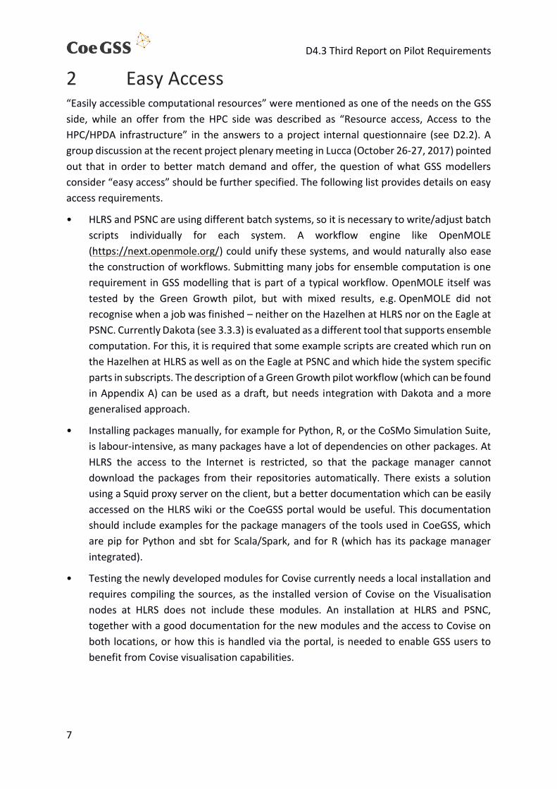
2 Easy Access “Easily accessible computational resources” were mentioned as one of the needs on the GSS

side, while an offer from the HPC side was described as “Resource access, Access to the

HPC/HPDA infrastructure” in the answers to a project internal questionnaire (see D2.2). A

group discussion at the recent project plenary meeting in Lucca (October 26-27, 2017) pointed

out that in order to better match demand and offer, the question of what GSS modellers

consider “easy access” should be further specified. The following list provides details on easy

access requirements.

• HLRS and PSNC are using different batch systems, so it is necessary to write/adjust batch

scripts individually for each system. A workflow engine like OpenMOLE

(https://next.openmole.org/) could unify these systems, and would naturally also ease

the construction of workflows. Submitting many jobs for ensemble computation is one

requirement in GSS modelling that is part of a typical workflow. OpenMOLE itself was

tested by the Green Growth pilot, but with mixed results, e.g. OpenMOLE did not

recognise when a job was finished – neither on the Hazelhen at HLRS nor on the Eagle at

PSNC. Currently Dakota (see 3.3.3) is evaluated as a different tool that supports ensemble

computation. For this, it is required that some example scripts are created which run on

the Hazelhen at HLRS as well as on the Eagle at PSNC and which hide the system specific

parts in subscripts. The description of a Green Growth pilot workflow (which can be found

in Appendix A) can be used as a draft, but needs integration with Dakota and a more

generalised approach.

• Installing packages manually, for example for Python, R, or the CoSMo Simulation Suite,

is labour-intensive, as many packages have a lot of dependencies on other packages. At

HLRS the access to the Internet is restricted, so that the package manager cannot

download the packages from their repositories automatically. There exists a solution

using a Squid proxy server on the client, but a better documentation which can be easily

accessed on the HLRS wiki or the CoeGSS portal would be useful. This documentation

should include examples for the package managers of the tools used in CoeGSS, which

are pip for Python and sbt for Scala/Spark, and for R (which has its package manager

integrated).

• Testing the newly developed modules for Covise currently needs a local installation and

requires compiling the sources, as the installed version of Covise on the Visualisation

nodes at HLRS does not include these modules. An installation at HLRS and PSNC,

together with a good documentation for the new modules and the access to Covise on

both locations, or how this is handled via the portal, is needed to enable GSS users to

benefit from Covise visualisation capabilities.

https://next.openmole.org/


8

3 Simulation output analysis In the iterative process of developing a GSS-SIS, as well as when using it, simulation output

analysis plays an important role. Dynamics in an ABM are defined on the micro-level: agents

are equipped with decision rules, and, agents, the networks between them, and their

environment can be equipped with update rules. The resulting overall system dynamics is not

described by given macro-level equations, but is observed in output from simulation runs.

Moreover, ABMs are generally stochastic, meaning that not single, but groups of simulation

runs need to be observed and thus analysed. One particular task that requires output analysis

is that of parameter calibration. This section presents three ways in which pilots intend to

carry out their model output analysis and specifies the corresponding requirements.

3.1 Markov-Chain-Monte-Carlo Markov-Chain-Monte-Carlo (MCMC) is a technique for performing integration with

simulations (Gilks, 2005; Gilks, Richardson, & Spiegelhalter, 1995). The goal of the MCMC

implementation is to expand the classical Monte Carlo integration technique to account for

cases in which the density distribution of the parameters is unknown. Specifically, suppose

that we want to evaluate the expectation value of a given function 𝑔(𝐩) over a probability

density 𝑓(𝐩):

⟨𝑔(𝐩)⟩𝑓 = ∫ 𝑔(𝐩)𝑓(𝐩)𝑑𝐩, (3.1)

where 𝐩 is an array of parameters and/or models unknown (e.g., missing data).

If we can draw sample 𝐩0, 𝐩1, ⋯ , 𝐩𝑁−1 independently from 𝑓(𝐩) we can approximate ⟨𝑔(𝐩)⟩𝑓

with the usual Monte Carlo integration:

⟨𝑔(𝐩)⟩𝑓 ≃1

𝑁∑ 𝑔(𝐩𝑖)

𝑁−1

𝑖=0

. (3.2)

In the Bayesian approach, 𝑓(𝐩) is rather a posterior distribution 𝑓(𝐩|𝐱) over the observed

data 𝐱. Moreover, 𝐩 may be high-dimensional and the functional form of 𝑓(𝐩|𝐱) may be non-

analytical so that generating an independent sampling from 𝑓(𝐩|𝐱) is generally unfeasible.

MCMC solves this issue by generating a Markov chain of dependent samples 𝐩0, 𝐩1, ⋯ , 𝐩𝑁−1,

where each parameter value 𝐩𝑖 depends on the previous value 𝐩𝑖−1 only and on the selected

update rule. The only requirement on the chain is that (i) its stationary distribution is the target

distribution 𝑓(𝐩|𝐱) and (ii) Eq. (3.2) holds, i.e., the sum gives a good approximation of the

expectation value ⟨𝑔(𝐩)⟩𝑓.

These requirements are easily fulfilled if the chain is created using the Metropolis-Hasting

algorithm that we quickly summarise here and in Fig. 3.1 (a). To construct a chain starting from

a parameter configuration 𝐩𝑡=0, for each step 𝑡 do:

• propose a parameter candidate 𝐩′ starting from a proposal distribution 𝑞(⋅ |𝐩𝐭);


9

• accept the proposal and set 𝐩𝑡+1 = 𝐩′ with probability

𝑝(𝐩𝑡, 𝐩′) = min [1,ℒ(𝐱|𝐩′) 𝑓 (𝐩′)𝑞(𝐩𝑡|𝐩′)

ℒ(𝐱|𝐩𝐭) 𝑓 (𝐩𝐭)𝑞(𝐩′|𝐩𝑡), ] (3.3)

• where ℒ(𝐱|𝐩) is the likelihood to observe the data 𝐱 given the model parameters 𝐩 and

𝑓 (𝐩) is the assumed a-priori distribution of the parameters. With probability 1 −

𝑝(𝐩𝑡, 𝐩′) the parameters are instead left untouched and 𝐩𝑡+1 = 𝐩𝑡.

The posterior distribution of the parameter 𝑓(𝐩|𝐱) is then given by the values of 𝐩𝑖, 𝑖 ∈

[0, 𝑁 − 1] explored by the chain in the 𝑁 evolution steps.

In the following, we will consider the proposal distribution 𝑞(⋅ |𝐩𝐭) to be a random walk with

Gaussian noise in the parameter space, i.e., 𝐩′ = 𝐩𝐭 + 𝒩𝜎, with 𝒩𝜎 a vector of same length as

𝐩 whose entries are i.i.d. Gaussian variables with mean zero and standard deviation 𝜎. From

the implementation side, different empirical recommendations are found in literature,

concerning the acceptance rate, i.e., the rate given by Eq. (3.3) by which new configurations

are accepted in the second step of the MCMC procedure (that should be ∼ 25%), the length

of the chains, etc. (Foreman-Mackey, Hogg, Lang, & Goodman, 2013; Gilks, 2005; Gilks et al.,

1995).

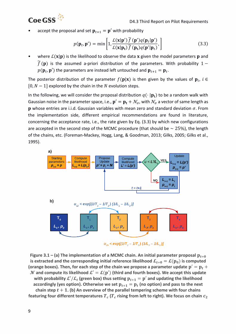
Figure 3.1 – (a) The implementation of a MCMC chain. An initial parameter proposal 𝐩𝒕=𝟎 is extracted and the corresponding initial reference likelihood 𝓛𝒕=𝟎 = 𝓛(𝐩𝟎) is computed

(orange boxes). Then, for each step of the chain we propose a parameter update 𝐩′ = 𝐩𝒕 +𝓝 and compute its likelihood 𝓛′ = 𝓛(𝐩′) (third and fourth boxes). We accept this update

with probability 𝓛′/𝓛𝒕 (green box) thus setting 𝐩𝒕+𝟏 = 𝐩′ and updating the likelihood accordingly (yes option). Otherwise we set 𝐩𝒕+𝟏 = 𝐩𝒕 (no option) and pass to the next

chain step 𝒕 + 𝟏. (b) An overview of the parallel tempering scheme with four chains featuring four different temperatures 𝑻𝒄 (𝑻𝒄 rising from left to right). We focus on chain 𝒄𝟐


10

that can exchange its configuration with the colder chain 𝒄𝟏 or with the hotter one 𝒄𝟑 with probabilities given in Eq. (3.4).

One of the issues frequently encountered in the MCMC model calibration is the number of

steps required for a chain to converge to the stationary distribution of 𝑓(𝐩|𝐱), which is usually

of the order of thousands of steps. This aspect is particularly relevant in large ABM simulations

that take several minutes to compute a single simulation of the system. When simulating such

systems, chains of MCMC integration cannot be made arbitrarily long while keeping the

constraint of having an acceptable computation time. That is why several methods to speed-

up the convergence of a chain have been put forward (Angelino, Kohler, Waterland, Seltzer,

& Adams, 2014; Brockwell, 2006; Earl & Deem, 2005; Foreman-Mackey et al., 2013; Goodman

& Weare, 2010; Swendsen & Wang, 1986; VanDerwerken & Schmidler, 2013).

All of these methods leverage on the parallel execution of different chains to improve the

exploration of a single chain or to better sample the parameter space. Among them, the

parallel tempering (Earl & Deem, 2005; Swendsen & Wang, 1986) implementation relies on 𝐶

MCMC chains running in parallel. The chains feature different “temperatures” 𝑇𝑐, i.e., the

proposed parameter update in each chain is computed using a different standard deviation

𝜎𝑐, with 𝑐 ∈ [1, 𝐶]. In other words, the size of the random “kick” given to the parameters’

values at each evolution step will be larger for larger values of 𝜎𝑐 that intuitively correspond

to higher temperatures as the system is able to explore more valleys of the 𝑓(𝐩|𝐱) posterior

distribution in fewer steps.

Each chain 𝑐 is then communicating with its two neighbours 𝑐 − 1 and 𝑐 + 1 to exchange their

parameter configurations 𝐩𝑐 with a probability depending on the score of the model ℒ(𝐱|𝐩𝐜)

and the temperature 𝑇𝑐 of the 𝑐-th and 𝑐 ± 1-th chains. Specifically, chain 𝑐 and 𝑐 + 1 will

switch their configuration if:

𝑢 < exp[(𝑇𝑐−1 − 𝑇𝑐+1

−1 )(ℒ𝑐−1 − ℒ𝑐+1

−1 )], (3.4)

where 𝑢 is a randomly generated number uniformly distributed in the [0,1) range, and ℒ𝑖 is

the likelihood of the model using the current parameter configuration of the 𝑖-th chain.

Stated differently, the hotter chains are responsible for an overall, fast exploration of the

parameter space. Once they find a well-performing region of parameters, they can propagate

their current configuration to the colder chains that will explore the proposed area in more

detail. A pictorial representation of this procedure is given in Fig. 3.1 (b).


11

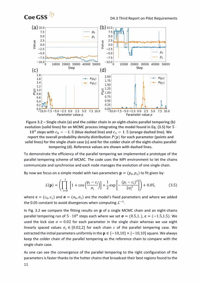
Figure 3.2 – Single chain (a) and the colder chain in an eight-chains parallel tempering (b) evolution (solid lines) for an MCMC process integrating the model found in Eq. (3.5) for 𝟓 ⋅

𝟏𝟎𝟒 steps with 𝒄𝟎 = −𝟏. 𝟓 (blue dashed line) and 𝒄𝟏 = 𝟏. 𝟓 (orange dashed line). We report the overall probability density distribution 𝑷(𝒑) for each parameter (points and

solid lines) for the single chain case (c) and for the colder chain of the eight-chains parallel tempering (d). Reference values are shown with dashed lines.

To demonstrate the efficiency of the parallel tempering we implemented a prototype of the

parallel tempering scheme of MCMC. The code uses the MPI environment to let the chains

communicate and synchronise and each node manages the evolution of one single chain.

By now we focus on a simple model with two parameters 𝐩 = (𝑝0, 𝑝1) to fit given by:

ℒ(𝐩) = (∏

1

𝑖=0

[1 + cos (𝑝𝑖 − 𝑐𝑖

𝜎𝑖)] +

1

2exp [−

(𝑝𝑖 − 𝑐𝑖)2

2𝜎𝑖2 ]) + 0.05, (3.5)

where 𝐜 = (𝑐0, 𝑐1) and 𝛔 = (𝜎0, 𝜎1) are the model’s fixed parameters and where we added

the 0.05 constant to avoid divergences when computing ℒ−1.

In Fig. 3.2 we compare the fitting results on 𝐩 of a single MCMC chain and an eight-chains

parallel tempering run of 5 ⋅ 104 steps each where we set 𝛔 = (0.5,1. ), 𝐜 = (−1.5,1.5). We

used the kick size 𝜎 = 0.02 for each parameter in the single chain whereas we use eight

linearly spaced values 𝜎𝑐 ∈ [0.02,2] for each chain 𝑐 of the parallel tempering case. We

extracted the initial parameters uniformly in the 𝐩 ∈ [−10,10] × [−10,10] square. We always

keep the colder chain of the parallel tempering as the reference chain to compare with the

single chain case.

As one can see the convergence of the parallel tempering to the right configuration of the

parameters is faster thanks to the hotter chains that broadcast their best regions found to the


12

colder, slower chains. On the other hand, the single chain slowly samples the parameter space

and it does not even find the correct parameter region even after 50 thousand evolution steps.

The model presented here is simple and runs in a few milliseconds on a single computing node

so that a parallel tempering implementation is straightforward. However, when fitting large

ABM models running on multiple nodes one problem to solve is the communication between

several multi-node processes running: communication can either be done via disk or with an

ad-hoc communication protocol in order to coordinate the chains’ exploration of the

parameter space.

Moreover, the necessity to run long chains to compute the posteriori distribution of the

model’s parameters highlights the importance of having a performing simulation framework

able to simulate long chains in an acceptable computation time, as well as a speedy

communication software and hardware infrastructure able to let the chains to quickly update

their status. To this end the co-design of a new simulation framework able to speed up

simulations and efficiently scale with the number of nodes is already set up between the pilots

and the HPC part.

Another crucial aspect, as detailed in the next section, is the design of an efficient online data

analysis to evaluate the likelihood of the simulated parameters, i.e. give a score to the

simulation just run as the MCMC approach requires it at every step to update the chains.

3.2 High-performance data analytics The class of agent-based models offers large freedom to the modeller in implementing various

dynamics. This benefit makes this approach very valuable to the GSS community and is one

reason for its popularity. However, this flexibility implies that the overall system behaviour is

hard to predict a priori. Specifically, for ABM it is often the goal to generate complex and partly

un-expected behaviour from the interaction of many agents. On a small scale, the modeller

often can explore this behaviour and derive necessary causal relationships. For high-

performance applications of agent-based models, the project identified an urgent need for

model analysis for GSS models within the development process. High-performance data

analytics (HDPA) is an emerging field in scientific computing that provides powerful tools for

data analysis on large amounts of distributed data.

Two approaches for model analysis can be envisioned:

• Online analysis: The model simulation itself aggregates and logs all important data that

is requested by the modeller to analyse a specific part of the model. This has the

advantage of using computing resources efficiently, especially in parallel

implementations. However, new and changing questions that need other aggregations

or output require changes in the model code or control parameters. After that the

simulation needs to be re-executed to generate the new data output. This approach

works well for mature models and rarely changing analysis questions.


13

• Offline (post processing) analysis: For this approach, all important data is stored during

the model run for later analysis, which is done by an analysis tool. Firstly, this allows using

well established software solutions, for example of the field of Big-Data analysis tools

(e.g., Spark). Secondly, the same model output can be analysed regarding several and

changing questions (which may not all be known at the time of the model execution)

without altering or re-executing the model. However, by offering more flexibility, this

approach also poses higher requirements in terms of data storage. This approach is

beneficial for often changing analysis questions that can be applied to all previously

generated model output.

In the following, we sketch the requirements for an offline analysis solution framework that

would optimally work together with the HPC-model application. We will focus on three

challenges: software solutions, hardware solutions, and user interface, which all three are

important to establish a useful scientific tool for the community of GSS-modellers.

3.2.1 Software Common Big-Data applications, like Spark and Hadoop and distributed data processing

libraries, like Dask, are potential candidates for post processing data analysis. Such analysis

comprises common statistical analysis tools (mean, variance, conditional mean, entropy...),

any kind of filter techniques, learning techniques like clustering, pattern recognition and

principal component analysis, and optimisation methods. Spark offers a separate graph

analysis toolbox with may be useful for analysing social graphs. Thus, Spark was chosen for

some initial tests which have been performed using output data from the Green Growth pilot’s

Mobility Transition Model (MoTMo, see D4.5). In these tests, existing post-processing queries

were implemented as Spark queries in a testing environment.

3.2.2 Hardware At the two HPC-centres in CoeGSS, Spark software is installed on a specific hardware

architecture, which means a different computing hardware. Thus, an offline-HDPA approach

using Spark would require the new hardware to have access to the model output. This means

there is a need for either copying the data to a second storage, or for a shared storage system.

The established HPC approach of an InfiniBand Lustre system (highly efficient storage for

parallel access of MPI-applications) is the most promising candidate, which is however only

optimised for MPI, not for HPDA. However, copying data between different storage hardware

would probably neglect most of the many performance increases that is provided by Big-Data

analysis. Thus, the Lustre file system should be accessible by both the HDPA and the HPC

system.

To estimate the storage requirements, we use the current output of the Green Growth pilot.

Currently one model run of MoTMo generates 320 GB of data. Of course, the amount of

output data depends on which subset of data from a model run is stored. Currently all the

properties of each agent are stored at each time step, which can be reduced at later stages.


14

Thus, we assume a reduction to 32 GB of relevant output might be a reasonable estimate for

the size of the output data. Assuming an ensemble of model runs that consists of 1000

realisations would require 32 TB of storage space, which is commonly provided by Lustre file

systems. Assuming several users are working in parallel would easily multiply required

storage. Since all data is analysed, the same fast access is required by the HDPA hardware as

by the HPC hardware, which might pose a challenge to the design of future computing clusters.

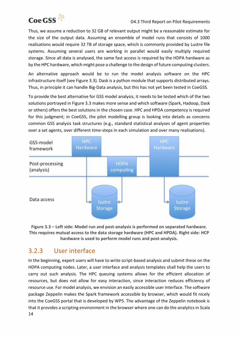
An alternative approach would be to run the model analysis software on the HPC

infrastructure itself (see Figure 3.3). Dask is a python module that supports distributed arrays.

Thus, in principle it can handle Big-Data analysis, but this has not yet been tested in CoeGSS.

To provide the best alternative for GSS model analysis, it needs to be tested which of the two

solutions portrayed in Figure 3.3 makes more sense and which software (Spark, Hadoop, Dask

or others) offers the best solutions in the chosen case. HPC and HPDA competency is required

for this judgment; in CoeGSS, the pilot modelling group is looking into details as concerns

common GSS analysis task structures (e.g., standard statistical analyses of agent properties

over a set agents, over different time-steps in each simulation and over many realisations).

Figure 3.3 – Left side: Model run and post-analysis is performed on separated hardware. This requires mutual access to the data storage hardware (HPC and HPDA). Right side: HCP

hardware is used to perform model runs and post-analysis.

3.2.3 User interface In the beginning, expert users will have to write script-based analysis and submit these on the

HDPA computing nodes. Later, a user interface and analysis templates shall help the users to

carry out such analysis. The HPC queuing systems allows for the efficient allocation of

resources, but does not allow for easy interaction, since interaction reduces efficiency of

resource use. For model analysis, we envision an easily accessible user interface. The software

package Zeppelin makes the Spark framework accessible by browser, which would fit nicely

into the CoeGSS portal that is developed by WP5. The advantage of the Zeppelin notebook is

that it provides a scripting environment in the browser where one can do the analytics in Scala


15

or Python. A big advantage would be to get built-in front-end support that is able to do very

nice plots and can make use of all sorts of graphical visualisation tools (Javascript, Python).

However, you do not get the full development support that a modern IDE provides.

3.3 Adaptive parameter space exploration We first justify the interest of adaptive parameter space exploration, before outlining more

specific requirements and proposing an existing tool.

3.3.1 Motivation There are many reasons why adaptive parameter space exploration can prove precious, going

from meeting specific Global System Science (GSS) needs to highlighting High Performance

Computing (HPC) strengths, while clearly outperforming plain parameter sweeps allowed by

the Cloud. Such adaptive parameter space explorations also highlight synergies between GSS

and HPC. We detail these motivations in the following paragraphs.

3.3.1.1 Why parameter space exploration is important in Global System Science modelling

Exploring the behaviour of a model over the parameter space is essential in Global Systems

Science, firstly when designing and validating the model and secondly when running it once

validated.

Firstly, the complexity of the reality to simulate requests a certain level of model complexity

involving many parameters while still remaining simpler than the reality. Tailoring as precisely

as possible the model to a specific modelling need, therefore often requires a few cycles of

model refinement and validation. Key phases of such a cycle, including calibration and

validation, require to explore the model behaviour as thoroughly as possible over the

parameter space – and not just to run a limited set of simulations giving an incomplete view

of the model behaviour.

Secondly, once validated, GSS models can be used for decision support, their parameters

corresponding to possible political leverage (level of information, incentives, ...), and their

observables corresponding to the value of key performance indicators (citizen happiness,

number of smokers, pollution, real estate prices, revenue, ...).

Therefore, they might require: firstly, to predict possible outcomes, to simulate many possible

scenarios, possibly over continuous parameter values, while observing non-trivially evolving

key performance indicators. Secondly, to prescribe desirable outcomes, they might require

further simulations to find out for instance how to optimise some key performance indicators,

or to evaluate tipping points or areas (e.g. predominance of green cars following the level of

some incentive), or else to assess risk or benefit zones (for instance high or low levels of

smokers).


16

3.3.1.2 Why prefer adaptive parameter space exploration to systematic parameter sweep?

Adaptive parameter space exploration allows to optimise the choice of simulations following

the purpose of the study. Its benefit is multi-fold.

• Avoid and limit unnecessary simulations and thereby optimise computation time use.

• Increase accuracy of the results finally obtained, with a similar (or lower) number of

simulations.

• Detect and describe automatically areas of interest, without requesting a priori

assumptions, leading to possibly new discoveries.

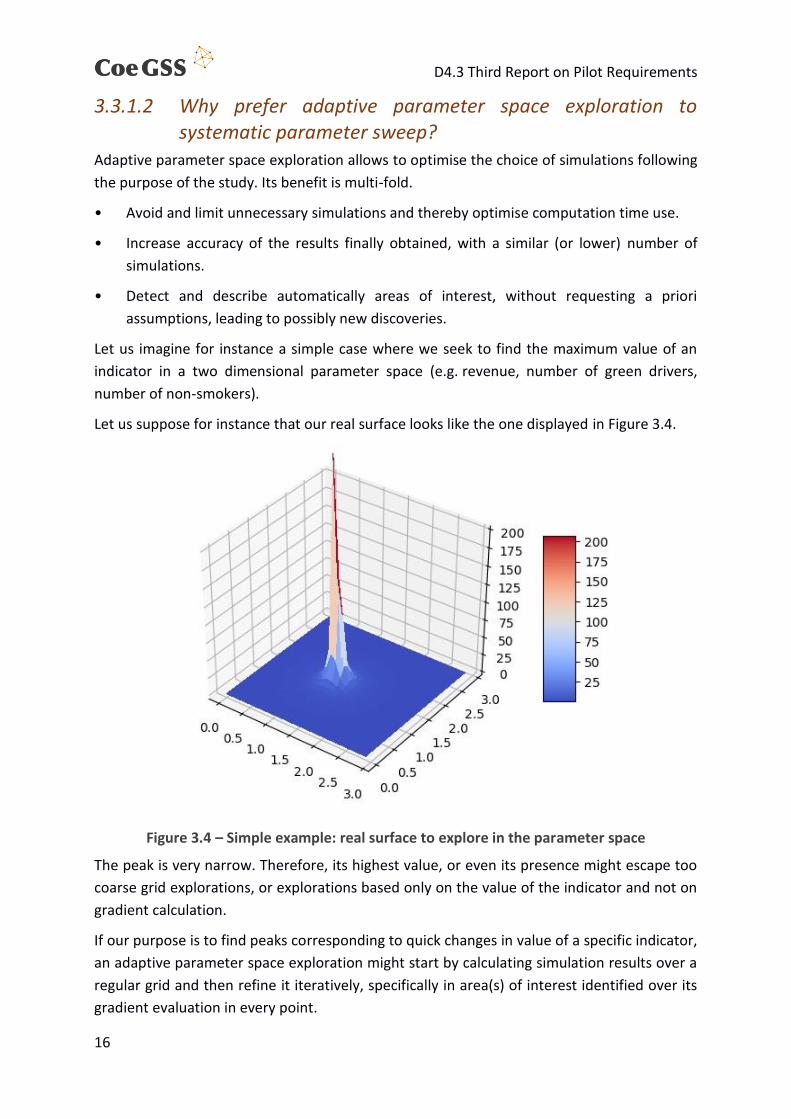
Let us imagine for instance a simple case where we seek to find the maximum value of an

indicator in a two dimensional parameter space (e.g. revenue, number of green drivers,

number of non-smokers).

Let us suppose for instance that our real surface looks like the one displayed in Figure 3.4.

Figure 3.4 – Simple example: real surface to explore in the parameter space

The peak is very narrow. Therefore, its highest value, or even its presence might escape too

coarse grid explorations, or explorations based only on the value of the indicator and not on

gradient calculation.

If our purpose is to find peaks corresponding to quick changes in value of a specific indicator,

an adaptive parameter space exploration might start by calculating simulation results over a

regular grid and then refine it iteratively, specifically in area(s) of interest identified over its

gradient evaluation in every point.


17

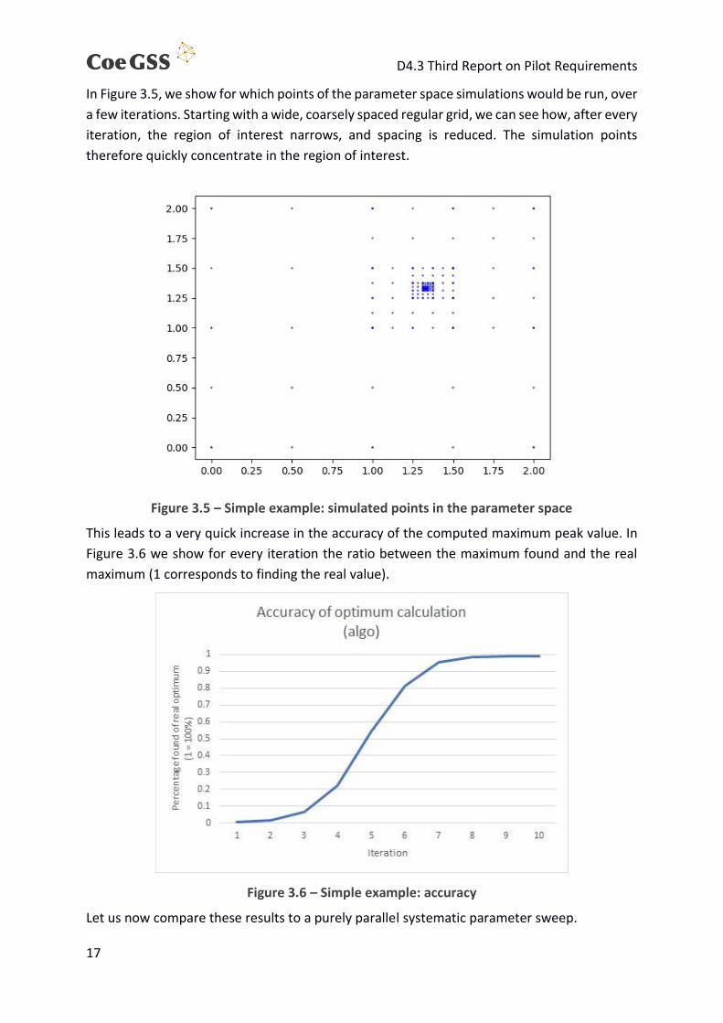
In Figure 3.5, we show for which points of the parameter space simulations would be run, over

a few iterations. Starting with a wide, coarsely spaced regular grid, we can see how, after every

iteration, the region of interest narrows, and spacing is reduced. The simulation points

therefore quickly concentrate in the region of interest.

Figure 3.5 – Simple example: simulated points in the parameter space

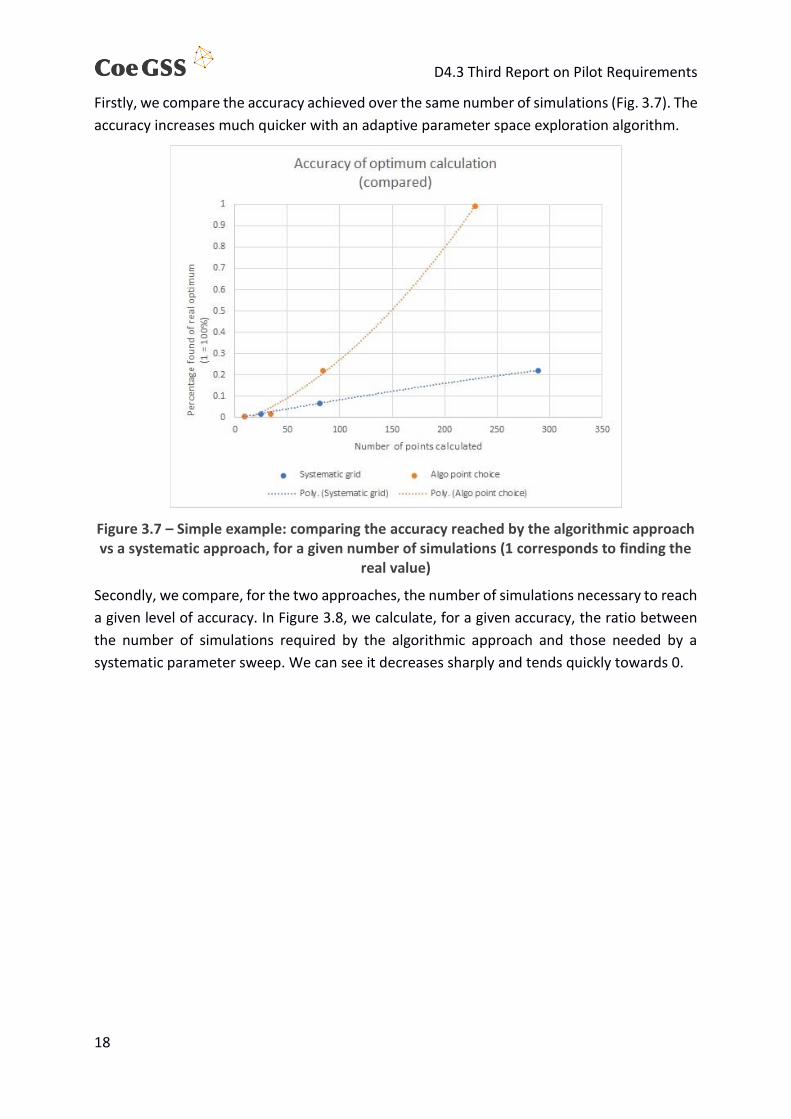
This leads to a very quick increase in the accuracy of the computed maximum peak value. In

Figure 3.6 we show for every iteration the ratio between the maximum found and the real

maximum (1 corresponds to finding the real value).

Figure 3.6 – Simple example: accuracy

Let us now compare these results to a purely parallel systematic parameter sweep.


18

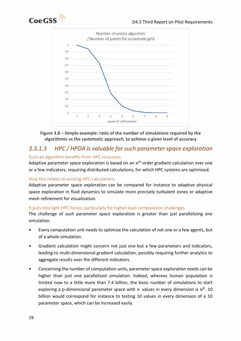
Firstly, we compare the accuracy achieved over the same number of simulations (Fig. 3.7). The

accuracy increases much quicker with an adaptive parameter space exploration algorithm.

Figure 3.7 – Simple example: comparing the accuracy reached by the algorithmic approach vs a systematic approach, for a given number of simulations (1 corresponds to finding the

real value)

Secondly, we compare, for the two approaches, the number of simulations necessary to reach

a given level of accuracy. In Figure 3.8, we calculate, for a given accuracy, the ratio between

the number of simulations required by the algorithmic approach and those needed by a

systematic parameter sweep. We can see it decreases sharply and tends quickly towards 0.


19

Figure 3.8 – Simple example: ratio of the number of simulations required by the algorithmic vs the systematic approach, to achieve a given level of accuracy

3.3.1.3 HPC / HPDA is valuable for such parameter space exploration Such an algorithm benefits from HPC resources Adaptive parameter space exploration is based on an nth order gradient calculation over one

or a few indicators, requiring distributed calculations, for which HPC systems are optimised.

How this relates to existing HPC calculations Adaptive parameter space exploration can be compared for instance to adaptive physical

space exploration in fluid dynamics to simulate more precisely turbulent zones or adaptive

mesh refinement for visualisation.

It puts into light HPC forces, particularly for higher level computation challenges The challenge of such parameter space exploration is greater than just parallelizing one

simulation.

• Every computation unit needs to optimise the calculation of not one or a few agents, but

of a whole simulation.

• Gradient calculation might concern not just one but a few parameters and indicators,

leading to multi-dimensional gradient calculation, possibly requiring further analytics to

aggregate results over the different indicators.

• Concerning the number of computation units, parameter space exploration needs can be

higher than just one parallelised simulation. Indeed, whereas human population is

limited now to a little more than 7.4 billion, the basic number of simulations to start

exploring a p-dimensional parameter space with 𝑛 values in every dimension is 𝑛𝑝. 10

billion would correspond for instance to testing 10 values in every dimension of a 10

parameter space, which can be increased easily.


20

• Increasing the number of nodes should allow to scale up easily, adding only localised

inter-node communications. In contrast, when parallelizing a single GSS simulation and

dispatching agents over nodes, increasing the number of agents in a highly

interconnected population can require to increase quadratically the number of inter-

node communications.

3.3.1.4 Adaptive parameter space exploration highlights GSS-HPC synergies in CoeGSS

Here are a few possible benefits

• Bridging a specific GSS need (parameter space exploration) with specific HPC strengths

(enhanced inter-node communications optimizing gradient calculations essential to

adaptive parameter space exploration).

• HPC resources, by enhancing this kind of adaptive space exploration, open to more

efficient and thorough space exploration in a given time while not limiting such

explorations to explicitly defined areas of interest, hopefully allowing therefore for new

GSS discoveries.

• These specific GSS needs, by proposing new challenges for HPC, concerning both the

work load per calculation unit, the number of necessary units and their required

communications, hopefully will allow to put further into light HPC strengths.

3.3.2 More detail on needs and requirements The GSS scope being very wide, it is difficult to provide requirements defining limited needs,

as for instance fluid dynamics limited to a 3 (or 4 including time) dimensional space.

3.3.2.1 Parameter space characterisation There is no limitation on the kind of parameter space to be explored. Parameters of interest

may concern any part of the model, thematically, but also at different scales, for instance

• Global ones, corresponding to one value, such as shared level of overall information,

global incentives, ...

• Individual ones corresponding to possible distributions, themselves characterised by a

few parameters defining for instance a random distribution (average, standard deviation,

...), such as a level of ecological awareness or income.

In any case there is no limit on their number or kind.

Therefore, tools are required to allow for space exploration with as many dimensions as

possible (and multi-dimensional gradient calculation).


21

3.3.2.2 Indicator(s) characterisation Here again many indicators can be simultaneously of interest, either as direct output of

simulations, or calculated therefrom. Further they might be of different kinds (discrete,

continuous ...)

Therefore, tools are required to allow calculating (multi-dimensional) gradients over a few

indicators, while providing analytical tools.

3.3.2.3 Exploration target(s) There can be various purposes for such a parameter space exploration, targeting different

kinds of areas of interest and requiring various kinds of gradient or other analytics calculations.

Tools should allow to answer such needs.

Exploration purpose Purposes of such an exploration include

• Calibration

• Validation

• Finding an optimum

• Finding the conditions of a change in behaviours (e.g., predominating behaviour, level of

pollution)

• Defining areas of risk or benefit (resiliency)

Areas of interest Areas of interest which tools should allow to target are

• Points: finding an optimum (ex. happiness, green spirit, income)

• Lines: defining tipping lines from one kind of outcome to another (green behaviour or

non-smoking prevailing)

• Surfaces: risk or benefit areas: too high pollution, resiliency,

Which kind of gradient calculation? Necessary calculations concern

• Simple value

• First order gradient to detect quick changes in value

• Second order gradient to detect optima

Other analytics? These calculations are likely to require the further calculation of analytics, for instance to

aggregate information over various observables into a single indicator. Any tool should also

allow for such intermediate calculations.


22

3.3.3 Existing solutions

3.3.3.1 Algorithms and approaches See corresponding section in D4.5.

3.3.3.2 HPC-oriented software Dakota (https://dakota.sandia.gov/), A Multilevel Parallel Object-Oriented Framework for

Design Optimisation, Parameter Estimation, Uncertainty Quantification, and Sensitivity

Analysis provides such facilities while being developed for running on HPC.


23

4 Next steps This document provides the last iteration of the deliverable that reports on pilot requirements

to the Centre of Excellence for Global Systems Science. Complementing D4.1 and D4.2, it has

focused on the simulation part in the work on a GSS-SIS, by specifying requirements for easy

access to the computing resources and for different simulation analysis techniques.

However, the deliverable is neither exhaustive nor does it represent the final word on GSS

requirements to HPC within the project, where the requirements presented here will be

further discussed and refined within some of the working groups as needed. Requirements

stated in the previous iterations remain valid, without having been repeated here, for

example, those on data collection and pre-processing, on an ABM framework and on

visualisation.

Further work on using the techniques presented in Section 3 shall be carried out by the three

pilots, with a special focus of the Health Habits pilot on Markov Chain Monte Carlo

applications, of the Green Growth pilot on high performance data analytics tools, and of the

Global Urbanisation pilot on adaptive parameter space exploration.


24

5 References

5.1 CoeGSS Deliverables D2.2: CoeGSS Deliverable D2.2; INTERMEDIATE SUSTAINABILITY MODEL; to be delivered to

the European Commission; Franziska Schütze, Blanca Jordan (editors), Leonardo Camiciotti,

Nigina Abdullaeva, Sarah Wolf, Steffen Fürst, Andreas Geiges, Eva Richter, Bastian Koller

D4.1: CoeGSS Deliverable D4.1; FIRST REPORT ON PILOT REQUIREMENTS; delivered to the

European Commission; Sarah Wolf (editor), Daniela Paolotti, Michele Tizzoni, Margaret

Edwards, Steffen Fürst, Andreas Geiges, Alfred Ireland, Franziska Schütze, Gesine Steudle

D4.2: CoeGSS Deliverable D4.2; SECOND REPORT ON PILOT REQUIREMENTS; delivered to the

European Commission; Sarah Wolf (editor), Margaret Edwards, Steffen Fürst, Andreas

Geiges, Luca Rossi, Michele Tizzoni, Enrico Ubaldi

D4.4: CoeGSS Deliverable D4.4; FIRST STATUS REPORT OF THE PILOTS; delivered to the

European Commission; Sarah Wolf (editor), Marion Dreyer, Margaret Edwards, Steffen Fürst,

Andreas Geiges, Jörg Hilpert, Jette von Postel, Fabio Saracco, Michele Tizzoni, Enrico Ubaldi

D4.5: CoeGSS Deliverable D4.5; SECOND STATUS REPORT OF THE PILOTS; delivered to the European Commission; Sarah Wolf (editor), Andreas Geiges, Steffen Fürst, Enrico Ubaldi, Margaret Edwards, Jette von Postel

5.2 Literature Angelino, E., Kohler, E., Waterland, A., Seltzer, M., & Adams, R. P. (2014). Accelerating

MCMC via parallel predictive prefetching. arXiv Preprint arXiv:1403.7265.

Brockwell, A. E. (2006). Parallel Markov Chain Monte Carlo simulation by pre-fetching.

Journal of Computational and Graphical Statistics, 15(1), 246–261.

Earl, D. J., & Deem, M. W. (2005). Parallel tempering: Theory, applications, and new

perspectives. Physical Chemistry Chemical Physics, 7(23), 3910–3916.

Foreman-Mackey, D., Hogg, D. W., Lang, D., & Goodman, J. (2013). Emcee: The MCMC

hammer. Publications of the Astronomical Society of the Pacific, 125(925), 306.

Gilks, W. R. (2005). Markov Chain Monte Carlo. Encyclopedia of Biostatistics.

Gilks, W. R., Richardson, S., & Spiegelhalter, D. (1995). Markov Chain Monte Carlo in practice.

CRC press.

Goodman, J., & Weare, J. (2010). Ensemble samplers with affine invariance. Communications

in Applied Mathematics and Computational Science, 5(1), 65–80.

Swendsen, R. H., & Wang, J.-S. (1986). Replica Monte Carlo simulation of spin-glasses.

Physical Review Letters, 57(21), 2607.


25

VanDerwerken, D. N., & Schmidler, S. C. (2013). Parallel Markov Chain Monte Carlo. arXiv

Preprint arXiv:1312.7479.

Appendix A

Green Growth pilot workflow description (from the project internal wiki)

This workflow was used for the global model implemented for the Green Growth pilot, details

on the model can be found in D4.4 and D4.5.

Documents

D4.3 THIRD REPORT ON PILOT REQUIREMENTScoegss.eu/wp-content/uploads/2018/02/D4.3.pdf · D4.3 Third Report on Pilot Requirements 5 List of Figures Figure 3.1 – The implementation