Embed Size (px)
Citation preview
ICT-287510RELEASE
A High-Level Paradigm for Reliable Large-Scale Server SoftwareA Specific Targeted Research Project (STReP)
D3.4 (WP3): Scalable Reliable OTP Library Release:
Patterns for Scaling Distributed Erlang Applications
Due date of deliverable: 31st August 2014Actual submission date: 23rd September 2014
Start date of project: 1st October 2011 Duration: 41 months
Lead contractor: The University of Glasgow Revision: 1.0
Purpose: Design, implement and validate a set of reusable reliable massively parallel programmingpatterns as a scalable, performance portable OTP library.
Results: The main results of this deliverable are as follows.
� We have discussed scalability recipes of distributed Erlang applications using four benchmarks.
� We have provided scalability and reliability principles, application methodology, and introducedgeneric patterns.
� We have briefly outlined performance portability under development for deliverable D3.5.
Conclusion: We have identified generic patterns, introduced methodology for scalable reliable SDErlang applications, and both designed and implemented them in a number of SD Erlang benchmarks.
Project funded under the European Community Framework 7 Programme (2011-14)Dissemination Level
PU Public >PP Restricted to other programme participants (including the Commission Services)RE Restricted to a group specified by the consortium (including the Commission Services)CO Confidential only for members of the consortium (including the Commission Services)
ICT-287510 (RELEASE) 23rd September 2014 1
Scalable Reliable OTP Library Release: Patterns for Scaling DistributedErlang Applications
Contents
1 Introduction 2
2 SD Erlang Overview 3
3 Recipes for Scalability of Distributed Erlang Applications 33.1 Orbit (P2P) . . . . . . . . . . . . . . . . . . . . . . . . . . . . . . . . . . . . . . . . . . . 43.2 Ant Colony Optimisation (Master-Slave) . . . . . . . . . . . . . . . . . . . . . . . . . . . 83.3 Instant Messenger (Server) . . . . . . . . . . . . . . . . . . . . . . . . . . . . . . . . . . 133.4 Sim-Diasca (Multicomponent) . . . . . . . . . . . . . . . . . . . . . . . . . . . . . . . . . 153.5 Summary . . . . . . . . . . . . . . . . . . . . . . . . . . . . . . . . . . . . . . . . . . . . 18
4 Distributed Erlang Scalability Principles & Application Methodology 184.1 Replacing All-to-all Connections . . . . . . . . . . . . . . . . . . . . . . . . . . . . . . . 18
4.1.1 Issues with All-to-all Connections. . . . . . . . . . . . . . . . . . . . . . . . . . . 184.1.2 Ad Hoc Approaches . . . . . . . . . . . . . . . . . . . . . . . . . . . . . . . . . . 194.1.3 RELEASE Approach: s groups . . . . . . . . . . . . . . . . . . . . . . . . . . . . 194.1.4 Functions to Group Nodes . . . . . . . . . . . . . . . . . . . . . . . . . . . . . . . 20
4.2 Replacing Global Namespace . . . . . . . . . . . . . . . . . . . . . . . . . . . . . . . . . 234.3 Eliminating Single Process Bottleneck . . . . . . . . . . . . . . . . . . . . . . . . . . . . 24
5 Reliability Principles 25
6 Performance Portability 26
7 Implications and Future Work 29
A Notes on Ant Colony Optimisation in Erlang 31A.1 The Single Machine Total Weighted Tardiness Problem . . . . . . . . . . . . . . . . . . 31
A.1.1 Example data for the SMTWTP. . . . . . . . . . . . . . . . . . . . . . . . . . . . 31A.2 Ant Colony Optimisation . . . . . . . . . . . . . . . . . . . . . . . . . . . . . . . . . . . 32
A.2.1 Overview . . . . . . . . . . . . . . . . . . . . . . . . . . . . . . . . . . . . . . . . 32A.2.2 Application to the SMTWTP. . . . . . . . . . . . . . . . . . . . . . . . . . . . . . 32
A.3 Implementation in Erlang (Single Machine) . . . . . . . . . . . . . . . . . . . . . . . . . 34A.3.1 Difficulties with Erlang . . . . . . . . . . . . . . . . . . . . . . . . . . . . . . . . 35A.3.2 Behaviour . . . . . . . . . . . . . . . . . . . . . . . . . . . . . . . . . . . . . . . . 35
A.4 Distributed ACO techniques . . . . . . . . . . . . . . . . . . . . . . . . . . . . . . . . . . 36A.4.1 Implementation strategy . . . . . . . . . . . . . . . . . . . . . . . . . . . . . . . . 36
A.5 Measuring Scalability . . . . . . . . . . . . . . . . . . . . . . . . . . . . . . . . . . . . . 37
ICT-287510 (RELEASE) 23rd September 2014 2
B ACO Performance 38B.1 Performance of SMP version of ACO application . . . . . . . . . . . . . . . . . . . . . . 38B.2 Experiments: ETS . . . . . . . . . . . . . . . . . . . . . . . . . . . . . . . . . . . . . . . 39B.3 Experiments: DETS . . . . . . . . . . . . . . . . . . . . . . . . . . . . . . . . . . . . . . 41B.4 Comparing ETS and DETS . . . . . . . . . . . . . . . . . . . . . . . . . . . . . . . . . . 43
Executive Summary
In this deliverable we discuss methodology and patterns for building SD Erlang applications, as wellas our plans to extend the s group.erl module in the RELEASE branch of Erlang/OTP. The work isclosely related to the work in WP5 on refactoring and tuning SD Erlang applications, in particular todeliverables D5.3: Systematic Testing and Debugging Tools and D5.4: Interactive SD Erlang Debugger.
The discussion and methodologies we provide in this deliverable are derived from the followingfour benchmarks of different types: Orbit (P2P), Ant Colony Optimisation (master/slave), InstantMessenger (server), and Sim-Diasca (multicomponent) (Section 3). We start with non-distributedErlang versions of the applications and then refactor them first into distributed Erlang, and then intoSD Erlang. This is done to show differences between the familiar non-distributed Erlang → distributedErlang refactoring and the new distributed Erlang → SD Erlang refactoring. Using the observationsfrom the benchmarks we discuss scalability principles of distributed Erlang applications (Section 4). Wedo not aim to cover scalability issues related to a single Erlang node (the single node scalability issuesare discussed and dealt with in WP2 deliverables) but rather focus on scalability features of distributedapplications and SD Erlang. These are replacing all-to-all connections, grouping nodes, replacing globalnamespaces, and eliminating single process bottlenecks. We also discuss reliability features of SD Erlang(Section 5) and briefly cover our ongoing work on portability principles (Section 6).
The reliable SD Erlang is open source and can be found in Github https://github.com/release
-project/otp/tree/dev.
1 Introduction
The objectives of Task 3.4 are to “design, implement and validate a set of reusable Reliable MassivelyParallel (RMP) programming patterns as a scalable, performance portable OTP library”. The leadparticipant is the University of Glasgow.
The aim of this deliverable is to demonstrate approaches to scale distributed Erlang applications,and introduce application methodology and generic patterns. We start with an overview of SD Er-lang (Section 2). We then provide design and refactoring techniques of four benchmarks (Section 3)and discuss scalability principles and application methodology for SD Erlang applications (Section 4).These two sections are mutually complementary, that is we first started with benchmarks, derivedrefactoring techniques, formalised and improved those techniques, and then we applied them back tothe benchmarks. Then we discuss SD Erlang reliability features using Instant Messenger benchmarkas an example (Section 5). We provide our initial measurements and findings on performance porta-bility that will be further discussed in deliverable D3.5: SD Erlang Performance Portability Principles(Section 6). Finally, we summarise the deliverable and discuss our future plans (Section 7).
Partner Contributions to D3.4 We had a series of email exchange with the University of Kentand Erlang Solutions. The University of Kent contributed to the refactoring and tuning aspects of thebenchmarks, and together with the Erlang Solutions and Ericsson teams contributed to identifying thesimplest and the most efficient ways to install SD Erlang. All partners contributed to different aspectsof Sim-Diasca scaling.
ICT-287510 (RELEASE) 23rd September 2014 3
2 SD Erlang Overview
SD Erlang is a modest conservative extension of distributed Erlang [REL13a]. Its scalable computationmodel has two aspects: s groups and semi-explicit placement.
The reasons we have introduced s groups are to reduce the number of connections a node maintains,and reduce the size of namespaces. A namespace is a set of names replicated on a group of nodes andtreated as global in that group. In SD Erlang node connections and namespace are defined by boththe node belonging to an s group and by the node type, i.e. hidden or normal. If a node is freethat is it belongs to no s group, the connections and namespace only depend on the node type. Afree normal node has transitive connections and common namespace with all other free normal nodes.A free hidden node has non-transitive connections with all other nodes and every hidden node hasits own namespace. An s group node has transitive connections with nodes from the same s groupand non-transitive connections with other nodes. It may belong to a number of s groups. The SDErlang s groups are similar to the distributed Erlang hidden global groups in the following: (1) eachs group has its own namespace; (2) transitive connections are only with nodes of the same s group.The differences with hidden global groups are in that (1) a node can belong to an unlimited numberof s groups, and (2) information about s groups and nodes is not globally collected and shared. In SDErlang behaviour and functionality of free nodes remains the same as in distributed Erlang.
The semi-explicit and architecture aware process placement mechanism was introduced to enableperformance portability, a crucial mechanism in the presence of fast-evolving architectures (Section 6).
3 Recipes for Scalability of Distributed Erlang Applications
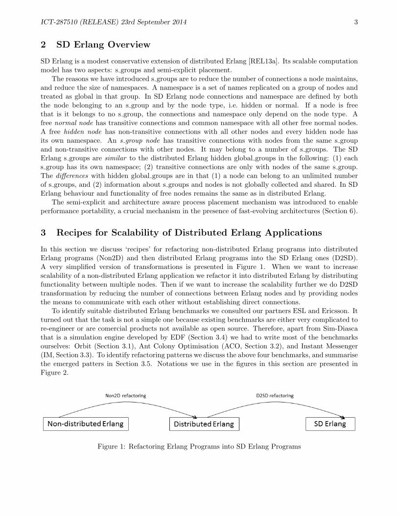
In this section we discuss ‘recipes’ for refactoring non-distributed Erlang programs into distributedErlang programs (Non2D) and then distributed Erlang programs into the SD Erlang ones (D2SD).A very simplified version of transformations is presented in Figure 1. When we want to increasescalability of a non-distributed Erlang application we refactor it into distributed Erlang by distributingfunctionality between multiple nodes. Then if we want to increase the scalability further we do D2SDtransformation by reducing the number of connections between Erlang nodes and by providing nodesthe means to communicate with each other without establishing direct connections.
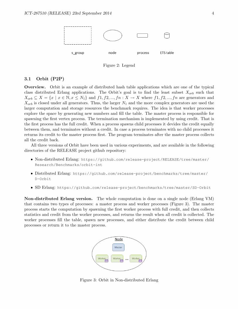
To identify suitable distributed Erlang benchmarks we consulted our partners ESL and Ericsson. Itturned out that the task is not a simple one because existing benchmarks are either very complicated tore-engineer or are comercial products not available as open source. Therefore, apart from Sim-Diascathat is a simulation engine developed by EDF (Section 3.4) we had to write most of the benchmarksourselves: Orbit (Section 3.1), Ant Colony Optimisation (ACO, Section 3.2), and Instant Messenger(IM, Section 3.3). To identify refactoring patterns we discuss the above four benchmarks, and summarisethe emerged patters in Section 3.5. Notations we use in the figures in this section are presented inFigure 2.
Figure 1: Refactoring Erlang Programs into SD Erlang Programs
ICT-287510 (RELEASE) 23rd September 2014 4
Figure 2: Legend
3.1 Orbit (P2P)
Overview. Orbit is an example of distributed hash table applications which are one of the typicalclass distributed Erlang applications. The Orbit’s goal is to find the least subset Xorb such thatXorb ⊆ X = {x | x ∈ N, x ≤ N1} and f1, f2, ..., fn : X → X where f1, f2, ..., fn are generators andXorb is closed under all generators. Thus, the larger N1 and the more complex generators are used thelarger computation and storage resources the benchmark requires. The idea is that worker processesexplore the space by generating new numbers and fill the table. The master process is responsible forspawning the first vertex process. The termination mechanism is implemented by using credit. That isthe first process has the full credit. When a process spawns child processes it devides the credit equallybetween them, and terminates without a credit. In case a process terminates with no child processes itreturns its credit to the master process first. The program terminates after the master process collectsall the credit back.
All three versions of Orbit have been used in various experiments, and are available in the followingdirectories of the RELEASE project github repository:
� Non-distributed Erlang: https://github.com/release-project/RELEASE/tree/master/Research/Benchmarks/orbit-int
� Distributed Erlang: https://github.com/release-project/benchmarks/tree/master/D-Orbit
� SD Erlang: https://github.com/release-project/benchmarks/tree/master/SD-Orbit
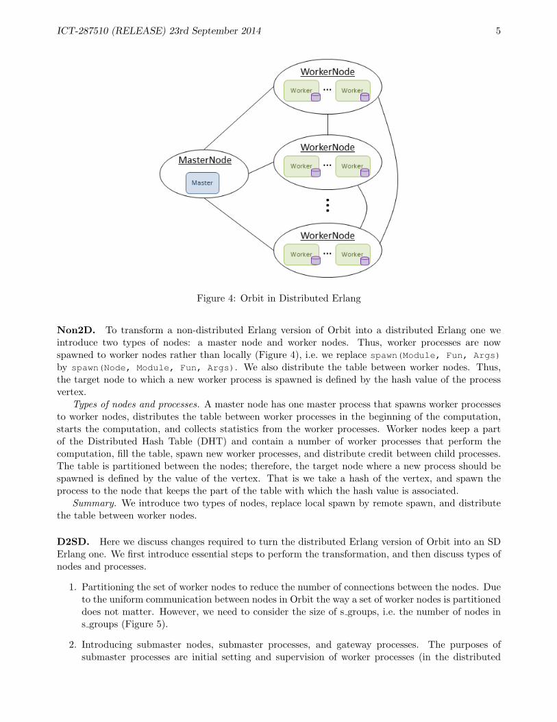
Non-distributed Erlang version. The whole computation is done on a single node (Erlang VM)that contains two types of processes: a master process and worker processes (Figure 3). The masterprocess starts the computation by spawning the first worker process with full credit, and then collectsstatistics and credit from the worker processes, and returns the result when all credit is collected. Theworker processes fill the table, spawn new processes, and either distribute the credit between childprocesses or return it to the master process.
Figure 3: Orbit in Non-distributed Erlang
ICT-287510 (RELEASE) 23rd September 2014 5
Figure 4: Orbit in Distributed Erlang
Non2D. To transform a non-distributed Erlang version of Orbit into a distributed Erlang one weintroduce two types of nodes: a master node and worker nodes. Thus, worker processes are nowspawned to worker nodes rather than locally (Figure 4), i.e. we replace spawn(Module, Fun, Args)
by spawn(Node, Module, Fun, Args). We also distribute the table between worker nodes. Thus,the target node to which a new worker process is spawned is defined by the hash value of the processvertex.
Types of nodes and processes. A master node has one master process that spawns worker processesto worker nodes, distributes the table between worker processes in the beginning of the computation,starts the computation, and collects statistics from the worker processes. Worker nodes keep a partof the Distributed Hash Table (DHT) and contain a number of worker processes that perform thecomputation, fill the table, spawn new worker processes, and distribute credit between child processes.The table is partitioned between the nodes; therefore, the target node where a new process should bespawned is defined by the value of the vertex. That is we take a hash of the vertex, and spawn theprocess to the node that keeps the part of the table with which the hash value is associated.
Summary. We introduce two types of nodes, replace local spawn by remote spawn, and distributethe table between worker nodes.
D2SD. Here we discuss changes required to turn the distributed Erlang version of Orbit into an SDErlang one. We first introduce essential steps to perform the transformation, and then discuss types ofnodes and processes.
1. Partitioning the set of worker nodes to reduce the number of connections between the nodes. Dueto the uniform communication between nodes in Orbit the way a set of worker nodes is partitioneddoes not matter. However, we need to consider the size of s groups, i.e. the number of nodes ins groups (Figure 5).
2. Introducing submaster nodes, submaster processes, and gateway processes. The purposes ofsubmaster processes are initial setting and supervision of worker processes (in the distributed
ICT-287510 (RELEASE) 23rd September 2014 6
Erlang implementation the worker processes are supervised by the master process). The gatewayprocesses act as routers. The submaster nodes only contain submaster and gateway processes.We have separated them for the benchmarking purpose; however, in general it may not be neededto keep submaster and gateway processes separately from worker processes.
3. Creating a submaster s group. The submaster s group contains the master node and all submasternodes.
4. Hierarchical process spawning. The master process spawns submaster and gateway processesto submaster nodes. Every submaster node has one submaster process, whereas the number ofgateway processes should be proportional to the following parameters to avoid gateway processbottleneck and resource wasting:
� the number of worker processes on the worker nodes.
� the number of nodes in the current s group.
� the number of s groups.
In turn submaster processes spawn worker processes to worker nodes. As before the target workernode is defined by the hash value of the worker process vertex.
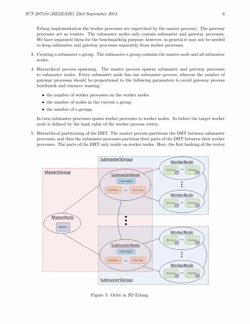
5. Hierarchical partitioning of the DHT. The master process partitions the DHT between submasterprocesses, and then the submaster processes partition their parts of the DHT between their workerprocesses. The parts of the DHT only reside on worker nodes. Here, the first hashing of the vertex
Figure 5: Orbit in SD Erlang
ICT-287510 (RELEASE) 23rd September 2014 7
defines the subgroup, and the second hashing defines the node to which a new process should bespawned.
6. Indirect communication between nodes from different s groups. The node to which a workerprocess spawns a new process is defined by the value of the vertex, i.e. the first hash of the vertexdefines the s group, and the second hash of the vertex defines the node. Thus, if both the initialand the target nodes are in the same s group then the process is spawned directly to the targetnode; otherwise the message is sent to a gateway process on the submaster node in the currents group (GT1), then GT1 forwards the message to a gateway process on the submaster node ofthe target s group (GT2), and then GT2 spawns a process to the target node.
7. Hierarchical information collection. The worker processes return the credit to their submasterprocesses, and then submaster processes return the credit to the master process.
Types of nodes and processes. A master node has one master process that starts the computationand collects statistics from submaster processes. The master process also spawns submaster processesand gateway processes. Every submaster node contains a single submaster process and a number ofgateway processes. The submaster processes distribute DHT to worker processes in the beginningof the computation, spawn worker processes, and collect statics from the worker processes. Gatewayprocesses forward messages between worker processes from different s groups. Worker nodes keep DHTsand contain a number of worker processes that perform the computation and fill the table, spawn newworker processes, and distribute credit between child processes.
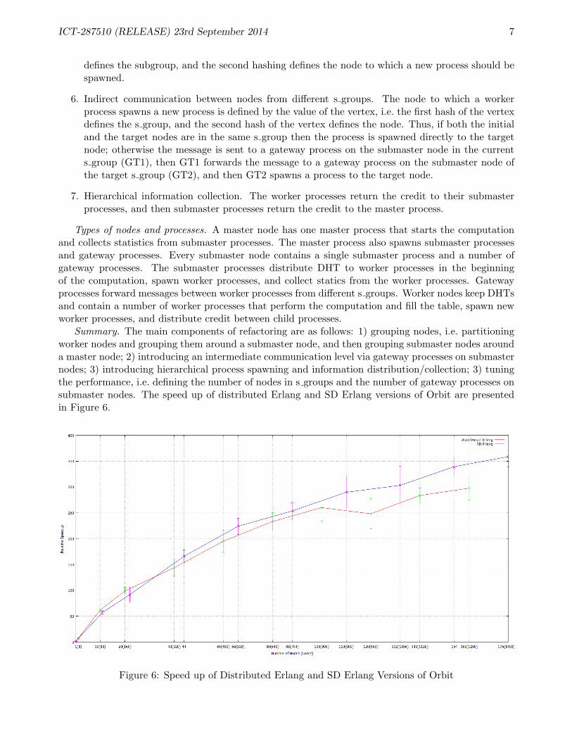
Summary. The main components of refactoring are as follows: 1) grouping nodes, i.e. partitioningworker nodes and grouping them around a submaster node, and then grouping submaster nodes arounda master node; 2) introducing an intermediate communication level via gateway processes on submasternodes; 3) introducing hierarchical process spawning and information distribution/collection; 3) tuningthe performance, i.e. defining the number of nodes in s groups and the number of gateway processes onsubmaster nodes. The speed up of distributed Erlang and SD Erlang versions of Orbit are presentedin Figure 6.
Figure 6: Speed up of Distributed Erlang and SD Erlang Versions of Orbit
ICT-287510 (RELEASE) 23rd September 2014 8
3.2 Ant Colony Optimisation (Master-Slave)
Ant Colony Optimisation (ACO) is a “metaheuristic” which has proved to be successful in a number ofdifficult combinatorial optimisation problems, including the Travelling Salesman, Vehicle Routing, andQuadratic Assignment problems. A detailed description of the method and its applications can be foundin the book [DS04]1; a more recent overview can be found in [DS10]. There is a vast amount of researchon this subject: an online bibliography at http://www.hant.li.univ-tours.fr/artantbib/artantbib.php currently has 1089 entries.
The ACO method is inspired by the behaviour of real ant colonies. Ants leave their colonies andgo foraging for food. The paths followed by ants are initially random, but when an ant finds somefood it will return to its home, laying down a trail of chemicals called pheromones which are attractiveto other ants. Other ants will then tend to follow the path to the food source. There will still berandom fluctuations in the paths followed by individual ants, and some of these may be shorter thanthe original path. Pheromones evaporate over time, which means that longer paths will become lessattractive while shorter ones become more attractive. This behaviour means that ants can very quicklyconverge upon an efficient path to the food source.
This phenomenon has inspired the ACO methodology for difficult optimisation problems. Thebasic idea is that a (typically very large) search space is explored by a number of artificial ants, eachof which makes a number of random choices to construct its own solution. The ants may also makeuse of heuristic information tailored to the specific problem. Individual solutions are compared, andinformation is saved in a structure called the pheromone matrix which records which records the relativebenefits of the various choices which were made. This information is then used to guide a new generationof ants which construct new and hopefully better solutions. After each iteration, successful choices areused to reinforce the pheromone matrix, whereas pheromones corresponding to poorer choices areallowed to evaporate. The process finishes when some termination criterion is met: for example, whena specified number of iterations have been carried out, or when the best solution has failed to improveover some number of iterations. A detailed discussion on Erlang implementation of ACO is presentedin Section A.
Thus, the goal is to arrange the sequence of jobs in such a way as to minimise the total weightedtardiness: essentially, we get penalised when jobs are finished late, and we want to do the jobs in anorder which minimises the penalty. This problem is known to be NP-hard [DL90, LRKB77, Law77].Typically, interesting problems are ones in which it is not possible to schedule all jobs within theirdeadlines. We have a collection of N jobs which have to be scheduled in some order. The pheromonematrix is a N × N array τ of floats, with τij representing the desirability of placing job j in the ithposition of a schedule. The algorithm involves several constants:
� q0 ∈ [0, 1] determines the amount of randomness in the ants’ choices.
� α, β ∈ R determine the relative influence of the pheromone matrix τ and heuristic information η(see below).
� ρ ∈ [0, 1] determines the pheromone evaporation rate.
The algorithm performs a loop in which a number of ants each construct new solutions based onthe contents of the pheromone matrix, and also on heuristic information given by a matrix η (differentor each ant); however, the entries ηij are only used once each, and are calculated as the ants areconstructing their solutions: it is never necessary to have the entire matrix η in memory.
Each ant constructs a new solution iteratively, starting with an empty schedule and adding newjobs one at a time. Suppose we are at the stage where we are adding a new job at position i in theschedule. The ant chooses a new job in one of two ways:
1This can be downloaded from the internet.
ICT-287510 (RELEASE) 23rd September 2014 9
� With probability q0, the ant deterministically schedules the job j which maximises ταijηβij . Various
choices of heuristic information η have been proposed; here, we have used the Modified Due Date(MDD) [BBHS99a] given by ηij = 1/max{T + pj , dj} where T is the total processing time usedby the current (partially–constructed) schedule. This rule favours jobs whose deadline is close tothe current time, or whose deadline may already have passed.
� With probability 1− q0, a job j is chosen randomly from the set U of currently-unscheduled jobs.
The choice of j is determined by the probability distribution given by P (j) =ταijη
βijP
k∈U ταikη
βik
In the sequential version of the algorithm, an ant can perform a local pheromone update every timeit adds a new job to its schedule. This involves weakening the pheromone information for the job ithas just scheduled, thus encouraging other ants to explore different parts of the solution space. Inour concurrent implementation, several ants are working simultaneously, and we have omitted the localupdate stage since it would involve multiple concurrent write accesses to the pheromone matrix, leadingto a bottleneck.
At the start of the algorithm, the elements of the pheromone matrix are all set to the value τ0 = 1MT0
,where M is the number of ants, and T0 is the total weighted tardiness of the schedule obtained byordering the jobs in order of increasing deadline, i.e. earliest due date schedule. After each ant hasfinished, their solutions are examined to select the best one based on lowest total tardiness. Thepheromone matrix is then updated in two stages:
� The entire matrix τ is multiplied by 1 − ρ in order to evaporate pheromones for unproductivepaths.
� The path leading to the best solution S is reinforced. For every pair (i, j) with job j at positioni in S, we replace τij by τij + ρ/T, where T is the total weighted tardiness of the current bestsolution.
To a large extent the ACO algorithm is naturally parallel: we have a number of ants constructingsolutions to a problem independently, and if we have multiple processors available then it is sensibleto have ants acting in parallel on separate processors rather than constructing solutions one after theother, i.e. the more resources are available the larger number of ants we can have, in turn the moreants the larger number of solutions we get and, hence, better final solution of the problem.
To date we have implemented and tested six versions of ACO: non-distributed Erlang version usingETS and DETS tables to store pheromone matrices, single- and multi-level distributed Erlang versions,a reliable non-distributed Erlang version, and SD Erlang version. The source code of non-distributedErlang, multilevel distributed Erlang, and SD Erlang versions of the ACO can be found in the followingdirectories of the RELEASE project github repository:
� Non-distributed Erlang: https://github.com/release-project/RELEASE/tree/master/Research/Benchmarks/ACO/aco-smp
� Distributed Erlang: https://github.com/release-project/RELEASE/tree/master/Research/Benchmarks/ACO/multi-level-aco
� SD Erlang: https://github.com/release-project/RELEASE/tree/master/Research/Benchmarks/ACO/aco-scalable reliable
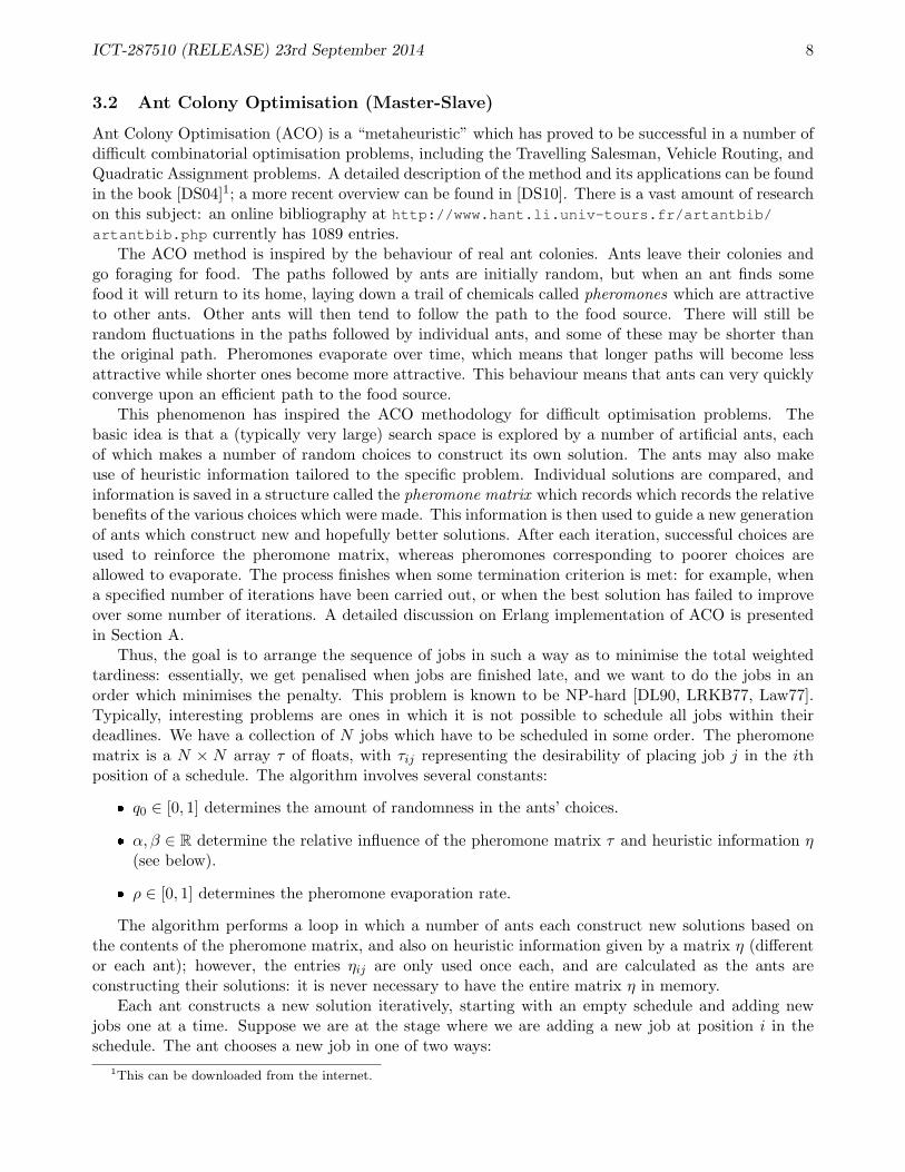
Non-distributed Erlang version. We run the ACO on a single Erlang node (Figure 7). Thepheromone matrix is represented as an ETS table which stores each row of the matrix as an N -tuple ofreal numbers. This is accessible to all processes running in the Erlang VM. The program takes three
ICT-287510 (RELEASE) 23rd September 2014 10
Figure 7: ACO in Non-distributed Erlang
arguments. The first argument is the name of a file containing input data: an integer N and 3 sets ofN integers, representing the processing times, the weights, and the deadlines for each job. The secondargument is the number M of ants which should be used, and the third argument is the number K ofiterations of the main “loop” of the program, i.e. the number of generations of ants.
After reading its inputs, the program creates and initialises the table representing the pheromonematrix, then spawns M ant processes. The program then enters a loop in which the following happens:
� The ants construct new solutions in parallel.
� When an ant finishes creating its solution, it sends a message containing the solution and its totaltardiness to a master process.
� The master compares the incoming messages against the current best solution.
� After all M results have been received, the master uses the new best solution to update thepheromone matrix.
� A new iteration is then started: again, each ant constructs a new solution.
� After K iterations, the program terminates and outputs its best solution.
The execution time of the program is linear in the number of iterations K and quadratic in size ofthe matrix N due to data allocation and also due to the fact that since the entire N ×N matrix τ hasto be traversed by each ant and later rewritten in the global update stage. It is more difficult to seehow the execution time is influenced by the number of ants M , although it appears to vary linearly.The details can be found in Section A.3.2.
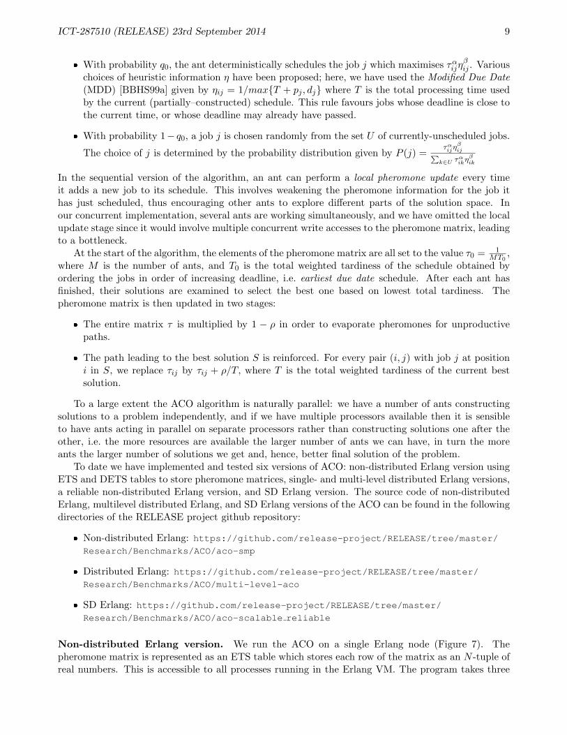
Non2D. A number of Erlang VMs are started on different machines in a network, and each of theseruns a single colony (Figure 8). There is a single master node which starts the colonies and distributesinformation (like the input data and parameter settings) to them; each colony runs a specified numberof ants for a specified number of generations, and then reports its best solution back to the master. Themaster chooses the best solution from among the colonies and then broadcasts it to all of the colonies,which use it to update their pheromone matrices and then start another round of iterations. Sharingonly the best solution allows colonies to influence each other while retaining some individuality. Thisreduces the amount of data transfer significantly: instead of having to transmit N2 floats, we only haveto transfer N integers. The entire process is repeated some number of times, after which the mastershuts down the colonies and reports the best result. For details see Section A.4.
Summary. We introduce two types of nodes: a master node and slave nodes. The master nodecontains a master process, and the slave nodes contain the colonies. Each node has its own pheromone
ICT-287510 (RELEASE) 23rd September 2014 11
Figure 8: ACO in Distributed Erlang
matrix. The master process collects pheromone results, picks the best one, and distributes it back tothe colonies. The colonies are spawned by the master process in the beginning – one colony per slavenode, and during the rest of the computation no other new processes are spawned to remote nodes.
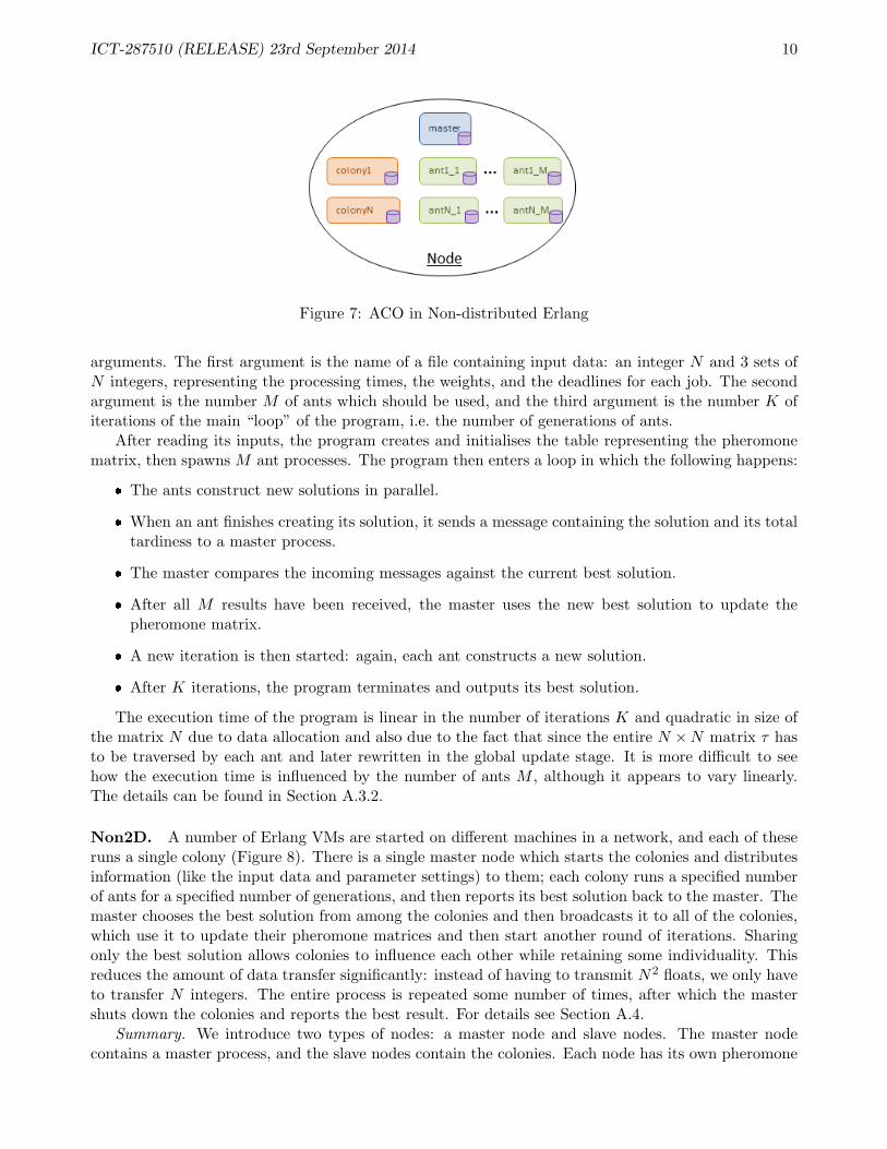
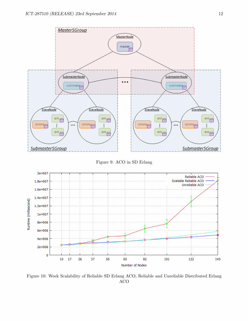
D2SD. In the SD Erlang implementation of ACO we introduce yet one more type of nodes – submasternodes (Figure 9). We partition the set of slave nodes into groups and add a submaster node to everypartition – these are submaster s groups. The master node and submaster nodes form a master s group.The colonies on slave nodes run computation and periodically send results to their submaster nodes.The submaster nodes collect results from their slave nodes, pick the best solution, and distribute it backto the colonies. The submaster nodes also periodically send results to the master node. The masternode collects results, picks the best solution, and distributes it back to the submaster nodes, after thatthe submaster nodes forward the result to their slave nodes.
Summary. To refactor a distributed Erlang ACO into an SD Erlang one we do the following: (1)partition slave nodes, add submaster nodes, and group nodes into submaster and master s groups, (2)share the master process functionality with submaster processes.
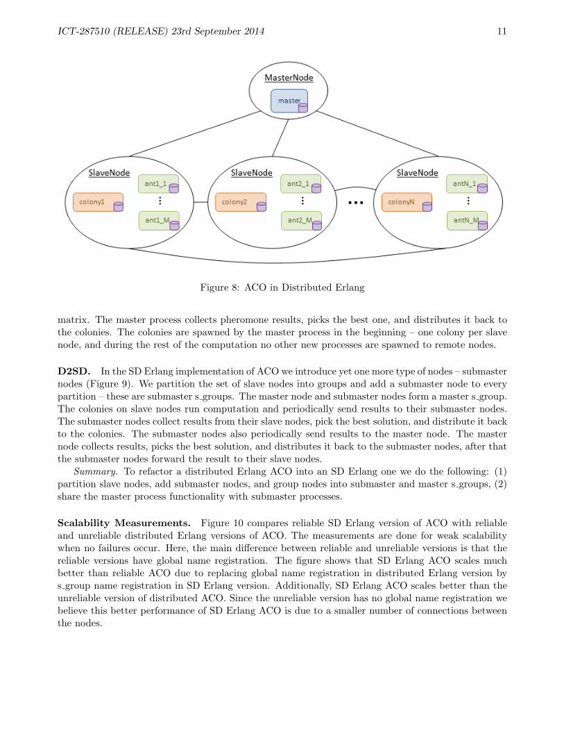
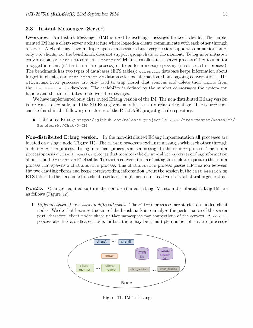
Scalability Measurements. Figure 10 compares reliable SD Erlang version of ACO with reliableand unreliable distributed Erlang versions of ACO. The measurements are done for weak scalabilitywhen no failures occur. Here, the main difference between reliable and unreliable versions is that thereliable versions have global name registration. The figure shows that SD Erlang ACO scales muchbetter than reliable ACO due to replacing global name registration in distributed Erlang version bys group name registration in SD Erlang version. Additionally, SD Erlang ACO scales better than theunreliable version of distributed ACO. Since the unreliable version has no global name registration webelieve this better performance of SD Erlang ACO is due to a smaller number of connections betweenthe nodes.
ICT-287510 (RELEASE) 23rd September 2014 12
Figure 9: ACO in SD Erlang
Figure 10: Week Scalability of Reliable SD Erlang ACO, Reliable and Unreliable Distributed ErlangACO
ICT-287510 (RELEASE) 23rd September 2014 13
3.3 Instant Messenger (Server)
Overview. An Instant Messenger (IM) is used to exchange messages between clients. The imple-mented IM has a client-server architecture where logged-in clients communicate with each other througha server. A client may have multiple open chat sessions but every session supports communication ofonly two clients, i.e. the benchmark does not support group chats at the moment. To log-in or initiate aconversation a client first contacts a router which in turn allocates a server process either to monitora logged-in client (client monitor process) or to perform message passing (chat session process).The benchmark has two types of databases (ETS tables): client db database keeps information aboutlogged-in clients, and chat session db database keeps information about ongoing conversations. Theclient monitor processes are only used to trap closed chat sessions and delete their entries fromthe chat session db database. The scalability is defined by the number of messages the system canhandle and the time it takes to deliver the messages.
We have implemented only distributed Erlang version of the IM. The non-distributed Erlang versionis for consistency only, and the SD Erlang version is in the early refactoring stage. The source codecan be found in the following directories of the RELEASE project github repository:
� Distributed Erlang: https://github.com/release-project/RELEASE/tree/master/Research/Benchmarks/Chat/D-IM
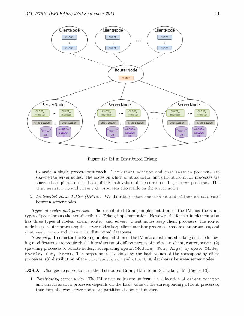
Non-distributed Erlang version. In the non-distributed Erlang implementation all processes arelocated on a single node (Figure 11). The client processes exchange messages with each other througha chat session process. To log-in a client process sends a message to the router process. The routerprocess spawns a client monitor process that monitors the client and keeps corresponding informationabout it in the client db ETS table. To start a conversation a client again sends a request to the routerprocess that spawns a chat session process. The chat session process passes information betweenthe two chatting clients and keeps corresponding information about the session in the chat session db
ETS table. In the benchmark no client interface is implemented instead we use a set of traffic generators.
Non2D. Changes required to turn the non-distributed Erlang IM into a distributed Erlang IM areas follows (Figure 12).
1. Different types of processes on different nodes. The client processes are started on hidden clientnodes. We do that because the aim of the benchmark is to analyse the performance of the serverpart; therefore, client nodes share neither namespace nor connections of the servers. A router
process also has a dedicated node. In fact there may be a multiple number of router processes
Figure 11: IM in Erlang
ICT-287510 (RELEASE) 23rd September 2014 14
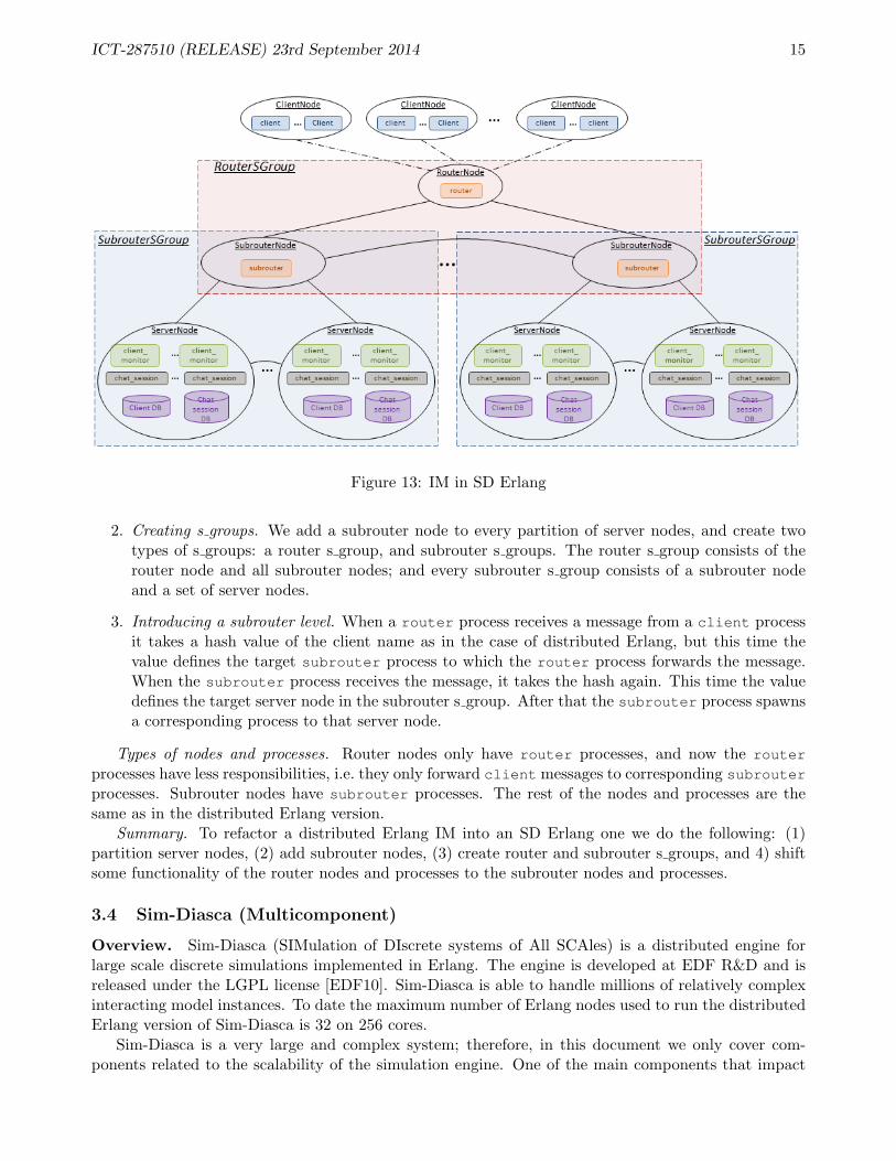
Figure 12: IM in Distributed Erlang
to avoid a single process bottleneck. The client monitor and chat session processes arespawned to server nodes. The nodes on which chat session and client monitor processes arespawned are picked on the basis of the hash values of the corresponding client processes. Thechat session db and client db processes also reside on the server nodes.
2. Distributed Hash Tables (DHTs). We distribute chat session db and client db databasesbetween server nodes.
Types of nodes and processes. The distributed Erlang implementation of the IM has the sametypes of processes as the non-distributed Erlang implementation. However, the former implementationhas three types of nodes: client, router, and server. Client nodes keep client processes; the routernode keeps router processes; the server nodes keep client monitor processes, chat session processes, andchat session db and client db distributed databases.
Summary. To refactor the Erlang implementation of the IM into a distributed Erlang one the follow-ing modifications are required: (1) introduction of different types of nodes, i.e. client, router, server; (2)spawning processes to remote nodes, i.e. replacing spawn(Module, Fun, Args) by spawn(Node,Module, Fun, Args). The target node is defined by the hash values of the corresponding clientprocesses; (3) distribution of the chat session db and client db databases between server nodes.
D2SD. Changes required to turn the distributed Erlang IM into an SD Erlang IM (Figure 13).
1. Partitioning server nodes. The IM server nodes are uniform, i.e. allocation of client monitor
and chat session processes depends on the hash value of the corresponding client processes,therefore, the way server nodes are partitioned does not matter.
ICT-287510 (RELEASE) 23rd September 2014 15
Figure 13: IM in SD Erlang
2. Creating s groups. We add a subrouter node to every partition of server nodes, and create twotypes of s groups: a router s group, and subrouter s groups. The router s group consists of therouter node and all subrouter nodes; and every subrouter s group consists of a subrouter nodeand a set of server nodes.
3. Introducing a subrouter level. When a router process receives a message from a client processit takes a hash value of the client name as in the case of distributed Erlang, but this time thevalue defines the target subrouter process to which the router process forwards the message.When the subrouter process receives the message, it takes the hash again. This time the valuedefines the target server node in the subrouter s group. After that the subrouter process spawnsa corresponding process to that server node.
Types of nodes and processes. Router nodes only have router processes, and now the router
processes have less responsibilities, i.e. they only forward client messages to corresponding subrouter
processes. Subrouter nodes have subrouter processes. The rest of the nodes and processes are thesame as in the distributed Erlang version.
Summary. To refactor a distributed Erlang IM into an SD Erlang one we do the following: (1)partition server nodes, (2) add subrouter nodes, (3) create router and subrouter s groups, and 4) shiftsome functionality of the router nodes and processes to the subrouter nodes and processes.
3.4 Sim-Diasca (Multicomponent)
Overview. Sim-Diasca (SIMulation of DIscrete systems of All SCAles) is a distributed engine forlarge scale discrete simulations implemented in Erlang. The engine is developed at EDF R&D and isreleased under the LGPL license [EDF10]. Sim-Diasca is able to handle millions of relatively complexinteracting model instances. To date the maximum number of Erlang nodes used to run the distributedErlang version of Sim-Diasca is 32 on 256 cores.
Sim-Diasca is a very large and complex system; therefore, in this document we only cover com-ponents related to the scalability of the simulation engine. One of the main components that impact
ICT-287510 (RELEASE) 23rd September 2014 16
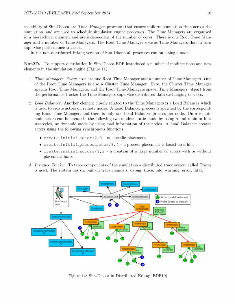
scalability of Sim-Diasca are Time Manager processes that ensure uniform simulation time across thesimulation, and are used to schedule simulation engine processes. The Time Managers are organisedin a hierarchical manner, and are independent of the number of cores. There is one Root Time Man-ager and a number of Time Managers. The Root Time Manager spawns Time Managers that in turnsupervise performance trackers.
In the non-distributed Erlang version of Sim-Diasca all processes run on a single node.
Non2D. To support distribution in Sim-Diasca EDF introduced a number of modifications and newelements in the simulation engine (Figure 14).
1. Time Managers. Every host has one Root Time Manager and a number of Time Managers. Oneof the Root Time Managers is also a Cluster Time Manager. Here, the Cluster Time Managerspawns Root Time Managers, and the Root Time Managers spawn Time Managers. Apart fromthe performance tracker the Time Managers supervise distributed data-exchanging services.
2. Load Balancer. Another element closely related to the Time Managers is a Load Balancer whichis used to create actors on remote nodes. A Load Balancer process is spawned by the correspond-ing Root Time Manager, and there is only one Load Balancer process per node. On a remotenode actors can be create in the following two modes: static mode by using round-robin or hintstrategies, or dynamic mode by using load information of the nodes. A Load Balancer createsactors using the following synchronous functions:
� create initial actor/2,3 – no specific placement
� create initial placed actor/3,4 – a process placement is based on a hint
� create initial actors/1,2 – a creation of a large number of actors with or withoutplacement hints
3. Instance Tracker. To trace components of the simulation a distributed trace system called Tracesis used. The system has six built-in trace channels: debug, trace, info, warning, error, fatal.
Figure 14: Sim-Diasca in Distributed Erlang [EDF10]
ICT-287510 (RELEASE) 23rd September 2014 17
4. Data Exchanger is a distributed simulation service that is used to share data between actorslocally. It is distributed in terms of any actor from a particular node can access data from itsData Exchanger with a negligibly low latency.
Types of nodes and processes. There are two types of nodes: a user node and computing nodes.The user node initiates the simulation and then collects statistics and results of the simulation. Thecomputing nodes perform the actual simulation. Apart from the user host that may contain twonodes – the user node and a computing node – every host contains only one node (a computingnode). All nodes are interconnected and are known in advance, i.e. the participating hosts are listed insim-diasca-host-candidates.txt.
Summary. In the distributed Erlang version two types of nodes were introduced: a client nodeand computing nodes. To synchronise simulation time across nodes an additional level of hierarchy forTime Managers was introduced. An introducing of load management and hint mechanisms enabledto distribute load between nodes. To spawn a process the target node is defined either by a hint (toplace frequently communicating processes close to each other) or by load balancing (the processes arespawned to the least loaded nodes).
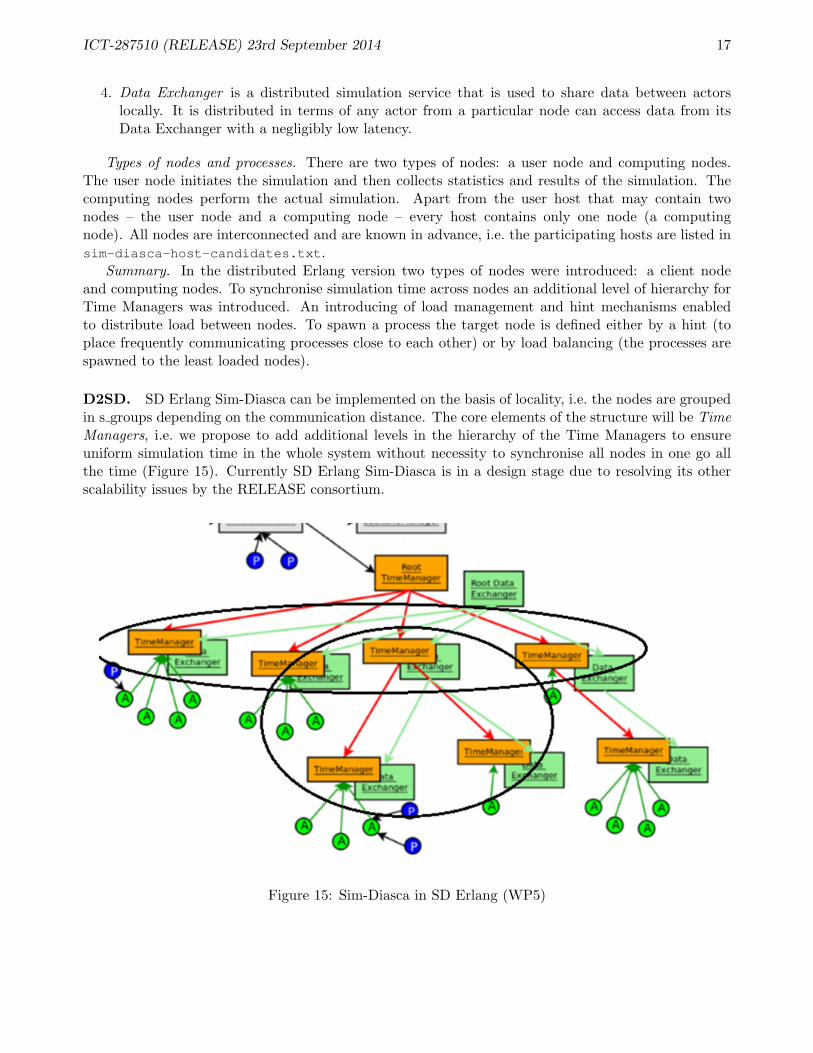
D2SD. SD Erlang Sim-Diasca can be implemented on the basis of locality, i.e. the nodes are groupedin s groups depending on the communication distance. The core elements of the structure will be TimeManagers, i.e. we propose to add additional levels in the hierarchy of the Time Managers to ensureuniform simulation time in the whole system without necessity to synchronise all nodes in one go allthe time (Figure 15). Currently SD Erlang Sim-Diasca is in a design stage due to resolving its otherscalability issues by the RELEASE consortium.
Figure 15: Sim-Diasca in SD Erlang (WP5)
ICT-287510 (RELEASE) 23rd September 2014 18
3.5 Summary
The refactoring of non-distributed Erlang applications into distributed Erlang ones, and then dis-tributed Erlang applications into SD Erlang ones is very much application specific. However, we canidentify some common patters.
Refactoring a non-distributed Erlang application into a distributed Erlang one.
1. Spawning processes to remote nodes, i.e. replacing spawn(Module, Fun, Args) by spawn(Node,Module, Fun, Args) and defining the target nodes.
2. Introducing distributed databases, e.g. the DHT in SD Orbit.
3. Tuning the performance, i.e. deciding on the right number of different types of nodes and processes.
Refactoring a distributed Erlang application into an SD Erlang one:
1. Grouping nodes in s groups. Depending on the application we may need the following: (a) definethe structure of s groups (e.g. hierarchical, ring, star), (b) decide which nodes it is better togroup, (c) add gateway processes and a corresponding functionality to enable remote nodes tocommunicate with each other without establishing a direct connection, (d) introduce submasternodes and processes and shift on them some functionality from the master nodes and processesto offload the later.
2. Tuning the performance by determining the size of s groups and the number of gateway processes.
We further discuss SD Erlang scalability principles and application methodology in Section 4.1.3.
4 Distributed Erlang Scalability Principles & Application Method-ology
In this section we focus on distributed Erlang scalability issues that is we do not cover single nodescalability issues. The later can be found elsewhere, e.g. deliverables of WP2 and [CV14, Arm13, CT09].We start with all-to-all connections (Section 4.1), then discuss global namespace (Section 4.2), and finishwith a discussion on single process bottleneck issues (Section 4.3).
4.1 Replacing All-to-all Connections
4.1.1 Issues with All-to-all Connections.
In many distributed Erlang systems nodes are normal and the flag of transitive connectivity is set; so, allnodes in the system are interconnected. Thus the total number of connections is n(n− 1)/2, and everynode supports (n − 1) connections. Every connection requires a separate TCP/IP port. When nodesare connected they monitor each other by sending heartbeat messages. In small systems maintaining,a fully connected network is not an issue; however, when either traffic or the number of nodes grows afully connected network requires significant resources and becomes a burden to maintain. For example,in a heavily loaded game server a fully connected network of 16 nodes becomes an issue, less loadedapplications may display difficulty in maintaining a fully connected network at approximately 70-200nodes [GCTM13].
ICT-287510 (RELEASE) 23rd September 2014 19
4.1.2 Ad Hoc Approaches
There are a number of approaches that Erlang developers use to overcome the issue of a fully connectednetwork in distributed Erlang.
One game company disables transitive connectivity flag and manually connects normal nodes ac-cording to some topology. In this case, the nodes have normal node properties but do not share connec-tions, and the whole application is built around preventing nodes from establishing new connections.In March 2014 the company was dealing with up to 16 Erlang nodes.
Another game company Spil Games [Spi14] uses hidden nodes and a predefined configuration. Theconfiguration contains a set of nodes the current node is allowed to connect to. The mechanism issuitable for systems with well defined types of nodes similar to a web server where particular types ofnodes are responsible for particular parts of a web-page. Additionally, nodes do not require a commonnamespace, i.e. if needed this mechanism should be implemented separately. The mechanism reportedlyscales up to a thousand Erlang nodes.
Another approach is using OTP global groups by partitioning a set of nodes into global groups.Each group has its own namespace. Nodes within the global group have transitive connections, andnon-transitive connections with nodes outside of the global group. The drawback is that the approachis limited to the cases when the network can be partitioned.
4.1.3 RELEASE Approach: s groups
In the RELEASE project we have introduced s groups which are similar to global groups in that eachs group has its own namespace, and transitive connections are only with nodes of the same s group. Thedifference with global groups is in that a node can belong to an unlimited number of s groups which en-ables to form different types of topologies. To create a new s group the s group:new s group(SGroupName,
[Node]) function is used. We can also add nodes to an s group using s group:add nodes(SGroupName,
[Node]) function, remove nodes from an s group using s group:remove nodes(SGroupName, [Node])
function, and delete an s group using s group:delete s group(SGroupName) function. Details of SDErlang implementation and its functions are covered in the following RELEASE project deliverables:D3.2: Scalable SD Erlang Computation Model [REL13a] and D3.3: Scalable SD Erlang ReliabilityModel [REL13b].
When s groups are arranged in a hierarchical manner one can find similarities between Erlang nodesthat belong to a number of s groups (let us call them gateway nodes) and super-peers, i.e. nodes thatact simultaneously as a server and a peer [BYGM03]. However, in SD Erlang whether a gateway nodehas a super-peer functionality depends on the application and is not imposed by s groups.
The reason we have introduced s groups was to reduce the number of connections a node maintainsbut at the same time provide nodes an opportunity to keep distributed Erlang connections, i.e. whena node joins an s group it is automatically connected to all nodes in that s group. Another aim was toreduce the common namespace which in distributed Erlang and in SD Erlang is closely connected totransitive connectivity. We discuss impact of shared namespace in Section 4.2.
In the exemplars we discuss in Section 3 the sets of nodes are arranged in a hierarchical mannerin SD Erlang. A natural question would be “Why not introduce hierarchical s groups with a built-inrouting instead of overlapping s groups where routing should be implemented individually dependingon an application”. The reason is that by introducing SD Erlang we aimed to provide a tool that adeveloper can use to reduce the number of connections but keep Erlang distribution properties andfunctionality between some groups of nodes, rather than introducing a scheme that developers wouldhave to fit their application in.
How to structure nodes to scale? To scale a set of Erlang nodes the nodes can be structured, forexample, in a hierarchical manner. In this case if we have a master node it should be at the root of the
ICT-287510 (RELEASE) 23rd September 2014 20
system, and the worker nodes are leaves. S groups can also be arranged in, for example, a ring or starmanner.
Which nodes to group? To identify the most suitable nodes to group in s groups Percept2 [REL14c]and devo [REL14b] tools that WP5 is developing can be used. Percept2 can show how the communi-cation between nodes works, and devo will be able to show how nodes have affinity with each other.The discussion on devo tool and examples on how to use it is planed to be discussed in the upcomingdeliverable D5.4: Interactive SD Erlang Debugger.
How to determine the size of s groups? The size of an s group depends on the intensity of theinter- and intra-s group communication, and global operations. The larger these parameters the smallerthe number of nodes in the s group. To analyse intra- and inter-s group communications the devo toolcan be used. Further discussion on tools and examples on automating generic parts of the refactoringprocess is provided in deliverable D5.3: Systematic Testing and Debugging Tools [REL14a].
In the exemplars from Section 3 we observed patterns in grouping nodes, i.e. partitioning, hierar-chical grouping, and hierarchical grouping with redundancy. To automate and simplify the mechanismof grouping nodes we propose s group:grouping/1 function that takes a list of nodes together withsome additional parameters, creates s groups, and returns a result. Below we discuss the details of eachtype of grouping.
4.1.4 Functions to Group Nodes
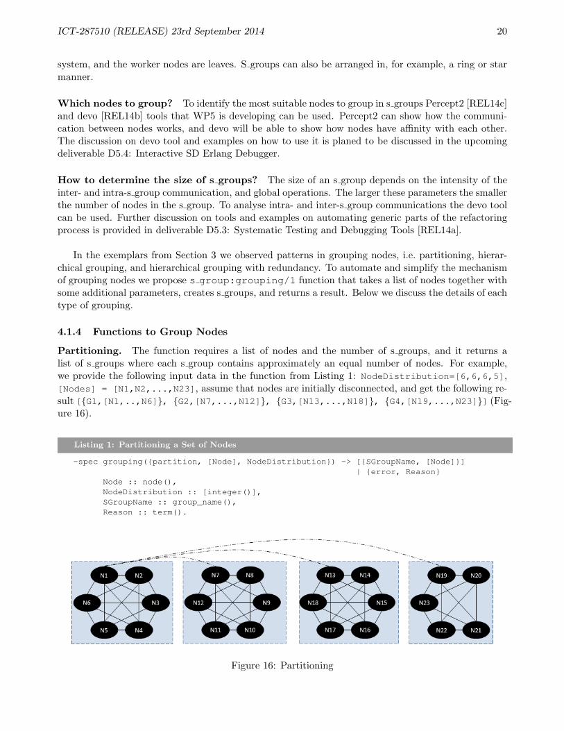
Partitioning. The function requires a list of nodes and the number of s groups, and it returns alist of s groups where each s group contains approximately an equal number of nodes. For example,we provide the following input data in the function from Listing 1: NodeDistribution=[6,6,6,5],[Nodes] = [N1,N2,...,N23], assume that nodes are initially disconnected, and get the following re-sult [{G1,[N1,..,N6]}, {G2,[N7,...,N12]}, {G3,[N13,...,N18]}, {G4,[N19,...,N23]}] (Fig-ure 16).
Listing 1: Partitioning a Set of Nodes
-spec grouping({partition, [Node], NodeDistribution}) -> [{SGroupName, [Node]}]| {error, Reason}
Node :: node(),NodeDistribution :: [integer()],SGroupName :: group_name(),Reason :: term().
Figure 16: Partitioning

ICT-287510 (RELEASE) 23rd September 2014 21
Figure 17: Hierarchical: no root level + 2 levels
Figure 18: Hierarchical: a root level of one node + 2 levels
Hierarchical grouping. The function requires a list of nodes and the node distribution on each level(Listing 2). Depending on the values of NodeDistribution parameter the hierarchical grouping mayhave a number or none of root nodes, and a different number of levels.
Listing 2: Hierarchical Structure with a Single Root Node
-spec grouping({hierarchical, [Nodes], NodeDistribution}) -> [{SGroupName, [Node]}]| {error, Reason}
Node :: node(),NodeDistribution :: [term()],SGroupName :: group_name(),Reason :: term().
For example, we have 23 disconnected nodes and we want to group them in a number of ways, e.g.
� No root level + 2 levels (Figure 17). In this case NodeDistribution=[0,[4],[4,7,3,5]].
ICT-287510 (RELEASE) 23rd September 2014 22
� 3 levels with a root node (Figure 18). In this case NodeDistribution=[1,[4],[5,5,4,4]].
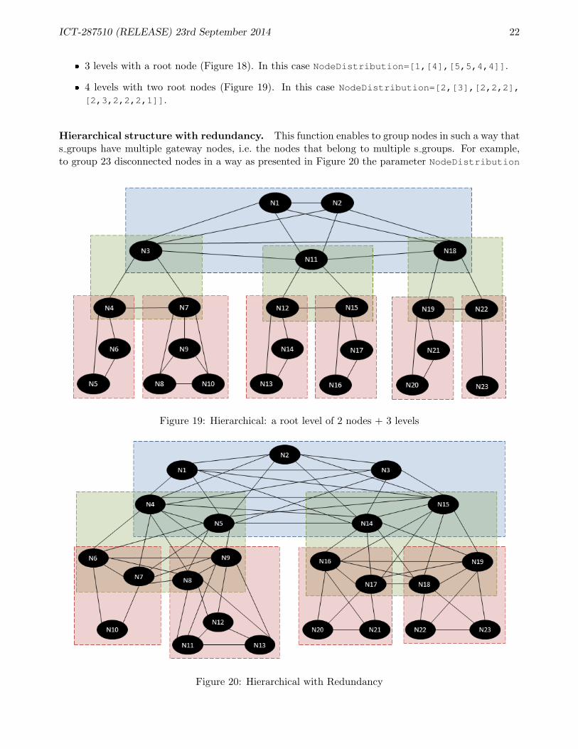
� 4 levels with two root nodes (Figure 19). In this case NodeDistribution=[2,[3],[2,2,2],
[2,3,2,2,2,1]].
Hierarchical structure with redundancy. This function enables to group nodes in such a way thats groups have multiple gateway nodes, i.e. the nodes that belong to multiple s groups. For example,to group 23 disconnected nodes in a way as presented in Figure 20 the parameter NodeDistribution
Figure 19: Hierarchical: a root level of 2 nodes + 3 levels
Figure 20: Hierarchical with Redundancy
ICT-287510 (RELEASE) 23rd September 2014 23
from Listing 3 should be as follows NodeDistribution=[3,[4],[2,4,2,4],[2,1,2,3,2,2,2,2]]].
Listing 3: Hierarchical Structure with Redundancy
-spec grouping({hierarchical_redundancy, [Nodes], NodeDistribution}) ->[{SGroupName, [Node]}] | {error, Reason}
Node :: node(),NodeDistribution :: [term()],SGroupName :: group_name(),Reason :: term().
4.2 Replacing Global Namespace
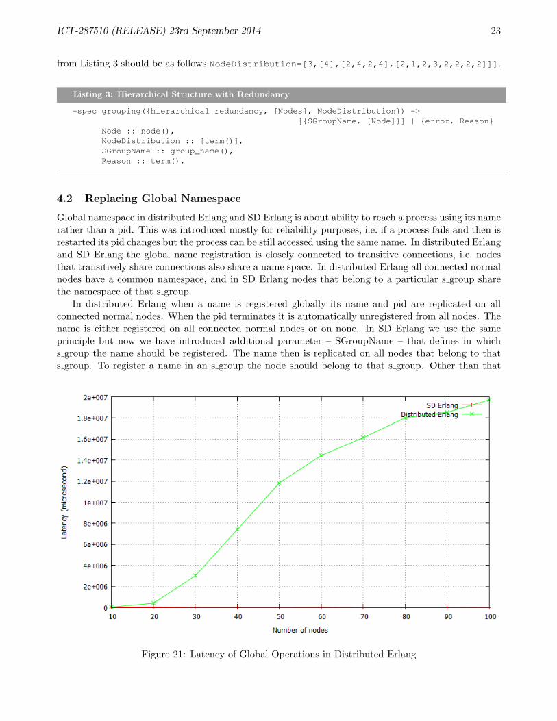
Global namespace in distributed Erlang and SD Erlang is about ability to reach a process using its namerather than a pid. This was introduced mostly for reliability purposes, i.e. if a process fails and then isrestarted its pid changes but the process can be still accessed using the same name. In distributed Erlangand SD Erlang the global name registration is closely connected to transitive connections, i.e. nodesthat transitively share connections also share a name space. In distributed Erlang all connected normalnodes have a common namespace, and in SD Erlang nodes that belong to a particular s group sharethe namespace of that s group.
In distributed Erlang when a name is registered globally its name and pid are replicated on allconnected normal nodes. When the pid terminates it is automatically unregistered from all nodes. Thename is either registered on all connected normal nodes or on none. In SD Erlang we use the sameprinciple but now we have introduced additional parameter – SGroupName – that defines in whichs group the name should be registered. The name then is replicated on all nodes that belong to thats group. To register a name in an s group the node should belong to that s group. Other than that
Figure 21: Latency of Global Operations in Distributed Erlang
ICT-287510 (RELEASE) 23rd September 2014 24
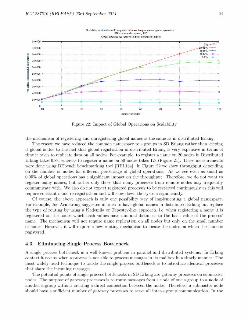
Figure 22: Impact of Global Operations on Scalability
the mechanism of registering and unregistering global names is the same as in distributed Erlang.The reason we have reduced the common namespace to s groups in SD Erlang rather than keeping
it global is due to the fact that global registration in distributed Erlang is very expensive in terms oftime it takes to replicate data on all nodes. For example, to register a name on 20 nodes in DistributedErlang takes 0.8s, whereas to register a name on 50 nodes takes 12s (Figure 21). These measurementswere done using DEbench benchmarking tool [REL13a]. In Figure 22 we show throughput dependingon the number of nodes for different percentage of global operations. As we see even as small as0.05% of global operations has a significant impact on the throughput. Therefore, we do not want toregister many names, but rather only those that many processes from remote nodes may frequentlycommunicate with. We also do not expect registered processes to be restarted continuously as this willrequire constant name re-registration and will slow down the system significantly.
Of course, the above approach is only one possibility way of implementing a global namespace.For example, Joe Armstrong suggested an idea to have global names in distributed Erlang but replacethe type of routing by using a Kademlia or Tapestry-like approach, i.e. when registering a name it isregistered on the nodes which hash values have minimal distances to the hash value of the process’name. The mechanism will not require name replication on all nodes but only on the small numberof nodes. However, it will require a new routing mechanism to locate the nodes on which the name isregistered.
4.3 Eliminating Single Process Bottleneck
A single process bottleneck is a well known problem in parallel and distributed systems. In Erlangcontext it occurs when a process is not able to process messages in its mailbox in a timely manner. Themost widely used technique to tackle the single process bottleneck is to introduce identical processesthat share the incoming messages.
The potential points of single process bottlenecks in SD Erlang are gateway processes on submasternodes. The purpose of gateway processes is to route messages from a node of one s group to a node ofanother s group without creating a direct connection between the nodes. Therefore, a submaster nodeshould have a sufficient number of gateway processes to serve all inter-s group communication. In the
ICT-287510 (RELEASE) 23rd September 2014 25
Orbit example to eliminate a single process bottleneck we have introduced multiple gateway processesper a gateway node. Thus, when a process wants to send a message to a process in another s group,it picks a gateway process randomly. The process of identifying a single process bottleneck in Orbitexample using Percert2 tool [REL14c] developed by the Kent team is demonstrated in [TL13].
5 Reliability Principles
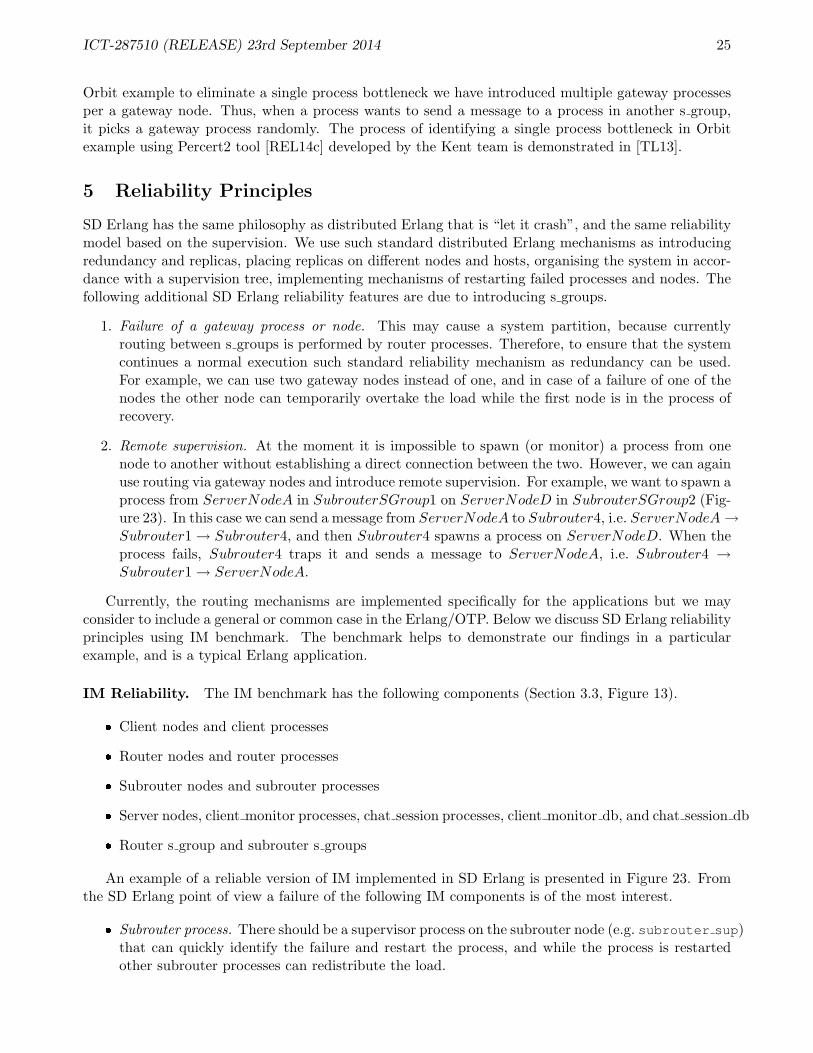
SD Erlang has the same philosophy as distributed Erlang that is “let it crash”, and the same reliabilitymodel based on the supervision. We use such standard distributed Erlang mechanisms as introducingredundancy and replicas, placing replicas on different nodes and hosts, organising the system in accor-dance with a supervision tree, implementing mechanisms of restarting failed processes and nodes. Thefollowing additional SD Erlang reliability features are due to introducing s groups.
1. Failure of a gateway process or node. This may cause a system partition, because currentlyrouting between s groups is performed by router processes. Therefore, to ensure that the systemcontinues a normal execution such standard reliability mechanism as redundancy can be used.For example, we can use two gateway nodes instead of one, and in case of a failure of one of thenodes the other node can temporarily overtake the load while the first node is in the process ofrecovery.
2. Remote supervision. At the moment it is impossible to spawn (or monitor) a process from onenode to another without establishing a direct connection between the two. However, we can againuse routing via gateway nodes and introduce remote supervision. For example, we want to spawn aprocess from ServerNodeA in SubrouterSGroup1 on ServerNodeD in SubrouterSGroup2 (Fig-ure 23). In this case we can send a message from ServerNodeA to Subrouter4, i.e. ServerNodeA→Subrouter1→ Subrouter4, and then Subrouter4 spawns a process on ServerNodeD. When theprocess fails, Subrouter4 traps it and sends a message to ServerNodeA, i.e. Subrouter4 →Subrouter1→ ServerNodeA.
Currently, the routing mechanisms are implemented specifically for the applications but we mayconsider to include a general or common case in the Erlang/OTP. Below we discuss SD Erlang reliabilityprinciples using IM benchmark. The benchmark helps to demonstrate our findings in a particularexample, and is a typical Erlang application.
IM Reliability. The IM benchmark has the following components (Section 3.3, Figure 13).
� Client nodes and client processes
� Router nodes and router processes
� Subrouter nodes and subrouter processes
� Server nodes, client monitor processes, chat session processes, client monitor db, and chat session db
� Router s group and subrouter s groups
An example of a reliable version of IM implemented in SD Erlang is presented in Figure 23. Fromthe SD Erlang point of view a failure of the following IM components is of the most interest.
� Subrouter process. There should be a supervisor process on the subrouter node (e.g. subrouter sup)that can quickly identify the failure and restart the process, and while the process is restartedother subrouter processes can redistribute the load.
ICT-287510 (RELEASE) 23rd September 2014 26
Figure 23: Reliability in SD Erlang IM
� Subrouter node. The subrouter sup process from a remote node should be able to restartthe node together with its subrouter sup process, and then the subrouter sup process willrestart the remaining processes on the node. In the meantime the remaining subrouter nodes candistribute the load. A subrouter node can be monitored from another subrouter node locatedeither in the same or in a remote subrouter s group.
� Subrouter s group. A router sup processes should be able to restart subrouter nodes togetherwith their subrouter sup processes which in turn will restart the remaining components in thes group. The effected clients will need to restart their session which in the meantime will beserved by remaining server nodes. The client monitor db and the chat session db should bereplicated on nodes from remote s group.
6 Performance Portability
One of our aims of the RELEASE project and WP3 in particular is to enable the construction ofdistributed Erlang applications which are not only scalable, but also portable in terms of performance.By this we mean that it should be possible to deploy applications on different systems and achievegood performance with minimal (ideally zero) need for the programmer to tailor the application forthe particular system that the application is running on. For example, some process in a distributedapplication may need to be executed on a machine which has a large amount of RAM, or which
ICT-287510 (RELEASE) 23rd September 2014 27
has a particular library installed, or which can communicate at high speed with the spawning node.Instead of hard-coding the names of suitable nodes into the program, we want to enable applicationsto find suitable nodes automatically at execution time. This would simplify both deployment and codemaintenance. We use the term semi-explicit placement to describe this process. Instead of specifyinga node by its name, a programmer can request (at runtime) a node or list of nodes which conform togiven restrictions.
Our earlier deliverables already include some groundwork for the implementation of performanceportability via semi-explicit placement. In deliverables D3.1: Scalable Reliable SD Erlang Design [REL12,§6] and D3.2: Scalable SD Erlang Computation Model [REL13a, §4], we introduced the choose node/1function which allows a user to select a node to spawn a process on. The specification of choose node/1allows the user to restrict nodes according to s group names, and also according to attributes whichnodes may possess.
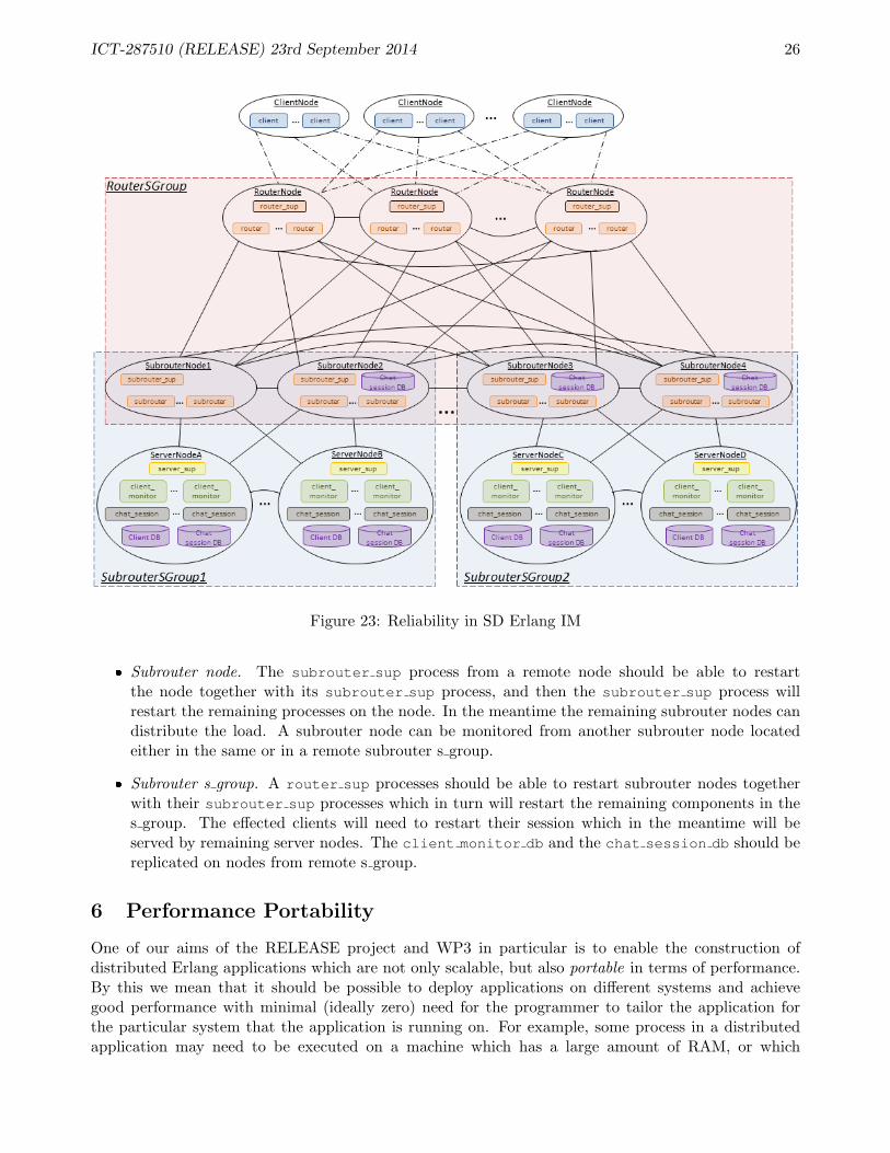
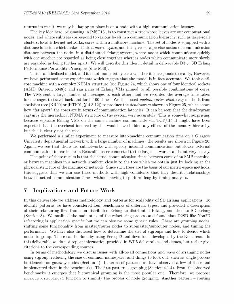
One of the properties we are interested in is communication distance. The idea here is that if twoprocesses are expected to exchange a large number of messages, then they should be placed on nodeswhich can communicate quickly: for example, two nodes running on the same NUMA region of an SMPmachine, or two nodes running on machines which are connected by a high-speed network. Conversely,if a process is expected to perform a lengthy computation with no communication except for when it
(Four sockets like this)
Figure 24: Structure of SMP Machine
ICT-287510 (RELEASE) 23rd September 2014 28
38 39 40 4136 37 46 47 42 43 26 27 12 13 16 1714 15 8 9 6 7 10 11 2 3 4 5 0 1
28 29 30 31 34 35 24 25 20 21 32 33 18 19 22 23 44 45
4000
5000
6000
7000
8000
9000
1000
0
Hei
ght
Figure 25: Communication-time Dendrogram for SMP Machine
amat
eras
u
bwlf2
1
bwlf1
7
bwlf2
6
bwlf2
3
bwlf0
4
bwlf0
7
bwlf3
1
bwlf0
1
bwlf2
0
bwlf1
4
bwlf1
9
bwlf1
8
bwlf2
8
bwlf3
2
bwlf1
1
bwlf2
4
bwlf0
9
bwlf2
2 bwlf1
0
bwlf3
0
bwlf2
5
bwlf2
9 bwlf2
7
bwlf3
3 bwlf0
2
bwlf0
5
bwlf3
4
bwlf0
8
bwlf1
6
bwlf0
3
bwlf0
6
bwlf1
2
bwlf1
3
bwlf1
5 pers
epho
ne
ober
on
cant
or
osiri
s
1200
014
000
1600
018
000
2000
022
000
2400
026
000
Hei
ght
Figure 26: Communication-time Dendrogram for Network
ICT-287510 (RELEASE) 23rd September 2014 29
returns its result, we may be happy to place it on a node with a high communication latency.The key idea here, originating in [MST13], is to construct a tree whose leaves are our computational
nodes, and where subtrees correspond to various levels in a communication hierarchy, such as large-scaleclusters, local Ethernet networks, cores within a multicore machine. The set of nodes is equipped with adistance function which makes it into a metric space, and this gives us a precise notion of communicationdistance between the nodes in a distributed Erlang system, where nodes which communicate quicklywith one another are regarded as being close together whereas nodes which communicate more slowlyare regarded as being further apart. We will describe this idea in detail in deliverable D3.5: SD ErlangPerformance Portability Principles (due M40).
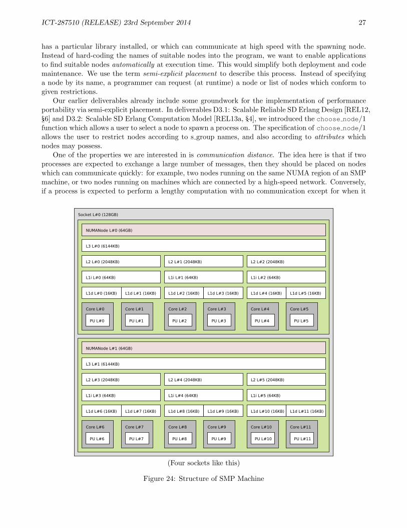
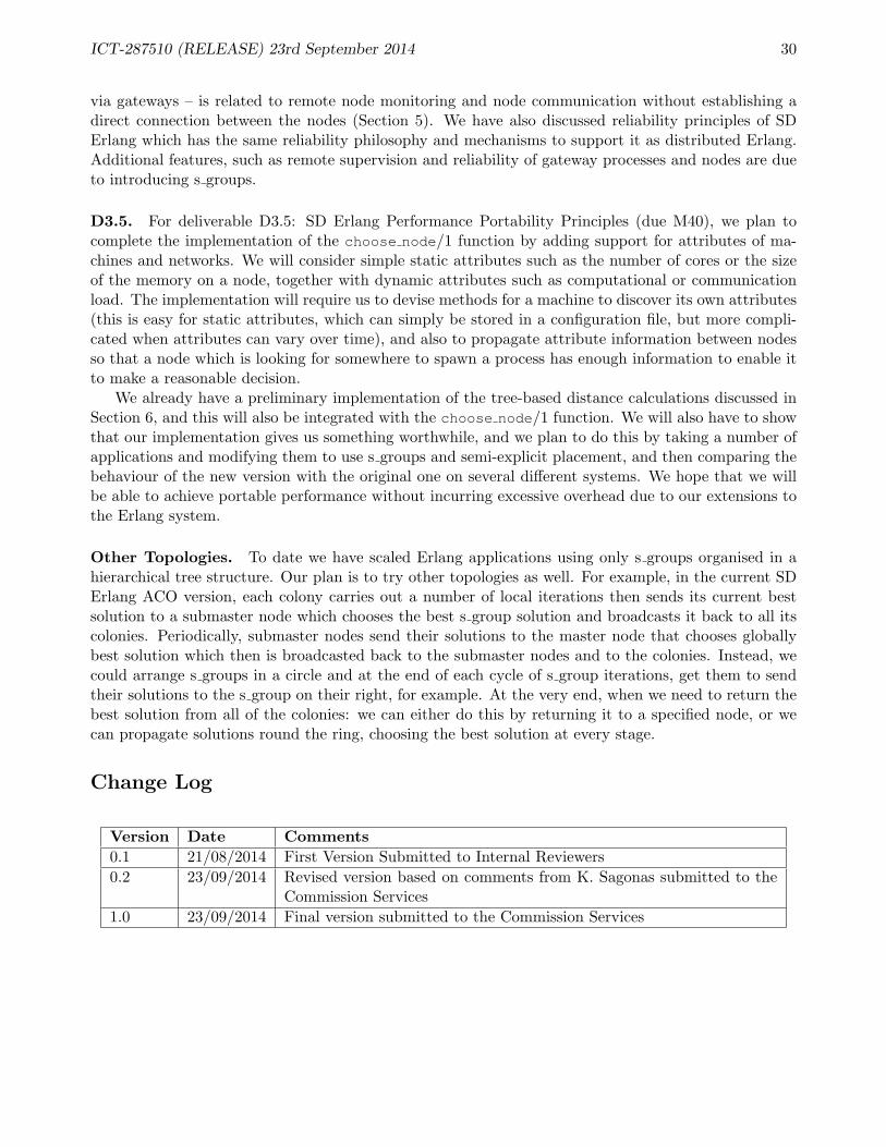
This is an idealised model, and it is not immediately clear whether it corresponds to reality. However,we have performed some experiments which suggest that the model is in fact accurate. We took a 48-core machine with a complex NUMA structure (see Figure 24, which shows one of four identical sockets(AMD Opteron 6348)) and ran pairs of Erlang VMs pinned to all possible combinations of cores.The VMs sent a large number of messages to each other, and we recorded the average time takenfor messages to travel back and forth 100 times. We then used agglomerative clustering methods fromstatistics (see [KR90] or [HTF01, §14.3.12]) to produce the dendrogram shown in Figure 25, which showshow “far apart” the cores are in terms of communication latencies. It can be seen that the dendrogramcaptures the hierarchical NUMA structure of the system very accurately. This is somewhat surprising,because separate Erlang VMs on the same machine communicate via TCP/IP. It might have beenexpected that the overhead incurred by this would have hidden any effects of the memory hierarchy,but this is clearly not the case.
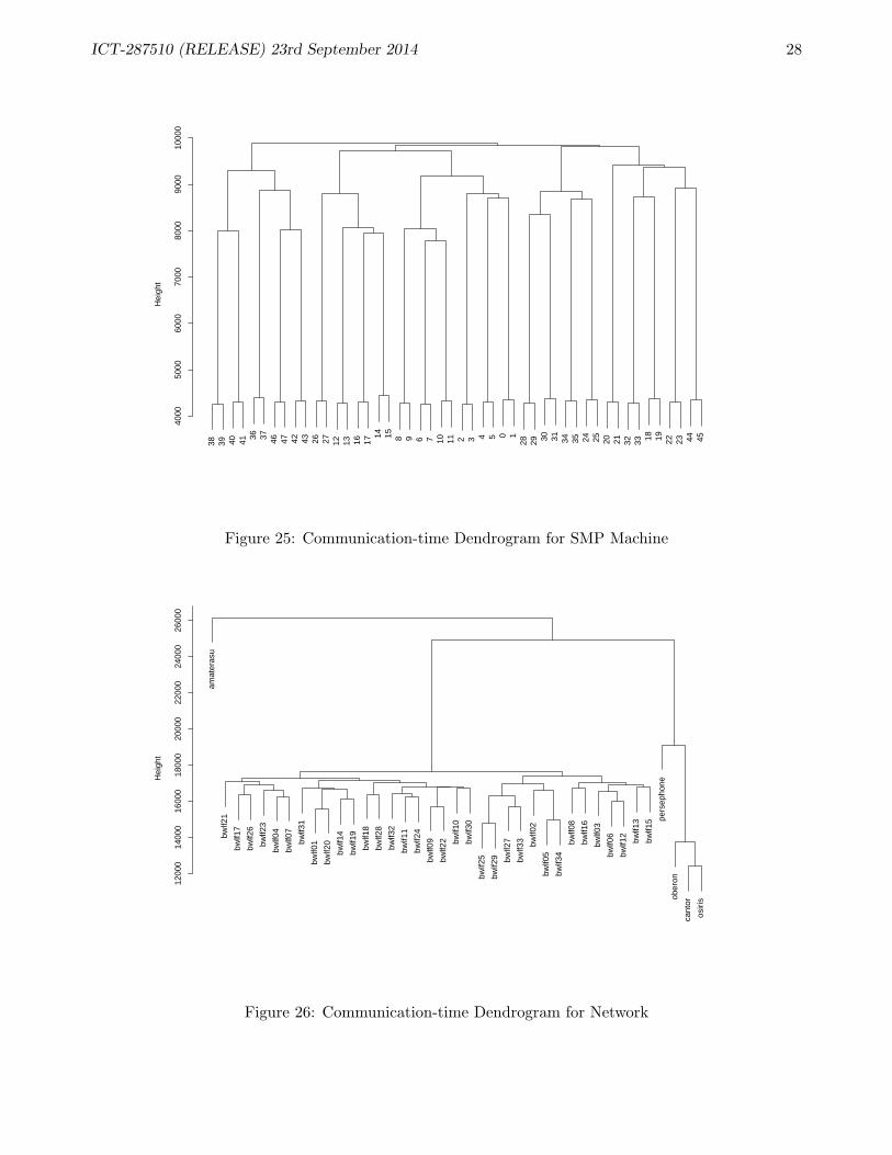
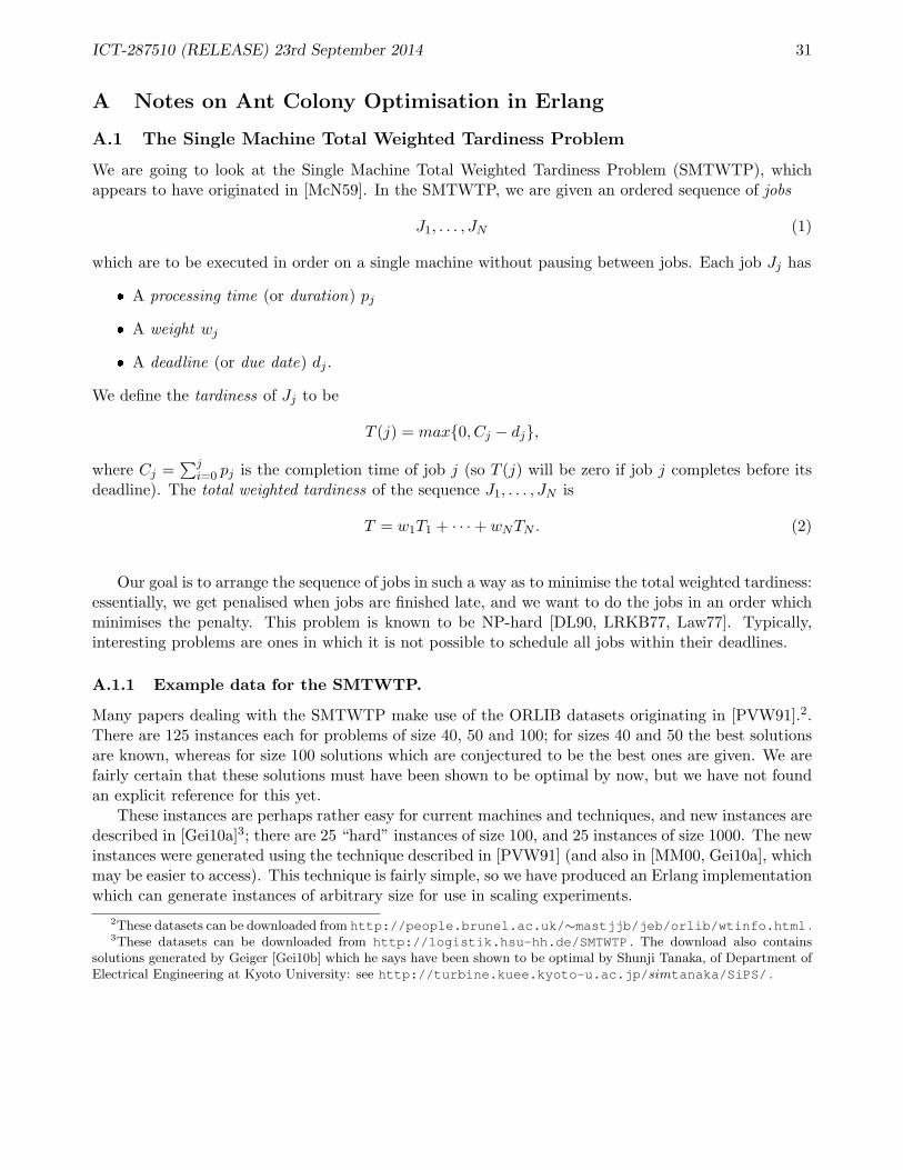
We performed a similar experiment to measure inter-machine communication time on a GlasgowUniversity departmental network with a large number of machines: the results are shown in Figure 26.Again, we see that there are subnetworks with speedy internal communication but slower externalcommunication; in particular, a Beowulf cluster connected to the larger network stands out very clearly.
The point of these results is that the actual communication times between cores of an SMP machine,or between machines in a network, conform closely to the tree which we obtain just by looking at thephysical structure of the machine or network. Since such trees are the basis of our metric-space methods,this suggests that we can use these methods with high confidence that they describe relationshipsbetween actual communication times, without having to perform lengthy timing analyses.
7 Implications and Future Work
In this deliverable we address methodology and patterns for scalability of SD Erlang applications. Toidentify patterns we have considered four benchmarks of different types, and provided a descriptionof their refactoring first from non-distributed Erlang to distributed Erlang, and then to SD Erlang(Section 3). We outlined the main steps of the refactoring process and found that D2SD like Non2Drefactoring is application specific but we can observe some generic rules. These are grouping nodes,shifting some functionality from master/router nodes to submaster/subrouter nodes, and tuning theperformance. We have also discussed how to determine the size of s groups and how to decide whichnodes to group. These can be done by using Persept2 and devo tools developed by the Kent team. Inthis deliverable we do not repeat information provided in WP5 deliverables and demos, but rather givecitations to the corresponding sources.
In terms of methodology we discuss issues with all-to-all connections and ways of arranging nodesusing s group, reducing the size of common namespace, and things to look out, such as single processbottlenecks on gateway nodes (Section 4). In terms of patterns we have observed a few of those andimplemented them in the benchmarks. The first pattern is grouping (Section 4.1.4). From the observedbenchmarks it emerges that hierarchical grouping is the most popular one. Therefore, we proposes group:grouping/1 function to simplify the process of node grouping. Another pattern – routing
ICT-287510 (RELEASE) 23rd September 2014 30
via gateways – is related to remote node monitoring and node communication without establishing adirect connection between the nodes (Section 5). We have also discussed reliability principles of SDErlang which has the same reliability philosophy and mechanisms to support it as distributed Erlang.Additional features, such as remote supervision and reliability of gateway processes and nodes are dueto introducing s groups.
D3.5. For deliverable D3.5: SD Erlang Performance Portability Principles (due M40), we plan tocomplete the implementation of the choose node/1 function by adding support for attributes of ma-chines and networks. We will consider simple static attributes such as the number of cores or the sizeof the memory on a node, together with dynamic attributes such as computational or communicationload. The implementation will require us to devise methods for a machine to discover its own attributes(this is easy for static attributes, which can simply be stored in a configuration file, but more compli-cated when attributes can vary over time), and also to propagate attribute information between nodesso that a node which is looking for somewhere to spawn a process has enough information to enable itto make a reasonable decision.
We already have a preliminary implementation of the tree-based distance calculations discussed inSection 6, and this will also be integrated with the choose node/1 function. We will also have to showthat our implementation gives us something worthwhile, and we plan to do this by taking a number ofapplications and modifying them to use s groups and semi-explicit placement, and then comparing thebehaviour of the new version with the original one on several different systems. We hope that we willbe able to achieve portable performance without incurring excessive overhead due to our extensions tothe Erlang system.
Other Topologies. To date we have scaled Erlang applications using only s groups organised in ahierarchical tree structure. Our plan is to try other topologies as well. For example, in the current SDErlang ACO version, each colony carries out a number of local iterations then sends its current bestsolution to a submaster node which chooses the best s group solution and broadcasts it back to all itscolonies. Periodically, submaster nodes send their solutions to the master node that chooses globallybest solution which then is broadcasted back to the submaster nodes and to the colonies. Instead, wecould arrange s groups in a circle and at the end of each cycle of s group iterations, get them to sendtheir solutions to the s group on their right, for example. At the very end, when we need to return thebest solution from all of the colonies: we can either do this by returning it to a specified node, or wecan propagate solutions round the ring, choosing the best solution at every stage.
Change Log
Version Date Comments0.1 21/08/2014 First Version Submitted to Internal Reviewers0.2 23/09/2014 Revised version based on comments from K. Sagonas submitted to the
Commission Services1.0 23/09/2014 Final version submitted to the Commission Services
ICT-287510 (RELEASE) 23rd September 2014 31
A Notes on Ant Colony Optimisation in Erlang
A.1 The Single Machine Total Weighted Tardiness Problem
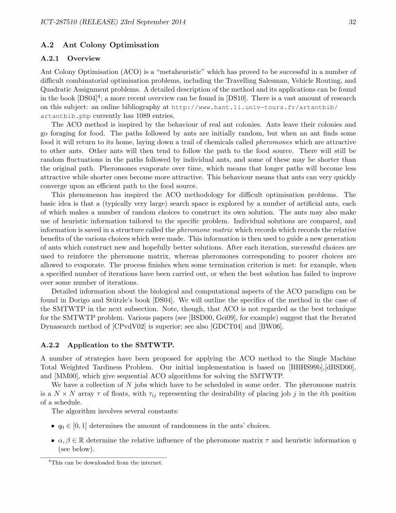
We are going to look at the Single Machine Total Weighted Tardiness Problem (SMTWTP), whichappears to have originated in [McN59]. In the SMTWTP, we are given an ordered sequence of jobs
J1, . . . , JN (1)
which are to be executed in order on a single machine without pausing between jobs. Each job Jj has
� A processing time (or duration) pj
� A weight wj
� A deadline (or due date) dj .
We define the tardiness of Jj to be
T (j) = max{0, Cj − dj},
where Cj =∑j
i=0 pj is the completion time of job j (so T (j) will be zero if job j completes before itsdeadline). The total weighted tardiness of the sequence J1, . . . , JN is
T = w1T1 + · · ·+ wNTN . (2)
Our goal is to arrange the sequence of jobs in such a way as to minimise the total weighted tardiness:essentially, we get penalised when jobs are finished late, and we want to do the jobs in an order whichminimises the penalty. This problem is known to be NP-hard [DL90, LRKB77, Law77]. Typically,interesting problems are ones in which it is not possible to schedule all jobs within their deadlines.
A.1.1 Example data for the SMTWTP.
Many papers dealing with the SMTWTP make use of the ORLIB datasets originating in [PVW91].2.There are 125 instances each for problems of size 40, 50 and 100; for sizes 40 and 50 the best solutionsare known, whereas for size 100 solutions which are conjectured to be the best ones are given. We arefairly certain that these solutions must have been shown to be optimal by now, but we have not foundan explicit reference for this yet.
These instances are perhaps rather easy for current machines and techniques, and new instances aredescribed in [Gei10a]3; there are 25 “hard” instances of size 100, and 25 instances of size 1000. The newinstances were generated using the technique described in [PVW91] (and also in [MM00, Gei10a], whichmay be easier to access). This technique is fairly simple, so we have produced an Erlang implementationwhich can generate instances of arbitrary size for use in scaling experiments.
2These datasets can be downloaded from http://people.brunel.ac.uk/∼mastjjb/jeb/orlib/wtinfo.html .3These datasets can be downloaded from http://logistik.hsu-hh.de/SMTWTP . The download also contains
solutions generated by Geiger [Gei10b] which he says have been shown to be optimal by Shunji Tanaka, of Department ofElectrical Engineering at Kyoto University: see http://turbine.kuee.kyoto-u.ac.jp/simtanaka/SiPS/ .
ICT-287510 (RELEASE) 23rd September 2014 32
A.2 Ant Colony Optimisation
A.2.1 Overview
Ant Colony Optimisation (ACO) is a “metaheuristic” which has proved to be successful in a number ofdifficult combinatorial optimisation problems, including the Travelling Salesman, Vehicle Routing, andQuadratic Assignment problems. A detailed description of the method and its applications can be foundin the book [DS04]4; a more recent overview can be found in [DS10]. There is a vast amount of researchon this subject: an online bibliography at http://www.hant.li.univ-tours.fr/artantbib/artantbib.php currently has 1089 entries.
The ACO method is inspired by the behaviour of real ant colonies. Ants leave their colonies andgo foraging for food. The paths followed by ants are initially random, but when an ant finds somefood it will return to its home, laying down a trail of chemicals called pheromones which are attractiveto other ants. Other ants will then tend to follow the path to the food source. There will still berandom fluctuations in the paths followed by individual ants, and some of these may be shorter thanthe original path. Pheromones evaporate over time, which means that longer paths will become lessattractive while shorter ones become more attractive. This behaviour means that ants can very quicklyconverge upon an efficient path to the food source.
This phenomenon has inspired the ACO methodology for difficult optimisation problems. Thebasic idea is that a (typically very large) search space is explored by a number of artificial ants, eachof which makes a number of random choices to construct its own solution. The ants may also makeuse of heuristic information tailored to the specific problem. Individual solutions are compared, andinformation is saved in a structure called the pheromone matrix which records which records the relativebenefits of the various choices which were made. This information is then used to guide a new generationof ants which construct new and hopefully better solutions. After each iteration, successful choices areused to reinforce the pheromone matrix, whereas pheromones corresponding to poorer choices areallowed to evaporate. The process finishes when some termination criterion is met: for example, whena specified number of iterations have been carried out, or when the best solution has failed to improveover some number of iterations.
Detailed information about the biological and computational aspects of the ACO paradigm can befound in Dorigo and Stutzle’s book [DS04]. We will outline the specifics of the method in the case ofthe SMTWTP in the next subsection. Note, though, that ACO is not regarded as the best techniquefor the SMTWTP problem. Various papers (see [BSD00, Gei09], for example) suggest that the IteratedDynasearch method of [CPvdV02] is superior; see also [GDCT04] and [BW06].
A.2.2 Application to the SMTWTP.
A number of strategies have been proposed for applying the ACO method to the Single MachineTotal Weighted Tardiness Problem. Our initial implementation is based on [BBHS99b],[dBSD00],and [MM00], which give sequential ACO algorithms for solving the SMTWTP.
We have a collection of N jobs which have to be scheduled in some order. The pheromone matrixis a N ×N array τ of floats, with τij representing the desirability of placing job j in the ith positionof a schedule.
The algorithm involves several constants:
� q0 ∈ [0, 1] determines the amount of randomness in the ants’ choices.
� α, β ∈ R determine the relative influence of the pheromone matrix τ and heuristic information η(see below).
4This can be downloaded from the internet.
ICT-287510 (RELEASE) 23rd September 2014 33
� ρ ∈ [0, 1] determines the pheromone evaporation rate.
The algorithm performs a loop in which a number of ants each construct new solutions based onthe contents of the pheromone matrix, and also on heuristic information given by a matrix η (differentor each ant); however, the entries ηij are only used once each, and are calculated as the ants areconstructing their solutions: it is never necessary to have the entire matrix η in memory.
Ant behaviour. In detail, each ant constructs a new solution iteratively, starting with an emptyschedule and adding new jobs one at a time. Suppose we are at the stage where we are adding a newjob at position i in the schedule. The ant chooses a new job in one of two ways:
� With probability q0, the ant deterministically schedules the job j which maximises ταijηβij . Various
choices of heuristic information η have been proposed; here, we have used the Modified Due Date(MDD) [BBHS99b] given by
ηij = 1/max{T + pj , dj}
where T is the total processing time used by the current (partially–constructed) schedule. Thisrule favours jobs whose deadline is close to the current time, or whose deadline may already havepassed. Other heuristics commonly used for the SMTWTP are Earliest Due Date (EDD) [Emm69]and Apparent Urgency (AU) [MRV84].
� With probability 1− q0, a job j is chosen randomly from the set U of currently-unscheduled jobs.The choice of j is determined by the probability distribution given by
P (j) =ταijη
βij∑
k∈U ταikη
βik
In the sequential version of the algorithm, an ant can perform a local pheromone update every timeit adds a new job to its schedule. This involves weakening the pheromone information for the job ithas just scheduled, thus encouraging other ants to explore different parts of the solution space. Inour concurrent implementation, several ants are working simultaneously, and we have omitted the localupdate stage since it would involve multiple concurrent write accesses to the pheromone matrix, leadingto a bottleneck.
Global Pheromone Update. At the start of the algorithm, the elements of the pheromone matrixare all set to the value
τ0 =1AT0
,
where M is the number of ants (as usual), and T0 is the total weighted tardiness of the schedule obtainedby ordering the jobs in order of increasing deadline (this is called the Earliest Due Date schedule).
After each ant has finished, their solutions are examined to select the best one (based on lowesttotal tardiness: see Equation A.1). The pheromone matrix is then updated in two stages:
� The entire matrix τ is multiplied by 1 − ρ in order to evaporate pheromones for unproductivepaths.
� The path leading to the best solution S is reinforced. For every pair (i, j) with job j at positioni in S, we replace τij by
τij + ρ/T,
where T is the total weighted tardiness of the current best solution.
ICT-287510 (RELEASE) 23rd September 2014 34
There are many alternative strategies in the literature. For example, all ants may be allowed tocontribute to the pheromone update (possibly weighted according to the quality of their solution);different evaporation strategies may be used; a different reinforcement factor may be used; the entriesof τ may be constrained to lie within some specified maximum and minimum values τmin and τmax.See [DS04] (especially §3.3.3) for details and references.
Parallelisation. To a large extent the ACO algorithm is naturally parallel: we have a number of antsconstructing solutions to a problem independently, and if we have multiple processors available thenis would seem sensible to have ants acting in parallel on separate processors rather than constructingsolutions one after the other. There is some literature on this (see [BKS97, MM98, MM99, RL02, RV09]for example), but perhaps not as much as we would have expected.
Local Search. The basic ACO algorithm generally gets close to a local minimum, but may not findit precisely. The quality of solutions can be improved by performing a local search [CPvW98, dBSD01]just before the global update stage. This involves looking at solutions in some neighbourhood of thecurrent best solution, and moving to the one which improves the solution most. This process is repeateduntil no improvement is found. Various neighbourhood structures have been considered: for example,one may consider schedules which differ by a single interchange of jobs, or one where a single job isremoved and inserted at a different position. Currently, our Erlang implementation includes an optionfor a naive version of local search (techniques such as dynamic programming can be used to improve theefficiency of the search considerably, but we have not yet implemented this). However, we have turnedthis off for the experiments reported below because a considerable amount of computation is requiredand number of iterations is unpredictable: this leads to variations in execution time which obscure theinfluence of the factors which we are really interested in, such as the number of parallel ants.
A.3 Implementation in Erlang (Single Machine)
Our initial implementation runs on a single Erlang node, preferably running on an SMP machine. Werepresent the pheromone matrix as an ETS (or DETS) table which stores each row of the matrix as anN -tuple of real numbers. This is accessible to all processes running in the Erlang VM.
The program takes three arguments. The first argument is the name of a file containing input datafor the SMTWTP problem: this consists of an integer N and 3 sets of N integers, representing theprocessing times, the weights, and the deadlines for each job. The second argument is the number Mof ants which should be used, and the third argument is the number K of iterations of the main “loop”of the program (ie, the number of generations of ants).
After reading its inputs, the program creates and initialises the table representing the pheromonematrix, then spawns M ant processes. The program then enters a loop in which the following happens:
� The ants construct new solutions (as described above) in parallel.
� When an ant finishes creating its solution, it sends a message containing the solution and its totaltardiness to a supervisor process.
� The supervisor compares the incoming messages against the current best solution.
� After all M results have been received, the supervisor uses the new best solution to update thepheromone matrix.
� A new iteration is then started: again, each ant constructs a new solution.
� After K iterations, the program terminates and outputs its best solution.
ICT-287510 (RELEASE) 23rd September 2014 35
A.3.1 Difficulties with Erlang
Two factors make Erlang somewhat unsuitable for implementation of the ACO application.Firstly, a considerable amount of integer and floating-point calculation (including exponentiation)
is performed. There will be some overhead in performing this in the Erlang VM, rather than directlyin C, for example.
More seriously, it is necessary to allocate large amounts of heap space during the calculation. Asmentioned above, it is necessary to calculate some heuristic information, conceptually stored in a matrixη. In fact, we store this information in a list of pairs {j, ηij} where j is the (integer) identifier of ajob, and ηij is the heuristic information indicating the desirability of scheduling job j at the currentposition i in the schedule. We only require information for unscheduled jobs j, but ηij depends on thejobs which have already been scheduled. This means that we must construct a new list every time anant schedules a new job, and thus during the construction of a single schedule each ant must allocateN + (N − 1) + . . .+ 2 = (N2 +N − 2)/2 list cells (each containing a pair {j, ηij}); when we get to thelast job, there is only one choice, so we do not have to allocate a list of length 1). For N = 1000, this is500,499 heap cells which have to be allocated every time an ant constructs a solution (and rememberthat we have multiple ants, each constructing a new solution for every iteration of the main loop ofthe ACO algorithm). In contrast, in C we could use a single array of length N in conjunction withan array saying which jobs are currently unscheduled, and reuse these every time we add a job to theschedule. This would be a massive saving in heap allocation, and it may well be worth using Erlang’snative interface to implement a simple library of mutable arrays with get and set functions.
Addendum. We tried to implement mutable arrays using NIFS, but actually it slowed the wholething down by about another 50%. We are guessing that the problem here is that it is possible to getfloats out of Erlang objects and into C arrays, but there is quite a lot of overhead because you have tounbox an Erlang heap object to get a C double when you write an element of the array, and then whenyou read an element you have to re-box it into an Erlang object again (and this of course requires somenew memory to be allocated in the heap).
One could try to overcome this by storing pointers to boxed objects in the array, but we think thatwould not work because as far as we can see there is no way to tell the Erlang garbage collector thatyou are keeping a pointer to something that it owns, and then there is a danger that your pointer wouldbecome invalid because the garbage collector might delete or move the object you are pointing to. Inshort, we think that was a dead-end: they really do not want you making mutable data structures.
A.3.2 Behaviour
The execution time of the program is linear in K and quadratic in N , due to the allocation issuesdiscussed above, and also due to the fact that since the entire N ×N matrix τ has to be traversed byeach ant and later rewritten in the global update stage.
It is more difficult to see how the execution time is influenced by M (the number of ants), and wecarried out extensive experiments on a number of different machines to examine this. We used twodifferent versions of the program, one with the pheromone matrix stored in an ETS table and the otherusing a DETS table. ETS (Erlang Term Storage) tables are kept in memory and disappear when theVM shuts down; tables are visible to all processes running in the same VM, but are not visible to otherVMs (even ones running on the same host). DETS tables as stored on disk and are persistent, buthave the advantage that they can be accessed by nodes running on different machines if the machineshappen to share a disk (over NFS, say). The code for the two versions was largely identical, with onlyminor changes required for the two types of table.Detailed information is given later in Section B, but the basic result is that for the ETS version theexecution time appears to vary linearly with the number of ants. One might expect that the execution
ICT-287510 (RELEASE) 23rd September 2014 36
time would be roughly constant when the number of ants is less than the number of CPUs, and thenwould increase linearly. Oddly, this does not appear to happen: in most cases the trend is entirelylinear, with no visible change when the number of ants exceeds the number of processors.
For the DETS version, execution times were also more or less linear, but execution times were manytimes slower (by a factor of 6 to 20, depending on the machines involved and the size of the input). Weinitially tried this with the DETS table stored on an NFS filesystem, but then later tried it with thetable stored in the /scratch partition on the local disk: this way generally slightly faster (but nevermore than 2%), so it would appear that using DETS tables is not a good way for the ACO applicationto share data. Persistence is also something of a nuisance because if a program happens to crash or isterminated early, you are left with a disk copy of the DETS table which must be removed manually.
A.4 Distributed ACO techniques
Our main interest is in distributed applications, so we have also implemented a distributed version ofthe ACO program. A plausible strategy is to have separate colonies operating on separate machines,either completely independently or with some communication.
Some research has been done on systems involving multiple ant colonies in the context of theTravelling Salesman Problem (see [KYSO00, MRS02], for example). Here, several ant colonies constructsolutions independently but occasionally exchange information. This has at least two advantages:
� Colonies which have got stuck at a local minimum have a chance to escape, or are just ignored.
� It appears that strategies which may be efficient for solving some ACO instances may not be soefficient for others. Using a multi-colony approach, different colonies can use different heuristicsand different values of the parameters α, β, ρ, and q0 mentioned above.
This is encouraging, because it suggests that there may be real benefits to be obtained by using adistributed approach. One might consider sharing entire pheromone matrices between colonies (whichwould be expensive, due to high communication due to the large size of the matrices), but it seemsthat it is better to share only the best solution: for example, [MRS02][§4] says
The results of Kruger, Middendorf, and Merkle (1998) for the Traveling Salesperson problemindicate that it is better to exchange only the best solutions found so far than to exchangewhole pheromone matrices and add the received matrices, multiplied by some small factor,to the local pheromone matrix.
This makes sense, because instead of restarting each colony from an identical point after every synchro-nisation, it allows colonies to influence each other while retaining some individuality. This reduces theamount of data transfer significantly: instead of having to transmit N2 floats, we only have to transferN integers.
A number of different strategies have been proposed for exchanging information: for example,propagating the global best solution to every colony, or arranging the colonies in a ring where eachcolony shares its best solution with its successor. The relative merits of several strategies are consideredin [MRS02].
A.4.1 Implementation strategy
The fact that pheromone matrices do not have to be shared in their entirety is encouraging. Theexperiments described in Section B below show that ETS tables are substantially better than DETStables for storing pheromone information, and if individual colonies do not have to share too muchinformation then each colony can keep its pheromone information in its own ETS table.
ICT-287510 (RELEASE) 23rd September 2014 37
My initial approach has been to implement individual colonies using essentially the same code asthe SMP version of the program described earlier. A number of Erlang VMs are started on differentmachines in a network (possibly with more than one VM per machine), and each of these will run asingle colony. There is a single master node which starts the colonies and distributes information (likethe input data and parameter settings) to them; each colony runs a specified number of ants for aspecified number of generations, and then reports its best solution back to the master. The masterchooses the best solution from among the colonies and then broadcasts it to all of the colonies, whichuse it to update their pheromone matrices and then start another round of iterations. This entireprocess is repeated some number of times, after which the master shuts down the colonies (but leavestheir VMs running) and reports the best result. The current implementation is quite simplistic, onlyusing basic features of Distributed Erlang; all communication is done via PIDs (not global names) andthere is no attempt at fault-tolerance.
Initial experiments give good results, with optimal solutions being found for almost all of the 40-jobinstances from ORLIB in a few seconds (for high-quality results, we can use an optional (and inefficientlyimplemented) local search strategy which increases solution time by 50% or so for the small problemswe’ve looked at so far). It’ll be more challenging to test the program on larger examples.
Currently, each colony uses the same parameter settings, but the code allows this to be easilychanged at the point where the master initialises the colonies; we hope to experiment with this shortly.It would also be interesting (especially from the point of view of SD Erlang) to experiment with othercommunication topologies.
Fault tolerance How fault-tolerant do we wish to be? In some situations it is probably not too im-portant if a single colony fails, since the others will just be able to carry on independently. This dependsstrongly on the information-exchange strategy though. For example, in the ring-shaped topology men-tioned above, the failure of a single colony would be disastrous, since it would break the communicationprocess completely. On the other hand, the initial strategy which we have adopted (communicating asingle global best solution between multiple colonies) has a dedicated process which collects solutionsfrom the colonies and then distributes the best solution to all the colonies. Failure of this supervisingprocess would be problematic since the colonies would then need to come to a consensus on who shouldtake over the supervision.
Another issue which might become interesting in a distributed multi-colony setting is that theremay be some heterogeneity in the systems. If one machine is five times as fast as the others, will itspend 80% of its time idle while it waits for the others to catch up? Perhaps the answer to this wouldbe to run multiple colonies on separate Erlang nodes on the fast machine, or to get it to perform alarger number of iterations of its main loop. This kind of information might be something which wecould discover using SD-Erlang’s attributes.
A.5 Measuring Scalability
One issue which we have not mentioned yet is the question of how we measure scalability. Standardmeasures of scalability consider speedups obtained from running an algorithm on multiple cores ormachines, but this may not be appropriate for the ACO application. In contrast to problems whichcan be divided into sub-problems which can be solved separately, we do not necessarily run any fasterby making our application distributed, but we may improve the quality of our solution since multiplecolonies can construct solutions independently, and there is more chance of finding a good solution withmore colonies.
We could of course make an entirely sequential version of our application, where each colony runsits first ant, then its second, and so on, for a number of generations; we would also run the colonies insequence, comparing results once every colony has finished, and then starting a new iteration. Suppose
ICT-287510 (RELEASE) 23rd September 2014 38
we have the following:
� C colonies
� K1 iterations of the main loop in the master process (each involving one activation of the colonies)
� K2 generations of ants for each activation of the colony
� A ants per colony
Then if the time taken for a single ant to construct a solution is T0, the total time required for acompletely sequential execution of the system will be of the order of
CK1K2AT0.
If we take fairly conservative figures for these, say C = 40, A = 20,K1 = 100, ,K2 = 50, then we’dexpect the purely sequential version to take roughly 4,000,000 times longer than a distributed version.This may be rather too large to measure. It might be more realistic to measure the overhead incurredby running multiple colonies in a distributed system in comparison with a single colony running on asingle machine.
A completely different way to measure improvement might be in terms of solution quality, and thisseems to be something that is done in some papers on Ant Colony Optimisation. For example, optimalsolutions are known for the ORLIB instances mentioned above, and one measure of quality that is beenused is to apply an ACO algorithm several times to each instance and then report the number of exactsolutions found and the average deviation from the optimal cost: see [dBSD00, MM00] for example.
Yet another technique which has been used (see [MM00]) is to measure the average time taken forthe ACO algorithm to converge on the known optimal solution is found, but we are not sure exactlyhow one would go about this. The behaviour of the SMP version of the program suggests that in manycases the algorithm will converge on a local minimum and stay there. Other runs with the same inputmay find the global best solution, but the stochastic nature of the ACO algorithm makes it hard topredict if this will happen, or if an execution which appears to have got stuck might in fact escape toa better solution if given sufficient time.
Perhaps a reasonable way to proceed would be to look at both of the first two methods. We couldlook at small runs of the SMP version and use this to predict how long a full run would take, andthen compare that time with the time taken for the distributed version to perform a complete run. Intandem with this, we could use metrics of solution quality to show that distribution gives good solutionsin reasonable time.
B ACO Performance
B.1 Performance of SMP version of ACO application
We ran the ACO application on a number of different machines, with inputs of size 50 (small) and 500(relatively large). Each run involved 50 generations of ants. We varied the number of ants between 1and 100 (or less in some cases when execution times were very large), and with 10 runs for each numberof ants. Times were obtained using Erlang’s timer:tc function to time the execution of the mainalgorithm, ignoring start-up time including reading files and setting up initial data structures.
The machines used were at Heriot-Watt University. We used the machines bwlf01, . . . , bwlf34(connected in a Beowulf cluster), cantor, and (later) jove. The characteristics of these machines areas follows:
� bwlf01–bwlf15: 8 Intel Xeon E5504 processors (2GHz), 12 GB of RAM.
ICT-287510 (RELEASE) 23rd September 2014 39
� bwlf16–bwlf32: 8 Intel Xeon E5506 processors (2.13GHz), 12 GB of RAM.
� bwlf33: 8 Intel Xeon E5450 processors (3GHz), 16 GB of RAM.
� bwlf34: 8 Intel Xeon E5450 processors (3GHz), 12 GB of RAM.
� cantor: 48 AMD Opteron 6348 processors (1.4 GHz), 512 GB of RAM.
� jove: 24 Intel Xeon X5650 processors (2.67 GHz), 22GB of RAM.
B.2 Experiments: ETS
Figures 27 and 28 show the mean execution times for inputs of sizes 50 and 500 respectively, on bwlf15,bwlf22, bwlf33, and cantor. We see that time varies more on less linearly with the number of ants.There is some anomaly with respect to processor speeds: for the bwlf machines, the processing timedecreases with increasing processor speed, but the cantor machine, which is only half as fast asbwlf33 performs considerably faster. Note though that cantor has 6 times as many processors and32 times as much memory.
It might be expected that when the number of ants is less than or equal to the number of processors,the execution time would be constant, and that it would increase linearly for larger numbers of ants.This doesn’t quite seem to be the case.
Figure 29 shows the minimum execution times (from 10 runs) for up to 20 ants on the bwlfmachines: the vertical red line lies between 8 and 9 ants, 8 being the number of processors on thesemachines. We see a definite discontinuity after 2 processors, but the situation isn’t very clear-cutbeyond that.
Figure 30 shows the corresponding plots for inputs of size 500. We see a definite discontinuity after7 ants for this larger input size; the effect is much more pronounced than for size 50.
In Figure 31 we show minimum execution times on the 48-core machine cantor for the number ofants less than 60. The vertical red lines occur after 12, 24, 36, and 48 processors. There’s a definitechange after 12 processors (and cantor has four 12-core sockets), and times become irregular forbetween 36 and 48 ants, but that’s about all we can say. I’m not sure what to make of these pictures:they may just show the peculiarities of the Erlang VM’s SMP scheduling strategy.
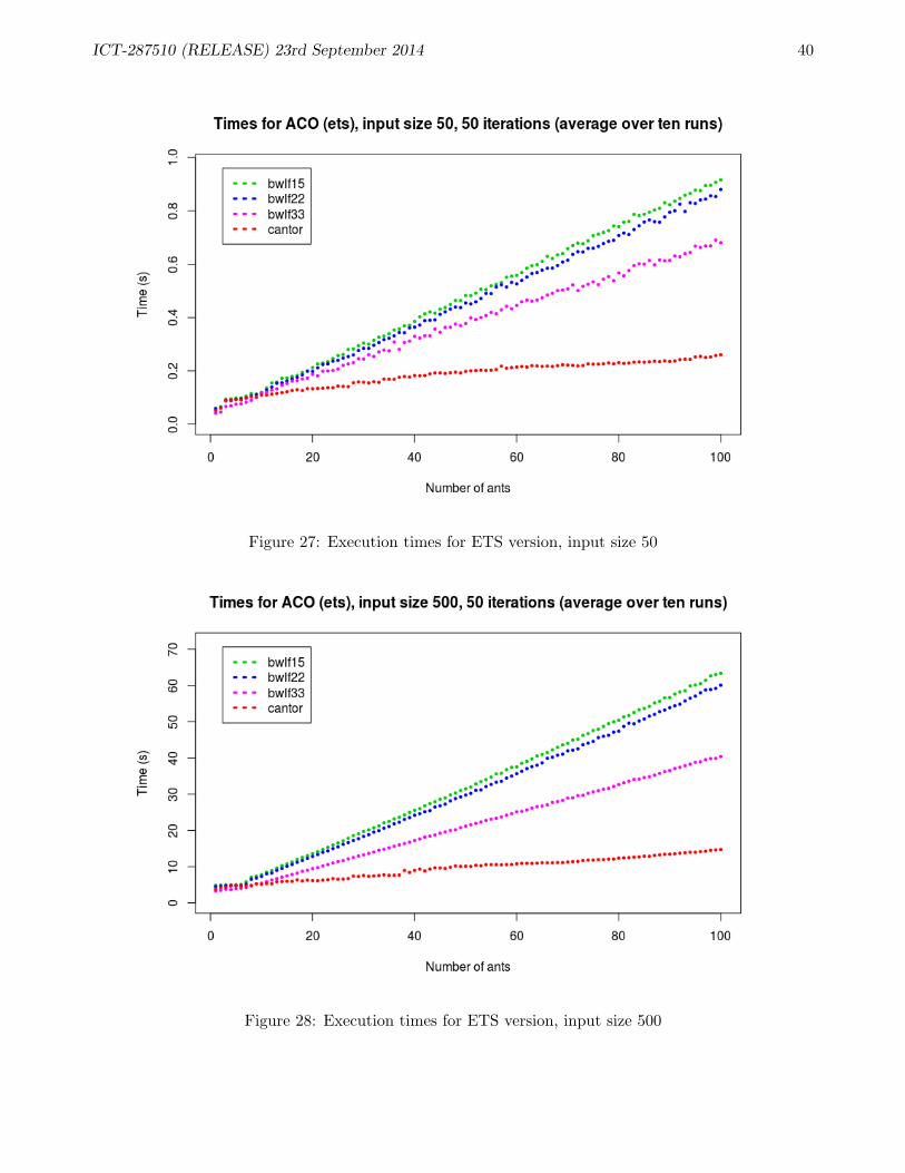
ICT-287510 (RELEASE) 23rd September 2014 40
Figure 27: Execution times for ETS version, input size 50
Figure 28: Execution times for ETS version, input size 500
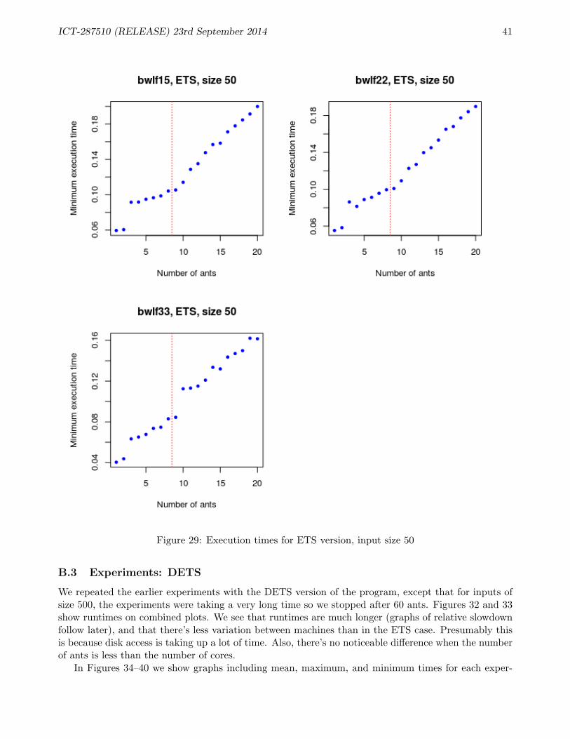
ICT-287510 (RELEASE) 23rd September 2014 41
Figure 29: Execution times for ETS version, input size 50
B.3 Experiments: DETS
We repeated the earlier experiments with the DETS version of the program, except that for inputs ofsize 500, the experiments were taking a very long time so we stopped after 60 ants. Figures 32 and 33show runtimes on combined plots. We see that runtimes are much longer (graphs of relative slowdownfollow later), and that there’s less variation between machines than in the ETS case. Presumably thisis because disk access is taking up a lot of time. Also, there’s no noticeable difference when the numberof ants is less than the number of cores.
In Figures 34–40 we show graphs including mean, maximum, and minimum times for each exper-
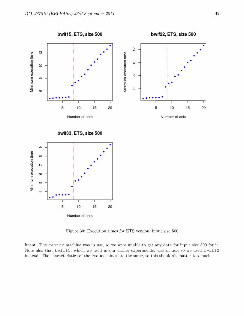
ICT-287510 (RELEASE) 23rd September 2014 42
Figure 30: Execution times for ETS version, input size 500
iment. The cantor machine was in use, so we were unable to get any data for input size 500 for it.Note also that bwlf15, which we used in our earlier experiments, was in use, so we used bwlf12instead. The characteristics of the two machines are the same, so this shouldn’t matter too much.
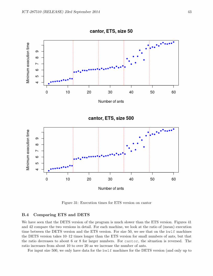
ICT-287510 (RELEASE) 23rd September 2014 43
Figure 31: Execution times for ETS version on cantor
B.4 Comparing ETS and DETS
We have seen that the DETS version of the program is much slower than the ETS version. Figures 41and 42 compare the two versions in detail. For each machine, we look at the ratio of (mean) executiontime between the DETS version and the ETS version. For size 50, we see that on the bwlf machinesthe DETS version takes 10–12 times longer than the ETS version for small numbers of ants, but thatthe ratio decreases to about 6 or 8 for larger numbers. For cantor, the situation is reversed. Theratio increases from about 10 to over 20 as we increase the number of ants.
For input size 500, we only have data for the bwlf machines for the DETS version (and only up to
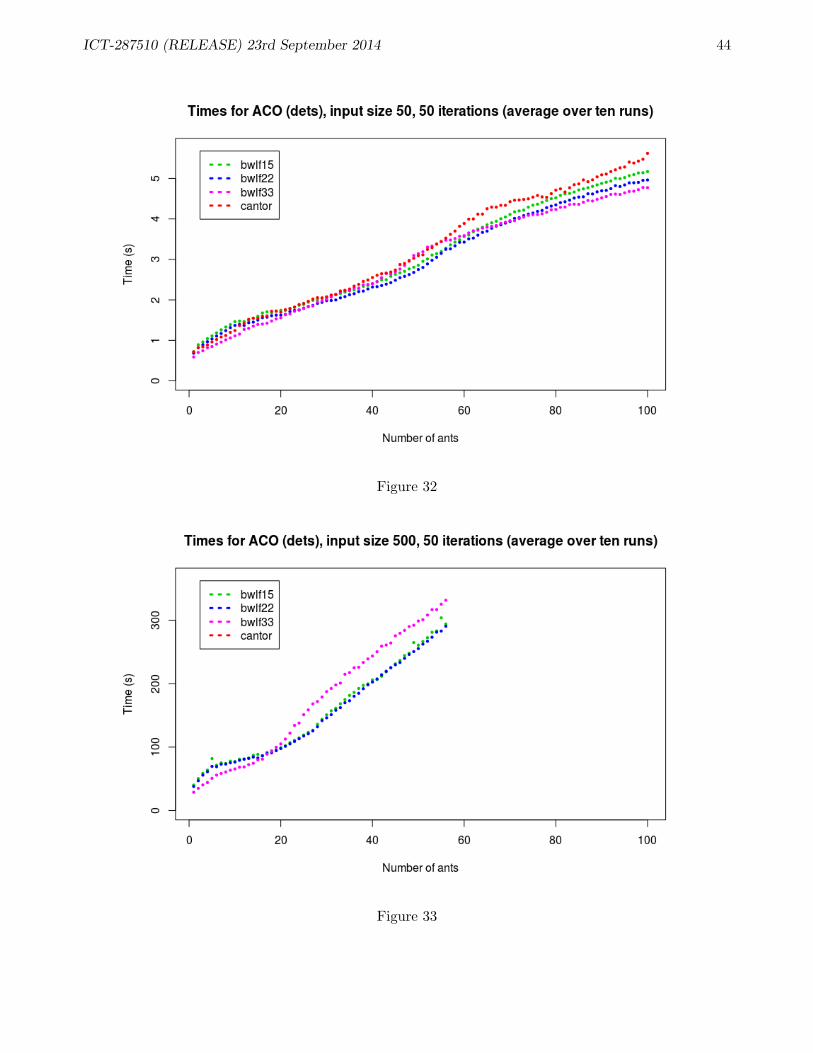
ICT-287510 (RELEASE) 23rd September 2014 44
Figure 32
Figure 33
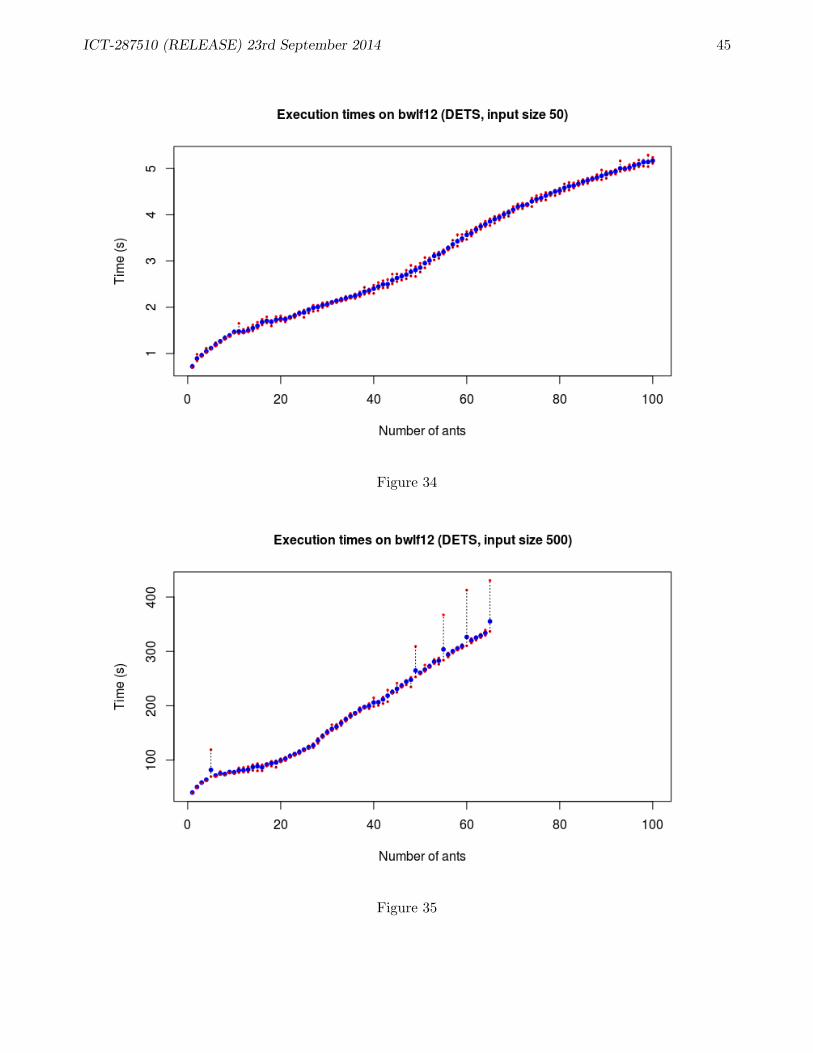
ICT-287510 (RELEASE) 23rd September 2014 45
Figure 34
Figure 35
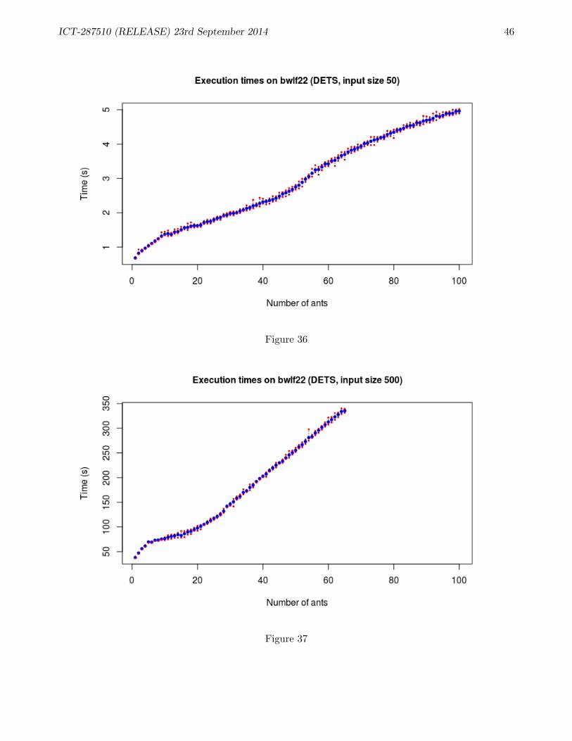
ICT-287510 (RELEASE) 23rd September 2014 46
Figure 36
Figure 37
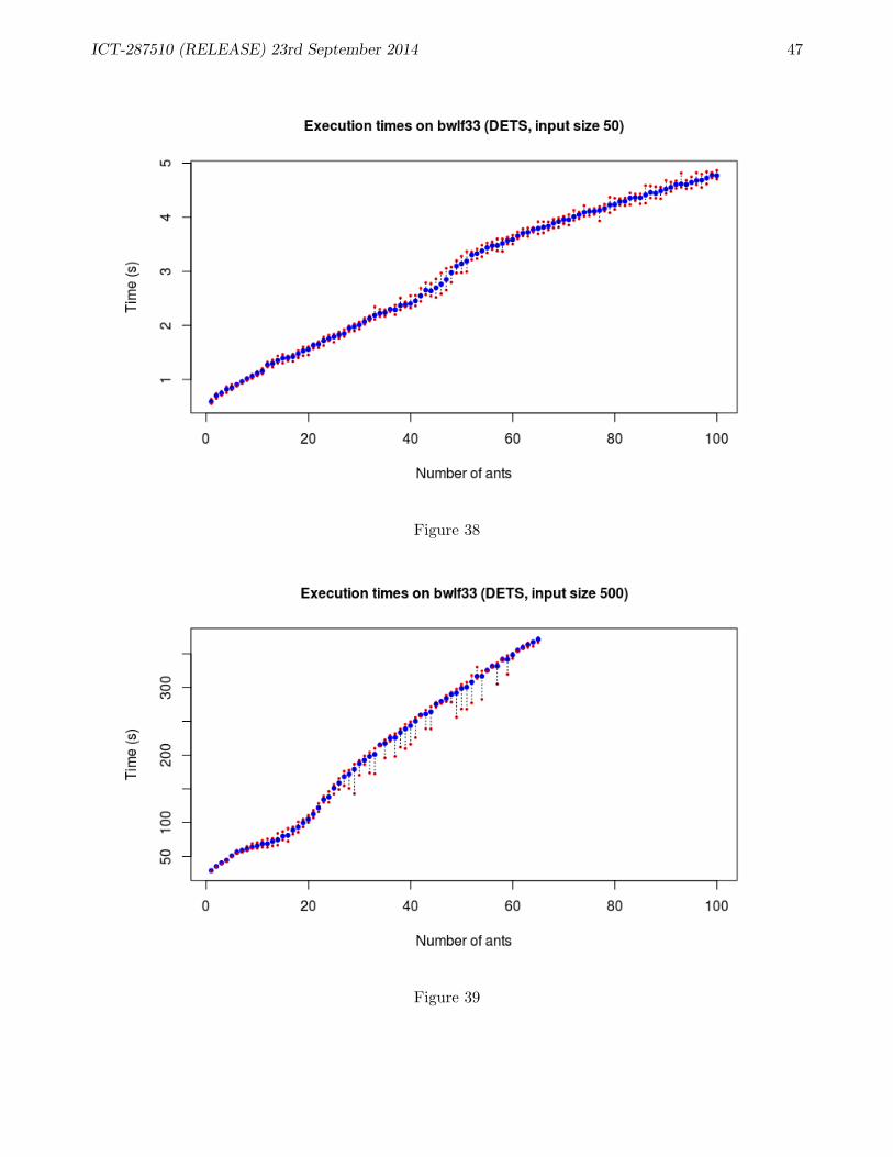
ICT-287510 (RELEASE) 23rd September 2014 47
Figure 38
Figure 39
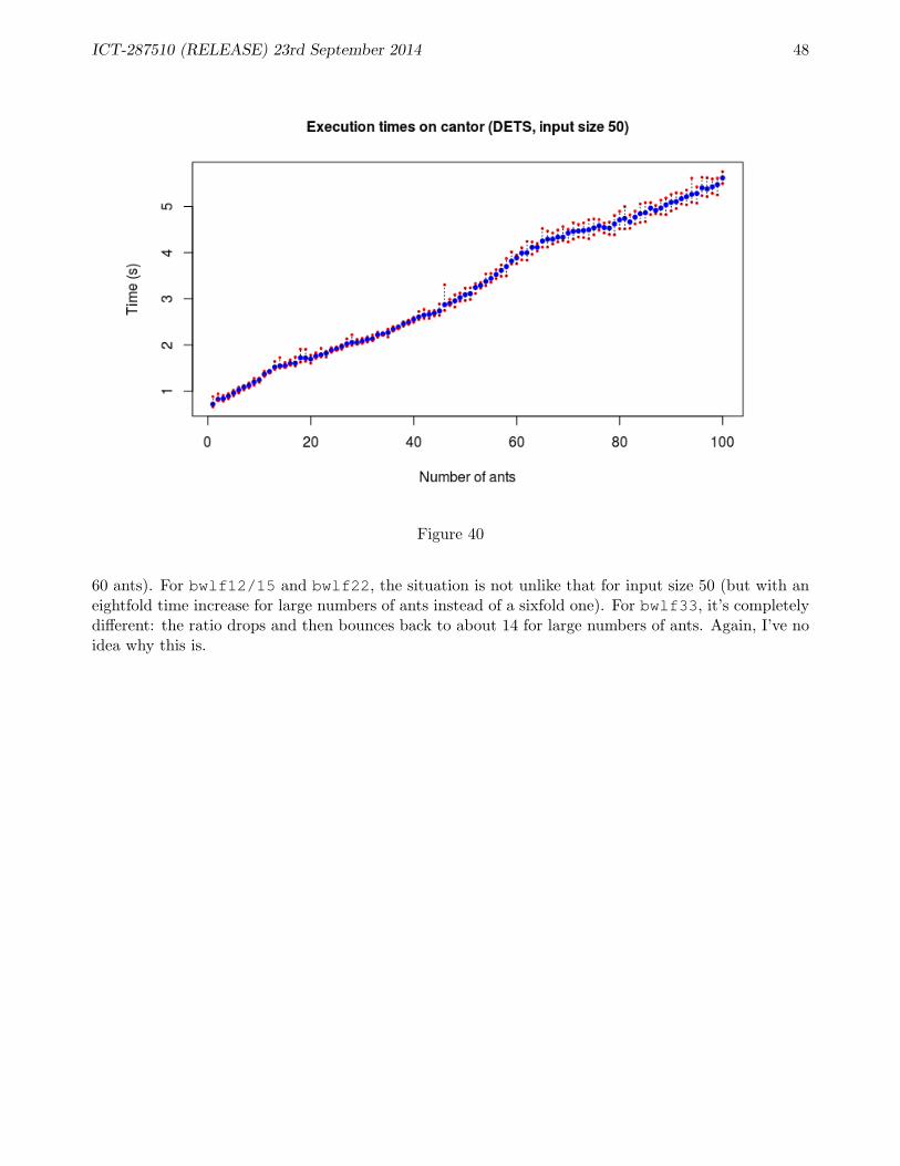
ICT-287510 (RELEASE) 23rd September 2014 48
Figure 40
60 ants). For bwlf12/15 and bwlf22, the situation is not unlike that for input size 50 (but with aneightfold time increase for large numbers of ants instead of a sixfold one). For bwlf33, it’s completelydifferent: the ratio drops and then bounces back to about 14 for large numbers of ants. Again, I’ve noidea why this is.
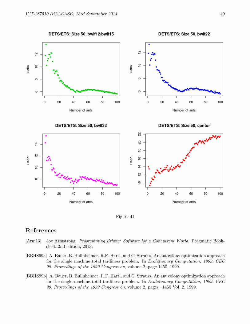
ICT-287510 (RELEASE) 23rd September 2014 49
Figure 41
References
[Arm13] Joe Armstrong. Programming Erlang: Software for a Concurrent World. Pragmatic Book-shelf, 2nd edition, 2013.
[BBHS99a] A. Bauer, B. Bullnheimer, R.F. Hartl, and C. Strauss. An ant colony optimization approachfor the single machine total tardiness problem. In Evolutionary Computation, 1999. CEC99. Proceedings of the 1999 Congress on, volume 2, page 1450, 1999.
[BBHS99b] A. Bauer, B. Bullnheimer, R.F. Hartl, and C. Strauss. An ant colony optimization approachfor the single machine total tardiness problem. In Evolutionary Computation, 1999. CEC99. Proceedings of the 1999 Congress on, volume 2, pages –1450 Vol. 2, 1999.
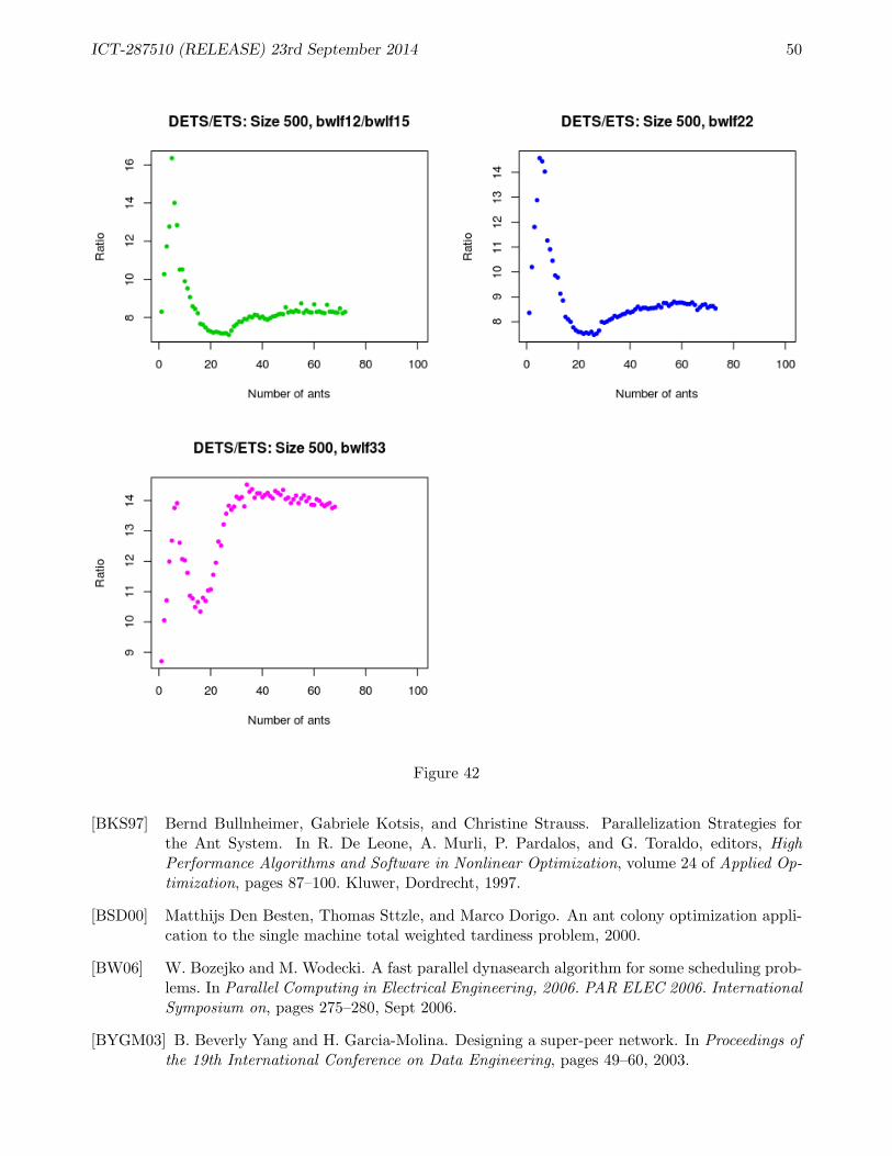
ICT-287510 (RELEASE) 23rd September 2014 50
Figure 42
[BKS97] Bernd Bullnheimer, Gabriele Kotsis, and Christine Strauss. Parallelization Strategies forthe Ant System. In R. De Leone, A. Murli, P. Pardalos, and G. Toraldo, editors, HighPerformance Algorithms and Software in Nonlinear Optimization, volume 24 of Applied Op-timization, pages 87–100. Kluwer, Dordrecht, 1997.
[BSD00] Matthijs Den Besten, Thomas Sttzle, and Marco Dorigo. An ant colony optimization appli-cation to the single machine total weighted tardiness problem, 2000.
[BW06] W. Bozejko and M. Wodecki. A fast parallel dynasearch algorithm for some scheduling prob-lems. In Parallel Computing in Electrical Engineering, 2006. PAR ELEC 2006. InternationalSymposium on, pages 275–280, Sept 2006.
[BYGM03] B. Beverly Yang and H. Garcia-Molina. Designing a super-peer network. In Proceedings ofthe 19th International Conference on Data Engineering, pages 49–60, 2003.
ICT-287510 (RELEASE) 23rd September 2014 51
[CPvdV02] Richard K. Congram, Chris N. Potts, and Steef L. van de Velde. An iterated dynasearchalgorithm for the single-machine total weighted tardiness scheduling problem. INFORMSJournal on Computing, 14(1):52–67, 2002.
[CPvW98] H. A. J. Crauwels, C. N. Potts, and L. N. van Wassenhove. Local search heuristics forthe single machine total weighted tardiness scheduling problem. INFORMS Journal onComputing, 10(3):341–350, 1998.
[CT09] Francesco Cesarini and Simon Thompson. Erlang Programming. O’Reilly Media, Inc., 1stedition, 2009.
[CV14] Francesco Cesarini and Steve Vinoski. Designing for Scalability with Erlang/OTP: Imple-menting Robust, Fault-Tolerant Systems. O’Reilly Media, 2014.
[dBSD00] Matthijs den Besten, Thomas Stutzle, and Marco Dorigo. Ant colony optimization for thetotal weighted tardiness problem. In Marc Schoenauer, Kalyanmoy Deb, Gnther Rudolph,Xin Yao, Evelyne Lutton, JuanJulian Merelo, and Hans-Paul Schwefel, editors, ParallelProblem Solving from Nature PPSN VI, volume 1917 of Lecture Notes in Computer Science,pages 611–620. Springer Berlin Heidelberg, 2000.
[dBSD01] Matthijs den Besten, Thomas Stutzle, and Marco Dorigo. Design of iterated local searchalgorithms. In Egbert J. W. Boers, Jens Gottlieb, Pier Luca Lanzi, Robert E. Smith, StefanoCagnoni, Emma Hart, Gnther R. Raidl, and H. Tijink, editors, EvoWorkshops, volume 2037of Lecture Notes in Computer Science, pages 441–451. Springer, 2001.
[DL90] Jianzhong Du and Joseph Y.-T. Leung. Minimizing total tardiness on one machine is np-hard. Mathematics of Operations Research, 15(3):483–495, 1990.
[DS04] Marco Dorigo and Thomas Stutzle. Ant Colony Optimization. Bradford Company, Scituate,MA, USA, 2004.
[DS10] Marco Dorigo and Thomas Stutzle. Ant colony optimization: Overview and recent advances.In Michel Gendreau and Jean-Yves Potvin, editors, Handbook of Metaheuristics, volume146 of International Series in Operations Research & Management Science, pages 227–263.Springer US, 2010.
[EDF10] EDF. The Sim-Diasca Simulation Engine, 2010. http://www.sim-diasca.com.
[Emm69] Hamilton Emmons. One-machine sequencing to minimize certain functions of job tardiness.Operations Research, 17(4):pp. 701–715, 1969.
[GCTM13] Amir Ghaffari, Natalia Chechina, Phil Trinder, and Jon Meredith. Scalable persistentstorage for Erlang: Theory and practice. In Proceedings of the Twelfth ACM SIGPLANWorkshop on Erlang, pages 73–74, New York, NY, USA, 2013. ACM.
[GDCT04] A. Grosso, F. Della Croce, and R. Tadei. An enhanced dynasearch neighborhood for thesingle-machine total weighted tardiness scheduling problem. Oper. Res. Lett., 32(1):68–72,January 2004.
[Gei09] Martin Josef Geiger. The single machine total weighted tardiness problem – is it (for meta-heuristics) a solved problem ? CoRR, abs/0907.2990, 2009.
[Gei10a] Martin Josef Geiger. New instances for the single machine total weighted tardiness problem.Technical Report Research Report 10-03-01, Helmut-Schmidt-Universitt, Hamburg, March2010.
ICT-287510 (RELEASE) 23rd September 2014 52
[Gei10b] Martin Josef Geiger. On heuristic search for the single machine total weighted tardinessproblem – some theoretical insights and their empirical verification. European Journal ofOperational Research, 207(3):1235 – 1243, 2010.
[HTF01] Trevor Hastie, Robert Tibshirani, and Jerome Friedman. The Elements of Statistical Learn-ing. Springer Series in Statistics. Springer New York Inc., New York, NY, USA, 2001.
[KR90] L. Kaufman and P.J. Rousseeuw. Finding Groups in Data: An Introduction to ClusterAnalysis. Wiley Series in Probability and Statistics. Wiley, 1990.
[KYSO00] H. Kawamura, M. Yamamoto, K. Suzuki, and A. Ohuchi. Multiple Ant Colonies AlgorithmBased on Colony Level Interactions. IEICE Transactions on Fundamentals of Electronics,Communications and Computer Sciences, E83-A(2):371–379, 2000.
[Law77] Eugene L. Lawler. A “pseudopolynomial” algorithm for sequencing jobs to minimize totaltardiness. In B.H. Korte P.L. Hammer, E.L. Johnson and G.L. Nemhauser, editors, Studies inInteger Programming, volume 1 of Annals of Discrete Mathematics, pages 331–342. Elsevier,1977.
[LRKB77] Jan Karel Lenstra, AHG Rinnooy Kan, and Peter Brucker. Complexity of machine schedul-ing problems. Annals of discrete mathematics, 1:343–362, 1977.
[McN59] Robert McNaughton. Scheduling with deadlines and loss functions. Management Science,6(1):1–12, 1959.
[MM98] R. Michel and M. Middendorf. An Island Model Based Ant System with Lookahead for theShortest Supersequence Problem. In A.E. Eiben, T. Back, H.-P. Schwefel, and M. Schoe-nauer, editors, Proceedings of the Fifth International Conference on Parallel Problem Solvingfrom Nature (PPSN V), pages 692–701. Springer-Verlag, New York, 1998.
[MM99] R. Michel and M. Middendorf. An ACO Algorithm for the Shortest Common SupersequenceProblem. In D. Corne, M. Dorigo, and F. Glover, editors, New Ideas in Optimisation, pages51–61. McGraw-Hill, London, UK, 1999.
[MM00] Daniel Merkle and Martin Middendorf. An ant algorithm with a new pheromone evaluationrule for total tardiness problems. In Proceedings of EvoWorkshops 2000, volume 1803 ofLNCS, pages 287–296. Springer Verlag, 2000.
[MRS02] Martin Middendorf, Frank Reischle, and Hartmut Schmeck. Multi colony ant algorithms.Journal of Heuristics, 8(3):305–320, May 2002.
[MRV84] T.E. Morton, R.M. Rachamadugu, and A. Vopsalainen. Accurate myopic heuristics fortardiness scheduling. Technical Report GSIA Working Paper 36-83-84, Carnegie–MellonUniversity, 1984.
[MST13] Patrick Maier, Robert J. Stewart, and Philip W. Trinder. Reliable scalable symbolic com-putation: The design of SymGridPar2. In SAC, pages 1674–1681, 2013.
[PVW91] C. N. Potts and L. N. Van Wassenhove. Single machine tardiness sequencing heuristics. IIETransactions, 23(4):346–354, 1991.
[REL12] RELEASE Project. Deliverable D3.1: Scalable Reliable SD Erlang Design, June 2012.
[REL13a] RELEASE Project. Deliverable D3.2: Scalable SD Erlang Computation Model, July 2013.
ICT-287510 (RELEASE) 23rd September 2014 53
[REL13b] RELEASE Project. Deliverable D3.3: Scalable SD Erlang Reliability Model, September2013.
[REL14a] RELEASE Project. Deliverable D5.3: Systematic Testing and Debugging Tools, June 2014.
[REL14b] RELEASE Project. devo, 2014. http://kar.kent.ac.uk/34968/.
[REL14c] RELEASE Project. Percept2, 2014. http://kar.kent.ac.uk/34875/.
[RL02] Marcus Randall and Andrew Lewis. A parallel implementation of ant colony optimization.Journal of Parallel and Distributed Computing, 62(9):1421–1432, 2002.
[RV09] NR Srinivasa Raghavan and M Venkataramana. Parallel processor scheduling for minimiz-ing total weighted tardiness using ant colony optimization. The International Journal ofAdvanced Manufacturing Technology, 41(9-10):986–996, 2009.
[Spi14] SpilGames. Spapi-router: A partially-connected Erlang clustering, 2014.https://github.com/spilgames/spapi-router.
[TL13] Simon Thompson and Huiqing Li. Percept2, 2013. https://github.com/release-project/midproject-workshop/blob/master/5-Percept2.pdf.


![Erlang/OTP System Documentation · Erlang/OTP System Documentation Erlang (BEAM) emulator version 5.0.1 [threads] Eshell V5.0.1 (abort with ^G) 1> • Start the GS-based toolbar from](https://img.pdfslide.us/doc/110x75/5ea165550a2b94416b7bfc52/erlangotp-system-erlangotp-system-documentation-erlang-beam-emulator-version.jpg)