Embed Size (px)
Citation preview
iTesla Innovative Tools for Electrical System Security within Large Area
Grant agreement number 283012 Funding scheme Collaborative projects
Start date 01.01.2012 Duration 48 months
Call identifier FP7-ENERGY-2011-1
Deliverable D3.1 Part II – Limitations of current modelling
approaches
Dissemination level
PU Public. X
TSO Restricted to consortium members and TSO members of ENTSO-E (including the Commission Services).
RE Restricted to a group specified by the consortium (including the Commission services).
CO Confidential, only for members of the consortium (including the Commission services).
iTesla WP3.2 : Deliverable D3.1 – Part II – Limitations of current modelling approaches V10
1/ 84
Document Name: Limitations of current modelling approaches Work Package: WP3 Task: WP3.2 Deliverable: D3.1 (Part II) Responsible Partner: TE
Author Approval
Name Visa Name Date
[TE] Stijn COLE Task Leader – Stijn COLE (TE)
WP Leader – Dr. Luigi Vanfretti (KTH)
Executive Board
Steering Committee
DIFFUSION LIST
For action For information
All partners All partners
DOCUMENT HISTORY
Index Date Author(s) Main modifications
V1 Aug 17, 2012 S. Cole Draft
V2 Oct 29, 2012 T. Bogodorova, L. Vanfretti 2.1 Section was updated.
V3 Oct 31, 2012 S. Cole Contributions of AIA, RTE, KTH, TE added
V8.1 Feb 14, 2013 Gladys León Marc Sabaté
AIA simulation results
V8.3 Mar 25, 2013 S. Cole Compilation of second round of contributions from AIA, TE, and DTU
V8.4 Mar 27, 2013 S. Cole Conclusions and editing
V9 Mar 28, 2013 S. Cole More editing
V9.1 Apr 8, 2013 S. Cole References DTU added
V9.4 Apr 18, 2013 S. Cole Final version for review after integrating comments from AIA and KTH
V9.5 May 13, 2013 S. Cole Integrating reviewers’ comments
V10 May 27, 2013 S. Cole Final version
iTesla WP3.2 : Deliverable D3.1 – Part II – Limitations of current modelling approaches V10
2/ 84
TABLE OF CONTENTS
1. INTRODUCTION ................................................................................................................................................. 4
2. VALIDATION FLOW CHART .......................................................................................................................... 4
3. LIMITATIONS OF COMMON MODELLING PRACTICES ......... ............................................................... 9
3.1. EQUATION-BASED MODELLING ....................................................................................................................... 9 3.1.1. Introduction ......................................................................................................................................... 10
3.1.2. Input/output or causal Modelling ........................................................................................................ 10
3.1.3. Equation-based modelling: MODELICA ............................................................................................. 10 3.1.4. General comparison ............................................................................................................................ 11
3.1.5. Preliminary Conclusions ..................................................................................................................... 14
3.1.6. Simulations .......................................................................................................................................... 14
3.1.7. Some Specific Limitations of Input/output and Equation-based Modelling ......................................... 21
4. AGGREGATE MODELS ................................................................................................................................... 21
4.1. AGGREGATE MODELS: RATIONALE ............................................................................................................... 21 4.2. WIND POWER AGGREGATION ........................................................................................................................ 22
4.2.1. Methods................................................................................................................................................ 22
4.2.2. Limitations of the wind power aggregation ......................................................................................... 23
4.3. PV POWER AGGREGATION ............................................................................................................................ 24 4.4. LOAD AGGREGATION .................................................................................................................................... 24
4.5. HYBRID SUBSYSTEMS .................................................................................................................................... 25
4.6. CONCLUSIONS ............................................................................................................................................... 26
5. STANDARD MODELS ...................................................................................................................................... 26
5.1. INTRODUCTION .............................................................................................................................................. 26
5.2. STANDARD ELECTRICAL MODELS FOR WIND POWER GENERATION ................................................................. 27 5.2.1. Model specifications ............................................................................................................................ 27
5.2.2. Wind turbine, plant and grid model interfaces .................................................................................... 28 5.2.3. Type 1 models ...................................................................................................................................... 30
5.2.4. Type 2 model ........................................................................................................................................ 30
5.2.5. Type 3 models ...................................................................................................................................... 31
5.2.6. Type 4 models ...................................................................................................................................... 32
5.3. MODELS FOR GAS TURBINES .......................................................................................................................... 33 5.3.1. Controls of Gas Turbines ..................................................................................................................... 33
5.3.2. Overview of Available Standard Models ............................................................................................. 35
5.3.3. Approximations in gas turbine models ................................................................................................. 41
5.3.4. The ALSTOM GT26 Model .................................................................................................................. 44
5.3.5. Comparison of the ALSTOM GT26 Model with Standard Models ...................................................... 44 5.3.6. Gas Turbine Models: Conclusions ....................................................................................................... 47
5.4. CONCLUSIONS ............................................................................................................................................... 47
6. PHYSICAL VS MATHEMATICAL MODELS ................... ............................................................................ 47
7. CONCLUSIONS AND RECOMMENDATIONS ............................................................................................ 47
8. BIBLIOGRAPHY ............................................................................................................................................... 48
9. APPENDIX .......................................................................................................................................................... 50
9.1. APPENDIX A: MODELICA FOR POWER SYSTEM ANALYSIS ............................................................................ 50 9.2. APPENDIX B: POWER SYSTEM LIBRARY ........................................................................................................ 69

iTesla WP3.2 : Deliverable D3.1 – Part II – Limitations of current modelling approaches V10
3/ 84
9.2.1. Electrical blocks .................................................................................................................................. 69
9.2.2. Non-Electrical blocks .......................................................................................................................... 76
9.3. APPENDIX C : NGET’S VALIDATION PROCEDURE ........................................................................................ 78
9.4. APPENDIX D: VALIDATION FLOW CHART ..................................................................................................... 81
iTesla WP3.2 : Deliverable D3.1 – Part II – Limitations of current modelling approaches V10
4/ 84
1. INTRODUCTION The aim of the present document is to identify limitations of common modelling approaches for phasor-based time domain simulation of power systems. It is well known that the phasor paradigm leads to a number of implicit assumptions, such as perfectly sinusoidal signals at the fundamental frequency. However, the focus here is on less obvious approximations and assumptions. The document starts with a flow chart of the validation process of a power system model. The validation process itself is prone to a number of assumptions and approximations. In this document, four common modelling approaches are investigated. The first one is related to the modelling approach of power system equipment. Traditionally, input-output models are used to describe power system equipment. However, equation-based modelling is a new modelling paradigm that could be used for power systems. The second approximation is using aggregated models instead of modelling each constituting element separately. The third simplification is using standard models instead of detailed, custom-made models. Lastly, black-box versus white-box modelling is treated concisely.
2. VALIDATION FLOW CHART In this section, a flow chart for model validation is proposed. The flow chart is primarily intended for validation of complete power system models. Using the flow chart, one can derive in a systematic way all approximations that have been made to arrive at a model. As such, the flow chart can be used to make a list of limitations of common modelling practices. In the flow chart, actions can be suggested. Also, a scoring mechanism could be used to score a certain model. The flow chart can be found in Appendix D, and can be described as:
1) Define the scope of the study • Types of phenomena
o Angular stability (small disturbance, large disturbance) o Frequency stability o Voltage stability (small disturbance, large disturbance) o Other / mix
• Typical spectrum of phenomena o Static / quasi static o Slow dynamics o Fast / transient dynamics o Frequency range (from X to Y Hz)
Limitation(s): • Insufficient definition of the scope of the study may lead to inappropriate choice of
modelling language, model definition, simulation tool and finally to erroneous study conclusions.
2) Define the model Taking into account the scope of the study and the budget available for system modelling: • Analyse the structure of the actual system:
o Size (numbers of substations, power plants, lines, etc.) o Location of main power plants, major loads and industries, tie-lines, etc.
iTesla WP3.2 : Deliverable D3.1 – Part II – Limitations of current modelling approaches V10
5/ 84
o “Shape” (mostly radial, highly meshed, etc.), typical distance between substations, “density” of loads, etc.
• Define the physical extension of the model, considering both the “vertical” extension (i.e. the voltage levels to model) and the “horizontal” extension (i.e. the areas, the countries, etc.):
o Transmission grid, including substations o Power plants, including auxiliaries and controllers / governors o Loads / feeders o External / equivalent networks if any / needed o Automatons / relays
• For each component, define also the required level of detail. Decide: o Which components must be modelled individually o Which components can be aggregated (clusters, equivalent model)
• For each component, define which model type / structure is available / suitable: o Linear model o Non-linear model o Input – output model o Equation based model o Neural network model o Black-box model (including DLL from manufacturer) o Physically parameterised model
� Standard (e.g. IEEE) � Custom
• Detailed • Simplified
o Model including digital controllers Limitation(s): • Insufficient analysis of the actual system may cause inappropriate decision in modelling,
for instance: o Inclusion of areas, voltage levels or components which are not relevant for the
study, resulting in a bigger model, with potentially more uncertainties on structure and parameters (this is a type of “false precision”).
o Exclusion or aggregation of relevant areas, voltage levels or components, causing a loss of model accuracy.
• Poor characterisation of the model type / structure for each component may cause inappropriate choice with respect to:
o The scope of the study (see 1). For instance: � Use of linear model to study highly non-linear phenomena, � Use of simplified models where details are needed.
o The modelling language or the simulation tool (see 3). This is especially the case if model types are:
� Equation based, mainly if including discrete equations / variables, � DLL from manufacturer, � Digital controllers.
3) Select modelling language and simulation tool Taking into account: • The scope of the study • The selected model If there is no adequate modelling language and/or simulation tool, restrict the scope of the study and/or revise the model Limitation(s): • Inappropriate modelling language will not allow implementing the selected model (see
2).
iTesla WP3.2 : Deliverable D3.1 – Part II – Limitations of current modelling approaches V10
6/ 84
• Inappropriate simulation tool will not allow proper simulation of the designed model, causing for instance numerical instabilities if not execution errors. Each simulation tool has capabilities and limitations, for instance ability to cope with equation based models, or to connect DLLs from manufacturers, or deal with small time constants, etc.
4) Build model • List data (parameters) needed for each component of the model • Check availability of parameters
o From previously completed / validated models and similar studies o From manufacturers o From measurements o From database available for the study (from customer for instance) o From similar component o From estimation o From good practice / default value o Etc.
• Check also whether parameters have been regularly used or have been updated recently. • Evaluate suitability of available parameters:
o Derive a score for models: � Data from measurement campaigns are better than estimated
parameters… � Regularly updated data are better than “old” data…
o If deemed not suitable (insufficient score): � Consider data collection � Revise the model
Limitation(s): • Models with a poor quality can contaminate all simulation results. In a sense it is better to
have a simple model with proven parameters than a complex model based on dubious data (assuming here that limitations of simple models are known and compatible with the scope of the study).
• Scoring of model could lead to inadequate decision if not properly tuned. We must be aware that a model can be good for one thing (for instance long-term dynamic) and bad for another thing (for instance short-term dynamic). In other words, scoring must take into account the scope of the study (i.e. the phenomena to analyse, see 1). More generally,
o If the scoring process is too optimistic, inadequate models could be accepted and lead to poor simulation results,
o If the scoring process is too pessimistic, it could be decided to perform an additional data collection and/or to revise the model although it was not needed, which is costly.
5) Validate the static model • Elementary checks: detect abnormal parameters by comparison to typical values, for
example o 1/SQRT(l*c) ≈ 300000 km/sec for lines o Ucc ≈ 0.1 pu for transformers o “Three Sigma Rule”, i.e. the rule that in a normal distribution, most values are
within 3σ of the mean, if applicable o Etc.
• Check initial state for simulations: generally supposed to be a “normal” state o Check convergence of the solution (poor convergence can reveal parameter
issues) o Voltages ≈ 1 pu o Flows < rated MVA o No tap numbers at minimum or maximum
iTesla WP3.2 : Deliverable D3.1 – Part II – Limitations of current modelling approaches V10
7/ 84
o P and Q of generators within the limits and/or inside the capability curves o Check N- 1 criteria for the model o Check short circuit currents / powers (Pcc) for the model o Check computed state against the measurements at start of recordings if available o Run an OPF to improve the system state if needed or to compensate lack of
information about the actual state Limitation(s): • Elementary checks are necessary but not sufficient! • In case the initial state cannot be univocally identified from references (which is often the
case when the number of available measurements is limited), dealing with uncertainties is subject to assumptions. Depending on the chosen assumptions, the calculated state can range from best to worst (from ideally optimised state to worst case approach), with strong consequences on the simulations. In some cases, considering a normal state is too optimistic and does not reflect the actual situation at the start of study / scenarios to investigate.
6) Validate the dynamic model • Elementary checks: detect abnormal parameters by comparison to typical values, for
example o Typical order of magnitude of electrical parameters, time constants, etc. o “Three Sigma Rule” rule if applicable o Etc.
• Check initial state for simulations: generally supposed to be a “steady” state o Variables that are out of range or at their limits o Variables that are not at equilibrium
• Qualitative validation: o Small signal analysis:
� Excite inter-area modes � Compute eigenvalues � Check whether the system is small-signal stable � Check whether frequencies and damping factors of modes are typical for
the system o Simulate typical scenarios like
� Steady state (scenario without events) � Short-circuits � Modifications of set-point values � Partial / total load rejection � Check typical stability margins (critical clearing time or other stress
margin to collapse) Analyse time domain behaviour of the system for those typical scenarios and check if it looks “normal”. Check also if there is no numerical instability caused by the model / simulation tool
• Quantitative validation: check simulated behaviour against measurements o Analyse available measurements
� Evaluate accuracy � Filter noise � Filter harmonics � Correct possible errors like measurement bias / offset � Process data as needed as for performance indicators (for instance
evaluate measured modes) o Define adequate performance indicators and detection thresholds
� The performance indicator requires in one form or another a quantification of the difference between two curves. This could be based on the normalised root mean square deviation (NRMSD).
iTesla WP3.2 : Deliverable D3.1 – Part II – Limitations of current modelling approaches V10
8/ 84
� Consider performance indicators that are valid • For the duration of the whole simulation • On a time interval (window) of the simulation • At each time of the simulation (for instance distance between the
measured curves and the simulated curves) � For each type of phenomena, one or more performance indicators are
defined. o Create validation scenarios containing the sequence of events during the period
of the measurements, provided that the scenarios are compatible with the model (e.g. short circuit scenario versus model valid for long term dynamics)
o Run simulations and compute performance indicators Limitation(s): • Elementary checks are necessary but not sufficient! • Small signal analysis is based on system linearization at a given operational state
(generally the initial state from 5). The output of small signal analysis would differ if another system state is considered.
• Proper evaluation of typical scenarios requires a high-level expertise in system dynamics. • Definition of performance indicators is subjective to particular contexts. There are two
options: o Either the performance indicators are above the thresholds and discrepancies
must be analysed (see 7), o Or the performance indicators are below the thresholds. In this case, this means
that the indicators do not reveal discrepancies for the given system state(s), model and scenario(s). Having good indicators does not mean that the model is good for everything, another system state or another scenario of the same system! Performance indicators must be carefully chosen, given the scope of the study (i.e. the phenomena to analyse, see 1) and the scenarios used as reference (scenarios used as reference must reflect the ones that will be investigated during the study. For instance, power oscillation reference scenarios are of little interest to validate a model designed to study voltage collapse problems). NB: it is assumed here that the available measurements / references are “error free”.
7) Adapt the model If there are noticeable discrepancies (i.e. detection thresholds are violated): • Reduce the complexity of the analysis
o By determining the relevant geographical zone o By determining whether the discrepancies are related to a specific type of
phenomena (voltage, frequency, etc.), o By determining whether the discrepancies are related to a specific model
• Check whether discrepancies are observed 1) At the initial point of the simulation on
a. Static variables b. Dynamic variables
2) During the whole simulation 3) During some intervals of the simulation 4) From a point / event in the simulation 5) To a point / event in the simulation 6) Increasingly during the simulation
• Evaluate main cause: o Static model / state?
If discrepancies 1a, 2 are observed, and less likely if discrepancy 5 is observed. o Dynamic model / state?
iTesla WP3.2 : Deliverable D3.1 – Part II – Limitations of current modelling approaches V10
9/ 84
If discrepancies 1b, 2, 3, 4, 5 are obsered, and less likely if discrepancy 6 is observed.
o Validation scenarios? If discrepancyies 2, 3, 4, 6 are observed, and less likely if discrepancy 5 is observed
o Measurements? If discrepancies 1, 2, 6 are observed, and less likely if discrepancies 3, 4, 5 are observed
• If the problem is in the dynamic model: o If measurements are available, it is possible to determine which parameters in the
model will be observable (= observability analysis) o Use an impact matrix to determine which models, control loops and parameters
exhibit the highest sensitivity with respect to a given performance indicator (= controllability analysis) Care should be taken when evaluating sensitivities in the presence of non linear functions, limiters, dead bands, logical variables, etc.
• Cross check observability analysis and controllability analysis to select models and control loops to update
• Update selected parameters o By collecting new information o By evaluating their influence on the performance indicators o By optimisation process if possible (= minimisation / maximisation of the
performance indicators) • When update is over, redo validation Limitation(s): • We tried here to systematise the process of adapting the model. It is clear that analysis
and decisions to take rely greatly on a high-level expertise. The steps described here are mainly intended to reduce the complexity of the problem and to help identifying which parts of the process could be assisted (by computations or by computer aided decision support system). Another possible output is the mapping of the parts of the system that were successfully validated and the ones that were not satisfyingly validated.
National Grid Electricity Transmission’s (NGET) main contribution to this task is to detail their internal validation procedure of equipment models and of the complete power system model. It can be found in Appendix C.
3. L IMITATIONS OF COMMON MODELLING PRACTICES
3.1. Equation-based Modelling
In the following section, the main differences between equation-based modelling techniques and modelling based on input-output relations will be presented. Limitations of equation-based modelling techniques with respect to input-output-based modelling are investigated, as well as comparison of simulation results. Because MODELICA is the equation-based modelling language of choice in iTESLA, the analysis is based on this language.
iTesla WP3.2 : Deliverable D3.1 – Part II – Limitations of current modelling approaches V10
10/ 84
3.1.1. Introduction
Numerous reasons can be listed for using equation-based modelling, and simulation software supporting it, instead of input-output modelling, and this is one of the purposes of this section. First of all because in equation-based modelling component models are in most cases open for modification, and secondly because equation-based modelling of components defined in a common language, allows in principle having unambiguous model exchange between different simulations modelling tools without loss of information about the model. For these and many other reasons this section is dedicated to present a detail comparison between equation-based and input/output modelling making especial emphasis in the advantages or disadvantages of each one.
3.1.2. Input/output or causal Modelling
Input/output modelling is based in causal modelling, which consists of a set of relations between variables, inputs and outputs, whereby the data flow from input to output is fixed. Such a model can be represented by a block-diagram with oriented blocks connected by arrows.
Input/output modelling is the dominating standard in power system simulation. Several commercial tools for the simulation of power systems have been developed in the last decades, e.g., PSS/E, EUROSTAG, Simpow, Power System Tools, etc. All of them use the causal modelling paradigm. In the iTESLA project, EUROSTAG is the standard tool for power system modelling and simulation using the causal modelling approach.
A disadvantage of these tools is their closed architecture: the user is not allowed to view or change most of the component models. In some tools such as EUROSTAG, the user has the possibility of modelling complicated controllers such as governors and exciters using block diagram representation, and has access to all block diagrams of the standard models, but cannot modify the network or generator equations. In some other tools, such as Simpow, it is actually possible to change the network equations. Some of these tools have the capability of exporting a linearized representation of the systems for further analysis but the full non-linear representation remains hidden to the user. In other words, beyond a certain point, the implementation is completely hidden, which is not the case in most equation-based modelling tools.
It is difficult to exchange models when using different closed architecture tools. The common strategy nowadays is to use standard models, and to exchange the parameter sets. But as the implementation of the model in different tools can be slightly different, it is necessary to inter-validate the models.
3.1.3. Equation-based modelling: MODELICA
Equation-based modelling defines an implicit relation between variables. The data-flow between variables is not a part of the model: it is defined right before simulation of the model. A system is described in terms of differential-algebraic equations, as is the case in input-output modelling. The system can be seen as a complete model or a set of individual components, each one represented by a set of equations and its
iTesla WP3.2 : Deliverable D3.1 – Part II – Limitations of current modelling approaches V10
11/ 84
corresponding variables. This is done in a general modelling language that can be applied to various application domains1. One of the most important advantages of equation-based modelling is that the user is in principle only concerned with the model creation, and does not have to deal with the underlying simulation engine, although he has the possibility to do this if so desired. It also allows decomposing complex systems into simple sub-models easier to understand, share and reuse, and enables a better model validation, because certain components can be checked individually for consistency. For these reasons and many others that will be explained in the next section, several equation-based modelling languages have been developed since 1960’s, but many of them were not able to prevail outside their original application domain. But the need for a general equation-based modelling language was evident; leading to the creation of a standard modelling language in the 1990’s called MODELICA. MODELICA, as defined by its developers [1], is an object-oriented language for modelling large, complex and heterogeneous physical systems. It allows specification of mathematical models of component-based systems form mechanical, electrical, electronic, hydraulic, fluid, thermal, control, electric power and other domains, with the aim of performing dynamic computer simulations.
The design of Modelica started in September 1996 within an action of the ESPRIT project "Simulation in Europe Basic Research Working Group (SiE-WG)". The first version used in actual applications was finished in December 1999. Since then, many improved versions had been release by the Modelica Association, a non-profit organization based in Linköping Sweden, in charge of the development of the Modelica language [1].
3.1.4. General comparison
In this section, some general advantages and disadvantages of input/output and equation-based modelling are given. In the following, we will focus on MODELICA for equation-based modelling and EUROSTAG for causal modelling because those will be the tools used in this project. However it seems that most of the advantages and disadvantages listed for MODELICA are applicable to other equation-based modelling approaches as well and those for EUROSTAG are true for most other traditional power system simulation software. Were applicable, known differences with other tools are mentioned. Advantages of equation-based modelling
1. Modelica allows creating acausal models that can adapt to more than one data flow context, they support better reuse and exchange of modelling and design knowledge than traditional classes [2]. These model components can be either elementary components (if at the bottom level of the hierarchy), or a composition of other model components.
2. Modelica also allows implementing causal modelling as in the case for the models needed in control systems.
3. The algorithm used by the numerical solver is provided by an appropriate compiler of the Modelica language. The dependencies between input/output variables are established during the compilation
1 For an Equation-based modeling review, see for example Zimmer’s PhD thesis http://www.inf.ethz.ch/personal/cellier/PhD/zimmer_phd.pdf
iTesla WP3.2 : Deliverable D3.1 – Part II – Limitations of current modelling approaches V10
12/ 84
of models and therefore, the modelling and numerical simulations are two completely decoupled steps. Hence, the model is independent from the solver, allowing different solvers to solve the same model.
4. Modelica offers the possibility to develop independent libraries of physical components, which are easily re-used due to this separation of the simulation package.
Disadvantages of equation-based modelling
1. Equation-based models can be harder to simulate for the simulator engine, increasing the time of simulations compare to input-ouput tools. The simulation engines can be improved to cope with specific domain problems, particularly, in the case of the OpenModelica compiler which offers users accesibility to the source code of the simulation engine. Moreover, so-called ‘flat files’ have to be built from the input files before they can be integrated, which is a process that is not needed in power system tools.
2. Because it is a language that has been developed in the last decade, there are still many points that need to be reviewed and improved, such as: existing bugs in open source tools, code generation that can be easily exchanged between different environments, definition of a standard process to define element blocks and create models, etc.
3. The Modelica language has been tested in many small to medium systems, but its scalability to large systems as power systems grid needs to be evaluated. However, large scale systems in other domains (e.g. robotics) have shown that Modelica is suitable for large scale simulations.
4. Due to the numerous environments for editing Modelica and running simulations, existing in the market (open source and commercial), the model exchange between these tools is not really straightforward because each one has different processes to define elements, initialize variables, compile, simulate and show results. This could be due to the limited experience we have had in iTESLA.
5. In numerous cases, the initial values for variables need to be calculated or estimated with other tools in order to initialize a system because the simulator is not able to solve the initialization problem. However, this is only because currently no power flow tool has been developed in Modelica.
Advantages of input/output modelling
1. Scalability. Tools such as EUROSTAG, DIgSILENT and PSS/E can solve very large, complex power systems in an efficient way.
2. Input/output modelling is the standard for power systems. It has been proven and used for decades. Consequently, there is much experience in the use of these tools
3. Very well-suited to power system analysis: it is not difficult to find an input/output model for controls.
Disadvantages of input/output modelling
1. Difficult to exchange models. Exchanging models is a matter of exchanging parameter sets for standard models. However, the equations themselves cannot be exchanged because they are not always available or accessible.
2. In general, input/output block diagrams are less flexible. The user is limited to the fundamental blocks that are available in the tool. Moreover, the network and machine equations are fixed in most tools, so the user cannot change them.
iTesla WP3.2 : Deliverable D3.1 – Part II – Limitations of current modelling approaches V10
13/ 84
There are other disadvantages that are often mentioned in relation to input/output modelling, such as limited reusability, difficulty of modelling equation-based systems, etc., but they seem less relevant to power systems, where the input-output relation is always fixed.
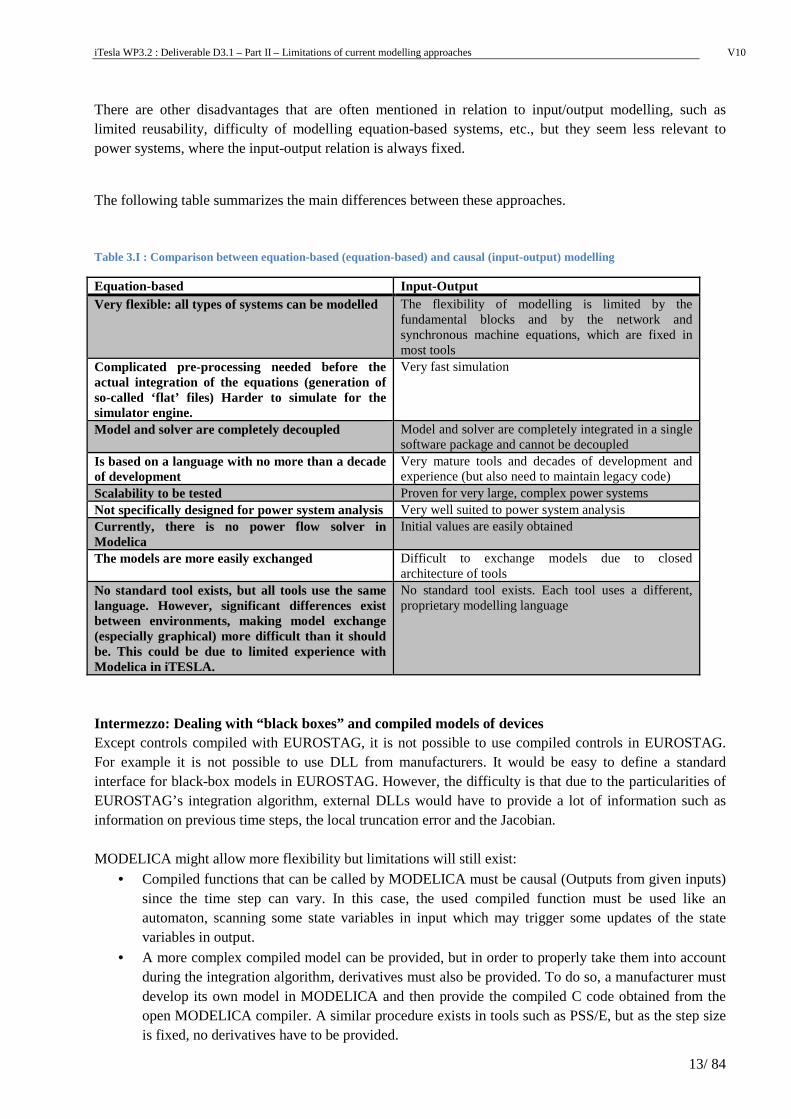
The following table summarizes the main differences between these approaches. Table 3.I : Comparison between equation-based (equation-based) and causal (input-output) modelling
Equation-based Input-Output Very flexible: all types of systems can be modelled The flexibility of modelling is limited by the
fundamental blocks and by the network and synchronous machine equations, which are fixed in most tools
Complicated pre-processing needed before the actual integration of the equations (generation of so-called ‘flat’ files) Harder to simulate for the simulator engine.
Very fast simulation
Model and solver are completely decoupled Model and solver are completely integrated in a single software package and cannot be decoupled
Is based on a language with no more than a decade of development
Very mature tools and decades of development and experience (but also need to maintain legacy code)
Scalability to be tested Proven for very large, complex power systems Not specifically designed for power system analysis Very well suited to power system analysis Currently, there is no power flow solver in Modelica
Initial values are easily obtained
The models are more easily exchanged Difficult to exchange models due to closed architecture of tools
No standard tool exists, but all tools use the same language. However, significant differences exist between environments, making model exchange (especially graphical) more difficult than it should be. This could be due to limited experience with Modelica in iTESLA.
No standard tool exists. Each tool uses a different, proprietary modelling language
Intermezzo: Dealing with “black boxes” and compiled models of devices Except controls compiled with EUROSTAG, it is not possible to use compiled controls in EUROSTAG. For example it is not possible to use DLL from manufacturers. It would be easy to define a standard interface for black-box models in EUROSTAG. However, the difficulty is that due to the particularities of EUROSTAG’s integration algorithm, external DLLs would have to provide a lot of information such as information on previous time steps, the local truncation error and the Jacobian. MODELICA might allow more flexibility but limitations will still exist:
• Compiled functions that can be called by MODELICA must be causal (Outputs from given inputs) since the time step can vary. In this case, the used compiled function must be used like an automaton, scanning some state variables in input which may trigger some updates of the state variables in output.
• A more complex compiled model can be provided, but in order to properly take them into account during the integration algorithm, derivatives must also be provided. To do so, a manufacturer must develop its own model in MODELICA and then provide the compiled C code obtained from the open MODELICA compiler. A similar procedure exists in tools such as PSS/E, but as the step size is fixed, no derivatives have to be provided.
iTesla WP3.2 : Deliverable D3.1 – Part II – Limitations of current modelling approaches V10
14/ 84
3.1.5. Preliminary Conclusions
The differences between input/output and equation-based modelling for power systems have been discussed in a qualitative way. It can be roughly concluded at this point that MODELICA has potential for power system simulation in that it allows for easier model exchange and great modelling flexibility. The main barriers to wide-scale use of MODELICA for power system simulation are performance for large systems, and the difficulty of obtaining initial conditions. Models being explicitly defined using easily exchangeable equations, move the focus from putting questions on the “quality of the model” as seen from expected simulation results, to the “quality of the solvers” used by each simulation platform. If the model is well defined and the simulations carried out in different software do not match to measured responses, this could imply that while the model is correct the particular simulation platform giving unexpected results might have difficulties simulating the model, i.e. the solver is not capable to solve the model correctly.
3.1.6. Simulations
Earlier work (PEGASE) In an effort to demonstrate the capability of dealing with an open modelling approach, part of the European Project PEGASE [http://www.fp7-pegase.eu/] (Pan European Grid Advanced Simulation and State Estimation) was dedicated to develop an open simulation and model sharing framework using Modelica language interfaced with Scilab/Xcos environment to model an entire power system. They use SciLab/Xcos platform to create Modelica components, assemble them into models and simulate the models [Pegase. (s.f.). D5.2]. They compare the simulations results with the same model computed in Eurostag, obtaining similar results. The main difficulties encountered in the Pegase project were related to the initialization phase, because the initial values for the differential equations had to be obtained running Eurostag’s power flow and because the approach of Modelica models in Xcos used in this study is not appropriate for modelling blocks whose parameters depend on initial values [Pegase. (s.f.). D5.2].
Power Systems Library and Simulations A power system library was developed in Modelica using the Dymola editing and simulation environment. New component blocks were created in Modelica and many of the power systems components built in Scilab/XCos during the Pegase project were reused. Thanks to this library, time domain simulations of power systems composed of synchronous machines with regulator blocks, transmission lines, transformers, impedance loads, etc., and introducing time events as load increase, line opening, faults, etc. can be performed Each component block contained in the Power Systems library from PEGASE was converted from XCOS/SciLab environment to Dymola, which is a more friendly-user environment that allows the editing and simulation of Modelica models without the need of interface functions, as is the case for XCos/SciLab tool. The following blocks were converted from XCOS/SciLab environment to Dymola:
• PwLine • PwLoad • PwTransfomer • PwFault • PwVoltage • PwCurrent • PwActivePower • PwReactivePower • ImConverterIm
iTesla WP3.2 : Deliverable D3.1 – Part II – Limitations of current modelling approaches V10
15/ 84
• ImConverterEx • ImSetPoint • ImLimitedIntegrator • ImIntegrator • ImLeadlag • ImSum1 • ImSum2 • ImSum3 • ImSum5 • ImMult1 • ImMult2 • ImMult3 • ImStep • ImLimiter • ImVariableLimiter • ImDelay • ImDerivativeLag • ImSimpleLag • ImDeadBand • ImGain • ImCosine • ImSine • ImArcTangent • ImAnd • ImAbs • ImRelay
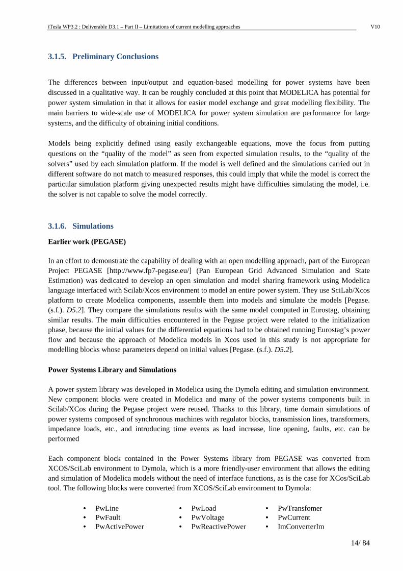
For the Dymola library development, the Modelica models or classes corresponding to each electrical or mathematical block from PEGASE library were imported to Dymola and adapted to the simulation environment, and a graphical part was associated to each component in order to facilitate the construction of electrical system networks just by drawing connections between the corresponding blocks. The Power System library has also been improved adding numerous electrical and mathematical blocks shown in the annex, with the objective to build and simulate different small to medium size power systems built in Dymola and Eurostag, perform time-dependent simulations and validate results with Eurostag. In Appendix B the Modelica model for each component of the Power System library is described, paying special attention to the new models that have been recently developed within the iTesla project. In order to validate the new components created and those translated from Scilab/XCos to Dymola, the results from Pegase were first reproduced in Dymola and then, two new systems were built. In the following, these two systems of power networks will be presented: a system with one machine (“system A”), and another (“system B”) containing two machines (alternating machines given by its external parameters and machines given by its internal parameters, and with or without internal transformers), and we will compare the simulations for both systems with the corresponding Eurostag’s simulations. System A The first system built, shown in the figure, is called System A (Figure 3.1). This system is composed by a 1000 MW unit, a Eurostag synchronous machine defined by its external parameters, feeding a 600 MW 200 Mvar load localized at the 158 kV level through a 24/400kV step-up transformer, two 400 kV lines and a 400/158 kV transformer. Two events are simulated at specific times to study the system behaviour after:
• An instantaneous increase in load of 50 MW 25Mvar at time t = 10s.
• Switching off one of the two 400 kV lines at the receiving node at time t = 20s.
iTesla WP3.2 : Deliverable D3.1 – Part II – Limitations of current modelling approaches V10
16/ 84
Figure 3.1 Dymola diagram of System A
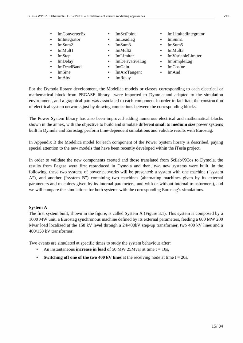
The Eurostag synchronous machine (Generator M2S) is given by its external parameters and a block internally computes the internal parameters. It is equipped with a voltage regulator chain that consists of a constant excitation voltage (EFD), and a governor chain, represented in Figure 3.2.
Figure 3.2 : Dymola diagram of governor GOVER1
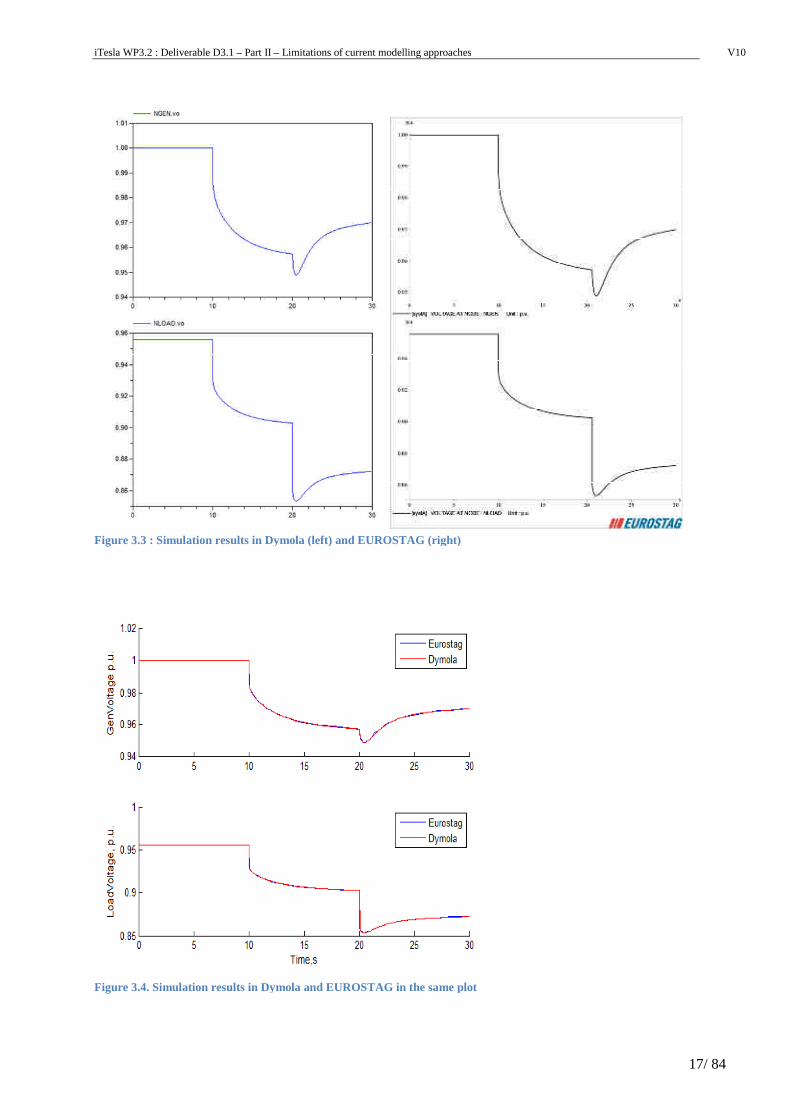
In order to validate system A, the same system must be built and simulated in Eurostag, especially to obtain the initial values necessary for time simulations. The parameters calculated by the power flow computations in Eurostag provide initial values for the synchronous machines models, voltage regulators, turbine governors and loads. Once these values are known, the system can be initialized and run with the Dymola simulator. After running the simulation on Eurostag and Dymola, we obtain the following voltage magnitude output for the NGEN and the NLOAD nodes, with the voltage drop and the subsequent voltage stabilization after an instantaneous increase in load of 50 MW 25Mvar at time t=10s, and after switching off one of the two 380 kV lines at the receiving node at time t = 20s. The results are shown in Figure 3.3, and the results in the sameplot are shown in Figure 3.4.
iTesla WP3.2 : Deliverable D3.1 – Part II – Limitations of current modelling approaches
Figure 3.3 : Simulation results in Dymola (left) and EUROSTAG (right)
Figure 3.4. Simulation results in Dymola and EUROSTAG in the same plot
Limitations of current modelling approaches
: Simulation results in Dymola (left) and EUROSTAG (right)
Simulation results in Dymola and EUROSTAG in the same plot
V10
17/ 84
iTesla WP3.2 : Deliverable D3.1 – Part II – Limitations of current modelling approaches V10
18/ 84
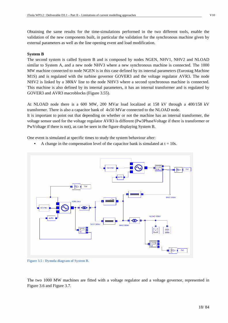
Obtaining the same results for the time-simulations performed in the two different tools, enable the validation of the new components built, in particular the validation for the synchronous machine given by external parameters as well as the line opening event and load modification. System B The second system is called System B and is composed by nodes NGEN, NHV1, NHV2 and NLOAD similar to System A, and a new node NHV3 where a new synchronous machine is connected. The 1000 MW machine connected to node NGEN is in this case defined by its internal parameters (Eurostag Machine M1S) and is regulated with the turbine governor GOVER3 and the voltage regulator AVR3. The node NHV2 is linked by a 380kV line to the node NHV3 where a second synchronous machine is connected. This machine is also defined by its internal parameters, it has an internal transformer and is regulated by GOVER3 and AVR3 macroblocks (Figure 3.55). At NLOAD node there is a 600 MW, 200 MVar load localized at 158 kV through a 400/158 kV transformer. There is also a capacitor bank of 4x50 MVar connected to the NLOAD node.
It is important to point out that depending on whether or not the machine has an internal transformer, the voltage sensor used for the voltage regulator AVR3 is different (Pw3PhaseVoltage if there is transformer or PwVoltage if there is not), as can be seen in the figure displaying System B. One event is simulated at specific times to study the system behaviour after:
• A change in the compensation level of the capacitor bank is simulated at t = 10s.
Figure 3.5 : Dymola diagram of System B.
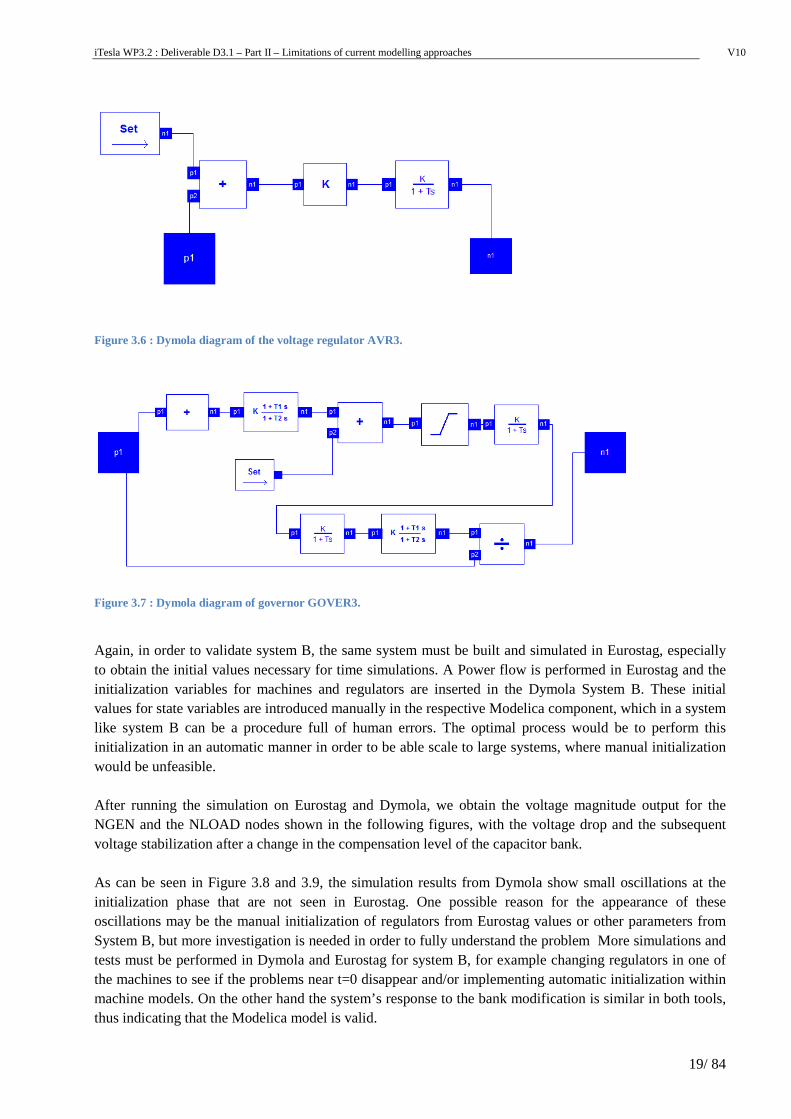
The two 1000 MW machines are fitted with a voltage regulator and a voltage governor, represented in Figure 3.6 and Figure 3.7.
iTesla WP3.2 : Deliverable D3.1 – Part II – Limitations of current modelling approaches V10
19/ 84
Figure 3.6 : Dymola diagram of the voltage regulator AVR3.
Figure 3.7 : Dymola diagram of governor GOVER3.
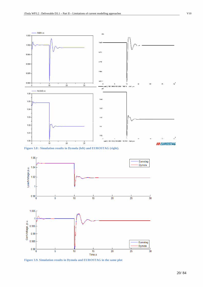
Again, in order to validate system B, the same system must be built and simulated in Eurostag, especially to obtain the initial values necessary for time simulations. A Power flow is performed in Eurostag and the initialization variables for machines and regulators are inserted in the Dymola System B. These initial values for state variables are introduced manually in the respective Modelica component, which in a system like system B can be a procedure full of human errors. The optimal process would be to perform this initialization in an automatic manner in order to be able scale to large systems, where manual initialization would be unfeasible. After running the simulation on Eurostag and Dymola, we obtain the voltage magnitude output for the NGEN and the NLOAD nodes shown in the following figures, with the voltage drop and the subsequent voltage stabilization after a change in the compensation level of the capacitor bank. As can be seen in Figure 3.8 and 3.9, the simulation results from Dymola show small oscillations at the initialization phase that are not seen in Eurostag. One possible reason for the appearance of these oscillations may be the manual initialization of regulators from Eurostag values or other parameters from System B, but more investigation is needed in order to fully understand the problem More simulations and tests must be performed in Dymola and Eurostag for system B, for example changing regulators in one of the machines to see if the problems near t=0 disappear and/or implementing automatic initialization within machine models. On the other hand the system’s response to the bank modification is similar in both tools, thus indicating that the Modelica model is valid.
iTesla WP3.2 : Deliverable D3.1 – Part II – Limitations of current modelling approaches
Figure 3.8 : Simulation results in Dymola (left) and EUROSTAG (right
Figure 3.9. Simulation results in Dymola and EUROSTAG in the same plot
Limitations of current modelling approaches
: Simulation results in Dymola (left) and EUROSTAG (right).
Figure 3.9. Simulation results in Dymola and EUROSTAG in the same plot
V10
20/ 84
iTesla WP3.2 : Deliverable D3.1 – Part II – Limitations of current modelling approaches V10
21/ 84
Another possibility would be to give initial values as guess values for Modelica solver and then run the initialization until the system reach a steady-state in Modelica solver. Then perform the time-dependent simulation starting from that initial state. In any case, the initialization problem has to be carefully investigated with the purpose of deciding the best process to follow when validating model components and systems built in Modelica.
3.1.7. Some Specific Limitations of Input/output and Equation-based Modelling
While working with phasor-based time domain power system simulation tools, such as EUROSTAG, and MODELICA, some specific limitations have been identified:
1. Limitations with shunt devices: In EUROSTAG, the voltage at the point of connection of a shunt device cannot be mathematically forced to a given value. A controller such as an AVR can be used to control the voltage. The AVR will try to keep the voltage constant, but it is not the same as mathematically imposing that the voltage on a certain node is constant. This limitation is solved using MODELICA modelling. In EUROSTAG, it is not possible to define implicit equations in the controls of a shunt element. Those limitations cannot be taken into account during the initialization process and during the integration algorithm. It is possible to define elements with implicit equations in MODELICA.
2. Limitations using multi-connector devices:
In EUROSTAG, it is possible to define correctly user-defined devices with two or more points of connection to the grid, using two or more coupled shunt devices. A drawback is that implicit functions are not correctly handled in user defined models. Explicit functions are correctly handled even in case of initialization of coupled models. MODELICA is capable to model such multi-connector devices with implicit functions.
3. Structure of the models
MODELICA should provide a more structured way to design complex devices than is currently the case. It is possible to define hierarchical links similar to object models defined in C++ code. Complex controls may also be defined through the aggregation of different simpler controls, which is also possible in many power system tools
4. Synchronization of events
In MODELICA, synchronization of events is not guaranteed. Concurrent events should be declared explicitly as such. In EUROSTAG, a similar mechanism exists.
4. AGGREGATE MODELS
4.1. Aggregate Models: Rationale
The common practice regarding modelling of large generation components has been to make use of models reproducing the performance of the individual machines with high level of accuracy and detail. With a rapidly growing amount of smaller generation units such as wind turbines and PV panels in power systems,
iTesla WP3.2 : Deliverable D3.1 – Part II – Limitations of current modelling approaches V10
22/ 84
the increased amount of input data needed to represent individual generation units as well as complexities in relation to simulation computer time especially during stability studies for large power systems is making it necessary to develop aggregated models representing a large number of individual units. For loads, aggregation is the only option, and is therefore common practice to represent distribution networks in power system studies. Due to the enormous number of loads in the power system, it is simply not possible to represent each load explicitly in the power system model. Dedicated load modelling is only feasible for a selected number of loads. This clause describes aggregation of pure wind power, PV power and load subsystems as separate tasks in the first place, and then describes how a hybrid subsystem including several or all of these components can be aggregated. The validation of the aggregation in iTesla will aim to follow the same path, validating “pure” subsystems as well as hybrid subsystems
4.2. Wind Power Aggregation
4.2.1. Methods
Several aggregation methods have been developed in relation to wind power generation modelling and have been used to represent the increasing number of wind turbines in transmission as well as distribution grids [3], [4]. These aggregation methods are based on the wind turbine models that are available in the literature or defined by the manufacturers. In order to avoid the complexity which derives from the use of manufacturer defined models, the IEC 61400-27-1 Committee Draft has specified standard dynamic electrical simulation models for wind turbines in studies of large-disturbance short term voltage stability phenomena. The proposed models should also be applicable to study other short term stability issues such as rotor angle stability, frequency stability and small-disturbance voltage stability i.e. investigating events such as short-circuits, loss of generation or loads and system separation of one synchronous area into more areas. These models are independent of any software simulation tool. Part 2 of this standard (IEC 61400-27-2) which is currently initiated will specify dynamic simulation models for the generic wind power plant topologies/configurations on the market including wind power plant control and auxiliary equipment. The work in iTesla on aggregation of wind power models will be aligned with the development of IEC 61400-27-2. Different methods of aggregation will be investigated during this process in order to define wind power plant models which will be able to simulate the response of the plant in the point of common coupling (PCC) which is considered to point of interaction between the wind power plant and the rest of the grid. The method of aggregation depends to a great extent on the type of studies as well as on the exact type of the generation technology which is included within a power plant. The common practice until today has been to assume power plants with one type of individual generation components included i.e. wind power plants with one type of wind turbines [3]. Nevertheless, there is an increased need for investigations in the near future which will address the issue of having different generation technologies within the same power plant i.e. wind turbines of different type and/or presence of PV units. Additionally, in the distribution system the aggregation of the wind turbines and PV units together with the loads should be investigated to analyse the impact of these resources to the transmission system especially for the weak grids. In this part examples from wind turbine aggregation methods are being discussed, and also the aggregation of PV technology is addressed since it is based on similar principles with the wind turbine aggregation. A decisive factor regarding wind turbine aggregation is whether the internal dynamics of the wind farm are to be studied or only the active and reactive power response at the PCC is to be simulated. In case of fixed speed wind turbines, since the speed range is very small, the usual assumption is that all wind turbines in
iTesla WP3.2 : Deliverable D3.1 – Part II – Limitations of current modelling approaches V10
23/ 84
the wind farm operate at the same speed making it possible to model the wind turbines as one single induction generator with rated power equal to the sum of the rated power of the individual wind turbines. Another crucial factor in aggregation is whether the wind speed is considered to be the same in the different wind turbine locations within the wind farm. If this is the case the drive train models can be also aggregated into one drive train with the same parameters, thus providing with the possibility to represent the wind farm by one equivalent wind turbine. However, since the size of wind farms is increasing during the last decades, the assumption of identical wind speed cannot always be applied. In this case the drive train models need to be represented explicitly. Another option is to develop aggregate models for groups of wind turbines based on the wind speed profile, making it possible to simulate wind power fluctuations more accurately. When the contribution of fixed speed wind turbines in the inertia provision during frequency events is studied the assumption of equal rotor speeds among the different wind turbines may not be sufficient. The assumption of common speed is not accurate in the case of variable speed wind turbines which operate in a large range of speeds. The common practice is to represent a wind power plant as a single wind turbine by scaling up the size of the generator and the converters, although when power fluctuations are studied this might not be enough since wind speeds can differ significantly within the large area of a wind power plant. In case of short term stability analysis, wind speed is usually considered constant and therefore simpler models can be applied. For long term stability analysis, the constant wind speed assumption may still be valid, because there is a significant smoothing of the generation if many wind turbines are aggregated into one. A very important aspect is that large wind power plants (wind farms) are normally equipped with a plant controller, which is controlling the reference values (power, reactive power / voltage) of the wind turbines are set by this wind farm controller. Therefore, it is not enough to upscale the wind turbine model, but the plant controller must also be modelled. Another issue which needs to be defined is whether and how the impedance of the wind farm cable network should be represented in those studies which require this feature. In summary, three types of aggregation method can be defined for wind turbines. The first aggregation method is the equivalencing the collector system of the wind power plant. The second aggregation method is the representation of an equivalent wind speed considering different wind speeds of each wind turbine to have a smooth generation at the PCC of the wind power plant. In this aggregation method, the representation of the mechanical system should be also investigated considering the wind turbine type. And the last aggregation method is the consideration of the overall control performance of the WPP including the wind power plant level control in addition to the wind turbine level control. Furthermore, the type of events which are investigated defines the possible aggregation methods regarding wind turbines as well as the size of the wind power plant.
4.2.2. Limitations of the wind power aggregation
In order to simulate the performance of hundreds of megawatt-size wind turbines in a transmission system, the appropriate aggregation method should be applied for the study under investigation. Inappropriate aggregated wind turbine models may cause inaccurate simulation results. Moreover, internal dynamics inside the wind power plant are not included (faults in the internal grid of the wind power plant, individual wind turbine operation and performance analysis etc). Each wind turbine connection may have different voltage dynamics, thus accuracy of reactive power and voltage control may not be implemented in the aggregated wind turbine model. For the long term dynamics wind speed fluctuations are crucial and the
iTesla WP3.2 : Deliverable D3.1 – Part II – Limitations of current modelling approaches V10
24/ 84
aggregate model might impose limitations regarding the representation of the active power dynamics. The aggregate model includes only one level of control (wind power plant controller) restricting the parameter selection options compared to the detailed models where two different control levels are included (wind turbine and wind power plant controller).
4.3. PV Power Aggregation
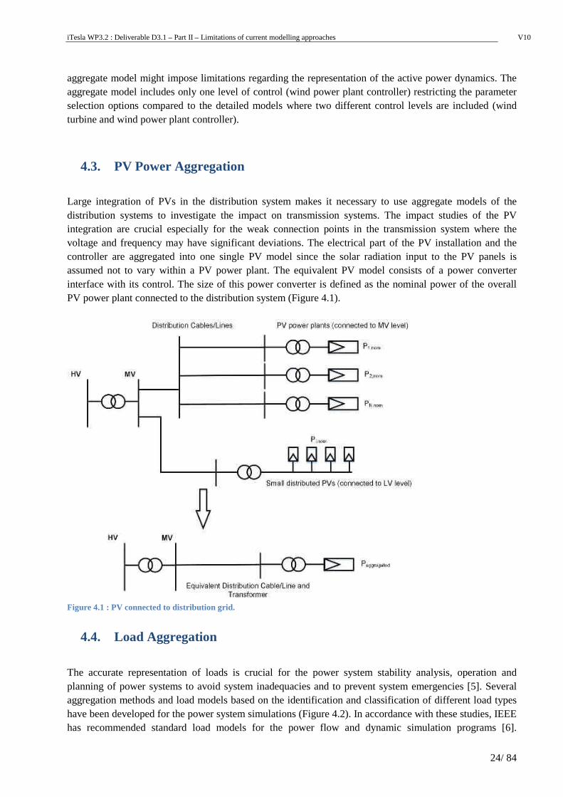
Large integration of PVs in the distribution system makes it necessary to use aggregate models of the distribution systems to investigate the impact on transmission systems. The impact studies of the PV integration are crucial especially for the weak connection points in the transmission system where the voltage and frequency may have significant deviations. The electrical part of the PV installation and the controller are aggregated into one single PV model since the solar radiation input to the PV panels is assumed not to vary within a PV power plant. The equivalent PV model consists of a power converter interface with its control. The size of this power converter is defined as the nominal power of the overall PV power plant connected to the distribution system (Figure 4.1).
Figure 4.1 : PV connected to distribution grid.
4.4. Load Aggregation
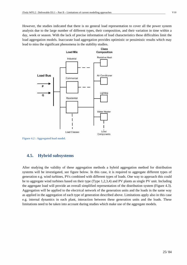
The accurate representation of loads is crucial for the power system stability analysis, operation and planning of power systems to avoid system inadequacies and to prevent system emergencies [5]. Several aggregation methods and load models based on the identification and classification of different load types have been developed for the power system simulations (Figure 4.2). In accordance with these studies, IEEE has recommended standard load models for the power flow and dynamic simulation programs [6].
iTesla WP3.2 : Deliverable D3.1 – Part II – Limitations of current modelling approaches V10
25/ 84
However, the studies indicated that there is no general load representation to cover all the power system analysis due to the large number of different types, their composition, and their variation in time within a day, week or season. With the lack of precise information of load characteristics these difficulties limit the load aggregation models. Inaccurate load aggregation provides optimistic or pessimistic results which may lead to miss the significant phenomena in the stability studies.
Figure 4.2 : Aggregated load model.
4.5. Hybrid subsystems
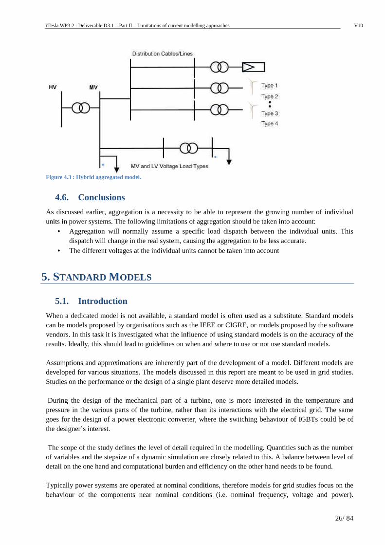
After studying the validity of these aggregation methods a hybrid aggregation method for distribution systems will be investigated, see figure below. In this case, it is required to aggregate different types of generation e.g. wind turbines, PVs combined with different types of loads. One way to approach this could be to aggregate wind turbines based on their type (Type 1,2,3,4) and PV plants as single PV unit. Including the aggregate load will provide an overall simplified representation of the distribution system (Figure 4.3). Aggregation will be applied to the electrical network of the generation units and the loads in the same way as applied in the aggregation of each type of generation described above. Limitations apply also in this case e.g. internal dynamics in each plant, interaction between these generation units and the loads. These limitations need to be taken into account during studies which make use of the aggregate models.
iTesla WP3.2 : Deliverable D3.1 – Part II – Limitations of current modelling approaches V10
26/ 84
Figure 4.3 : Hybrid aggregated model.
4.6. Conclusions
As discussed earlier, aggregation is a necessity to be able to represent the growing number of individual units in power systems. The following limitations of aggregation should be taken into account:
• Aggregation will normally assume a specific load dispatch between the individual units. This dispatch will change in the real system, causing the aggregation to be less accurate.
• The different voltages at the individual units cannot be taken into account
5. STANDARD MODELS
5.1. Introduction
When a dedicated model is not available, a standard model is often used as a substitute. Standard models can be models proposed by organisations such as the IEEE or CIGRE, or models proposed by the software vendors. In this task it is investigated what the influence of using standard models is on the accuracy of the results. Ideally, this should lead to guidelines on when and where to use or not use standard models. Assumptions and approximations are inherently part of the development of a model. Different models are developed for various situations. The models discussed in this report are meant to be used in grid studies. Studies on the performance or the design of a single plant deserve more detailed models. During the design of the mechanical part of a turbine, one is more interested in the temperature and pressure in the various parts of the turbine, rather than its interactions with the electrical grid. The same goes for the design of a power electronic converter, where the switching behaviour of IGBTs could be of the designer’s interest. The scope of the study defines the level of detail required in the modelling. Quantities such as the number of variables and the stepsize of a dynamic simulation are closely related to this. A balance between level of detail on the one hand and computational burden and efficiency on the other hand needs to be found. Typically power systems are operated at nominal conditions, therefore models for grid studies focus on the behaviour of the components near nominal conditions (i.e. nominal frequency, voltage and power).
iTesla WP3.2 : Deliverable D3.1 – Part II – Limitations of current modelling approaches V10
27/ 84
Moreover, in grid studies thousands of controllers for generating units and protection devices may have to be implemented in the same model. However, over the years, certain models are accepted as standard. Often they are used without much precaution, as in many studies and literature these “standard” models are used as a passkey. The next section gives an overview of wind turbine models and demonstrates the differences between various standard models for gas turbines. An overview of the frequently used standard models is given. Next the main functionalities of the model are discussed. We conclude with a thorough discussion on the approximations and assumptions made in the different models. By acknowledging these approximations and assumptions, an appreciation of the accuracy can be given for different operating conditions.
5.2. Standard electrical models for wind power generation
The wind turbine models presented in this section have been proposed by the IEC Technical Committee 88 Working Group 27 (TC88 WG27) in the ongoing work of the standard IEC 61400-27 for “Electrical simulation models for wind power generation”. The purpose of this standardization work is to define generic simulation models for wind turbines (part 1) and wind power plants (part 2), which are intended for short-term power system stability analyses. The Committee Draft, which was submitted in January 2012, describes generic wind turbine models and a procedure for validation of wind turbine models. The generic model description includes a general model structure covering existing as well as future types of wind turbines, and specific fundamental frequency positive sequence models for the four wind turbine types which are widely used today. The validation procedure can be applied to the generic models specified in the standard, or to manufacturer specific fundamental frequency models.
5.2.1. Model specifications
The following specifications apply to the proposed models: • Model(s) should be developed to span at least the existing four categories of currently developed wind turbine generator technologies: conventional asynchronous generators (Type 1), variable rotor resistance asynchronous generators (Type 2), doubly-fed asynchronous generators (Type 3) and full-converter interface units (Type 4). • The models should be modular in nature to allow for the potential of augmentation in case of other wind turbine types including future technologies being developed, or future supplemental controls features. • The models are to be used primarily for short term power system stability studies and thus should represent all dynamics affected and relevant during
• short circuits (balanced and unbalanced1) on the transmission grid (external to the wind power plant, including voltage recovery), • grid frequency disturbances, • electromechanical modes of synchronous generator rotor oscillations (typically in the 0.2 to 4 Hz range), and • reference value changes.
• The models are for fundamental frequency positive sequence response. • The models should be valid for typical power system frequency deviations (recommended +/- 6% from system nominal frequency). • The models should be able to handle numerically the simulation of phase jumps. • The models should be valid for steady state voltage deviations (recommended +/- 10% from system nominal voltage). In addition, they should be valid for dynamic voltage phenomena (e.g. faults) where the voltage can drop temporarily to zero.
iTesla WP3.2 : Deliverable D3.1 – Part II – Limitations of current modelling approaches V10
28/ 84
• The typical simulation time frame of interest is from 10 to 30 seconds. Wind speed is assumed to be constant during such a time frame. • The models should work with integration time steps up to ¼ cycle. As a consequence, the bandwidth of the models cannot be greater than 15 Hz. Also, the bandwidth of the models is not intended to be greater than 15 Hz and so all higher frequency dynamics are neglected. • The models should initialize to a steady state from power flow solutions at full or partial power. • External conditions like initial wind speed should be taken into account where they can have significant influence on the power swings. • Over/under frequency and over/under voltage protection should be modelled. These may be implemented in separate supplemental modules that connect to the main wind turbine generator model. • The turbine-generator inertia and first shaft torsional mode should be taken into account where it can have significant influence on the power swings. • The models should be numerically sound so that they can be applied in both high and low short circuit systems. The equipment suppliers shall establish the minimum short circuit ratio and/or system conditions for which the model is applicable for their specific equipment. Dynamics of phase-locked loops are not included in the models. • The models should be clearly specified with block diagrams, explanation of non-linear components and equations in the models, and discussion of any unique initialization issues to allow for any software vendor to implement the models. The standard will not describe the algorithms that are applied in the specific time series simulation tools, but only the linear, non-linear and differential relations that are modelled. • The generic wind turbine models will include generic models for protection and control systems, which will inevitably deviate from specific manufacturer systems. The models should easily be parameterized to represent any manufacturer specific systems, which will be done by definition of distinct blocks for protection and control. This structure will make it possible to replace the generic control and protection system blocks with manufacturer specific blocks. • The model should include the reactive power capability of the wind turbine. Limitations which apply to these model descriptions are:
• The models are not intended for long term stability analysis.
• The models are not intended for investigation of sub-synchronous interaction phenomena • The models are not intended for investigation of the fluctuations originating from wind speed
variability in time and space. This implies that the models are not including phenomena such as turbulence, tower shadow, wind shear and wakes. The models do not cover phenomena such as harmonics, flicker or any other EMC emissions included in the IEC 61000 series.
• The models have not been developed explicitly with eigenvalue calculation (for small signal stability) in mind.
• The models specified here apply only to wind turbines, and therefore do not include wind power plant level controls and additional equipment such as SVCs, STATCOMs and other devices which will be covered by part 2.
• This standard does not address the specifics of short circuit calculations • The models are not applicable to studies of extremely weak systems including situations where
wind turbines are islanded without synchronous generation.
5.2.2. Wind turbine, plant and grid model interfaces
The General dynamic simulation interface between wind turbine model and grid model is illustrated in the following figure. The model can either be excited by an event in the grid model such as a short-circuit, or by a change in a wind turbine reference value from the plant controller.
iTesla WP3.2 : Deliverable D3.1 – Part II – Limitations of current modelling approaches V10
29/ 84
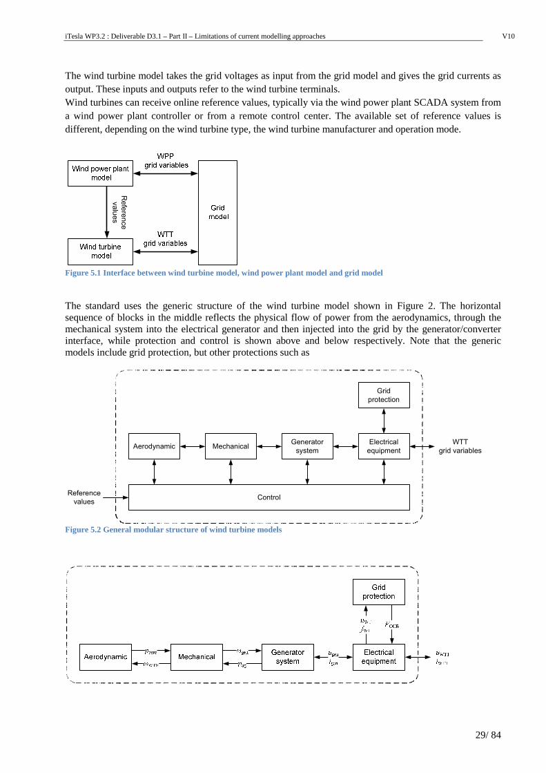
The wind turbine model takes the grid voltages as input from the grid model and gives the grid currents as output. These inputs and outputs refer to the wind turbine terminals. Wind turbines can receive online reference values, typically via the wind power plant SCADA system from a wind power plant controller or from a remote control center. The available set of reference values is different, depending on the wind turbine type, the wind turbine manufacturer and operation mode.
Figure 5.1 Interface between wind turbine model, wind power plant model and grid model
The standard uses the generic structure of the wind turbine model shown in Figure 2. The horizontal sequence of blocks in the middle reflects the physical flow of power from the aerodynamics, through the mechanical system into the electrical generator and then injected into the grid by the generator/converter interface, while protection and control is shown above and below respectively. Note that the generic models include grid protection, but other protections such as
Figure 5.2 General modular structure of wind turbine models
Refe
rence
valu
es
Aerodynamic Mechanical Electrical
equipment
Control
Grid
protection
Generator
system
Reference
values
WTT
grid variables
iTesla WP3.2 : Deliverable D3.1 – Part II – Limitations of current modelling approaches V10
30/ 84
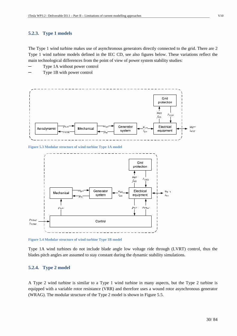
5.2.3. Type 1 models
The Type 1 wind turbine makes use of asynchronous generators directly connected to the grid. There are 2 Type 1 wind turbine models defined in the IEC CD, see also figures below. These variations reflect the main technological differences from the point of view of power system stability studies: ─ Type 1A without power control ─ Type 1B with power control
Figure 5.3 Modular structure of wind turbine Type 1A model
Figure 5.4 Modular structure of wind turbine Type 1B model
Type 1A wind turbines do not include blade angle low voltage ride through (LVRT) control, thus the blades pitch angles are assumed to stay constant during the dynamic stability simulations.
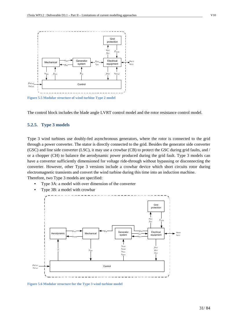
5.2.4. Type 2 model
A Type 2 wind turbine is similar to a Type 1 wind turbine in many aspects, but the Type 2 turbine is equipped with a variable rotor resistance (VRR) and therefore uses a wound rotor asynchronous generator (WRAG). The modular structure of the Type 2 model is shown in Figure 5.5.
iTesla WP3.2 : Deliverable D3.1 – Part II – Limitations of current modelling approaches V10
31/ 84
Figure 5.5 Modular structure of wind turbine Type 2 model
The control block includes the blade angle LVRT control model and the rotor resistance control model.
5.2.5. Type 3 models
Type 3 wind turbines use doubly-fed asynchronous generators, where the rotor is connected to the grid through a power converter. The stator is directly connected to the grid. Besides the generator side converter (GSC) and line side converter (LSC), it may use a crowbar (CB) to protect the GSC during grid faults, and / or a chopper (CH) to balance the aerodynamic power produced during the grid fault. Type 3 models can have a converter sufficiently dimensioned for voltage ride-through without bypassing or disconnecting the converter. However, other Type 3 versions include a crowbar device which short circuits rotor during electromagnetic transients and convert the wind turbine during this time into an induction machine. Therefore, two Type 3 models are specified:
• Type 3A: a model with over dimension of the converter • Type 3B: a model with crowbar
Aerodynamic MechanicalElectrical
equipment
Grid
protection
paeroiWT
FOCB
Control
θ
pWTqWTuWT
iPcmdiQcmdiPmaxiQmax
ωWTR
ωgen
uWTfWT
pWTpag Generator
systemuWT
pWTrefxWTref
uWTTiWTT
Figure 5.6 Modular structure for the Type 3 wind turbine model
MechanicalGenerator
systempag
ωgen
Control
paeroωgen
ugenigen
Rrot
Electrical
equipment
Grid
protection
FOCBuWTfWT
pWTrefxWTref
uWTTiWTT
pWT xWTref
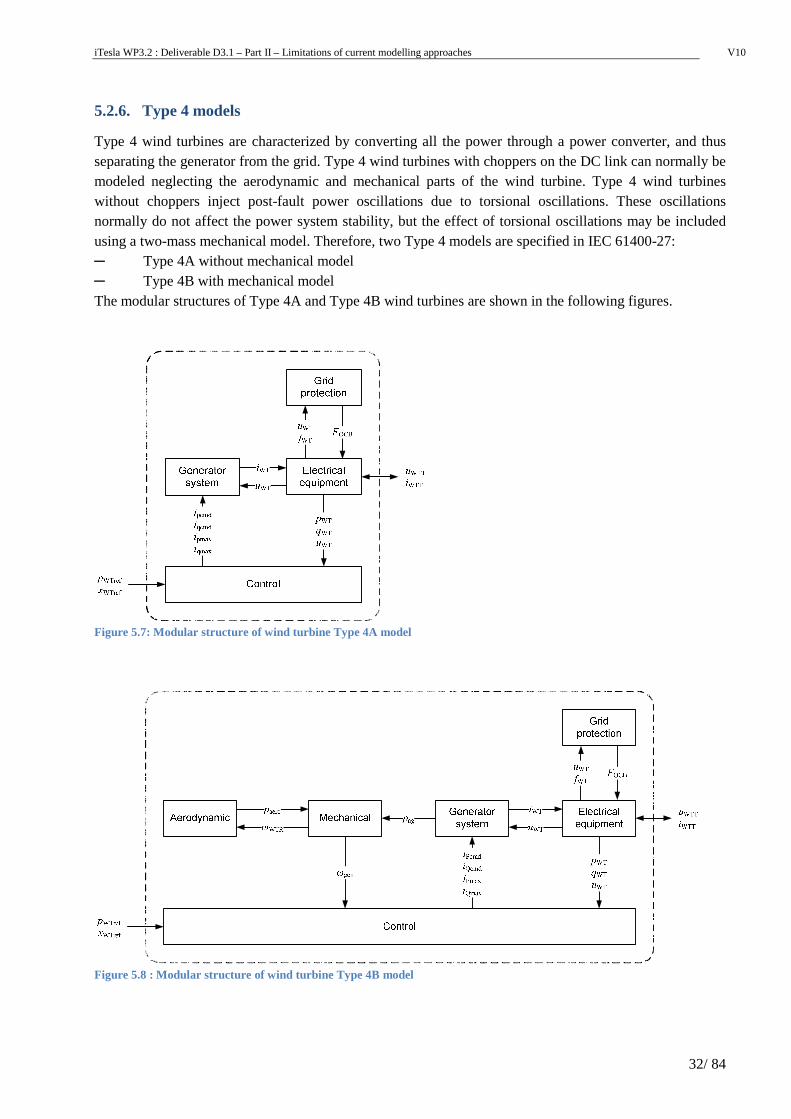
iTesla WP3.2 : Deliverable D3.1 – Part II – Limitations of current modelling approaches V10
32/ 84
5.2.6. Type 4 models
Type 4 wind turbines are characterized by converting all the power through a power converter, and thus separating the generator from the grid. Type 4 wind turbines with choppers on the DC link can normally be modeled neglecting the aerodynamic and mechanical parts of the wind turbine. Type 4 wind turbines without choppers inject post-fault power oscillations due to torsional oscillations. These oscillations normally do not affect the power system stability, but the effect of torsional oscillations may be included using a two-mass mechanical model. Therefore, two Type 4 models are specified in IEC 61400-27: ─ Type 4A without mechanical model ─ Type 4B with mechanical model The modular structures of Type 4A and Type 4B wind turbines are shown in the following figures.
Figure 5.7: Modular structure of wind turbine Type 4A model
Figure 5.8 : Modular structure of wind turbine Type 4B model
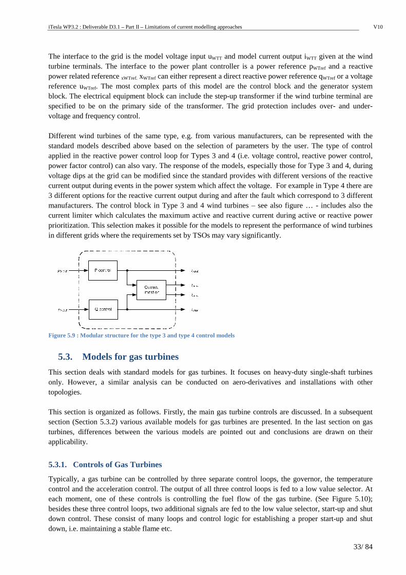
iTesla WP3.2 : Deliverable D3.1 – Part II – Limitations of current modelling approaches V10
33/ 84
The interface to the grid is the model voltage input uWTT and model current output iWTT given at the wind turbine terminals. The interface to the power plant controller is a power reference pWTref and a reactive power related reference xWTref. xWTref can either represent a direct reactive power reference qWTref or a voltage reference uWTref. The most complex parts of this model are the control block and the generator system block. The electrical equipment block can include the step-up transformer if the wind turbine terminal are specified to be on the primary side of the transformer. The grid protection includes over- and under- voltage and frequency control. Different wind turbines of the same type, e.g. from various manufacturers, can be represented with the standard models described above based on the selection of parameters by the user. The type of control applied in the reactive power control loop for Types 3 and 4 (i.e. voltage control, reactive power control, power factor control) can also vary. The response of the models, especially those for Type 3 and 4, during voltage dips at the grid can be modified since the standard provides with different versions of the reactive current output during events in the power system which affect the voltage. For example in Type 4 there are 3 different options for the reactive current output during and after the fault which correspond to 3 different manufacturers. The control block in Type 3 and 4 wind turbines – see also figure … - includes also the current limiter which calculates the maximum active and reactive current during active or reactive power prioritization. This selection makes it possible for the models to represent the performance of wind turbines in different grids where the requirements set by TSOs may vary significantly.
Figure 5.9 : Modular structure for the type 3 and type 4 control models
5.3. Models for gas turbines
This section deals with standard models for gas turbines. It focuses on heavy-duty single-shaft turbines only. However, a similar analysis can be conducted on aero-derivatives and installations with other topologies. This section is organized as follows. Firstly, the main gas turbine controls are discussed. In a subsequent section (Section 5.3.2) various available models for gas turbines are presented. In the last section on gas turbines, differences between the various models are pointed out and conclusions are drawn on their applicability.
5.3.1. Controls of Gas Turbines
Typically, a gas turbine can be controlled by three separate control loops, the governor, the temperature control and the acceleration control. The output of all three control loops is fed to a low value selector. At each moment, one of these controls is controlling the fuel flow of the gas turbine. (See Figure 5.10); besides these three control loops, two additional signals are fed to the low value selector, start-up and shut down control. These consist of many loops and control logic for establishing a proper start-up and shut down, i.e. maintaining a stable flame etc.
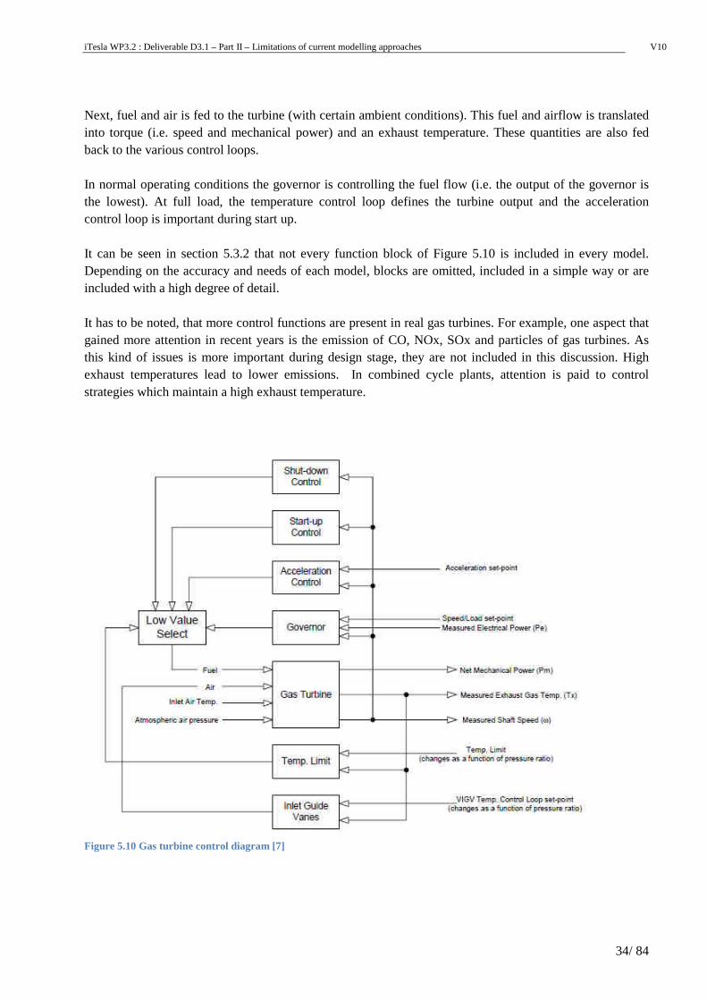
iTesla WP3.2 : Deliverable D3.1 – Part II – Limitations of current modelling approaches V10
34/ 84
Next, fuel and air is fed to the turbine (with certain ambient conditions). This fuel and airflow is translated into torque (i.e. speed and mechanical power) and an exhaust temperature. These quantities are also fed back to the various control loops. In normal operating conditions the governor is controlling the fuel flow (i.e. the output of the governor is the lowest). At full load, the temperature control loop defines the turbine output and the acceleration control loop is important during start up. It can be seen in section 5.3.2 that not every function block of Figure 5.10 is included in every model. Depending on the accuracy and needs of each model, blocks are omitted, included in a simple way or are included with a high degree of detail. It has to be noted, that more control functions are present in real gas turbines. For example, one aspect that gained more attention in recent years is the emission of CO, NOx, SOx and particles of gas turbines. As this kind of issues is more important during design stage, they are not included in this discussion. High exhaust temperatures lead to lower emissions. In combined cycle plants, attention is paid to control strategies which maintain a high exhaust temperature.
Figure 5.10 Gas turbine control diagram [7]
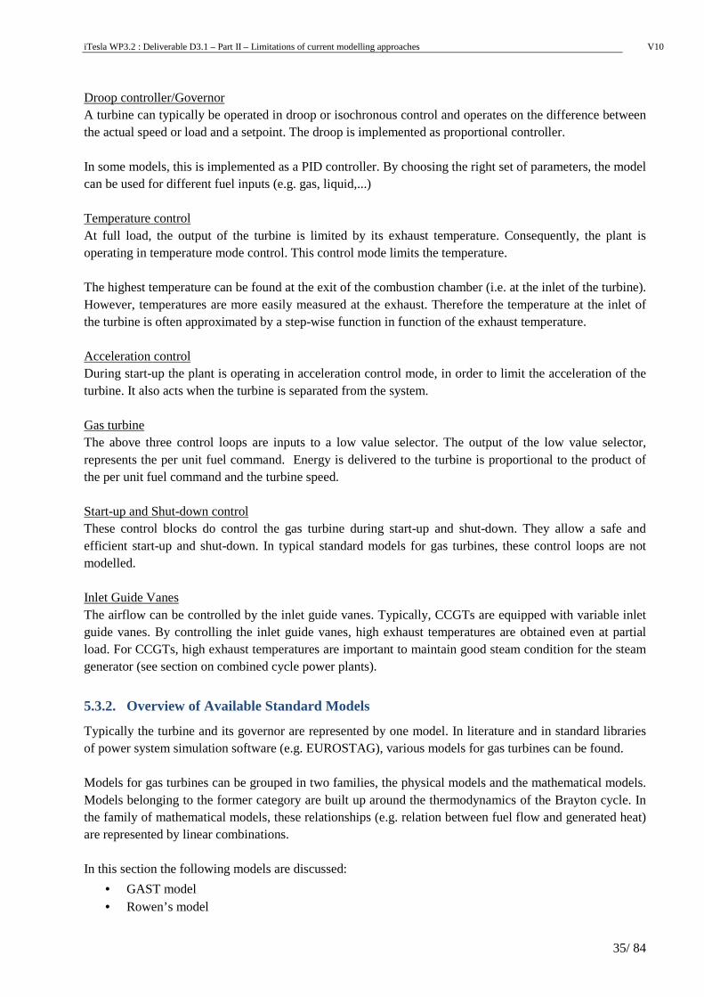
iTesla WP3.2 : Deliverable D3.1 – Part II – Limitations of current modelling approaches V10
35/ 84
Droop controller/Governor A turbine can typically be operated in droop or isochronous control and operates on the difference between the actual speed or load and a setpoint. The droop is implemented as proportional controller. In some models, this is implemented as a PID controller. By choosing the right set of parameters, the model can be used for different fuel inputs (e.g. gas, liquid,...) Temperature control At full load, the output of the turbine is limited by its exhaust temperature. Consequently, the plant is operating in temperature mode control. This control mode limits the temperature. The highest temperature can be found at the exit of the combustion chamber (i.e. at the inlet of the turbine). However, temperatures are more easily measured at the exhaust. Therefore the temperature at the inlet of the turbine is often approximated by a step-wise function in function of the exhaust temperature. Acceleration control During start-up the plant is operating in acceleration control mode, in order to limit the acceleration of the turbine. It also acts when the turbine is separated from the system. Gas turbine The above three control loops are inputs to a low value selector. The output of the low value selector, represents the per unit fuel command. Energy is delivered to the turbine is proportional to the product of the per unit fuel command and the turbine speed. Start-up and Shut-down control These control blocks do control the gas turbine during start-up and shut-down. They allow a safe and efficient start-up and shut-down. In typical standard models for gas turbines, these control loops are not modelled. Inlet Guide Vanes The airflow can be controlled by the inlet guide vanes. Typically, CCGTs are equipped with variable inlet guide vanes. By controlling the inlet guide vanes, high exhaust temperatures are obtained even at partial load. For CCGTs, high exhaust temperatures are important to maintain good steam condition for the steam generator (see section on combined cycle power plants).
5.3.2. Overview of Available Standard Models
Typically the turbine and its governor are represented by one model. In literature and in standard libraries of power system simulation software (e.g. EUROSTAG), various models for gas turbines can be found. Models for gas turbines can be grouped in two families, the physical models and the mathematical models. Models belonging to the former category are built up around the thermodynamics of the Brayton cycle. In the family of mathematical models, these relationships (e.g. relation between fuel flow and generated heat) are represented by linear combinations. In this section the following models are discussed:
• GAST model • Rowen’s model
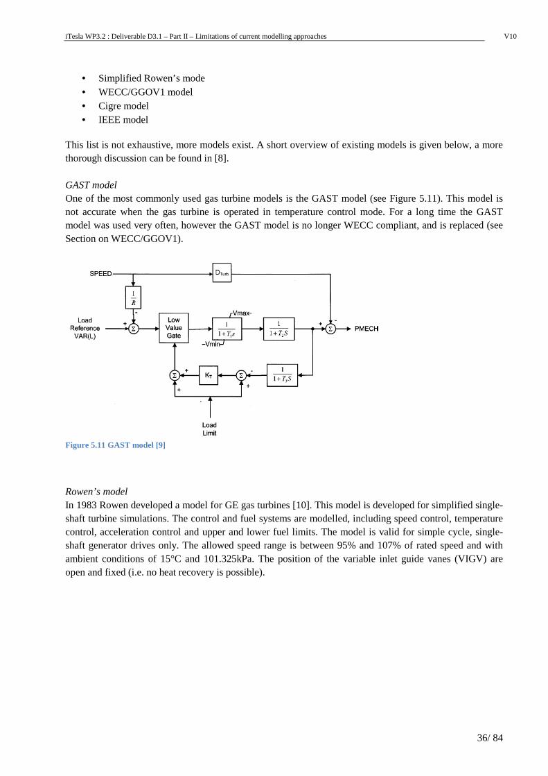
iTesla WP3.2 : Deliverable D3.1 – Part II – Limitations of current modelling approaches V10
36/ 84
• Simplified Rowen’s mode • WECC/GGOV1 model • Cigre model • IEEE model
This list is not exhaustive, more models exist. A short overview of existing models is given below, a more thorough discussion can be found in [8]. GAST model One of the most commonly used gas turbine models is the GAST model (see Figure 5.11). This model is not accurate when the gas turbine is operated in temperature control mode. For a long time the GAST model was used very often, however the GAST model is no longer WECC compliant, and is replaced (see Section on WECC/GGOV1).
Figure 5.11 GAST model [9]
Rowen’s model In 1983 Rowen developed a model for GE gas turbines [10]. This model is developed for simplified single-shaft turbine simulations. The control and fuel systems are modelled, including speed control, temperature control, acceleration control and upper and lower fuel limits. The model is valid for simple cycle, single-shaft generator drives only. The allowed speed range is between 95% and 107% of rated speed and with ambient conditions of 15°C and 101.325kPa. The position of the variable inlet guide vanes (VIGV) are open and fixed (i.e. no heat recovery is possible).
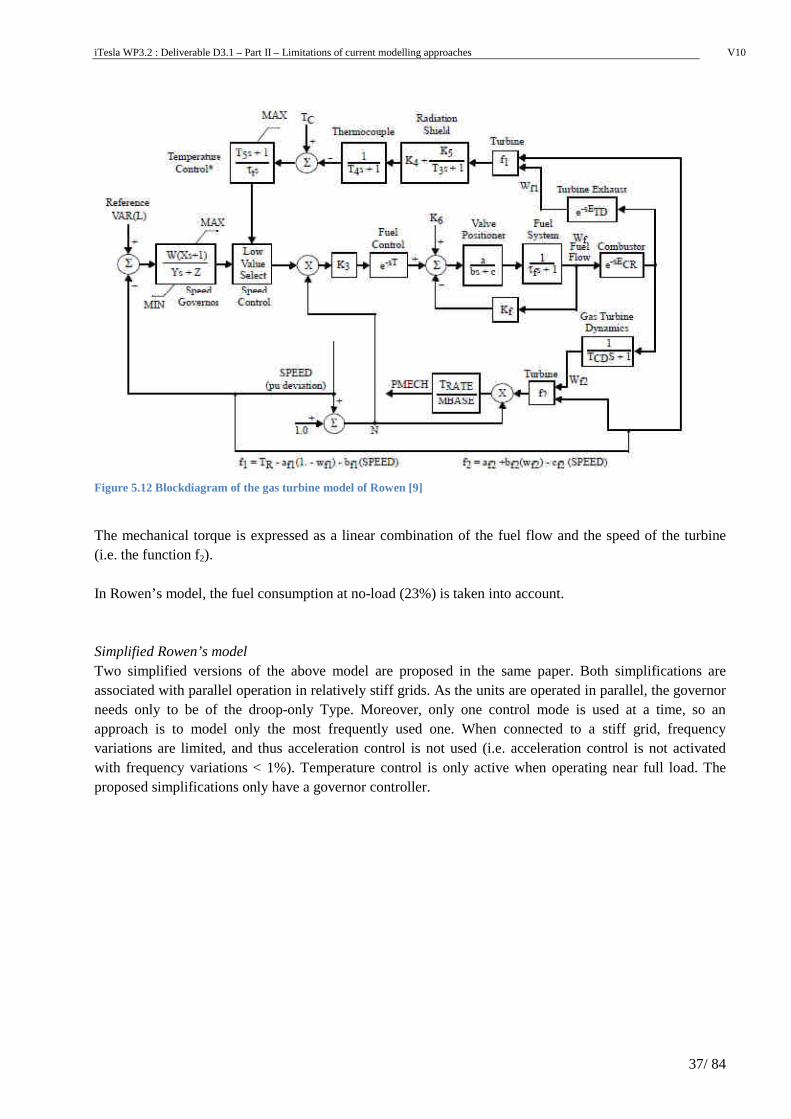
iTesla WP3.2 : Deliverable D3.1 – Part II – Limitations of current modelling approaches V10
37/ 84
Figure 5.12 Blockdiagram of the gas turbine model of Rowen [9]
The mechanical torque is expressed as a linear combination of the fuel flow and the speed of the turbine (i.e. the function f2). In Rowen’s model, the fuel consumption at no-load (23%) is taken into account. Simplified Rowen’s model Two simplified versions of the above model are proposed in the same paper. Both simplifications are associated with parallel operation in relatively stiff grids. As the units are operated in parallel, the governor needs only to be of the droop-only Type. Moreover, only one control mode is used at a time, so an approach is to model only the most frequently used one. When connected to a stiff grid, frequency variations are limited, and thus acceleration control is not used (i.e. acceleration control is not activated with frequency variations < 1%). Temperature control is only active when operating near full load. The proposed simplifications only have a governor controller.
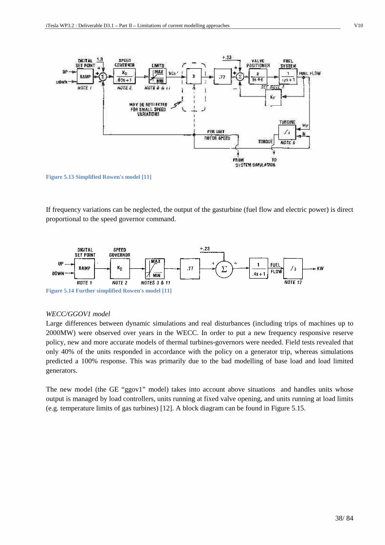
iTesla WP3.2 : Deliverable D3.1 – Part II – Limitations of current modelling approaches V10
38/ 84
Figure 5.13 Simplified Rowen's model [11]
If frequency variations can be neglected, the output of the gasturbine (fuel flow and electric power) is direct proportional to the speed governor command.
Figure 5.14 Further simplified Rowen's model [11]
WECC/GGOV1 model Large differences between dynamic simulations and real disturbances (including trips of machines up to 2000MW) were observed over years in the WECC. In order to put a new frequency responsive reserve policy, new and more accurate models of thermal turbines-governors were needed. Field tests revealed that only 40% of the units responded in accordance with the policy on a generator trip, whereas simulations predicted a 100% response. This was primarily due to the bad modelling of base load and load limited generators. The new model (the GE “ggov1” model) takes into account above situations and handles units whose output is managed by load controllers, units running at fixed valve opening, and units running at load limits (e.g. temperature limits of gas turbines) [12]. A block diagram can be found in Figure 5.15.
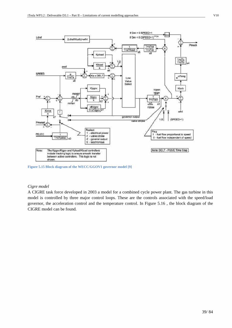
iTesla WP3.2 : Deliverable D3.1 – Part II – Limitations of current modelling approaches V10
39/ 84
Figure 5.15 Block diagram of the WECC/GGOV1 governor model [9]
Cigre model A CIGRE task force developed in 2003 a model for a combined cycle power plant. The gas turbine in this model is controlled by three major control loops. These are the controls associated with the speed/load governor, the acceleration control and the temperature control. In Figure 5.16 , the block diagram of the CIGRE model can be found.
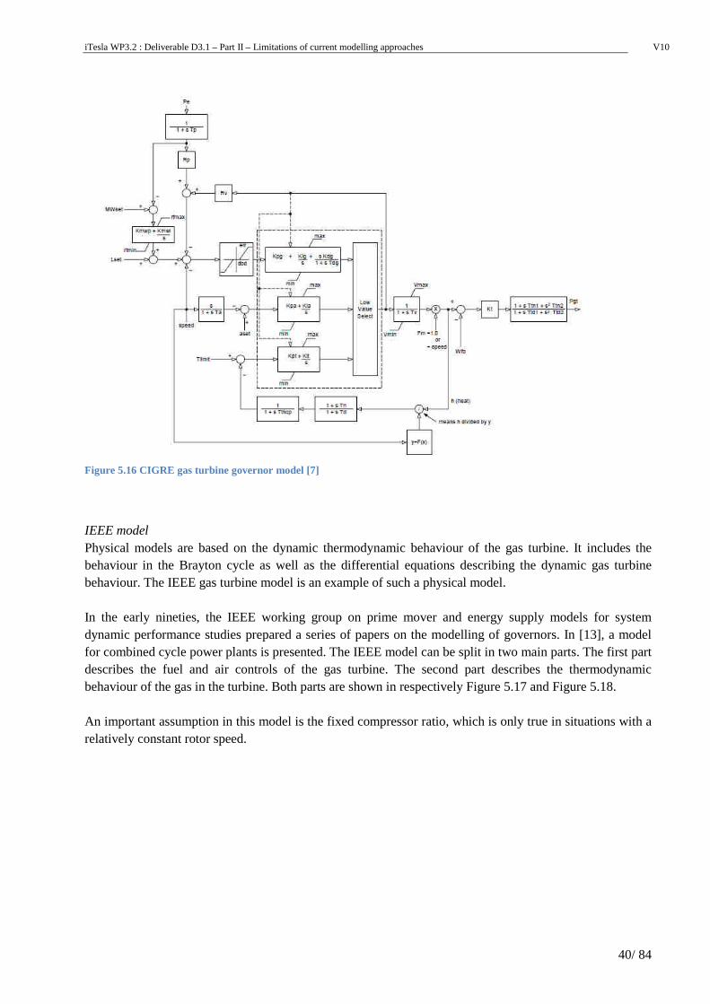
iTesla WP3.2 : Deliverable D3.1 – Part II – Limitations of current modelling approaches V10
40/ 84
Figure 5.16 CIGRE gas turbine governor model [7]
IEEE model Physical models are based on the dynamic thermodynamic behaviour of the gas turbine. It includes the behaviour in the Brayton cycle as well as the differential equations describing the dynamic gas turbine behaviour. The IEEE gas turbine model is an example of such a physical model. In the early nineties, the IEEE working group on prime mover and energy supply models for system dynamic performance studies prepared a series of papers on the modelling of governors. In [13], a model for combined cycle power plants is presented. The IEEE model can be split in two main parts. The first part describes the fuel and air controls of the gas turbine. The second part describes the thermodynamic behaviour of the gas in the turbine. Both parts are shown in respectively Figure 5.17 and Figure 5.18. An important assumption in this model is the fixed compressor ratio, which is only true in situations with a relatively constant rotor speed.
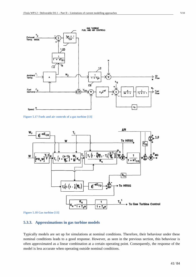
iTesla WP3.2 : Deliverable D3.1 – Part II – Limitations of current modelling approaches V10
41/ 84
Figure 5.17 Fuels and air controls of a gas turbine [13]
Figure 5.18 Gas turbine [13]
5.3.3. Approximations in gas turbine models
Typically models are set up for simulations at nominal conditions. Therefore, their behaviour under these nominal conditions leads to a good response. However, as seen in the previous section, this behaviour is often approximated as a linear combination at a certain operating point. Consequently, the response of the model is less accurate when operating outside nominal conditions.
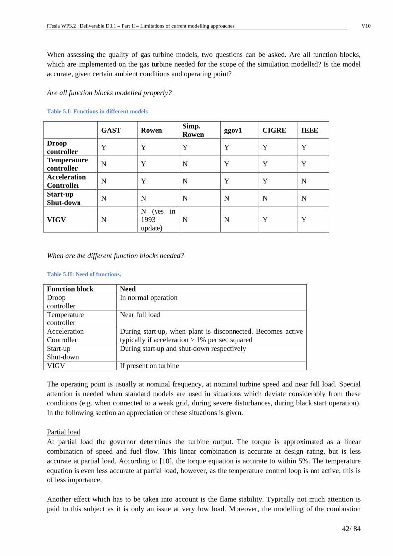
iTesla WP3.2 : Deliverable D3.1 – Part II – Limitations of current modelling approaches V10
42/ 84
When assessing the quality of gas turbine models, two questions can be asked. Are all function blocks, which are implemented on the gas turbine needed for the scope of the simulation modelled? Is the model accurate, given certain ambient conditions and operating point? Are all function blocks modelled properly? Table 5.I: Functions in different models
GAST Rowen Simp. Rowen ggov1 CIGRE IEEE
Droop controller
Y Y Y Y Y Y
Temperature controller
N Y N Y Y Y
Acceleration Controller
N Y N Y Y N
Start-up Shut-down
N N N N N N
VIGV N N (yes in 1993 update)
N N Y Y
When are the different function blocks needed? Table 5.II: Need of functions.
Function block Need Droop controller
In normal operation
Temperature controller
Near full load
Acceleration Controller
During start-up, when plant is disconnected. Becomes active typically if acceleration > 1% per sec squared
Start-up Shut-down
During start-up and shut-down respectively
VIGV If present on turbine The operating point is usually at nominal frequency, at nominal turbine speed and near full load. Special attention is needed when standard models are used in situations which deviate considerably from these conditions (e.g. when connected to a weak grid, during severe disturbances, during black start operation). In the following section an appreciation of these situations is given. Partial load At partial load the governor determines the turbine output. The torque is approximated as a linear combination of speed and fuel flow. This linear combination is accurate at design rating, but is less accurate at partial load. According to [10], the torque equation is accurate to within 5%. The temperature equation is even less accurate at partial load, however, as the temperature control loop is not active; this is of less importance. Another effect which has to be taken into account is the flame stability. Typically not much attention is paid to this subject as it is only an issue at very low load. Moreover, the modelling of the combustion
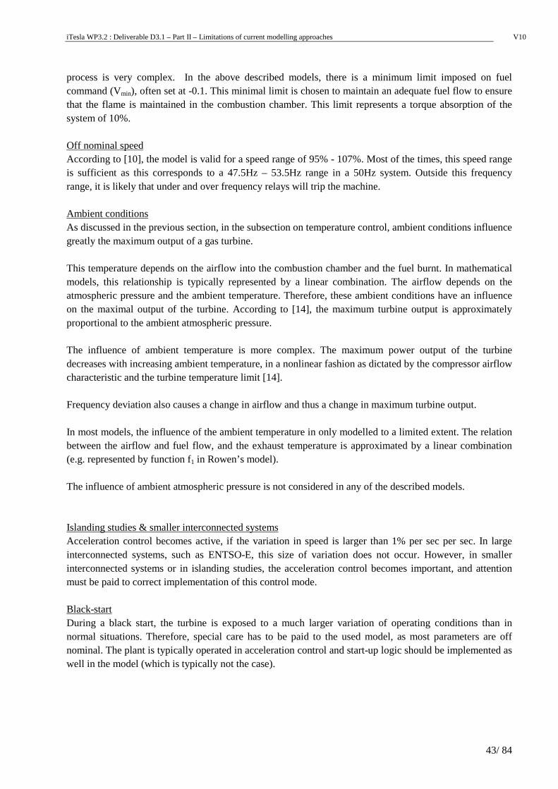
iTesla WP3.2 : Deliverable D3.1 – Part II – Limitations of current modelling approaches V10
43/ 84
process is very complex. In the above described models, there is a minimum limit imposed on fuel command (Vmin), often set at -0.1. This minimal limit is chosen to maintain an adequate fuel flow to ensure that the flame is maintained in the combustion chamber. This limit represents a torque absorption of the system of 10%. Off nominal speed According to [10], the model is valid for a speed range of 95% - 107%. Most of the times, this speed range is sufficient as this corresponds to a 47.5Hz – 53.5Hz range in a 50Hz system. Outside this frequency range, it is likely that under and over frequency relays will trip the machine. Ambient conditions As discussed in the previous section, in the subsection on temperature control, ambient conditions influence greatly the maximum output of a gas turbine. This temperature depends on the airflow into the combustion chamber and the fuel burnt. In mathematical models, this relationship is typically represented by a linear combination. The airflow depends on the atmospheric pressure and the ambient temperature. Therefore, these ambient conditions have an influence on the maximal output of the turbine. According to [14], the maximum turbine output is approximately proportional to the ambient atmospheric pressure. The influence of ambient temperature is more complex. The maximum power output of the turbine decreases with increasing ambient temperature, in a nonlinear fashion as dictated by the compressor airflow characteristic and the turbine temperature limit [14]. Frequency deviation also causes a change in airflow and thus a change in maximum turbine output. In most models, the influence of the ambient temperature in only modelled to a limited extent. The relation between the airflow and fuel flow, and the exhaust temperature is approximated by a linear combination (e.g. represented by function f1 in Rowen’s model). The influence of ambient atmospheric pressure is not considered in any of the described models. Islanding studies & smaller interconnected systems Acceleration control becomes active, if the variation in speed is larger than 1% per sec per sec. In large interconnected systems, such as ENTSO-E, this size of variation does not occur. However, in smaller interconnected systems or in islanding studies, the acceleration control becomes important, and attention must be paid to correct implementation of this control mode. Black-start During a black start, the turbine is exposed to a much larger variation of operating conditions than in normal situations. Therefore, special care has to be paid to the used model, as most parameters are off nominal. The plant is typically operated in acceleration control and start-up logic should be implemented as well in the model (which is typically not the case).
iTesla WP3.2 : Deliverable D3.1 – Part II – Limitations of current modelling approaches V10
44/ 84
5.3.4. The ALSTOM GT26 Model
In the CIGRE brochure [15], a detailed description of Alstom gas turbines is provided by Alstom. As an example of a model for a specific type of turbine (in contrast with generic models), this model is discussed here and compared with generic models. Alstom states that this dynamic model is a simplified version. Many functions are not of interest in power system dynamic studies, such as start-up, process protection. Hence this model is not suited for certain scenarios.
The main block of the model consists of the governor. A frequency error signal is passed via a deadband (static or enhanced dynamic) to a gain that converts this signal into a power demand signal. Next, modules are present in order to represent the physical constraints (power limitations module), physics of the air and fuel flow (power distribution module) and turbine dynamics (GT dynamics module), see Figure 5.19. More information on the different modules can be found in [15].
5.3.5. Comparison of the ALSTOM GT26 Model with Standard Models
As an example of the performance of various models for gas turbines (both generic and specific ones), the following example is constructed.
Figure 5.19 Configuration of the Alstom gas turbine-governor system [15]
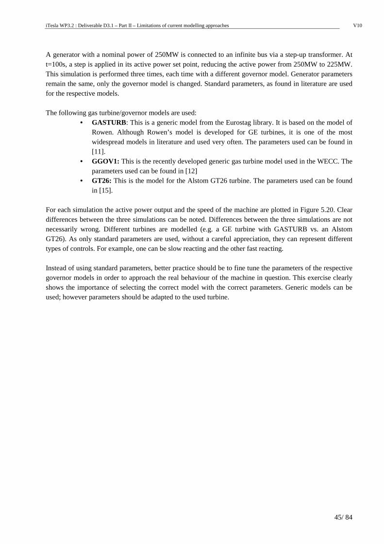
iTesla WP3.2 : Deliverable D3.1 – Part II – Limitations of current modelling approaches V10
45/ 84
A generator with a nominal power of 250MW is connected to an infinite bus via a step-up transformer. At t=100s, a step is applied in its active power set point, reducing the active power from 250MW to 225MW. This simulation is performed three times, each time with a different governor model. Generator parameters remain the same, only the governor model is changed. Standard parameters, as found in literature are used for the respective models. The following gas turbine/governor models are used:
• GASTURB: This is a generic model from the Eurostag library. It is based on the model of Rowen. Although Rowen’s model is developed for GE turbines, it is one of the most widespread models in literature and used very often. The parameters used can be found in [11].
• GGOV1: This is the recently developed generic gas turbine model used in the WECC. The parameters used can be found in [12]
• GT26: This is the model for the Alstom GT26 turbine. The parameters used can be found in [15].
For each simulation the active power output and the speed of the machine are plotted in Figure 5.20. Clear differences between the three simulations can be noted. Differences between the three simulations are not necessarily wrong. Different turbines are modelled (e.g. a GE turbine with GASTURB vs. an Alstom GT26). As only standard parameters are used, without a careful appreciation, they can represent different types of controls. For example, one can be slow reacting and the other fast reacting. Instead of using standard parameters, better practice should be to fine tune the parameters of the respective governor models in order to approach the real behaviour of the machine in question. This exercise clearly shows the importance of selecting the correct model with the correct parameters. Generic models can be used; however parameters should be adapted to the used turbine.
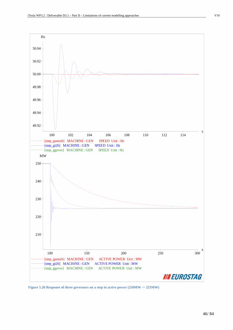
iTesla WP3.2 : Deliverable D3.1 – Part II – Limitations of current modelling approaches V10
46/ 84
100 150 200 250 300
210
220
230
240
250
s
MW
[step_gasturb] MACHINE : GEN ACTIVE POWER Unit : MW[step_gt26] MACHINE : GEN ACTIVE POWER Unit : MW[step_ggover] MACHINE : GEN ACTIVE POWER Unit : MW
100 102 104 106 108 110 112 114
49.92
49.94
49.96
49.98
50.00
50.02
50.04
s
Hz
[step_gasturb] MACHINE : GEN SPEED Unit : Hz[step_gt26] MACHINE : GEN SPEED Unit : Hz[step_ggover] MACHINE : GEN SPEED Unit : Hz
Figure 5.20 Response of three governors on a step in active power (250MW -> 225MW)
iTesla WP3.2 : Deliverable D3.1 – Part II – Limitations of current modelling approaches V10
47/ 84
5.3.6. Gas Turbine Models: Conclusions
A large number of generic gas turbine models are available in the literature. In this document, the GAST, Rowen, WECC, CIGRE and IEEE models are discussed. These generic models are meant to be applicable to a wide range of heavy-duty gas turbines. They can be considered as standard models. Instead of building a dedicated model for each gas turbine in his system, the TSO can select one of the standard models for all the gas turbines and use the appropriate parameters. The choice of the standard model is very important, as can be seen from Table 5.I and Table 5.II: it determines for which studies the model can be used. For instance, using the IEEE model in islanding studies is a sure way of obtaining wrong results, as the acceleration control is not included in the model. A model such as the CIGRE or Rowen model contains all important systems and can be used in a wide variety of power system studies. In a last section, a specific model is discussed. The Alstom GT26 turbine model is taken as example and its results are compared with other turbine models. Turbine models act in different ways and correct estimation of the behaviour of the machine is needed in order to select the correct turbine model. Generic models can offer a solution, in case no specific information is available.
5.4. Conclusions
With the above example of gas turbines, it is demonstrated that care has to be taken when using standard models for various power system components. Although the controls of gas turbines are typically complex, the same conclusions can be extended to other power system components. Standard models are sometimes developed with a certain type or brand in mind. Its behaviour can be labelled as a typical response; however particularities of the model and the accompanied standard parameters must be verified and, if possible, compared to the response of the actual system to be modelled.
6. PHYSICAL VS MATHEMATICAL MODELS Modelling of power system equipment is based on the physical structure and operating principles of the device. For gas turbine for instance, the actual control loops such as acceleration and temperature control are also found in the model. The disadvantage is that some assumptions are inherently made while modelling power system equipment. It is for instance possible that a gas turbine model does not have a representation of temperature control. Hence, using physical models can introduce limitations. The alternative is to use mathematical system identification techniques to obtain a model. No knowledge on the physical structure of the model is then needed. However, enough measurements have to be available and most system identification techniques have some limitations such as difficulty of coping with complex nonlinear hybrid systems.
7. CONCLUSIONS AND RECOMMENDATIONS There are a plethora of potential approximations and assumptions in the power system models that can lead to errors.
iTesla WP3.2 : Deliverable D3.1 – Part II – Limitations of current modelling approaches V10
48/ 84
It is shown that equation-based modelling could be a viable alternative in the future to input-output modelling for power system applications. The simulation results show that very similar results can be obtained in EUROSTAG and MODELICA. Both approaches have their limitations, advantages, and disadvantages. At present, some disadvantages of equation-based modelling remain. A dedicated research effort is needed to overcome the difficulties of equation-based modelling and simulation of power systems. Tasks WP3.3 and WP3.4, which rely heavily on MODELICA, should take into account the knowledge gained on the advantages and disadvantages of equation-based modelling. The aggregation process will normally assume a specific load dispatch between the individual units. This dispatch will change in the real system, causing the aggregation to be less accurate. Moreover, the different voltages at the individual units cannot be taken into account. However, aggregation is a must in current power system analysis. It is therefore recommended to take great care in developing robust aggregated models that can be used in a wide range of operating conditions. This task will be performed in WP3.4. It is demonstrated that care has to be taken when using standard models for various power system components. The results obtained with standard and custom models can be totally different. Particularities of the model and the accompanied standard parameters must be verified and, if possible, compared to the response of the actual system to be modelled. Standard models and parameters should not be used without verification. Using mathematical models instead of physical models could have advantages. However, a considerable research effort is needed to develop methods that can handle nonlinear, hybrid power system equipment models, and to show that the results can be trusted. This topic could be further explored in WP3.3.
8. BIBLIOGRAPHY
[1] Modelica Association, “Modelica® - A Unified Object-Oriented Language for Systems Modeling v3.3,” May 2012. [Online]. Available: https://www.modelica.org/documents/ModelicaSpec33.pdf.
[2] P. Fritzson, Principles of Object-Oriented Modeling and Simulation with Modelica 2.1, Wiley-IEEE Press, 2004.
[3] E. Muljadi, S. Pasupulati, A. Ellis, D. Kosterov y IEEE, «Method of Equivalencing for a Large Wind Power Plant with Multiple Turbine Representation,» de IEEE Power & Energy Society General Meeting, 2008.
[4] J. Brochu, C. Larose and R. Gagnon, “Generic Equivalent Collector System Parameters for Large Wind Power Plants,” IEEE Transactions on Energy Conversion, vol. 26, no. 2, p. 542–549, 2011.
[5] “Load Representation for Dynamic Performance Analysis of Power Systems,” IEEE Transactions on Power Systems, vol. 8, no. 2, p. 472–482, 1993.
[6] «Standard load models for power flow and dynamic performance simulation,» IEEE Transactions on Power Systems, vol. 10, nº 3, p. 1302–1313, 1995.
[7] "Task Force 25 of Advisory Group 02 of Study Committee 39", “Modelling of gas turbines and steam turbines in combined-cycle power plants,” 2003.
[8] S. Yee, J. Milanovic and F. Hughes, “Overview and comparative analysis of gas turbine models for system stability studies,” Power Systems, IEEE Transactions on, vol. 23, no. 1, pp. 108-118, 2008.
iTesla WP3.2 : Deliverable D3.1 – Part II – Limitations of current modelling approaches V10
49/ 84
[9] “PSS/E User Manual”.
[10] W. I. Rowen, «Simplified Mathematical Representations of Heavy-Duty Gas Turbines,» Journal of Engineering for Power, vol. 105, pp. 865-869, 1983.
[11] W. I. Rowen, «Rowen - Simplified Mathematical Representations of Single Shaft Gas Turbines in Mechanical Drive Service,» Turbomachinery International, pp. 26-32, July/August 1992.
[12] L. Pereira, J. Undrill, D. Kosterev, D. Davies and S. Patterson, “A new thermal governor modeling approach in the WECC,” Power Systems, IEEE Transactions on, vol. 18, no. 2, pp. 819-829, may 2003.
[13] “Dynamic models for combined cycle plants in power system studies,” Power Systems, IEEE Transactions on, vol. 9, no. 3, pp. 1698-1708, aug 1994.
[14] P. Pourbeik, «The dependance of gas turbine power output on system frequency and ambient conditions,» CIGRE Session, nº 38-101, p. 5, 2002.
[15] Tase Force 25 of Advisory Group 02 of Study Committee 39, «Modeling of gas turbines and steam turbines in combined--cycle power plants,» 2003.
[16] M. D. Group, «Modelica – A Unified Object-Oriented Language for Physical Systems Modeling, Language Specification,» 1999. [En línea]. Available: http://www.modelica.org/current/modelicaspec12norev.pdf.
[17] “ModelicaML description and documentation,” [Online]. Available: https://www.openmodelica.org/index.php/developer/tools/134.
[18] “Dymola product description,” [Online]. Available: http://www.modelon.com/products/dymola/.
[19] Modelon distribution group, “Electric power Library description,” [Online]. Available: http://www.modelon.com/products/modelica-libraries/electrical-power-library/.
[20] Modelica Association, “Object Stab,” january 2007. [Online]. Available: https://www.modelica.org/libraries/ObjectStab.
[21] Pegase, «D5.2: Proof of concept for an open simulation and model sharing framework validated on a medium size power system,» [En línea]. Available: http://fp7-pegase.eu/var/plain_site/storage/original/application/1dd0b1e7f732968a00b01e8fe59f446a.pdf.
[22] “Dymola export features,” [Online]. Available: http://www.3ds.com/products/catia/portfolio/dymola/dymola-product-line/code-and-model-export/.
[23] D. S. AB, «Dymola - Dynamic Modeling Laboratory – Chapter 6 “Appendix - Installation”».
[24] T. Blochwitz y e. al, «The Functional Mockup Interface for Tool Independent Exchange of Simulation Models,» Dresden, 2011.
[25] “Functional Mockup Interface,” [Online]. Available: https://www.fmi-standard.org/tools.
[26] “FMI Toolbox for Matlab,” [Online]. Available: http://www.modelon.com/products/fmi-toolbox-for-matlab/.
[27] Modelica Design Group, “Modelica and the Modelica Association,” [Online]. Available: https://www.modelica.org/.
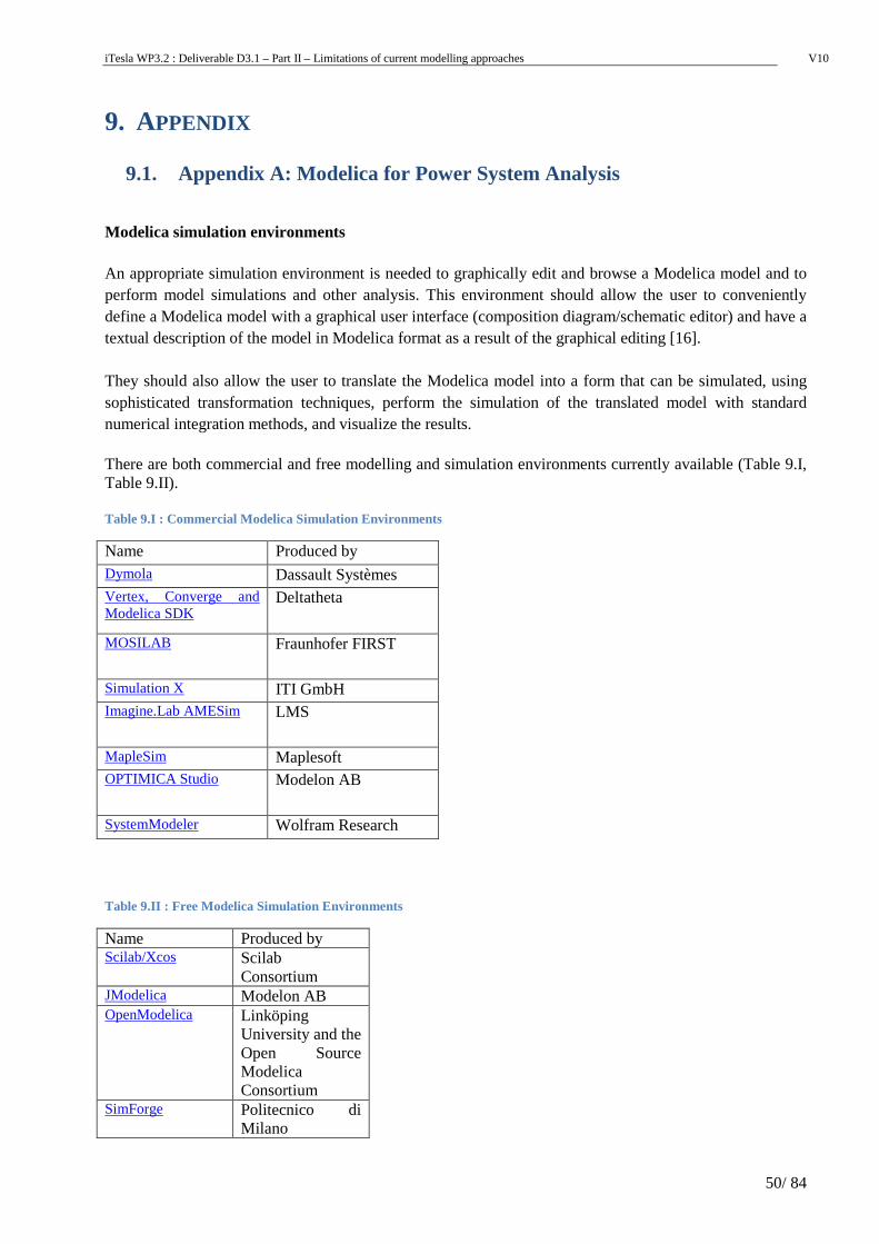
iTesla WP3.2 : Deliverable D3.1 – Part II – Limitations of current modelling approaches V10
50/ 84
9. APPENDIX
9.1. Appendix A: Modelica for Power System Analysis
Modelica simulation environments An appropriate simulation environment is needed to graphically edit and browse a Modelica model and to perform model simulations and other analysis. This environment should allow the user to conveniently define a Modelica model with a graphical user interface (composition diagram/schematic editor) and have a textual description of the model in Modelica format as a result of the graphical editing [16]. They should also allow the user to translate the Modelica model into a form that can be simulated, using sophisticated transformation techniques, perform the simulation of the translated model with standard numerical integration methods, and visualize the results. There are both commercial and free modelling and simulation environments currently available (Table 9.I, Table 9.II). Table 9.I : Commercial Modelica Simulation Environments
Name Produced by Dymola Dassault Systèmes Vertex, Converge and Modelica SDK
Deltatheta
MOSILAB Fraunhofer FIRST
Simulation X ITI GmbH Imagine.Lab AMESim LMS
MapleSim Maplesoft OPTIMICA Studio Modelon AB
SystemModeler Wolfram Research
Table 9.II : Free Modelica Simulation Environments
Name Produced by Scilab/Xcos Scilab
Consortium JModelica Modelon AB OpenModelica Linköping
University and the Open Source Modelica Consortium
SimForge Politecnico di Milano

iTesla WP3.2 : Deliverable D3.1 – Part II – Limitations of current modelling approaches V10
51/ 84
Modelica is a non-proprietary, object-oriented, equation based language to conveniently model complex physical systems. The Modelica Modeling Language (ModelicaML) is a graphical modeling language for the description of time-continuous and time-discrete/event-based system dynamics. ModelicaML is defined as an extended subset of the OMG Unified Modeling Language (UML). This subset enables the generation of executable Modelica code [17]. Dymola is a general-purpose simulation tool based on the Modelica language [1]. Dymola is based on the Modelica open standard. Modelica is an object-oriented, declarative, multi-domain modeling language for component-oriented modeling of complex systems, e.g., systems containing mechanical, electrical, electronic, hydraulic, thermal, control, electric power or process-oriented subcomponents [18] Dymola is a modelling and simulation tool with a Modelica translator able to perform all necessary symbolic transformations for large systems (more than 100000 equations) as well as for real time applications. It includes a graphical editor for model editing and browsing, and a simulation environment. It also provides convenient interfaces to Matlab and the popular block diagram simulator Simulink. For example, a Modelica model can be transformed into a SIMULINK S-function which can be simulated in Simulink as an input/output block. Within Dymola, for power system simulations it is possible to use Electric Power Library (EPL) [19]. EPL provides a framework for efficient modeling, simulation and analysis of electric power systems, including AC three phase systems, AC one phase systems, and DC systems. The models can be used in both steady state and transient mode for simulation and initialization. Some of the main implementations are free/opensource with a community and research groups support (OpenModelica, Scilab/Xcos, etc.), and other are closed commercial products (Dymola). It seems there is a growing interest in the industry in this class of solutions, reflected in the fact that main mathematical tools are incorporating interfaces to deal with it (Mathematica “SystemModeler”, Matlab “FMI Toolbox”, Maple “MapleSim”) and increasing number of research papers in diverse industrial sectors (robotics, car design, etc). There is also a Power System library called ObjectStab for voltage and transient stability analysis and simulation written in Modelica [20], intended for use with the commercial simulation environment, Dymola from Dynasim AB, which is not an open tool. Evaluation of Modelica-based tools for off-line simulation In order to evaluate capabilities of Modelica language and Modelica-based software tools for power system simulation, several tests were carried out (Figure 9.1).
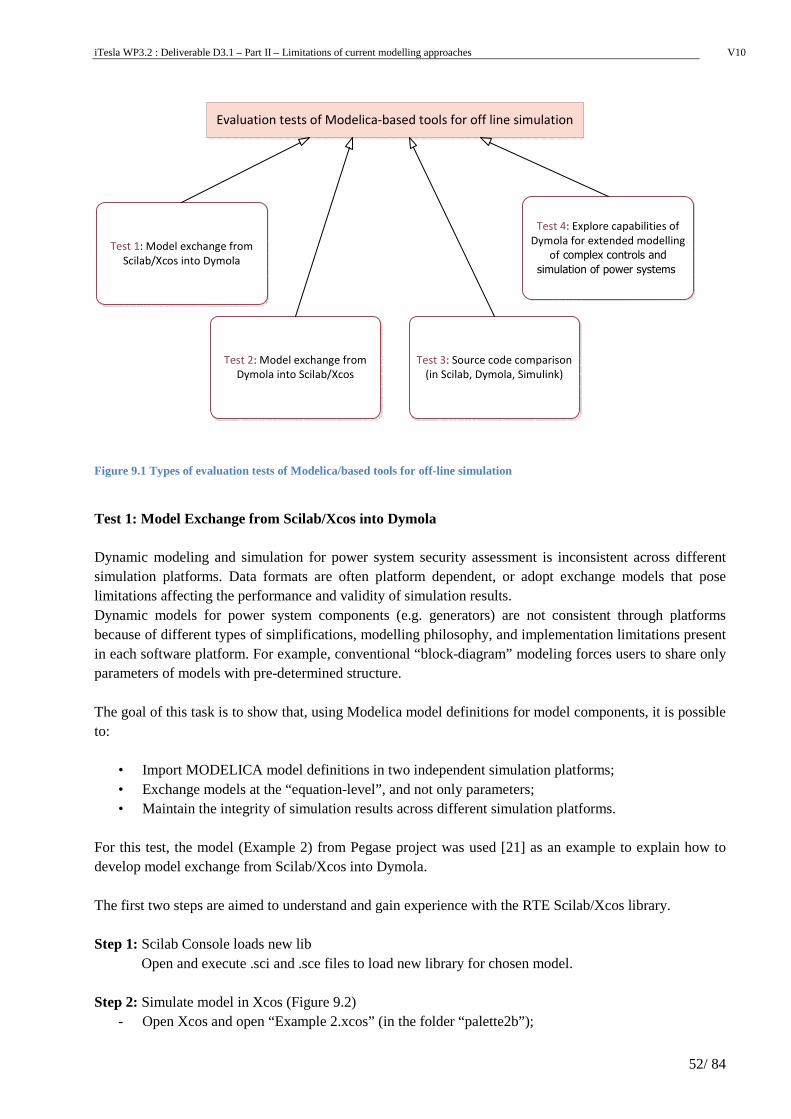
iTesla WP3.2 : Deliverable D3.1 – Part II – Limitations of current modelling approaches V10
52/ 84
Test 2: Model exchange from
Dymola into Scilab/Xcos
Test 1: Model exchange from
Scilab/Xcos into Dymola
Test 3: Source code comparison
(in Scilab, Dymola, Simulink)
Test 4: Explore capabilities of
Dymola for extended modelling
of complex controls and
simulation of power systems
Evaluation tests of Modelica‐based tools for off line simulation
Figure 9.1 Types of evaluation tests of Modelica/based tools for off-line simulation
Test 1: Model Exchange from Scilab/Xcos into Dymola Dynamic modeling and simulation for power system security assessment is inconsistent across different simulation platforms. Data formats are often platform dependent, or adopt exchange models that pose limitations affecting the performance and validity of simulation results. Dynamic models for power system components (e.g. generators) are not consistent through platforms because of different types of simplifications, modelling philosophy, and implementation limitations present in each software platform. For example, conventional “block-diagram” modeling forces users to share only parameters of models with pre-determined structure. The goal of this task is to show that, using Modelica model definitions for model components, it is possible to:
• Import MODELICA model definitions in two independent simulation platforms; • Exchange models at the “equation-level”, and not only parameters; • Maintain the integrity of simulation results across different simulation platforms.
For this test, the model (Example 2) from Pegase project was used [21] as an example to explain how to develop model exchange from Scilab/Xcos into Dymola. The first two steps are aimed to understand and gain experience with the RTE Scilab/Xcos library. Step 1: Scilab Console loads new lib
Open and execute .sci and .sce files to load new library for chosen model. Step 2: Simulate model in Xcos (Figure 9.2)
- Open Xcos and open “Example 2.xcos” (in the folder “palette2b”);
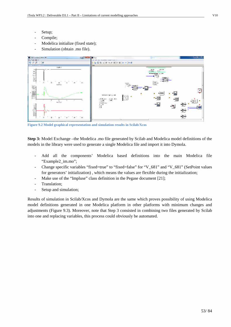
iTesla WP3.2 : Deliverable D3.1 – Part II – Limitations of current modelling approaches V10
53/ 84
- Setup; - Compile; - Modelica initialize (fixed state); - Simulation (obtain .mo file).
Figure 9.2 Model graphical representation and simulation results in Scilab/Xcos
Step 3: Model Exchange –the Modelica .mo file generated by Scilab and Modelica model definitions of the models in the library were used to generate a single Modelica file and import it into Dymola.
- Add all the components’ Modelica based definitions into the main Modelica file “Example2_im.mo”;
- Change specific variables “fixed=true” to “fixed=false” for “V_681” and “V_681” (SetPoint values for generators’ initialization) , which means the values are flexible during the initialization;
- Make use of the “Impluse” class definition in the Pegase document [21]; - Translation; - Setup and simulation;
Results of simulation in Scilab/Xcos and Dymola are the same which proves possibility of using Modelica model definitions generated in one Modelica platform in other platforms with minimum changes and adjustments (Figure 9.3). Moreover, note that Step 3 consisted in combining two files generated by Scilab into one and replacing variables, this process could obviously be automated.
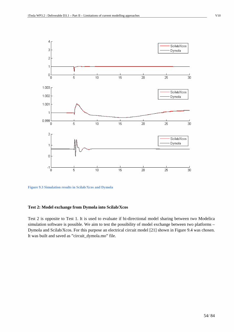
iTesla WP3.2 : Deliverable D3.1 – Part II – Limitations of current modelling approaches V10
54/ 84
Figure 9.3 Simulation results in Scilab/Xcos and Dymola
Test 2: Model exchange from Dymola into Scilab/Xcos Test 2 is opposite to Test 1. It is used to evaluate if bi-directional model sharing between two Modelica simulation software is possible. We aim to test the possibility of model exchange between two platforms – Dymola and Scilab/Xcos. For this purpose an electrical circuit model [21] shown in Figure 9.4 was chosen. It was built and saved as ”circuit_dymola.mo” file.
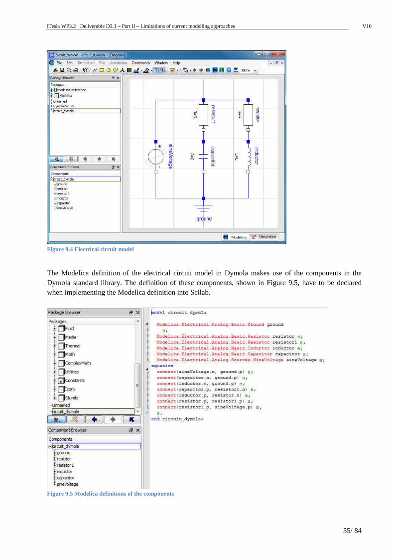
iTesla WP3.2 : Deliverable D3.1 – Part II – Limitations of current modelling approaches V10
55/ 84
Figure 9.4 Electrical circuit model
The Modelica definition of the electrical circuit model in Dymola makes use of the components in the Dymola standard library. The definition of these components, shown in Figure 9.5, have to be declared when implementing the Modelica definition into Scilab.
Figure 9.5 Modelica definitions of the components
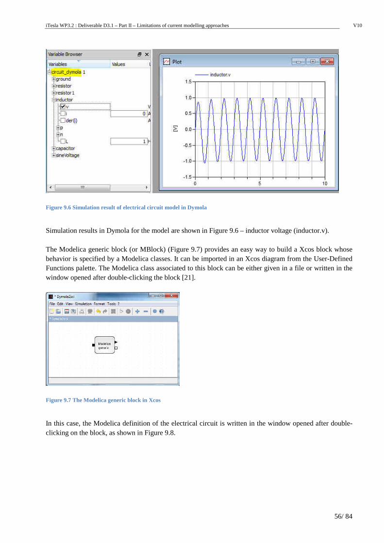
iTesla WP3.2 : Deliverable D3.1 – Part II – Limitations of current modelling approaches V10
56/ 84
Figure 9.6 Simulation result of electrical circuit model in Dymola
Simulation results in Dymola for the model are shown in Figure 9.6 – inductor voltage (inductor.v). The Modelica generic block (or MBlock) (Figure 9.7) provides an easy way to build a Xcos block whose behavior is specified by a Modelica classes. It can be imported in an Xcos diagram from the User-Defined Functions palette. The Modelica class associated to this block can be either given in a file or written in the window opened after double-clicking the block [21].
Figure 9.7 The Modelica generic block in Xcos
In this case, the Modelica definition of the electrical circuit is written in the window opened after double-clicking on the block, as shown in Figure 9.8.
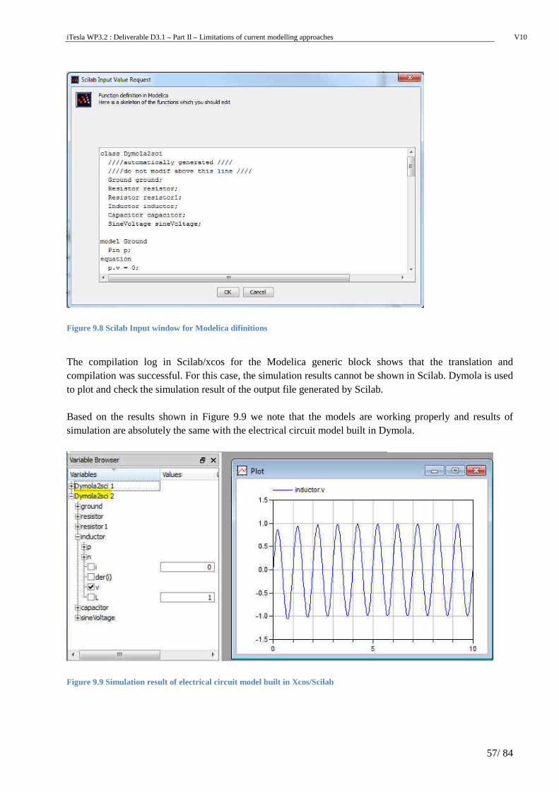
iTesla WP3.2 : Deliverable D3.1 – Part II – Limitations of current modelling approaches V10
57/ 84
Figure 9.8 Scilab Input window for Modelica difinitions
The compilation log in Scilab/xcos for the Modelica generic block shows that the translation and compilation was successful. For this case, the simulation results cannot be shown in Scilab. Dymola is used to plot and check the simulation result of the output file generated by Scilab. Based on the results shown in Figure 9.9 we note that the models are working properly and results of simulation are absolutely the same with the electrical circuit model built in Dymola.
Figure 9.9 Simulation result of electrical circuit model built in Xcos/Scilab
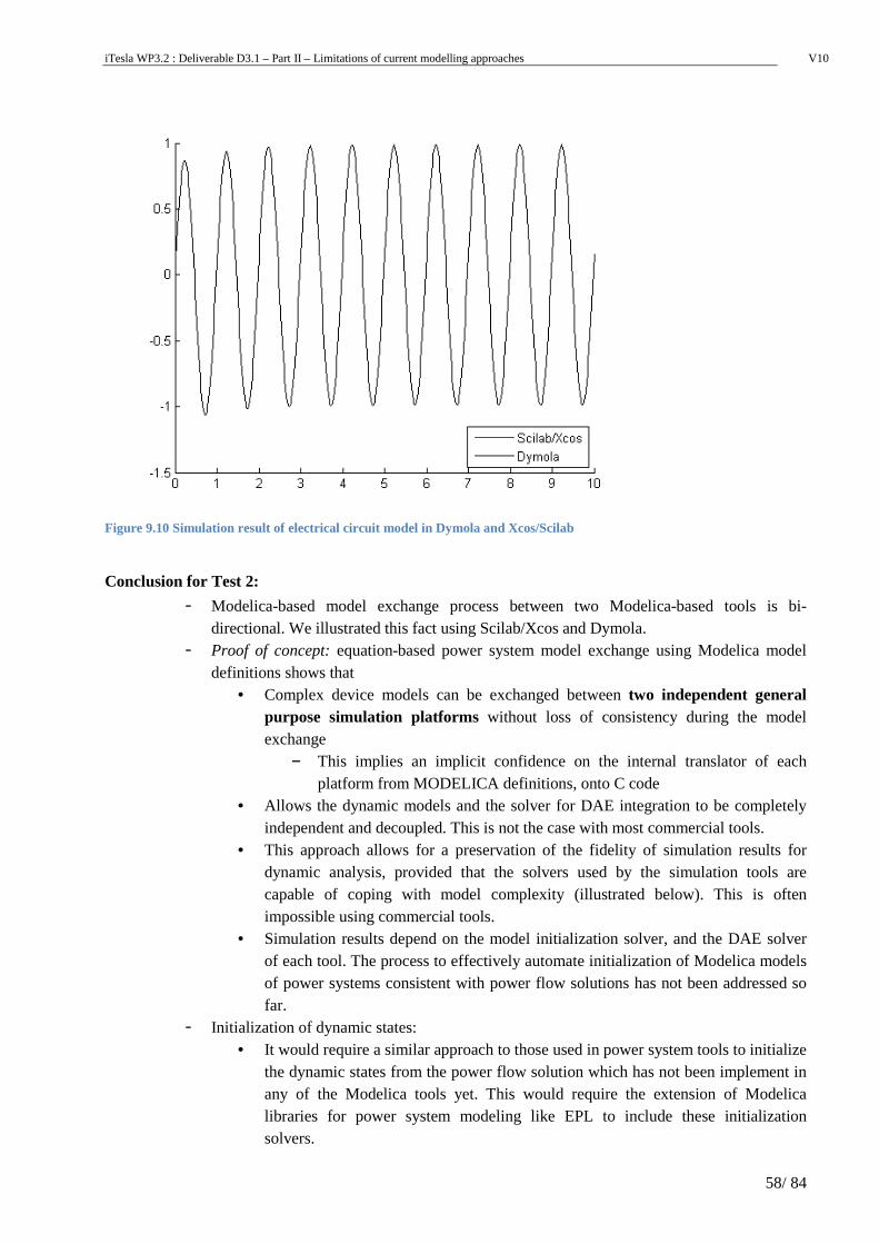
iTesla WP3.2 : Deliverable D3.1 – Part II – Limitations of current modelling approaches V10
58/ 84
Figure 9.10 Simulation result of electrical circuit model in Dymola and Xcos/Scilab
Conclusion for Test 2:
- Modelica-based model exchange process between two Modelica-based tools is bi-directional. We illustrated this fact using Scilab/Xcos and Dymola.
- Proof of concept: equation-based power system model exchange using Modelica model definitions shows that
• Complex device models can be exchanged between two independent general purpose simulation platforms without loss of consistency during the model exchange – This implies an implicit confidence on the internal translator of each
platform from MODELICA definitions, onto C code • Allows the dynamic models and the solver for DAE integration to be completely
independent and decoupled. This is not the case with most commercial tools. • This approach allows for a preservation of the fidelity of simulation results for
dynamic analysis, provided that the solvers used by the simulation tools are capable of coping with model complexity (illustrated below). This is often impossible using commercial tools.
• Simulation results depend on the model initialization solver, and the DAE solver of each tool. The process to effectively automate initialization of Modelica models of power systems consistent with power flow solutions has not been addressed so far.
- Initialization of dynamic states: • It would require a similar approach to those used in power system tools to initialize
the dynamic states from the power flow solution which has not been implement in any of the Modelica tools yet. This would require the extension of Modelica libraries for power system modeling like EPL to include these initialization solvers.
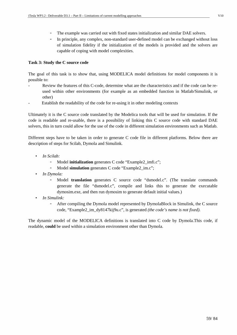
iTesla WP3.2 : Deliverable D3.1 – Part II – Limitations of current modelling approaches V10
59/ 84
- The example was carried out with fixed states initialization and similar DAE solvers. - In principle, any complex, non-standard user-defined model can be exchanged without loss
of simulation fidelity if the initialization of the models is provided and the solvers are capable of coping with model complexities.
Task 3: Study the C source code The goal of this task is to show that, using MODELICA model definitions for model components it is possible to: - Review the features of this C-code, determine what are the characteristics and if the code can be re-
used within other environments (for example as an embedded function in Matlab/Simulink, or other)
- Establish the readability of the code for re-using it in other modeling contexts Ultimately it is the C source code translated by the Modelica tools that will be used for simulation. If the code is readable and re-usable, there is a possibility of linking this C source code with standard DAE solvers, this in turn could allow for the use of the code in different simulation environments such as Matlab. Different steps have to be taken in order to generate C code file in different platforms. Below there are description of steps for Scilab, Dymola and Simulink.
• In Scilab: - Model initialization generates C code “Example2_imfi.c”; - Model simulation generates C code “Example2_im.c”;
• In Dymola: - Model translation generates C source code “dsmodel.c”. (The translate commands
generate the file “dsmodel.c”, compile and links this to generate the executable dymosim.exe, and then run dymosim to generate default initial values.)
• In Simulink: - After compiling the Dymola model represented by DymolaBlock in Simulink, the C source
code, “Example2_im_dy8147kij9u.c”, is generated (the code’s name is not fixed). The dynamic model of the MODELICA definitions is translated into C code by Dymola.This code, if readable, could be used within a simulation environment other than Dymola.
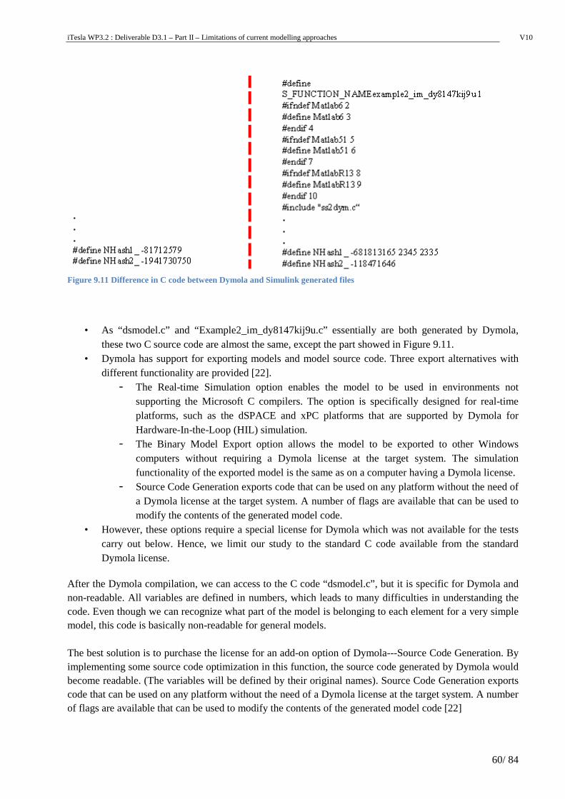
iTesla WP3.2 : Deliverable D3.1 – Part II – Limitations of current modelling approaches V10
60/ 84
Figure 9.11 Difference in C code between Dymola and Simulink generated files
• As “dsmodel.c” and “Example2_im_dy8147kij9u.c” essentially are both generated by Dymola, these two C source code are almost the same, except the part showed in Figure 9.11.
• Dymola has support for exporting models and model source code. Three export alternatives with different functionality are provided [22]. - The Real-time Simulation option enables the model to be used in environments not
supporting the Microsoft C compilers. The option is specifically designed for real-time platforms, such as the dSPACE and xPC platforms that are supported by Dymola for Hardware-In-the-Loop (HIL) simulation.
- The Binary Model Export option allows the model to be exported to other Windows computers without requiring a Dymola license at the target system. The simulation functionality of the exported model is the same as on a computer having a Dymola license.
- Source Code Generation exports code that can be used on any platform without the need of a Dymola license at the target system. A number of flags are available that can be used to modify the contents of the generated model code.
• However, these options require a special license for Dymola which was not available for the tests carry out below. Hence, we limit our study to the standard C code available from the standard Dymola license.
After the Dymola compilation, we can access to the C code “dsmodel.c”, but it is specific for Dymola and non-readable. All variables are defined in numbers, which leads to many difficulties in understanding the code. Even though we can recognize what part of the model is belonging to each element for a very simple model, this code is basically non-readable for general models. The best solution is to purchase the license for an add-on option of Dymola---Source Code Generation. By implementing some source code optimization in this function, the source code generated by Dymola would become readable. (The variables will be defined by their original names). Source Code Generation exports code that can be used on any platform without the need of a Dymola license at the target system. A number of flags are available that can be used to modify the contents of the generated model code [22]
iTesla WP3.2 : Deliverable D3.1 – Part II – Limitations of current modelling approaches V10
61/ 84
• Source Code Generation allows export of readable and well-documented code facilitating inspection, debugging, profiling, etc. This makes this export option suitable for advanced model-based applications, such as rapid prototyping.
• The Source Code Generation option includes the functionality provided by Real-time Simulation (without the inline integration restriction) and Binary Model Export when models are translated in Dymola or Simulink.
• The Binary Model Export and Source Code Generation options both allow export of symbol table information, e.g., model structure, variable names, types, and units as an XML file.
To execute or run a file from MS-DOS you must run an executable file, which are .exe, .bat, or .com files [19]. So that it is possible to start Dymola by using the Windows command prompt and enter the directory of the executable file, for instance, “C:\Program Files (x86)\Dymola 2012\bin\Dymola.exe”. Another case is when you want a more detailed description for a license server error, you can access FLEXnet Publisher error codes by enter “C:\Program Files (x86)\Dymola 2012\bin\Dymola.exe/FLEXlmDiag” .
• However, in the Windows command prompt no commands could be used to realize translating and doing simulation for a model file. While simulation from the command line is available in Linux operation system [23].
• There is a command line in Dymola where the user could translate models and do simulation by typing command, as marked in Figure 9.12. But it seems not quite meaningful as all the operation could be done by GUI.
Figure 9.12 Dymola command line
Test 4: Explore the capabilities of Dymola for extended modeling of complex controls and simulation of power systems
The goal of this test is to investigate limitations of using Modelica-based tools for power system simulation. The next steps should be done to achive the goal:
- Eliminate filters between pulse blocks in the Scilab/Xcos and evaluate if this can be modeled in a different fashion within Dymola using discrete blocks. (Implementation of two sequential discrete events is not possible in Scilab/Xcos, and is required for special models used by RTE)
- Create a large-scale power system network similar to the “string network” used in the PEGASE project. Establish what the system size limits for simulation using Dymola are.
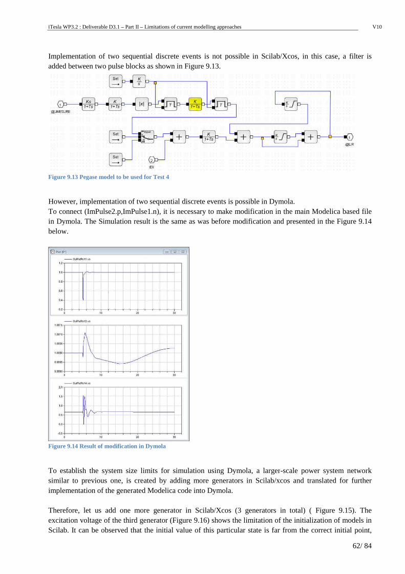
iTesla WP3.2 : Deliverable D3.1 – Part II – Limitations of current modelling approaches
Implementation of two sequential discrete events is not possible in Scilab/Xcos, in this case, a filter is added between two pulse blocks as shown in
Figure 9.13 Pegase model to be used for Test 4
However, implementation of two sequential discrete events is possible in Dymola. To connect (ImPulse2.p,ImPulse1.n), in Dymola. The Simulation result is the same as was before modification and presented in the below.
Figure 9.14 Result of modification in Dymola
To establish the system size limits for simulation using Dymola, a largersimilar to previous one, is created by adding more generators in Scilab/xcos and translated for further implementation of the generated Modelica code into Dymola. Therefore, let us add one more generator in Scilab/Xcos (3 generators in total) (excitation voltage of the third generator (Scilab. It can be observed that the initial value of this particular state is far from the correct initial point,
Limitations of current modelling approaches
Implementation of two sequential discrete events is not possible in Scilab/Xcos, in this case, a filter is added between two pulse blocks as shown in Figure 9.13.
Pegase model to be used for Test 4
However, implementation of two sequential discrete events is possible in Dymola. To connect (ImPulse2.p,ImPulse1.n), it is necessary to make modification in the main Modelica based file in Dymola. The Simulation result is the same as was before modification and presented in the
Result of modification in Dymola
To establish the system size limits for simulation using Dymola, a larger-scale power system network created by adding more generators in Scilab/xcos and translated for further
implementation of the generated Modelica code into Dymola.
Therefore, let us add one more generator in Scilab/Xcos (3 generators in total) (excitation voltage of the third generator (Figure 9.16) shows the limitation of the initialization of models in Scilab. It can be observed that the initial value of this particular state is far from the correct initial point,
V10
62/ 84
Implementation of two sequential discrete events is not possible in Scilab/Xcos, in this case, a filter is
However, implementation of two sequential discrete events is possible in Dymola. it is necessary to make modification in the main Modelica based file
in Dymola. The Simulation result is the same as was before modification and presented in the Figure 9.14
scale power system network created by adding more generators in Scilab/xcos and translated for further
Therefore, let us add one more generator in Scilab/Xcos (3 generators in total) ( Figure 9.15). The limitation of the initialization of models in
Scilab. It can be observed that the initial value of this particular state is far from the correct initial point,
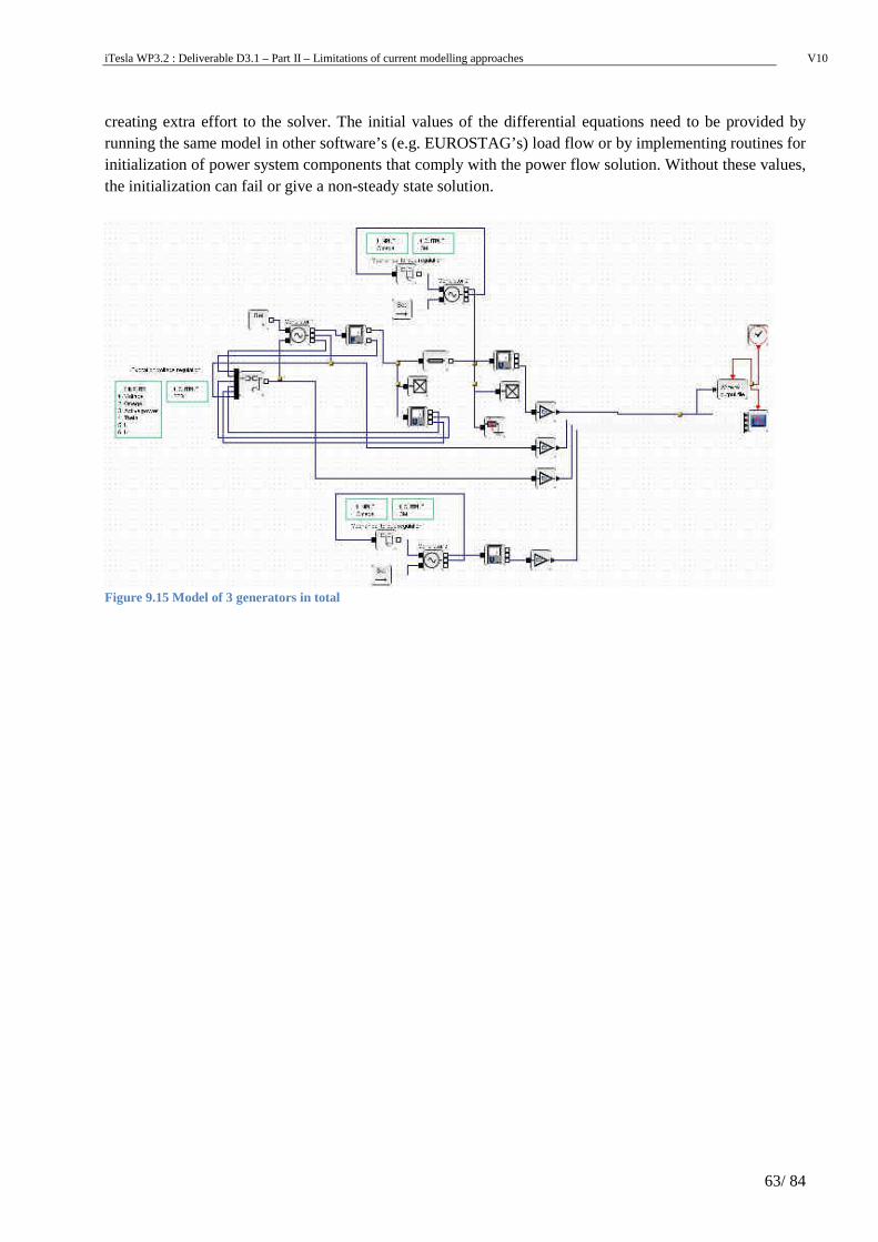
iTesla WP3.2 : Deliverable D3.1 – Part II – Limitations of current modelling approaches V10
63/ 84
creating extra effort to the solver. The initial values of the differential equations need to be provided by running the same model in other software’s (e.g. EUROSTAG’s) load flow or by implementing routines for initialization of power system components that comply with the power flow solution. Without these values, the initialization can fail or give a non-steady state solution.
Figure 9.15 Model of 3 generators in total
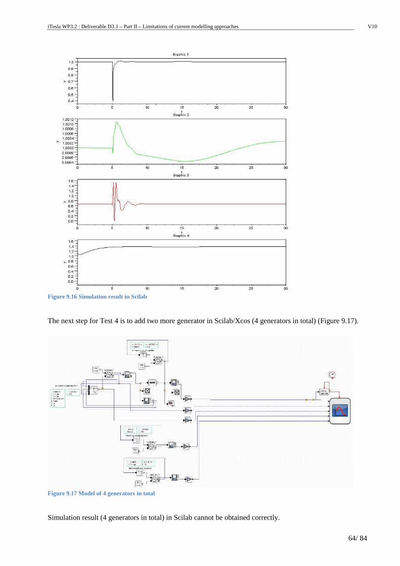
iTesla WP3.2 : Deliverable D3.1 – Part II – Limitations of current modelling approaches V10
64/ 84
Figure 9.16 Simulation result in Scilab
The next step for Test 4 is to add two more generator in Scilab/Xcos (4 generators in total) (Figure 9.17).
Figure 9.17 Model of 4 generators in total
Simulation result (4 generators in total) in Scilab cannot be obtained correctly.
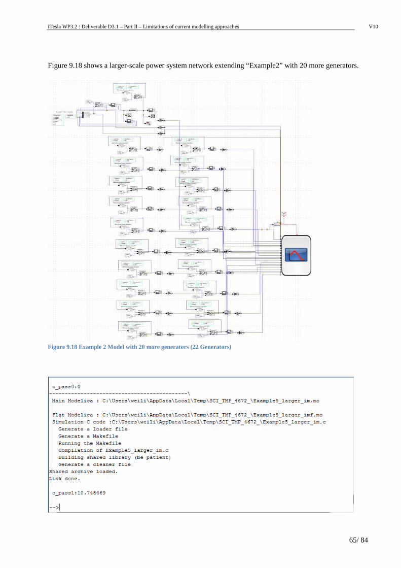
iTesla WP3.2 : Deliverable D3.1 – Part II – Limitations of current modelling approaches V10
65/ 84
Figure 9.18 shows a larger-scale power system network extending “Example2” with 20 more generators.
Figure 9.18 Example 2 Model with 20 more generators (22 Generators)
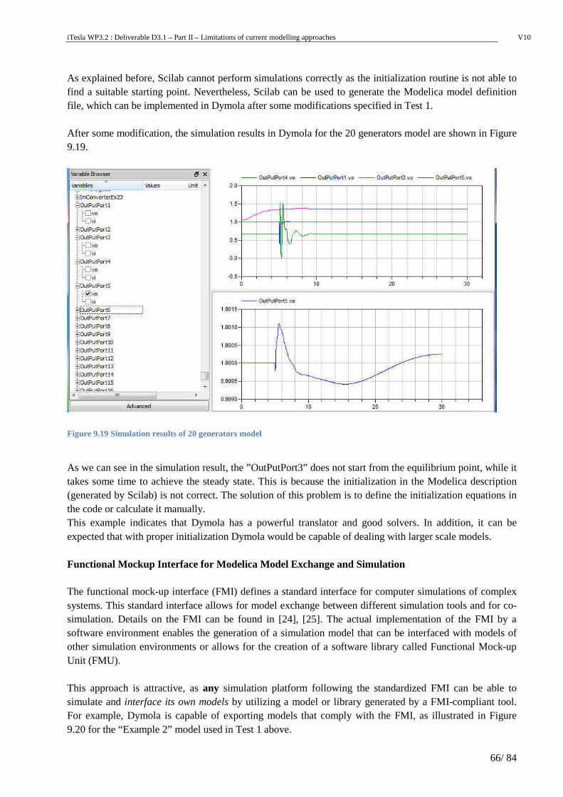
iTesla WP3.2 : Deliverable D3.1 – Part II – Limitations of current modelling approaches V10
66/ 84
As explained before, Scilab cannot perform simulations correctly as the initialization routine is not able to find a suitable starting point. Nevertheless, Scilab can be used to generate the Modelica model definition file, which can be implemented in Dymola after some modifications specified in Test 1. After some modification, the simulation results in Dymola for the 20 generators model are shown in Figure 9.19.
Figure 9.19 Simulation results of 20 generators model
As we can see in the simulation result, the ”OutPutPort3” does not start from the equilibrium point, while it takes some time to achieve the steady state. This is because the initialization in the Modelica description (generated by Scilab) is not correct. The solution of this problem is to define the initialization equations in the code or calculate it manually. This example indicates that Dymola has a powerful translator and good solvers. In addition, it can be expected that with proper initialization Dymola would be capable of dealing with larger scale models. Functional Mockup Interface for Modelica Model Exchange and Simulation The functional mock-up interface (FMI) defines a standard interface for computer simulations of complex systems. This standard interface allows for model exchange between different simulation tools and for co-simulation. Details on the FMI can be found in [24], [25]. The actual implementation of the FMI by a software environment enables the generation of a simulation model that can be interfaced with models of other simulation environments or allows for the creation of a software library called Functional Mock-up Unit (FMU). This approach is attractive, as any simulation platform following the standardized FMI can be able to simulate and interface its own models by utilizing a model or library generated by a FMI-compliant tool. For example, Dymola is capable of exporting models that comply with the FMI, as illustrated in Figure 9.20 for the “Example 2” model used in Test 1 above.
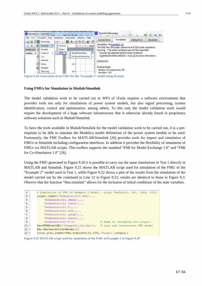
iTesla WP3.2 : Deliverable D3.1 – Part II – Limitations of current modelling approaches V10
67/ 84
Figure 9.20 Generation of an FMU for the “Example 2” model using Dymola
Using FMUs for Simulation in Matlab/Simulink The model validation work to be carried out in WP3 of iTesla requires a software environment that provides tools not only for simulations of power system models, but also signal processing, system identification, control and optimization, among others. To this end, the model validation work would require the development of a huge software infrastructure that is otherwise already found in proprietary software solutions such as Matlab/Simulink. To have the tools available in Matlab/Simulink for the model validation work to be carried out, it is a pre-requisite to be able to simulate the Modelica model definitions of the power system models to be used. Fortunately, the FMI Toolbox for MATLAB/Simulink [26] provides tools for import and simulation of FMUs in Simulink including configuration interfaces. In addition it provides the flexibility of simulation of FMUs via MATLAB scripts. This toolbox supports the standard “FMI for Model Exchange 1.0” and “FMI for Co-Simulation 1.0” [26]. Using the FMU generated in Figure 9.20 it is possible to carry out the same simulations in Test 1 directly in MATLAB and Simulink. Figure 9.21 shows the MATLAB script used for simulation of the FMU of the “Example 2” model used in Test 1, while Figure 9.22 shows a plot of the results from the simulation of the model carried out by the command in Line 12 in Figure 9.21; results are identical to those in Figure 9.3. Observe that the function “fmu.simulate” allows for the inclusion of initial conditions of the state variables.
Figure 9.21 MATLAB script used for simulation of the FMU of Example 2 in Figure 9.20
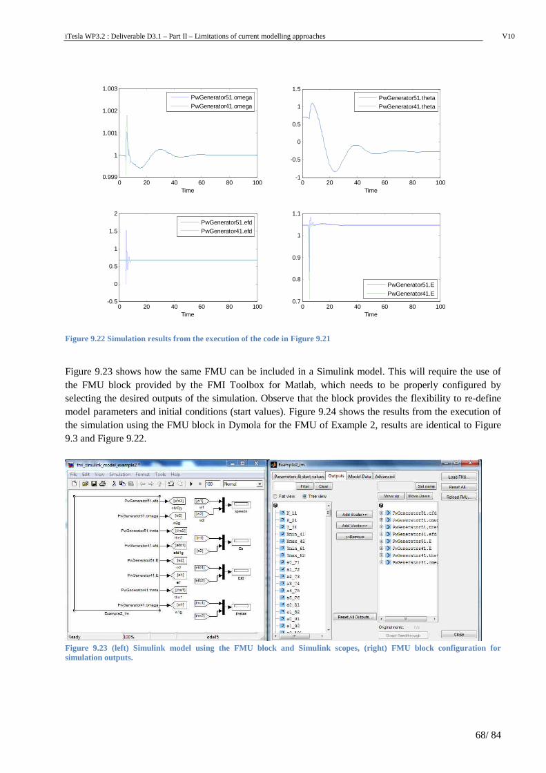
iTesla WP3.2 : Deliverable D3.1 – Part II – Limitations of current modelling approaches V10
68/ 84
Figure 9.22 Simulation results from the execution of the code in Figure 9.21
Figure 9.23 shows how the same FMU can be included in a Simulink model. This will require the use of the FMU block provided by the FMI Toolbox for Matlab, which needs to be properly configured by selecting the desired outputs of the simulation. Observe that the block provides the flexibility to re-define model parameters and initial conditions (start values). Figure 9.24 shows the results from the execution of the simulation using the FMU block in Dymola for the FMU of Example 2, results are identical to Figure 9.3 and Figure 9.22.
Figure 9.23 (left) Simulink model using the FMU block and Simulink scopes, (right) FMU block configuration for simulation outputs.
0 20 40 60 80 1000.999
1
1.001
1.002
1.003
Time
PwGenerator51.omega
PwGenerator41.omega
0 20 40 60 80 100-1
-0.5
0
0.5
1
1.5
Time
PwGenerator51.theta
PwGenerator41.theta
0 20 40 60 80 100-0.5
0
0.5
1
1.5
2
Time
PwGenerator51.efd
PwGenerator41.efd
0 20 40 60 80 1000.7
0.8
0.9
1
1.1
Time
PwGenerator51.E
PwGenerator41.E
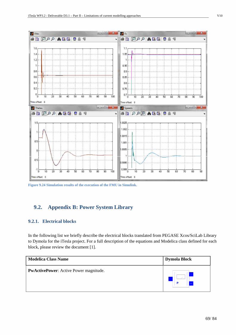
iTesla WP3.2 : Deliverable D3.1 – Part II – Limitations of current modelling approaches V10
69/ 84
Figure 9.24 Simulation results of the execution of the FMU in Simulink.
9.2. Appendix B: Power System Library
9.2.1. Electrical blocks
In the following list we briefly describe the electrical blocks translated from PEGASE Xcos/SciLab Library to Dymola for the iTesla project. For a full description of the equations and Modelica class defined for each block, please review the document [1].
Modelica Class Name Dymola Block
PwActivePower: Active Power magnitude.
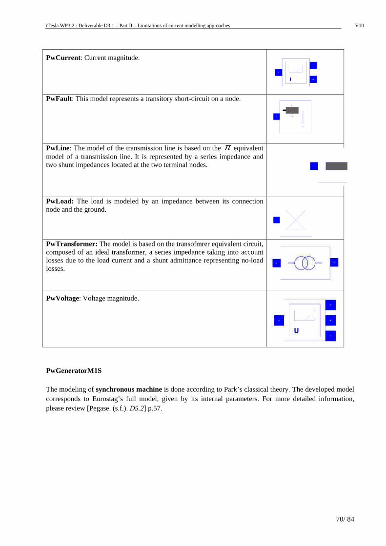
iTesla WP3.2 : Deliverable D3.1 – Part II – Limitations of current modelling approaches V10
70/ 84
PwCurrent : Current magnitude.
PwFault: This model represents a transitory short-circuit on a node.
PwLine: The model of the transmission line is based on the π equivalent model of a transmission line. It is represented by a series impedance and two shunt impedances located at the two terminal nodes.
PwLoad: The load is modeled by an impedance between its connection node and the ground.
PwTransformer: The model is based on the transofmrer equivalent circuit, composed of an ideal transformer, a series impedance taking into account losses due to the load current and a shunt admittance representing no-load losses.
PwVoltage: Voltage magnitude.
PwGeneratorM1S The modeling of synchronous machine is done according to Park’s classical theory. The developed model corresponds to Eurostag’s full model, given by its internal parameters. For more detailed information, please review [Pegase. (s.f.). D5.2] p.57.
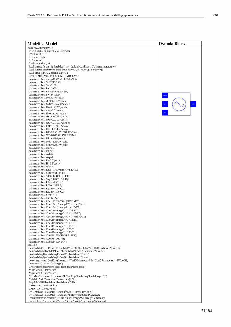
iTesla WP3.2 : Deliverable D3.1 – Part II – Limitations of current modelling approaches V10
71/ 84
Modelica Model Dymola Block class PwGeneratorM1S PwPin sortie(vr(start=1), vi(start=0)); ImPin eefd; ImPin oomega; ImPin ccm; Real cm, efd, ur, ui; Real lambdaf(start=0), lambdad(start=0), lambdaad(start=0), lambdaaq(start=0); Real lambdaq1(start=0), lambdaq2(start=0), id(start=0), iq(start=0); Real theta(start=0), omega(start=0); Real E, Mds, Mqs, Md, Mq, Mi, LMD, LMQ; parameter Real omega0=2*3.14159265*50; parameter Real SNREF=100; parameter Real SN=1150; parameter Real PN=1000; parameter Real yscale=SNREF/SN; parameter Real SNtfo=1300; parameter Real r=0.004*yscale; parameter Real rf=0.00113*yscale; parameter Real Mdv=0.74590*yscale; parameter Real lD=0.12825*yscale; parameter Real mrc=0.0*yscale; parameter Real lf=0.24253*yscale; parameter Real rD=0.01723*yscale; parameter Real rQ1=0.0193*yscale; parameter Real rQ2=0.03923*yscale; parameter Real lQ1=0.08921*yscale; parameter Real lQ2=1.78484*yscale; parameter Real RT=0.000185*SNREF/SNtfo; parameter Real XT=0.00769*SNREF/SNtfo; parameter Real lld=0.219*yscale; parameter Real Md0=2.351*yscale; parameter Real Mq0=2.351*yscale; parameter Real md=0.1; parameter Real mq=0.1; parameter Real snd=6; parameter Real snq=6; parameter Real D=0.0/yscale; parameter Real H=6.3/yscale; parameter Real rtfo=1; parameter Real DET=lf*lD+mrc*lf+mrc*lD; parameter Real Mdif=Md0-Mq0; parameter Real Sdet=lf/DET+lD/DET; parameter Real Slq=1.0/lQ1+1.0/lQ2; parameter Real Lddet=lD/DET; parameter Real Lfdet=lf/DET; parameter Real Lq1inv=1.0/lQ1; parameter Real Lq2inv=1.0/lQ2; parameter Real Sr=r+RT; parameter Real Sx=lld+XT; parameter Real Coef11=rtfo*omega0*rf/Mdv; parameter Real Coef12=rf*omega0*(lD+mrc)/DET; parameter Real Coef13=rf*omega0*mrc/DET; parameter Real Coef14=omega0*rf*lD/DET; parameter Real Coef21=omega0*rD*mrc/DET; parameter Real Coef22=omega0*rD*(lf+mrc)/DET; parameter Real Coef23=omega0*rD*lf/DET; parameter Real Coef31=omega0*rQ1/lQ1; parameter Real Coef32=omega0*rQ1/lQ1; parameter Real Coef41=omega0*rQ2/lQ2; parameter Real Coef42=omega0*rQ2/lQ2; parameter Real Coef51=PN/(SNREF*2*H); parameter Real Coef52=D/(2*H); parameter Real Coef53=1.0/(2*H); equation der(lambdaf)=-efd*Coef11-lambdaf*Coef12+lambdad*Coef13+lambdaad*Coef14; der(lambdad)=lambdaf*Coef21-lambdad*Coef22+lambdaad*Coef23; der(lambdaq1)=-lambdaq1*Coef31+lambdaaq*Coef32; der(lambdaq2)=-lambdaq2*Coef41+lambdaaq*Coef42; der(omega)=cm*Coef51+(1-omega)*Coef52+lambdaad*iq*Coef53-lambdaaq*id*Coef53; der(theta)=(omega-1)*omega0; E=sqrt(lambdaad*lambdaad+lambdaaq*lambdaaq); Mds=Md0/(1+md*E^snd); Mqs=Mq0/(1+mq*E^snq); Mi=Mds*lambdaad*lambdaad/(E*E)+Mqs*lambdaaq*lambdaaq/(E*E); Md=Mi+Mdif*lambdaaq*lambdaaq/(E*E); Mq=Mi-Mdif*lambdaad*lambdaad/(E*E); LMD=1.0/(1.0/Md+Sdet); LMQ=1.0/(1.0/Mq+Slq); 0=-lambdaad+LMD*(id+lambdaf*Lddet+lambdad*Lfdet); 0=-lambdaaq+LMQ*(iq+lambdaq1*Lq1inv+lambdaq2*Lq2inv); 0=sin(theta)*ur-cos(theta)*ui+id*Sr-iq*omega*Sx-omega*lambdaaq; 0=cos(theta)*ur+sin(theta)*ui+iq*Sr+id*omega*Sx+omega*lambdaad;
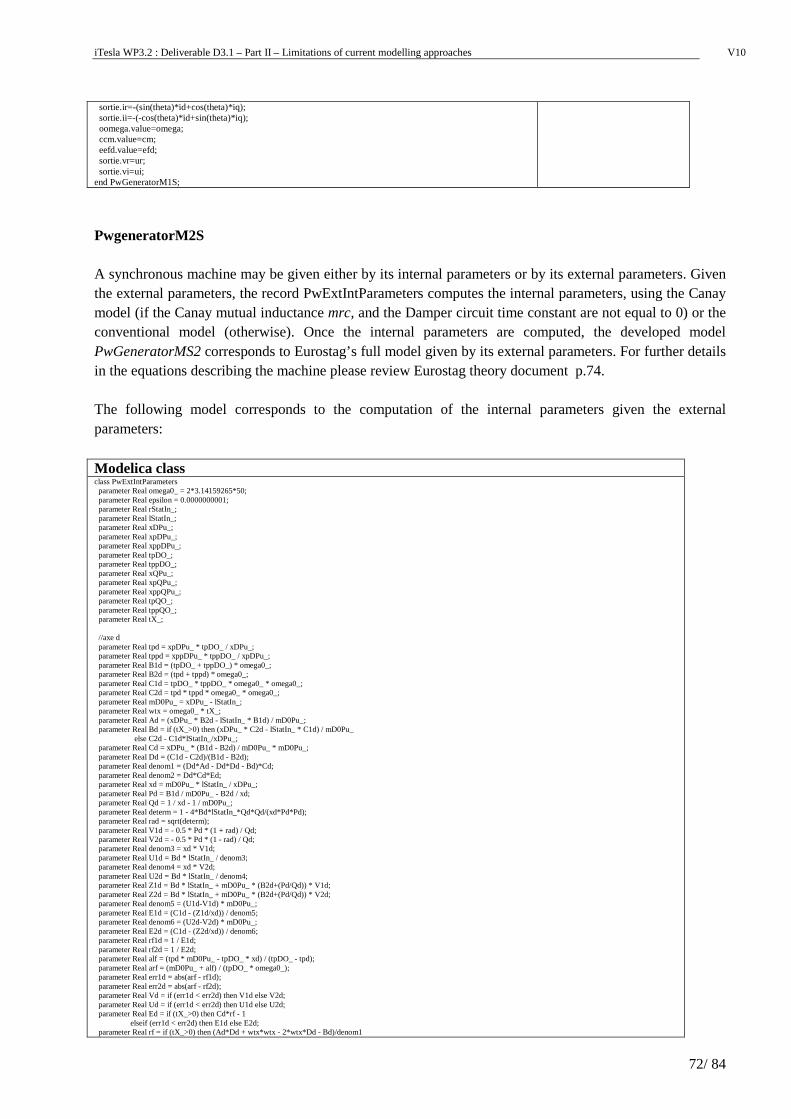
iTesla WP3.2 : Deliverable D3.1 – Part II – Limitations of current modelling approaches V10
72/ 84
sortie.ir=-(sin(theta)*id+cos(theta)*iq); sortie.ii=-(-cos(theta)*id+sin(theta)*iq); oomega.value=omega; ccm.value=cm; eefd.value=efd; sortie.vr=ur; sortie.vi=ui; end PwGeneratorM1S; PwgeneratorM2S A synchronous machine may be given either by its internal parameters or by its external parameters. Given the external parameters, the record PwExtIntParameters computes the internal parameters, using the Canay model (if the Canay mutual inductance mrc, and the Damper circuit time constant are not equal to 0) or the conventional model (otherwise). Once the internal parameters are computed, the developed model PwGeneratorMS2 corresponds to Eurostag’s full model given by its external parameters. For further details in the equations describing the machine please review Eurostag theory document p.74. The following model corresponds to the computation of the internal parameters given the external parameters: Modelica class class PwExtIntParameters parameter Real omega0_ = 2*3.14159265*50; parameter Real epsilon = 0.0000000001; parameter Real rStatIn_; parameter Real lStatIn_; parameter Real xDPu_; parameter Real xpDPu_; parameter Real xppDPu_; parameter Real tpDO_; parameter Real tppDO_; parameter Real xQPu_; parameter Real xpQPu_; parameter Real xppQPu_; parameter Real tpQO_; parameter Real tppQO_; parameter Real tX_; //axe d parameter Real tpd = xpDPu_ * tpDO_ / xDPu_; parameter Real tppd = xppDPu_ * tppDO_ / xpDPu_; parameter Real B1d = (tpDO_ + tppDO_) * omega0_; parameter Real B2d = (tpd + tppd) * omega0_; parameter Real C1d = tpDO_ * tppDO_ * omega0_ * omega0_; parameter Real C2d = tpd * tppd * omega0_ * omega0_; parameter Real mD0Pu_ = xDPu_ - lStatIn_; parameter Real wtx = omega0_ * tX_; parameter Real Ad = (xDPu_ * B2d - lStatIn_ * B1d) / mD0Pu_; parameter Real Bd = if (tX_>0) then (xDPu_ * C2d - lStatIn_ * C1d) / mD0Pu_ else C2d - C1d*lStatIn_/xDPu_; parameter Real Cd = xDPu_ * (B1d - B2d) / mD0Pu_ * mD0Pu_; parameter Real Dd = (C1d - C2d)/(B1d - B2d); parameter Real denom1 = (Dd*Ad - Dd*Dd - Bd)*Cd; parameter Real denom2 = Dd*Cd*Ed; parameter Real xd = mD0Pu_ * lStatIn_ / xDPu_; parameter Real Pd = B1d / mD0Pu_ - B2d / xd; parameter Real Qd = 1 / xd - 1 / mD0Pu_; parameter Real determ = 1 - 4*Bd*lStatIn_*Qd*Qd/(xd*Pd*Pd); parameter Real rad = sqrt(determ); parameter Real V1d = - 0.5 * Pd * (1 + rad) / Qd; parameter Real V2d = - 0.5 * Pd * (1 - rad) / Qd; parameter Real denom3 = xd * V1d; parameter Real U1d = Bd * lStatIn_ / denom3; parameter Real denom4 = xd * V2d; parameter Real U2d = Bd * lStatIn_ / denom4; parameter Real Z1d = Bd * lStatIn_ + mD0Pu_ * (B2d+(Pd/Qd)) * V1d; parameter Real Z2d = Bd * lStatIn_ + mD0Pu_ * (B2d+(Pd/Qd)) * V2d; parameter Real denom5 = (U1d-V1d) * mD0Pu_; parameter Real E1d = (C1d - (Z1d/xd)) / denom5; parameter Real denom6 = (U2d-V2d) * mD0Pu_; parameter Real E2d = (C1d - (Z2d/xd)) / denom6; parameter Real rf1d = 1 / E1d; parameter Real rf2d = 1 / E2d; parameter Real alf = (tpd * mD0Pu_ - tpDO_ * xd) / (tpDO_ - tpd); parameter Real arf = (mD0Pu_ + alf) / (tpDO_ * omega0_); parameter Real err1d = abs(arf - rf1d); parameter Real err2d = abs(arf - rf2d); parameter Real Vd = if (err1d < err2d) then V1d else V2d; parameter Real Ud = if (err1d < err2d) then U1d else U2d; parameter Real Ed = if (tX_>0) then Cd*rf - 1 elseif (err1d < err2d) then E1d else E2d; parameter Real rf = if (tX_>0) then (Ad*Dd + wtx*wtx - 2*wtx*Dd - Bd)/denom1
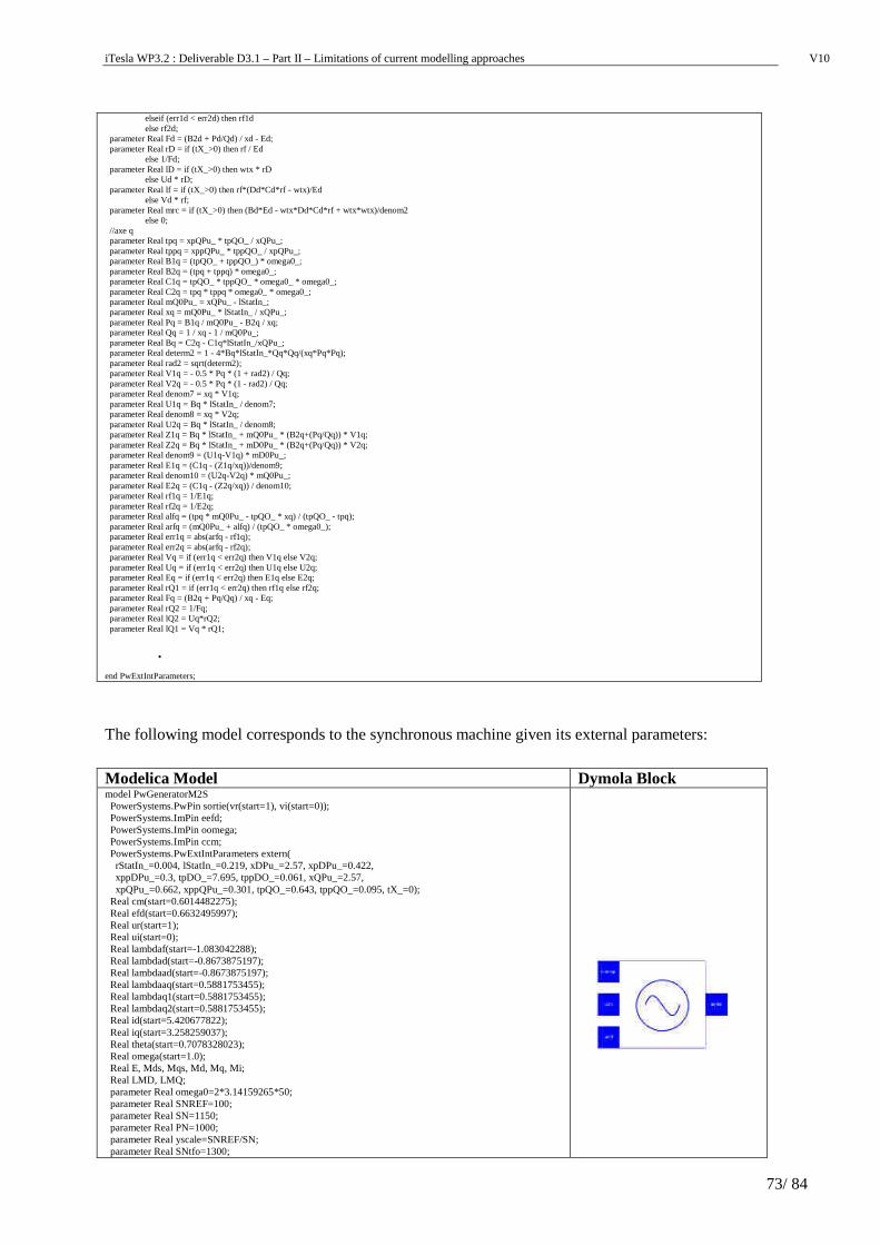
iTesla WP3.2 : Deliverable D3.1 – Part II – Limitations of current modelling approaches V10
73/ 84
elseif (err1d < err2d) then rf1d else rf2d; parameter Real Fd = (B2d + Pd/Qd) / xd - Ed; parameter Real rD = if (tX_>0) then rf / Ed else 1/Fd; parameter Real lD = if (tX_>0) then wtx * rD else Ud * rD; parameter Real lf = if (tX_>0) then rf*(Dd*Cd*rf - wtx)/Ed else Vd * rf; parameter Real mrc = if (tX_>0) then (Bd*Ed - wtx*Dd*Cd*rf + wtx*wtx)/denom2 else 0; //axe q parameter Real tpq = xpQPu_ * tpQO_ / xQPu_; parameter Real tppq = xppQPu_ * tppQO_ / xpQPu_; parameter Real B1q = (tpQO_ + tppQO_) * omega0_; parameter Real B2q = (tpq + tppq) * omega0_; parameter Real C1q = tpQO_ * tppQO_ * omega0_ * omega0_; parameter Real C2q = tpq * tppq * omega0_ * omega0_; parameter Real mQ0Pu_ = xQPu_ - lStatIn_; parameter Real xq = mQ0Pu_ * lStatIn_ / xQPu_; parameter Real Pq = B1q / mQ0Pu_ - B2q / xq; parameter Real Qq = 1 / xq - 1 / mQ0Pu_; parameter Real Bq = C2q - C1q*lStatIn_/xQPu_; parameter Real determ2 = 1 - 4*Bq*lStatIn_*Qq*Qq/(xq*Pq*Pq); parameter Real rad2 = sqrt(determ2); parameter Real V1q = - 0.5 * Pq * (1 + rad2) / Qq; parameter Real V2q = - 0.5 * Pq * (1 - rad2) / Qq; parameter Real denom7 = xq * V1q; parameter Real U1q = Bq * lStatIn_ / denom7; parameter Real denom8 = xq * V2q; parameter Real U2q = Bq * lStatIn_ / denom8; parameter Real Z1q = Bq * lStatIn_ + mQ0Pu_ * (B2q+(Pq/Qq)) * V1q; parameter Real Z2q = Bq * lStatIn_ + mD0Pu_ * (B2q+(Pq/Qq)) * V2q; parameter Real denom9 = (U1q-V1q) * mD0Pu_; parameter Real E1q = (C1q - (Z1q/xq))/denom9; parameter Real denom10 = (U2q-V2q) * mQ0Pu_; parameter Real E2q = (C1q - (Z2q/xq)) / denom10; parameter Real rf1q = 1/E1q; parameter Real rf2q = 1/E2q; parameter Real alfq = (tpq * mQ0Pu_ - tpQO_ * xq) / (tpQO_ - tpq); parameter Real arfq = (mQ0Pu_ + alfq) / (tpQO_ * omega0_); parameter Real err1q = abs(arfq - rf1q); parameter Real err2q = abs(arfq - rf2q); parameter Real Vq = if (err1q < err2q) then V1q else V2q; parameter Real Uq = if (err1q < err2q) then U1q else U2q; parameter Real Eq = if (err1q < err2q) then E1q else E2q; parameter Real rQ1 = if (err1q < err2q) then rf1q else rf2q; parameter Real Fq = (B2q + Pq/Qq) / xq - Eq; parameter Real rQ2 = 1/Fq; parameter Real lQ2 = Uq*rQ2; parameter Real lQ1 = Vq * rQ1;
•
end PwExtIntParameters; The following model corresponds to the synchronous machine given its external parameters: Modelica Model Dymola Block model PwGeneratorM2S PowerSystems.PwPin sortie(vr(start=1), vi(start=0)); PowerSystems.ImPin eefd; PowerSystems.ImPin oomega; PowerSystems.ImPin ccm; PowerSystems.PwExtIntParameters extern( rStatIn_=0.004, lStatIn_=0.219, xDPu_=2.57, xpDPu_=0.422, xppDPu_=0.3, tpDO_=7.695, tppDO_=0.061, xQPu_=2.57, xpQPu_=0.662, xppQPu_=0.301, tpQO_=0.643, tppQO_=0.095, tX_=0); Real cm(start=0.6014482275); Real efd(start=0.6632495997); Real ur(start=1); Real ui(start=0); Real lambdaf(start=-1.083042288); Real lambdad(start=-0.8673875197); Real lambdaad(start=-0.8673875197); Real lambdaaq(start=0.5881753455); Real lambdaq1(start=0.5881753455); Real lambdaq2(start=0.5881753455); Real id(start=5.420677822); Real iq(start=3.258259037); Real theta(start=0.7078328023); Real omega(start=1.0); Real E, Mds, Mqs, Md, Mq, Mi; Real LMD, LMQ; parameter Real omega0=2*3.14159265*50; parameter Real SNREF=100; parameter Real SN=1150; parameter Real PN=1000; parameter Real yscale=SNREF/SN; parameter Real SNtfo=1300;
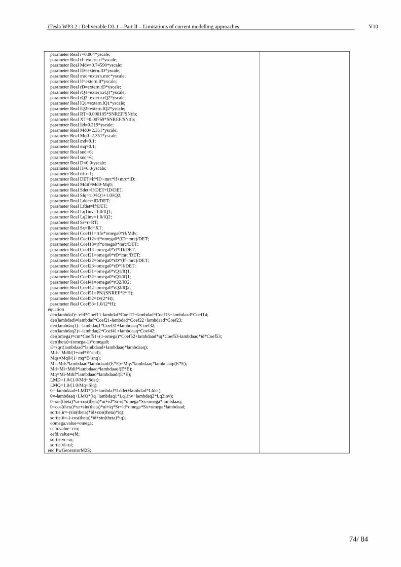
iTesla WP3.2 : Deliverable D3.1 – Part II – Limitations of current modelling approaches V10
74/ 84
parameter Real r=0.004*yscale; parameter Real rf=extern.rf*yscale; parameter Real Mdv=0.74590*yscale; parameter Real lD=extern.lD*yscale; parameter Real mrc=extern.mrc*yscale; parameter Real lf=extern.lf*yscale; parameter Real rD=extern.rD*yscale; parameter Real rQ1=extern.rQ1*yscale; parameter Real rQ2=extern.rQ2*yscale; parameter Real lQ1=extern.lQ1*yscale; parameter Real lQ2=extern.lQ2*yscale; parameter Real RT=0.000185*SNREF/SNtfo; parameter Real XT=0.00769*SNREF/SNtfo; parameter Real lld=0.219*yscale; parameter Real Md0=2.351*yscale; parameter Real Mq0=2.351*yscale; parameter Real md=0.1; parameter Real mq=0.1; parameter Real snd=6; parameter Real snq=6; parameter Real D=0.0/yscale; parameter Real H=6.3/yscale; parameter Real rtfo=1; parameter Real DET=lf*lD+mrc*lf+mrc*lD; parameter Real Mdif=Md0-Mq0; parameter Real Sdet=lf/DET+lD/DET; parameter Real Slq=1.0/lQ1+1.0/lQ2; parameter Real Lddet=lD/DET; parameter Real Lfdet=lf/DET; parameter Real Lq1inv=1.0/lQ1; parameter Real Lq2inv=1.0/lQ2; parameter Real Sr=r+RT; parameter Real Sx=lld+XT; parameter Real Coef11=rtfo*omega0*rf/Mdv; parameter Real Coef12=rf*omega0*(lD+mrc)/DET; parameter Real Coef13=rf*omega0*mrc/DET; parameter Real Coef14=omega0*rf*lD/DET; parameter Real Coef21=omega0*rD*mrc/DET; parameter Real Coef22=omega0*rD*(lf+mrc)/DET; parameter Real Coef23=omega0*rD*lf/DET; parameter Real Coef31=omega0*rQ1/lQ1; parameter Real Coef32=omega0*rQ1/lQ1; parameter Real Coef41=omega0*rQ2/lQ2; parameter Real Coef42=omega0*rQ2/lQ2; parameter Real Coef51=PN/(SNREF*2*H); parameter Real Coef52=D/(2*H); parameter Real Coef53=1.0/(2*H); equation der(lambdaf)=-efd*Coef11-lambdaf*Coef12+lambdad*Coef13+lambdaad*Coef14; der(lambdad)=lambdaf*Coef21-lambdad*Coef22+lambdaad*Coef23; der(lambdaq1)=-lambdaq1*Coef31+lambdaaq*Coef32; der(lambdaq2)=-lambdaq2*Coef41+lambdaaq*Coef42; der(omega)=cm*Coef51+(1-omega)*Coef52+lambdaad*iq*Coef53-lambdaaq*id*Coef53; der(theta)=(omega-1)*omega0; E=sqrt(lambdaad*lambdaad+lambdaaq*lambdaaq); Mds=Md0/(1+md*E^snd); Mqs=Mq0/(1+mq*E^snq); Mi=Mds*lambdaad*lambdaad/(E*E)+Mqs*lambdaaq*lambdaaq/(E*E); Md=Mi+Mdif*lambdaaq*lambdaaq/(E*E); Mq=Mi-Mdif*lambdaad*lambdaad/(E*E); LMD=1.0/(1.0/Md+Sdet); LMQ=1.0/(1.0/Mq+Slq); 0=-lambdaad+LMD*(id+lambdaf*Lddet+lambdad*Lfdet); 0=-lambdaaq+LMQ*(iq+lambdaq1*Lq1inv+lambdaq2*Lq2inv); 0=sin(theta)*ur-cos(theta)*ui+id*Sr-iq*omega*Sx-omega*lambdaaq; 0=cos(theta)*ur+sin(theta)*ui+iq*Sr+id*omega*Sx+omega*lambdaad; sortie.ir=-(sin(theta)*id+cos(theta)*iq); sortie.ii=-(-cos(theta)*id+sin(theta)*iq); oomega.value=omega; ccm.value=cm; eefd.value=efd; sortie.vr=ur; sortie.vi=ui; end PwGeneratorM2S;
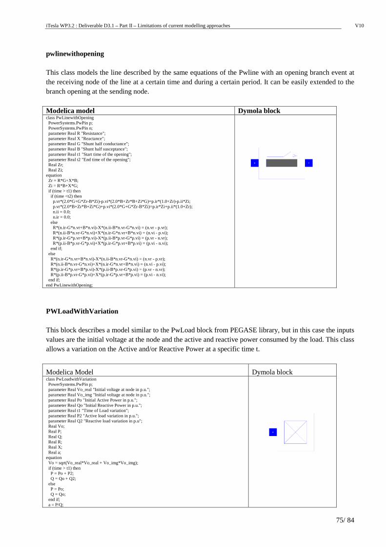
iTesla WP3.2 : Deliverable D3.1 – Part II – Limitations of current modelling approaches V10
75/ 84
pwlinewithopening This class models the line described by the same equations of the Pwline with an opening branch event at the receiving node of the line at a certain time and during a certain period. It can be easily extended to the branch opening at the sending node. Modelica model Dymola block class PwLinewithOpening PowerSystems.PwPin p; PowerSystems.PwPin n; parameter Real R "Resistance"; parameter Real X "Reactance"; parameter Real G "Shunt half conductance"; parameter Real B "Shunt half susceptance"; parameter Real t1 "Start time of the opening"; parameter Real t2 "End time of the opening"; Real Zr; Real Zi; equation Zr = R*G+X*B; Zi = R*B+X*G; if (time > t1) then if (time <t2) then p.vr*(2.0*G+G*Zr-B*Zi)-p.vi*(2.0*B+Zr*B+Zi*G) =p.ir*(1.0+Zr)-p.ii*Zi; p.vr*(2.0*B+Zr*B+Zi*G)+p.vi*(2.0*G+G*Zr-B*Zi) =p.ir*Zi+p.ii*(1.0+Zr); n.ii = 0.0; n.ir = 0.0; else R*(n.ir-G*n.vr+B*n.vi)-X*(n.ii-B*n.vr-G*n.vi) = (n.vr - p.vr); R*(n.ii-B*n.vr-G*n.vi)+X*(n.ir-G*n.vr+B*n.vi) = (n.vi - p.vi); R*(p.ir-G*p.vr+B*p.vi)-X*(p.ii-B*p.vr-G*p.vi) = (p.vr - n.vr); R*(p.ii-B*p.vr-G*p.vi)+X*(p.ir-G*p.vr+B*p.vi) = (p.vi - n.vi); end if; else R*(n.ir-G*n.vr+B*n.vi)-X*(n.ii-B*n.vr-G*n.vi) = (n.vr - p.vr); R*(n.ii-B*n.vr-G*n.vi)+X*(n.ir-G*n.vr+B*n.vi) = (n.vi - p.vi); R*(p.ir-G*p.vr+B*p.vi)-X*(p.ii-B*p.vr-G*p.vi) = (p.vr - n.vr); R*(p.ii-B*p.vr-G*p.vi)+X*(p.ir-G*p.vr+B*p.vi) = (p.vi - n.vi); end if; end PwLinewithOpening;
PWLoadWithVariation This block describes a model similar to the PwLoad block from PEGASE library, but in this case the inputs values are the initial voltage at the node and the active and reactive power consumed by the load. This class allows a variation on the Active and/or Reactive Power at a specific time t.
Modelica Model Dymola block class PwLoadwithVariation PowerSystems.PwPin p; parameter Real Vo_real "Initial voltage at node in p.u."; parameter Real Vo_img "Initial voltage at node in p.u."; parameter Real Po "Initial Active Power in p.u."; parameter Real Qo "Initial Reactive Power in p.u."; parameter Real t1 "Time of Load variation"; parameter Real P2 "Active load variation in p.u."; parameter Real Q2 "Reactive load variation in p.u"; Real Vo; Real P; Real Q; Real R; Real X; Real a; equation Vo = sqrt(Vo_real*Vo_real + Vo_img*Vo_img); if (time > t1) then P = Po + P2; Q = Qo + Q2; else P = Po; Q = Qo; end if; a = P/Q;
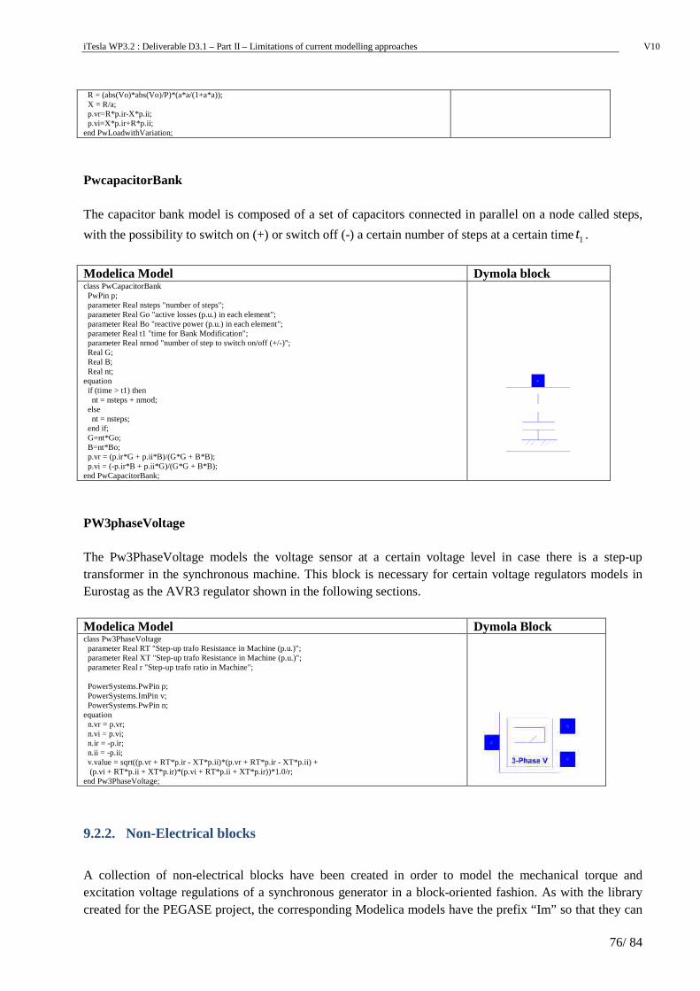
iTesla WP3.2 : Deliverable D3.1 – Part II – Limitations of current modelling approaches V10
76/ 84
R = (abs(Vo)*abs(Vo)/P)*(a*a/(1+a*a)); X = R/a; p.vr=R*p.ir-X*p.ii; p.vi=X*p.ir+R*p.ii; end PwLoadwithVariation;
PwcapacitorBank The capacitor bank model is composed of a set of capacitors connected in parallel on a node called steps,
with the possibility to switch on (+) or switch off (-) a certain number of steps at a certain time1t .
Modelica Model Dymola block class PwCapacitorBank PwPin p; parameter Real nsteps "number of steps"; parameter Real Go "active losses (p.u.) in each element"; parameter Real Bo "reactive power (p.u.) in each element"; parameter Real t1 "time for Bank Modification"; parameter Real nmod "number of step to switch on/off (+/-)"; Real G; Real B; Real nt; equation if (time > t1) then nt = nsteps + nmod; else nt = nsteps; end if; G=nt*Go; B=nt*Bo; p.vr = (p.ir*G + p.ii*B)/(G*G + B*B); p.vi = (-p.ir*B + p.ii*G)/(G*G + B*B); end PwCapacitorBank;
PW3phaseVoltage The Pw3PhaseVoltage models the voltage sensor at a certain voltage level in case there is a step-up transformer in the synchronous machine. This block is necessary for certain voltage regulators models in Eurostag as the AVR3 regulator shown in the following sections. Modelica Model Dymola Block class Pw3PhaseVoltage parameter Real RT "Step-up trafo Resistance in Machine (p.u.)"; parameter Real XT "Step-up trafo Resistance in Machine (p.u.)"; parameter Real r "Step-up trafo ratio in Machine"; PowerSystems.PwPin p; PowerSystems.ImPin v; PowerSystems.PwPin n; equation n.vr = p.vr; n.vi = p.vi; n.ir = -p.ir; n.ii = -p.ii; v.value = sqrt((p.vr + RT*p.ir - XT*p.ii)*(p.vr + RT*p.ir - XT*p.ii) + (p.vi + RT*p.ii + XT*p.ir)*(p.vi + RT*p.ii + XT*p.ir))*1.0/r; end Pw3PhaseVoltage;
9.2.2. Non-Electrical blocks
A collection of non-electrical blocks have been created in order to model the mechanical torque and excitation voltage regulations of a synchronous generator in a block-oriented fashion. As with the library created for the PEGASE project, the corresponding Modelica models have the prefix “Im” so that they can
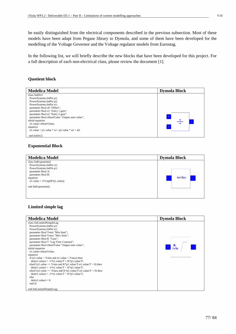
iTesla WP3.2 : Deliverable D3.1 – Part II – Limitations of current modelling approaches V10
77/ 84
be easily distinguished from the electrical components described in the previous subsection. Most of these models have been adapt from Pegase library to Dymola, and some of them have been developed for the modelling of the Voltage Governor and the Voltage regulator models from Eurostag. In the following list, we will briefly describe the new blocks that have been developed for this project. For a full description of each non-electrical class, please review the document [1]. Quotient block Modelica Model Dymola Block class ImDiv2 PowerSystems.ImPin p1; PowerSystems.ImPin p2; PowerSystems.ImPin n1; parameter Real a0 "Offset"; parameter Real a1 "Entry 1 gain"; parameter Real a2 "Entry 2 gain"; parameter Real nStartValue "Output start value"; initial equation n1.value=nStartValue; equation n1.value = p1.value * a1 / p2.value * a2 + a0;
end ImDiv2;
Exponential Block Modelica Model Dymola Block class ImExponential PowerSystems.ImPin n1; PowerSystems.ImPin p1; parameter Real A; parameter Real B; equation n1.value = A*exp(B*p1.value);
end ImExponential;
Limited simple lag Modelica Model Dymola Block class ImLimitedSimpleLag PowerSystems.ImPin p1; PowerSystems.ImPin n1; parameter Real Ymin "Min limit"; parameter Real Ymax "Max limit"; parameter Real K "Gain"; parameter Real T "Lag Time Constant"; parameter Real nStartValue "Output start value"; initial equation n1.value=nStartValue; equation if (n1.value > Ymin and n1.value < Ymax) then der(n1.value) = -1*n1.value/T + K*p1.value/T; elseif (n1.value <= Ymin and K*p1.value/T-n1.value/T > 0) then der(n1.value) = -1*n1.value/T + K*p1.value/T; elseif (n1.value >= Ymax and K*p1.value/T-n1.value/T < 0) then der(n1.value) = -1*n1.value/T + K*p1.value/T; else der(n1.value) = 0; end if;
end ImLimitedSimpleLag;
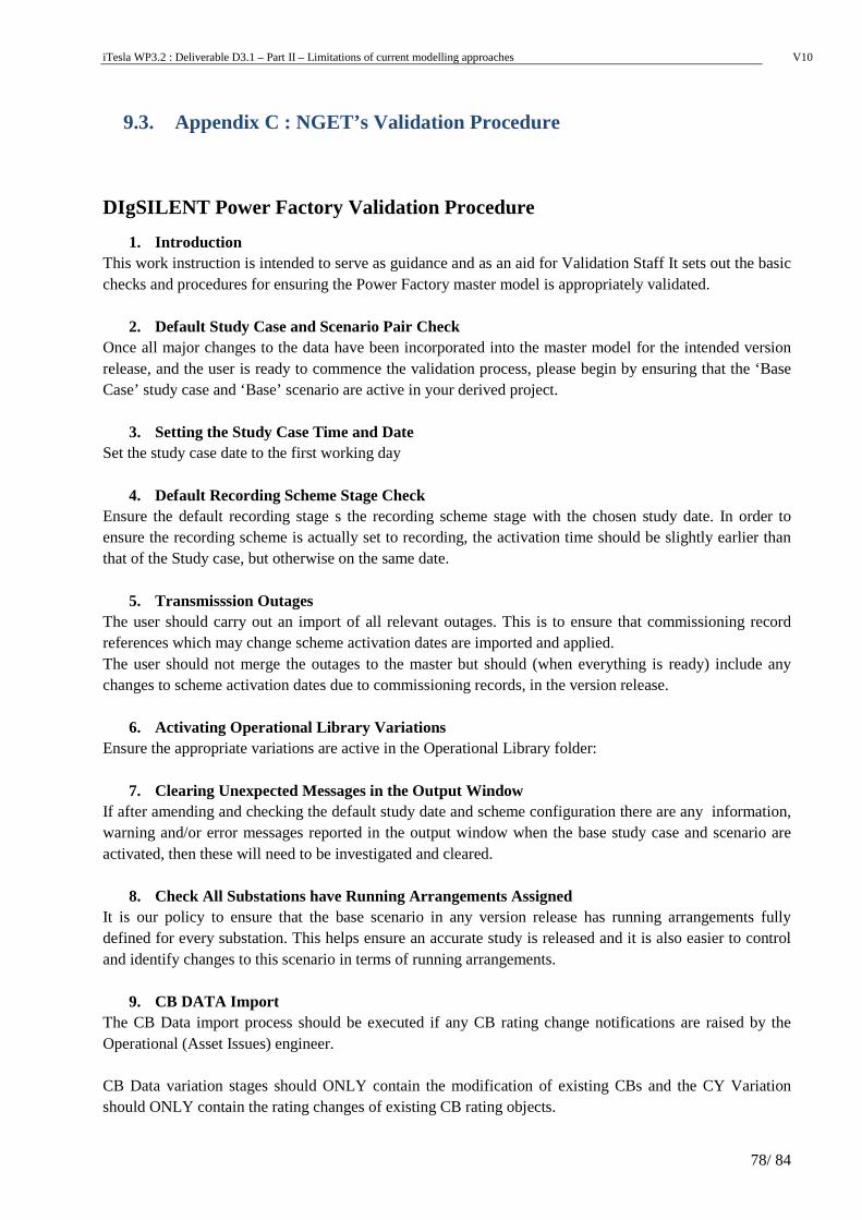
iTesla WP3.2 : Deliverable D3.1 – Part II – Limitations of current modelling approaches V10
78/ 84
9.3. Appendix C : NGET’s Validation Procedure
DIgSILENT Power Factory Validation Procedure
1. Introduction This work instruction is intended to serve as guidance and as an aid for Validation Staff It sets out the basic checks and procedures for ensuring the Power Factory master model is appropriately validated.
2. Default Study Case and Scenario Pair Check Once all major changes to the data have been incorporated into the master model for the intended version release, and the user is ready to commence the validation process, please begin by ensuring that the ‘Base Case’ study case and ‘Base’ scenario are active in your derived project.
3. Setting the Study Case Time and Date Set the study case date to the first working day
4. Default Recording Scheme Stage Check Ensure the default recording stage s the recording scheme stage with the chosen study date. In order to ensure the recording scheme is actually set to recording, the activation time should be slightly earlier than that of the Study case, but otherwise on the same date.
5. Transmisssion Outages The user should carry out an import of all relevant outages. This is to ensure that commissioning record references which may change scheme activation dates are imported and applied. The user should not merge the outages to the master but should (when everything is ready) include any changes to scheme activation dates due to commissioning records, in the version release.
6. Activating Operational Library Variations Ensure the appropriate variations are active in the Operational Library folder:
7. Clearing Unexpected Messages in the Output Window If after amending and checking the default study date and scheme configuration there are any information, warning and/or error messages reported in the output window when the base study case and scenario are activated, then these will need to be investigated and cleared.
8. Check All Substations have Running Arrangements Assigned It is our policy to ensure that the base scenario in any version release has running arrangements fully defined for every substation. This helps ensure an accurate study is released and it is also easier to control and identify changes to this scenario in terms of running arrangements.
9. CB DATA Import The CB Data import process should be executed if any CB rating change notifications are raised by the Operational (Asset Issues) engineer. CB Data variation stages should ONLY contain the modification of existing CBs and the CY Variation should ONLY contain the rating changes of existing CB rating objects.
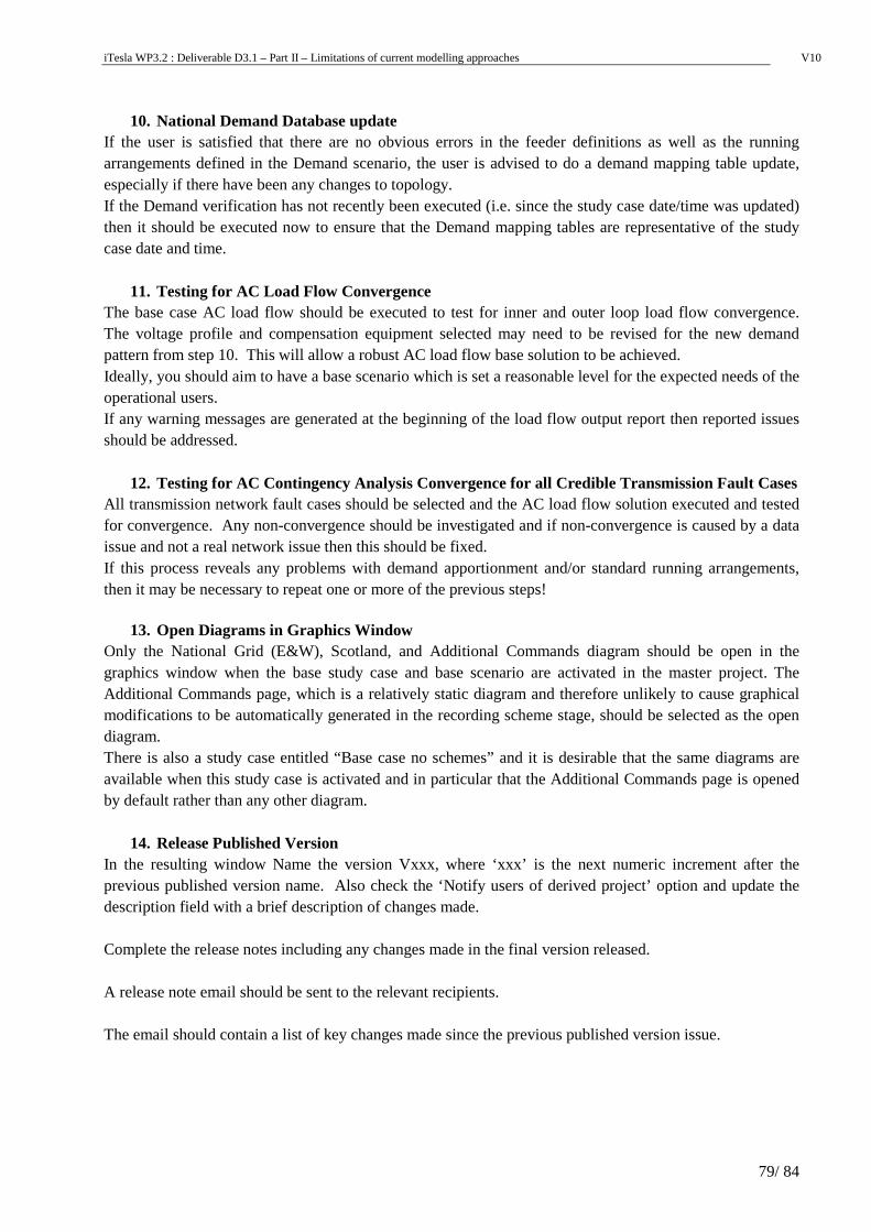
iTesla WP3.2 : Deliverable D3.1 – Part II – Limitations of current modelling approaches V10
79/ 84
10. National Demand Database update If the user is satisfied that there are no obvious errors in the feeder definitions as well as the running arrangements defined in the Demand scenario, the user is advised to do a demand mapping table update, especially if there have been any changes to topology. If the Demand verification has not recently been executed (i.e. since the study case date/time was updated) then it should be executed now to ensure that the Demand mapping tables are representative of the study case date and time.
11. Testing for AC Load Flow Convergence The base case AC load flow should be executed to test for inner and outer loop load flow convergence. The voltage profile and compensation equipment selected may need to be revised for the new demand pattern from step 10. This will allow a robust AC load flow base solution to be achieved. Ideally, you should aim to have a base scenario which is set a reasonable level for the expected needs of the operational users. If any warning messages are generated at the beginning of the load flow output report then reported issues should be addressed.
12. Testing for AC Contingency Analysis Convergence for all Credible Transmission Fault Cases All transmission network fault cases should be selected and the AC load flow solution executed and tested for convergence. Any non-convergence should be investigated and if non-convergence is caused by a data issue and not a real network issue then this should be fixed. If this process reveals any problems with demand apportionment and/or standard running arrangements, then it may be necessary to repeat one or more of the previous steps!
13. Open Diagrams in Graphics Window Only the National Grid (E&W), Scotland, and Additional Commands diagram should be open in the graphics window when the base study case and base scenario are activated in the master project. The Additional Commands page, which is a relatively static diagram and therefore unlikely to cause graphical modifications to be automatically generated in the recording scheme stage, should be selected as the open diagram. There is also a study case entitled “Base case no schemes” and it is desirable that the same diagrams are available when this study case is activated and in particular that the Additional Commands page is opened by default rather than any other diagram.
14. Release Published Version In the resulting window Name the version Vxxx, where ‘xxx’ is the next numeric increment after the previous published version name. Also check the ‘Notify users of derived project’ option and update the description field with a brief description of changes made. Complete the release notes including any changes made in the final version released. A release note email should be sent to the relevant recipients. The email should contain a list of key changes made since the previous published version issue.

iTesla WP3.2 : Deliverable D3.1 – Part II – Limitations of current modelling approaches
Limitations of current modelling approaches
V10
80/ 84
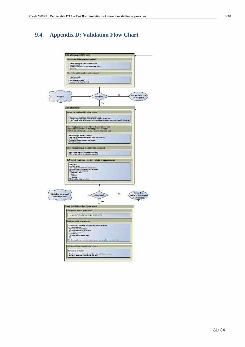
iTesla WP3.2 : Deliverable D3.1 – Part II – Limitations of current modelling approaches V10
81/ 84
9.4. Appendix D: Validation Flow Chart
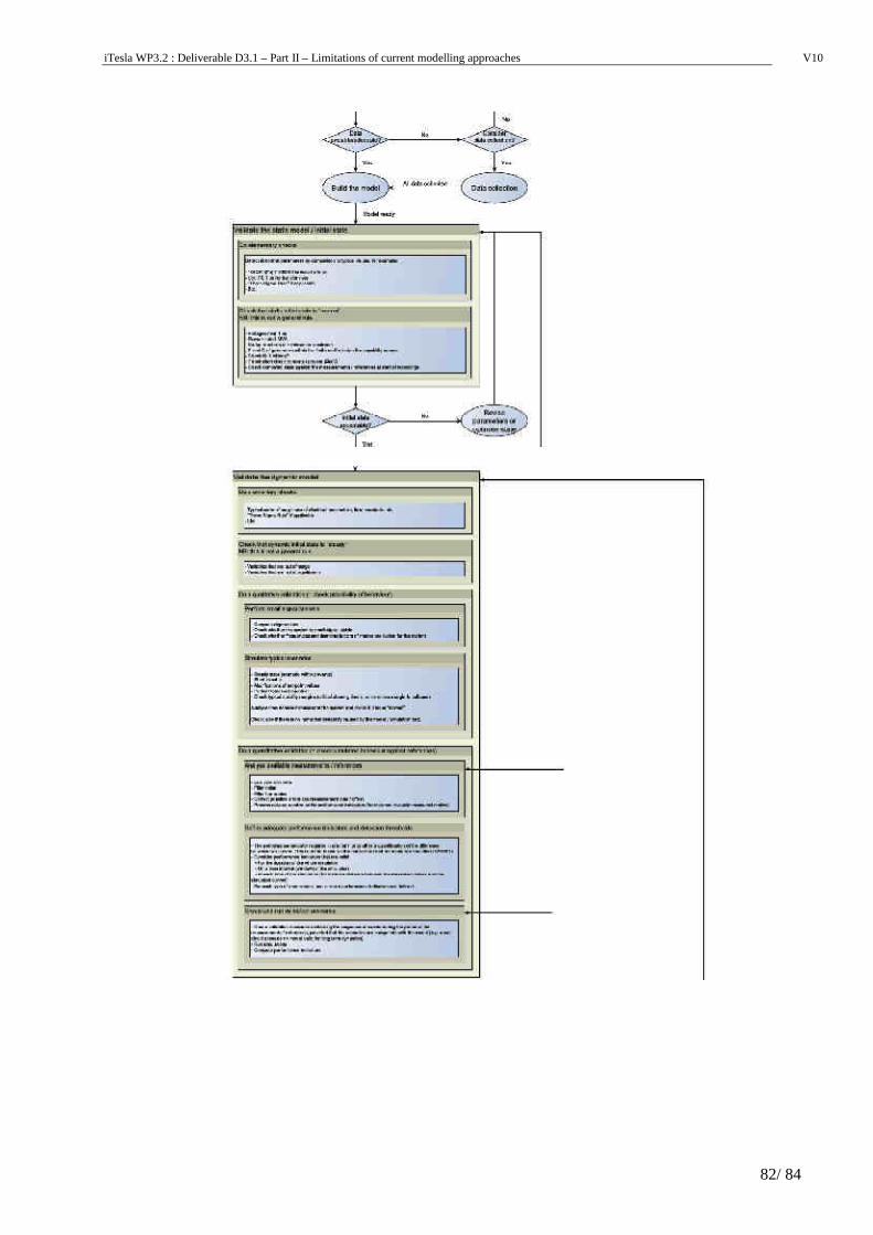
iTesla WP3.2 : Deliverable D3.1 – Part II – Limitations of current modelling approaches V10
82/ 84
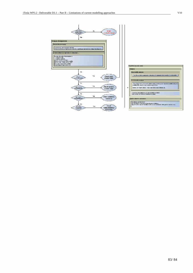
iTesla WP3.2 : Deliverable D3.1 – Part II – Limitations of current modelling approaches V10
83/ 84


![D3.1 Modularreasoningforsystemvalidation andverification€¦ · D3.1-Modularreasoningforsystemvalidationandverification Chapter2 Frama-Ctoolbox 2.1 Frama-Ckernel Frama-C[17]isaplatformdedicatedtotheanalysisofCprograms](https://img.pdfslide.us/doc/110x75/605aeaff01f74a5add78b68c/d31-modularreasoningforsystemvalidation-andverification-d31-modularreasoningforsystemvalidationandverification.jpg)