Embed Size (px)
Citation preview
1
Project Deliverable
Grant Agreement number 308952
Project acronym OMSOP
Project title OPTIMISED MICROTURBINE SOLAR POWER SYSTEM
Funding Scheme FP7-ENERGY.2012.2.5.1:RESEARCH, DEVELOPMENT AND TESTING OF SOLAR DISH SYSTEMS
Work Package WP1 – SYSTEM COMPONENT DEVELOPMENT
Deliverable number - title D1.5 OPTIMIZED DISH DESIGN
Lead Beneficiary INNOVA
Dissemination level PU
Delivery month JANUARY 2013
Name, title and organisation of the scientific representative of the project's coordinator
Prof. Abdulnaser Sayma
Professor of Energy Engineering
City University London
Tel: +44 (0)20 7040 8277
E-mail: [email protected]
Project website address: www.omsop.eu
Authors: Tommaso Crescenzi (ENEA), Michela Lanchi ( ENEA), Valeria Russo (ENEA), Adio
Miliozzi (ENEA), Marco Montecchi (ENEA), Enzo Pasto relli (Innova), Alessandro Mariani (Innova)
2
Contents
Introduction ........................................................................................................................... 3
Stand-alone dish array: a feasibility analysis ......................................................................... 4
Dish shape optimization and performance analysis ............................................................... 8
Dish shape optimization ..................................................................................................... 8
Geometrical aspects ............................................................................................................ 8 Optics of the parabolic dish concentrator ........................................................................... 9 Efficiency evaluation ......................................................................................................... 16 Application of the “ray tracing” method .......................................................................... 21 Conclusions ....................................................................................................................... 28
Performance analysis .......................................................................................................29
Dimensions of the Innova PDC ......................................................................................... 29 Focal plane flux distribution using a ray-tracing method ................................................. 30 Efficiency evaluation ......................................................................................................... 32 Conclusions ....................................................................................................................... 38
SIMUL-DISH: a portable ray tracing software for analytical dish simulation ..........................40
Software description .........................................................................................................40
Comparison between single and daisy-arrangement of dishes .........................................44
Simulation according to the latest OMSoP project outlining ..............................................48
Wind loads analysis ..............................................................................................................50
Codes and Standards .......................................................................................................50
Definition of the wind actions ............................................................................................50
Aerodynamic coefficients: CNR-DT207/2008 ....................................................................51
Aerodynamic coefficients: Wind tunnel experimental tests ................................................54
Aerodynamic coefficients: methods comparison ...............................................................60
Characterization of the ENEA Casaccia site .....................................................................63
Evaluation of the peak forces and moments .....................................................................64
Conclusions ......................................................................................................................64
Supporting structure .............................................................................................................65
Tracking system specifications .............................................................................................69
References ...........................................................................................................................71
3
Introduction The main objective of the project is to develop and demonstrate advanced technical solutions for concentrated solar power systems (CSP) coupled to micro-gas turbine (MGT) to produce electricity in the range of 3-10 kW. The system is destined to fulfil energy needs for domestic and small commercial applications. The primary technical challenge is to enable the production of small scale cost effective, efficient and reliable units. The parabolic dish concentrator technology, in particular, has to be improved in terms of concentration ratio increase and weight reduction. With this regard, the partners have considered different design solutions with the aim of increasing the dish performances maintaining a light and handy structure. Different dish configurations have been analysed, with a particular focus on two possible options: multi-dish arrangement, consisting of a structure composed of several dishes, or single dish configuration. In particular two possible configurations have been considered for the multi-dish arrangement: the “array” system, described and analysed in the paragraph “Stan-alone dish array: a feasibility analysis”, and the “daisy” structure, described and evaluated in the paragraph “SIMUL-DISH: a portable ray tracing software for analytical dish simulation”. The selected dish arrangement has been successively tailored to the MGT-receiver requirements. In particular the solar collector has been optimized in terms of shape and materials for achieving the target concentration factor and turbine inlet temperature (~800°C). The optimization analysis and the dish performance evaluation have been reported in the paragraph “Dish shape optimization and performance analysis”. Once defined the geometrical specifications of the dish, which will be realized and tested at Casaccia site, a wind load analysis has been carried out with the aim of evaluating the wind loads acting in realistic environmental conditions. The theoretical study and the results have been reported in the paragraph “Wind loads analysis”. On the base of the dish geometrical specifications and calculated mechanical loads the supporting structure of the dish prototype has been defined along with the tracking system. Their description is reported in the paragraphs “Supporting structure” and “Tracking system specification”.
4
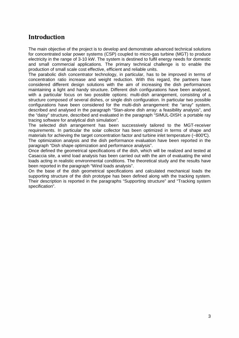
Stand-alone dish array: a feasibility analysis (Tommaso Crescenzi, Michela Lanchi, Valeria Russo (ENEA) In the frame of the Task1.2 “Dish arrangement design and optimization”, different dish configurations have been analysed, with a particular focus on the multi-dish arrangement, intended as a system composed of several dishes, with the aim of increasing the concentration factor and the turbine inlet temperature maintaining light and handy structures. In particular, two options have been investigated: the “daisy arrangement”, consisting in a concentrator structure composed of several dishes (4-6), and the “stand-alone dish array”, consisting in an array of separate dishes, each connected to a separate receiver. The analysis of the latter configuration is the object of the present paragraph. The theoretical analysis has been performed assuming that all the dishes composing the array have the same concentration factor and that all the receivers are connected each other to provide the required thermal energy to a single Micro Gas Turbine (MGT), as shown in Figure 1. As a first consideration, it is worth noticing that this option, with respect to the single dish configuration, implies a more expensive concentration system and a more extensive use of land. Furthermore this layout leads to an efficiency reduction because of the relevant extension of the piping system required to connect the dish array unit to the MGT system. Indeed the piping network is composed of a principal header and several secondary lines (see Fig. 1) with inevitable thermal and mechanical energy losses, and consequently an overall efficiency reduction.
Figure 1 – Scheme of the stand-alone dish array concept
In order to compensate these losses and to maintain the same operation conditions at the inlet of the MGT it would be necessary to increase the outlet temperature of the receivers and the outlet pressure of the air compressor. With the aim of evaluating the thermal and the mechanical energy losses related to the dish array option, a comparison between a single dish lay-out (60 m2 of reflecting surface and 9 m of diameter) and a dish array configuration composed of 6 dishes (each characterized by 12 m2 of reflecting surface and 4 m of diameter) has been carried out in terms of thermal performance.
5
The thermal efficiency of the dish-receiver system has been assumed equal to 50%, considering the optical efficiency of the dishes equal to 72% and the thermal efficiency of the receivers equal to 70%. Furthermore the concentration factor has been assumed to be constant in the two configurations, meaning that the receiver window in the dish array option is smaller than the single dish arrangement. With regard to the direct normal irradiation (DNI), a value of 900 W/m2 has been assumed. As for the MGT, represented in Figure 2, the following operative conditions have been assumed:
• Compressor outlet pressure (kPa) 320 • Turbine inlet temperature (°C) 750 • Air mass flow (kg/s) 0.1 • Compressor isoentropic efficiency (%) 76 • Turbine isoentropic efficiency (%) 80 • Recuperator efficiency (%) 90
The heat and mass balance calculation has been performed through the use of the GateCycle code, a commercial heat balance software for power plant simulation.
6
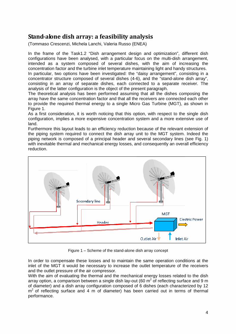
Figure 2 – Comparison between the single dish option and the stand-alone dish array configuration: process simulation through GateCycle code.
SINGLE DISH SYSTEM Since the dish reflecting surface is 60 m2, and the dish-receiver system efficiency is 50%, the solar power collected is 54 kWt, while the power available at the MGT inlet is about 27 kWt. Considering the turbo alternator friction and the compression work, the turbine net electrical power is 7.7 kWe, with a solar to electricity conversion efficiency of about 14%. STAND-ALONE DISH ARRAY SYSTEM As above mentioned the MGT unit is located outside the solar field, and connected to each receiver through a network of piping for the collection and distribution of the air flow. In analogy to what has been assumed for the single-dish system, the power available at each receiver window is 6.5 kWt. (54*0.72/6 kWt) Regarding the piping system, it has been hypothesized that it is 30 m long and properly insulated. Therefore, assuming a linear thermal loss of about 150 W/m, the total power lost from the piping system can be estimated as 4.5 kW. Regarding the mechanical losses it has been assumed that the piping pressure drops represent a fixed percentage of the compressor outlet pressure (5% of 320 kPa). On the base of these energy losses values, the heat and mass balance along the piping has been performed using the GateCycle simulation code. In particular the component “Duct” has been selected to simulate the behavior of the piping. The calculated temperature and pressure at the turbine inlet are 710°C and 287 kPa, respectively, while in the single-dish option they are 750°C and 320 kPa, respectively. In this case the power available at the MGT

7
inlet is 22.5 kWt, while the net turbine electrical power is 5.1 kWe, with a solar to electricity conversion efficiency of 9.4%. Therefore the thermal and mechanical energy losses have led to a reduction of about 34% of the net turbine electrical power with respect to the single dish case.
CONCLUSIONS From the previous analysis it has clearly emerged that the use of the dish array configuration in place of the single dish option would significantly reduce the solar to electrical conversion efficiency of the system, increasing, at the same time, the investment costs. Furthermore, with the aim of achieving the same operative conditions for the MGT unit (temperature and pressure) it would be necessary to increase the dishes surface and the pressure ratio of the compressor. The single dish option which allows the physical integration between the receiver and the MGT unit is therefore more efficient and less expensive. The adoption of the stand-alone dish array option is desirable only in view of a modular electricity production, with each dish equipped with its own receiver and MGT.
8
Dish shape optimization and performance analysis (Adio Miliozzi (ENEA))
Dish shape optimization
As already mentioned in the introduction, the parabolic dish collector (PDC) system has to be coupled with a micro-gas-turbine (MGT) with electrical power (Pe) between 3 and 10 kWe. The micro-gas-turbine should run with a receiver temperature of about 800-1000°C. Assuming a maximum solar radiation (I) of about 800 W/m2, a maximum global efficiency of about 25% (ηtot), and an utilization factor of the total area, fused, of about 90%, we should get:
• A useful receiving surface: Snet = Pe/ (ηtot I) = 15 - 50 m2 ; • A total receiving surface: Stot = Snet / fused = 16.7 - 55.6 m2 ; • An aperture diameter of the parabolic dish: D = (4*Stot / π)^0.5 = 4.6 – 8.4 m
Consequently, the following analysis will be focused on parabolic dish concentrators having aperture diameters between 4 and 10 meters , optimized to achieve a cavity receiver temperature of the order of 1000 °C .
Geometrical aspects
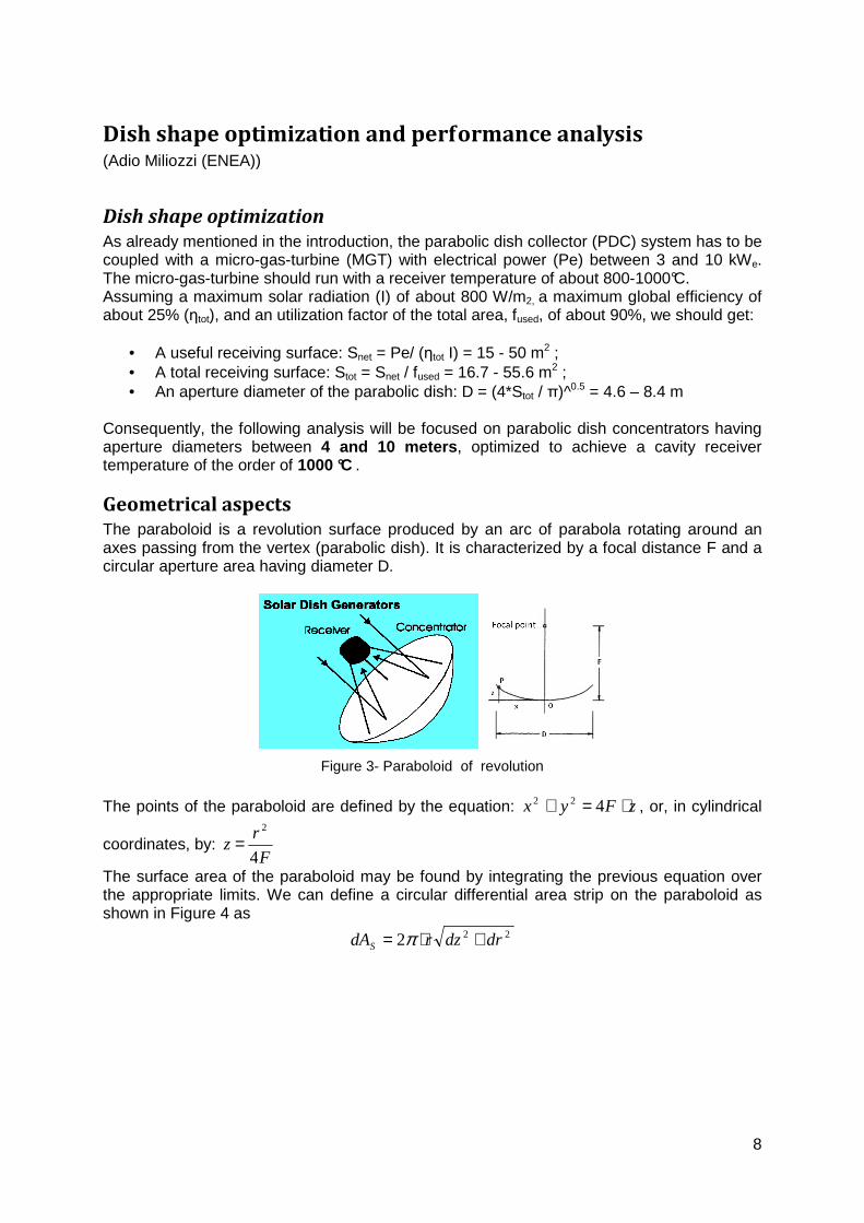
The paraboloid is a revolution surface produced by an arc of parabola rotating around an axes passing from the vertex (parabolic dish). It is characterized by a focal distance F and a circular aperture area having diameter D.
Figure 3- Paraboloid of revolution The points of the paraboloid are defined by the equation: zFyx ⋅=+ 422 , or, in cylindrical
coordinates, by: F
rz
4
2
=
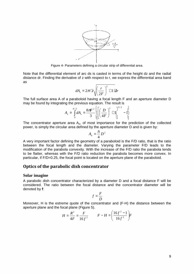
The surface area of the paraboloid may be found by integrating the previous equation over the appropriate limits. We can define a circular differential area strip on the paraboloid as shown in Figure 4 as
222 drdzrdAS +⋅= π
9
Figure 4- Parameters defining a circular strip of differential area.
Note that the differential element of arc ds is casted in terms of the height dz and the radial distance dr. Finding the derivative of z with respect to r, we express the differential area band as
drF
rrdAs ⋅+
⋅= 12
22
π
The full surface area A of a paraboloid having a focal length F and an aperture diameter D may be found by integrating the previous equation. The result is
−
+
== ∫ 1143
82/3222/
0 F
DFdAA
d
ss
π
The concentrator aperture area Aa, of most importance for the prediction of the collected power, is simply the circular area defined by the aperture diameter D and is given by:
2
4DAa
π=
A very important factor defining the geometry of a paraboloid is the F/D ratio, that is the ratio between the focal length and the diameter. Varying the parameter F/D leads to the modification of the parabola convexity. With the increase of the F/D ratio the parabola tends to be flatter, whereas with the F/D ratio reduction the parabola becomes more convex. In particular, if F/D=0.25, the focal point is located on the aperture plane of the paraboloid.
Optics of the parabolic dish concentrator
Solar imagine A parabolic dish concentrator characterized by a diameter D and a focal distance F will be considered. The ratio between the focal distance and the concentrator diameter will be denoted by f:
D
Ff =
Moreover, H is the estreme quote of the concentrator and (F-H) the distance between the aperture plane and the focal plane (Figure 5).
2
2
164 f
F
F
RH ==
Ff
fHF
−=−2
2
16
116
10
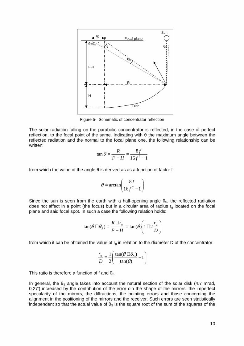
Figure 5- Schematic of concentrator reflection
The solar radiation falling on the parabolic concentrator is reflected, in the case of perfect reflection, to the focal point of the same. Indicating with θ the maximum angle between the reflected radiation and the normal to the focal plane one, the following relationship can be written:
116
8tan
2 −=
−=
f
f
HF
Rθ
from which the value of the angle θ is derived as as a function of factor f:
−=
116
8arctan
2f
fθ
Since the sun is seen from the earth with a half-opening angle θS, the reflected radiation does not affect in a point (the focus) but in a circular area of radius rg located on the focal plane and said focal spot. In such a case the following relation holds:
+=
−+
=+D
r
HF
rR ggS 21)tan()tan( θθθ
from which it can be obtained the value of rg in relation to the diameter D of the concentrator:
−
+= 1
)tan(
)tan(
2
1
θθθ Sg
D
r
This ratio is therefore a function of f and θS. In general, the θS angle takes into account the natural section of the solar disk (4.7 mrad, 0.27°) increased by the contribution of the error o n the shape of the mirrors, the imperfect specularity of the mirrors, the diffractions, the pointing errors and those concerning the alignment in the positioning of the mirrors and the receiver. Such errors are seen statistically independent so that the actual value of θS is the square root of the sum of the squares of the
rg
Dish
θS
F Focal plane
F-H
H
θS
θ θ+θS
R
Sun
11
individual errors. This value θS can be estimated equal to about 7-10 mrad (0.4°-0. 57°) considering also the imperfections of the reflecting surface. The concentration factor C of the focal spot will then have the following expression, function of the ratio between rg and D:
2)/(4
1
DrIC
g
mf =Φ
=
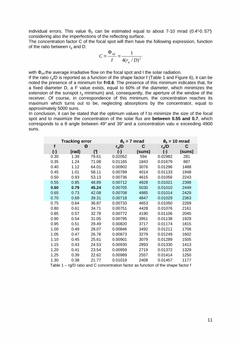
with Φmf the average irradiative flow on the focal spot and I the solar radiation. If the ratio rg/D is reported as a function of the shape factor f (Table 1 and Figure 6), it can be noted the presence of a minimum for f=0.6. The presence of this minimum indicates that, for a fixed diameter D, a F value exists, equal to 60% of the diameter, which minimizes the extension of the sunspot rg minimum) and, consequently, the aperture of the window of the receiver. Of course, in correspondence of this minimum, the concentration reaches its maximum which turns out to be, neglecting absorptions by the concentrator, equal to approximately 5000 suns. In conclusion, it can be stated that the optimum values of f to minimize the size of the focal spot and to maximize the concentration of the solar flux are between 0.55 and 0.7 , which corresponds to a θ angle between 49° and 39° and a concentration valu e exceeding 4900 suns.
Tracking error θS = 7 mrad θS = 10 mrad f Θ rg/D C rg/D C
(-) (rad) (°) (-) (suns ) (-) (suns ) 0.30 1.39 79.61 0.02052 594 0.02982 281 0.35 1.24 71.08 0.01165 1843 0.01679 887 0.40 1.12 64.01 0.00902 3076 0.01296 1488 0.45 1.01 58.11 0.00789 4014 0.01133 1948 0.50 0.93 53.13 0.00736 4615 0.01056 2243 0.55 0.85 48.89 0.00712 4928 0.01021 2398 0.60 0.79 45.24 0.00705 5030 0.01010 2449 0.65 0.73 42.08 0.00708 4985 0.01014 2429 0.70 0.69 39.31 0.00718 4847 0.01029 2363 0.75 0.64 36.87 0.00733 4653 0.01050 2269 0.80 0.61 34.71 0.00751 4428 0.01076 2161 0.85 0.57 32.78 0.00772 4190 0.01106 2045 0.90 0.54 31.05 0.00795 3951 0.01138 1929 0.95 0.51 29.49 0.00820 3717 0.01174 1815 1.00 0.49 28.07 0.00846 3492 0.01211 1706 1.05 0.47 26.78 0.00873 3279 0.01249 1602 1.10 0.45 25.61 0.00901 3079 0.01289 1505 1.15 0.43 24.53 0.00930 2893 0.01330 1413 1.20 0.41 23.54 0.00959 2719 0.01372 1329 1.25 0.39 22.62 0.00989 2557 0.01414 1250 1.30 0.38 21.77 0.01019 2408 0.01457 1177 Table 1 – rg/D ratio and C concentration factor as function of the shape factor f
12
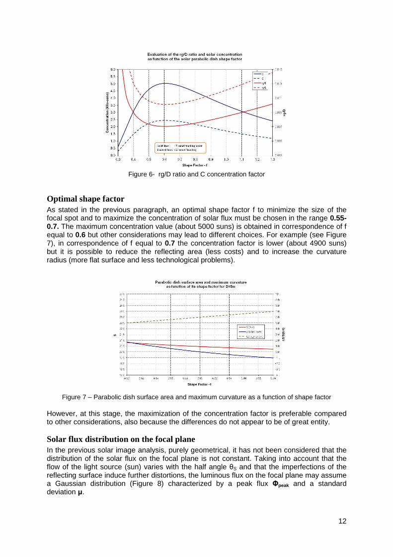
Figure 6- rg/D ratio and C concentration factor
Optimal shape factor As stated in the previous paragraph, an optimal shape factor f to minimize the size of the focal spot and to maximize the concentration of solar flux must be chosen in the range 0.55-0.7. The maximum concentration value (about 5000 suns) is obtained in correspondence of f equal to 0.6 but other considerations may lead to different choices. For example (see Figure 7), in correspondence of f equal to 0.7 the concentration factor is lower (about 4900 suns) but it is possible to reduce the reflecting area (less costs) and to increase the curvature radius (more flat surface and less technological problems).
Figure 7 – Parabolic dish surface area and maximum curvature as a function of shape factor
However, at this stage, the maximization of the concentration factor is preferable compared to other considerations, also because the differences do not appear to be of great entity.
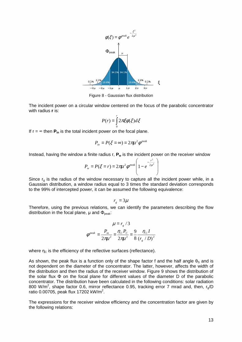
Solar flux distribution on the focal plane In the previous solar image analysis, purely geometrical, it has not been considered that the distribution of the solar flux on the focal plane is not constant. Taking into account that the flow of the light source (sun) varies with the half angle θS and that the imperfections of the reflecting surface induce further distortions, the luminous flux on the focal plane may assume a Gaussian distribution (Figure 8) characterized by a peak flux Φpeak and a standard deviation µ.
13
2
2
2)( µξ
φξφ−
= epeak
Figure 8 - Gaussian flux distribution
The incident power on a circular window centered on the focus of the parabolic concentrator with radius r is:
∫=r
drP0
)(2)( ξξπξφ
If r = ∞ then Pin is the total incident power on the focal plane.
peakin PP φπµξ 22)( =∞==
Instead, having the window a finite radius r, Pw is the incident power on the receiver window
−===
−2
2
22 12)( µφπµξr
peakw erPP
Since rg is the radius of the window necessary to capture all the incident power while, in a Gaussian distribution, a window radius equal to 3 times the standard deviation corresponds to the 99% of intercepted power, it can be assumed the following equivalence:
µ3=gr
Therefore, using the previous relations, we can identify the parameters describing the flow distribution in the focal plane, µ and Φpeak:
3/gr=µ
222 )/(8
9
22 Dr
IPP
g
CCCinpeak ηπµ
ηπµ
φ ===
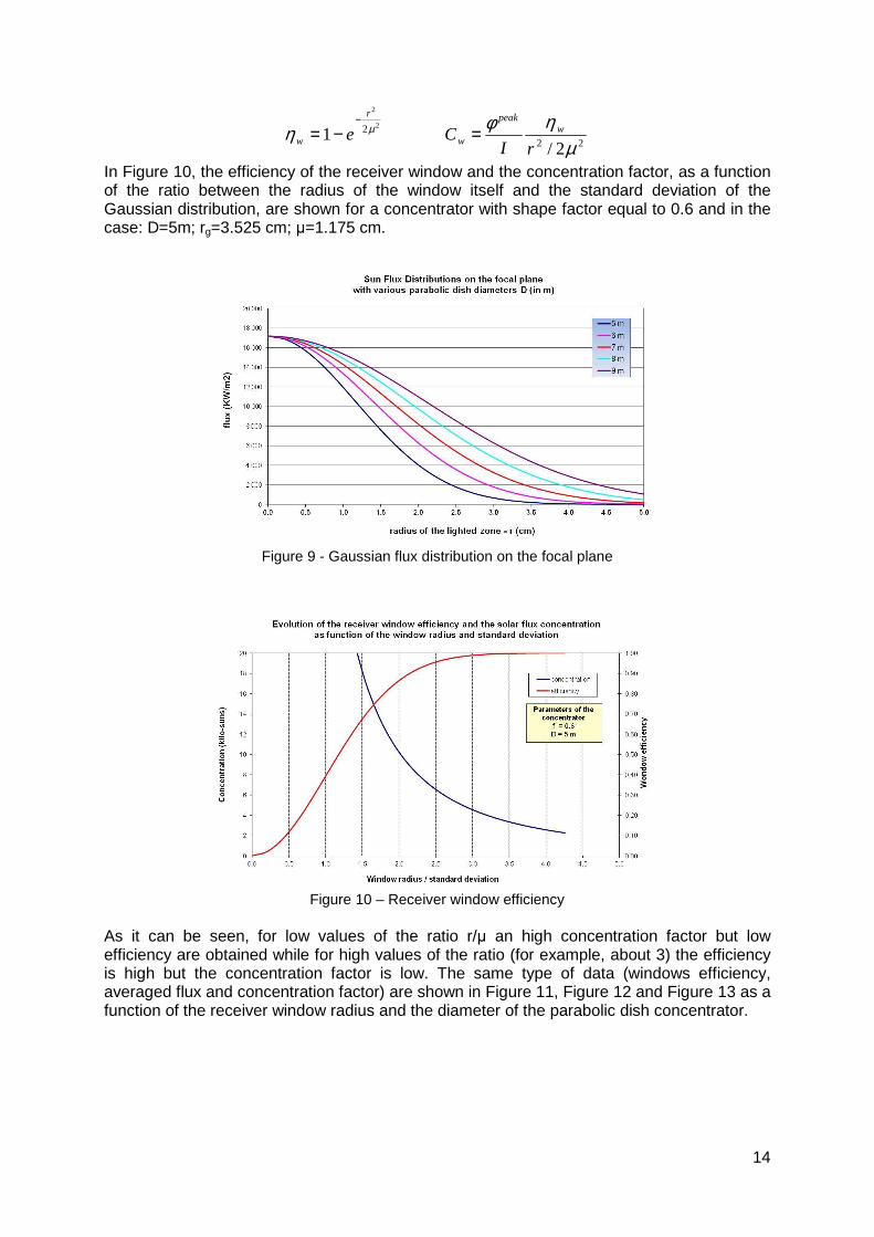
where ηC is the efficiency of the reflective surfaces (reflectance). As shown, the peak flux is a function only of the shape factor f and the half angle θS and is not dependent on the diameter of the concentrator. The latter, however, affects the width of the distribution and then the radius of the receiver window. Figure 9 shows the distribution of the solar flux Φ on the focal plane for different values of the diameter D of the parabolic concentrator. The distribution have been calculated in the following conditions: solar radiation 800 W/m2, shape factor 0.6, mirror reflectance 0.95, tracking error 7 mrad and, then, rg/D ratio 0.00705, peak flux 17202 kW/m2. The expressions for the receiver window efficiency and the concentration factor are given by the following relations:
Φpeak
ξ
14
2
2
21 µηr
w e−
−= 22 2/ µ
ηφrI
C wpeak
w =
In Figure 10, the efficiency of the receiver window and the concentration factor, as a function of the ratio between the radius of the window itself and the standard deviation of the Gaussian distribution, are shown for a concentrator with shape factor equal to 0.6 and in the case: D=5m; rg=3.525 cm; µ=1.175 cm.
Figure 9 - Gaussian flux distribution on the focal plane
Figure 10 – Receiver window efficiency
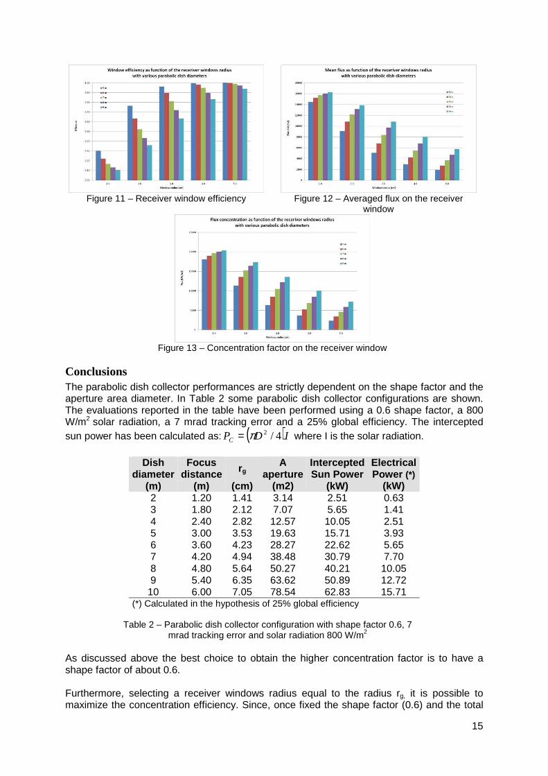
As it can be seen, for low values of the ratio r/µ an high concentration factor but low efficiency are obtained while for high values of the ratio (for example, about 3) the efficiency is high but the concentration factor is low. The same type of data (windows efficiency, averaged flux and concentration factor) are shown in Figure 11, Figure 12 and Figure 13 as a function of the receiver window radius and the diameter of the parabolic dish concentrator.
15
Figure 11 – Receiver window efficiency Figure 12 – Averaged flux on the receiver
window
Figure 13 – Concentration factor on the receiver window
Conclusions The parabolic dish collector performances are strictly dependent on the shape factor and the aperture area diameter. In Table 2 some parabolic dish collector configurations are shown. The evaluations reported in the table have been performed using a 0.6 shape factor, a 800 W/m2 solar radiation, a 7 mrad tracking error and a 25% global efficiency. The intercepted sun power has been calculated as: ( )IDPC 4/2π= where I is the solar radiation.
Dish
diameter Focus
distance rg A
aperture Intercepted Sun Power
Electrical Power (*)
(m) (m) (cm) (m2) (kW) (kW) 2 1.20 1.41 3.14 2.51 0.63 3 1.80 2.12 7.07 5.65 1.41 4 2.40 2.82 12.57 10.05 2.51 5 3.00 3.53 19.63 15.71 3.93 6 3.60 4.23 28.27 22.62 5.65 7 4.20 4.94 38.48 30.79 7.70 8 4.80 5.64 50.27 40.21 10.05 9 5.40 6.35 63.62 50.89 12.72
10 6.00 7.05 78.54 62.83 15.71 (*) Calculated in the hypothesis of 25% global efficiency
Table 2 – Parabolic dish collector configuration with shape factor 0.6, 7 mrad tracking error and solar radiation 800 W/m2
As discussed above the best choice to obtain the higher concentration factor is to have a shape factor of about 0.6. Furthermore, selecting a receiver windows radius equal to the radius rg, it is possible to maximize the concentration efficiency. Since, once fixed the shape factor (0.6) and the total
16
tracking error (7mrad), the minimum value for the ratio rg/D is equal to 0.00705, the selection of the radius rg is dependent on the diameter: as an example if the selected D is equal to 5 m, the diameter of the receiver window will be about 7 cm, while if D is equal to 8 m, the receiver window diameter will be about 20 cm. Actually, with the aim of optimizing the overall efficiency of the system, the choice of the receiver window diameter should be made taking into account the energy balance of the receiver and not only the optical aspects. This aspect will be analysed in the following chapter.
Efficiency evaluation
In the following analysis a cavity receiver with an aperture window radius r is considered. The absorption efficiency, defined as the ratio between the useful extracted power and the intercepted solar power is given by:
caWinCass ηηηηη ***=
where: • ηass : solar energy absorption efficiency • ηC : concentrator reflection efficiency • ηin : focal plane incident power collection efficiency • ηW : window transmission efficiency • ηca : conversion in useful power efficiency
Concentrator reflection efficiency The ability of the parabolic mirrors to reflect the solar intercepted power Pc to the focal plane (reflectance) is expressed as:
95.0==c
inC P
Pη
This efficiency is usually equal to about 95%.
Focal plane incident power collection efficiency This efficiency is the ratio of the effective power collected by the receiver window Pw and the total power distributed on the focal plane Pin. It is a function of the window aperture radius and is equal to:
−==
−2
2
21 µηr
in
win e
P
P
Window transmission efficiency The window transumission efficiency is the ratio between the power transmitted to the cavity Paw and that incident on the window Pw. Given the complexity of the phenomena of absorption/reflection occurring inside the cavity the transmission efficiency can be assumed equal to the apparent absorbance αw of the window.
ww
aww P
P αη ==
For a black body, the apparent absorbance is 1.
17
Conversion in useful power efficiency The conversion in useful power efficiency is the ratio between the useful power Pu absorbed by the cavity and the power transmitted to the cavity Paw. The useful power is thus a function of the power lost from the cavity. Ignoring losses by conduction and convection, the predominant losses, given the high temperature level, are those due to reirradiation from the cavity through the window aperture Prw.:
)( 24 rTP wrw πσε=
where σ is the Stefan-Boltzman constant and εw the emissivity of the cavity, that for a black body is 1. So, the cavity efficiency can be expressed in the following way:
aw
w
aw
rw
aw
rwaw
aw
uca P
rT
P
P
P
PP
P
P )(11
24 πσεη −=−=−
==
Absorption efficiency Taking into consideration the definitions adopted for the different efficiency terms, the complete expression for the absorption efficiency of the concentrator/receiver system is:
−
−=
−
aw
wW
r
Cass P
rTe
)(11
242 2
2
πσεαηη µ
This relation can also be written in the following form:
−
−=
− 242
21
2
2
µφσεαηη µ rT
epicco
in
w
r
WCass
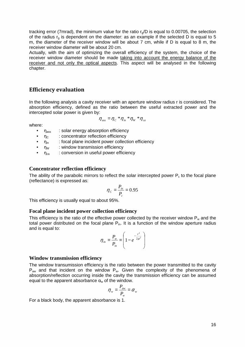
Once the characteristics of the concentrator are fixed, the absorption efficiency is only function of the radius r of the window aperture and the cavity average temperature T. In Figure 14, the trend of the absorption efficiency as a function of the ratio r/µ for different operating temperatures of the cavity, in the hypothesis that the receiver behaves as a black body, that the concentrator has a shape factor f equal to 0.6 and that the solar irradiation is equal to 800 W/m2, is shown.
Figure 14 – Absorption efficiency
18
It can be seen in all reported cases the presence of a maximum for the absorption efficiency. Increasing the cavity temperature, this maximum decreases and shifts to lower valuesof the r/µ ratio. At temperatures below 1000 °C an efficiency of over 90% is reached at values of r/µ equal to 3, then remaining almost constant.
Maximum cavity temperature The maximum temperature reached in the cavity is that for which the absorption efficiency is null (ηass = 0) or the power absorbed by the cavity equals the power lost by radiation (Paw = Prw):
)( 24 rTP wwW πσεα =
from which: 4/14/1
2max
ˆ
)(
=
=
w
w
w
ww IC
r
PT
σεα
πσεα
where: IIr
PC ww φ
π==
)(ˆ
2
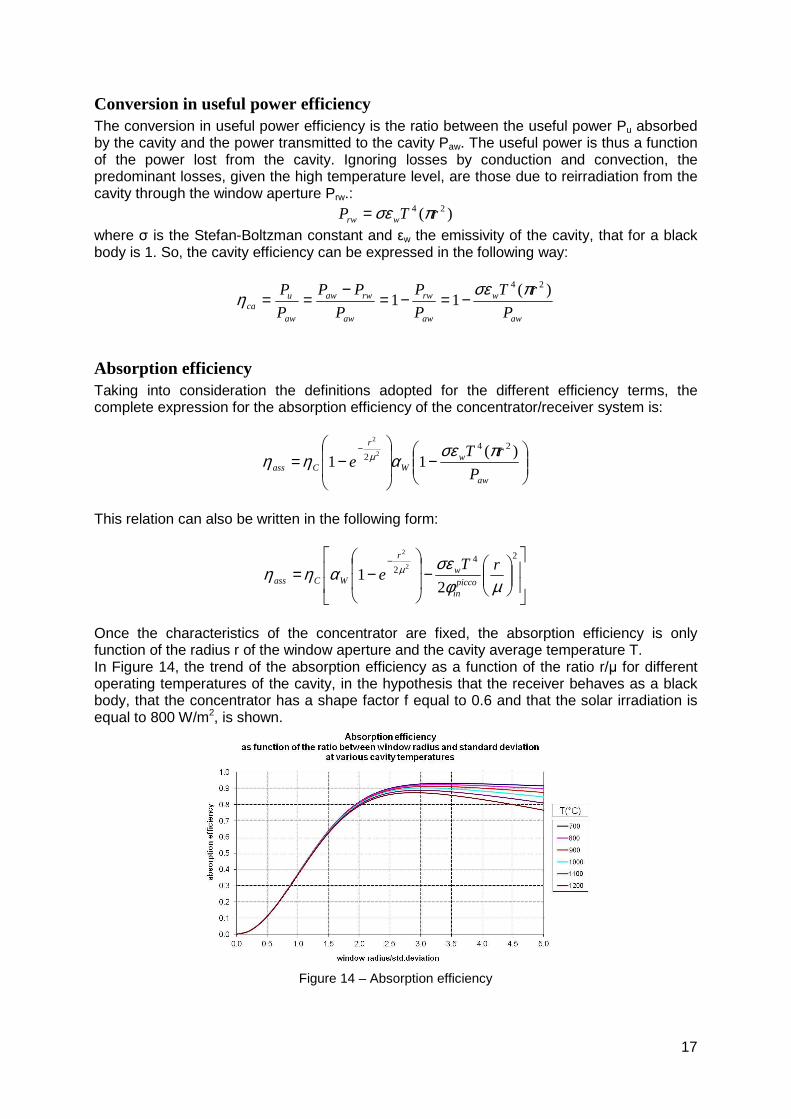
represents the concentration factor on the window of the cavity.
Figure 15 – Maximum cavity temperature and concentration
Total efficiency The useful power is used as heat in high temperature processes for guiding, for example, endothermic chemical reactions. The conversion of process heat into work or into Gibbs free energy of the reaction products is limited by the efficiency of Carnot. Then, for an ideal system, having indicated with TL the temperature of the cold sink, the efficiency of Carnot is:
T
TLCarnot −= 1η
Therefore, the total efficiency will be:
Carnotasstot ηηη ⋅=
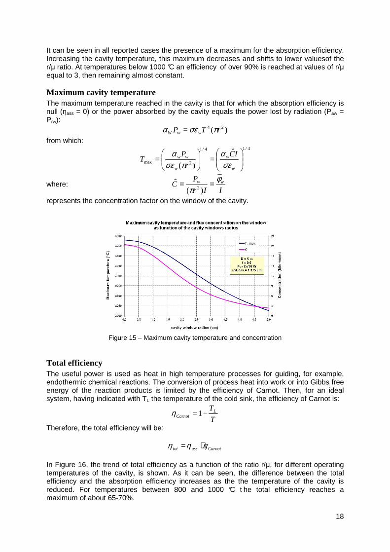
In Figure 16, the trend of total efficiency as a function of the ratio r/µ, for different operating temperatures of the cavity, is shown. As it can be seen, the difference between the total efficiency and the absorption efficiency increases as the the temperature of the cavity is reduced. For temperatures between 800 and 1000 °C t he total efficiency reaches a maximum of about 65-70%.
19
Figure 16 – Total efficiency
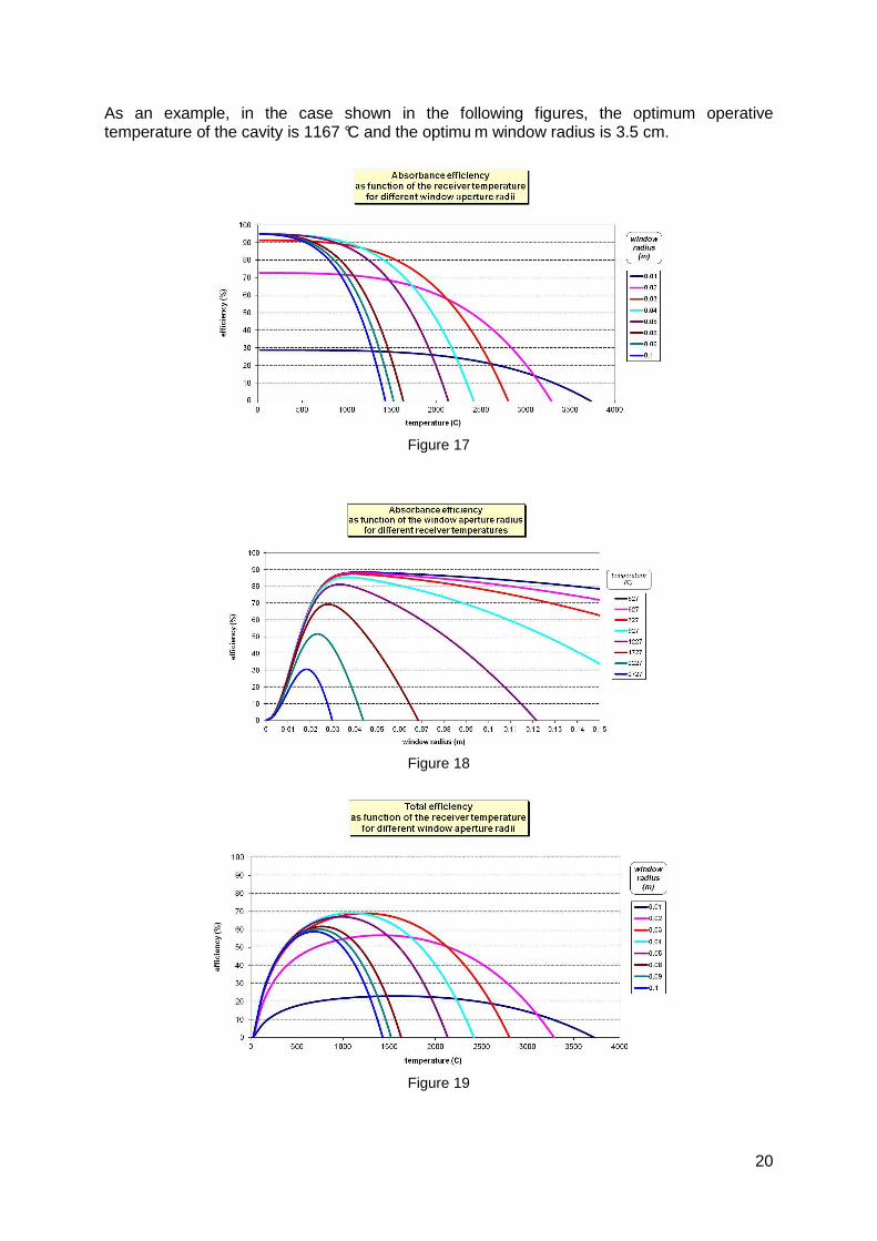
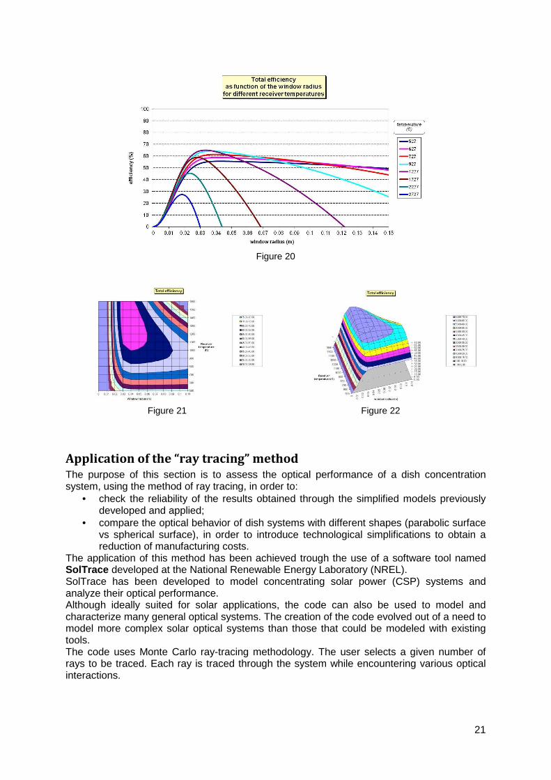
Therefore, it is evident, both from the relations previously reported and from the following figures (from Figure 17 to Figure 22), referring to the same conditions as in Figure 14, the total efficiency of the system is highly dependent on the temperature of the cavity and on the radius of the window aperture of the cavity itself. Then, an optimal operative zone exists, where the efficiency reaches its maximum values. The optimal values for r and T, corresponding to the maximum value of the efficiency, can be found imposing the following conditions:
=∂
∂
=∂
∂
0
0
T
rtot
tot
η
η
From the first condition it is possible to define the optimal value for the window aperture radius:
( )[ ] 5.02 )(ln2 optopt TXr µ−=
where : picco
inw
w TTX
φασε 4
)( =
while, from the second condition, a not explicit relation allows, using an iterative procedure, to find the optimal value for the temperature:
( ) 0))(1())(ln()(34 =−+− TXTTXTXTT LL A possible iterative schema is the following:
nifor
TTT
TTT
TXTX
TXTT
TT
iii
iii
ii
iLi
,......1
3.0
))(ln()())(1(
34
2/
)()1()(
)1()(0
)(
1()1(
)1()(
0
max)0(
=∆+=
−=∆
−−=
=
−
−
−−
−
20
As an example, in the case shown in the following figures, the optimum operative temperature of the cavity is 1167 °C and the optimu m window radius is 3.5 cm.
Figure 17
Figure 18
Figure 19
21
Figure 20
Figure 21 Figure 22
Application of the “ray tracing” method
The purpose of this section is to assess the optical performance of a dish concentration system, using the method of ray tracing, in order to:
• check the reliability of the results obtained through the simplified models previously developed and applied;
• compare the optical behavior of dish systems with different shapes (parabolic surface vs spherical surface), in order to introduce technological simplifications to obtain a reduction of manufacturing costs.
The application of this method has been achieved trough the use of a software tool named SolTrace developed at the National Renewable Energy Laboratory (NREL). SolTrace has been developed to model concentrating solar power (CSP) systems and analyze their optical performance. Although ideally suited for solar applications, the code can also be used to model and characterize many general optical systems. The creation of the code evolved out of a need to model more complex solar optical systems than those that could be modeled with existing tools. The code uses Monte Carlo ray-tracing methodology. The user selects a given number of rays to be traced. Each ray is traced through the system while encountering various optical interactions.
22
General settings The optical behavior of a dish concentrator, characterized by the following main parameters, has been simulated:
Parameter Value
Aperture diameter (m) 5
Aperture area (m2) 19.635
Focal plane quote (m) 3
Direct Normal Irradiance - DNI (W/m2) 1000
Intercepted solar power (W) 19635
Number of traced solar rays 1000000
Power for each solar ray 0.019635
Mirror reflectivity 0.95
Sun shape error (mrad) 2.73
Mirror slope error (mrad) 3.22
Mirror specularity (mrad) 0
Mirror optical error (mrad) 6.44
Total tracking error (mrad) 7
Table 3 – Main parameters used in the SolTrace simulations
As stated in the simplified models, the total tracking error is 7 mrad. To obtain this error the sun shape and optical errors (mirrors, slope and specularity) have been assigned to satisfy the following relationship:
22222 4 specslopesunoptsuntot σσσσσσ ++=+= (mrad)
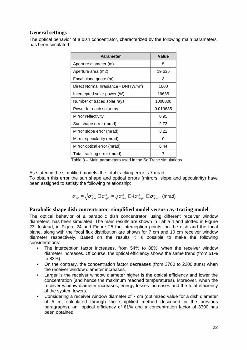
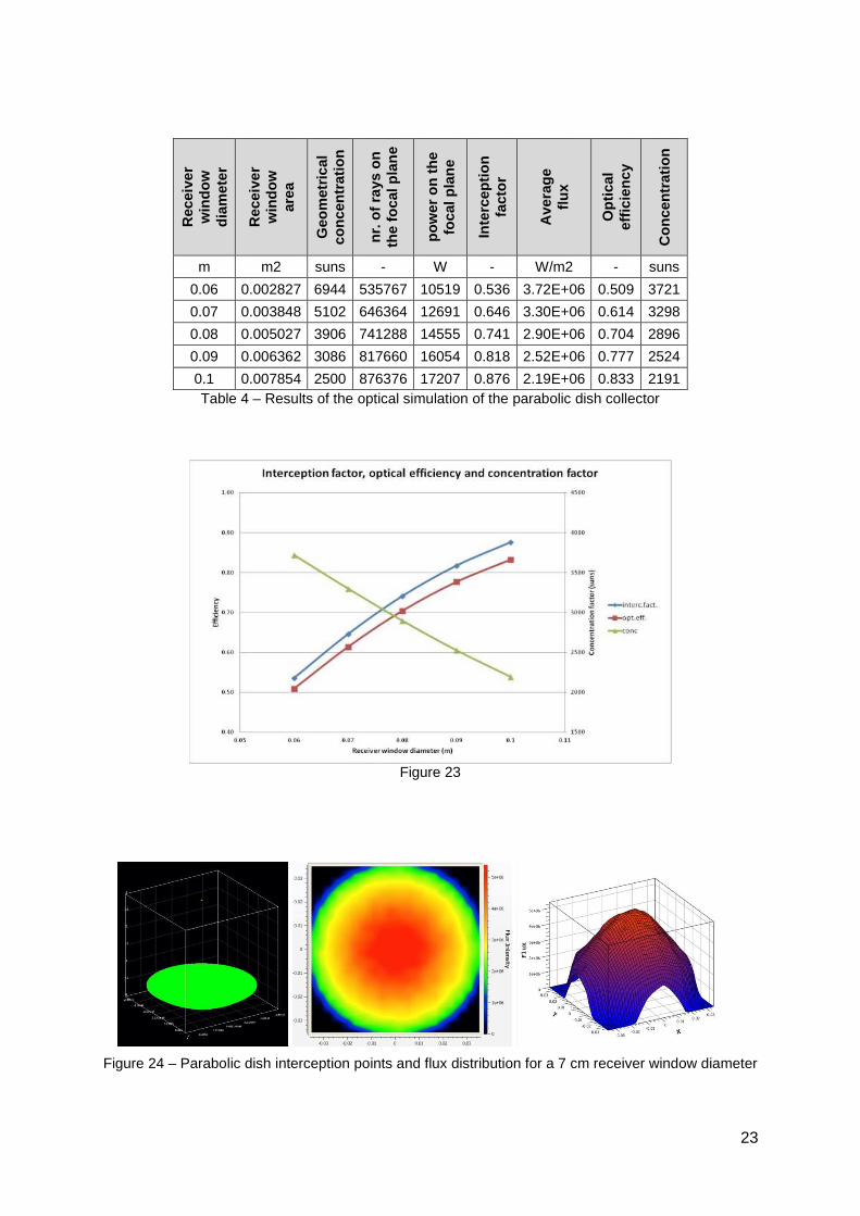
Parabolic shape dish concentrator: simplified model versus ray-tracing model The optical behavior of a parabolic dish concentrator, using different receiver window diameters, has been simulated. The main results are shown in Table 4 and plotted in Figure 23. Instead, in Figure 24 and Figure 25 the interception points, on the dish and the focal plane, along with the focal flux distribution are shown for 7 cm and 10 cm receiver window diameter respectively. Based on the results it is possible to make the following considerations:
• The interception factor increases, from 54% to 88%, when the receiver window diameter increases. Of course, the optical efficiency shows the same trend (from 51% to 83%).
• On the contrary, the concentration factor decreases (from 3700 to 2200 suns) when the receiver window diameter increases.
• Larger is the receiver window diameter higher is the optical efficiency and lower the concentration (and hence the maximum reached temperatures). Moreover, when the receiver window diameter increases, energy losses increases and the total efficiency of the system lowers.
• Considering a receiver window diameter of 7 cm (optimized value for a dish diameter of 5 m, calculated through the simplified method described in the previous paragraphs), an optical efficiency of 61% and a concentration factor of 3300 has been obtained.
23
Rec
eive
r w
indo
w
diam
eter
Rec
eive
r w
indo
w
area
Geo
met
rical
co
ncen
trat
ion
nr. o
f ray
s on
th
e fo
cal p
lane
pow
er o
n th
e fo
cal p
lane
Inte
rcep
tion
fact
or
Ave
rage
flu
x
Opt
ical
ef
ficie
ncy
Con
cent
ratio
n
m m2 suns - W - W/m2 - suns
0.06 0.002827 6944 535767 10519 0.536 3.72E+06 0.509 3721
0.07 0.003848 5102 646364 12691 0.646 3.30E+06 0.614 3298
0.08 0.005027 3906 741288 14555 0.741 2.90E+06 0.704 2896
0.09 0.006362 3086 817660 16054 0.818 2.52E+06 0.777 2524
0.1 0.007854 2500 876376 17207 0.876 2.19E+06 0.833 2191 Table 4 – Results of the optical simulation of the parabolic dish collector
Figure 23
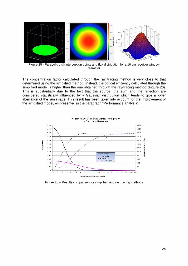
Figure 24 – Parabolic dish interception points and flux distribution for a 7 cm receiver window diameter
24
Figure 25 - Parabolic dish interception points and flux distribution for a 10 cm receiver window
diameter
The concentration factor calculated through the ray tracing method is very close to that determined using the simplified method. Instead, the optical efficiency calculated through the simplified model is higher than the one obtained through the ray-tracing method (Figure 26). This is substantially due to the fact that the source (the sun) and the reflection are considered statistically influenced by a Gaussian distribution which tends to give a lower aberration of the sun image. This result has been taken into account for the improvement of the simplified model, as presented in the paragraph “Performance analysis”.
Figure 26 – Results comparison for simplified and ray tracing methods
25
Spherical shape dish concentrator The ideal shape of a parabolic dish concentrator is surely a paraboloid of revolution. The surface so generated has the characteristic to have a variable curvature from the center of the disc to its periphery. This could represent a problem especially in the production of large reflective surfaces. The possibility to approximate such a parabolic surface with a spherical one, at constant curvature, would represent a simplification in terms of construction technology with a consequent lowering of the production costs. The main drawback, being no longer a figure with a punctual fire, might be to have an aberration of the sunlight beams with a significant loss of efficiency. Then, with the aim of evaluating the different performance of the parabolic and spherical concentrators, some optical simulations, described below, have been conducted. In this analysis, for the same aperture area, the paraboloid of revolution is replaced by a spherical surface having a radius two times the focal distance (r = 2f).
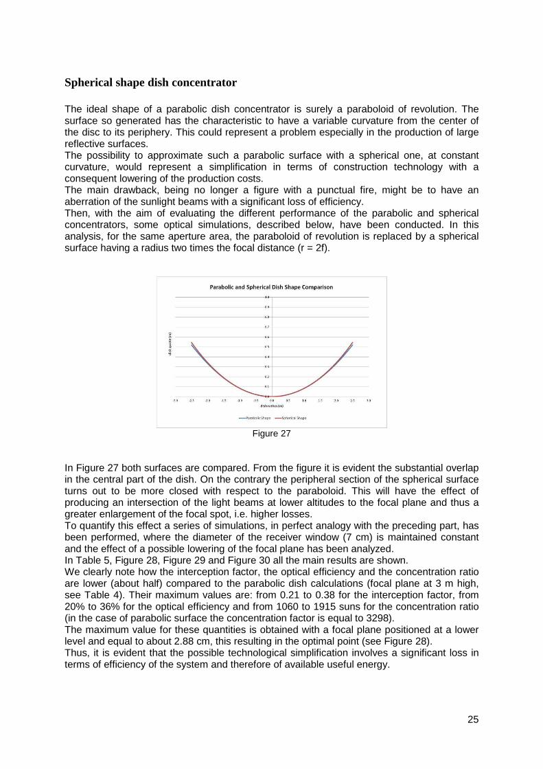
Figure 27
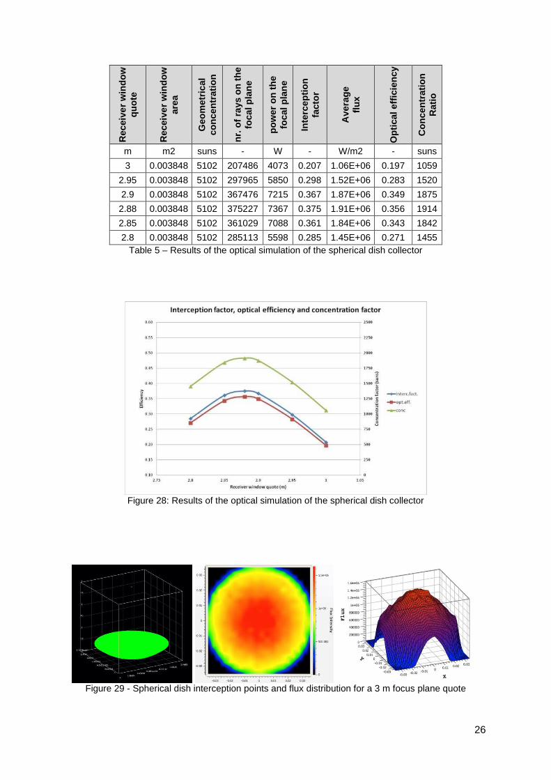
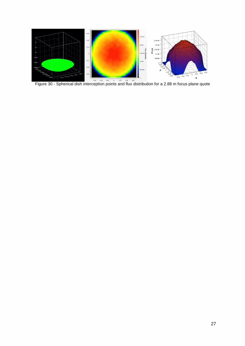
In Figure 27 both surfaces are compared. From the figure it is evident the substantial overlap in the central part of the dish. On the contrary the peripheral section of the spherical surface turns out to be more closed with respect to the paraboloid. This will have the effect of producing an intersection of the light beams at lower altitudes to the focal plane and thus a greater enlargement of the focal spot, i.e. higher losses. To quantify this effect a series of simulations, in perfect analogy with the preceding part, has been performed, where the diameter of the receiver window (7 cm) is maintained constant and the effect of a possible lowering of the focal plane has been analyzed. In Table 5, Figure 28, Figure 29 and Figure 30 all the main results are shown. We clearly note how the interception factor, the optical efficiency and the concentration ratio are lower (about half) compared to the parabolic dish calculations (focal plane at 3 m high, see Table 4). Their maximum values are: from 0.21 to 0.38 for the interception factor, from 20% to 36% for the optical efficiency and from 1060 to 1915 suns for the concentration ratio (in the case of parabolic surface the concentration factor is equal to 3298). The maximum value for these quantities is obtained with a focal plane positioned at a lower level and equal to about 2.88 cm, this resulting in the optimal point (see Figure 28). Thus, it is evident that the possible technological simplification involves a significant loss in terms of efficiency of the system and therefore of available useful energy.
26
Rec
eive
r w
indo
w
quot
e
Rec
eive
r w
indo
w
area
Geo
met
rical
co
ncen
trat
ion
nr. o
f ray
s on
the
foca
l pla
ne
pow
er o
n th
e fo
cal p
lane
Inte
rcep
tion
fact
or
Ave
rage
flu
x
Opt
ical
effi
cien
cy
Con
cent
ratio
n R
atio
m m2 suns - W - W/m2 - suns
3 0.003848 5102 207486 4073 0.207 1.06E+06 0.197 1059
2.95 0.003848 5102 297965 5850 0.298 1.52E+06 0.283 1520
2.9 0.003848 5102 367476 7215 0.367 1.87E+06 0.349 1875
2.88 0.003848 5102 375227 7367 0.375 1.91E+06 0.356 1914
2.85 0.003848 5102 361029 7088 0.361 1.84E+06 0.343 1842
2.8 0.003848 5102 285113 5598 0.285 1.45E+06 0.271 1455 Table 5 – Results of the optical simulation of the spherical dish collector
Figure 28: Results of the optical simulation of the spherical dish collector
Figure 29 - Spherical dish interception points and flux distribution for a 3 m focus plane quote
27
Figure 30 - Spherical dish interception points and flux distribution for a 2.88 m focus plane quote
28
Conclusions
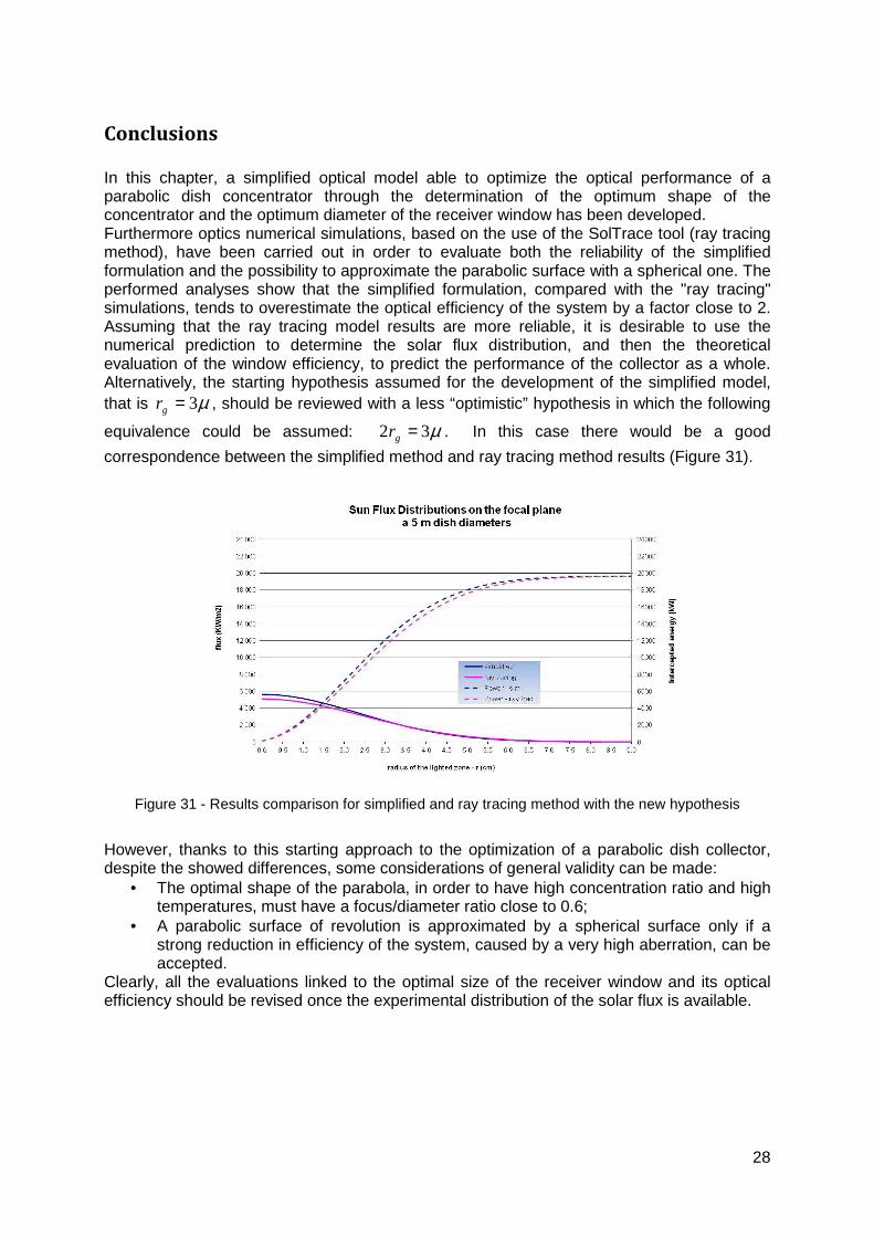
In this chapter, a simplified optical model able to optimize the optical performance of a parabolic dish concentrator through the determination of the optimum shape of the concentrator and the optimum diameter of the receiver window has been developed. Furthermore optics numerical simulations, based on the use of the SolTrace tool (ray tracing method), have been carried out in order to evaluate both the reliability of the simplified formulation and the possibility to approximate the parabolic surface with a spherical one. The performed analyses show that the simplified formulation, compared with the "ray tracing" simulations, tends to overestimate the optical efficiency of the system by a factor close to 2. Assuming that the ray tracing model results are more reliable, it is desirable to use the numerical prediction to determine the solar flux distribution, and then the theoretical evaluation of the window efficiency, to predict the performance of the collector as a whole. Alternatively, the starting hypothesis assumed for the development of the simplified model, that is µ3=gr , should be reviewed with a less “optimistic” hypothesis in which the following
equivalence could be assumed: µ32 =gr . In this case there would be a good
correspondence between the simplified method and ray tracing method results (Figure 31).
Figure 31 - Results comparison for simplified and ray tracing method with the new hypothesis
However, thanks to this starting approach to the optimization of a parabolic dish collector, despite the showed differences, some considerations of general validity can be made:
• The optimal shape of the parabola, in order to have high concentration ratio and high temperatures, must have a focus/diameter ratio close to 0.6;
• A parabolic surface of revolution is approximated by a spherical surface only if a strong reduction in efficiency of the system, caused by a very high aberration, can be accepted.
Clearly, all the evaluations linked to the optimal size of the receiver window and its optical efficiency should be revised once the experimental distribution of the solar flux is available.
29
Performance analysis
In the present paragraph a performance analysis of the solar dish collector proposed by Innova will be reported. As a starting hypothesis it has been assumed to use a 7kWe MGT with the following base conditions: maximum solar radiation (I) of about 800 W/m2, maximum global efficiency (ηtot) of about 20%, and utilization factor of the total area (fused) of 90%. In this case, we should get:
• A useful receiving surface: Snet = Pe/ (ηtot I) = 43.75 m2 ; • A total receiving surface: Stot = Snet / fused = 48.6 m2 ; • An aperture diameter of the parabolic dish: D = (4*Stot / π)^0.5 = 7.9 m
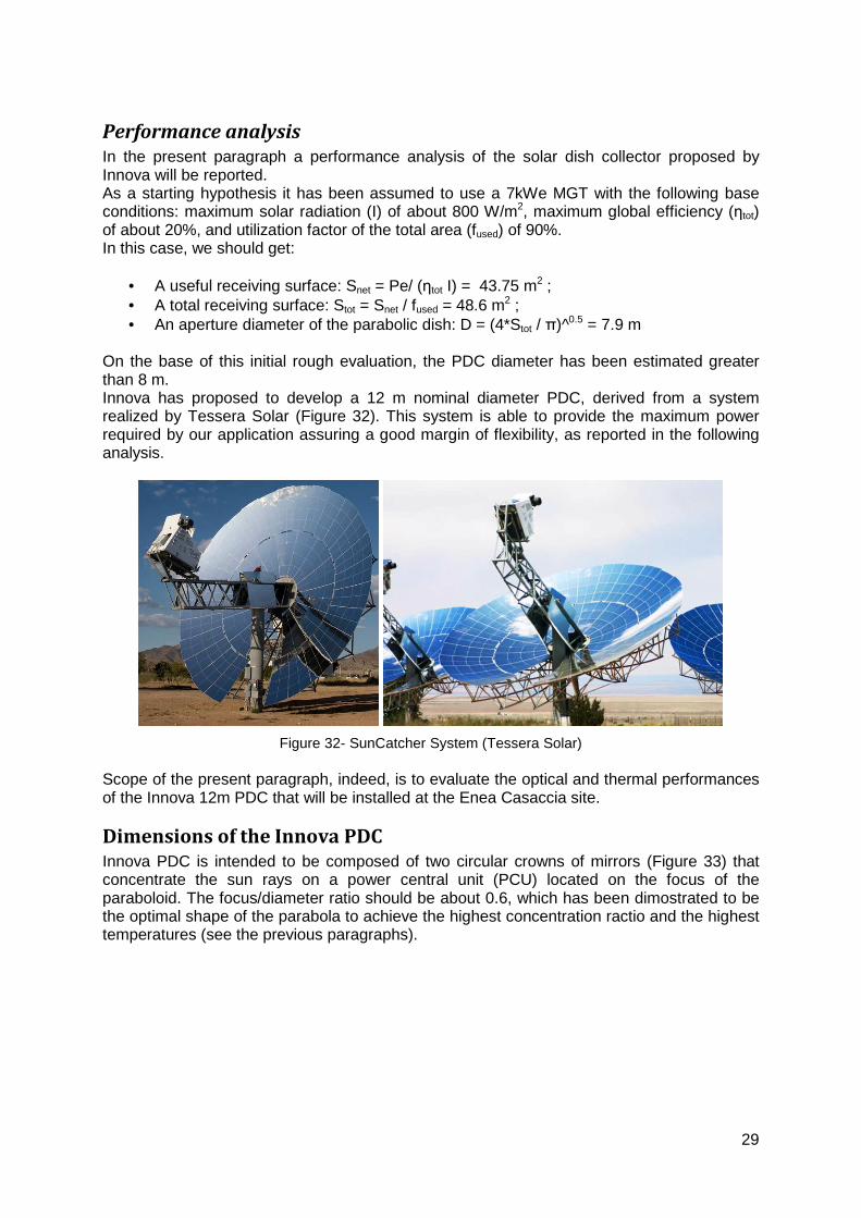
On the base of this initial rough evaluation, the PDC diameter has been estimated greater than 8 m. Innova has proposed to develop a 12 m nominal diameter PDC, derived from a system realized by Tessera Solar (Figure 32). This system is able to provide the maximum power required by our application assuring a good margin of flexibility, as reported in the following analysis.
Figure 32- SunCatcher System (Tessera Solar)
Scope of the present paragraph, indeed, is to evaluate the optical and thermal performances of the Innova 12m PDC that will be installed at the Enea Casaccia site.
Dimensions of the Innova PDC
Innova PDC is intended to be composed of two circular crowns of mirrors (Figure 33) that concentrate the sun rays on a power central unit (PCU) located on the focus of the paraboloid. The focus/diameter ratio should be about 0.6, which has been dimostrated to be the optimal shape of the parabola to achieve the highest concentration ractio and the highest temperatures (see the previous paragraphs).
30
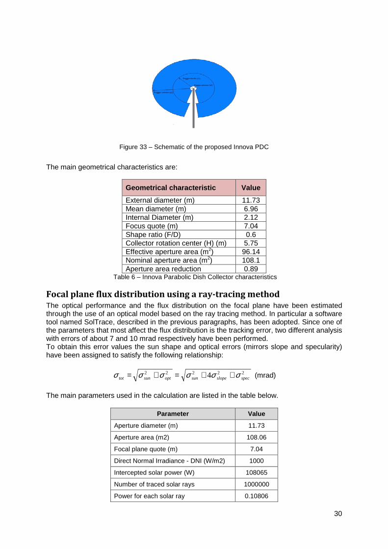
Figure 33 – Schematic of the proposed Innova PDC
The main geometrical characteristics are:
Geometrical characteristic Value
External diameter (m) 11.73 Mean diameter (m) 6.96 Internal Diameter (m) 2.12 Focus quote (m) 7.04 Shape ratio (F/D) 0.6 Collector rotation center (H) (m) 5.75 Effective aperture area (m2) 96.14 Nominal aperture area (m2) 108.1 Aperture area reduction 0.89
Table 6 – Innova Parabolic Dish Collector characteristics
Focal plane flux distribution using a ray-tracing method
The optical performance and the flux distribution on the focal plane have been estimated through the use of an optical model based on the ray tracing method. In particular a software tool named SolTrace, described in the previous paragraphs, has been adopted. Since one of the parameters that most affect the flux distribution is the tracking error, two different analysis with errors of about 7 and 10 mrad respectively have been performed. To obtain this error values the sun shape and optical errors (mirrors slope and specularity) have been assigned to satisfy the following relationship:
22222 4 specslopesunoptsuntot σσσσσσ ++=+= (mrad)
The main parameters used in the calculation are listed in the table below.
Parameter Value
Aperture diameter (m) 11.73
Aperture area (m2) 108.06
Focal plane quote (m) 7.04
Direct Normal Irradiance - DNI (W/m2) 1000
Intercepted solar power (W) 108065
Number of traced solar rays 1000000
Power for each solar ray 0.10806
31
Mirror reflectivity 0.95
Sun shape error (mrad) 2.73
Mirror slope error (mrad) 3.4 (4.6)
Mirror specularity (mrad) 1.2 (3.3)
Mirror optical error (mrad) 6.9 (9.8)
Total tracking error (mrad) 7.43 (10.14)
Table 7 – Main parameters used in the SolTrace simulations
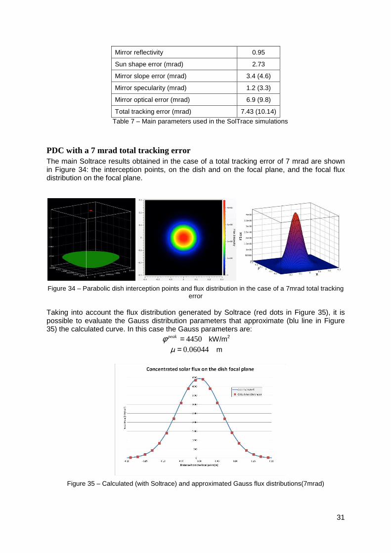
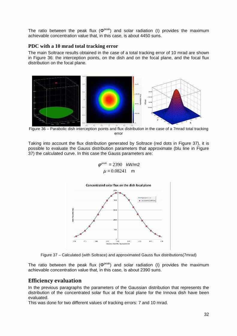
PDC with a 7 mrad total tracking error The main Soltrace results obtained in the case of a total tracking error of 7 mrad are shown in Figure 34: the interception points, on the dish and on the focal plane, and the focal flux distribution on the focal plane.
Figure 34 – Parabolic dish interception points and flux distribution in the case of a 7mrad total tracking
error Taking into account the flux distribution generated by Soltrace (red dots in Figure 35), it is possible to evaluate the Gauss distribution parameters that approximate (blu line in Figure 35) the calculated curve. In this case the Gauss parameters are:
4450=peakφ kW/m2
06044.0=µ m
Figure 35 – Calculated (with Soltrace) and approximated Gauss flux distributions(7mrad)
32
The ratio between the peak flux (Φpeak) and solar radiation (I) provides the maximum achievable concentration value that, in this case, is about 4450 suns.
PDC with a 10 mrad total tracking error The main Soltrace results obtained in the case of a total tracking error of 10 mrad are shown in Figure 36: the interception points, on the dish and on the focal plane, and the focal flux distribution on the focal plane.
Figure 36 – Parabolic dish interception points and flux distribution in the case of a 7mrad total tracking
error Taking into account the flux distribution generated by Soltrace (red dots in Figure 37), it is possible to evaluate the Gauss distribution parameters that approximate (blu line in Figure 37) the calculated curve. In this case the Gauss parameters are:
2390=peakφ kW/m2
08241.0=µ m
Figure 37 – Calculated (with Soltrace) and approximated Gauss flux distributions(7mrad)
The ratio between the peak flux (Φpeak) and solar radiation (I) provides the maximum achievable concentration value that, in this case, is about 2390 suns.
Efficiency evaluation
In the previous paragraphs the parameters of the Gaussian distribution that represents the distribution of the concentrated solar flux at the focal plane for the Innova dish have been evaluated. This was done for two different values of tracking errors: 7 and 10 mrad.
33
In the following table the results obtained are listed:
Total tracking error (mrad) 7 10
Peak flux (kW/m2) 4450 2390
Standard deviation µ (m) 0.06044 0.08241
Table 8 – Gauss distribution parameters for Innova 12m PDC
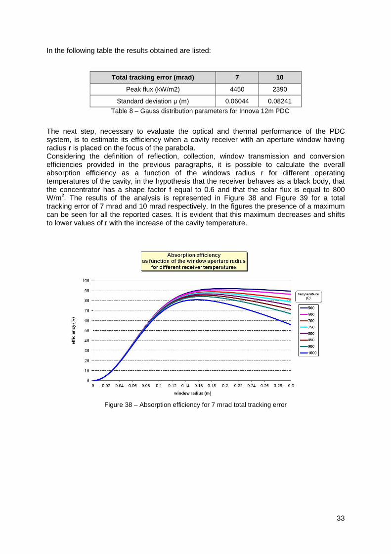
The next step, necessary to evaluate the optical and thermal performance of the PDC system, is to estimate its efficiency when a cavity receiver with an aperture window having radius r is placed on the focus of the parabola. Considering the definition of reflection, collection, window transmission and conversion efficiencies provided in the previous paragraphs, it is possible to calculate the overall absorption efficiency as a function of the windows radius r for different operating temperatures of the cavity, in the hypothesis that the receiver behaves as a black body, that the concentrator has a shape factor f equal to 0.6 and that the solar flux is equal to 800 W/m2. The results of the analysis is represented in Figure 38 and Figure 39 for a total tracking error of 7 mrad and 10 mrad respectively. In the figures the presence of a maximum can be seen for all the reported cases. It is evident that this maximum decreases and shifts to lower values of r with the increase of the cavity temperature.
Figure 38 – Absorption efficiency for 7 mrad total tracking error
34
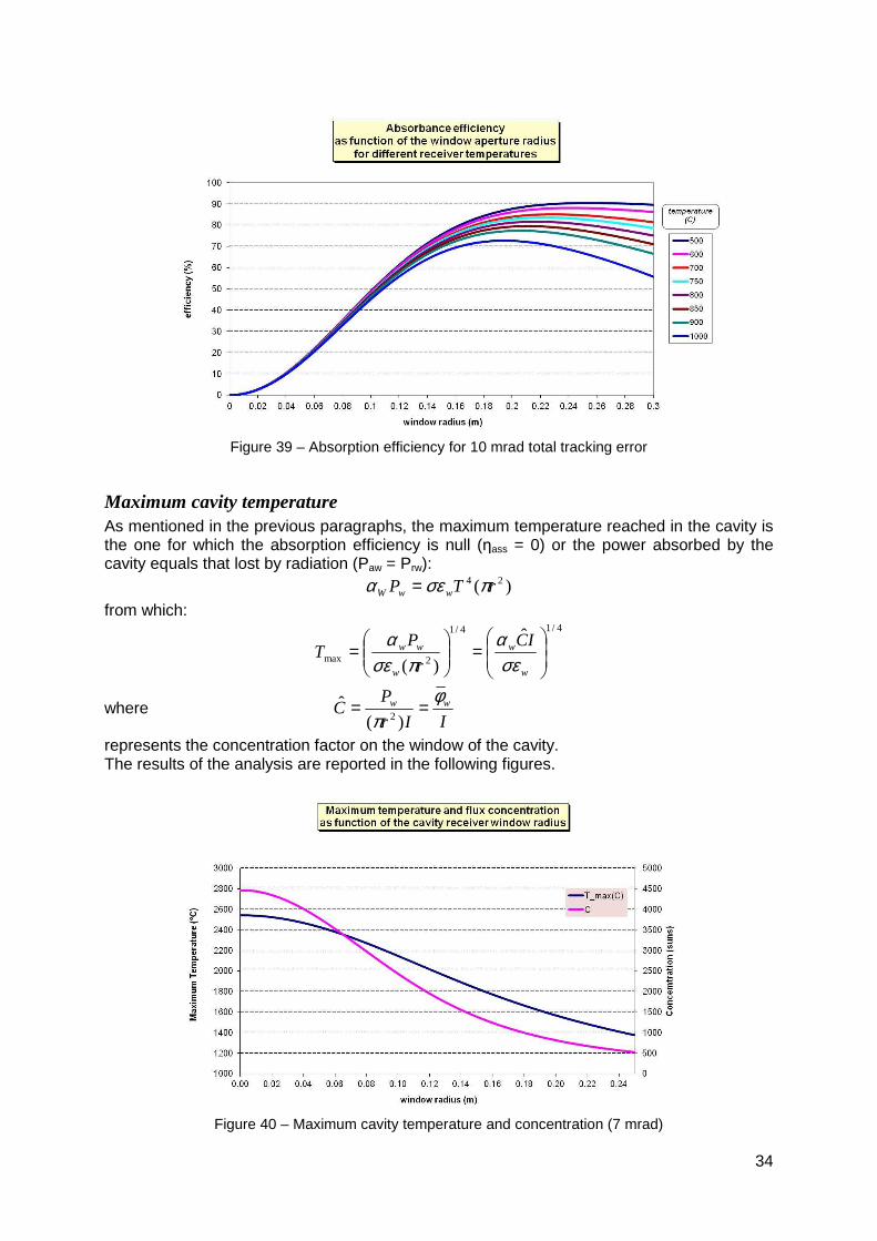
Figure 39 – Absorption efficiency for 10 mrad total tracking error
Maximum cavity temperature As mentioned in the previous paragraphs, the maximum temperature reached in the cavity is the one for which the absorption efficiency is null (ηass = 0) or the power absorbed by the cavity equals that lost by radiation (Paw = Prw):
)( 24 rTP wwW πσεα =
from which: 4/14/1
2max
ˆ
)(
=
=
w
w
w
ww IC
r
PT
σεα
πσεα
where IIr
PC ww φ
π==
)(ˆ
2
represents the concentration factor on the window of the cavity. The results of the analysis are reported in the following figures.
Figure 40 – Maximum cavity temperature and concentration (7 mrad)
35
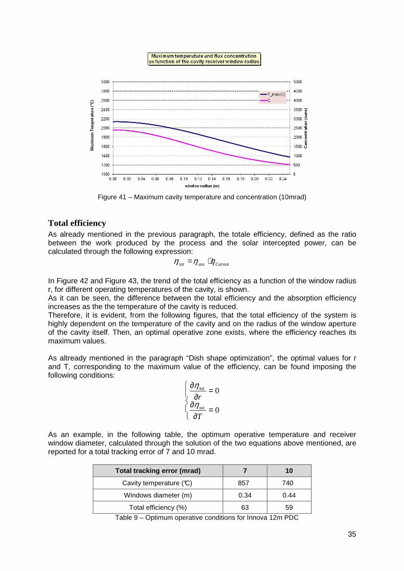
Figure 41 – Maximum cavity temperature and concentration (10mrad)
Total efficiency As already mentioned in the previous paragraph, the totale efficiency, defined as the ratio between the work produced by the process and the solar intercepted power, can be calculated through the following expression:
Carnotasstot ηηη ⋅=
In Figure 42 and Figure 43, the trend of the total efficiency as a function of the window radius r, for different operating temperatures of the cavity, is shown. As it can be seen, the difference between the total efficiency and the absorption efficiency increases as the the temperature of the cavity is reduced. Therefore, it is evident, from the following figures, that the total efficiency of the system is highly dependent on the temperature of the cavity and on the radius of the window aperture of the cavity itself. Then, an optimal operative zone exists, where the efficiency reaches its maximum values. As altready mentioned in the paragraph “Dish shape optimization”, the optimal values for r and T, corresponding to the maximum value of the efficiency, can be found imposing the following conditions:
=∂
∂
=∂
∂
0
0
T
rtot
tot
η
η
As an example, in the following table, the optimum operative temperature and receiver window diameter, calculated through the solution of the two equations above mentioned, are reported for a total tracking error of 7 and 10 mrad.
Total tracking error (mrad) 7 10
Cavity temperature (°C) 857 740
Windows diameter (m) 0.34 0.44
Total efficiency (%) 63 59
Table 9 – Optimum operative conditions for Innova 12m PDC
36
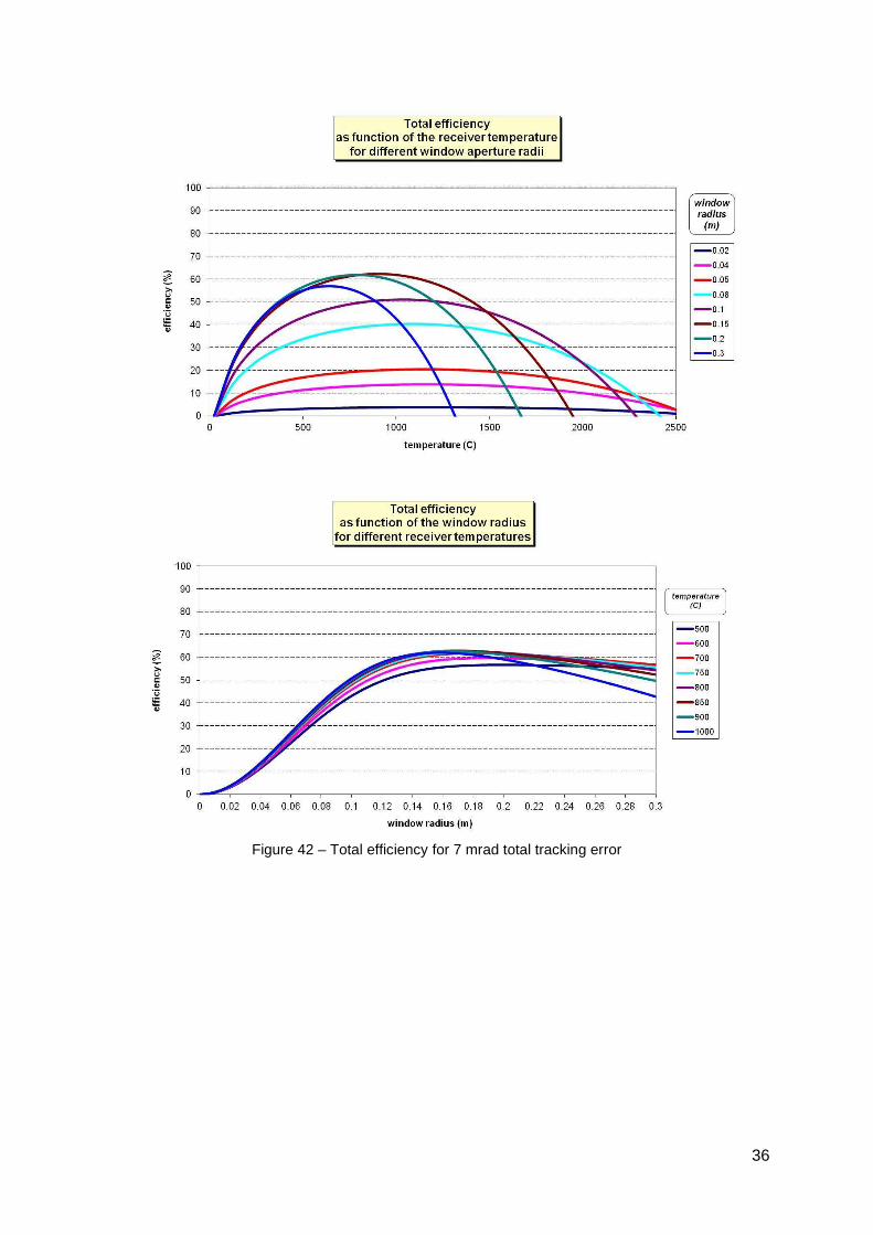
Figure 42 – Total efficiency for 7 mrad total tracking error
37
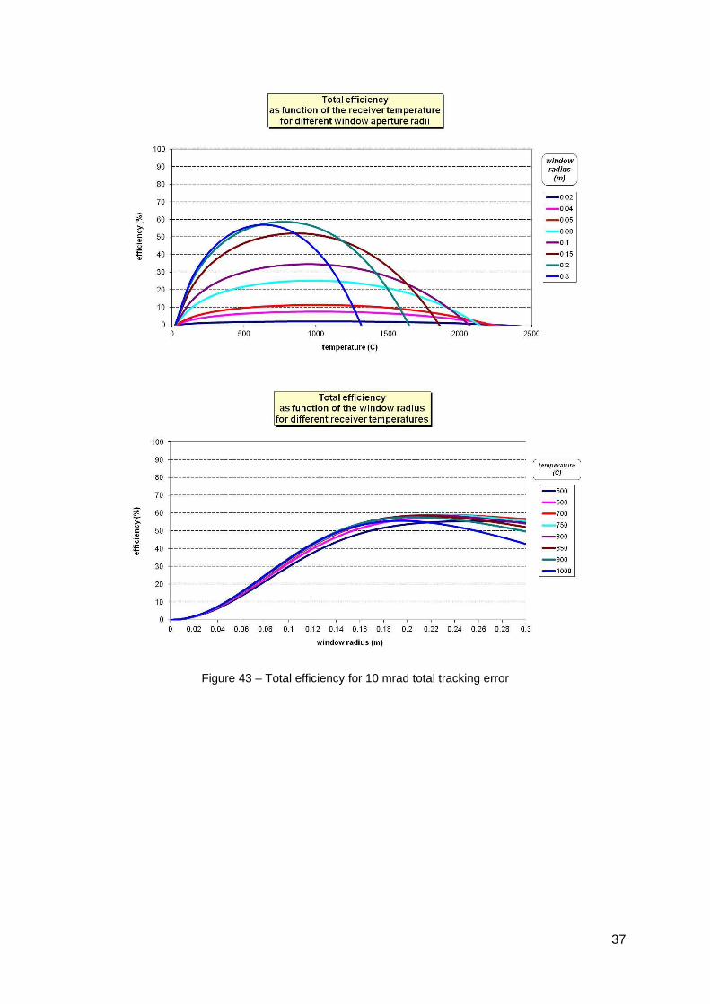
Figure 43 – Total efficiency for 10 mrad total tracking error
38
Conclusions
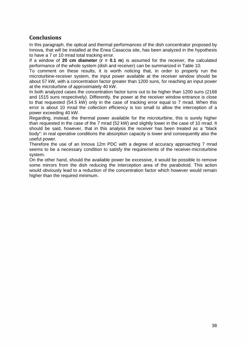
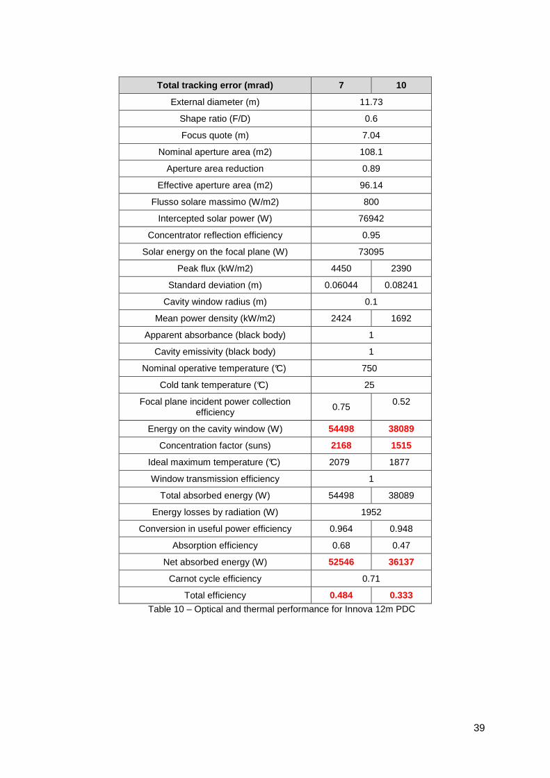
In this paragraph, the optical and thermal performances of the dish concentrator proposed by Innova, that will be installed at the Enea Casaccia site, has been analyzed in the hypothesis to have a 7 or 10 mrad total tracking error. If a window of 20 cm diameter (r = 0.1 m ) is assumed for the receiver, the calculated performance of the whole system (dish and receiver) can be summarized in Table 10. To comment on these results, it is worth noticing that, in order to properly run the microturbine-receiver system, the input power available at the receiver window should be about 57 kW, with a concentration factor greater than 1200 suns, for reaching an input power at the microturbine of approximately 40 kW. In both analyzed cases the concentration factor turns out to be higher than 1200 suns (2168 and 1515 suns respectively). Differently, the power at the receiver window entrance is close to that requested (54.5 kW) only in the case of tracking error equal to 7 mrad. When this error is about 10 mrad the collection efficiency is too small to allow the interception of a power exceeding 40 kW. Regarding, instead, the thermal power available for the microturbine, this is surely higher than requested in the case of the 7 mrad (52 kW) and slightly lower in the case of 10 mrad. It should be said, however, that in this analysis the receiver has been treated as a “black body”: in real operative conditions the absorption capacity is lower and consequently also the useful power. Therefore the use of an Innova 12m PDC with a degree of accuracy approaching 7 mrad seems to be a necessary condition to satisfy the requirements of the receiver-microturbine system. On the other hand, should the available power be excessive, it would be possible to remove some mirrors from the dish reducing the interception area of the paraboloid. This action would obviously lead to a reduction of the concentration factor which however would remain higher than the required minimum.
39
Total tracking error (mrad) 7 10
External diameter (m) 11.73
Shape ratio (F/D) 0.6
Focus quote (m) 7.04
Nominal aperture area (m2) 108.1
Aperture area reduction 0.89
Effective aperture area (m2) 96.14
Flusso solare massimo (W/m2) 800
Intercepted solar power (W) 76942
Concentrator reflection efficiency 0.95
Solar energy on the focal plane (W) 73095
Peak flux (kW/m2) 4450 2390
Standard deviation (m) 0.06044 0.08241
Cavity window radius (m) 0.1
Mean power density (kW/m2) 2424 1692
Apparent absorbance (black body) 1
Cavity emissivity (black body) 1
Nominal operative temperature (°C) 750
Cold tank temperature (°C) 25
Focal plane incident power collection efficiency
0.75 0.52
Energy on the cavity window (W) 54498 38089
Concentration factor (suns) 2168 1515
Ideal maximum temperature (°C) 2079 1877
Window transmission efficiency 1
Total absorbed energy (W) 54498 38089
Energy losses by radiation (W) 1952
Conversion in useful power efficiency 0.964 0.948
Absorption efficiency 0.68 0.47
Net absorbed energy (W) 52546 36137
Carnot cycle efficiency 0.71
Total efficiency 0.484 0.333
Table 10 – Optical and thermal performance for Innova 12m PDC
40
SIMUL-DISH: a portable ray tracing software for analytical dish
simulation (Marco Montecchi (ENEA)) In the previous chapters, optics and thermal-efficiency of dishes are discussed on the basis of some general assumptions. Particularly,the size of the solar spot concentrated at the focal plane is calculated by assuming that the statistical distribution of each important parameter is Gaussian. In particular two of them are very important: the divergence of solar radiation and the deviation of mirror shape from the ideal paraboloid. Indeed the Gaussian approach makes simpler the treatment by virtue of the property that linear combinations of normal (Gaussian) distributed variables is itself normal distributed. On the other hand, in clear sky conditions, the angular distribution of solar radiation is much more close to rectangular than Gaussian function. Moreover, since the surface of the facets composing the reflector is continuous, the shape deviation in two points of the same facet is highly correlated. Therefore the deviation behaves as a continuous curve with features that are quite systematic for a given production batch of facets. Finally, for practical convenience, very often the mirrored surface of dishes is shaped as an annulus with a missing slice. With the purposes of evaluating dish optical features in a more rigorous manner, the dedicated software SIMUL-DISH was developed. In the following its main features and some preliminary results are reported.
Software description
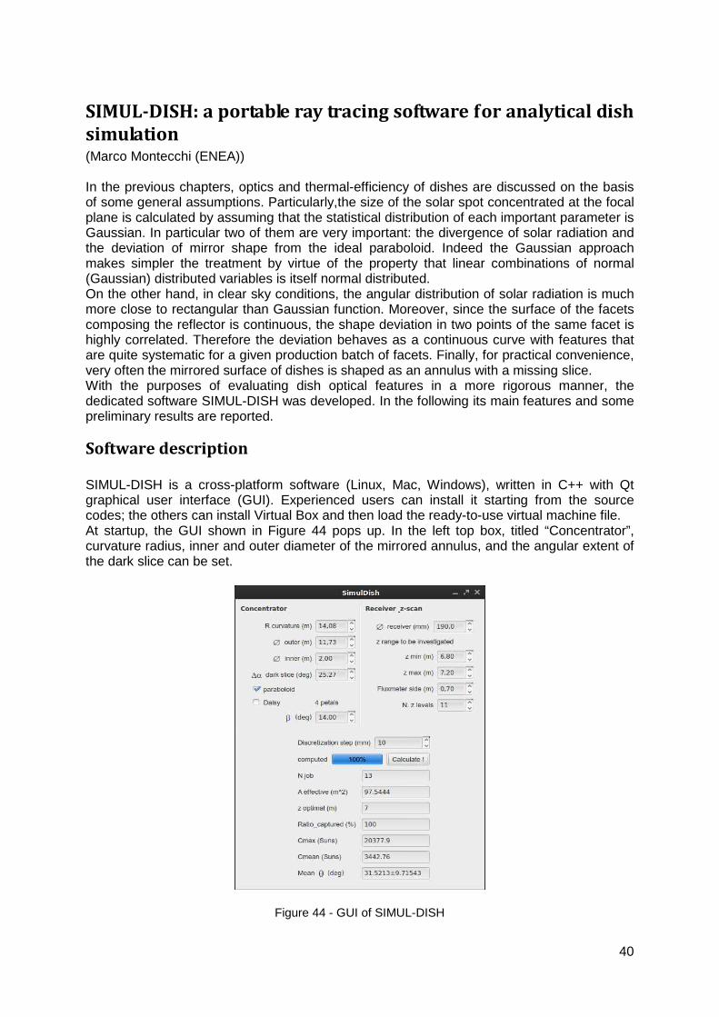
SIMUL-DISH is a cross-platform software (Linux, Mac, Windows), written in C++ with Qt graphical user interface (GUI). Experienced users can install it starting from the source codes; the others can install Virtual Box and then load the ready-to-use virtual machine file. At startup, the GUI shown in Figure 44 pops up. In the left top box, titled “Concentrator”, curvature radius, inner and outer diameter of the mirrored annulus, and the angular extent of the dark slice can be set.
Figure 44 - GUI of SIMUL-DISH
41
The surface is assumed parabolic , with f focal distance, if “paraboloid” is
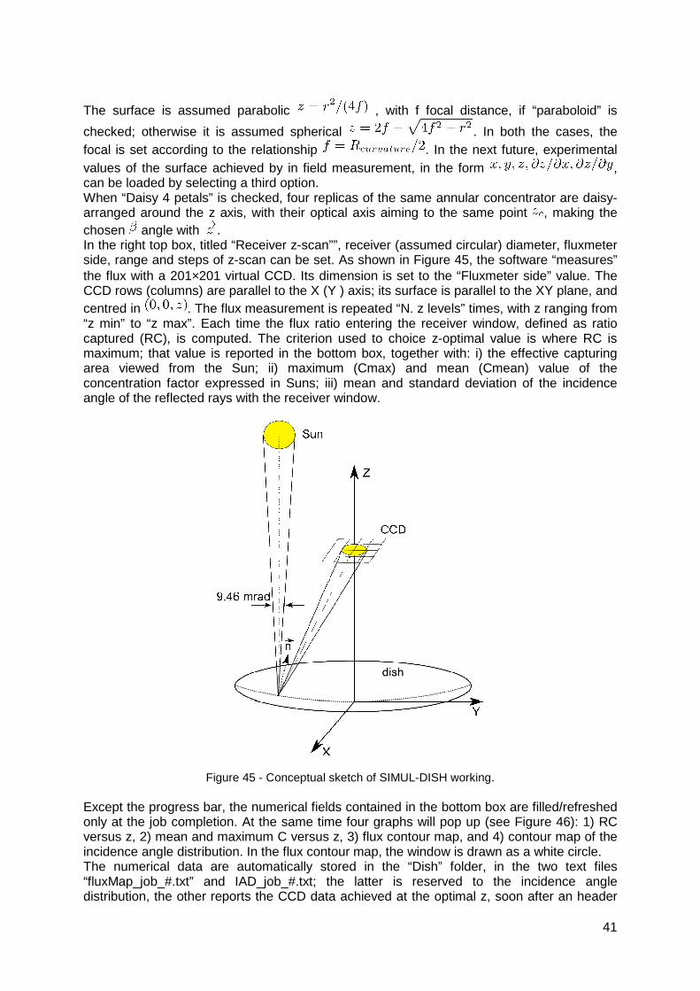
checked; otherwise it is assumed spherical . In both the cases, the focal is set according to the relationship . In the next future, experimental values of the surface achieved by in field measurement, in the form , can be loaded by selecting a third option. When “Daisy 4 petals” is checked, four replicas of the same annular concentrator are daisy-arranged around the z axis, with their optical axis aiming to the same point , making the chosen angle with . In the right top box, titled “Receiver z-scan””, receiver (assumed circular) diameter, fluxmeter side, range and steps of z-scan can be set. As shown in Figure 45, the software “measures” the flux with a 201×201 virtual CCD. Its dimension is set to the “Fluxmeter side” value. The CCD rows (columns) are parallel to the X (Y ) axis; its surface is parallel to the XY plane, and centred in . The flux measurement is repeated “N. z levels” times, with z ranging from “z min” to “z max”. Each time the flux ratio entering the receiver window, defined as ratio captured (RC), is computed. The criterion used to choice z-optimal value is where RC is maximum; that value is reported in the bottom box, together with: i) the effective capturing area viewed from the Sun; ii) maximum (Cmax) and mean (Cmean) value of the concentration factor expressed in Suns; iii) mean and standard deviation of the incidence angle of the reflected rays with the receiver window.
Figure 45 - Conceptual sketch of SIMUL-DISH working.
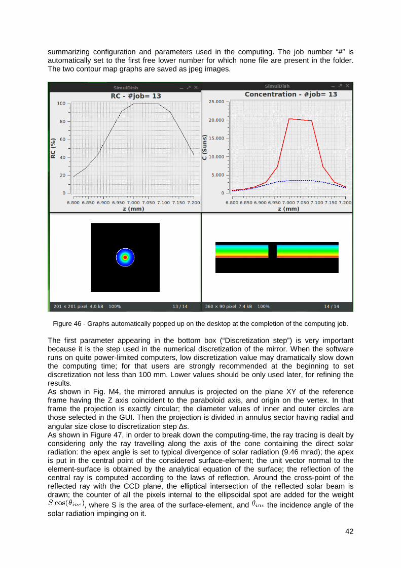
Except the progress bar, the numerical fields contained in the bottom box are filled/refreshed only at the job completion. At the same time four graphs will pop up (see Figure 46): 1) RC versus z, 2) mean and maximum C versus z, 3) flux contour map, and 4) contour map of the incidence angle distribution. In the flux contour map, the window is drawn as a white circle. The numerical data are automatically stored in the “Dish” folder, in the two text files “fluxMap_job_#.txt” and IAD_job_#.txt; the latter is reserved to the incidence angle distribution, the other reports the CCD data achieved at the optimal z, soon after an header
42
summarizing configuration and parameters used in the computing. The job number “#” is automatically set to the first free lower number for which none file are present in the folder. The two contour map graphs are saved as jpeg images.
Figure 46 - Graphs automatically popped up on the desktop at the completion of the computing job.
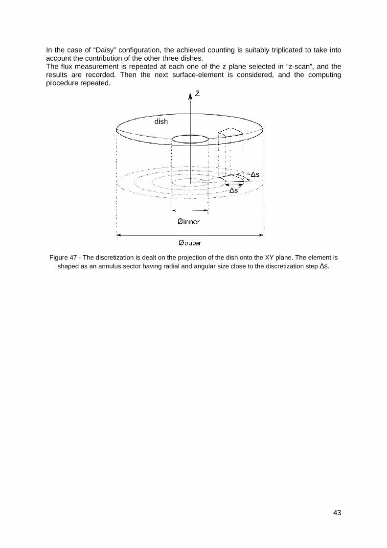
The first parameter appearing in the bottom box (“Discretization step”) is very important because it is the step used in the numerical discretization of the mirror. When the software runs on quite power-limited computers, low discretization value may dramatically slow down the computing time; for that users are strongly recommended at the beginning to set discretization not less than 100 mm. Lower values should be only used later, for refining the results. As shown in Fig. M4, the mirrored annulus is projected on the plane XY of the reference frame having the Z axis coincident to the paraboloid axis, and origin on the vertex. In that frame the projection is exactly circular; the diameter values of inner and outer circles are those selected in the GUI. Then the projection is divided in annulus sector having radial and angular size close to discretization step ∆s. As shown in Figure 47, in order to break down the computing-time, the ray tracing is dealt by considering only the ray travelling along the axis of the cone containing the direct solar radiation: the apex angle is set to typical divergence of solar radiation (9.46 mrad); the apex is put in the central point of the considered surface-element; the unit vector normal to the element-surface is obtained by the analytical equation of the surface; the reflection of the central ray is computed according to the laws of reflection. Around the cross-point of the reflected ray with the CCD plane, the elliptical intersection of the reflected solar beam is drawn; the counter of all the pixels internal to the ellipsoidal spot are added for the weight
, where S is the area of the surface-element, and the incidence angle of the solar radiation impinging on it.
43
In the case of “Daisy” configuration, the achieved counting is suitably triplicated to take into account the contribution of the other three dishes. The flux measurement is repeated at each one of the z plane selected in “z-scan”, and the results are recorded. Then the next surface-element is considered, and the computing procedure repeated.
Figure 47 - The discretization is dealt on the projection of the dish onto the XY plane. The element is
shaped as an annulus sector having radial and angular size close to the discretization step ∆s.
44
Comparison between single and daisy-arrangement of dishes
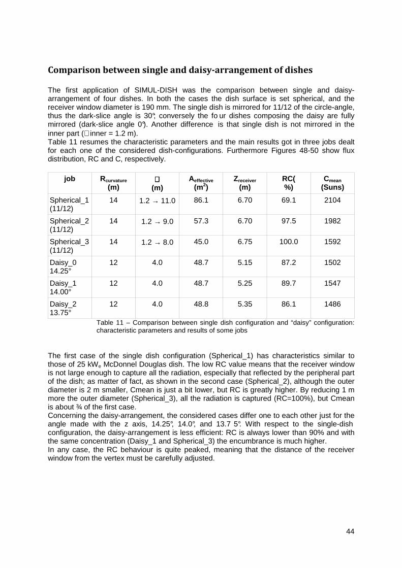
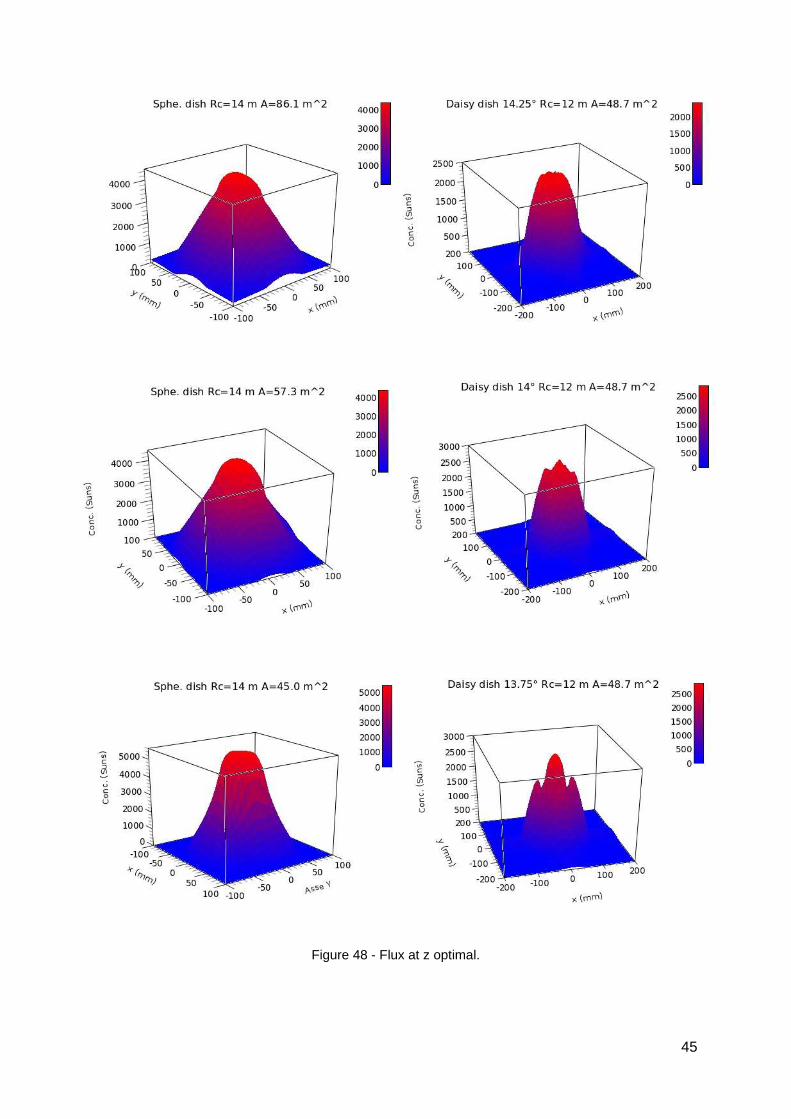
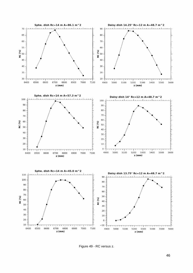
The first application of SIMUL-DISH was the comparison between single and daisy-arrangement of four dishes. In both the cases the dish surface is set spherical, and the receiver window diameter is 190 mm. The single dish is mirrored for 11/12 of the circle-angle, thus the dark-slice angle is 30°; conversely the fo ur dishes composing the daisy are fully mirrored (dark-slice angle 0°). Another difference is that single dish is not mirrored in the inner part (∅inner = 1.2 m). Table 11 resumes the characteristic parameters and the main results got in three jobs dealt for each one of the considered dish-configurations. Furthermore Figures 48-50 show flux distribution, RC and C, respectively.
job Rcurvature (m)
∅∅∅∅ (m)
Aeffective
(m2) Zreceiver
(m) RC( %)
Cmean
(Suns)
Spherical_1 (11/12)
14 1.2 → 11.0 86.1 6.70 69.1 2104
Spherical_2 (11/12)
14 1.2 → 9.0 57.3 6.70 97.5 1982
Spherical_3 (11/12)
14 1.2 → 8.0 45.0 6.75 100.0 1592
Daisy_0 14.25°
12 4.0 48.7 5.15 87.2 1502
Daisy_1 14.00°
12 4.0 48.7 5.25 89.7 1547
Daisy_2 13.75°
12 4.0 48.8 5.35 86.1 1486
Table 11 – Comparison between single dish configuration and “daisy” configuration: characteristic parameters and results of some jobs
The first case of the single dish configuration (Spherical_1) has characteristics similar to those of 25 kWe McDonnel Douglas dish. The low RC value means that the receiver window is not large enough to capture all the radiation, especially that reflected by the peripheral part of the dish; as matter of fact, as shown in the second case (Spherical_2), although the outer diameter is 2 m smaller, Cmean is just a bit lower, but RC is greatly higher. By reducing 1 m more the outer diameter (Spherical_3), all the radiation is captured (RC=100%), but Cmean is about ¾ of the first case. Concerning the daisy-arrangement, the considered cases differ one to each other just for the angle made with the z axis, 14.25°, 14.0°, and 13.7 5°. With respect to the single-dish configuration, the daisy-arrangement is less efficient: RC is always lower than 90% and with the same concentration (Daisy_1 and Spherical_3) the encumbrance is much higher. In any case, the RC behaviour is quite peaked, meaning that the distance of the receiver window from the vertex must be carefully adjusted.
45
Figure 48 - Flux at z optimal.
46
Figure 49 - RC versus z.
47
Figure 50 - Mean and maximum captured concentration versus z.
48
Simulation according to the latest OMSoP project outlining
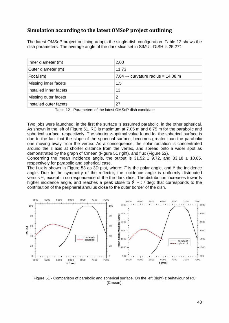
The latest OMSoP project outlining adopts the single-dish configuration. Table 12 shows the dish parameters. The average angle of the dark-slice set in SIMUL-DISH is 25.27°. Inner diameter (m) 2.00
Outer diameter (m) 11.73
Focal (m) 7.04 → curvature radius = 14.08 m
Missing inner facets 1.5
Installed inner facets 13
Missing outer facets 2
Installed outer facets 27 Table 12 - Parameters of the latest OMSoP dish candidate
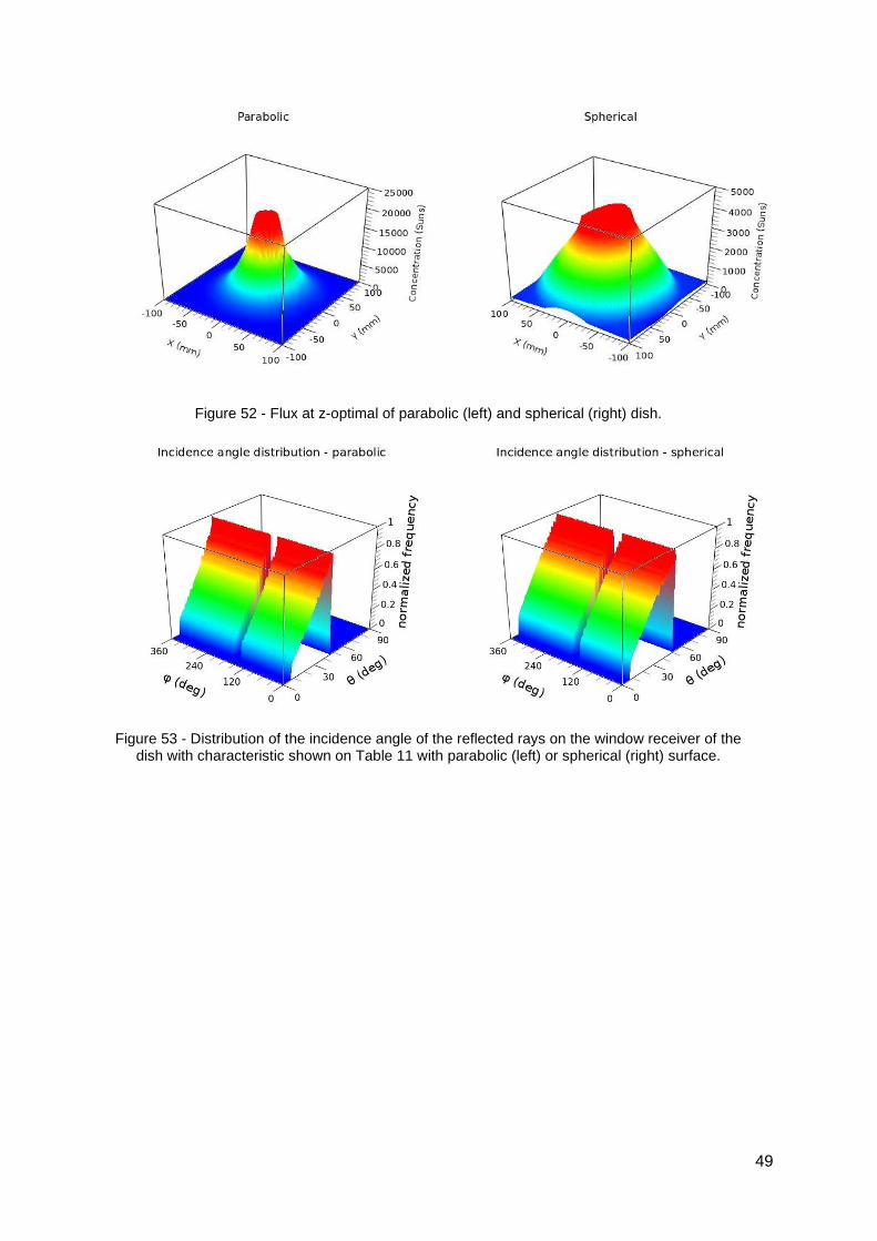
Two jobs were launched; in the first the surface is assumed parabolic, in the other spherical. As shown in the left of Figure 51, RC is maximum at 7.05 m and 6.75 m for the parabolic and spherical surface, respectively. The shorter z-optimal value found for the spherical surface is due to the fact that the slope of the spherical surface, becomes greater than the parabolic one moving away from the vertex. As a consequence, the solar radiation is concentrated around the z axis at shorter distance from the vertex, and spread onto a wider spot as demonstrated by the graph of Cmean (Figure 51 right), and flux (Figure 52). Concerning the mean incidence angle, the output is 31.52 ± 9.72, and 33.18 ± 10.85, respectively for parabolic and spherical case. The flux is shown in Figure 53 as 3D plot, where: is the polar angle, and the incidence angle. Due to the symmetry of the reflector, the incidence angle is uniformly distributed versus , except in correspondence of the the dark slice. The distribution increases towards higher incidence angle, and reaches a peak close to deg; that corresponds to the contribution of the peripheral annulus close to the outer border of the dish.
Figure 51 - Comparison of parabolic and spherical surface. On the left (right) z behaviour of RC (Cmean).
49
Figure 52 - Flux at z-optimal of parabolic (left) and spherical (right) dish.
Figure 53 - Distribution of the incidence angle of the reflected rays on the window receiver of the dish with characteristic shown on Table 11 with parabolic (left) or spherical (right) surface.
50
Wind loads analysis (Adio Miliozzi (ENEA)) Scope of the present work is to evaluate the wind loads acting on the 12m parabolic dish collector (PDC) proposed by Innova for the demonstration task of the project. This type of collector, indeed, is heavily exposed to environmental conditions and, in particular, to the wind actions.
Codes and Standards
Main references, in Europe, to determine the wind actions on a structure are the following Eurocodes [1,2]
• Eurocode 1: Basis of design and actions on structures. Part 2-4: Wind actions, CEN, ENV 1991-2-4, 1994.
• Eurocode 1: Actions on structures - General actions. Part 1-4: Wind actions, CEN, EN 1991- 1-4, 2005.
The Italian codes and standards are directly derived from the previous Eurocodes [3,4]: • Norme tecniche per le costruzioni, D.M. 14 gennaio 2008. • Istruzioni per la valutazione delle azioni e degli effetti del vento sulle costruzioni -
CNR-DT 207/2008 Other references, useful to support this evaluation can be [5,6,7]:
• G. M. Giannuzzi, C. E. Majorana, A. Miliozzi, V.A. Salomoni, D. Nicolini, Structural Design Criteria for Steel Components of Parabolic-Trough Solar Concentrators, Journal of Solar Energy Engineering, NOVEMBER 2007, Vol. 129 / 383
• Miliozzi, G.M. Giannuzzi, D. Nicolini, Valutazione dell’azione del vento su di un concentratore solare parabolico lineare, ENEA Technical Report RT/TER/13/2007
• F. Crobu, Analisi numerica e sperimentale dell’azione del vento su concentratori solari parabolici, Tesi Università di Perugia, 2005
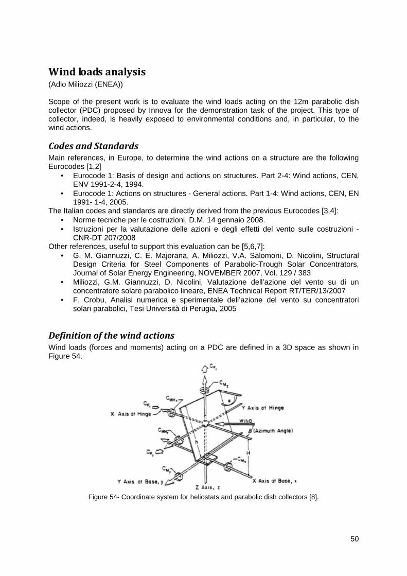
Definition of the wind actions
Wind loads (forces and moments) acting on a PDC are defined in a 3D space as shown in Figure 54.
Figure 54- Coordinate system for heliostats and parabolic dish collectors [8].
51
Wind loads will be evaluated as a function of the peak dynamic pressure of the wind, the main dimension and the aerodynamic coefficients of the PDC in the following way:
AqCF Fxx ⋅⋅=
AqCF Fyy ⋅⋅=
AqCF Fzz ⋅⋅=
DAqCM MHxHx ⋅⋅⋅=
DAqCM MHyHy ⋅⋅⋅=
DAqCM Mzz ⋅⋅⋅=
where D and A are the PDC diameter and aperture area, q is the peak dynamic pressure, C is the aerodynamic coefficient, H is the reference quote of the structure. The peak dynamic pressure q can be calculated, as stated in [1,2,5], as a function of the wind speed, the site characteristics and the reference quote of the structure. The aerodynamic coefficients C are function of the wind direction (β, azimuth angle) and the PDC elevation (α). These coefficients are provided, for common structures, directly by the codes and standards but, for not common structures (our case) they must be evaluated by experimental tests or numerical calculations.
Aerodynamic coefficients: CNR-DT207/2008
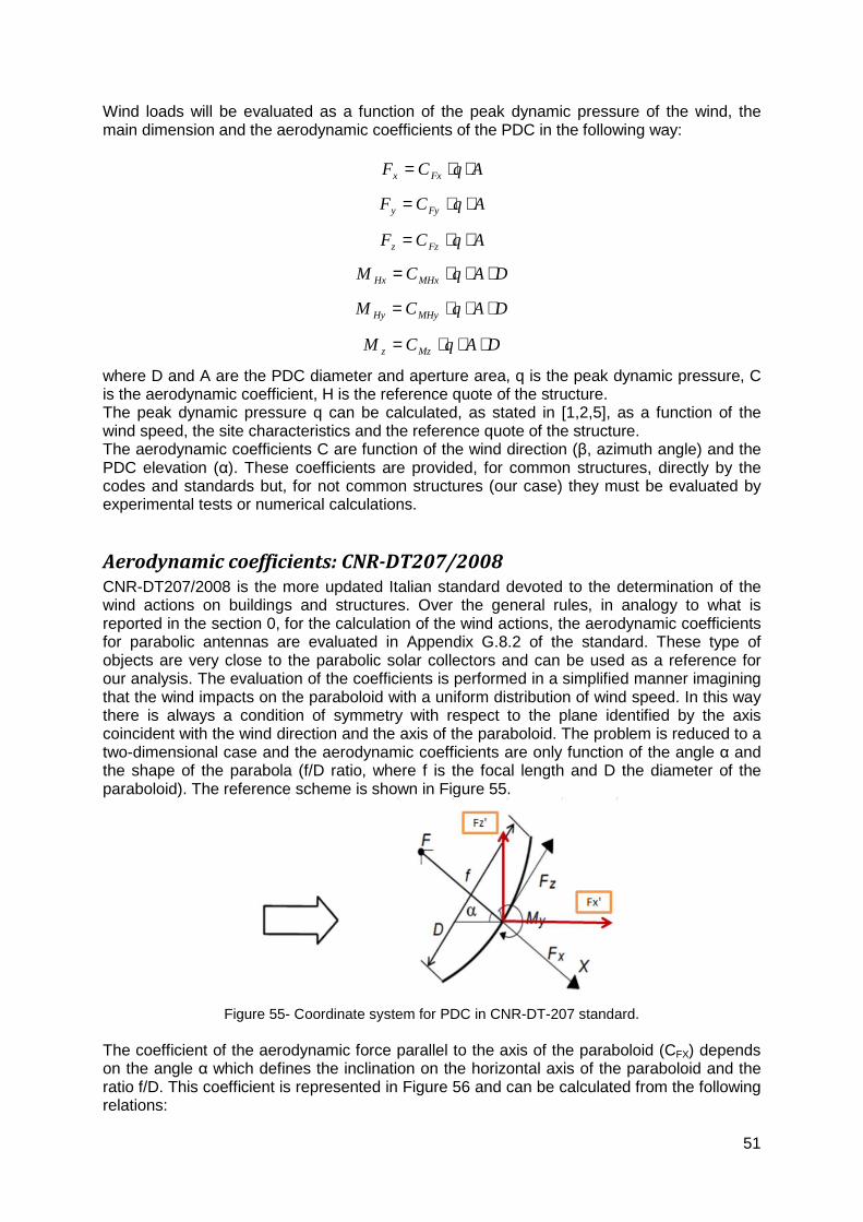
CNR-DT207/2008 is the more updated Italian standard devoted to the determination of the wind actions on buildings and structures. Over the general rules, in analogy to what is reported in the section 0, for the calculation of the wind actions, the aerodynamic coefficients for parabolic antennas are evaluated in Appendix G.8.2 of the standard. These type of objects are very close to the parabolic solar collectors and can be used as a reference for our analysis. The evaluation of the coefficients is performed in a simplified manner imagining that the wind impacts on the paraboloid with a uniform distribution of wind speed. In this way there is always a condition of symmetry with respect to the plane identified by the axis coincident with the wind direction and the axis of the paraboloid. The problem is reduced to a two-dimensional case and the aerodynamic coefficients are only function of the angle α and the shape of the parabola (f/D ratio, where f is the focal length and D the diameter of the paraboloid). The reference scheme is shown in Figure 55.
Figure 55- Coordinate system for PDC in CNR-DT-207 standard.
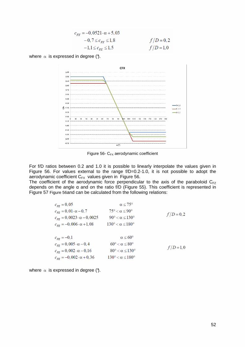
The coefficient of the aerodynamic force parallel to the axis of the paraboloid (CFX) depends on the angle α which defines the inclination on the horizontal axis of the paraboloid and the ratio f/D. This coefficient is represented in Figure 56 and can be calculated from the following relations:
52
where α is expressed in degree (°).
Figure 56- CFX aerodynamic coefficient
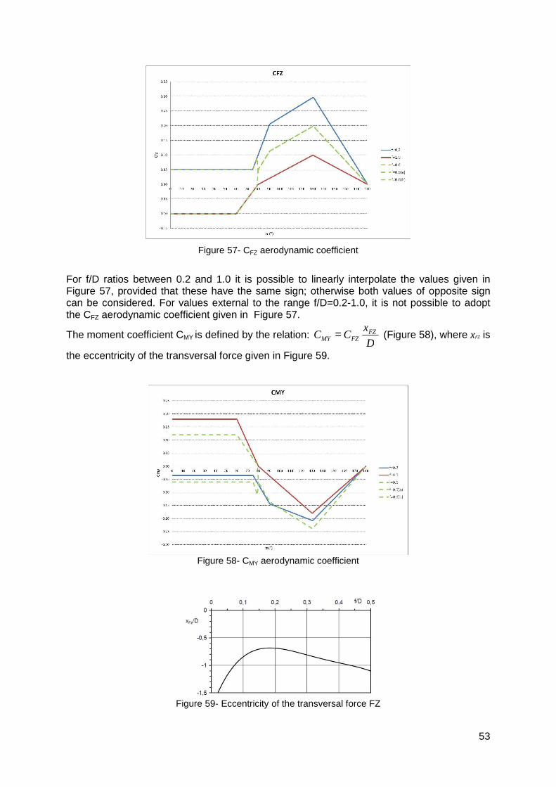
For f/D ratios between 0.2 and 1.0 it is possible to linearly interpolate the values given in Figure 56. For values external to the range f/D=0.2-1.0, it is not possible to adopt the aerodynamic coefficient CFX values given in Figure 56. The coefficient of the aerodynamic force perpendicular to the axis of the paraboloid CFZ depends on the angle α and on the ratio f/D (Figure 55). This coefficient is represented in Figure 57 Figure 56and can be calculated from the following relations:
where α is expressed in degree (°).
53
Figure 57- CFZ aerodynamic coefficient
For f/D ratios between 0.2 and 1.0 it is possible to linearly interpolate the values given in Figure 57, provided that these have the same sign; otherwise both values of opposite sign can be considered. For values external to the range f/D=0.2-1.0, it is not possible to adopt the CFZ aerodynamic coefficient given in Figure 57.
The moment coefficient CMY is defined by the relation: D
xCC FZ
FZMY = (Figure 58), where xFZ is
the eccentricity of the transversal force given in Figure 59.
Figure 58- CMY aerodynamic coefficient
Figure 59- Eccentricity of the transversal force FZ
54
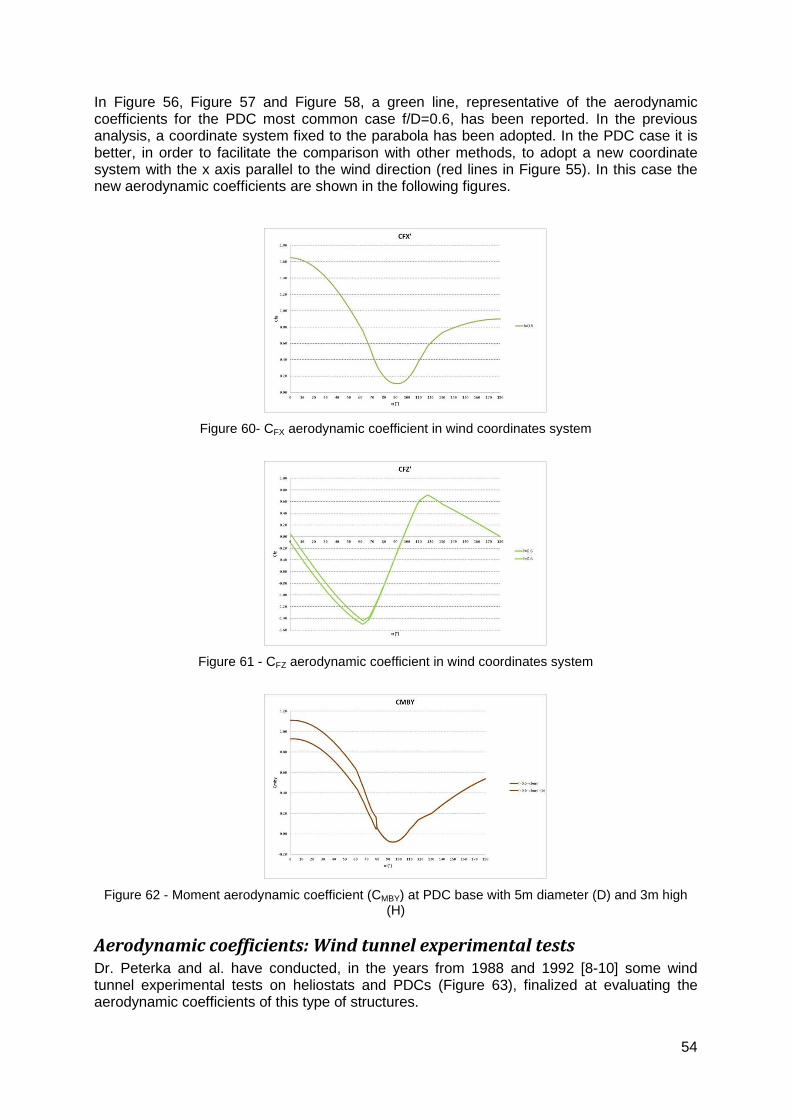
In Figure 56, Figure 57 and Figure 58, a green line, representative of the aerodynamic coefficients for the PDC most common case f/D=0.6, has been reported. In the previous analysis, a coordinate system fixed to the parabola has been adopted. In the PDC case it is better, in order to facilitate the comparison with other methods, to adopt a new coordinate system with the x axis parallel to the wind direction (red lines in Figure 55). In this case the new aerodynamic coefficients are shown in the following figures.
Figure 60- CFX aerodynamic coefficient in wind coordinates system
Figure 61 - CFZ aerodynamic coefficient in wind coordinates system
Figure 62 - Moment aerodynamic coefficient (CMBY) at PDC base with 5m diameter (D) and 3m high
(H)
Aerodynamic coefficients: Wind tunnel experimental tests
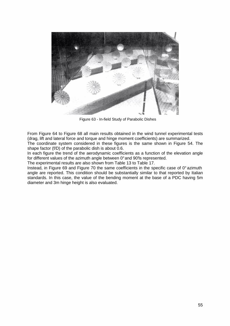
Dr. Peterka and al. have conducted, in the years from 1988 and 1992 [8-10] some wind tunnel experimental tests on heliostats and PDCs (Figure 63), finalized at evaluating the aerodynamic coefficients of this type of structures.
55
Figure 63 - In-field Study of Parabolic Dishes
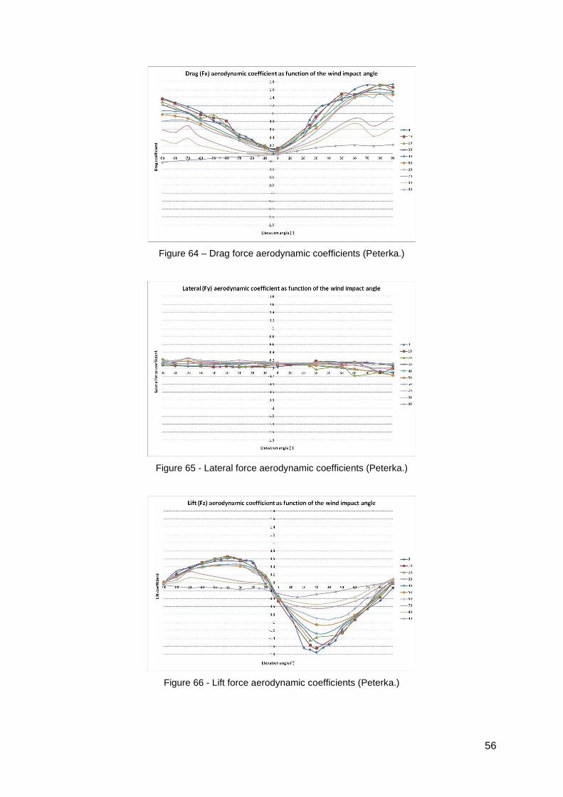
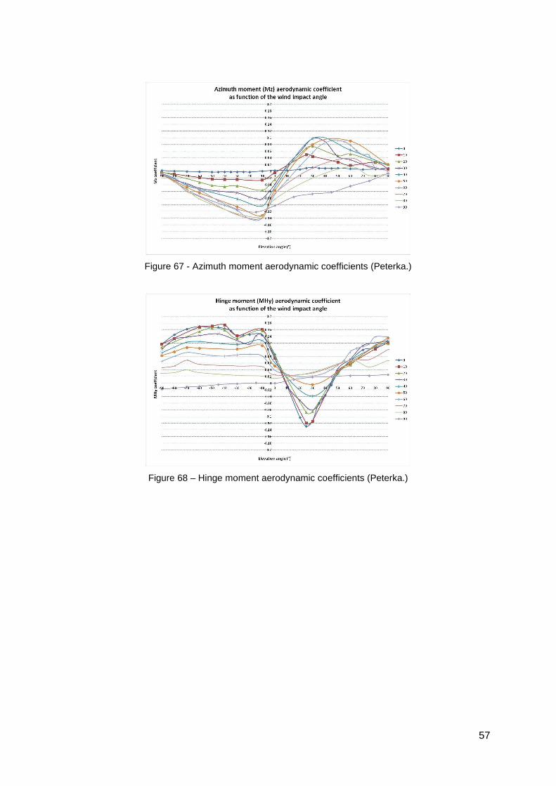
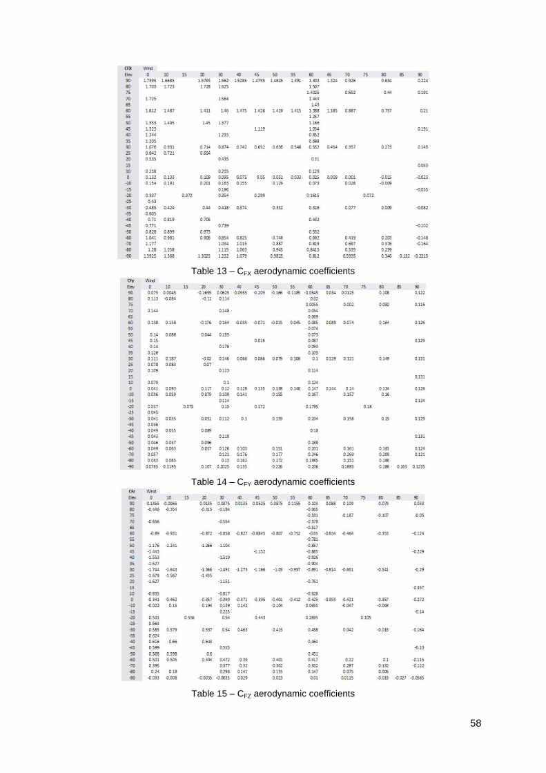
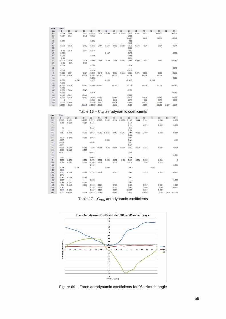
From Figure 64 to Figure 68 all main results obtained in the wind tunnel experimental tests (drag, lift and lateral force and torque and hinge moment coefficients) are summarized. The coordinate system considered in these figures is the same shown in Figure 54. The shape factor (f/D) of the parabolic dish is about 0.6. In each figure the trend of the aerodynamic coefficients as a function of the elevation angle for different values of the azimuth angle between 0° and 90°is represented. The experimental results are also shown from Table 13 to Table 17. Instead, in Figure 69 and Figure 70 the same coefficients in the specific case of 0° azimuth angle are reported. This condition should be substantially similar to that reported by Italian standards. In this case, the value of the bending moment at the base of a PDC having 5m diameter and 3m hinge height is also evaluated.
56
Figure 64 – Drag force aerodynamic coefficients (Peterka.)
Figure 65 - Lateral force aerodynamic coefficients (Peterka.)
Figure 66 - Lift force aerodynamic coefficients (Peterka.)
57
Figure 67 - Azimuth moment aerodynamic coefficients (Peterka.)
Figure 68 – Hinge moment aerodynamic coefficients (Peterka.)
58
Table 13 – CFX aerodynamic coefficients
Table 14 – CFY aerodynamic coefficients
Table 15 – CFZ aerodynamic coefficients
59
Table 16 – CMZ aerodynamic coefficients
Table 17 – CMHy aerodynamic coefficients
Figure 69 – Force aerodynamic coefficients for 0° a zimuth angle
60
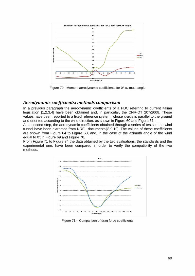
Figure 70 - Moment aerodynamic coefficients for 0° azimuth angle
Aerodynamic coefficients: methods comparison
In a previous paragraph the aerodynamic coefficients of a PDC referring to current Italian legislation [1,2,3,4] have been obtained and, in particular, the CNR-DT 207/2008. These values have been reported to a fixed reference system, whose x-axis is parallel to the ground and oriented according to the wind direction, as shown in Figure 60 and Figure 61. As a second step, the aerodynamic coefficients obtained through a series of tests in the wind tunnel have been extracted from NREL documents [8,9,10]. The values of these coefficients are shown from Figure 64 to Figure 68, and, in the case of the azimuth angle of the wind equal to 0°, in Figure 69 and Figure 70. From Figure 71 to Figure 74 the data obtained by the two evaluations, the standards and the experimental one, have been compared in order to verify the compatibility of the two methods.
Figure 71 – Comparison of drag force coefficients
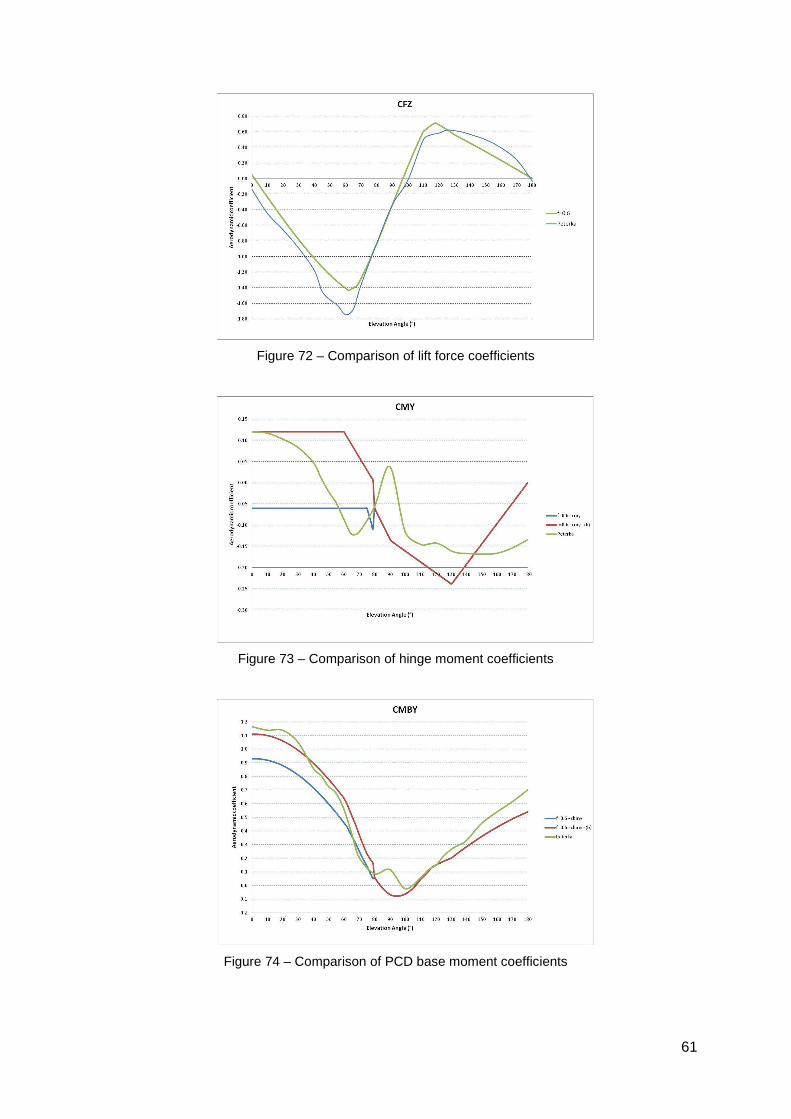
61
Figure 72 – Comparison of lift force coefficients
Figure 73 – Comparison of hinge moment coefficients
Figure 74 – Comparison of PCD base moment coefficients
62
From the analysis of the previous figures it is deducible that:
• The trend of drag and lift coefficients as well as the bending moment at the base of the PDC is very similar for both methods. Instead, the trend related to the coefficient of hinge moment shows significant differences;
• The value of the drag coefficient, calculated according to standard, appears to be quite underestimated for elevations angle above 150°. The same evaluation can be made for the PDC base moment.
From the comparison a substantial equivalence between the two methods emerges even if the differences, especially with regards to the evaluation of the moments, cannot be neglected. This could be due to the actual difference between the objects taken into account. The standards refer to parabolic antennas often installed on buildings and subject to a wind with an uniform velocity distribution. Instead, the experimental tests have simulated PDC installed near the ground and exposed to a distribution of wind with increasing speed (logarithmic) from soil. However, it is necessary to emphasize that, even in the case of moments, the maximum aerodynamic coefficients are coincident, and, then, it is still possible to carry out the evaluation of the peak loads due to the wind. In the following evaluations, the coefficients deri ved from the experimental tests will be taken into account, in consideration of the fact that the tests were carried out in the same conditions as the Innova prototype.
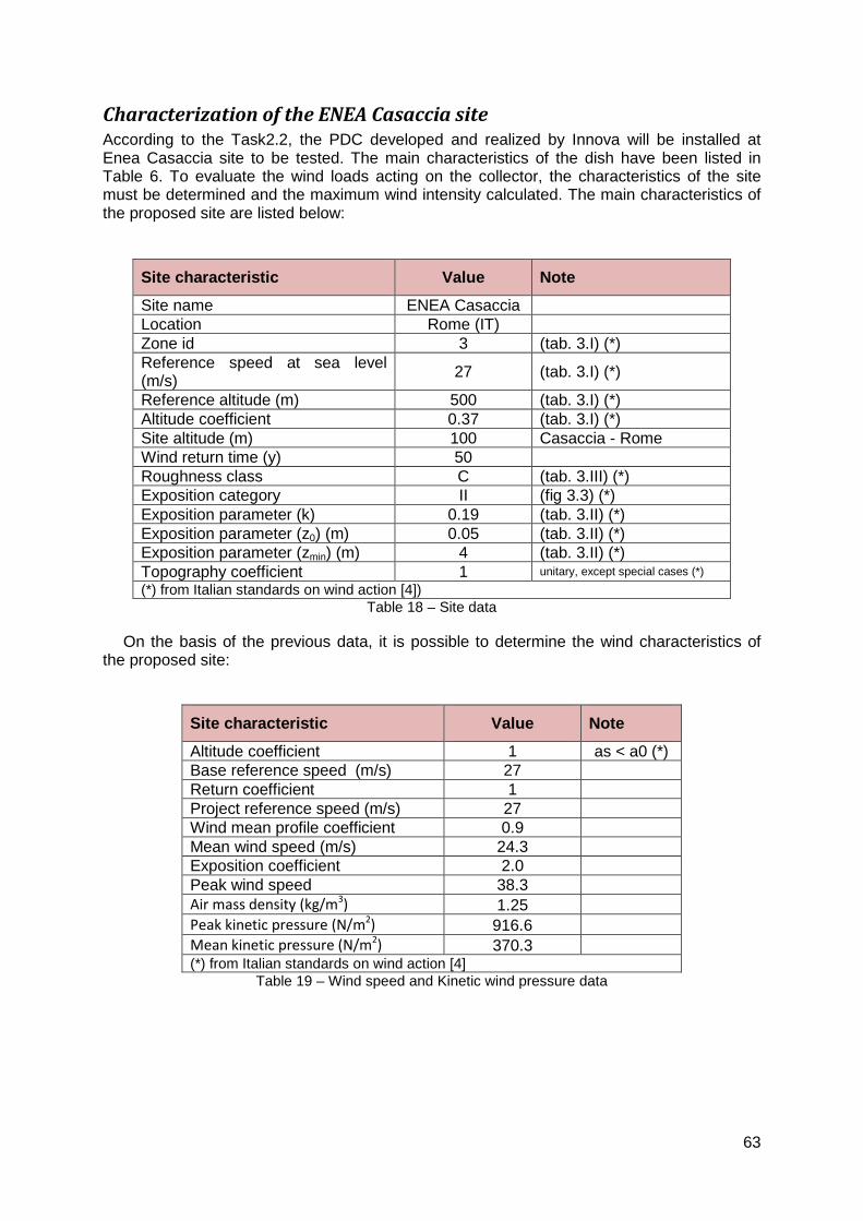
63
Characterization of the ENEA Casaccia site
According to the Task2.2, the PDC developed and realized by Innova will be installed at Enea Casaccia site to be tested. The main characteristics of the dish have been listed in Table 6. To evaluate the wind loads acting on the collector, the characteristics of the site must be determined and the maximum wind intensity calculated. The main characteristics of the proposed site are listed below:
Site characteristic Value Note
Site name ENEA Casaccia Location Rome (IT) Zone id 3 (tab. 3.I) (*) Reference speed at sea level (m/s) 27 (tab. 3.I) (*)
Reference altitude (m) 500 (tab. 3.I) (*) Altitude coefficient 0.37 (tab. 3.I) (*) Site altitude (m) 100 Casaccia - Rome Wind return time (y) 50 Roughness class C (tab. 3.III) (*) Exposition category II (fig 3.3) (*) Exposition parameter (k) 0.19 (tab. 3.II) (*) Exposition parameter (z0) (m) 0.05 (tab. 3.II) (*) Exposition parameter (zmin) (m) 4 (tab. 3.II) (*) Topography coefficient 1 unitary, except special cases (*) (*) from Italian standards on wind action [4])
Table 18 – Site data
On the basis of the previous data, it is possible to determine the wind characteristics of the proposed site:
Site characteristic Value Note
Altitude coefficient 1 as < a0 (*) Base reference speed (m/s) 27 Return coefficient 1 Project reference speed (m/s) 27 Wind mean profile coefficient 0.9 Mean wind speed (m/s) 24.3 Exposition coefficient 2.0 Peak wind speed 38.3 Air mass density (kg/m
3) 1.25
Peak kinetic pressure (N/m2) 916.6
Mean kinetic pressure (N/m2) 370.3
(*) from Italian standards on wind action [4] Table 19 – Wind speed and Kinetic wind pressure data
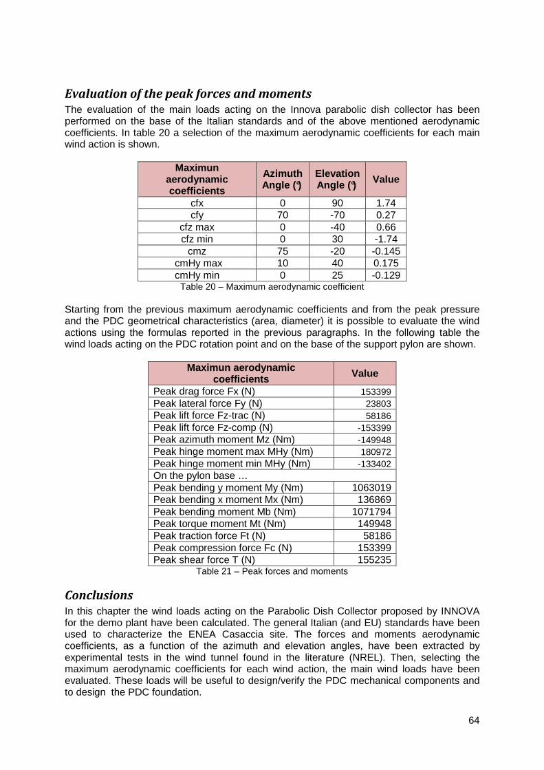
64
Evaluation of the peak forces and moments
The evaluation of the main loads acting on the Innova parabolic dish collector has been performed on the base of the Italian standards and of the above mentioned aerodynamic coefficients. In table 20 a selection of the maximum aerodynamic coefficients for each main wind action is shown.
Maximun aerodynamic coefficients
Azimuth Angle (°)
Elevation Angle (°) Value
cfx 0 90 1.74 cfy 70 -70 0.27
cfz max 0 -40 0.66 cfz min 0 30 -1.74
cmz 75 -20 -0.145 cmHy max 10 40 0.175 cmHy min 0 25 -0.129
Table 20 – Maximum aerodynamic coefficient Starting from the previous maximum aerodynamic coefficients and from the peak pressure and the PDC geometrical characteristics (area, diameter) it is possible to evaluate the wind actions using the formulas reported in the previous paragraphs. In the following table the wind loads acting on the PDC rotation point and on the base of the support pylon are shown.
Maximun aerodynamic coefficients Value
Peak drag force Fx (N) 153399 Peak lateral force Fy (N) 23803 Peak lift force Fz-trac (N) 58186 Peak lift force Fz-comp (N) -153399 Peak azimuth moment Mz (Nm) -149948 Peak hinge moment max MHy (Nm) 180972 Peak hinge moment min MHy (Nm) -133402 On the pylon base … Peak bending y moment My (Nm) 1063019 Peak bending x moment Mx (Nm) 136869 Peak bending moment Mb (Nm) 1071794 Peak torque moment Mt (Nm) 149948 Peak traction force Ft (N) 58186 Peak compression force Fc (N) 153399 Peak shear force T (N) 155235
Table 21 – Peak forces and moments
Conclusions
In this chapter the wind loads acting on the Parabolic Dish Collector proposed by INNOVA for the demo plant have been calculated. The general Italian (and EU) standards have been used to characterize the ENEA Casaccia site. The forces and moments aerodynamic coefficients, as a function of the azimuth and elevation angles, have been extracted by experimental tests in the wind tunnel found in the literature (NREL). Then, selecting the maximum aerodynamic coefficients for each wind action, the main wind loads have been evaluated. These loads will be useful to design/verify the PDC mechanical components and to design the PDC foundation.
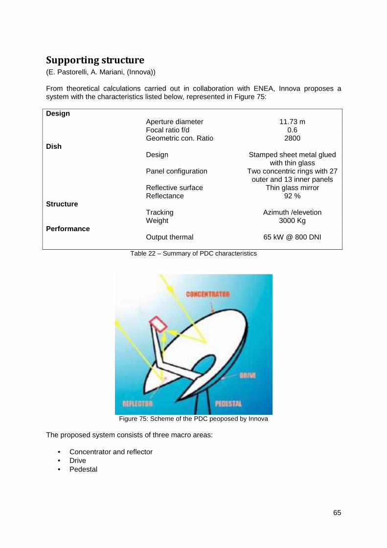
65
Supporting structure (E. Pastorelli, A. Mariani, (Innova)) From theoretical calculations carried out in collaboration with ENEA, Innova proposes a system with the characteristics listed below, represented in Figure 75: Design Aperture diameter 11.73 m Focal ratio f/d 0.6 Geometric con. Ratio 2800 Dish Design Stamped sheet metal glued
with thin glass Panel configuration Two concentric rings with 27
outer and 13 inner panels Reflective surface Thin glass mirror Reflectance 92 % Structure Tracking Azimuth /elevetion Weight 3000 Kg Performance Output thermal 65 kW @ 800 DNI
Table 22 – Summary of PDC characteristics
Figure 75: Scheme of the PDC peoposed by Innova
The proposed system consists of three macro areas:
• Concentrator and reflector • Drive • Pedestal
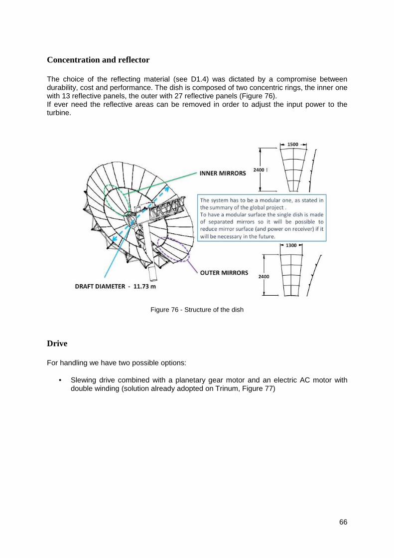
66
Concentration and reflector The choice of the reflecting material (see D1.4) was dictated by a compromise between durability, cost and performance. The dish is composed of two concentric rings, the inner one with 13 reflective panels, the outer with 27 reflective panels (Figure 76). If ever need the reflective areas can be removed in order to adjust the input power to the turbine.
Figure 76 - Structure of the dish
Drive For handling we have two possible options:
• Slewing drive combined with a planetary gear motor and an electric AC motor with double winding (solution already adopted on Trinum, Figure 77)
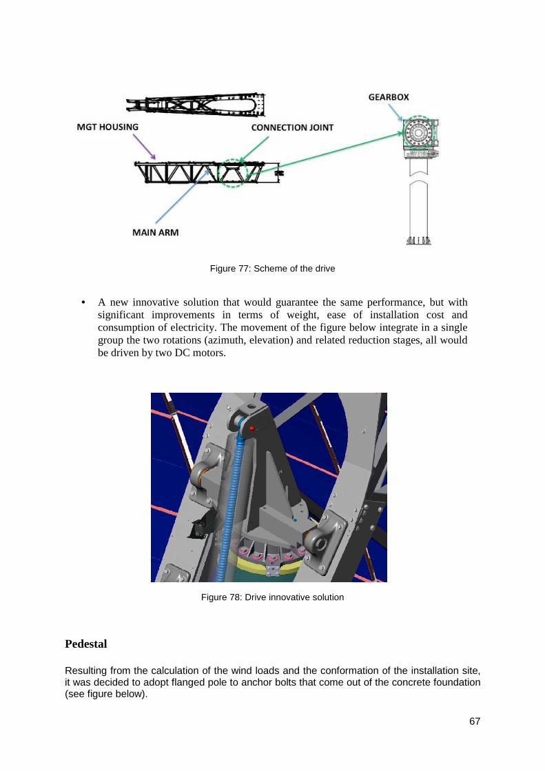
67
Figure 77: Scheme of the drive
• A new innovative solution that would guarantee the same performance, but with significant improvements in terms of weight, ease of installation cost and consumption of electricity. The movement of the figure below integrate in a single group the two rotations (azimuth, elevation) and related reduction stages, all would be driven by two DC motors.
Figure 78: Drive innovative solution
Pedestal Resulting from the calculation of the wind loads and the conformation of the installation site, it was decided to adopt flanged pole to anchor bolts that come out of the concrete foundation (see figure below).
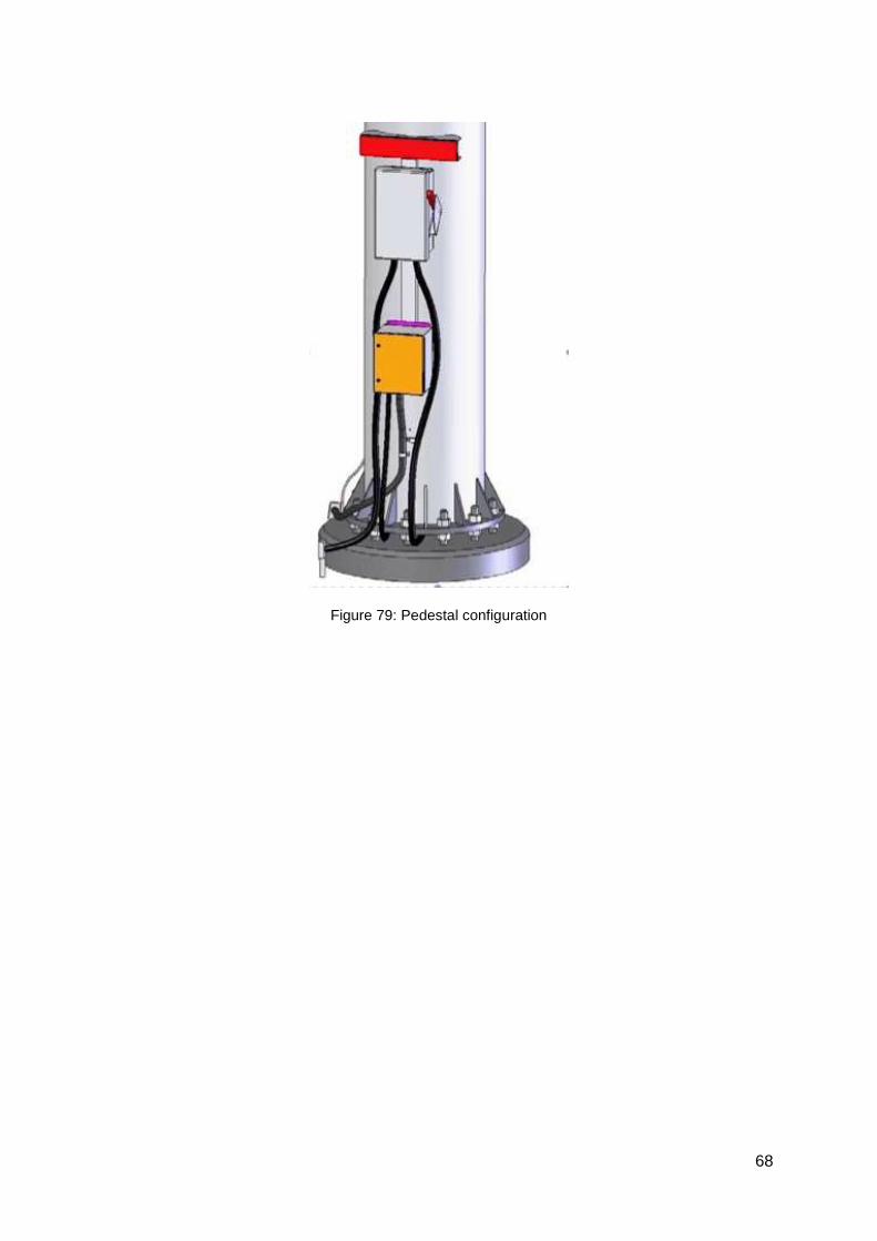
68
Figure 79: Pedestal configuration
69
Tracking system specifications (E. Pastorelli, A. Mariani (Innova)) SunTrinum is a complete system for the two-axis solar tracking by the astronomical calculation of the equations that govern the motion of the earth relative to the sun. All information necessary for the operation are detected by an integrated GPS receiver. After the first installation, the system will be completely autonomous since the parameters involved in the operation and configuration of the system are resident in flash memory and protected by a security password. The interaction of the system with the operator is assigned to a graphic display 128x64 pixels flanked by 5 buttons. The current SunTrinum unit will be adapted to the new system in terms of hardware (encoder, dc electric motor, wind and rain sensor), and also in the firmware (the firmware will be rewritten to optimize the needs of the machine). The control unit will also be adapted so that it can interact with the control center of ENEA. Below some particularities of the control unit are reported. Calculating solar coordinates The main function of SunTrinum is to calculate the position of the sun (in azimuth and elevation ) being known the exact time and terrestrial coordinates of the place of installation. This information is automatically received by the GPS receiver (Global Positioning System) integrated in KS150, allowing a high degree of automation of the system. Using the GPS , in fact, it is possible to know the exact location of solar tracking system (in terms of latitude, longitude and dial) and the exact time of the astronomical given time. Based on these parameters the position of the sun on the horizon in terms of azimuth and elevation can be calculated with absolute precision, to ensure effective tracking of the star. The autonomy of the system is completed by a rain and wind sensor, that provide additional details on the meteorological conditions, and consequently, the efficiency of the system. The tracker turns out to be totally independent in its actions of pointing, and in the ability to assess the overall energy balance. The calculated values of azimuth and elevation of the sun are shown in real time on the main screen, along with the date and time zone. Regarding the display of the date and time a parameter is of particular importance: Timezone. It identifies the time zone membership increased by 12 hours. For example, since in Italy the time zone is +1, the value to be entered in parameter is 13. Operation mode There are three modes of operation: manual, automatic and safe location. 1) Manual: The system can be set by the operator using the four buttons ▲, ▼, ◄, ► (Up, Down, Left, Right). This mode is used during maintenance and to move the dish to taste and to make the first zero of the system; 2) Automatic: The system begins to chase the sun independently, on the base of data calculated by the internal equioment;

70
3) Safe: The system places the parabola closed down on itself (see parameters AziSafe and ElevSafe) and remains there until the operator decides to put the system back manually or automatically, by pressing the menu. This mode finds its main use in the process of installation and maintenance. Daily cycle The system becomes fully operational by setting it in automatic mode. The sleep position is intented to be the configuration of the parabola having azimuth value equal to the value indicated by AziSleep and elevation equal to the value indicated by ElevSleep, expressed in degrees to be considered negative . The position is reached in the evening, when, considering the position of the sun, the system decides to stop the pursuit and wait for the dawn of the next day. The safe position is used to bring the dish in security (in case of power failure, wind or rain ) and can be set manually by placing the system in safe mode (Menu → Mode → Safe Mode ) The daily cycle begins in the morning, when the system detects that the amount of elevation of the sun is above WakeupElev, expressed in degrees: the parabola comes out from the rest position and from then on begins to chase the sun . Similarly, during the afternoon, the system returns to the rest position when the height of the sun is lowered below the portion SleepElev, expressed in degrees. These two parameters are useful to stop the tracking of the sun when this is too close to the horizon in order to provide sufficient energy, in this case the handling would be counterproductive. Refer to the height of the sun rather than to a fixed schedule allows you to have optimal behavior in any season. For only demonstration purposes, it is possible to simulate the daily movement of the virtual parabola increasing the speed tracking of the sun. The value of the parameter SimulSun indicates the multiplication factor of acceleration of the movement. For example, setting it to 60 per second is equivalent to a real movement of the sun for a minute, then a daily cycle 60 times shorter (the cycle will end in 24 minutes). This parameter must be 0 for the proper functionality of the system. Conditions external to the system The system, via sensors, continuously detects the presence of electric network and the possible presence of rain or wind. Presence of grid. The system is able to detect the presence of electrical network and it can distinguish whether it is powered directly from the grid or via the UPS group. In case of absence of the mains voltage, the parabola will continue to chase the sun for the time indicated by the parameter FltGridOn. After that the system will bring in safe position , not to consume too much battery pending restoration of the network. Rain sensor. If the sensor detects the presence of rain for a number of seconds at least equal to the value specified by the parameter FltRainOn, the system goes into safe location . After the rain , the system waits for a number of seconds equal to the value specified by the parameter FltRainOff before returning to chase the sun . Wind speed sensor. If, for a number of seconds at least equal to the value specified by the parameter FltWindOn, it is detected wind speed greater than the value specified by the
71
parameter MaxWindSpd, expressed in km/h , the system goes into safe position to avoid mechanical damage. Before returning to chase the sun, the system waits for a number of minutes equal to the value specified by the parameter FltWindOff .
References
[1] Eurocode 1: Basis of design and actions on structures. Part 2-4: Wind actions, CEN, ENV 1991-2-4, 1994.
[2] Eurocode 1: Actions on structures - General actions. Part 1-4: Wind actions, CEN, EN 1991- 1-4, 2005.
[3] Norme tecniche per le costruzioni, D.M. 14 Gen 2008.
[4] Istruzioni per la valutazione delle azioni e degli effetti del vento sulle costruzioni - CNR-DT 207/2008
[5] G. M. Giannuzzi, C. E. Majorana, A. Miliozzi, V.A. Salomoni, D. Nicolini, Structural Design Criteria for Steel Components of Parabolic-Trough Solar Concentrators, Jnl of Solar Energy Engineering, Vol. 129 Nov. 2007 pp 382-390
[6] A. Miliozzi, G.M. Giannuzzi, D. Nicolini, Valutazione dell’azione del vento su di un concentratore solare parabolico lineare, ENEA Technical Report RT/TER/13/2007
[7] F. Crobu, Analisi numerica e sperimentale dell’azione del vento su concentratori solari parabolici, Thesis, Perugia University, 2005
[8] J.A. Peterka, R.G. Derickson, Wind load design methods for heliostats and parabolic dish collectors, Sand92-7009, Sep 1992
[9] J.A. Peterka, R.G. Derickson, J.E. Cermak, Wind loads and local pressure distributions on parabolic dish collectors, Seri/TP-253-3668, May 1990
[10] J.A. Peterka, Z. Tan, B. Bienkiewicz, J.E. Cermak, Wind loads on heliostats and parabolic dish collectors, Seri/STR-253-3431, Nov 1988


![TMHFR FR BT Optio Family [749630-040] Brochure_low Res](https://img.pdfslide.us/doc/110x75/577c7a751a28abe054954820/tmhfr-fr-bt-optio-family-749630-040-brochurelow-res.jpg)