Embed Size (px)
Citation preview

Grant Agreement: 644047
INtegrated TOol chain for model-based design of CPSs
D1.2- Case Studies 2
Deliverable Number: D1.2
Version: 1.0
Date: 11 2016
Public Document
http://into-cps.au.dk

D1.2 - Case Studies 2 (Public)
Contributors:
Julien Ouy, CLEThierry Lecomte, CLEMartin Peter Christiansen, AIAndres Vill Henriksen, AIOle Green, AIStefan Hallerstede, AUPeter Gorm Larsen, AUClaes Jger, AIStylianos Basagiannis, UTRCLuis Diogo Couto, UTRCAlie El-din Mady, UTRCHassan Ridouanne, UTRCHector Moner Poy, UTRCJuan Valverde Alcala, UTRCChristian Konig, TWTNatalia Balcu, TWT
Editors:
Julien Ouy, CLE
Reviewers:
Simon Foster, UYChristian Kleijn, CLPStefan Hallerstede, AU
Consortium:
Aarhus University AU Newcastle University UNEWUniversity of York UY Linkoping University LIUVerified Systems International GmbH VSI Controllab Products CLPClearSy CLE TWT GmbH TWTAgro Intelligence AI United Technologies UTRCSofteam ST
2

D1.2 - Case Studies 2 (Public)
Document History
Ver Date Author Description0.1 06-15-2016 JO Initial document version0.2 07-06-2016 JO CPS aspects of the use cases0.3 08-25-2016 JO first version of the CLE use case0.4 08-30-2016 MPC addition of the AI use case0.5 10-25-2016 JO addition of the complementarity table0.6 10-28-2016 MPC update of the AI use case0.7 10-31-2016 CK addition of the TWT use case0.8 11-04-2016 SB addition of the UTRC use case0.9 11-08-2016 JO internal review version1.0 11-30-2016 JO corrections following internal review1.0 12-16-2016 JO final version
3

D1.2 - Case Studies 2 (Public)
This document shows the four industrial partners’ case studies. A case studycontains the description of the industrial case, the modelling and simulation of itusing INTO-CPS baseline tools and the assessment of the baseline tools accord-ing to their requirements. The goal of this deliverable is to bring insights aboutindustrial benefits and weaknesses of using INTO-CPS baseline tools.
Contents1 Introduction 6
2 Cyber-Physical aspects of the Industrial Case Studies 62.1 Cyber-Physical aspects of the Railway case study . . . . . . . . . 62.2 Cyber-Physical aspects of the Agriculture case study . . . . . . . 72.3 Cyber-Physical aspects of the Building case study . . . . . . . . . 82.4 Cyber-Physical aspects of the Automobile case study . . . . . . . 82.5 Complementarity of the Industrial Case Studies . . . . . . . . . . 102.6 Key Performance Indicators . . . . . . . . . . . . . . . . . . . . 10
3 Railway case study 113.1 The Case study . . . . . . . . . . . . . . . . . . . . . . . . . . . 113.2 Contribution during Year 2 . . . . . . . . . . . . . . . . . . . . . 153.3 Industrial needs and assessments . . . . . . . . . . . . . . . . . . 23
4 Agriculture Case Study 344.1 Introduction . . . . . . . . . . . . . . . . . . . . . . . . . . . . . 344.2 Agriculture case study . . . . . . . . . . . . . . . . . . . . . . . 344.3 Modelling . . . . . . . . . . . . . . . . . . . . . . . . . . . . . . 394.4 Robotti Second Generation . . . . . . . . . . . . . . . . . . . . . 454.5 Industrial needs and assessment . . . . . . . . . . . . . . . . . . 49
5 Building Case Study 565.1 Introduction . . . . . . . . . . . . . . . . . . . . . . . . . . . . . 565.2 Building Case Study . . . . . . . . . . . . . . . . . . . . . . . . 565.3 Modeling . . . . . . . . . . . . . . . . . . . . . . . . . . . . . . 585.4 HVAC Co-simulation Results . . . . . . . . . . . . . . . . . . . . 665.5 Industrial Needs and Assessment . . . . . . . . . . . . . . . . . . 685.6 UTRC-Req-001: Simulation Completeness . . . . . . . . . . . . 695.7 UTRC-Req-002: Simulation Delays . . . . . . . . . . . . . . . . 695.8 UTRC-Req-003: Design Space Exploration . . . . . . . . . . . . 705.9 UTRC-Req-004: Simulation Accuracy and Precision . . . . . . . 70
4

D1.2 - Case Studies 2 (Public)
5.10 UTRC-Req-005: Scalable Simulation . . . . . . . . . . . . . . . 715.11 UTRC-Req-006: Code generation . . . . . . . . . . . . . . . . . 715.12 UTRC-Req-007: Platform Independence and FMU support . . . . 725.13 Conclusion - Reporting Experiences . . . . . . . . . . . . . . . . 72
6 Automotive Case Study 746.1 Specifications . . . . . . . . . . . . . . . . . . . . . . . . . . . . 746.2 Specification of the HiL scenario . . . . . . . . . . . . . . . . . . 766.3 Model . . . . . . . . . . . . . . . . . . . . . . . . . . . . . . . . 786.4 Route module (CT) . . . . . . . . . . . . . . . . . . . . . . . . . 806.5 Alarm System (DE) . . . . . . . . . . . . . . . . . . . . . . . . . 806.6 Simulation results . . . . . . . . . . . . . . . . . . . . . . . . . . 806.7 Evaluation of INTO-CPS tools . . . . . . . . . . . . . . . . . . . 826.8 Requirements and Assessments . . . . . . . . . . . . . . . . . . . 856.9 Conclusion . . . . . . . . . . . . . . . . . . . . . . . . . . . . . 89
5
D1.2 - Case Studies 2 (Public)
1 Introduction
This document shows the four industrial partners case studies: the Railway casestudy from CLE, the Agriculture case study from AI, the Building case study fromUTRC and the the Automative case study from TWT. Each case study containsthe public description of the industrial case, the modelling and simulation of itusing INTO-CPS baseline tools and the assessment of the baseline tools accordingto their requirements. Prior to the descriptions of the case studies, a section isdedicated to specific points addressed during the first year of the project, the cyber-physical aspects of the case-studies.
2 Cyber-Physical aspects of the Industrial Case Stud-ies
Each of the case-studies presents in a different angle the aspects of a Cyber-physical system. Individually they only cover a fraction of the different featuresthat characterize a CPS but altogether the case studies of INTO-CPS demonstrateall that can be modeled, checked, tested, simulated or generated using the toolsprovided by INTO-CPS.
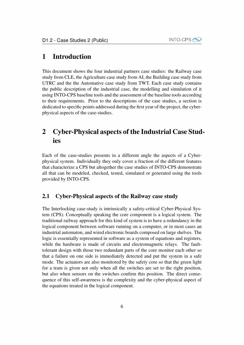
2.1 Cyber-Physical aspects of the Railway case study
The Interlocking case-study is intrinsically a safety-critical Cyber-Physical Sys-tem (CPS). Conceptually speaking the core component is a logical system. Thetraditional railway approach for this kind of system is to have a redundancy in thelogical component between software running on a computer, or in most cases anindustrial automaton, and wired electronic boards composed on large shelves. Thelogic is essentially represented in software as a system of equations and registers,while the hardware is made of circuits and electromagnetic relays. The fault-tolerant design with those two redundant parts of the core monitor each other sothat a failure on one side is immediately detected and put the system in a safemode. The actuators are also monitored by the safety core so that the green lightfor a tram is given not only when all the switches are set to the right position,but also when sensors on the switches confirm this position. The direct conse-quence of this self-awareness is the complexity and the cyber-physical aspect ofthe equations treated in the logical component.
6

D1.2 - Case Studies 2 (Public)
The Interlocking case study focus on an innovation which add yet another cyber-physical element: the distribution of the system over several simple modules,which is considered a challenge for the traditional railway industry. Whereasit can be simple to prove that each module has the same local safety level as acentralized interlocking the fact that a module allows a route only when it is safeto the knowledge of its own sensors is challenging to argue for. It is significantlymore difficult to demonstrate safety at the global level because protocols and net-works intervene in the challenge. Yet an innovative distributed Interlocking wouldhave benefits for the industry with simpler hardware and the possibility to reachnew markets where the distance or the complexity of the geography would preventthe use of a classical system.
The use of heterogeneous models with co-simulation and/or model checking wouldalso lower the time to market of such a product. In railways safety, systems arerarely Commercial of the shelf, since a large part of adaptation and parameteriza-tion are needed before it is possible to deliver the final product. Moreover, duringthe installation, the system or the equipment interacting with it are not necessar-ily available for testing purposes or not truely representative of the final system.For those reasons, reasoning and testing with a model-based representation of thesystem as carried out in the INTO-CPS project can be seen as a major cost saverin being able to test in a virtual setting before one have to go into an expensiveseries of physical tests.
2.2 Cyber-Physical aspects of the Agriculture case study
The agricultural robot platform is comprised of a network of interacting computerunits that operate with inputs from and provide outputs to its physical environ-ment. The physical environment the agricultural robot platform is operating inis influenced by geography, weather and terrain conditions. The robot platformis a mobile CPS that needs to incorporate concepts from multiple engineeringdisciplines such as agricultural, control, electrical, mechanical, signal processingand software design. The robot needs to be able to operate autonomously withminor levels of human surveillance, so it needs to have its own “intelligence”.Thus, this system has a high degree of autonomy. Dramatic changes have beenmade to the overall system engineering design of the Robotti platform, and thusfrom a commercial perspective it is definitely advantageous to be able to carryout initial investigations in a virtual setting instead of wasting too much time andmoney on producing full-scale expensive physical prototypes. These aspects col-lectively make the agricultural case study a good example of a CPS in the INTO-CPS project.
7

D1.2 - Case Studies 2 (Public)
2.3 Cyber-Physical aspects of the Building case study
The building case study is considered to be a full CPS, composed by several cyberand physical elements. The cyber part of the year 2 case study include compo-nents such as the FCU controllers that will be embedded in the hardware devices,the communication interfaces in order to handle communication locally betweenthe FCUs and globally between the FCUs and the supervisor. Communicationmodules will also coexist within the same FCU hardware device and will han-dle distributed communications exchanged between the FCUs and the supervi-sor. Commands for both the controllers and communications modules will handleswitching mechanisms for certain FCU elements that include the device itself (e.g.on), regulating the fan speed (e.g. medium speed), regulating the air-dumper po-sition (e.g. 10% open), regulating the power of the coil (e.g. 20V) and regulatingthe water valves position (e.g. 50% open). The aforementioned elements will betargeted for code generation in order to proceed with Software-in-the-Loop andHardware-in-the-Loop simulations for the aforementioned case study. Finally thecommunication medium used in the HVAC CPS scenario is also based on pro-tocol message exchange between the supervisor and the FCU controllers (e.g.through UART). The physical part of the year 2 case study will include compo-nents that will be co-modeled with the cyber part in the multi-models evaluated inthe INTO-CPS platform. Those components include the thermal modeling of thephysical rooms and zones in order to study thermal affects of the areas includingwall insulation parameters and air-mass heat capacity. Air pipes connection andair flow exchanged between the Air Handling Unit (AHU) and the FCUs is alsocontinuously described by air mass flow inside the pipes used in the building toconnect the AHU and the FCUs. Water pipes connection and water flow pressureexchanged between the Heat Pump Unit the FCUs and the AHU, is also governedby continuous equations describung fluid dynamics in the water pipes, pressurizedin the Heat Pump and heated or colling at the AHU towards the FCUs. Currentcontinuous models includes 21.000 variables with a total of 11.000 parameters,while the number of differential equations used to describe the system dynamicsis close to 7000.
2.4 Cyber-Physical aspects of the Automobile case study
The automotive case study can be considered a Cyber-Physical-System (CPS) be-cause it contains local intelligence and autonomy in the vehicle. This is assistedby information about its environment typically derived from a cloud context (here,information on weather and traffic / route) and the logic depends upon the physicaldynamics of the electric vehicle. In the most innovative scenario that is described
8

D1.2 - Case Studies 2 (Public)
in section 6.2, a real driver is able to drive a simulated vehicle (using a virtual re-ality environment). Here the characteristic curve of the accelerator (gas pedal) isadapted based on the remaining range of the vehicle enabled by its battery. If therange is too low for reaching the designated destination, the curve will be ”soft-ened”, resulting in less acceleration at a given position of the accelerator. Thecontroller that changes this characteristic curve is inherently a cyber element (acontroller, running for example on a Raspberry Pi), which interacts with the phys-ical world (the human driver and the vehicle’s dynamics, which is modeled). Thiscontroller is developed using the INTO-CPS tool chain and its methodology, froma systems engineering perspective. Thus, the different constituent elements of thesystem can be analysed using the HiL capability, as well as features such as test-ing and code generation that are covered by the INTO-CPS tool chain. Since theCo-Simulation that is used to determine the remaining range of the electric vehi-cle, also uses information from its environment (route and weather information),it can be considered a smart connected system. At the time of writing, the HiLscenario is being designed, and its implementation is planned for year 3.
9

D1.2 - Case Studies 2 (Public)
2.5 Complementarity of the Industrial Case Studies
The table 1 summarises the different aspects of CPS and the related major indus-trial needs covered by the case studies of INTO-CPS. Parenthesized yes meansthat the feature is present in the case study but not completely implemented yet.We see that except for size efficiency, all aspects appear in one or more case stud-ies. Some of them, mainly formal verification, design test exploration and testautomation are to be explored in Y3.
Table 1: Complementarities of the industrial case studies at Y2
Application area Railways Agriculture Buildings AutomotiveLead partner CLE AI UTRC TWTTime Critical Yes (Yes) Yes NoSafety Critical Yes (Yes) No NoAutonomy Yes Yes Yes YesPower efficiency No No YesHigh Performance Yes (Yes) Yes YesSize Efficiency No No No NoCost efficiency Yes Yes Yes NoActuators modeling Yes Yes (Yes) YesSensors modeling Yes Yes Yes YesNetwork modeling Yes (Yes) (Yes) (Yes)Formal verification (Yes) No Yes NoSIL Co-simulation Yes Yes (Yes) (Yes)HIL Co-Simulation Yes Yes No (Yes)Design Space Explo-ration
No Yes (Yes) (Yes)
Test-Automation (Yes) No No (Yes)
2.6 Key Performance Indicators
Key performance concerning WP1 relies on three indicators.
KPI-A, utility assessment We can affirm that this indicators has been reached,all case studies in Y2 are developed following the methods and tools from Into-CPS: development of SYS-ML models, CT and DE models of the different com-ponents, generation of FMU from Overture, OpenModelica or 20-sim, executionof co-simulation with the COE. This will be detailed in this document.
10

D1.2 - Case Studies 2 (Public)
KPI-B, Reduction of development time for CPS This indicator is evaluatedindirectly and has to be detailed for each case study. For CLE we can cite theearly evaluation of the safety properties of the system that saved a lot of time:several propositions of distribution have been created and tested for safety prop-erties as models, this phase could append before the choice of the hardware andthe development of drivers or communication layers (middleware). This saved thetime and money of developing several module prototypes. In the second phase,when the prototype has been tested, no reason came for questioning the choice ofthe distribution and requiring a second iteration. Automatic code generation of theprototype also saved a lot of time for two reasons, first the manual development ofthe code from the specification would have require roughly fifteen days whereasgenerating code from the formal model was almost instantaneous and the code forthe middleware alone costed around five days. The time for the development ofthe model itself is shared with the system specification phase. For the agriculturecase study, AI was able to work in parallel in the development of the SiL (tabletinterface), which gave AI the opportunity to present results even before construct-ing a physical prototype. This saved AI an estimated time of 5-6 months in thedevelopment time, which would not have been possible without INTO-CPS.
KPI-C, Tool chain platform TRL This indicator can already be set above 4,the tools permit to build operational prototypes, with directly exploitable simu-lation and testing results. The integration of the different tools together is com-plete.
3 Railway case study
3.1 The Case study
In railway signalling, an interlocking is an arrangement of signal apparatus thatprevents conflicting movements through an arrangement of tracks such as junc-tions or crossings. Usually interlocking is in charge of a complete line, computingthe status of actuators (switches, signals) based on signalling safety rules that areencoded as so-called ”binary equations”. A typical interlocking is in charge ofmanaging ∼ 180, 000 equations (see figure 2, for instance) that have to be com-puted several times per second. These equations compute the commands to beissued to track-side devices: they encode the safety behaviour that enable trainsto move from one position to another through routes that are allocated then re-leased.
11

D1.2 - Case Studies 2 (Public)
Currently, there are attempts to find the right trade-off between efficiency of aninterlocking system (availability of routes, trains’ delays and cost of interlockingsystem) and safety (collision avoidance, derailment prevention, availability andefficiency of emergency system).
Figure 1: Partial scheme plan of a train line as seen from the sky, including trackcircuits, switches and Traffic lights
3.1.1 Interlocking challenges
A central interlocking is able to deal with a complete line, all decisions are madeglobally. However the distance between devices distributed along the tracks andthe interlocking system may lead to significant delays to update the status of thedevices. Moreover this architecture, well dimensioned for metro lines, is oftenoverkill for simpler infrastructures like tramway lines.So there is room for an alternate solution: distributed interlocking. A line is thendivided into overlapping interlocked zones, each zone being controlled by an in-terlocking. Such interlockings would be smaller as fewer local devices have to
12

D1.2 - Case Studies 2 (Public)
be taken into account and a local decision could be taken in a shorter amount oftime and would result in potentially quicker train transfers. However, overlappingzones have to be carefully designed (a train cannot appear by magic in a zonewithout prior notice) and some variable states have to be exchanged between in-terlocking systems as the Boolean equations have to be distributed accordinglyover the interlocking systems.
This distribution implies several engineering problems. An “optimal distribution”i.e. the decomposition of the line into overlapping areas such as to minimise de-lays, availability and costs, requires a smart exploration of the design space (de-composition is directly linked with railways signalling rules). It also implies thatone has to define what information has to be exchanged between interlockingcomputers and how many equations have to run on any of them (20,000 equationsmaximum for example).
Figure 2: boolean equations that lead the signalling system
3.1.2 Accurate Train movement simulations and challenges
In order to have a realistic overview of the traffic of the trains and deal with safetyconcerns, the train movements along the track map have to be simulated in a real-istic way. The finer the movement is simulated, the more one can ensure an effi-cient but safe interlocking system. Usually, a train receives/considers a MovementAuthority Limit (MAL) : a stop point that the train must never overshoot. Sucha MAL is updated in real-time by interlocking mechanisms and communicationfacilities. For an automated train, Automatic Train Operation (ATO) computesthe best movement for reaching and stop at the MAL. In parallel, an AutomaticTrain Protection (ATP) guards against a failure of the ”normal” service mode (e.g.service brakes failure, ATO software/sensor loss of train position). ATP checksthat in the worst case, the MAL will never be overshot. Exploring the behaviourof a “manual mode” train (with possible rollback movement) and ensuring a safeautomatic protection is far from being clarified in the Railway community. Even
13

D1.2 - Case Studies 2 (Public)
ClearSy - which has used the ProB animator for years (a high level discrete mod-elling language, similar to VDM-RT) for railway use cases animations- cannotachieve, in a discrete way, a smart handling of continuous movement, of the max-imal assessments of physical parameters or of the continuous time problems suchas differential equations, Zeno paradox or controlling precision results.
Figure 3: Usual Safe Braking Model
Simulating together and in real time an efficient interlocking system with trainmovement would enable to enhance train performance with respect to delay oravailability whilst keeping it safe. In order to get a higher level of confidence aboutthe safety of the case study the co-simulation conducted must be accompaniedwith other techniques developed for the INTO-CPS tool chain such as the modelchecking feature.
3.1.3 Design of a Distributed Interlocking
There can be several alternative solutions for the distribution challenge of this casestudy, depending on the properties we want to protect or features we want to pro-vide. The distribution of the interlocking system has been driven by geographicaldistribution. The trackmap has been cut into five automatons/modules commu-nicating via a ring network of UART. This solution is adapted to a large system
14
D1.2 - Case Studies 2 (Public)
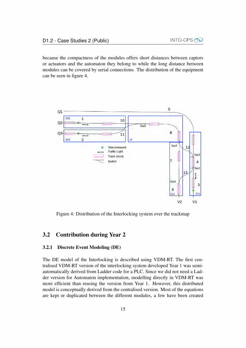
because the compactness of the modules offers short distances between captorsor actuators and the automaton they belong to while the long distance betweenmodules can be covered by serial connections. The distribution of the equipmentcan be seen in figure 4.
Figure 4: Distribution of the Interlocking system over the trackmap
3.2 Contribution during Year 2
3.2.1 Discrete Event Modeling (DE)
The DE model of the Interlocking is described using VDM-RT. The first cen-tralised VDM-RT version of the interlocking system developed Year 1 was semi-automatically derived from Ladder code for a PLC. Since we did not need a Lad-der version for Automaton implementation, modelling directly in VDM-RT wasmore efficient than reusing the version from Year 1. However, this distributedmodel is conceptually derived from the centralised version. Most of the equationsare kept or duplicated between the different modules, a few have been created
15

D1.2 - Case Studies 2 (Public)
specifically for the distribution. So while the safety kernel of the centralised in-terlocking model contained 180 equations, the distributed one has 250 equationsshared between the five modules (85 for ZV1, 49 for ZV2, 37 for ZQ2 and ZQ3and 39 for ZP). The distribution of the model introduced a new and important fea-ture to the system: message communication. The five interlocking modules needto communicate over long distance and with different signals. For this purpose wedesigned a ring network protocol and each module possesses a networking layerable to transmit and treat messages. This network function is also a part of theVDM-RT model and this gives benefits in the simulation.
Composition of a moduleEach of the modules contains inputs, local and output variables. Inputs come fromsensors (track circuits, states of relays, and states of switches), commands fromthe train and messages from other modules. Outputs are commands to relays (con-struction and destruction), commands to switches (left and right) and commandsto light signals. Locals have two purposes: to compute intermediate variables andto reflect the state of a distant module. Those variables form the system of booleanequations.
3.2.2 Continuous Time Modeling (CT)
The CT model from Y1 has been reused and modified for use with the new INTO-CPS Co-simulation Orchestration Engine (COE). It consists of a train in motionover a changing track-map. The train starts or stops at a signal light, and advanceson the track-map given the track chaining. The length of the track, the chaining oftrack and switches and the positions of the sensors and actuators are parametersof the CT mode. They are stored in text files and read during the execution ofthe simulation. The signal authorisation and the switche positions are granted bythe interlocking system. The maximum speed of the train at a certain positionis computed by the CT model, in accordance with the safe breaking methods.During Y2, we modified the model by better separating the parts: parameters,trains, Traffic Light Manager, RelayBox, MIC Manager and CommandPcc as canbe seen in figure 5.
The blocks help to simulate hardware parts of the interlocking. Mainly, RelayBoxand Mic Manager simulate the behaviour of the safety relays and the switches.They are triggered by the commands of the DE model and provides delayed con-trol variables for proofreading. CommandesPcc was a set of signals used for com-mand or parametrisation of the DE system. It was later removed and its contentswere changed into parameters.
16

D1.2 - Case Studies 2 (Public)
Figure 5: Highest block level of the CT model
Then the model was reshaped for modularity. A higher level of abstraction wasadded: figure 5 shows the simulation level which add the possibility to use differ-ent refinements and thus different simulations. SIL simulation can be run in twodifferent tools: Crescendo or the new INTO-CPS COE. This abstraction model isthe starting point of both kind of simulations. The Crescendo Interface block con-tains the arrays of variables for the Crescendo co-simulation and both TrainFMUand Relay Box can generate an FMU for COE co-simulation.
Figure 6: Architecture of SIL setting
For Hardware in the loop (HIL) co-simulation, we fused the blocks Crescendo -Interface and RelayBox into one abstract interface block. The interface model isbasically a wrapper that communicates with the hardware outside of the computer,which will be detailed in section 3.2.5. The interface between both boxes is thesame for SIL and HIL co-simulation: RemoteCommand and TrackCircuit fromtrain to Interlocking and Switch positions and Traffic light from Interlocking totrain.
17

D1.2 - Case Studies 2 (Public)
Figure 7: Architecture of HIL setting
Inside of the TrainFMU sub-model we added a way to manage a variable numberof trains. Inputs of the sub-model are distributed to the instances of trains andoutputs are computed from their outputs (boolean disjunctions or conjunctionsdepending on the signal).
2D InterfaceFor the purpose of demonstration, simulation graphs are not enough. We need tobetter represent the execution of the simulation. Therefore, we used the mecha-tronic module in 20sim to build an animated representation of the trains and theirdashboards. This work is planed for Y2 but still in progress.
3.2.3 FMU Generation
CT model: Trains: Generating an FMU for the 20sim CT model of trains wasnot straightforward. Unfortunately, three aspects of the model were not sup-ported at the moment of the test: tables, events by the 20sim FMU generatorand arrays by the COE. Arrays have been flattened to scalars, tables werereplaced by statical arrays put directly in the model. This lowered the pos-sibility of evolution of the model but does not change its meaning. Eventswere a larger problem: the calculation of most equations of the model werebased on events and it has not been possible to remove the concept of eventwithout breaking the model. Thus instead we build a lighter version of themodel. It modelled movement of the train and activation of the sensors butneither safe-breaking, derailment or slope management.
CT model: Relays: The FMU for Relays was generated without any problems.
DE model: VDM Interlocking: Generating an FMU from VDM required onlyto adapt the interface for scalars like the CT model and use the dedicatedFMI library.
18

D1.2 - Case Studies 2 (Public)
Figure 8: The TrainFMU Submodels
DE model: HIL wrapper: The HIL FMU wrapper is still in progress. The planis to generate the interface with 20sim or Modelio and manually write thecontent of the FMU (message packing and sending through the network).This will be done until the end of Year 2.
3.2.4 Co-simulation
Co-simulation using Crescendo was a great success during Year 1 and is still suc-cesfull with the models of Y2. Achieving the same goal using FMU faced someconstraints on models (see before) and exploitation of the results but was also asuccess.
Crescendo Co-simulationCrescendo was for us a reference for co-simulation, therefore the new CT andDE model needed to pass the test of Crescendo before going further in testing the
19

D1.2 - Case Studies 2 (Public)
Simulation Simulation Crescendo COEName duration duration durationQ3V2 init 15 24 18Q3V2 full 40 55 20Q3V1-V1Q3 70 92 40
Table 2: Duration of simulations
new INTO-CPS tool chain. The co-simulation was progressing well and withoutadjusting the model, mostly because those models were derived from a versionthat was already able to co-simulate in Crescendo. The most noticeable problemwas the speed of the simulation. The full simulation of a single train passing (40sec of simulated time) was taking 55 seconds on an average laptop (table 2).
Figure 9: Co-simulation of the route Q3-V2 with Crescendo
COE Co-simulationAfter correct generation of the FMUs, co-simulation with the INTO-CPS COEwas a very simple task. Setting the configuration and connecting the interfaces inthe application is very easy and there is very little room for user mistyping. Thesimulation is fast and gives immediate results. Graph results may not be as easyto read as in Crescendo but the raw Data can be read with external software.
FMU generation from 20sim and VDM and COE co-simulation is fast and reli-able. The process of generating a new FMU for a modified model is very fast soit’s possible to immediately test variants in co-simulation.
20

D1.2 - Case Studies 2 (Public)
3.2.5 Hardware In the Loop
Centralized VersionThe centralised version of the interlocking has lead to the realisation of a ded-icated Hardware in the Loop prototype. It consists of a micro-controller devel-opment board running the interlocking automaton software. On this board, weadded LEDs and relays to reproduce the real interlocking system running on site.This board has been connected to the simulator running on the PC and was usedto validate the accuracy of the simulation. The software running on the boardhas been translated by hand, being too early in the project for code generation.The co-simulation with centralised HIL was running only 20-sim on the PC: the20-sim safe-breaking CT model and a 20-sim wrapper. This validated the contin-uous CT model but lacked the use of the COE. This should be improved with thedistributed HIL prototype.
Figure 10: First Hardware in the Loop prototype
Distributed VersionThe second version of the HIL prototype was for the distributed Interlocking. Forthis prototype we needed six independent modules, one for Ethernet communi-cation with the simulator and five for the parts of the interlocking. We chooseto design dedicated boards for the integration of the micro-controllers and theirequipments. Each board is able to lock three relays for route reservation, manip-ulate two switches, three track circuits and one pair of signal lights. The centralmodule plays only the role of an interface, it sends and receives messages fromthe computer running the simulation and converts them to TTL signals (Transistor-Transistor Logic) for the Interlocking modules, simulating the actual sensors and
21

D1.2 - Case Studies 2 (Public)
actuators of the system.
The communication between the modules is handled by a ring network of RS-232connections. Each message is sent to the left neighbour and forwarded until itreaches its destination.
On each module, LEDs represent the state of the equipments, yellow for switches,blue for routes and red/green for the authorisation light.
This work still needs to be completed, the demonstration will be satisfying whenwe will be able to use the C code genereted from VDM-RT, embed it on the boardand run the distributed system along with the CT simulation on the PC.
Figure 11: The distributed Hardware in the Loop prototype
3.2.6 Improvement for Industrial Development
Year 2 was the occasion to produce a new product, the Distributed InterlockingSystem, comparable to the one produced during Year 1, the Centralized Interlock-ing System but with the tools provided by INTO-CPS. The main benefits fromusing the INTO-CPS tools are in the verification and validation phases of the V-cycle. The immediacy of the simulator tests reduces greatly the time betweensuccessive versions. Moreover, most of the testing can be executed at a higherlevel of abstraction using models which is sufficient for co-simulation. Of coursethe implementation of the model via code generation will also be submitted to aserie of tests later in the process, but the corrections during these tests will con-cern only implementation problems (scheduling, I/Os, . . . ) that could be found
22

D1.2 - Case Studies 2 (Public)
and solved with simple unitary tests.
3.3 Industrial needs and assessments
Table 3 presents an overview of ClearSy’s need for the INTO-CPS tool chain. Inthe following part, we detail each ClearSy’s (CLE) needs. Compared to Year 1,fulfilment of the needs by the INTO-CPS tools has been added to compare withthe baseline tools.
3.3.1 Cle 1: ClearSy time Modelling
• DescriptionThe tool must enable to express delays of system’s actions/steps. The toolmust enable the description of delay and the duration of physical compo-nents such as the commutation of relays and the state changes of the mo-torised switches. Also, it must be possible to set the time cycle of a microcontroller.
• Related Baseline Tools Requirements[LPO+16] Requirements 0003-0005 are related because the modeling oftime step could be done at the co-simulation level.
• Method of verificationWhile modeling the Railway signalling system using 20-Sim, the durationof state changes of the relays and switches were modelled using the 20-Sim operator “tdelay” (Indicators: succeed: yes/no, rate of success overcases). Cycle-time of interlocking software were also modelled using aClock operation that consumes a duration (using the VDM-RT operator ”du-ration”).
• Assessment: achievedIn all our case studies, modeling delays and cycles times were achieved inVDM-RT and 20-Sim. Indicator: 100%
3.3.2 Cle 2: ClearSy time Simulation
• DescriptionThe tool should simulate delays/cycle time of system’s actions/steps. Thetool should enable the description of computational delays and duration ofcommutation of relay in a signalling system.
23

D1.2 - Case Studies 2 (Public)
• Related Baseline Tools Requirements[LPO+16] Requirements 0003-0005 is related because the simulation oftime could be done at the co-simulation level. Requirement 0024 - is im-portant to be as precise as possible.
• Verification MethodClearSy attempted to simulate the Railway signalling system using 20-Simand VDM-RT. The switching of the relays should be simulated. Cycle-time should be simulated (Indicators: succeed: yes/no, rate of success overcases).
• Assessment: Partially achievedThe PLC time cycle and the delays of state changes for relays and mo-torised switches have been successfully simulated and also co-simulatedwith Crescendo. Thus, the tdelay operator from 20-sim is not imple-mented in FMU generation. The COE co-simulation required a modifica-tion of the model that removed this aspect. Indicator: 75%
3.3.3 Cle 3: ClearSy time Trigger Modelling
• DescriptionThe tools must contain, at least in one of their languages, a trigger artifactbased on time or delay.
• Related Baseline Tools Requirements[LPO+16] Requirements 0003-0005 is related because the simulation oftime could be done at the co-simulation level.
• Verification MethodVDM-RT was tested for the ability to code time based trigger.
• Assessment: achievedIt has been possible to set the duration of a computation unit using theVDM-RT CPU class. Cycle-time of interlocking software has also beenmodelled using a Clock operation that consumes a duration (using the VDM-RT operator ”duration”). The ”TON” and ”TOF” functions - from the LAD-DER code that enable to handle delay before triggering a signal or to hold asignal constant during a period of time- have been handled in VDM-RT bycomputing explicitly at each micro-step duration, the total elapsed time. INfunction of the elapsed time the TON/TOF operators decide the triggering.Indicator: 100%
24

D1.2 - Case Studies 2 (Public)
3.3.4 Cle 4: ClearSy time Trigger Simulation
• DescriptionThe tool should simulate the trigger based on time or delay. In order tobe able to synchronise with relays, and to express cycle time, it should bepossible to simulate in the software logic the clock or delay enabling topostpone the triggering of operations.
• Related Baseline Tools Requirements[LPO+16] Requirements 0003-0005 are related because the simulation oftime could be done at the co-simulation level. Requirement 0024 is impor-tant to be as precise as possible.
• Verification MethodVDM-RT will be tested for simulating the code of time based trigger. (In-dicators: succeed: yes/no, rate of yes over cases).
• Assessment: achievedIt has been possible to simulate the duration of a computation unit usingthe VDM-RT CPU class. Cycle-time of interlocking software has alsobeen simulated using a Clock operation that consumes a duration (using theVDM-RT operator ”duration”). The ”TON” and ”TOF” functions - fromthe LADDER code which enable to handle delay before triggering a signalor to hold a signal constant during a period of time- have been simulated.Indicator: 100%
3.3.5 Cle 5: ClearSy checking
• DescriptionThe tool should enable to check logical consistency at the level of co-simulation.
• Related Baseline Tools Requirements[LPO+16] Requirements 00032 to 00035 are Model-checking based re-quirements( discrete Model-checking, continuous Model-checking and global(co-simulation) Model-checking). Their achievements are important for Cle 5requirement industrial achievement.
• Verification MethodNon collision invariant or Overall delay should be checked. For instance theduration of switching of relays which was missing in ClearSy’s first proto-type and which caused an error at the testing phase on the industrial site,
25

D1.2 - Case Studies 2 (Public)
could be earlier found out with the help of the model checker.Indicator: succeed yes/no, rate of yes over casesThis should be done by model-checking by VDM-RT/RT-Tester/20-Sim. (Indicator: number logical of consistencies checked/ all logical consisten-cies)
• Assessment: not achievedAt Y2, global Model-checking has not been tried yet. It has been possibleto check invariant at the level of VDM-RT, and to inject error warning inthe 20-Sim model when continuous invariant is falsified (detection of de-railment). Indicator: 25%
3.3.6 Cle 6: ClearSy Simulation Scalability 1
• DescriptionThe tool could simulate real size Railway map evolution and trains move-ments.
• Related Baseline Tools Requirements[LPO+16] Requirement 0024, since it is important to control Simulator inorder to avoid side effects from computation latency.
• Verification MethodIndicator: Number of simulated tracks (and track circuits sensors), cross/joins(and join sensors) and related equations of simulation of train movement(20-Sim).
• Assessment: Partially achievedThe railway case study provided several csv files that store track map data(joins, traffic light, track circuit...) . Modeling the data for FMU generationis more complicated than for baseline tools. Data in csv files could not beread by the CT FMU. CT model has been adapted for FMU generation andcsv import has been removed. Indicator: 75%
3.3.7 Cle 7: ClearSy Simulation Scalability 2
• DescriptionThe tool could simulate real size railway signalling variable evolutions.
• Related Baseline Tools Requirements[LPO+16] Requirement 0024, since it is important to control Simulator inorder to avoid side effects from computation latency.
26

D1.2 - Case Studies 2 (Public)
• Verification MethodIndicator: number of signalling variables and logic that are simulated intoVDM-RT.
• Assessment: achievedDuring Y2, the number of variables of the VDM-RT model of interlockinghas increased due to the distribution. The simulation and co-simulation hasbeen successfully achieved. Indicator: 100%
3.3.8 Cle 8: ClearSy Simulation Exploration Scalability
• DescriptionThe tools should integrate several heterogenous models seamlessly.
• Related Baseline Tools Requirements[LPO+16] Requirements 0018-0020 could be necessary in order to assessthe maximal/minimal value from a range of parameters. The guidance re-quirements 0073, 0076 would be welcome.
• Verification MethodIndicators: possibility to assess the maximal/minimal/optimal value of aparameter from a range of test. Use case : rollback case maximal valueassessment, availability maximal value assessment, maximum duration as-sessment of train movement.
• Assessment: not achievedThe INTO-CPS tools now allow to sweep a range of parameters at the levelof co-simulation, only the train speed parameter has been tested so far. In-dicator: 25%
3.3.9 Cle 9: ClearSy Simulation Accuracy Confidence
• DescriptionThe tool could make clear the mechanisms, the accuracy and confidence ofthe simulation. It could be possible to handle and make clear the simulationof ordinary differential equations, with discontinue acceleration. It couldbe possible to model, explain and simulate multi-masses movement.
• Related Baseline Tools Requirements[LPO+16] Requirements 0045, 0047, 0055, 0058, 0061, 0065 : Seman-tics are necessary in order to keep accuracy and confidence. Quantifiable
27

D1.2 - Case Studies 2 (Public)
simulation tolerance at the INTO-CPS co simulation are necessary to keepaccuracy.
• Verification Method-20-Sim discontinuity handling (yes/no, accuracy/explanations)-20-Sim-Crescendo/COE maximal/minimal value assessment for a range oftest case at the co-simulation level, margin error (rollback, is there marginerror)
• Assessment: not achievedThe 20-Sim modeling successfully handles the discontinuity of the accel-eration because of the change of the track map (and so because the slopemay change), or because of an emergency braking. However, discontinuityis not supported for FMU generation. Indicator: 25%
3.3.10 Cle 10: ClearSy Seamless integration
• DescriptionThe tool should easily enable integrating several heterogeneous models.The co-modeling level should enable modeling a continuous train move-ment, model the track map (with discrete information), model the interlock-ing signalling software and model the electrical relays/switches.
• Related Baseline Tools RequirementsThe [LPO+16] guidance requirements 0067, 0071, 0076 are concerned.Help for modeling at the co-simulation level is concerned: Requirements0049 and 0050, 0051, 0052.
• Verification MethodThe Crescendo gluing/orchestration engine tool has been tested.FMI based co-simulation has been tested.Indicator: co-simulation: yes/no/partially achieved, rateduration to ”develop co-simulation”Is it FMI compliant ?
• Assessment: partially achieved
The FMI co-simulation of VDM-RT and 20-Sim has been successfully achievedbut with the use of a degraded CT model(see above part of co-simulation).Indicator: 75%
28

D1.2 - Case Studies 2 (Public)
3.3.11 Cle 11: ClearSy Distributed Modelling
• DescriptionThe tool should enable the modeling of distributed hardware, with commu-nication delay.
• Related Baseline Tools RequirementsIn [LPO+16] the requirement 0024, related to model communication delaysat the co-simulation level is concerned.
• Verification MethodThe co simulation with 20-Sim, VDM-RT and the COE has be assessedagainst the use case of distributed interlocking (distributed communicatingHardware)
• Assessment: achievedDuring Y2 a distributed model of Interlocking has been produced and usedfor co-simulation, using simulated communications. Indicator: 100%
3.3.12 Cle 12: ClearSy Code generation
• DescriptionThe tool should easily enable generating code (C) or binary (HEX) withcompatible facilities, complying with safety critical standards without toomuch need for manual patch.
• Related Baseline Tools Requirements[LPO+16] requirements 0037, 0042, 0044
• Verification MethodVDM-RT Interlocking software generation (for code execution) on Pic 32micro controllers for simulating interlocking.Indicator: achieved or not, duration to set the generation
• Assessment: not achievedAt M22 code generation is still in progress. Early prototypes have beentested and look promising. Indicator: 50%
3.3.13 Cle 13: ClearSy certification Safety
• DescriptionThe INTO-CPS tool chain should provide quality arguments for a possible
29

D1.2 - Case Studies 2 (Public)
certification kit (or any means to ease safety case) or redundant validationchain.- what is the global level of confidence ? what elements are available tobe used for safety case ? For each formalised modeling language (such asOpenModelica and VDM-RT) the language provider should also provideevidence that the corresponding simulator adhere to the formal semantic oftheir language.
• Related Baseline Tools RequirementsThe requirements 091 and 092 from [LPO+16] are critical for justificationof well-foundedness and safety handling. [LPO+16] Requirements 0045,0047, 0055, 0058, 0061, 0065 : Semantics are necessary in order to keepaccuracy and confidence. Quantifiable simulation tolerance at the INTO-CPS co simulation are necessary to keep accuracy.
• Verification MethodIndicator: Safety certification kit/method: yes/no
• Assessment: not achievedAt the first year, there is no available clear (formal) semantic of VDM-RT,20-Sim or OpenModelica and Crescendo. Moreover, there is no certifica-tion that the baseline tools behave as their specified semantic. Neither theco-simulation engine, or simulation engine, provide tolerance margin of theresulted simulations. There is no redundant validation chain for safety pur-pose. There is no certification kit. Indicator: 0%
3.3.14 Cle 14: CLearSy Failure Modelling
• DescriptionThe tool could enable modeling degraded mode at the co-simulation level.
• Related Baseline Tools Requirements[LPO+16] guidance requirement 0082 is critical. The interrupts mecha-nisms are also important at requirement 0056.
• Verification MethodVDM-RT/20-Sim. Model Emergency braking phase. Indicator: yes achieved/no/ partially
• Assessment: not achievedIt hat not yet been tested to model faulty behaviour in our CT model at theco-simulation level. Indicator: 0%
30

D1.2 - Case Studies 2 (Public)
3.3.15 Cle 15: ClearSy Traceability
• DescriptionThe tool should enable to coherently organise requirements and system-atically to warn the user about missing checking of requirements againstsimulation or automatic checking tools.
• Related Baseline Tools RequirementsFrom the deliverable [LPO+16], the requirements 0089 and 0090 are criticalfor traceability and impact analysis. [LPO+16] guidance requirement 0074is welcome. Requirements 0012-0017 are important.
• Verification MethodModelio testing of requirements handling (Indicator: duration to set a re-quirement),traceability (indicator : yes/no)easy checking (indicator duration to Set/launch checking)dealing with versions , indicator : yes /no
• Assessment: Partially achievedDuration to set a requirement w.r.t. internal ClearSy tools: writing a fewExcel requirements: 10 min, writing the same Modelio requirements: 12min.There is traceability facility, but not between a requirement and a piece ofcode (some area in the code), or a document (system, Hardware) and notdocumented in the INTO-CPS project yet.An easy checking is possible in theory but not documented in the INTO-CPS project yet.Indicator: (50%) .
3.3.16 Cle 16: ClearSy 3D animation
• DescriptionIn the baseline tool 20-Sim it is possible to have a 3D animation of theprogress while being simulated. It would be essential to keep this kind offunctionality in the multi-model FMI based co-simulation as well. A 3danimation would be useful for better co-simulation understanding, with anincreasing number of variables, it becomes difficult to follow the progres-sion of a simulation.
• Related Baseline Tools RequirementsFrom the deliverable [LPO+16], the requirements 0093 is critical.
31

D1.2 - Case Studies 2 (Public)
• Verification MethodExistence of such available 3D-animator using FMU
• Assessment: Partially achievedThe 3D animator embedded in 20-Sim has been made compatible with FMI.A model is being designed for the Railway Use-case but has not been testedin cosimulation yet.Indicator: (60%) .
32

D1.2 - Case Studies 2 (Public)
Tabl
e3:
Cle
arSy
’sN
eeds
Nee
ds.
Insi
ght
Prio
rity
Obj
ectiv
eY
1in
dic.
Y2
indi
c.D
iff.
Acc
ept.
Cle
1E
xpre
ssde
lays
MY
ear1
100%
100%
+0%
Ach
ieve
dC
le2
Sim
ulat
ede
lays
SY
ear1
100%
75%
-25%
Part
ially
achi
eved
Cle
3M
odel
trig
gert
ime
MY
ear1
100%
100%
+0%
Ach
ieve
dC
le4
Sim
ulat
etr
igge
rtim
eS
Yea
r110
0%10
0%+0
%A
chie
ved
Cle
5C
heck
ing
logi
calr
eqs.
SY
ear2
25%
25%
+0%
Not
Ach
ieve
dC
le6
Sim
ulat
etr
ack
map
CY
ear1
100%
75%
-25%
Part
ially
achi
eved
Cle
7Si
mul
ate
sign
allo
gic
CY
ear1
100%
100%
+0%
Ach
ieve
dC
le8
Eas
ySp
ace
expl
orat
ion
CY
ear2
0%25
%+2
5%N
otac
hiev
edC
le9
Ssim
ulat
orA
ccur
acy
CY
ear3
25%
25%
+0%
Not
Ach
ieve
dC
le10
Inte
grab
ility
ofM
odel
sS
Yea
r165
%75
%+1
0%Pa
rt.A
chie
ved
Cle
11D
istr
ibut
edSy
stem
sS
Yea
r10%
100%
+100
%A
chie
ved
Cle
12G
ener
ate
(Cor
Hex
)S
Yea
r325
%50
%+2
5%Pa
rtia
llyA
chie
ved
Cle
13C
ertifi
catio
nki
tS
Yea
r30%
0%+0
%N
otA
chie
ved
Cle
14D
egra
ded
mod
eC
Yea
r20%
0%+0
%N
otA
chie
ved
Cle
15O
rgan
ize
reqs
.S
Yea
r250
%50
%+0
%Pa
rt.a
chie
ved
Cle
163D
Vis
ualis
atio
nS
Yea
r150
%60
%+1
0%Pa
rt.a
chie
ved
33
D1.2 - Case Studies 2 (Public)
4 Agriculture Case Study
This is the public version of the agricultural case study which provides a generaloverview. A more detailed version of the same document can be found in theconfidential version.
4.1 Introduction
This case study is provided by the Danish company Agro Intelligence (AI) and itis focused on the evaluation and development of an agricultural robotic platform.This document also builds on the work submitted in the D1.1c deliverable afterthe first year of the INTO-CPS project [EGH15].
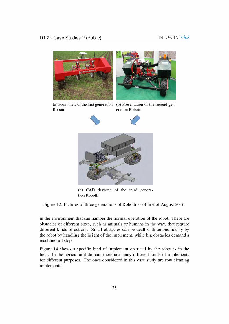
Figure 12 illustrates the three different generations of the robot over time, until thewriting of this deliverable. The work presented in this deliverable will primarilybe focused on the current version under development and secondly provides anupdate on the modelling of version 2 of the robot. The reason why the mainfocus is on the new version of the robotic platform is to evaluate how the INTO-CPS tool chain can be used to support rapid development of such an agriculturalsystem.
4.2 Agriculture case study
This case study is focused on the agricultural robotic platform Robotti. An earlyversion of this robot can be seen in Figure 12a. Robotti is designed as a low cost,semi-autonomous machine to apply different kinds of soil and crop treatmentsthrough agricultural tools called implements. Examples of implements could besowing, weeding, spraying or row cleaning tools.
4.2.1 Description
The robot was initially conceived to be deployed and operated in fields structuredin rows. An overview of the working environment is shown in Figure 13. Thisfigure shows the start position where the robot is normally deployed and it repre-sents with arrows the trajectory it follows. The robot transits from one row to theadjacent one in the turning areas. The field in which the robot is deployed is notnecessarily flat and it could present different kinds of slope changes. In additionto the plants and the soil that have to be treated, there are other external elements
34
D1.2 - Case Studies 2 (Public)
(a) Front view of the first generationRobotti.
(b) Presentation of the second gen-eration Robotti
(c) CAD drawing of the third genera-tion Robotti
Figure 12: Pictures of three generations of Robotti as of first of August 2016.
in the environment that can hamper the normal operation of the robot. These areobstacles of different sizes, such as animals or humans in the way, that requiredifferent kinds of actions. Small obstacles can be dealt with autonomously bythe robot by handling the height of the implement, while big obstacles demand amachine full stop.
Figure 14 shows a specific kind of implement operated by the robot is in thefield. In the agricultural domain there are many different kinds of implementsfor different purposes. The ones considered in this case study are row cleaningimplements.
35

D1.2 - Case Studies 2 (Public)
Figure 13: Example of a field where Robotti could be deployed.
Figure 14: Two different row cleaning implements mounted on Robotti and tillingthe soil.
36

D1.2 - Case Studies 2 (Public)
4.2.2 Requirement and Specification
The industrial project Robotti is composed of a number of requirements and sce-narios. In order to present an approachable case for the INTO-CPS researchproject a subset of eight functional requirements has been formulated as Use Cases(UC). An overview of these use cases is provided in Figure 15.
The overall use case is R1 and it is decomposed into additional seven use cases.
Figure 15: SysML use case diagram giving an overview of the services the robotcontroller has to provide.
The requirements specified in this section are related to robot navigation and im-plements safety control. Most of the requirements presented in Agro Intelligence(AI) are functional requirements and are specified as UC. More detailed descrip-tions of the use cases are provided in the sub-sections below.
Requirement 1: UC Control Robotti (Top Level UC)
• Description: The user should be able to control Robotti so it is possibleto work the crop-fields. This is a top level use case that is refined in moreconcrete services offered by the system in the following UC descriptions.
37

D1.2 - Case Studies 2 (Public)
• Method of Verification: Model simulation and system testing.
Requirement 2: UC Operate Manually (Free Drive)
• Description: The human operator should be able to operate manually Robottiin the crop-fields, being able to steer it and control its speed. The manualmode is denoted as Free Drive, since it allows the human operator to controlthe robot externally.
• Method of Verification: Model simulation and HiL system testing.
Requirement 3: UC Operate Automatically
• Description: Robotti should be able to navigate a field independently with-out requiring the constant input of a user.
• Method of Verification: Model simulation and system testing.
Requirement 4: UC Control Implement
• Description: It should be possible to activate the implement and controlits height if needed. When Robotti operates automatically the implementheight can be changed depending on the robot’s position in the field.
• Method of Verification: Model simulation and system testing.
Requirement 5: UC Drive Row
• Description: Robotti should drive along the crop-rows of the field in whichit is deployed and stay within them.
• Method of Verification: The model of the robot will be simulated takingthe effect of disturbances and irregularities of the crop and soil into consid-eration.
Requirement 6: UC Move to Next Row
• Description: Robotti should be able to transit between rows through a turn-ing area. Implements should be lifted/deactivated before starting the turnand lowered/activated when the turn is completed. Dependent on the imple-ment, the robot might need to be paused in its steering and driving, until theoperation is completed.
38

D1.2 - Case Studies 2 (Public)
• Method of Verification: The model of the robot will be simulated havingthe robot deployed close to the end of a row.
Requirement 7: UC Handle Obstacle
• Description: Robotti should be able to detect obstacles in the row in whichit is operating. Examples of obstacles can be a bird nest, a person or a deer.
• Method of Verification: The model of the robot will be simulated in dif-ferent scenarios with obstacles of different sizes placed in different parts ofthe field.
Requirement 8: UC Emergency Stop
• Description: Robotti should be able to perform an emergency stop andexecute a predictable stop behaviour. Supply to the motor (current/diesel)will be cut via hardware and a human operator notified. The controllers willstop their current operation and move back to idle mode.
• Method of Verification: The model will be simulated through differentsafety/critical scenarios.
Requirement 9: NF Platform usage
• Description: The solution modelled and considered in this case study shouldtarget the controller platforms intended to be used on Robotti. These areLinux platform running with the Robot Operating System (ROS) [QCG+09]and B&R Programmable Logic Controllers (PLC)1.
• Method of Verification: Does not apply.
4.3 Modelling
This section describes the modelling that has been done using the INTO-CPS toolsduring this second year of the project. The modelling tools that have been used forthis chapter are, Overture, 20-sim, OpenModelica and Gazebo/ROS. The main fo-cus is the third generation of the Robotti vehicle platform and the different aspect
1B&R is a company producing industrial automation controllershttp://www.br-automation.com/en/
39

D1.2 - Case Studies 2 (Public)
of the on-board sensors and actuators. The reason why Agro Intelligence has cho-sen to extend the chain with Gazebo/ROS [QCG+09] is explained below.
4.3.1 Gazebo and ROS
Simulation and 3D-visualisation make it possible to rapidly test algorithms, de-sign robots, and perform experimentation and testing using realistically modelledscenarios. Figure 16 illustrates one of the first versions of the next generation ofRobotti before the CAD models were made.
Figure 16: Visualisation of the upcoming third generation of the Robotti platformin Gazebo.
Gazebo offers the ability to accurately and efficiently simulate and visualise robotsin indoor and outdoor environments. In this case study, we mainly use Gazebo forvisualisation of the simulation result from COE, made with the models from 20-sim, Overture and OpenModelica. This kind of Gazebo visualisation of approachallows our development team to get early feedback from end users with a lesserunderstanding of all the utilised CPS technologies. Feedback from end users likean onion or cabbage farmer can provide valuable product feedback early in thedevelopment process, to ensure the development meets their demands.
Gazebo is mainly used for visualisation as stated in the description above, withthe exception of visual sensing and the field environment. Visual sensing can be a
40

D1.2 - Case Studies 2 (Public)
camera or a laser-range scanner sensor, which is intended to be used on Robotti.To model a camera system, it needs an actual input of a crop field and obstaclesto provide the correct output. By using the already created visualisation fromGazebo, a simulated image can be generated. To connect the INTO-CPS toolswith Gazebo, ROS is used to delegate communication back and forth.
In some of AI’s other research projects, the Gazebo/ROS combination is also be-ing used by the academic and industrial partners. We have chosen to also followthis path in this case-study, to allow for better inter-collaboration with the otherprojects.
Creating crop-fields for Robotti The different field scenarios Robotti must op-erate in is an important part of the case study. The crop type and field structurehave a significant impact on how Robotti should perform its task in the field. InFigure 17, examples are found of such crop-fields generated for Robotti to operatein. The simulated fields allow us to evaluate the results from the simulations, andare used as input for the visual sensor as objects in the environment.
(a) Cabbage Field (b) Corn Field
(c) Apple Orchard (d) Onion Field
Figure 17: Generated crop field examples
41

D1.2 - Case Studies 2 (Public)
4.3.2 Robotti Third Generation
The third generation of the robotti platform comes in two different versions, aversion with four-wheel steering and one with two-wheel steering as illustratedin Figure 18. Regarding industrial production, the first version currently intendedto be put into production is the two-wheel steered version. In both versions eachsteered wheel can be operated individually to provide a high degree of freedom indriving.
Figure 18: Planned steering freedom in the third generation of Robotti.
The two-wheel steered version is designed to be similar to a tractor and is intendedto provide similar functionality with and without a human operator driving therobot. The main difference is that the implement (examples could be cultivator orsprayer) will be mounted inside the frame and not behind.
A vehicle CT model 4.3.2 4.3.2 have been made for the third generation of Robotti.The main reason for the different models is to account for the two types of robotsand the progress of exporting capabilities from 20-sim this year. To export themore complex vehicle models, it requires variable step-size solver for FMU towork.
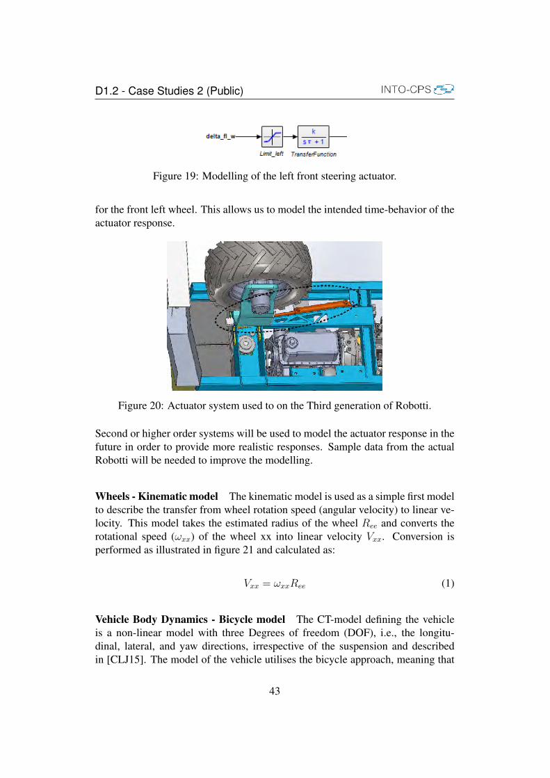
Actuators To steer the wheels on Robotti a hydraulic actuator is used for eachwheel as illustrated in Figure 20. The actuator drives the wheel using a rack andpinion gearing system that translates linear motion into rotation.
This steering system has been modelled as a first order transfer function in 20-sim.The limiting block ensures that the response is within the boundaries of the actualactuator. Each wheel is steered individually with a setup as illustrated in figure 19
42
D1.2 - Case Studies 2 (Public)
Figure 19: Modelling of the left front steering actuator.
for the front left wheel. This allows us to model the intended time-behavior of theactuator response.
Figure 20: Actuator system used to on the Third generation of Robotti.
Second or higher order systems will be used to model the actuator response in thefuture in order to provide more realistic responses. Sample data from the actualRobotti will be needed to improve the modelling.
Wheels - Kinematic model The kinematic model is used as a simple first modelto describe the transfer from wheel rotation speed (angular velocity) to linear ve-locity. This model takes the estimated radius of the wheel Ree and converts therotational speed (ωxx) of the wheel xx into linear velocity Vxx. Conversion isperformed as illustrated in figure 21 and calculated as:
Vxx = ωxxRee (1)
Vehicle Body Dynamics - Bicycle model The CT-model defining the vehicleis a non-linear model with three Degrees of freedom (DOF), i.e., the longitu-dinal, lateral, and yaw directions, irrespective of the suspension and describedin [CLJ15]. The model of the vehicle utilises the bicycle approach, meaning that
43

D1.2 - Case Studies 2 (Public)
Figure 21: Concepts in the kinematic tyre model
the lateral forces on the left and right wheels are assumed to be equal and summedtogether. This assumption holds for typical agricultural vehicle operation veloci-ties (<7.5 m/s) [KS10]. The bicycle structure is also known as a half-vehicle (Fig-ure 22). The model allows for yaw and lateral motion through adjustment of thefront wheel angle δf .
Figure 22: Dynamic bicycle model of the body of the Third Generation of Robotti.
The velocities u, v are at the Center of gravity (CG) of the vehicle. L is thewheelbase, where a is the longitudinal distance to the front wheel, and b is thelongitudinal distance to the rear wheel. For a constant forward velocity, the vehiclemotion is given by
m(v + uψ) = Ff,ycos(δf ) + Fr,y (2)
44

D1.2 - Case Studies 2 (Public)
where r is the angular rate about the yaw axis. Similarly, the vehicle yaw motionis expressed by
Izzψ = aFf,y − bFr,y (3)
where Izz is the moment of inertia along the yaw axis.
Implements In agriculture, implements are the tools that are mounted onto atractor, e.g. a cultivator or a sprayer. On the current version of Robotti the im-plement is attached to the vehicle by a three-point linkage, which is the standardway utilised by tractors. How this three-point linkage operates differ from vehi-cle to vehicle, but the general mechanical design is the same. A first three-pointlinkage model was created, as illustrated in Figure 23a, to mount different typesof implements.
(a) Cultivator modelling - first attempt (b) Sprayer modelling - first attempt
Figure 23: First attempts in adding implements to the Robotti tool career.
A revision of this first CT-model of the connector will be needed when the finalversion of Robotti has been made. In this second year of INTO-CPS, a sprayersystem has been the main focus of Robotti’s implements, illustrated in Figure 23b,since it can be used for multiple applications. In its current version, the model ofthe sprayer assumes all nozzles are driven using the same valve. In later versions,the intention is to make a model where each nozzle can be activated individually,in order to allow spot spraying.
4.4 Robotti Second Generation
The movement of the robot has been studied from the CT side by creating a kine-matics model of the vehicle. The 20-sim representation of the system is shownin Figure 24. This model takes the radius of the wheels Ree and the separationbetween them Tc into consideration, to describe the robot movement. Based on
45

D1.2 - Case Studies 2 (Public)
these parameters and on the distances travelled by the wheels, it is possible todetermine how the robot moves and what orientation it has.
Figure 24: 20-sim model of the Robotti second generation.
The model is symmetric since the construction of the robot is as well, meaningthat the mechanics of the left side of the robot are identical to the ones used on theright side.
The robot movement is described through a number of equations. The speed ofthe robot Vc is considered from the center of the robot, and described in terms ofthe rotational speeds of the right (ωr) and left wheels (ωl), as shown in equation 4and based on 4.3.2.
Vc =(ωrReee + ωlRlee)
2(4)
Considering the separation between the wheels Tc, it is also possible to determinethe yaw rate of the robot (ψ), as shown in equation 5. ψ is an angle defined withrespect to the XY frame. X and Y are defined with respect to the field.
ψ =(ωr − ωl)
Tc(5)
46

D1.2 - Case Studies 2 (Public)
Finally, based on these calculations it is possible to determine the location of arobot using the equation 6 for the X and Y coordinate axes respectively.
[xy
]= Vc
[cos(ψ)sin(ψ)
](6)
4.4.1 Sensors
Camera row-tracking For the camera sensor, we have two model versions forthe crop-row detection, one for using Gazebo and a simpler version using 20-sim.
(a) Basler camera intended to be used forrow-tracking on Robotti.
(b) Output from the tracking algorithmwith the Gazebo image.
Figure 25: Camera and simulated output.
The detection of the crop-row is done to ensure that Robotti can move safely in thefield without harming the individual plants. The Gazebo version utilises a cameraimage for the crop-row tracking algorithm, which provides an offset and an angleof the rows, as it is illustrated in Figure 25. The 20-sim version provides an outputsimilar to the tracking algorithm, but without the use of an image, as it is based ona map aware of the current robot and crop positions. The intention behind the 20-sim version is to imitate what the actual tracking algorithm would provide, andallow it to run with configurations that are not possible with the algorithm. Anexample of these configuration parameters could be higher real-time update rates,or improved or degraded detection results.
47
D1.2 - Case Studies 2 (Public)
4.4.2 Encoders
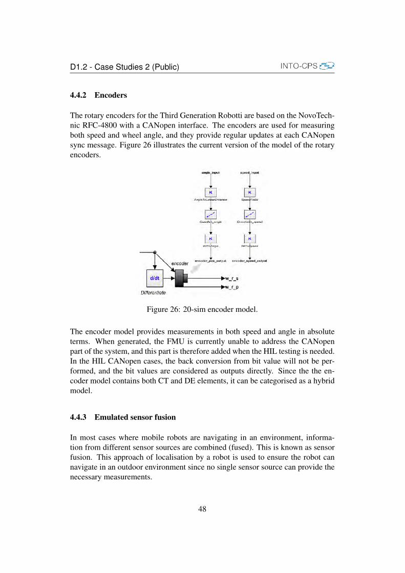
The rotary encoders for the Third Generation Robotti are based on the NovoTech-nic RFC-4800 with a CANopen interface. The encoders are used for measuringboth speed and wheel angle, and they provide regular updates at each CANopensync message. Figure 26 illustrates the current version of the model of the rotaryencoders.
Figure 26: 20-sim encoder model.
The encoder model provides measurements in both speed and angle in absoluteterms. When generated, the FMU is currently unable to address the CANopenpart of the system, and this part is therefore added when the HIL testing is needed.In the HIL CANopen cases, the back conversion from bit value will not be per-formed, and the bit values are considered as outputs directly. Since the the en-coder model contains both CT and DE elements, it can be categorised as a hybridmodel.
4.4.3 Emulated sensor fusion
In most cases where mobile robots are navigating in an environment, informa-tion from different sensor sources are combined (fused). This is known as sensorfusion. This approach of localisation by a robot is used to ensure the robot cannavigate in an outdoor environment since no single sensor source can provide thenecessary measurements.
48
D1.2 - Case Studies 2 (Public)
Making a complete sensor-fusion setup can seem a bit extreme in a modellingcontext, when it is wanted, for example, to test a navigation algorithm. To simplifythe process, a model has been made that emulates the expected behaviour of sensorfusion algorithm using 20-sim. The model can currently be in three differentstates:
1. Provides no data about the robot’s localisation
2. Provides current position but not the direction of the robot
3. Provides current position and the direction of the robot (pose)
For both case 2 and 3, the localisation data comes with an uncertainty estimate.
4.4.4 Controllers
The controllers documented here are designed for the third generation of Robotti,but should in theory also be applicable to the second generation of Robotti, withsome minor modifications.
4.4.5 High-level control structure
The state diagram in Figure 27 is used to represent how the robot reacts to dif-ferent external events, toggling between different operational modes. The manualmode is used for the operational setup, like mounting the implement, testing actu-ator functionality and driving the robot by wire. For high-level control, the robotalways starts in idle mode with all actuators in passive, but all sensors are bootedup. Currently, it is only possible to switch to FreeDrive directly, since to robotneeds a heading in order to go into AutomaticOperation. The heading determineswhich way the robot is turned globally, and is used to guide the robot correctlyinto the field, since both position and heading need to be known. The EmergencyStop occurs when a bumper action, safety button press or an unhandled situationoccurs.
4.5 Industrial needs and assessment
The industrial needs have been updated to match the current needs of Agro In-telligence. The description has been focused, and no new industrial needs havebeen added. An overview of AI industrial needs after year two is presented inTable 4.
49

D1.2 - Case Studies 2 (Public)
Tabl
e4:
Sum
mar
yof
Agr
oIn
telli
genc
ein
dust
rial
need
s.
Req
.C
ateg
ory
Sub
Cat
.D
escr
iptio
nPr
iori
tySt
atus
Ver.
AI
1Fu
nctio
nal
Tool
sC
++co
dege
nera
tion
MPa
rtia
llyac
hiev
ed2.
1fr
omV
DM
-RT
AI
2Fu
nctio
nal
Tool
sC
-cod
ege
nera
tion
MPa
rtia
llyac
hiev
ed2.
0fr
om20
-sim
AI
3Fu
nctio
nal
Tool
sH
iLan
dSi
LM
Part
ially
achi
eved
2.1
sim
ulat
ion
AI
8N
on-F
unct
iona
lPr
oces
sD
evel
opm
ent
SPa
rtia
llyac
hiev
ed2.
1M
etho
dolo
gyA
I9
Func
tiona
lTo
ols
Mod
elsn
apsh
otC
Ach
ieve
d2.
1an
dve
rsio
nco
ntro
lA
I10
Func
tiona
lTo
ols
Sim
ulat
ion
resu
ltssn
apsh
otC
Part
ially
achi
eved
2.1
and
vers
ion
cont
rol
AI
11Fu
nctio
nal
Tool
sG
azeb
oin
tegr
atio
nS
Part
ially
achi
eved
2.1
AI
12Fu
nctio
nal
Tool
s3D
anim
atio
nS
Part
ially
achi
eved
2.1
and
visu
alis
atio
n
50

D1.2 - Case Studies 2 (Public)
Figure 27: Overal Control statemachine structure in SysML form
The following sections provide a description of the industrial needs for the agri-cultural case study. These industrial needs are formulated as requirements.
4.5.1 AI 1: Code generation from VDM-RT
• Description: The tool must facilitate code generation from VDM-RT mod-els to C++. The target platform for this is embedded Linux and it must runeither as a standalone executable or within a ROS node.
• Method of Verification: Code generation from models of different controllogic of varying complexity. Testing of the generated code in a controlledsetup and comparison with expected results based on models. Measure-ment: percentage of VDM-RT modules translated; suitability as controlsoftware.
• Assessment: Partially achieved
51

D1.2 - Case Studies 2 (Public)
The code generation support from VDM-RT is close to fully developed forC-code, according to the baseline tool requirements. However, due to pri-oritisation of the developers of the VDM code generator to support C-codegeneration in the first place, its functionality is not fully suitable for AgroIntelligence since we need code generation to C++, and C++ code cannotrun in C-code environment. As AI has a different development time sched-ule than in the INTO-CPS requirements, i.e. before the code generator wasrequired to be ready, we had to code in both C++ and VDM manually. AIhas provided an example VDM-RT project for our target platform (embed-ded Linux with ROS) that can be used as a first step to validate when a C++code generator is ready for testing.
• Related baseline tools requirements: 0038
• Degree of achievement: 75%
4.5.2 AI 2: Code generation from 20-sim
• Description: The tool must facilitate code generation from 20-sim to C/C++software. The target platform for this is embedded Linux, and it must runeither as a standalone executable or within a ROS node.
• Method of Verification: Code generation from models of different controllogic of varying complexity. Testing of the generated code in a controlledsetup and comparison with expected results based on models. Measure-ment: percentage of 20-sim moduls translated; suitability as plant and con-trol software.
• Assessment: Partially achieved.20-sim models can be exported into C-code and FMU units for fixed step-size ODE solvers (Euler, Runge-Kutta 2, Runge-Kutta 4), that can be exe-cuted on Windows- and Linux-based computer units. The variable step-sizesolve has been implemented to allow the C-code generation to match theresponse in 20-sim. The Backward differentiation formula (BDF) solver iscurrently the only tool able to support some of the more vehicle models.This functionality is still needed to be implemented for code generation.
• Related baseline tools requirements: 0038, 0039, 0040
• Degree of achievement: 65%
52

D1.2 - Case Studies 2 (Public)
4.5.3 AI 3: HiL and SiL simulation
• Description: The tool must facilitate Hardware-in-the-Loop and Software-in-the-Loop simulation of 20-Sim and VDM models.
• Method of Verification: Co-execution of different models of increasingcomplexity with Hardware and Software realisations. Measurement: Yes/Nofor HiL and SiL; Percentage of simulated cases (from total of “pure” modelsimulations).
• Assessment: Partially achieved.At the writing of this chapter, only 20-sim and OpenModelica can provideexport of code that can be used for HiL and SiL testing. HiL is done via theFMUs and implemented manually on the particular Operating system andcontroller.
• Related baseline tools requirements: 0042, 0043, 0084, 0086, 0087, 0088
• Degree of achievement: 30%
4.5.4 AI 8: Methodology for the development of embedded real-time sys-tems.
• Description: The project must provide methodological guidelines to applya model-based engineering approach using the tools from INTO-CPS to thedevelopment of embedded real-time systems that constitute Cyber-PhysicalSystems.
• Method of Verification: Provided/Not provided. Applicability assessed byusing the tools in the case study. Measurement: Weighed percentage ofactivities not applicable and activities missing in proposed methodology.
• Assessment: Partially achieved.
The methodological guidelines for the development of embedded real-timesystems are in general terms achieved, but are lacking some specific exam-ples, which are relevant for mobile robots, such as the Robotti case study.We think these should be included in requirement 0084 with deadline inY3. It has been challenging to adapt them to our setup on Linux/ROS plat-form, and specific guidelines for mobile robots and their interaction withthe environment. For example, we would have liked to have more spe-cific guidelines for data exchange for GIS, and for sensor data transmission
53

D1.2 - Case Studies 2 (Public)
of GNSS, Camera, IMU or Laser-range scanner, which are important for aCPS technology like a mobile robot. A different development time schedulebetween AI and the INTO-CPS requirements, caused the mismatch betweenour needs and the available guidelines.
• Related baseline tools requirements: 0070 - 0076, 0084
• Degree of achievement: 60%
4.5.5 AI 9: Model snapshot and version control
• Description: The tool-chain should provide a way to keep track of the dif-ferent versions of the models that compose a co-model.
• Method of Verification: Provided/Not provided. Applicability assessed byusing the tools in the case study. Measurement: Yes/No. Degree of supportin multi-simulation setup.
• Assessment: Achieved.The way the INTO-CPS COE operates allows the FMU models to be dis-tributed in sub-folders, that allow for tools like git and svn the ability toversion control multi-models for the case studies. The same goes for themodels made within the tools 20-sim, Overture and OpenModelica. A chal-lenge still is to do version control directly on 20-sim *.emx files, since theycan represent visual blocks.
• Related baseline tools requirements: none.
• Degree of achievement: 99%
4.5.6 AI 10: Simulation results snapshot and version control
• Description: The tool should provide a way to keep track of the differentsimulation results of a co-model. This could enable that at any point of timea certain set of simulation results can be linked to a concrete version of themodels as well as the parameters used for the simulation.
• Method of Verification: Provided/Not provided. Applicability assessed byusing the tools in the case study. Measurement: Yes/No. Degree of supportin multi-simulation setup.
• Assessment: Partially achieved.When a simulation is executed via the COE, the exchange variables are
54

D1.2 - Case Studies 2 (Public)
stored in a time-stamp log file. A challenge that is still present is the abilityto match git/svn version with the simulation result.
• Related baseline tools requirements: none.
• Degree of achievement: 50%
4.5.7 AI 11: Gazebo integration
• Description: The project could enable the co-simulation of high-level con-trol models with Robot models running in the Gazebo environment.
• Method of Verification: Co-simulation of models of different complexity.Reading of sensors and control of actuators that are deployed in Gazebo. In-teraction with the Gazebo simulated world. Measurement: Yes/No. Degreeof support in simulation/multi-simulation setup.
• Assessment: Partially achieved.It is possible to interface with Gazebo using the interface Agro Intelligencehas made 4.3.1. A direct Gazebo FMU interface to the COE is still missingfor full completion.
• Related baseline tools requirements: 0001 - 0006
• Degree of achievement: 50%
4.5.8 AI 12: 3D animation/visualisation
• Description: The project should enable the visualisation of Robotti models.This will help to understand complex behaviour expressed in the model andfacilitate communication in multi-disciplinary engineering teams.
• Method of Verification: Provided/Not provided. Visualisation of co-simulationmodels. Ease of use. Quality of visualisation. Measurement: Yes/No.Weighed: Degree of support in simulation/multi-simulation setup; Time tocreate visualisation compared to “conventional” tool; Acceptance by engi-neers.
• Assessment: Partially achieved.
• Related baseline tools requirements: 0093
• Degree of achievement: 75%
55

D1.2 - Case Studies 2 (Public)
5 Building Case Study
In this section we provide the public version of the building case which providesa generic overview of the Year 2 case study of an HVAC Cyber-Physical System.A more detailed description can be found in the confidential version.
5.1 Introduction
The Year 2 case study contains a description of the public the building scenariodeveloped by UTRC, the design of the HVAC infrastructure the modeling ofthe involved Cyber-physical components and the results generated after the co-simulation using the INTO-CPS platform. The HVAC scenarios studied, will in-clude a Cyber-physical system surrounding a building area of a floor, consistingof two rooms and one zone composed by two areas. Each room temperature willbe controller by a Fan Coil Unit (FCU). The zone temperature will be controlledby two collaborated FCUs, each one for one of the two areas of the zone. TheFCU will consist of several vital elements that will control the fresh air temper-ature provided by the Air Handling Unit (AHU) to the room using air dumper,fan, coil and valves. The water that will heat or cool the air will be pressurizedand provided to each FCU by the Heat Pump Unit (HPU), currently not includedin the CT model. The described scenario will be modeled using the INTO-CPSbaseline tools as well as state-of-the-practice commercial tools and evaluated en-tirely in the INTO-CPS platform. After descriptions of SysML modeling, CT andDE models developed, we discuss the co-simulation results taken from the currentversion of the INTO-CPS engine for a series of controller scenarios. Finally weconclude with FMI co-simulation experiences and next steps towards year 3 usecase.
5.2 Building Case Study
The building case study will focus on modeling and analysis of energy and com-fort systems that control the temperature of connected rooms or areas inside abuilding premise as shown in figure 28. This Year 2 case study models encapsu-late several modules including a) Physical rooms and air flow modeling, b) FanCoil Units, c) Supervision of the FCUs d) Communication interfaces betweenmaster-slave FCUs, e) Communication between FCUs and Supervisor, f) Air-pipeconnections between FCUs and AHU, g) Water-pipe connections between FCUsand HPU, h) Air-Handling Unit controller and i) Heat Pump Unit load. Results
56

D1.2 - Case Studies 2 (Public)
have been generated from the newly developed Continuous and Discrete modelsfor Year 2 that are based on commercial HVAC products and control require-ments.
The current control strategy will compose a multi-model that will regulate FCUoperation, Supervision of FCUs, AHU operation and overall HVAC functionality.User inputs will be taken into account from rooms or zone thermostats and willcompared with current Room Air Temperature (RAT) sensed by the FCUs, trig-gering certain actions to the FCU(s). The FCU(s) having a direct connection witha supervisor device, will take a series of actions to reach the desired temperatureby a) regulating the air flow using its fan and the air-dumper, b) power up thecoil to heat the air if necessary, c) regulate the water pipe valves to control thecooled or heated air originated by the AHU, d) regulate the water pressure insidethe water pipes originated by the HPU, e) synchronize with the supervisor to co-ordinate with the rest of the FCUs and respectively -if needed- with the AHU andthe HPU.
Figure 28: Rooms and Zone level schematic for the Year 2 building case study
The main objective for the Year 2 case study is to respect high level requirementsthat span from temperature control of rooms and the zone , energy consumptionand safe operation of all of the devices that are involved in the HVAC system.One of the main reasons why the aforementioned fact remains a challenge, is theproduct line engineering approach currently followed by building automation in-dustries. In the current work-flow, different types of engineers contributing tothe creation of the same device are involved and affecting respectively the systemdesign. Verification of the generated models or code is enabled in stages of theproduct life-cycle that leave the system open to delays due to late error discov-ery. To this end, INTO-CPS and co-simulation solutions will not only bridge theidentified gap between engineers but also, enable verification of the output mod-
57
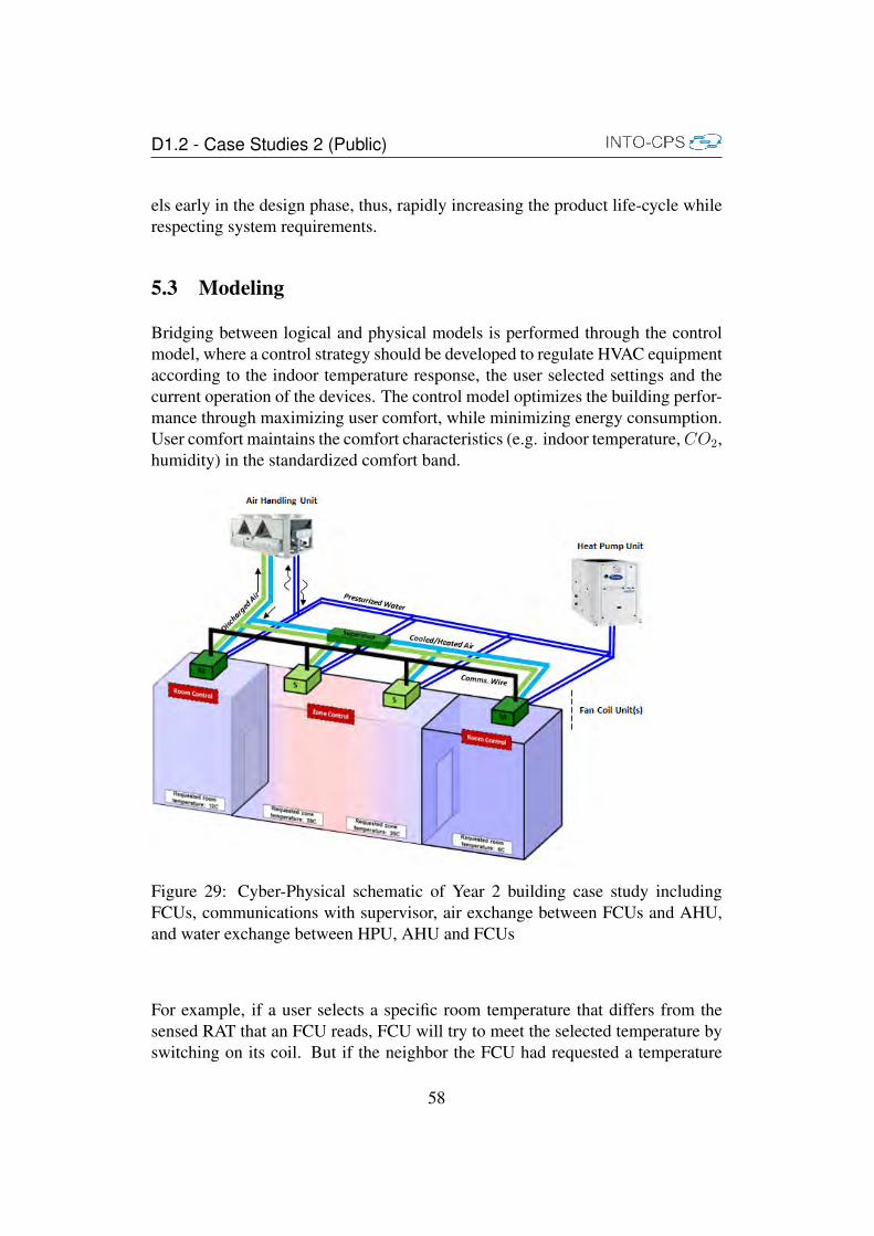
D1.2 - Case Studies 2 (Public)
els early in the design phase, thus, rapidly increasing the product life-cycle whilerespecting system requirements.
5.3 Modeling
Bridging between logical and physical models is performed through the controlmodel, where a control strategy should be developed to regulate HVAC equipmentaccording to the indoor temperature response, the user selected settings and thecurrent operation of the devices. The control model optimizes the building perfor-mance through maximizing user comfort, while minimizing energy consumption.User comfort maintains the comfort characteristics (e.g. indoor temperature,CO2,humidity) in the standardized comfort band.
Figure 29: Cyber-Physical schematic of Year 2 building case study includingFCUs, communications with supervisor, air exchange between FCUs and AHU,and water exchange between HPU, AHU and FCUs
For example, if a user selects a specific room temperature that differs from thesensed RAT that an FCU reads, FCU will try to meet the selected temperature byswitching on its coil. But if the neighbor the FCU had requested a temperature
58

D1.2 - Case Studies 2 (Public)
point that required additional water pressure from the Heat Pump Unit to heat theair, then the initial FCU could avoid switching the coil on as it can regulate watervalves to allow more (already heated) water to be driven inside it while closingvalves in the second FCU through the supervisor. Such a decision will increaseenergy savings, as the the coil will not be switched on and the Heat Pump will notrequire to be activated through a water rerouting solution.
Design Modeling
In this section initial requirements are described according to core functionalitydescribed for the FCUs unit, the supervisor and communication network, the AHUunit and the system as a whole. At the current level of the building use case, wefocus on the assessment of a subset of those requirements, as our main interest forthe Year 2 is to evaluate INTO-CPS platform usage.
The SysML design model defines the architecture of the CPS at a high level.From this high level description, we derive the specifications for the FMUs thatcompose the multi-model of the system and the connections between them. TheFMU specifications are satisfied by the constituent models elaborated using theOverture VDM and Dymola Modelica technologies.
The structural view of the building case study system is shown in Figure 30. Thesystem model is decomposed into a CT plant and a DE controller. These twoentities form the primary FMUs of the system. In our work, we have discoveredthat centralising all DE control in a single FMU is beneficial since it enables theuse of powerful VDM-RT communication abstractions. Otherwise, communica-tion would have to be done through manual encoding and decoding of strings sentacross FMU ports. On the CT side, we have also realised that usage of a singleDymola model improves performance and makes the simulation less vulnerable tostep size issues. We could have partitioned the Dymola model into some arbitraryset of FMUs but that would not provide any benefit at this time.
The plant and controller are further decomposed into their most relevant com-ponents. While this decomposition is not necessary to construct the constituentmodels and run co-simulations, it is important to properly document all the rele-vant entities in the system to ensure consistent use of terminology and to facilitateteam coordination and communication. Of these components, we draw attentionto the FCU, which is shared between the Plant and the Controller. Indeed, theFCU lies at the boundary between the CT and DE worlds – the system is inher-ently a hybrid system. As such, part of the FCU is modeled in Dymola and part ismodeled in Overture – the two models will be connected via FMI. Finally, sincethe system must interact with human users, we also include an FMU to abstractlyrepresent the behaviour of a system user, although it is primarily used for the
59

D1.2 - Case Studies 2 (Public)
Figure 30: Structural view of the building case study model, realised as a SysMLINTO-CPS Architectural Structure diagram.
purpose of simulating different scenarios.
The connections between the FMUs in the multi-model are displayed in Figure 31.As the diagram implies, the topology of the system is static. Indeed, this is alreadyhinted at in Figure 30, where the cardinality of all associations is a fixed number.This is because the INTO-CPS tool chain does not support dynamic specificationof FMU connections – all connections between all FMU instances have to beexplicitly specified a priori.
The building case study model contains 4 FCUs, therefore the connections dia-gram contains 4 instances of the same set of connections. The connections are asfollows:
ValveOpening enables the controller to set the opening of the FCU valve in theplant model.
FanSpeed enables the controller to set the operating speed of the FCU fan in theplant model. Together with the valve opening, this connection enables thecontroller to affect the physical world.
RoomTemp enables the plant model to communicate current temperature in theroom to the controller. This signal provides an abstract model of a tempera-
60

D1.2 - Case Studies 2 (Public)
Figure 31: FMU Connections in the building case study , realised as a SysMLINTO-CPS Connections diagram.
ture sensor – it can be further refined inside one or both constituent models.
SetPoint enables an outside entity to define the set point to be targeted by the PIcontroller of the FCU. This allows a building occupant to control the desiredtemperature of the system.
Discrete Event Modelling with VDM
The VDM model represents the discrete behaviour of the system. It representsthe individual FCU Controllers, the overall Supervisor and the communicationbetween them.
The primary task of the FCU controller is to run a PI loop to enable the FCU tocontrol the room temperature. The PI controller was originally designed and tunedin Dymola and was then discretised and inserted in the VDM model. PI controllerimplementation with imperative languages is well established so our approachhere was straightforward. In addition to running the PI loop, the FCU controllerssupport a Master/Slave behaviour. Broadly speaking, the Master overrides the setpoint and measured temperature of its slaves to ensure more consistent controlover a zone.
We model the Master overrides by using indirection on the data acquisition stepsof the PI loop. The Master itself has an additional loop over its slaves that ituses to override the aforementioned values. The Master override loop occurs lessfrequently than the main PI loop (which a Master FCU also carries out) so sometime tracking is necessary. The relevant operations for Master and Slave, shownin Listing 1, are:
61
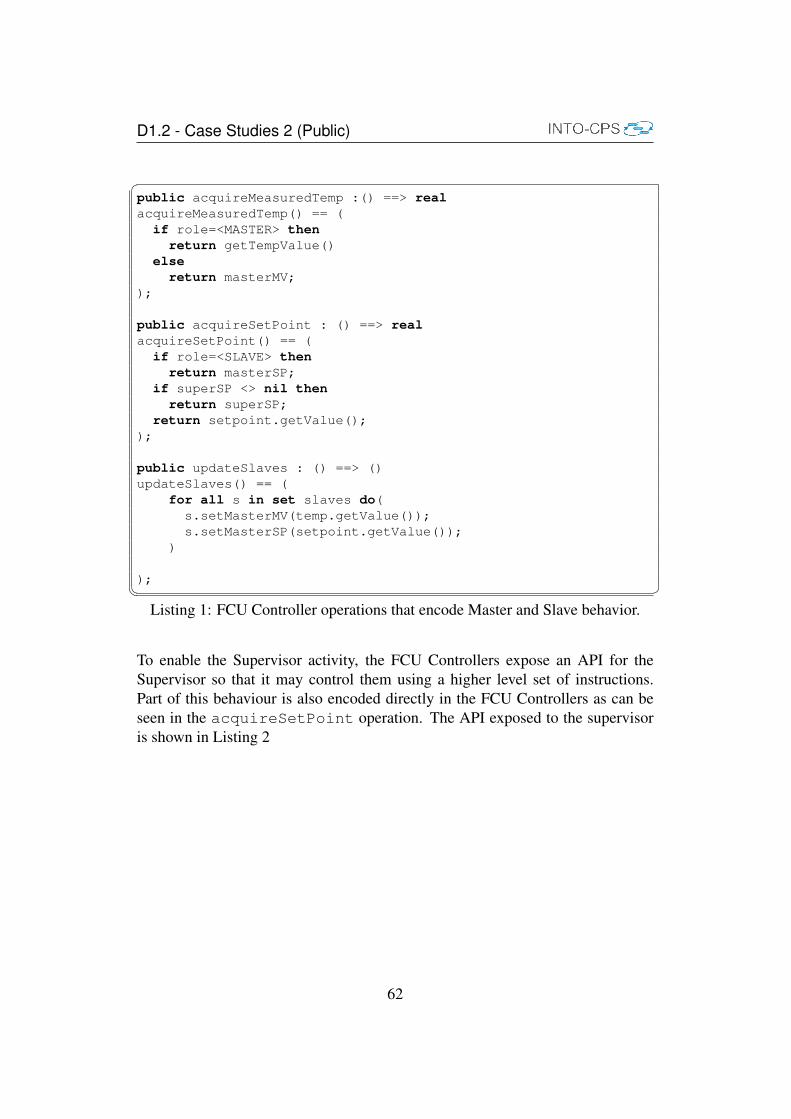
D1.2 - Case Studies 2 (Public)
�public acquireMeasuredTemp :() ==> realacquireMeasuredTemp() == (if role=<MASTER> thenreturn getTempValue()
elsereturn masterMV;
);
public acquireSetPoint : () ==> realacquireSetPoint() == (if role=<SLAVE> thenreturn masterSP;
if superSP <> nil thenreturn superSP;
return setpoint.getValue(););
public updateSlaves : () ==> ()updateSlaves() == (
for all s in set slaves do(s.setMasterMV(temp.getValue());s.setMasterSP(setpoint.getValue());
)
);� �Listing 1: FCU Controller operations that encode Master and Slave behavior.
To enable the Supervisor activity, the FCU Controllers expose an API for theSupervisor so that it may control them using a higher level set of instructions.Part of this behaviour is also encoded directly in the FCU Controllers as can beseen in the acquireSetPoint operation. The API exposed to the supervisoris shown in Listing 2
62

D1.2 - Case Studies 2 (Public)
�public setSuperSetPoint : real ==> ();
public promoteToMaster : set of Controller ==> ();
public demoteToSlave : () ==> ();
public turnOff : () ==> ();
public getRole : () ==> Role
public getSlaves : () ==> set of Controller
public getSPValue : () ==> real� �Listing 2: FCU Controller operations that form the API exposed to the Supervisor.
CT Model of Building and HVAC System The building and HVAC model im-plemented for the year 2 case study describes a 140m2 floor in an office buildingsupplied by a hydronic system in heating mode. The HVAC system is made of aHP providing hot water to the FCUs in the occupied space and to the AHU respon-sible for maintaining fresh air requirements in the zones. The floor is supplied byfour FCUs; one for each individual room and two complementing each other toserve a large zone. The thermal performance of the building is reasonable leadingto a thermal demand of about 50 kWh/m2/year. This performance is based ontypical northern Europe climate conditions.
Modeling the complexity of the integrated system was not possible in OpenMod-elica (OM). Fluid flow and heat transfer phenomena induced by the system com-ponents are not currently supported by OM. Instead the project team used Dymola2016, which supports FMI 2.0. Dymola is commercial tool, based on Modelica,for modeling and simulation of integrated and complex systems. It is a multi-engineering tool widely used in automotive, energy systems, and aerospace appli-cations. A schematic overview of the CT model is illustrated in Figure ??. Theseare complex models that take into account solar radiation and occupancy levels inthe building and maintain acceptable levels of water and air pressures as per man-ufacturer specifications. The model has 8 inputs being the fan speed and valveopening position of each of the four FCUs and 4 outputs being the actual roomtemperature of each room and area measured at the FCU level.
The indoor temperature in each room is controlled using an FCU device, wherethe FCU uses a water coil and fans to heat or cool the circulated air inside eachroom. The air Handling Unit (AHU) supplies fresh air to each FCU, while theHeat Pump (HP) supplies hot or cold water to the water coils in the FCU. The
63

D1.2 - Case Studies 2 (Public)
Table 5: Statistics of CT FMU generated from Dymola
Item StatisticsConstant 7373 scalarsFree Parameters 6101 scalarsParameters depending 5738 scalarsInputs 8 scalarsOutputs 4 scalarsContinuous time-states 300 scalarsTime-varying variables 4635 scalars
water that flows into the coil is pressurized by the HP, whereas a Fan blows thecirculated room air through the coil to regulate the indoor air temperature. AnFCU PI-controller regulates the fan speed and the rate of the water flow from theheat pump to the coil in order to maintain a set temperature in the room in whichthe FCU is located.
The model is based on mass and energy balances in a given room/zone. Two majorassumptions were used to simplify the model for a given zone:
• The zone air is well mixed at all times
• Long wave radiation exchange between surfaces is ignored
The model is compiled in Dymola 2016 using FMI export and selecting the fol-lowing options: model exchange including source code and 64-bit binaries. Thisis the only export option that is currently compatible with the INTO-CPS COE.The complexity of the generated FMU is summarized in Table 5.
Code Generation Proceeding to code generation, after incorporating the neces-sary tools required for the targeted hardware platform (e.g. the distributed FCUunits and the supervisor), the code will be generated based upon the developedmodels as described in the previous sections. Those will describe the overall be-havior of the FCUs, communications and supervision of them. For the targeted3 FCUs mainly, for the 2 areas in the zone and room 2, the embedded devicewill be based on a 16-bit PIC24FJ embedded micro-controller. In order to exciteadvanced controller and prognostics capabilities for several FCU operations (e.g.controlling the Fan motor), we incorporate the Zynq Platform motor controller forroom 1. Zynq 7000 consists of 2 A9 ARM processors and a XilinX FPGA. Fi-nally the supervisor will be flashed to the Zybo platform (similar to Zynq) whichfor now is handling FCU set points provided to the rooms. Connections from the 3PICs and the Zynq platform with the Zybo Supervisor are being handled throughUART cable. The year 2 current hardware setup is shown in Figure 32.
64

D1.2 - Case Studies 2 (Public)
Figure 32: Hardware Setup for Year 2 case study towards code generation
We have extracted a proof of concept version of the PI controller regulating the fanand valve modules of the FCU, based on the sensed room air temperature. For theroom 2 instance, as shown in Figure 32 a proof of concept PI controller modeledin Overture using VDM (example taken from year 1 use case) has generated the Ccode for the 16-bit PIC embedded micro-controller. Code has been refined in orderto meet hardware platform characteristics of the PIC architecture. Compilationand flashing of the C code to the micro-controller was successful, executing basiccontroller commands. Currently automated code generation for the distributed
65

D1.2 - Case Studies 2 (Public)
case is not supported. Results from the code compilation and flashing to the PICmicro-controller have accumulated an 8.6% (706 bytes) usage of data memoryutilized by the PID controller, while the program data used to realize the controlleroperations is accumulated at 38.1% (50049 bytes).
5.4 HVAC Co-simulation Results
In this section we describe co-simulation results for several HVAC scenarios forthe building case study, based on the INTO-CPS platform. Our focus will be onthe design and evaluation of the control algorithms deployed both on the Fan CoilUnits (FCUs), the Supervisor and the Air Handling Unit (AHU) for the Year 2 casestudy. Co-simulation will based on FMUs generated from the models describedin the previous sections; we define different scenarios for which we configure ourco-simulation parameters in order to evaluate control functionality of the HVACsystem as a whole. Table 6 outlines the co-simulation experimental setup for thedifferent scenarios evaluated within our Year 2 models.
Table 6: Scenario Experimental Setup: Control Operation in Variable Tempera-ture conditions
FMUs 2 FMUs with 4 connections (1 encrypted) INTO-CPSConnections inputs, outputs JSON file created by ModelioDE 1 FMU describing functionality of 4 FCUs and Supervisor OvertureCT 1 FMU describing functionality of rooms and AHU DYMOLATotal Experiment Variable Step Size [0.5 - 60]: 4000 sec INTO-CPSScenario 1 Environmental conditions (OAT) remain unchangedScenario 2 Outside Air Temperature (OAT) DecreasesScenario 3 Outside Air Temperature (OAT) Increases
Scenario 1: Evaluate Controls Operation in normal conditions
For scenario 1 the CT and DE FMUs are co-simulated in normal temperatureconditions. In this case, the thermal effects of room materials, air-mass flow char-acteristics and external environmental conditions are mapped by the CT and DErepresentations as described in previous sections.
Figure 33 shows the behavior of different controlled variables of the model, suchas room air temperature (RAT), of all the 4 rooms defined in our use case. Theroom air temperature set point is considered constant at 294.5K (21.5 oC) andcommunicated by the CT model to each FCU controller. Each FCU controllerregulates the valve position and fan speed to manipulate the Entering Water Tem-perature (EWT) and Supplied Air Temperature (SAT), respectively for each room.We observe the controls operation leading to the steady temperature increase from
66

D1.2 - Case Studies 2 (Public)
Figure 33: Scenario 1 INTO-CPS Co-simulation Results for Room 1, Room 2 andZone (Area 1 and Area 2): Normal Operation
the initial value. Both rooms and the zone temperatures set-points are not reachedjustifying the continuous increase of the temperature for the whole duration of theco-simulation, shown in Figure 33.
Scenario 2: Evaluate Control Robustness when temperature values radicallydecrease due to environmental changes
The co-simulation results allow for visualization and post processing of variousparameters of interest in building applications such as room air temperature, walltemperature, FCU valve opening, FCU fan speed, and controller output. Theseparameters can be used to calculate a number of indexing quantities to evaluatebuilding performance that for this normal scenario, are comfort and energy con-sumption. That is the reason why the PI controller – modeled in VDM-RT – triesto reduce the distance between the initial room temperature set point and the realtemperature (RAT) by regulating valves (for heated/cooled water flow) and Fan(warm/cold air), until the distance between them equals zero.
67

D1.2 - Case Studies 2 (Public)
Figure 34: Scenario 2 INTO-CPS Co-simulation Results for Room 1, Room 2 andZone (Area 1 and Area 2): OAT decreases
Figure 34 shows the temperature when outside air temperature is radically changed(OAT ↓) for Scenario 2. We evaluate the controller robustness when the buildingis exposed to sudden changes in the outside air temperature (OAT). In particularthe OAT was subject to a step function decrease of 20 oC from its normal valueof 5 oC. Figure 34 depicts the building response to this sudden change. Presentedvariables are the room air temperatures and valve openings.
5.5 Industrial Needs and Assessment
In this section we proceed with the second assessment of the requirements asshown in Table 7 evaluating the INTO-CPS platform as described above. Ini-tial requirements are defined according to core functionality for the Year 2 usecase.
68
D1.2 - Case Studies 2 (Public)
5.6 UTRC-Req-001: Simulation Completeness
• DescriptionINTO-CPS baseline tools must offer simulation completeness (for continu-ous, discrete and co-models) based on the allowable modeling parametersselected by the end-user. Completeness will be assessed with respect toco-simulation platform functionality (crashes, logging and run-time errors)during execution of co-simulations.
• Related to Baseline Tools RequirementsRequirements 0003-0005 are related because the modeling of the time stepcould be done at discrete, continuous and co-simulation level
• Method of VerificationFor all co-simulations executed by UTRC stuff, we successfully co-simulatedthermal, air and physical components through FMUs extracted by Dymola.Discrete FCU controllers were modeled in Overture from which FMUs alsohave been extracted. Co-simulation results are considered to be complete.
• Assessment: AchievedIn all of our models in the Year 2 case study, the simulation completenesswas shown using the INTO-CPS platform. Indicator: 100%
5.7 UTRC-Req-002: Simulation Delays
• DescriptionINTO-CPS platform should execute simulations by providing extra time de-lays at minimum. With extra time delays we describe simulation executionswhere simulation solvers might exhibit various delays into acquiring results.
• Related to Baseline Tools RequirementsRequirements 0003-0005 are related because the modeling of time stepcould be done at discrete, continuous and co-simulation level
• Method of VerificationFor the Year 2 case study and the CT and DE models, simulation delayswere negligible for all the co-simulations performed. Some delays occurredwhen selecting a fixed point co-simulation step size which has been reportedto the project consortium
• Assessment: AchievedIn all of our models in the building case study, no simulation delays were
69

D1.2 - Case Studies 2 (Public)
encountered when executing co-simulations using FMUs from both Dymolaand Overture. Indicator:95%
5.8 UTRC-Req-003: Design Space Exploration
• DescriptionDesign space exploration techniques should be applied to both continuousand discrete models when executing a series of simulations
• Related Baseline Tools RequirementsRequirements 0018-0020 could be necessary in order to assess the maxi-mal/minimal value from a range of parameters.
• Method of VerificationThis requirement should be verified using simulations and functional test-ing. Currently there is not support for design space exploration within thebaseline tools. Early design state exploration experiments have been appliedoffline in the building case study independently from the tools evaluated inthis report.
• Assessment: not achieved Currently the design space exploration (DSE) isnot supported within the INTO-CPS toochain. CT and DE model evaluationstarted but not completed. Indicator:25%
5.9 UTRC-Req-004: Simulation Accuracy and Precision
• DescriptionINTO-CPS should be able to provide a varied level of simulation accuracywith a user-selected variable precision. This will increase confidence inresults from co-simulation executions
• Related Baseline Tools RequirementsRequirements 0045, 0047, 0055, 0058, 0061, 0065 : Semantics are nec-essary in order to keep accuracy and confidence. Quantifiable simulationtolerance of the INTO-CPS co simulation are necessary to keep accuracy.
• Method of VerificationHaving in place formal semantics for INTO-CPS baseline tools is of paramountimportance in order to enable simulation accuracy and precision. CurrentlyINTO-CPS tools have a limited support with respect to simulation and co-
70

D1.2 - Case Studies 2 (Public)
simulation manipulation (e.g. rollback or test case evaluation) with accurateresults.
• Assessment: partially achievedIn the current evaluation study, tools have depicted certain levels of preci-sion in the simulation experiments. This includes variable step co-simulationartifacts (e.g. raw cosimulation data, graphs) generated by the orchestrationengine and the INTO-CPS application. We expect to increase simulation re-sults accuracy (using time-tags, debugging log files, memory consumption)in co-simulation in the next year of the INTO-CPS project. Indicator:40%
5.10 UTRC-Req-005: Scalable Simulation
• DescriptionINTO-CPS platform should adequately produce simulation results in largecontinuous, discrete or co-models where complexity is significantly high.
• Method of VerificationAlthough this requirement is often bound to the available resources, fromthe co-simulation engine point of view, the INTO-CPS toolchain should beable to produce simulation and co-simulation results for a certain level ofmodel complexity. As this verification will depend on the model complex-ity we argue that the specific requirement will be re-evaluated in year 3 ofINTO-CPS project.
• Assessment: partially achievedIn the current Year 2 evaluation, INTO-CPS platform has exhibited certainlevels of simulation efficiency when tackle a certain level of model com-plexity, particularly for our CT model. This may include solver evaluationand assessment during fixed or variable step co-simulations, from the INTO-CPS toolchain. Indicator:60% achieved
5.11 UTRC-Req-006: Code generation
• DescriptionINTO-CPS platform should allow code generation with respect to selectedhardware in certain programming languages (e.g. C ) automatically fromthe models.
• Related Baseline Tools RequirementsRelated to requirements 0037, 0042, 0044.
71

D1.2 - Case Studies 2 (Public)
• Method of VerificationCode generation from the VDM-RT model on PIC micro-controllers (UTRCFCUs) for executing FCU PI commands
• Assessment:partially achievedINTO-CPS code generation support is not yet mature particularly for theOverture tool where we model our supervisor and the PI controllers. Proofof concept results have been shown for basic PI FCU controller in the se-lected hardware platform but not configured for the distributed case. Indi-cator:30%
5.12 UTRC-Req-007: Platform Independence and FMU sup-port
• DescriptionINTO-CPS platform should be independent from external tool dependenciesand support FMI-based cosimulation (version 2.0) for both encrypted andplain FMUs.
• Related Baseline Tools RequirementsNew requirements.
• Method of VerificationEvaluate both encrypted and non-encrypted FMUs’ cosimulations;
• Assessment:partially achievedMajor contribution of the INTO-CPS platform being used from the web-app. Still there is a certain level of matureness that can be achieved in year3. Indicator:70%
5.13 Conclusion - Reporting Experiences
The goal of this deliverable was to bring insights about industry benefits and weak-nesses of using INTO-CPS platform, and to plan for the next technological ad-vances of INTO-CPS features according to the project planning for Year 3. Byevaluating our HVAC controllers through different co-simulation scenarios, weare in the position to adjust and refine INTO-CPS tools requirements, providingvaluable feedback to the consortium. We discuss below and reflect our experi-ences of working with FMI-based tool chains for the design and development ofCPSs.
72

D1.2 - Case Studies 2 (Public)
Tabl
e7:
UT
RC
’sre
quir
emen
ts
Req
.C
ateg
ory
Sub
Cat
.In
sigh
tPr
iori
tySt
atus
Vers
ion
Ass
ess
UT
RC
-Req
-001
Non
-Fun
ctio
nal
Syst
emSi
mul
atio
nC
ompl
eten
ess
MY
ear1
1ac
hiev
ed,1
00%
UT
RC
-Req
-002
Non
-Fun
ctio
nal
Syst
emSi
mul
atio
nD
elay
sS
Yea
r11
achi
eved
,95%
UT
RC
-Req
-003
Non
-Fun
ctio
nal
Effi
cien
cyD
esig
nSp
ace
Exp
lora
tion
CY
ear1
1no
tach
ieve
d,25
%U
TR
C-R
eq-0
04N
on-F
unct
iona
lTo
ols
Sim
ulat
ion
Acc
urac
yan
dPr
ecis
ion
CY
ear1
1Pa
rtia
lly,4
0%U
TR
C-R
eq-0
05N
on-F
unct
iona
lTo
ols
Scal
able
Sim
ulat
ion
SY
ear1
1Pa
rtia
lly,6
0%U
TR
C-R
eq-0
06To
ols
Scal
abili
tyC
ode
Gen
erat
ion
SY
ear1
1Pa
rtia
lly,3
0%U
TR
C-R
eq-0
07Fu
nctio
nal
Soft
war
ePl
atfo
rmIn
depe
nden
cean
dFM
Usu
ppor
tS
Yea
r11
part
ially
achi
eved
,70%
73

D1.2 - Case Studies 2 (Public)
• It is important for a project to have a common CPS design description that iscentral and shared by all project members. This design should evolve overtime but these evolutions should be visible and agreed upon by all members.Ideally, this design should be enforced through distribution and adherenceto constituent model specifications through FMI model descriptions. Wherethe tools do not mandate this, it should be project policy to do so nonethe-less. Tools that do not support importing of FMI model descriptions shouldnot be avoided if at all possible.
• To combat undocumented assumptions slipping through the FMI tool chain,all restrictions, units and other kinds of assumptions must be properly docu-mented. Ideally, this should be done in the main design document or SysMLmodel. If this is not possible, an independent document containing the as-sumption should be created. This document must be shared and accessibleby all partners. From a tooling perspective, such assumptions should beencoded in the constituent models and the FMI interface.
An important aspect was as well the need for specific INTO-CPS features suchas design space exploration and code generation which will elevate the platformefficiency towards scalability and SiL/HiL simulations respectively. As next stepsin Year 3 of the INTO-CPS we anticipate to apply INTO-CPS technologies in or-der to analyze more complex HVAC cases in order to evaluate scalability of theorchestration engine. Having in mind current state-of-the-practice commercialco-simulation platforms we aim to evaluate new HVAC industrial needs throughINTO-CPS features including mature code generation for SiL and HiL simula-tions, design space exploration and model checking.
6 Automotive Case Study
6.1 Specifications
The main goal for the automotive case study in INTO-CPS is to create a tool forrange prediction of electric vehicles. This shall be done by simulating the drivetrain of the electric vehicle and other relevant electric auxiliary loads such as theair conditioning, while integrating information from weather, topography or traf-fic. The range optimization assistant shall enable the driver of an electric vehicleto select a route which offers the maximum range of the vehicle with the givenelectric battery, in order to alleviate the drawbacks of the limited range.
For the initial case study (see also deliverable D1.1a [HLB+15]), we distinguish
74

D1.2 - Case Studies 2 (Public)
between two scenarios :
• Offline: A user gives as input a desired start and end destination. A specificroute is simulated and the energy consumption is calculated.
• Online: The online mode is activated as soon as a route was chosen andthe car starts moving in a certain direction. In this situation, real-time datacoming from the vehicle like torque requirements, current speed, availablebattery power (state of charge) etc can be accessed.
Here the following factors play an important role in the work flow:
1. The state of the car (state of charge of the battery) is updated period-ically . If the energy level deviates from the prediction (done in theoff-line mode) and the energy level isn’t enough to reach the destina-tion another route is simulated. If no route is found under the energyconstrains the user is alerted. If a new route was found the user isalerted and has to choose whether the route should be updated.
2. The environment (weather or traffic situation has changed) is seen as atrigger that causes a new simulation to start and generate another route.The user has to actively agree upon the old route being overwritten bythe newly generated route.
3. The driver deviates to another route and thus triggers a new route thatneeds to be generated. Automatically, the old route is overwritten bythe new route .
An illustration of the triggers inside the system is shown in figure 35 below.
Figure 35: Alert system of the case study.
To demonstrate the alert system the following situation will be shown in the casestudy. The driver starts the application and enters a destination. The system re-turns the optimal route. Now there are three possible scenarios:
1. The weather situation changed and a new Route A is the better one.
75

D1.2 - Case Studies 2 (Public)
2. Nothing happens and the driver arrives at the destination.
3. The traffic situation has changed and a new Route C is the better one.
These scenarios are depicted in the following figure 36.
Figure 36: Scenarios for selection of different routes depending on the differentalerts.
The alarm system is described in more detail below, and was implemented as aprototype by the end of year 2.
6.2 Specification of the HiL scenario
In order to increase the level of complexity of the automotive case study, a HiLscenario is proposed that goes beyond the originally planned scenario. The goalof this is to better evaluate the INTO-CPS tools, by developing and optimizing thegas pedal controller (see below) with the help of the INTO-CPS tools.
This setup contains the following components that will be described below. It par-tially builds on top of a setup for a driving simulator that was used in the HoliDesresearch project (see for example http://www.holides.eu/content/adapted-automation-adcos-video-dlr-twt-ibeo):
Driver: A person interacting with the driving simulator by means of pedals (brakeand accelerator) and steering wheel. As we only consider the longitudinal dy-namics in the case study, only the gas and brake pedal are relevant for this sce-nario.
76

D1.2 - Case Studies 2 (Public)
Figure 37: Schematic scenario for the automotive case study with a HiL setting.
Steering Wheel and pedals: The Human-Machine-Interface consists of a physi-cal steering wheel and a gas and braking pedal (Logitec G27 Racing Wheel).
Controller: A controller (here to be implemented on a Raspberry Pi micro-controller) that uses as input the gas pedal signal and modifies this signal forthe output, based on parameters provided by vehicle simulation. The controllerimplements an algorithm that calculates the parameters for modification of the gaspedal signal. Based on the remaining range or the SoC level, the output level ofthe gas pedal is reduced. This controller, and in particular its function for adaptingthe gas pedal curve, has to be developed from scratch. This will be done using theINTO-CPS tools. An initial proposal for this function can be seen below in Figure38. There, the output of the controller is initially equal to the input. Dependingon the state of the vehicle, this curve can be modified by the controller, such thatthe output is lower than the input and the gas pedal is ”softened”. When the inputis at its maximum (i.e. the driver requests full acceleration), the output must alsoreach the maximum, since it can be crucial for the driver’s safety.
Virtual reality simulator: A complete setup for a driving simulator is based onthe OpenDS simulation (see www.opends.eu).
Vehicle simulation: The bulk of the simulation that has been developed so farin INTO-CPS (see [HLB+15]). The input signals for the vehicle simulation are
77

D1.2 - Case Studies 2 (Public)
generated by the VR simulator in form of velocity, position of the car, or acceler-ation. Input signals such as temperature or atmospheric pressure are generated bythe weather module based on the current car position.
Feedback: A visual signal, in form of a simple LED that changes its color is givento the driver in the attempt to influence his driving behavior to improve range andpower efficiency. The LED turns green every time the driver accelerates slowlyand in case of a kick-down or a sudden push of the gas pedal the LED will turnred.
Figure 38: Output of the gas pedal controller, as a function of the input. Ini-tially the output is equal to the input (black diagonal line), but depending on theremaining range of the vehicle, the curve can be ”softened” (gray lines).
Of these components, mainly the feedback and the controller need to be devel-oped, using the INTO-CPS tools. The other components already exist, but need tobe adapted.
6.3 Model
The system model consist of the following parts:
78

D1.2 - Case Studies 2 (Public)
• Longitudinal dynamics of an electric vehicle, including the battery and airconditioning
• Route planning including traffic information
• Ambient conditions
• Alarm System
These models are coupled with the INTO-CPS Co-Simulation Orchestration En-gine (COE). Most of these models are described in detail in the previous deliv-erable [HLB+15], and their description will not be repeated here, for the sake ofclarity. Since the CT models of the automotive case study are written in Matlab,a Matlab-FMU wrapper had to be developed by TWT, that allows coupling of themodels to the COE (see also Deliverable D6.2 [KFP+16]).
The SysML connections diagram for the multi-model, consisting of the routemodule, the weather module and the longitudinal dynamics module (internallycalled ”ArtSim”) is shown in Figure 39 below.
Figure 39: SysML Connections diagram including the longitudinal dynamics, theweather module and route module.
79

D1.2 - Case Studies 2 (Public)
6.4 Route module (CT)
During year 2, the route module that was previously described in DeliverableD1.2e [KB15] was improved. Now, it takes the current position and velocity (cal-culated from the longitudinal dynamics) as input for the next section of the route(this is also shown in the connections diagram in Figure 39). This in turn makesthe whole simulation more realistic, as it smoothes the acceleration curve.
6.5 Alarm System (DE)
We consider a controller, which we call an alarm system, with the function tomonitor the state of the vehicle, in terms that are relevant for the route assistantthat is developed in this case study. It consists of four functions which monitor thestate of the battery (i.e. the SoC), the traffic, the weather and the route. If any ofthese changes, the simulation is reset, to take the changed conditions into account.It is foreseen to use real data in the long run, but for developing this alarm system,simulated data can be used. The state diagram of this alarm system is displayedin figure 40.
The default state is SignalMonitoring, in which the alarm system continuouslychecks the vehicle parameters. If any of these is out of its boundaries, the Co-Simulation is re-started. If the driver decides to take a different route than theproposed one, the route needs to be calculated before these values then are handedover to the weather module, for delivering the weather values to the Co-Simulation.A sudden change in weather conditions also triggers the restart of the weathermodule, and in consequence of the Co-Simulation. If the measured velocity ofthe vehicle is on average significantly lower than the planned velocity, a trafficjam is assumed, which requires a re-start of the Co-Simulation as well. Finally,if certain vehicle parameters (such as the battery SoC) suddenly change, the newvalues need to be taken into account.
The alarm system is being implemented in VDM and coupled to the COE as anFMU. At the time of writing this deliverable, this is still work in progress.
6.6 Simulation results
To simulate the range-prediction, a route in the vicinity of Stuttgart (Germany) isselected. The route has a length of approximately 34km and is largely on countryroad. The height profile is depicted below in Figure 41. Initially, the road has a
80
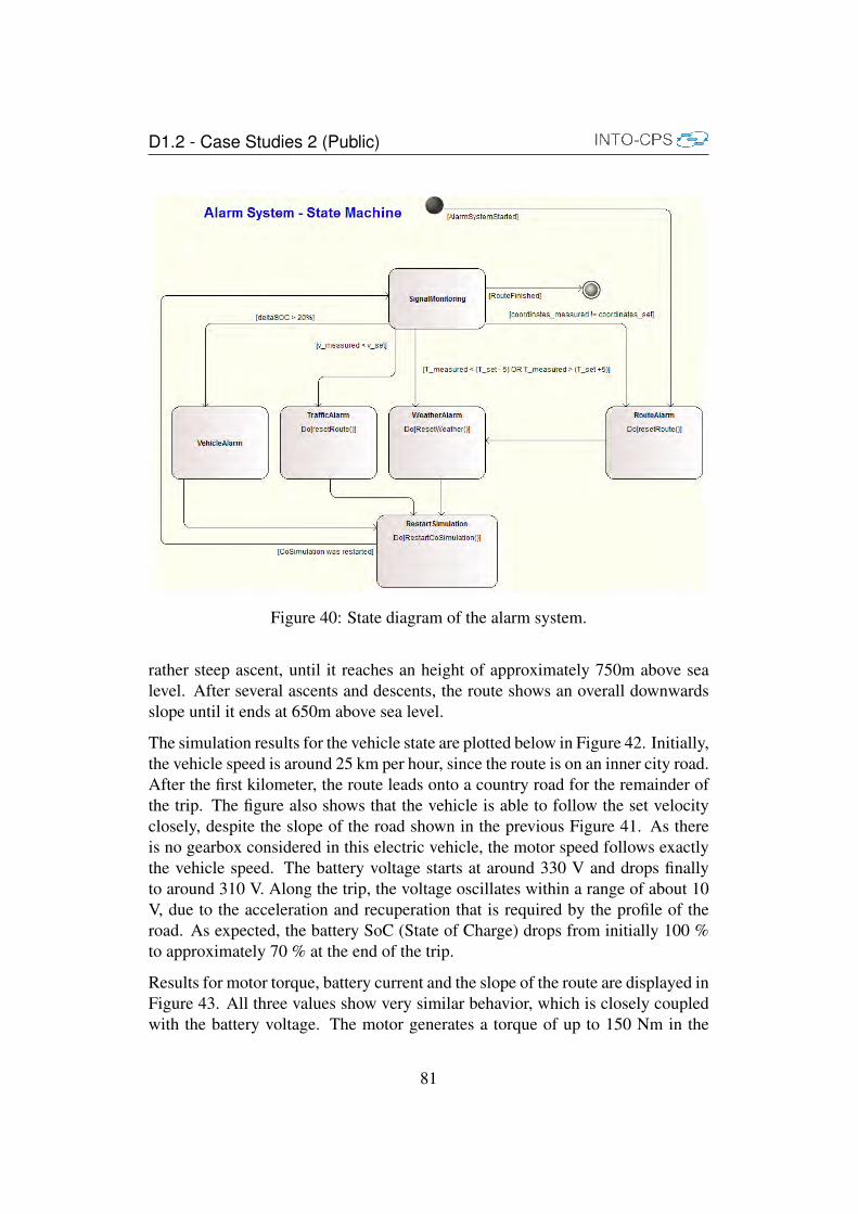
D1.2 - Case Studies 2 (Public)
Figure 40: State diagram of the alarm system.
rather steep ascent, until it reaches an height of approximately 750m above sealevel. After several ascents and descents, the route shows an overall downwardsslope until it ends at 650m above sea level.
The simulation results for the vehicle state are plotted below in Figure 42. Initially,the vehicle speed is around 25 km per hour, since the route is on an inner city road.After the first kilometer, the route leads onto a country road for the remainder ofthe trip. The figure also shows that the vehicle is able to follow the set velocityclosely, despite the slope of the road shown in the previous Figure 41. As thereis no gearbox considered in this electric vehicle, the motor speed follows exactlythe vehicle speed. The battery voltage starts at around 330 V and drops finallyto around 310 V. Along the trip, the voltage oscillates within a range of about 10V, due to the acceleration and recuperation that is required by the profile of theroad. As expected, the battery SoC (State of Charge) drops from initially 100 %to approximately 70 % at the end of the trip.
Results for motor torque, battery current and the slope of the route are displayed inFigure 43. All three values show very similar behavior, which is closely coupledwith the battery voltage. The motor generates a torque of up to 150 Nm in the
81

D1.2 - Case Studies 2 (Public)
Figure 41: Height profile of the selected route.
steep sections of the road. Accordingly, a current of up to 200 A is drawn fromthe battery, in particular in those sections that have a slope of up to 20 %.
The temperatures that are calculated from the air conditioning module (for a moredetailed description of this model, see Deliverable D1.1e [KB15]) are displayedin Figure 44. Initially, the temperature of the air inside the vehicle is 20 C, whilethe temperature outside is 5 C (e.g. when the vehicle was parked in a garage inwinter). The setpoint for the temperature controller is 23 C. While the temperatureof the air inside the vehicle quickly rises, the fixtures (e.g. the seats) only heat upslowly. At the same time, the temperature at the windows and at the vehicle casedrops quickly and reaches a steady state at 7 C.
6.7 Evaluation of INTO-CPS tools
In this section, the evaluation of the emerging INTO-CPS tools from the autmo-tive’s case study’s perspective is given.
• Modelio
The SysML diagrams for describing the system model that were generated
82

D1.2 - Case Studies 2 (Public)
Figure 42: Simulation results for vehicle speed, motor speed, battery voltage andSoC.
in Modelio in year 1 were transferred to Architectural diagrams and Con-nection diagrams, to make use of the INTO-CPS extensions of Modelio.Exporting a COE configuration from this Connections diagram (see for ex-ample Figure 39) makes the process easier than manual configuration of theCOE, and less error prone.
83

D1.2 - Case Studies 2 (Public)
Figure 43: Simulation results for motor torque, battery current and slope of theroute.
Figure 44: Simulation results for temperatures inside and outside the vehicle.
• VDM / Overture
A simple version of the Alarm system (see section 6.5) was implemented
84

D1.2 - Case Studies 2 (Public)
in Overture. Using the new FMU export option, this model was exportedto an FMU and connection to the COE (i.e. coupling the alarm systemto the remainder of the models) is being performed at the time of writingof this deliverable. The new FMU export option in Overture significantlysimplifies the process. In combination with the import of the MODELDE-SCRIPTION.XML from Modelio, the whole workflow is integrated further,and errors (e.g. due to different naming of signals) are reduced.
• Co-Simulation Orchestration Engine / INTO-CPS application
The different simulation models were coupled with the COE, using theINTO-CPS application. The configuration of the multi-models was createdfrom Modelio, and the Co-simulation was configured in the INTO-CPS ap-plication. The INTO-CPS application is user-friendly and rather simple touse, which makes the shift to this tool quite simple. Throughout year 2 ofINTO-CPS, the COE has become more stable, which improved usability.
Im summary, the core parts of the emerging INTO-CPS tools and workflows wereused and evaluated in the automotive case study. The integrated tool-chain of-fers many benefits for a smooth workflow. The fact that the tool-chain is open toother tools that support the FMI standard (such as Matlab) allows re-using exist-ing know-how, and is therefore a great advantage for potential users. Feedbackwas given from the automotive case study to the tool developers regarding user-experience, requirements and potential bugs.
6.8 Requirements and Assessments
6.8.1 TWT 1: Validity checking
• Description: The validity of system models, i.e. the correctness of the con-nected input and output signals to and from the different models is checkedby the tools.
• Method of Verification: Manual variation of input and output signals tocheck if the tools detect the changes. If the tools notify the user of a mis-match, this requirement is fulfilled.
• Assessment: Complete. The INTO-CPS application detects if the name ofa input / output signal is false, and gives a warning to the user.
• Related baseline tools requirements: 0035 - 0036
• Degree of achievement: 100%
85

D1.2 - Case Studies 2 (Public)
6.8.2 TWT 2: System structure
• Description: A system structure, describing the connections between thedifferent models and their hierarchy, is created and saved by the tools, inorder to re-import and modify later. This simplifies the generation, distribu-tion and modification of the whole system architecture.
• Method of Verification: Manual generation of a system model to importinto the tools. If the system structure is correctly imported, this requirementis fulfilled.
• Assessment: Complete. The INTO-CPS application allows saving of com-plete projects, including their hierarchy. SysML diagrams, describing thearchitecture of the system, can also be exported.
• Related baseline tools requirements: 0001, 0005, 0012
• Degree of achievement: 100%
6.8.3 TWT 3: Results tracing
• Description: Simulation results are traced to the requirements and the mod-els where the results originated from. This makes testing of the require-ments easier and thus increases trust in the simulation results.
• Method of Verification: Comparison of results and requirements in simplemodels. For a measurement, the number of requirements that are linked tosimulation results can be compared to the total number of requirements.
• Assessment: Not started. The INTO-CPS tools do not yet support trace-ability functions.
• Related baseline tools requirements: 0015 - 0017
• Degree of achievement: 0%
6.8.4 TWT 4: Requirements assessment
• Description: An indicator is provided to determine how well a requirementhas been met, not just yes/no.
• Method of Verification: Requirements can be varied systematically to as-sess if the resulting indicator / ranking function reacts accordingly.
86

D1.2 - Case Studies 2 (Public)
• Assessment: Not started. The INTO-CPS tools do not yet provide the trace-abilty between requirements and results.
• Related baseline tools requirements: 0021
• Degree of achievement: 0%
6.8.5 TWT 5: System creation from SysML
• Description: Starting from a SysML model of the system, a skeleton sys-tem model (in FMI) is created. This will simplify the workflow by connect-ing the different tools for system modelling and simulation.
• Method of Verification: Comparison of an automatically generated skele-ton system model with its SysML model.
• Assessment: Complete. The INTO-CPS profile for Modelio offers exportof FMI modelDescription.xml files.
• Related baseline tools requirements: 0049
• Degree of achievement: 100%
6.8.6 TWT 6: Version checking
• Description: The tools should be able to check if the interfaces betweendifferent models have changed due to different versions. This is relevant forthe development process of modelling, especially when different parties areresponsible for different models.
• Method of Verification: Selection of different model versions with dif-ferent inputs and outputs. If different versions of the same model can beselected, or the user is notified of differences between model versions, thisrequirement is fulfilled.
• Assessment: Ongoing. The INTO-CPS application detects if input / out-put signals do not match the corresponding names. However, versioningsupport is not yet implemented.
• Related baseline tools requirements: 0090
• Degree of achievement: 80%
87
D1.2 - Case Studies 2 (Public)
6.8.7 TWT 7: Version selection
• Description: The user selects different versions of the same model (eithersingle model or system model).
• Method of Verification: Provided / not provided.
• Assessment: Not started.
• Related baseline tools requirements: It remains to be discussed if thisrequirement will be incorporated in the general requirements document, de-liverable D7.5 [LPO+16].
• Degree of achievement: 0%
6.8.8 TWT 8: Parameter variation
• Description: Model parameters are systematically and automatically variedwithin defined limits. This allows systematic optimization of the models.
• Method of Verification: Provided / not provided.
• Assessment: Not started. Design Space exploration functions are still underdevelopment and have not yet been tested with this case study.
• Related baseline tools requirements: 0020
• Degree of achievement: 0%
6.8.9 TWT 9: Parameter selection
• Description: If the user wants to parametrize a whole model at once, pa-rameter sets for models are selected from a parameter file. This can behelpful if relatively complex models have large parameter sets, describingfor instance different variants of a product.
• Method of Verification: Provided / not provided.
• Assessment: Not started.
• Related baseline tools requirements: It remains to be discussed if thisrequirement will be incorporated in the general requirements document, de-liverable D7.5 [LPO+16].
• Degree of achievement: 0%
88

D1.2 - Case Studies 2 (Public)
6.9 Conclusion
In this part, the progress of the automotive case study that was made during year 2is presented. Based on the know-how that was already available, TWT has createda co-simulation using CT models and have started with DE modeling, to create acruising range prediction tool for electric vehicles. This tool takes into accounta model of the physical behaviour of the vehicle (the longitudinal dynamics, thebattery, electric engine and the air conditioning) as well as the topology of thechosen route, and weather conditions (relevant for the air conditioning) and asystem for monitoring the state of the vehicle. It will therefore allow the user topredict the remaining battery charge, based on on realistic data (vehicle physics,route, weather). It can be used for example for realistic calculation of electricvehicle fleets or for integration in the vehicle’s software, as an addition to thenavigation system, or for optimizing vehicle settings for maximum range.
The focus of this year’s work was the transfer of the case study to the INTO-CPS tool-chain. This primarily meant usage of the COE, and as a consequence,connecting the Matlab models in a FMI-compliant fashion. To achieve this, aMatlab FMU wrapper was developed during year 2. Furthermore, integration ofthe workflow from the abstract system models (in SysML) to creation of a Co-simulation configuration, was achieved.
To further develop the case study, a HiL scenario is specified in this deliverable.This will be largely based on existing technologies, and serve to evaluate moreaspects of the INTO-CPS tool-chain, such as code generation or design spaceexploration.
The evolving INTO-CPS tools will be further evaluated in the third year. One fo-cus here will be the evolving functionalities regarding traceability, which are veryinteresting for Systems Engineering applications. In terms of implementation, theHiL scenario that is described in this document will be the main effort in year 3,along with the assessment of the requirements.
89

D1.2 - Case Studies 2 (Public)
References
[CLJ15] Martin Peter Christiansen, Peter Gorm Larsen, and Rasmus NyholmJørgensen. Agricultural Robotic Candidate Overview using Co-modelDriven Development. In IEEE/RSJ International Conference on In-telligent Robots and Systems, 3 Submitted 4-3-2015.
[EGH15] Jose Esparza, Ole Green, and Stefan Hallerstede. Case Study 1, Agri-culture, (Confidential). Technical report, INTO-CPS Confidential De-liverable, D1.1c, December 2015.
[HLB+15] Francois Hantry, Thierry Lecomte, Stelios Basagiannis, ChristianKonig, and Jose Esparza. Case Studies 1, Public Version. Techni-cal report, INTO-CPS Public Deliverable, D1.1a, December 2015.
[KB15] Christian Konig and Natalie Balcu. Case Study 1, Automotive, (Con-fidential). Technical report, INTO-CPS Confidential Deliverable,D1.1e, December 2015.
[KFP+16] Christian Konig, Peter Fritzson, Adrian Pop, Christian Kleijn, Pe-ter Gorm Larsen, Mette Stig Hansen, Jorg Brauer, and StylianosBasagiannis. Dissemination and Exploitation Report - Year 2. Tech-nical report, INTO-CPS Deliverable, D6.2, December 2016.
[KS10] Manoj Karkee and Brian L. Steward. Study of the open and closedloop characteristics of a tractor and a single axle towed implementsystem. Journal of Terramechanics, 47(6):379–393, December 2010.
[LPO+16] Peter Gorm Larsen, Ken Pierce, Julien Ouy, Kenneth Lausdahl, Mar-cel Groothuis, Adrian Pop, Miran Hasanagic, Jorg Brauer, EtienneBrosse, Carl Gamble, Simon Foster, and Jim Woodcock. Require-ments Report Year 2. Technical report, INTO-CPS Deliverable, D7.5,December 2016.
[QCG+09] Morgan Quigley, Ken Conley, Brian Gerkey, Josh Faust, Tully Foote,Jeremy Leibs, Rob Wheeler, and Andrew Y Ng. Ros: an open-sourcerobot operating system. In ICRA workshop on open source software,3, page 5, 2009.
90


![[D1.2] Final child models. - hal.archives-ouvertes.fr](https://img.pdfslide.us/doc/110x75/62827de3cfaa80788828ba23/d12-final-child-models-halarchives-.jpg)