Embed Size (px)
Citation preview

OPAALS Project (Contract No IST-034824) Final version submitted to EC
Contract No IST-034824
WP1:
Cell Biology, Autopoiesis
and Biological Design Patterns
D1.4:
Mathematical Models of
Gene Expression Computing
Project funded by the European Community underthe “Information Society Technology” Programme.
D1.4 Page 1 of 77

OPAALS Project (Contract No IST-034824)
Contract Number: IST-034824Project Acronym: OPAALS
Deliverable No: D1.4Due date: 31/05/2010Delivery date: 11/10/2010
Short Description:This report further develops the framework for linking biological behaviour to softwarebehaviour specification, at an abstract level, and reports on the latest exciting experimentalfindings on the p53-mdm2 regulatory pathway. We argue that symbolic dynamics andalgebraic automata theory are essential elements of this link. We discuss these two fields insome detail and show their relevance to the p53-mdm2 system. In particular, we show that itexhibits homoclinic behaviour, and is therefore amenable to a horseshoe map-type of analysisthrough symbolic dynamics, and that even at a fairly coarse discretisation the automatonderived from it harbours a simple non-abelian group in its holonomy decomposition.
Authors: Paolo Dini (LSE); Attila Egri-Nagy, Chrystopher Nehaniv, and Maria Schilstra(UH); Ingeborg Van Leeuwen, Alastair Munro, and Sonia Lain (UNIVDUN)
Partners contributed:Made available to: Public distribution
Version Date Author, organisation
1 30/06/10 Dini (LSE), Egri-Nagy (UH)
2 31/08/10 Van Leeuwen (UNIVDUN)
3 15/09/10 Egri-Nagy (UH)
4 06/10/10 Dini (LSE), Egri-Nagy, Nehaniv, Schilstra (UH), Van Leeuwen(UNIVDUN)
5 11/10/10 Dini (LSE), Nehaniv (UH)
Quality Check:1st Internal Reviewer: Sotiris Moschoyiannis (Surrey)2nd Internal Reviewer: Paul Krause (Surrey)
This work is licensed under the Creative Commons Attribution-NonCommercial-ShareAlike 3.0 License. To view a
copy of this license, visit: http://creativecommons.org/licenses/by-nc-sa/3.0/ or send a letter to Creative Commons,
543 Howard Street, 5th Floor, San Francisco, California, 94105, USA.
D1.4 Page 2 of 77

OPAALS Project (Contract No IST-034824)
Dependencies
Achievements* Done: Aligned our epistemological perspective on interaction computingwith the meta-theoretical framework developed in D12.10. Advancedexperimental understanding of p53-mdm2 system. Greatly extendedthe computational power of the SgpDec semigroup decompositioncomputational algebra program. Discovered a simple non-abelian groupin the automaton derived from the p53-mdm2 system. Identifiedoscillatory behaviour of p53-mdm2 system as homoclinic. Strengthenedthe plausibility of the theoretical framework for interaction computingbased on category theory transformations and adjunctions, postulatingthe link between structure and behaviour to be related to the link betweena Krohn-Rhodes and a symbolic dynamics view of finite-state automata,respectively.Not done: Did not have time to study symbolic dynamics to a sufficientdepth to reach concrete conclusion about its links with algebraic automatatheory. Did not, therefore, attempt to define a mathematical model forinteraction computing. Although the plausibility of the approach has beenstrengthened, a few more years of work are likely to be needed beforeconclusive mathematical results in this area are reached.
Workpackages WP1
Partners LSE, UH, UNIVDUN
Domains Interaction computing, automata theory, experimental cell biology,symbolic dynamics
Targets WP1, WP3, interaction computing
D1.4 Page 3 of 77

OPAALS Project (Contract No IST-034824)
Publications* • A Egri-Nagy, P Dini, C L Nehaniv, and M J Schilstra. TransformationSemigroups as Constructive Dynamical Spaces. In Fernando A BColugnati, Lia C R Lopes, and Saulo F A Barretto, editors, DigitalEcosystems: Proceedings of the 3rd International Conference, OPAALS2010, pages 245265, Araca ju, Sergipe, Brazil, 22-23 March, 2010. SpringerLNICST.
• A. Egri-Nagy and C. L. Nehaniv. On straight words and minimalpermutators in nite transformation semigroups. LNCS Lecture Notes inComputer Science, 2010. accepted.
• P Dini and D Schreckling. A Research Framework for InteractionComputing. In Fernando A B Colugnati, Lia C R Lopes, and SauloF A Barretto, editors, Digital Ecosystems: Proceedings of the 3rdInternational Conference, OPAALS 2010, pages 224244, Araca ju, Sergipe,Brazil, 22-23 March, 2010. Springer LNICST.
• Attila Egri-Nagy and Chrystopher L. Nehaniv. Subgroup chains and La-grange coordinatizations of nite permutation groups. arXiv:0911.5433v1[math.GR], 2009.
• Attila Egri-Nagy and Chrystopher L. Nehaniv. SgpDec softwarepackage for hierarchical coordinatization of groups and semigroups,implemented in the GAP computer algebra system, Version 0.5.19, 2010.http://sgpdec.sf.net.
• G Horvath and P Dini. Lie Group Analysis of p53-mdm3 Pathway. InFernando A B Colugnati, Lia C R Lopes, and Saulo F A Barretto, editors,Digital Ecosystems: Proceedings of the 3rd International Conference,OPAALS 2010, pages 285304, Araca ju, Sergipe, Brazil, 22-23 March,2010. Springer LNICST.
• S Lain, J J Hollick, J Campbell, O D Staples, M Higgins, M Aoubala, AMcCarthy, V Appleyard, K E Murray, L Baker, A Thompson, J Mathers,S J Holland, M J R Stark, G Pass, J Woods, D P Lane, and N J Westwood.Discovery, in Vivo activity, and mechanism of action of a small-moleculep53 activator. Cancer Cel l, 13:454463, 2008.
• I Van Leeuwen, A J Munro, I Sanders, O Staples, and S Lain. Numericaland Experimental Analysis of the p53-mdm2 Regulatory Pathway. InFernando A B Colugnati, Lia C R Lopes, and Saulo F A Barretto, editors,Digital Ecosystems: Proceedings of the 3rd International Conference,OPAALS 2010, pages 266284, Araca ju, Sergipe, Brazil, 22-23 March,2010. Springer LNICST.
• I M M van Leeuwen and S Lain. Chapter 5: Sirtuins and p53. Adv CancerRes, 102:171195, 2009.
PhD Students* (none)
Outstanding SgpDec computer algebra packagefeatures*
Disciplinary Dini: applied mathematics, physics, computer science, social sciencedomains of Egri-Nagy: computer science, mathematicsauthors* Nehaniv: mathematics, computer science
Schilstra: biochemistry, computer scienceVan Leeuwen: mathematical, numerical, & experimental cell biologyMunro: radiation oncology, biologyLain: cell biology, cancer drug development
* Indicates information requested by reviewers
D1.4 Page 4 of 77

OPAALS Project (Contract No IST-034824)
Contents
Executive Summary 7
1 Introduction 81.1 An apology for Rationalism . . . . . . . . . . . . . . . . . . . . . . . . . . . . . . 81.2 Models in the natural/physical sciences and in computer science . . . . . . . . . 11
1.2.1 Semantics . . . . . . . . . . . . . . . . . . . . . . . . . . . . . . . . . . . . 111.2.2 Open model building . . . . . . . . . . . . . . . . . . . . . . . . . . . . . . 121.2.3 Structure . . . . . . . . . . . . . . . . . . . . . . . . . . . . . . . . . . . . 121.2.4 Krohn-Rhodes theory . . . . . . . . . . . . . . . . . . . . . . . . . . . . . 131.2.5 Symbolic dynamics . . . . . . . . . . . . . . . . . . . . . . . . . . . . . . . 15
1.3 Interaction computing and its derivatives . . . . . . . . . . . . . . . . . . . . . . 161.3.1 Gene expression computing . . . . . . . . . . . . . . . . . . . . . . . . . . 161.3.2 Symbiotic computing . . . . . . . . . . . . . . . . . . . . . . . . . . . . . . 181.3.3 Autopoietic computing . . . . . . . . . . . . . . . . . . . . . . . . . . . . . 191.3.4 Integrating the different types of bio-computing . . . . . . . . . . . . . . . 19
2 Symbolic Dynamics 212.1 Symbolic dynamics from the point of view of dynamical systems . . . . . . . . . 22
2.1.1 The logistic map . . . . . . . . . . . . . . . . . . . . . . . . . . . . . . . . 222.1.2 Number expansions in different bases . . . . . . . . . . . . . . . . . . . . . 252.1.3 The shift map and its dynamical properties . . . . . . . . . . . . . . . . . 282.1.4 Homoclinic phenomena and the p53-mdm2 system . . . . . . . . . . . . . 30
2.2 Symbolic dynamics from the point of view of coding . . . . . . . . . . . . . . . . 302.2.1 Basic definitions . . . . . . . . . . . . . . . . . . . . . . . . . . . . . . . . 312.2.2 Shift spaces . . . . . . . . . . . . . . . . . . . . . . . . . . . . . . . . . . . 322.2.3 Languages . . . . . . . . . . . . . . . . . . . . . . . . . . . . . . . . . . . . 332.2.4 Higher block shifts . . . . . . . . . . . . . . . . . . . . . . . . . . . . . . . 342.2.5 Sliding block codes . . . . . . . . . . . . . . . . . . . . . . . . . . . . . . . 362.2.6 Shifts of finite type . . . . . . . . . . . . . . . . . . . . . . . . . . . . . . . 412.2.7 Graphs and their adjacency matrices . . . . . . . . . . . . . . . . . . . . . 432.2.8 Sofic shifts . . . . . . . . . . . . . . . . . . . . . . . . . . . . . . . . . . . 44
3 Therapeutic Exploitation of the P53-Mdm2 Network 463.1 Introduction . . . . . . . . . . . . . . . . . . . . . . . . . . . . . . . . . . . . . . . 463.2 P53-based drug screening . . . . . . . . . . . . . . . . . . . . . . . . . . . . . . . 483.3 Discovery & characterisation of the Tenovins . . . . . . . . . . . . . . . . . . . . 49
4 Algebraic Structure Analysis of Dynamical Systems 524.1 Introduction . . . . . . . . . . . . . . . . . . . . . . . . . . . . . . . . . . . . . . . 52
4.1.1 Basic concepts . . . . . . . . . . . . . . . . . . . . . . . . . . . . . . . . . 524.1.2 Motivation . . . . . . . . . . . . . . . . . . . . . . . . . . . . . . . . . . . 544.1.3 Algebraic Automata Theory . . . . . . . . . . . . . . . . . . . . . . . . . . 55
4.2 Lagrange and semigroup decomposition, and wreath product . . . . . . . . . . . 564.3 Conceptual advances . . . . . . . . . . . . . . . . . . . . . . . . . . . . . . . . . . 58
4.3.1 Dependency functions . . . . . . . . . . . . . . . . . . . . . . . . . . . . . 594.3.2 Evolving and using new notations . . . . . . . . . . . . . . . . . . . . . . 594.3.3 Cascaded automata and abstract number systems . . . . . . . . . . . . . 60
4.4 Technical advances . . . . . . . . . . . . . . . . . . . . . . . . . . . . . . . . . . . 654.4.1 History of Computer Implementations . . . . . . . . . . . . . . . . . . . . 654.4.2 Interactive computing for experimental exploration . . . . . . . . . . . . . 654.4.3 Improving scalability . . . . . . . . . . . . . . . . . . . . . . . . . . . . . . 65
4.5 Experiments on the algebraic models of the p53-mdm2 system . . . . . . . . . . 66
D1.4 Page 5 of 77

OPAALS Project (Contract No IST-034824)
5 Conclusion 695.1 Highlights of general results in interaction computing research 2003-10 . . . . . . 695.2 Main outcomes and results of this report . . . . . . . . . . . . . . . . . . . . . . . 695.3 Critical discussion and next steps . . . . . . . . . . . . . . . . . . . . . . . . . . . 70
References 73
D1.4 Page 6 of 77

OPAALS Project (Contract No IST-034824)
Executive Summary
This report is the culmination of seven years of work across three different projects (DBE,BIONETS, and OPAALS) on the development of a mathematical theory of interactioncomputing. The objective, all along, has been to develop a mathematical bridge betweencell metabolism and software systems, that would enable the latter to exhibit an analogousself-organising behaviour. However, all along we were keenly aware that the self-organisingbehaviour of cell metabolic systems is far from understood. Therefore, the research effort hasactually been about solving two problems: an explanatory theory of systems biology and a newgene expression-inspired model of computation that would enable software systems to respondappropriately to external stimuli without having been explicitly programmed to do so in advance.Combining these two extremely challenging research problems has been a very interesting andsuccessful epistemological experiment, which has led to a significant amount of joint theoryconstruction both mathematically and in the interpretation of experimental results that wouldnot have been possible by either field working in isolation.
The report focuses on three topics: symbolic dynamics, experimental cell biology, and algebraicautomata theory. The basic concepts of symbolic dynamics are first summarised and discussedfrom the point of view of dynamical systems (which originally motivated the development ofthe field); a considerable effort is then expended in presenting the basic concepts of symbolicdynamics also from the point of view of coding. The motivation for the latter is that certaintypes of shift spaces can be understood as bi-infinite walks on finite-state automata, and thereforecorrespond to regular languages. This field therefore provides a link between formal languages,automata, coding, and dynamical systems within the same mathematical formalism. We didnot go as far as attempting to develop a model of interacting automata using this approach.
We applied symbolic dynamics and algebraic automata theory work to the p53-mdm2 regulatorypathway in order to continue developing the dialogue between the mathematicians, computerscientists, and systems biologists from UH and LSE and the experimental cell biologists fromUNIVDUN. The latter group reports on recent insights that led to the discovery of a newpotential class of cancer drugs, the Tenovins. This work will form the basis for futuremathematical work and model development.
We then spend a chapter on algebraic automata theory. We provide a broadly accessible intro-duction to the field intended for an interdisciplinary audience, explain the work performed byUH during the final year of OPAALS in developing an open source, very powerful computationalalgebra program for the holonomy decomposition of transformation semigroups, SgpDec, as apackage of the open source GAP (Groups, Algorithms, Programming) computational algebraprogram. We apply SgpDec to two different automata, at two different levels of resolution,derived from the same p53-mdm2 system being investigated experimentally by UNIVDUN. Theanalysis shows that this system, at the higher resolution, harbours 2 simple non-abelian groups(SNAGs). SNAGs can be used as alternatives to Boolean algebra as functionally completealgebras as the basis for computation.
Finally, in the concluding remarks, we highlight how the concept of abstract number systemcould help unify symbolic dynamics with algebraic automata theory. Because symbolic dynamicsprovides analytical tools for studying the algebraic and dynamical properties of formal languages,whereas algebraic automata theory provides the analytical tools for studying the structuralproperties of automata, we argue that connecting these two complementary views of computingsystems through a mathematical relationship could provide the constraint (adjunction) needed tosolve the inverse problem of deriving automatically the structure that realises a given behaviouralspecification.
D1.4 Page 7 of 77
OPAALS Project (Contract No IST-034824)
1 Introduction
1.1 An apology for Rationalism
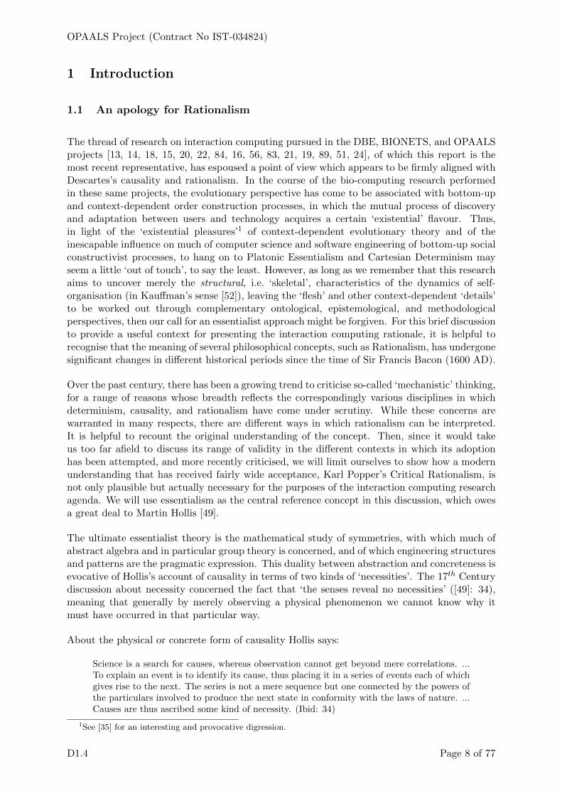
The thread of research on interaction computing pursued in the DBE, BIONETS, and OPAALSprojects [13, 14, 18, 15, 20, 22, 84, 16, 56, 83, 21, 19, 89, 51, 24], of which this report is themost recent representative, has espoused a point of view which appears to be firmly aligned withDescartes’s causality and rationalism. In the course of the bio-computing research performedin these same projects, the evolutionary perspective has come to be associated with bottom-upand context-dependent order construction processes, in which the mutual process of discoveryand adaptation between users and technology acquires a certain ‘existential’ flavour. Thus,in light of the ‘existential pleasures’1 of context-dependent evolutionary theory and of theinescapable influence on much of computer science and software engineering of bottom-up socialconstructivist processes, to hang on to Platonic Essentialism and Cartesian Determinism mayseem a little ‘out of touch’, to say the least. However, as long as we remember that this researchaims to uncover merely the structural, i.e. ‘skeletal’, characteristics of the dynamics of self-organisation (in Kauffman’s sense [52]), leaving the ‘flesh’ and other context-dependent ‘details’to be worked out through complementary ontological, epistemological, and methodologicalperspectives, then our call for an essentialist approach might be forgiven. For this brief discussionto provide a useful context for presenting the interaction computing rationale, it is helpful torecognise that the meaning of several philosophical concepts, such as Rationalism, has undergonesignificant changes in different historical periods since the time of Sir Francis Bacon (1600 AD).
Over the past century, there has been a growing trend to criticise so-called ‘mechanistic’ thinking,for a range of reasons whose breadth reflects the correspondingly various disciplines in whichdeterminism, causality, and rationalism have come under scrutiny. While these concerns arewarranted in many respects, there are different ways in which rationalism can be interpreted.It is helpful to recount the original understanding of the concept. Then, since it would takeus too far afield to discuss its range of validity in the different contexts in which its adoptionhas been attempted, and more recently criticised, we will limit ourselves to show how a modernunderstanding that has received fairly wide acceptance, Karl Popper’s Critical Rationalism, isnot only plausible but actually necessary for the purposes of the interaction computing researchagenda. We will use essentialism as the central reference concept in this discussion, which owesa great deal to Martin Hollis [49].
The ultimate essentialist theory is the mathematical study of symmetries, with which much ofabstract algebra and in particular group theory is concerned, and of which engineering structuresand patterns are the pragmatic expression. This duality between abstraction and concreteness isevocative of Hollis’s account of causality in terms of two kinds of ‘necessities’. The 17th Centurydiscussion about necessity concerned the fact that ‘the senses reveal no necessities’ ([49]: 34),meaning that generally by merely observing a physical phenomenon we cannot know why itmust have occurred in that particular way.
About the physical or concrete form of causality Hollis says:
Science is a search for causes, whereas observation cannot get beyond mere correlations. ...To explain an event is to identify its cause, thus placing it in a series of events each of whichgives rise to the next. The series is not a mere sequence but one connected by the powers ofthe particulars involved to produce the next state in conformity with the laws of nature. ...Causes are thus ascribed some kind of necessity. (Ibid: 34)
1See [35] for an interesting and provocative digression.
D1.4 Page 8 of 77

OPAALS Project (Contract No IST-034824)
Corresponding to the mathematical or abstract form of causality,
Seventeenth-century rationalists ... were deeply impressed by the luminous qualities ofmathematics, which they regarded as a model for scientific knowledge ... Mathematical truthshave the interesting feature that they not only are true but could not possibly be false. ...Facts about numbers are objective and necessary facts of a universe which, at least in theseways, could not be otherwise. (Ibid: 35) [Emphasis in original]
Cartesian determinism has been rightly criticised for ascribing the qualities of the latter to thebehaviour of the former. This is like saying that nature behaves in a particular way because theunderlying (or, better, overarching) mathematics tells it so. According to Hollis, this conflationthat seventeenth-century rationalists made of physical necessities with mathematical necessitieswas a mistake. Our view is that if, instead, we regard the mathematics as merely being concernedwith developing models of physical behaviour that have a limited range of validity, then we leavenature the initiative and ascribe to mathematics merely the ability to describe a part of whatnature does. This is the view that we follow in this report.
What is now called Cartesian determinism was one of the two possible ways in which Baconunderstood the relationship between physical and mathematical necessities: the other waywas from observables to general theories, which has given rise to Empiricism, the inductivemethod, and Positive Science. Whereas Bacon saw both progressions as ‘rational’, nowadaysPositive Science is mainly associated with quantitative statistical methods for finding correlationsbetween observables. Today, this is regarded as more descriptive than explanatory, meaning thatstatistical correlations and probabilities are not generally considered sufficient to explain causalrelationships as hidden explanations of observed behaviour. As a consequence, Bacon’s first wayis now associated with rationalism, whereas his second way is associated with empiricism, andthe two are seen as theoretically incompatible opposites. Figure 1 shows a diagrammatic viewof these concepts. Although the Divine Watchmaker is a concept that comes from the early 19th
Century, we added it to this figure since its presence and role remained very much the sameduring the previous several centuries.
Physical cause
Observable effect
Axiom
Theorem
Physical cause
Observable effect
Axiom
Theorem
Today: Cartesian Determinism,Rationalism, Causality,Deductive method
Today: Positive Science,Empiricism,Inductive method
Sense data(Objective reality)
Sense data(Objective reality)
DivineWatchmaker
Creation implies existence of Creator
Platonic Essence
'Mechanistic'Design
General Theory
"Gradual and unbroken ascent"
"Discovery of middle axioms"
Figure 1: Baconian Rationalism
Although determinism goes too far in claiming that mathematical causality entails physicalcausality, of course logical deduction in mathematics can uncover relationships between parts of
D1.4 Page 9 of 77

OPAALS Project (Contract No IST-034824)
a model that we may not have observed or even imagined between their physical counterparts.Therefore, mathematics can, and routinely does, uncover and ‘explain’ the unobservable. Butno ‘rational’ modern scientist would dare believe any such predictions without some form ofexperimental verification (or absence of falsification [79]). This suggests that the meaning ofrationalism has changed over time, and is now somewhat different to how it was understood byBacon four centuries ago. Although a discussion of Kant would be appropriate at this point ofour historical recap, since he proposed the first major synthesis of rationalism and empiricism,we fast-forward to modern times because in this report our discussion of certain aspects of thephilosophy of science is meant to be merely in support of the very specific objective of developinga mathematical theory of Interaction Computing, and Popper’s views will suffice.
As discussed more fully in deliverable D12.10 [17], Karl Popper has provided a ‘rationalisation’that reflects well both modern scientific practice and the work performed in DE research,regardless of the discipline [79]. The Popperian framework could be seen as a workableintegration of the deterministic, top-down, and deductive epistemology of rationalism with thepositivist, bottom-up, and inductive epistemology of empiricism into a circular and never-endingiterative process of progressive refinement of models, as shown in Figure 2.
System ofaxioms 1
Theorems
System ofaxioms 2
Theorems
System ofaxioms 3
Theorems
Physical cause
Observable effect
Inspires
Inspires
Inspires
Verify / Falsify
Verify / Falsify
Verify / Falsify
System ofaxioms 4
Sense data,Experimental data(Objective Reality)
Progressive Model Refinement
Figure 2: Popperian (Critical) Rationalism
Thus, the progressive model refinement espoused by Popper’s rationalism is necessary becauseinteraction computing attempts to replicate isomorphically the causal mechanisms underpinningorder construction in cell metabolic and regulatory processes, in addition to relying on biologicalconcepts as metaphors for new architectures and design patterns. This means that we wish tomap the dynamical and structural properties of cellular processes to the dynamical and structuralproperties of computational processes. In particular, we wish to replicate in software the abilityof the overall system to retain stability and robustness in spite of its openness to new componentsthat enter its periphery, triggering a wide range of possible and unexpected interactions withits existing components. Since we are trying to approximate the behaviour of unimaginablycomplex processes and systems, we could not possibly hope to succeed in one go. Therefore, wemust try to approximate the system whose properties we wish to emulate at some appropriatelycoarse initial level of abstraction, and improve our model gradually, as we understand moreabout the system and/or as we discover the fallacies of our initial approximations. The role ofsymmetry at the root of system stability to balance evolutionary open-endedness has alreadybeen discussed ([15]: 10; [17]) so we won’t repeat the argument here.
D1.4 Page 10 of 77

OPAALS Project (Contract No IST-034824)
1.2 Models in the natural/physical sciences and in computer science
A mention of models in a discussion of natural/physical and computer science could cause someconfusion, because the concept of ‘model’ is treated differently in these two disciplinary domains.The most visible difference is that whereas mathematical models tend to be analytical, computerscience models tend to be synthetic, as we now explain.
The models we have been discussing above are mathematical ‘objects’ that behave in some senseanalogously, or even isomorphically at a given abstraction level, to a suitably chosen biologicalsystem (e.g. [89]). Examples of such models are systems of differential equations derived from thebiochemical rate equations of a given metabolic or regulatory pathway [15, 16, 51]. Although theconstruction of such models is a creative and synthetic mathematical activity, they are meantto reproduce and help explain the behaviour of physical observables. Thus, their function isanalytical.
It is interesting to note that during the course of the OPAALS project we have alreadyexperienced at least one iteration in the Popperian model refinement process. In fact, ithas become apparent that the Lie group analysis of systems of non-linearly coupled ordinarydifferential equations (ODEs) modelling a given regulatory pathway such as the p53-mdm2system [51] is probably too difficult and its applicatibility too limited for it to achieve usefulpredictions in a reasonable time (< 5 years). In addition, the ODE approach does not seem tobe sufficiently granular, something we had already observed in previous reports (e.g. see [14]:16). At the practical level of obtaining usable insights within a time-frame of a year or two,therefore, the Lie group approach has for the moment been ‘falsified’, prompting us to lookelsewhere.
We had already begun to look at discrete models in three areas: symbolic dynamics wasmentioned briefly ([14]: 16); network coding has been looked at in some detail in the BIONETSproject [1]; and we began a study of abstract algebra in order to build a foundation ofunderstanding to tackle algebraic automata theory [14, 15, 22, 16, 1]. Shifting our perspectivefrom continuous to discrete models and extending the concept of model to encompass thesemantics of both mathematical and computer science models will gain us several advantages:
• A clearer way to reconcile the different epistemological viewpoints, if not quite a single epistemology
• Further iterations in the Popperian model refinement process
• A mathematical object that can benefit from the synthetic or constructive activity of softwareengineering whilst remaining compatible with the analytical nature of mathematical models ofbiological behaviour – which we believe embody the constraints required to transfer biologicalbehaviour to software.
1.2.1 Semantics
In the natural and physical sciences models, and in particular mathematical models, are able toreproduce the behaviour of observable variables because – to a suitable level of accuracy – theyembody the relationships between them and the visible and invisible causes of their behaviour.For this reason they tend to be regarded as explanatory: the model provides a verifiable causallink between the observable effect and the invisible cause.2 In software engineering, by contrast,
2For example, the velocity of a particle under the action of gravity can be derived from the mathematical‘model’ F = ma, where F is indeed invisible.
D1.4 Page 11 of 77

OPAALS Project (Contract No IST-034824)
‘domain models’ are descriptions of concepts relevant to a particular application domain and ofthe relationships between them. From these descriptions suitable data structures are derived,in support of functional code writing. Similarly, domain models can also serve as the basis forcomputational ontologies. Because such domain models account for all the causes and all theeffects in a visible way, they tend to be called descriptive rather than explanatory.
However, if we include among the objects being described explicitly also the causes of observedbehaviour, then also a mathematical model could be dubbed descriptive. In other words, amodel that is explanatory at a certain level in a causal hierarchy could be considered descriptiveat a higher level in that hierarchy. It could be argued, therefore, that mathematical modelsand domain models are not necessarily too dissimilar. Both are in essence descriptions ofobjects combined with the semantics of the relationships between them. Whereas the semanticsof mathematical models are algebraic or calculus rules that reflect physical relationships, thesemantics of domain models tend to be textual descriptions which obey specific grammar orsyntax rules and reflect given functional and non-functional requirements. Both are formalsystems and both can be made sufficiently self-consistent to allow, in the latter case, at leastsome level of ’reasoning’.
Therefore, the calculation of the consequences of mathematical models, such as the numericalevaluation of a system of differential equations to obtain the time variation of the concentrationof a biochemical compound, are not too dissimilar to the deduction of logical consequences froma semantic network or ontology using the relationships explicitly labelled as links between itsconcepts. As formal systems go, mathematical formalisms tend to be better suited to modelphenomena that ultimately arise from physical laws, possibly because with such models we havebeen trying to emulate physical behaviour for a long time, and the models had many chances tobe falsified and subsequently further improved. The same mathematical formalisms, by contrast,are rather ineffective for describing and modelling software engineering artefacts. Domain modelsor other logic-based specification languages are much better suited. This perspective will befurther explored in follow-up work inspired by [6].
1.2.2 Open model building
When computer science models need to embody biological behaviour, as in the case of bio-computing, clearly we need a new synthesis of these two perspectives. Thus, another importantaspect of models is that, even if we were not aware of Popper’s theories, the current state ofthe art in both mathematical and domain models can’t help but be regarded as still primitiveif we consider the expressiveness necessary to capture biological behaviour. We are thereforeapproaching the task of model building in each disciplinary domain, and the translations betweenthem, with an open and critical mind: we should be ready to use ideas that have proven usefulbut without being fettered by a priori epistemological assumptions.
1.2.3 Structure
Although it appears to be in principle possible to place the semantics of the models representingbiological and software systems on the same level, our claim is that it is not sufficient to do soif the objective is to arrive at software that behaves in a ‘biological’ way: we must take intoaccount also the formal structure of the models. By ‘formal structure’ we mean the presence ofa specific kind of structure, namely a hierarchy of nested formal structures charecterised by thefact that possibly different semantic rules apply at each level.
D1.4 Page 12 of 77

OPAALS Project (Contract No IST-034824)
Structural hierarchies are important for several reasons:
• When hierarchical models are developed over time, their development usually starts with identifyingthe coarse skeleton mentioned above and thereafter tends to be consistent with the Popperianframework of progressive refinement.
• When increasing refinement corresponds to increasing specificity, model hierarchies can supportmultiple epistemological positions, i.e. the ‘essentialist’/structuralist stability and generality oflarger-scale structure along with the ‘existentialist’/evolutionary context dependence of finerstructure.
• They are implicitly present in most mathematical models, although not always visible, andhave been researched for their cognitive function under the concept of ‘coordinatisation’:coordinatisation helps us understand complex problems [76, 77, 30, 81].
• They arise in software engineering artefacts simply as a consequence of architectural conceptuali-sation, requirements definition, and engineering design choices and optimisation.
• They are ubiquitous in biological systems.
We should clarify that in this discussion the term ‘structure’ is overloaded: it can carry therelatively more concrete meaning of the physical structure of biological systems and the structureof data or programs, but it can also refer to more abstract computational structures such asthe algebraic structure of the transformation semigroups that formalise automata and similarcomputational abstractions.
At different scales biological systems are governed by different physical processes, which aremodelled by correspondingly different mathematical models. Similarly, complex softwareapplications can combine efficient device drivers written directly in Assembly at the lowestlevel, with objects or similar data structures at some intermediate computational level, withdistributed online environments supporting multiple remote user interactions at the highestweb execution level. Thus, structural hierarchies usually imply also functional hierarchies andhierarchies of models. As a consequence, in spite of the vast difference between biological andsoftware systems the presence of some kind of structural hierarchy appears to be common toboth.
1.2.4 Krohn-Rhodes theory
A theory that appears to be sufficiently general to support all of the above properties(semantics, openness of models, structure) is the Krohn-Rhodes theory for the decompositionof transformation semigroups [53],3 which is why it has become the focus of attention of ourresearch in interaction computing [15]. Confronted with the possibility that biological behaviourmight only be possible if a stable set of elementary components, however many and howevercomplex, is combined with a stable set of physical laws, we postulated that correspondinglyuniversal structure laws might be needed to achieve self-organising behaviour in software. Toachieve sufficient generality the manner in which we formalise structure must be abstract enoughto be implementable in any applied context, and at potentially different scales. Further, it mustnaturally embody the dynamical properties of the systems it formalises ([21]: 114). This ishow we have arrived at the conjecture that we are dealing with a structure imposed on a statespace by a semigroup of state transformations and that therefore the appropriate object ofstudy is the finite-state automaton. As explained in previous work [21, 24, 81], then, interactingfinite-state automata appear to have the potential to model natural self-organising behaviour
3A transformation semigroup is a set of states together with a semigroup of transformations acting on it. Thus,it is the mathematical structure underpinning finite-state automata.
D1.4 Page 13 of 77

OPAALS Project (Contract No IST-034824)
by formalising for software systems a suitable set of constraints derived from natural systems,and Krohn-Rhodes theory appears to provide a very interesting first step in this direction.
In [24] we discuss how transformation semigroups can be seen as constructive dynamical spaces,where algorithms are built by concatenating semigroup elements. This is in principle sufficientlyexpressive to account for program semantics; however, how a transformation semigroup canmodel the properties of the original dynamical system is still unclear. The open character ofthe modelling effort is not so much reflected by recourse to a finite-state automaton, whoseexpressiveness is limited relative to e.g. a Turing machine, but by the fact that the automataare allowed to interact [24, 81].
We hope eventually to develop testable hypotheses for the above claims. For the present, itseems that theorem proving is the more accessible verification method. For example, we willeventually want to prove whether or not mathematical models such as systems of ODEs canactually embody features and constraints that support self-organising behaviour. Or we willwant to show that specific and recognisable algebraic structures are necessary and sufficient toformalise the constraints that support self-organising behaviour of suitably discretised metabolicsystems. Or we will want to show that it is possible to translate such algebraic structures intospecific kinds of algorithms and data structures. The concept of self-organisation, which we havecurrently described only conceptually as arising from the functional overloading of interactingfinite-state automata, will need to be defined and expressed in a suitable formal system. The‘test’ will then consist of building software environments in which software self-organisation asdefined will result as a consequence of specific architectural specifications and dynamic qualities(i.e. algorithmic characteristics satisfying non-functional requirements). So far we have onlybeen able to show that finite-state automata derived from cellular pathways do indeed haveinteresting algebraic properties. Chapter 4 of this report is therefore concerned with discussingthe possible interpretations for this algebraic structure and with presenting the latest insights inthe analysis, modelling, and emulation of biochemical systems and in particular of their orderedbehaviour.
A rationale for discretising cellular pathways, usually going through a Petri net to obtain afinite-state automaton representation, has already been presented ([15]: 13; [21]: 114-115; [24]).Our recent and current research [77, 30, 26, 29, 32] shows several examples of cell regulatory andmetabolic pathways to be formalisable as finite-state automata in this manner. The applicationof Krohn-Rhodes decomposition to the corresponding semigroups then reveals the presence ofa rich algebraic structure in the form of permutation groups and non-invertible components(so-called flip-flops) at different levels of their hierarchical decomposition.
However, as we pointed out already ([15]: 15), the algebraic structure of automata doesnot account for their time-dependent or dynamical behaviour but, rather, for the space ofcomputational trajectories they can carry out. In other words, although it accounts for allpossible dynamical behaviours, in the sense of what the automata could possibly do, it doesnot provide timing information according to an external clocktime nor any information aboutrelative likelihood of any of these trajectories.
As we discuss in Chapter 4, the holonomy decomposition of transformation semigroups yieldsgroupings of automata states arranged in a hierarchy of nested sets of states, along withthe transformations (elements of the semigroups) that operate on these sets of states.4 Thealgebraic construction that formalises this idea is called the ‘wreath product’ (or a suitable
4‘Natural subsystems’ and ‘pools of reversibilty’ (i.e. embedded permutation groups) are also identified by thedecomposition, as will be discussed in Chapter 4.
D1.4 Page 14 of 77

OPAALS Project (Contract No IST-034824)
substructure5 thereof). This kind of structural analysis, however, does not tell us anythingabout the algorithms that might exhibit interesting or useful behaviour, and it does not tellhow or why any such algorithms might be benefiting from the algebraic structure. Clearly oncethe holonomy decomposition is known many such algorithms can be derived or inferred, butthey are not a systematic output of a Krohn-Rhodes style of analysis. This is why we felt weneeded to complement the algebraic analysis of automata structure with an algebraic analysisof possible input strings, i.e. of the corresponding languages. This is addressed by the field ofSymbolic Dynamics. This point needs to be explained carefully.
Applying ‘forward engineering’ to the automaton does give us all the possible input strings (whichneed not be restricted to inputs but could include internal events – not just ‘inputs’ – dependingon the modelling). Automata constrain the possible dynamical trajectories. Formal languagetheory is very closely connected with automata and this relationship is very well studied,e.g. given a finite automaton one can give a regular expression for all the compatible inputsequences, and conversely. So studying languages associated to automata is not a particularlygood justification to move to the study of symbolic dynamics. But the timing information orlikelihood of trajectories might be inferrable by symbolic dynamics methods. Another argumentfor symbolic dynamics may be as a source of languages and automata coming from dynamicalsystems to which we can apply algebraic analysis.
For example, given a particular family of dynamical behaviours, symbolic dynamics helps usdetermine whether this family defines a shift space (dynamical trajectory in phase space =point in the shift space). Once we do that, we may be able to infer the algebraic properties ofsuch a shift space, and hence of the original dynamics. Such properties would then, hopefully,be transferrable to automata structure characteristics. This is true if the shift space is a soficshift, for example. So the motivation to build up expertise in symbolic dynamics is the followingpossible scenario: we apply it to the analysis of complicated, non-linear dynamical systemsthat exhibit self-organising behaviour; if we are able to cast such a problem as two or moreinteracting systems, this ought to correspond to two or more shift spaces that are somehow‘communicating’; once we translate them into automata, we would have a way to derive a setof interacting automata along with all their structural characteristics. As we will discuss in theConclusion, all this ought to be relatable to category theory adjunctions, although this is onlyspeculation at this point. It is for these reasons that we feel symbolic dynamics deserves anin-depth look.
1.2.5 Symbolic dynamics
Symbolic dynamics originated in the work of Hadamard in discretising geodesic flows on surfacesof constant negative curvature [44]. A geodesic flow is nothing more than a generalisation tonon-Eucledian spaces of the uniform (linear and constant) motion described by Newton’s FirstLaw in the absence of any forces on a particle or system. Symbolic dynamics grew as a tool foranalysing general dynamical systems by discretising space [97], and it can therefore be seen asa complement to the Poincare map, which transforms a continuous flow into a discrete iteratedmap by discretising time. As discussed by Morse and Hedlund,
The methods used in the study of recurrence and transitivity frequently combine classicaldifferential analysis with a more abstract symbolic analysis. This involves a characterizationof the ordinary dynamical trajectory by an unending sequence of symbols termed a symbolic
5‘Substructure’ is better than ‘subset’ here because it is actually a sub-transformation semigroup.
D1.4 Page 15 of 77

OPAALS Project (Contract No IST-034824)
trajectory such that the properties of recurrence and transitivity of the dynamical trajectoryare reflected in analogous properties of its symbolic trajectory. [73]
Recurrence is the tendency of a dynamical system’s trajectory to revisit a particular pointor region of phase space, whereas transitivity is concerned with the ergodic properties of thetrajectory, i.e. its tendency to come arbitrarily close to any point in a given phase space volume(generally defined by the system’s energy).
Thus, from the beginning, symbolic dynamics was concerned with some aspects of the globaland long-time properties of dynamical systems, expressed through an algebraic rather than acalculus formalism. As we will see in Chapter 2, this kind of analysis tells us which trajectoriesare admissible and which are not, where each trajectory is expressed as a doubly-infinite sequenceof symbols from a given alphabet. Since we can define a special kind of space called a ‘shiftspace’ whose ‘points’ are these sequences, we can think of these infinite sequences of symbols asanalogous to the infinite decimal expansion of a real number ([62]: xi). We can see, therefore,that symbolic dynamics works with mathematical objects that are compatible with continuousdynamical systems, but that are in fact composed of discrete entities. For this reason this theoryseemed relevant to the bio-computing research agenda.
There are two more reasons that in our view justify investing in this area of research. First, oneof the main areas of application of symbolic dynamics is network coding, which we have studiedin the BIONETS project [20]. In particular, trellis codes [80] appear to be potentially relevantto the architecture of interacting automata. Second, as we will see in Chapter 2 certain kindsof shift spaces can be related directly to regular languages and finite-state automata.
Having provided a philosophical and mathematical overview underpinning interaction computingresearch, we now continue the development of the concepts related to interaction computing, withthe understanding that this conceptual framework is only a stepping stone towards a suitablemathematical formalisation.
1.3 Interaction computing and its derivatives
We start by reproducing Figure 3 from D1.3 [15]. Whereas symbiotic computing is relevantto e.g. the concept of symbiotic security [83] and autopoietic computing is discussed in thecompanion deliverable D1.5 [7], this report is more concerned with gene expression computing.
Interaction Computing
Gene ExpressionComputing
SymbioticComputing
Autopoiesis-InspiredComputing
Figure 3: Interaction computing and its derivatives
1.3.1 Gene expression computing
Gene expression computing refers to the ability to specify environments that, in turn, cangenerate software services in response to internal or external stimuli. Thus, gene expression
D1.4 Page 16 of 77

OPAALS Project (Contract No IST-034824)
computing aims to reproduce the ability of the biological cell to synthesise particular functionalcomponents such as enzymes in response to the needs of on-going metabolic processes or tosignal transduction pathways from outside the cell. The signals to initiate the synthesis ofsuch components are somehow ‘encoded’ in the metabolic processes themselves, i.e. in priorbiochemical reaction products. If the purpose of these reaction products is to trigger thesynthesis of the enzymes, then the causal chain is linear and relatively straightforward. If,instead, the reaction products are needed for some other purpose and, at the same time, theyencode the trigger for the expression of the enzyme(s), then we have a case of functionaloverloading that is the root of the concept of symbiotic computing.
In any case, services generated in this manner should be considered ‘atomic’ in some suitablesense and many of them need to be composed dynamically to produce the complex behaviour thatwe associate with a software service of average size and complexity. The dynamic compositionprocess is similar in character to the sequences of biochemical reactions that make up metabolicand regulatory pathways.
The above description glosses over an important point which we have not addressed properlyin previous work and that we wish to rectify here. Since the first deliverable on bio-computingin the DBE project [13] we have acknowledged that software systems are devoid of interactionpotential energy between their components as well as of a property analogous to temperature.The argument we have been making since then is that these two properties of physical andbiochemical systems, upon which processes like the minimisation of free energy depend, arereplaced in our vision of self-organising software ecosystems by user inputs that are propagatedthroughout the digital environment through a series of cascaded state transitions, similar toa domino effect. However, upon further scrutiny this does not now look realistic because,similarly to a biological system, the number of such external triggers is much much smaller thanthe number of internal components of the system and especially of the possible system states.Thus, it now seems more plausible to claim that the external triggers act like signals rather thanas actuators of thermodynamic mixing.
The need to re-introduce an analogue to temperature is daunting but may not be such a foreignconcept to software systems after all. From a statistical point of view, the effect of temperaturein physical systems is to locate the system’s internal dynamics at some point between totalorder (frozen structure of a crystalline solid) and total chaos (totally random and ever-varyingstructure of a gas). In a biological system, the energy implicit in a temperature value thatfalls in the lower half of the liquid phase of water is harnessed to drive a huge number ofautomatic functions that are nested and distributed at many scales. The signals that comefrom the ‘outside’ (a term whose precise meaning depends on the definition of ‘system’ beingemployed in any one instance) can only modulate the large number of operations that are alreadytaking place. This execution architecture corresponds to a large number of ‘Do Forever’ loopsthat are interlocked and that keep a whole system running in some kind of ‘idle’ mode, like alarge and dumb machine. This is where most of the ‘energy’ is. Low-energy external signalsthen behave like the base current in a transistor, they carry the critical information that cansway the large ‘machine’ in different directions. The functional overloading may then refer tothe nesting, interdependence, and scalewise overloading of such control signals, a view that isstrongly reminiscent of the cybernetics vision, and in particular of Ross Ashby’s Law of RequisiteVariety [2].
To postulate a huge number of idle loops cycling through a fixed number of states, at differentscales, is not so unreasonable if we compare this picture to the properties of large digitalsystems. In the internet, for example, servers, switches, and routers are constantly performingan astronomical number of repetitive operations that at the lowest syntactical level are rather
D1.4 Page 17 of 77

OPAALS Project (Contract No IST-034824)
meaningless but that are nonetheless compiled from higher-level instructions. The differencebetween the internet today and a biological system is that in the former the number of internaloperations is of a similar order of magnitude as the number of external stimuli, whereas in thelatter this is not the case. The number of internal operations is astronomically larger than thenumber of external stimuli.
What allows us to make this claim for biological systems is that we are neglecting molecularinteractions below the threshold of the simplest organic molecules. This allows us to separateexternal stimuli in a similar way: for example, we can neglect the collision of air molecules withthe skin, but consider smells as valid signals. In the case of the internet, we are separatingthe internet itself from the applications that may be running on servers and which obviouslycontain a huge number of operations. What makes this possible is the engineering practice ofmodularisation and layering, which separates different aspects of the overall systems. In biology,on the other hand, subsystems cannot afford to be independent because there would be nothingtransmitting the information between them that underpins their cooperation or, perhaps better,choreography. In other words, in biology every subsystem is tightly coupled if not to everythingelse at least to its adjacent subsystems, whereas in software engineering we have been strivingto work towards loose coupling as much as possible.
Thus, a necessary architectural requirement for self-organising systems built on gene expressioncomputing appears to be to base high-level functions on a nested hierarchy of basic and repetitivefunctions that can be increasingly automated as one moves down the hierarchy towards smallerscales of system description and ever-greater numbers of components.
1.3.2 Symbiotic computing
At an applied level symbiotic computing can be explained through the example of symbioticsecurity. As discussed in Schreckling et al. ([83]: 36), symbiotic security captures the balancebetween the encapsulation of a security function in a specialised security service with theinterdependence between such a service and the service(s) it is meant to secure. In other words,in order to address the problem posed by the ‘ex post patching paradigm’ in the development ofsecurity services and applications,6 we felt it would be worth investigating a mode of generationof such paired services based on the integration of their most fundamental functions ex ante.This is similar to how the human immune system is inextricably integrated with the nervousand endocrine systems [11].
As a consequence, in symbiotic security a security service is assumed to be tightly coupled tothe services it is meant to secure. Thus, neither can be executed by itself, both need the otherservice to do anything. Each service is functionally overloaded to perform its function and totrigger state transitions in the service it is coupled to. Since the concept of service appliesat different scales, gene expression computing becomes a general framework that can supportthe more specific symbiotic computing, whose realisation requires the enforcement of additionalsuitable constraints.
6The ex post patching paradigm does not develop new security services or applications but, rather, patchesthe corresponding applications after realising that they have a problem.
D1.4 Page 18 of 77

OPAALS Project (Contract No IST-034824)
1.3.3 Autopoietic computing
Autopoietic computing [7], finally, is concerned with adding recursion as a fundamental propertyof every element of the architecture. Thus, similarly to how we can say in a service-orientedarchitecture that ‘everything is a service’, so in autopoietic computing we can say that‘everything is an autopoietic service’. This means that every element of the architecture, atevery scale, is overloaded, as follows:
• The primary function is defined by functional specifications as in any architecture.
• The secondary function that the primary function also contributes to is to support the replicationof a strategically defined architectural unit, which is analogous to the biological cell.
It is not unreasonable to postulate that the manner in which the autopoietic function is realisedmay depend on applying recursion to symbiotic computing. In other words, a framework thatcould integrate all three types of computing might be to overload three or even more functionson cellular components:
• The primary function is defined by functional specifications as in any architecture.
• The secondary function that the primary function also contributes to is to support other metabolicpathways, for instance by triggering the expression of suitable enzymes.
• (Other intermediate and probably scale-dependent functional levels are possible)
• The highest-level function that the primary, secondary, etc functions also contribute to is ultimatelyto support the replication of a strategically defined architectural unit, which is analogous to thebiological cell.
The hypothesis is that as we go from a single component to the whole cell (or its analogue insoftware) the different levels of functional overloading are coupled by binary symbiotic computingrelationships.
The principle by which the highest-level function of multiple components is organised is called‘operational closure’ and has been discussed in [14, 18, 15], as well as in [7] and in theoriginal sources [65, 66]. The motivation for attempting to achieve the highest-level, replicativefunction is to increase the morphogenetic and adaptation properties of software applicationsand services through a continual renewal of its core components. The continual renewal oflower-level components could be one type of the ‘Do Forever’ loops that are necessary to holdthe system in a dynamic state that can transition quickly to different ‘macrostates’ dependingon the inputs it receives, as we discussed above. In other words, autopoietic computing isimportant for extending the self-organisation ability of single atomic services to greater scales,ultimately aiming for veritable autonomous ‘digital organisms’. The difference is already well-established in computer science as the difference between a module containing some functionalcode and a module containing some functional code and an internal representation of itself andits environment – i.e. an agent. Surprisingly, to integrate the various types and levels of bio-computing it appears that such agents will need to be tightly rather than loosely coupled, whichgoes against current trends in the architecture of distributed software systems.
1.3.4 Integrating the different types of bio-computing
Once the interactions inside the cell, between cells, and between aggregates of cells have beentranslated into computer science rules subject to suitable algebraic constraints, we will be ready
D1.4 Page 19 of 77

OPAALS Project (Contract No IST-034824)
to build an evolutionary framework around the whole construction and will finally be able to‘launch’ a software ecosystem and watch it evolve over time. Figure 4 (based on a similar figurein [21]: 119) shows the relative importance of different modelling perspectives at different scales.Although the time axis is technically a 3rd dimension, in this 2D diagram it is drawn parallel tothe length scale axis; a 3D diagram would have been too difficult to draw and not very clear.
Biology "floor"
Physics
LengthScale
Order from Interactions: Algebra, Dynamical Systems
Order from History & Memory:
Learning, Evolution, Adaptation
Localtimeaxis
Multi-cellular
organisms,up to
ecosystems
Single cellsand uni-cellular
organisms
Sub-cellularsystems
Structuralcoupling
OperationalClosure &Autopoiesis
Autopoieticcomputing
Geneexpressioncomputing
Symbioticcomputing
Biochemistry
Evolutionarycomputing
Figure 4: Schematic showing the different relative importance of order constructionmechanisms in biology, at different scales of description, and the corresponding relevance ofdifferent kinds of bio-computing. Green background indicates memory/history-dependentprocesses developing over time, yellow background indicates instantaneous dynamicalinteractions and reliance on a scale-invariant mathematical model of interaction computing.
The argument so far sounds good, but unfortunately it rests on a clay foundation. Nothingof what has been described will be possible without resolving a root problem, which we seeas a mathematical problem in its essence: we need to understand and formalise the (probablyrecursive and scale-invariant) mathematical nature of interaction computing. All our work todate suggests that this is a very difficult mathematical problem, but that, if solved, it has thepotential to revolutionise how we think about computing and how we go about designing andimplementing software.
In this final report on interaction computing in the OPAALS project we have not solved thismathematical problem. However, we feel we have made significant conceptual, theoretical, andmathematical advances. In Chapter 2 we give an introduction to symbolic dynamics to providea basis for further work and exploration. In Chapter 3 we give an update on recent experimentalfindings in the p53-mdm2 system. In Chapter 4 we provide an update on our results in algebraicautomata theory. Finally, in Chapter 5 we sum up the last 8 years of insights into a few highlightsand draw some conclusions that will set the stage for our next steps in this line of research.
D1.4 Page 20 of 77

OPAALS Project (Contract No IST-034824)
2 Symbolic Dynamics
In this chapter we need to introduce the basic concepts of symbolic dynamics in order to providea foundation for further work and an eventual bridge to algebraic automata theory. We beginwith a discussion of how symbolic dynamics has been applied to the long-time analysis of non-linear dynamical systems [47] in order then to show some striking similarities with the p53-mdm2ODE model we developed in previous OPAALS work [15, 89]. Where needed we also rely onWilliams’s very clear explanations [97]. The second part of this chapter focusses instead onLind and Marcus’s textbook on symbolic dynamics and coding [62]. As in all our deliverables onbio-computing in the DBE, BIONETS, and OPAALS projects (e.g. [13, 22, 16, 14]), the detaileddiscussion of textbook material is done for two main reasons:
• Our discussion usually goes in more detail than the textbook it is drawn from whilst being selectiveof the topics that are discussed. This is done to make the material more accessible to a widerinterdisciplinary audience while optimising the presentation for the objectives of the report.
• Since our research programme in bio-computing began in 2002 and is likely to continue for at leastanother 5 years, a very careful exposition is invaluable to guarantee our own ability to access andreconstruct the arguments months or years after the reports have been written.
In order to put the discussion of symbolic dynamics in context, Figure 5 shows how thistopic fits within the broader mathematical research workflow that we have been following anddocumenting in several reports in the OPAALS and BIONETS projects. We meant to look fora possible bridge between the discretisation of the p53-mdm2 system by symbolic dynamics andthe discretisation of the same system via the Petri net approach, discussed in [24] and in Chapter4 in this same report, but we ran out of time. Therefore, the second part of this chapter willinstead summarise the basics of symbolic dynamics as presented by Lind and Marcus [62] from acoding rather than a dynamical systems perspective. The motivation is that Lind and Marcus’stext is comprehensive and covers also sofic systems in detail, i.e. shift spaces that correspond tofinite-state automata. Although we did not get this far in the OPAALS project, our next stepin the development of a suitable mathematical framework for interaction computing will be toreconcile Krohn-Rhodes theory with the symbolic dynamics perspective.
Rings &fields
Networkcoding
Convolutionalcodes (LDPC codes)
Cellmetabolic/regulatorysystems
Dynamicalsystems(ODEs)
Symbolicdynamics
Soficshifts*
Regularlanguages*
Finite-stateautomata*
Algebraicautomata theory
Slidingblock codes
Tree ortrellis codes
Interactingautomata
Topics emphasisedin OPAALS D1.4
OPAALSD1.1
OPAALS D1.3,BIONETS D2.2.9
BIONETSD2.1.1
BIONETSD2.2.4
Groups
BIONETSD2.2.4,D2.2.9,D3.2.7,D4.6
(* Indicates topics that are closely related although they are not connected by an arrow in this diagram)
Dualrelationship?
Petrinets
Semigroups*
BIONETSD4.6
Figure 5: (Tentative) high-level view of the mathematical research workflow
D1.4 Page 21 of 77

OPAALS Project (Contract No IST-034824)
2.1 Symbolic dynamics from the point of view of dynamical systems
2.1.1 The logistic map
In this section we build some basic machinery that will enable us to show how symbolic dynamicscan be used to analyse some of the properties of chaotic dynamical systems. An introductionto the history of the logistic map as a deceptively simple model for population growth can befound in most introductory books on chaos theory, such as [47] itself. One of our objectives inthis chapter is to maintain the link to dynamical systems as intuitively clear as possible. This isbecause as we develop the abstract formalism of symbolic dynamics and eventually reach shiftspaces that are equivalent to finite-state automata what tends to happen is that one forgets theintuitive connection to dynamical systems and is therefore less able to apply physical intuition,for example, in interpreting abstract algebraic automata theory results (e.g. Chapter 4).
Thus, we start with the 1st-order ordinary differential equation for the logistic population growthmodel
x′ = λx(1− x), (1)
If we plot the derivative as a function of x, in the spirit of the jet space ([16]: 26; [51]), we geta graph as shown in Figure 6.7 In this figure λ is approximately equal to 4.2.
x
x'
0 1
1
Figure 6: Visualisation of the rate of change of x as a function of x
The equation we want to work with is a discrete version of this system, and can be approximatedsomewhat crudely by the so-called logistic map, shown for a similar value of λ in Figure 7:
fλ(x) = λx(1− x). (2)
Here fλ(x) is the fraction of some optimal population level at a future time-step as a functionof the current level. This is an iterated map, meaning that the result fλ(x) is fed back into thefunction as the argument x, and for any initial value of x = x0 in the unit interval I = [0, 1]this process is repeated forever. As shown in Figure 8, there is an easy graphical visualisationof the orbit. From any starting point x0 in the unit interval one draws a line to fλ(x0). Thisnow becomes the next x, say x1. If we draw a horizontal line through fλ(x0), the point whereit intercepts the diagonal y = x will necessarily be above the value x1 = fλ(x0). Thus, fromthis point we just have to move up or down until we meet the logistic curve again, which is justfλ(x1) = x2, and so forth. Figure 8a shows how all the points that start within the interval
7In [16, 51] the graph is a surface because the ODE being analysed is non-autonomous. The equation givenhere on the other hand is not a function of time, so a simple line graph is sufficient.
D1.4 Page 22 of 77
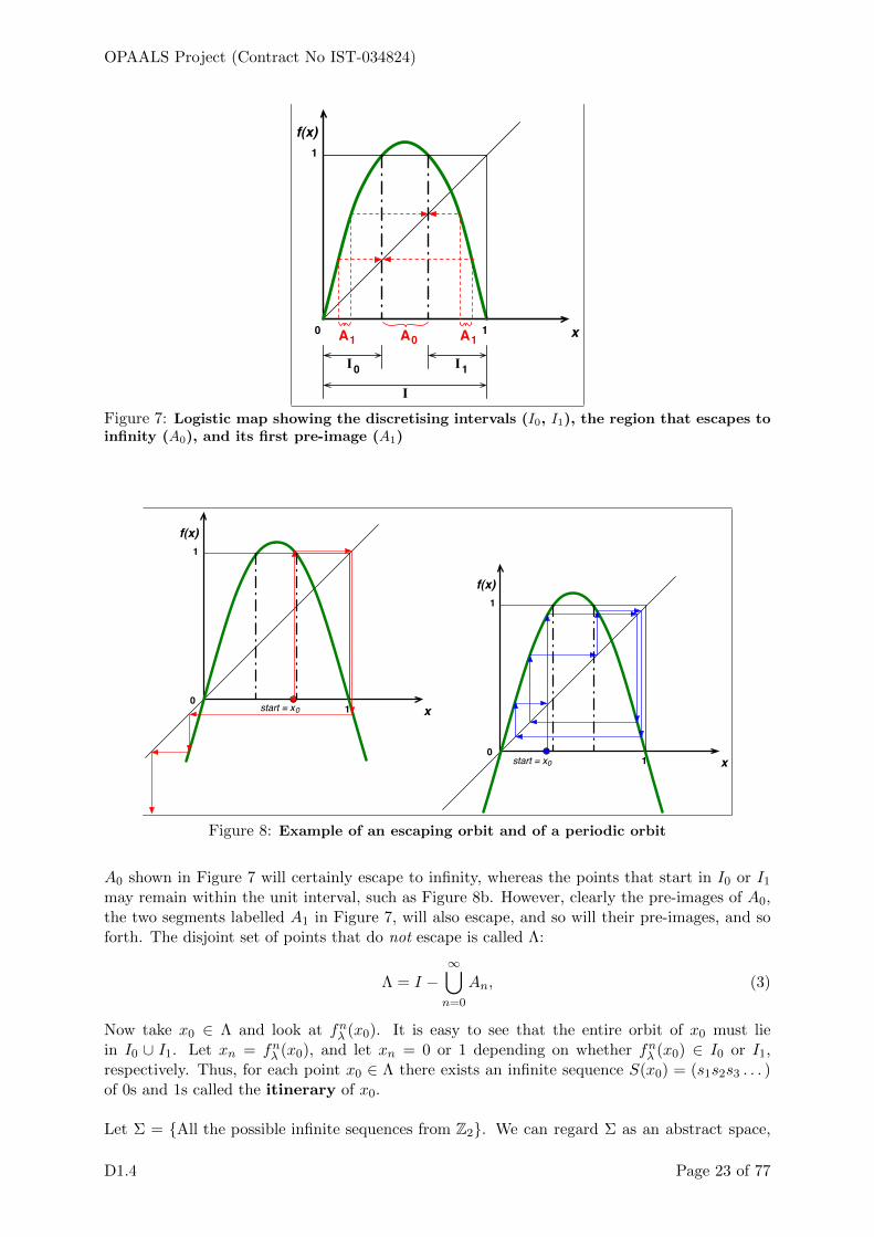
OPAALS Project (Contract No IST-034824)
A1 A10 1
1
A0I0 I1
I
x
f(x)
Figure 7: Logistic map showing the discretising intervals (I0, I1), the region that escapes toinfinity (A0), and its first pre-image (A1)
01
1
x
f(x)
start = x0
01
1
x
f(x)
start = x0
Figure 8: Example of an escaping orbit and of a periodic orbit
A0 shown in Figure 7 will certainly escape to infinity, whereas the points that start in I0 or I1may remain within the unit interval, such as Figure 8b. However, clearly the pre-images of A0,the two segments labelled A1 in Figure 7, will also escape, and so will their pre-images, and soforth. The disjoint set of points that do not escape is called Λ:
Λ = I −∞⋃n=0
An, (3)
Now take x0 ∈ Λ and look at fnλ (x0). It is easy to see that the entire orbit of x0 must liein I0 ∪ I1. Let xn = fnλ (x0), and let xn = 0 or 1 depending on whether fnλ (x0) ∈ I0 or I1,respectively. Thus, for each point x0 ∈ Λ there exists an infinite sequence S(x0) = (s1s2s3 . . . )of 0s and 1s called the itinerary of x0.
Let Σ = {All the possible infinite sequences from Z2}. We can regard Σ as an abstract space,
D1.4 Page 23 of 77

OPAALS Project (Contract No IST-034824)
and each infinite sequence as a ‘point’ in this space. We can define a distance over Σ between twopoints s = (s1s2s3 . . . ) and t = (t1t2t3 . . . ) as long as the definition satisfies the three requiredproperties of equivalence, symmetry, and triangle inequality. A function that does is:
d(s, t) =
∞∑i=0
|si − ti|2i
. (4)
Since the geometric series∑∞
i=0 xn converges to 1
1−x for x < 1,
∞∑i=0
1
2i=
∞∑i=0
(1
2
)i=
1
1− 1/2= 2. (5)
Therefore, our definition of distance also converges since the numerator for each value of i iseither 0 or 1. With this, we can show
Proposition 2.1 If two sequences s and t are equal in their first n+ 1 values, then d(s, t) ≤1/2n.
Proof.
d(s, t) =
n∑i=0
|si − ti|2i
+
∞∑i=n+1
|si − ti|2i
= 0 +|sn+1 − tn+1|
2n+1+|sn+2 − tn+2|
2n+2+ . . .
=1
2n+1
(|sn+1 − tn+1|
20+|sn+2 − tn+2|
21+ . . .
)≤ 1
2n+1
∞∑i=0
1
2i=
1
2n+12 =
1
2n(6)
We are going to state and explain but not prove the first important result of symbolic dynamics:
Theorem 2.2 The itinerary function S : Λ→ Σ is a homeomorphism for λ > 4.8
This theorem is saying that for each point x ∈ I that does not escape under the repeated actionof fλ(x) there exists one and only one sequence S(x) ∈ Σ. Therefore, by studying the propertiesof the elements of Σ, i.e. infinite sequences of symbols taken from the alphabet Z2, we willautomatically be studying the properties of the orbits of the logistic map.
Definition 2.3 The map fλ : I → I is chaotic if
• Its periodic points are dense in I, i.e. they come arbitrarily close to any point in I.
• fλ is transitive on I: for U1, U2 ⊂ I, ∃n : if x0 ∈ U1, fnλ (x0) ∈ U2.
• fλ has sensitive dependence on I: this means that the distance between any twoarbitrarily close points will diverge and will be greater than an arbitrarily chosenconstant after a sufficient number of iterations. In mathematical language, this conceptis expressed as follows: let U ⊂ I be an arbitrariry small open subset of I centred aroundx0. Then, ∃β > 0 : ∀x0 ∈ I and x0 ∈ U, ∃(y0 ∈ U, n > 0) : |fnλ (x0)− fnλ (y0)| > β.
Definition 2.4 Let I and J be two different intervals, and f : I → I, g : J → J . Then, fand g are conjugate if there exists a homeomorphism h : I → J such that h ◦ f = g ◦ h.
8A homeomorphism is a 1-1, onto, invertible, and continuous map.
D1.4 Page 24 of 77

OPAALS Project (Contract No IST-034824)
2.1.2 Number expansions in different bases
Now let’s look at another possible map, shown in Figure 9 along with a possible orbit, which isconstructed as above. This is called the doubling map, g : I → I:
g(x) = 2x mod 1, (7)
and its dynamics are particularly interesting. In fact, if the unit interval is divided into I0 and I1as shown and the symbols of the itinerary are taken from Z2, then the itinerary for any x ∈ [0, 1]is none other than its binary expansion.
01
1
x
g(x)
start = x = 0.320
I0 I1
0.32 = 0.01010001111...
Figure 9: Doubling map, showing the binary expansion of the number 0.32
The binary expansion and doubling map may look unfamiliar, but they become more accessibleif one compares them with the decimal equivalent (over the same interval), h : I → I:
h(x) = 10x mod 1, (8)
It should be fairly obvious that repeated iteration of the above map applied to a decimal realnumber in decimal notation will give that number back. Figure 10 shows a graphical visualisationof the decimal-to-binary conversion for fractional numbers, to aid the intuition.
0
0.1 0.2 0.3 0.4 0.5 0.6 0.7 0.8 0.9 1
0 10.10.01 0.11
0.001 0.011 0.101 0.111
Notationalcorrespondence
Physicalcorrespondence
Decimal
Binary
0.010.001
Figure 10: Conversion between decimal and binary fractional numbers
D1.4 Page 25 of 77

OPAALS Project (Contract No IST-034824)
It would appear from the above that the concept of discrete iterated map is quite powerful, sothat not only can it model dynamical systems like the population growth equation, but alsoconversions between different number systems. However, the converse of this statement is moreinteresting: the concept of number system appears to be so powerful that it can be generalised.In other words, the logistic map can be seen as a very radical generalisation of the concept ofnumber system: it appears that symbolic dynamics gives a way to express the behaviour of adynamical system by means of a discrete ‘model’ that in its essence is no different to a (rathersurprisingly defined) number system.
The reason for pushing this somewhat strange point is that it is beginning to look like an insightof rather general relevance. In fact, it turns out that the automata decomposition theory andresults that we will discuss in Chapter 4 can most easily be understood and conceptualisedthrough the same identical concept of generalised number system.
There is a more abstract and at the same time more intuitive way to express this concept,as ‘coordinatisation’. This has been discussed in many publications in the last 20 years inthe specific context of Krohn-Rhodes theory [76, 77, 30, 81], as we already mentioned in theIntroduction, but it can certainly be considered a concept that has pervaded the mathematicalmodelling of any and all physical phenomena for as long as mathematical modelling has existedas a cognitive process. It appears to be truly a concept of fundamental importance.
The leap between the binary expansion and the logistic map is perhaps too big to make in onestep, even at an intuitive level. It may therefore help to mention the so-called β-expansions, i.e.
expansions in a non-integer base [97, 36]. If for example we let β = 1+√5
2 = γ, the so-called‘golden mean’, the map g : I → I in this case is:
g(x) = γx mod 1, γ =1 +√
5
2, (9)
and the corresponding graph is shown in Figure 11. To help understand this diagram, note how,because of the form of both the doubling map (7) and the golden mean map (9), the point wherethe function meets g(x) = 1 is 1/base. This, therefore, is the point that divides the two intervalsI0 and I1, in both cases.
01
1
x
g(x)
I0 I1
!
"1
!
" =1+ 5
2
!
" =1+1
"
!
"1
Figure 11: Map for a non-integer β-expansion. In this case β = golden mean = γ
D1.4 Page 26 of 77

OPAALS Project (Contract No IST-034824)
It should be fairly easy to see from this graph that any trajectory that falls within I1 at any onetime-step must switch to I0 at the next time-step. However, the converse is not true, resultingin the fact that the itineraries generated by this map cannot contain the block of symbols (11).A number expressed in this base could be converted back to decimal (at least to some desiredaccuracy since γ is a non-terminating irrational number in decimal) using the familiar formulafor positional notation:
x = γndn + γn−1dn−1 + · · ·+ γ2d2 + γ1d1 + d0 + γ−1d−1 + γ−2d−2 + · · ·+ γ−md−m, (10)
where di ∈ Z2 since in beta expansions the alphabet is formed by the integers starting at zero thatfit within the base, and γ = 1.61... . Thus, the above number would be indistinguishable froma binary number, based on the notation alone, which makes it necessary to indicate explicitlywith a subscript when one is using a non-integer base: 10110001.1010γ . The decimal point isimmediately to the right of the d0 digit, and negative powers indicate fractional digits.
Before we leave the discussion of possible connections between dynamical systems and numbersystems, since the logistic map is a smooth curve (a parabola), to develop the concept ofa generalised number system we would need to look for the ‘base’ of the expansion of anyone starting point x0 ∈ [0, 1]. Using the usual calculus argument the smooth curve can beapproximated as a series of linear segments, to each of which we would assign a correspondinginterval Ii, i = 0, ..., n, and we would then let n go to infinity and the size of the intervals go tozero. This would lead to a rather strange number system with an infinity of bases (one of eachvalue of the tangent to the parabola) and an infinite alphabet, something that may not evendefinable formally.
But perhaps this is not quite necessary. In fact, for the logistic map we have already divided theunit interval into two sub-intervals, and we have already defined a convenient itinerary functionS : Λ → Σ that approximates the infinite sequence of x-values from Λ into an infinite string ofbinary digits. Williams sums it up nicely:
We see here an exchange of spatial information for time series information mediated bydynamics: We can recover the complexity of the continuum I from our crude 2-elementpartition, provided that we observe the evolution of the system for all time. [97]
So one reason for this laborious detour into number systems is that it enables us to hold twodifferent pictures in our mind at the same time and for the same physical entity:
• The time-evolution of a dynamical variable such as population level starting at value x0 and crudelydiscretised as a time series of binary levels.
• The same sequence of binary digits as an expansion of the same initial value x0 in an unknownand mysterious base, i.e. the same time series interpreted as a single number.
These two perspectives will now help us introduce two more concepts that form the bedrockof symbolic dynamics in a way that will hopefully look intuitively connected with dynamicalsystems. The two concepts are the shift map and the equivalence of the shift map to the logisticmap. ‘Equivalence’ is meant in a very specific sense that will require some unpacking, as wenow show.
D1.4 Page 27 of 77

OPAALS Project (Contract No IST-034824)
2.1.3 The shift map and its dynamical properties
Although in this report we are not going to be able to discover the mysterious base – or if iteven exists – the second perspective in the itemised list above is useful to us because it helpsus understand the shift map. In fact, if we apply the function we used to generate the binaryexpansion of a decimal number, Eq. (7), to the same binary number we generated, we will noticethat the effect will be to shift the decimal point to the right by one position or, equivalently,the whole string to the left by one position, and drop the first digit. Because we are operatingon objects that are already in Σ, we are not talking about the doubling map (7) here, but of anew map which we call σ : Σ→ Σ such that
σ(s0s1s2 . . . ) = (s1s2s3 . . . ) (11)
It turns out that this simple and seemingly innocent map is quite powerful. Recalling thatfλ : Λ→ Λ, we wish to construct σ with the following properties ([47]: 347):
• σ is chaotic
• σ on Σ is conjugate to fλ on Λ
• σ is completely understandable from a dynamical systems point of view.
Proposition 2.5 ([47]: 347) The shift map σ : Σ→ Σ is continuous.
Proof. Let s = (s0s1s2 . . . ) ∈ Σ, and let ε > 0. Choose n so that 1/2n < ε. Let δ = 1/2n+1.Suppose that d(s, t) < δ, where t = (t0t1t2 . . . ). By Proposition 2.1 his means that si = tifor the first n+ 2 symbols, i.e. i = 0, . . . , n+ 1. Now,
σ(s) = (s1s2 . . . snsn+1sn+2sn+3 . . . ) (12)
σ(t) = (s1s2 . . . snsn+1tn+2tn+3 . . . ), (13)
Meaning that the two new sequences are equal for the first n + 1 symbols. Therefore,d(σ(s), σ(t)) ≤ 1/2n < ε. Hence, σ is continuous.
We need σ to be continuous in order to be able to form a homeomorphism with λ, which isneeded to prove conjugacy:
Proposition 2.6 ([47]: 347) The itinerary function S : Λ → Σ is a conjugacy between thelogistic map fλ and the shift map σ.
Proof. Having already stated that S is a homeomorphism in Theorem 2.2, we just need toshow that S ◦ fλ = σ ◦ S. Recall that fλ : Λ → Λ and σ : Σ → Σ and let x0 ∈ Λ andS(x0) = (s0s1s2 . . . ). Then,
x0 ∈ Is0 , fλ(x0) ∈ Is1 , f2λ(x0) ∈ Is2 , . . . (14)
But then, S(fλ(x0)) = (s1s2s3 . . . ), meaning that
S(fλ(x0)) = σ(S(x0)), (15)
which is kind of trivial in hindsight.
D1.4 Page 28 of 77

OPAALS Project (Contract No IST-034824)
We have shown the following:
ΛS−−−−→ Σ
f
y yσΛ
S−−−−→ Σ
(16)
and, in particular,
x0S−−−−→ S(x0)
f
y yσx1
S−−−−→ S(x1).
(17)
Hirsch et al. [47] make the point that the shift map is much more nicely behaved than thelogistic map. Hence it is worth pushing the argument a bit more in order to show that thesetwo functions are actually equivalent. By ‘elevating’ the shift map to the level of a dynamicalsystem of equivalent complexity to fλ, we will gain the ability to draw conclusions about fλby working with σ. This of course is the original motivator for the development of the field ofsymbolic dynamics in the first place.
One area where it is easy to see that σ is easier to work with is in the classification of the periodicpoints of the map. In fact, any periodic point of length n will have the form, (s0, s1, s2, . . . , sn−1).For any value of n, therefore, there will be 2n periodic points. On the other hand, since x ∈ Rfor the logistic map, it would be horrendously difficult to find, let alone completely classify, thecorresponding periodic points for fλ. The reason we know that they exist and that there is a1-1 correspondence between the two sets of periodic points is because we have just proven inProposition 2.6 that fλ and σ are conjugate.
We now show that σ is chaotic. Following Definition 2.3 we can construct a point in Σ whoseorbit is dense as follows:
s∗ = (0 1 00 01 10 11 000 001 010 011 100 101 110 111 . . . ) (18)
Thus, s∗ contains all the strings of any length, arranged in order of increasing size. Now assumethat we want to match an arbitrary sequence t in its first n places. All we have to do is iterateσ(s∗) a sufficient number of times, say k, until we find the block in s∗ of length n that matchesthe first n symbols of t. This will ensure that
d(σk(s∗), t) ≤ 1
2n−1. (19)
By increasing n and k we can bring a future iterate of s∗ as close as we want to any given stringt. Therefore, s∗ is dense under σ in Σ, which means that σ is transitive. As Hirsch et al. [47]explain we can create any number of other points that are dense in Σ, simply by rearrangingthe blocks shown in Equation (18). To identify a point in Λ whose orbit under fλ is denseis unfathomable. This, therefore, is what we mean when we say that the dynamics of σ are‘completely understandable’.
Finally, we need to address sensitive dependence on initial conditions. Let’s choose the constantβ of Definition 2.3 as 2, since this is the largest distance possible between two points in Σ(see Equation (5)). We need to show that the distance between two points that are initiallyarbitrarily close will, after a suitable number of iterations, reach this maximum distance. To
D1.4 Page 29 of 77

OPAALS Project (Contract No IST-034824)
this end we define the symbol s as meaning ‘not s’, i.e. if s = 0, s = 1, and vice versa. Now wepick the point s′ such that
s = (s0s1s2 . . . snsn+1sn+2 . . . )
s′ = (s0s1s2 . . . snsn+1sn+2 . . . ).
We thus have, by construction, that
d(s, s′) =1
2n
d(σn+1(s), σn+1(s′)) = 2.
With the above, we have in fact proven
Theorem 2.7 ([47]: 348) The shift map σ is chaotic on Σ, and so by the conjugacy provenby Proposition 2.6 the logistic map is chaotic on Λ when λ > 4.
Taking stock of how far we have got, we have shown that symbolic dynamics provides a powerfulanalytical tool to investigate the properties of dynamical systems. However, it does not yetappear to enable us to build a dynamical system according to a specification. This is a long-term goal that we will continue to keep in mind. For the time being we will continue to buildformalisations that can act as a bridge between dynamical systems and computing systems,classifying and documenting important properties as we encounter them. In this spirit we nowspend a few words on higher-dimensional dynamical systems before switching the perspectiveto coding.
2.1.4 Homoclinic phenomena and the p53-mdm2 system
Chapter 16 of [47] discusses how a three-dimensional system can be reduced to a 2D map, leadingeventually to an idealisation known as the horseshoe map. This is of interest because we wouldlike to understand what symbolic dynamics could tell us about higher-dimensional dynamicalsystems such as the p53-mdm2 system. The character of the results is mathematical and similarto the above, so not yet close enough to machines and automata for our purposes. However,one point deserves to be made and certainly motivates further study in this area: it turns outthat the simplified form of the p53-mdm2 model discussed in D1.3 [15] (i.e. with no radiationand hence only 3 variables) has a phase space trajectory that appears to be a homoclinic orbit.Figure 12 shows the phase space plot of the same data shown in Figure 15 of [15].
2.2 Symbolic dynamics from the point of view of coding
In this section we shift gears, in the sense that we describe symbolic dynamics from a moreabstract point of view, which is more difficult to relate directly to dynamical systems. However,the relationship with the results and the concepts we just finished discussing should be veryclear. The material in this section follows closely the first few chapters of Lind and Marcus’stextbook [62]. The objective of this section is to show how a particular type of shift spacecorresponds to finite-state automata.
D1.4 Page 30 of 77

OPAALS Project (Contract No IST-034824)
Out[120]=
01234
p53
0.05
0.10
0.15
mdm2
0.80.9
1.01.1
C
Figure 12: Phase space trajectory of p53-mdm2 system exhibiting homoclinic behaviour
2.2.1 Basic definitions
We begin by generalising symbolic sequences so that they are bi-infinite. Given an alphabet Awe define a collection of bi-infinite sequences from A
x = (xi)i∈Z. (20)
Each xi is a coordinate of x, so x can be thought of as an infinite-dimensional vector. Forconvenience we use the decimal point to pick up the 0th coordinate:
. . . x−3x−2x−1.x0x1x2x3 . . . (21)
The collection of all bi-infinite sequences from A is called the full A-shift:
AZ = {x = (xi)i∈Z : xi ∈ A ∀i ∈ Z}. (22)
We now list a few definitions that will be needed:
• Each x ∈ A is a point in the full shift.
• A block is a finite sequence of symbols from A.
• The length of a block u is the number of symbols it contains, denoted by |u|.
• The empty block is ε.
• A k-block has length k.
• The set of all k-blocks over A is denoted Ak.
D1.4 Page 31 of 77

OPAALS Project (Contract No IST-034824)
• If x ∈ AZ and i ≤ j then x[i,j] = xixi+1 . . . xj .
• If i > j then x[i,j] = ε.
• x[i,∞) is a right-infinite sequence (not a block).
• The central (2k + 1) block of x is [−k, k].
• un denotes the concatenation of n copies of u.
• u0 = ε.
• umun = um+n.
• u∞ = . . . uuuuu.uuuuuu . . . .
• If the decimal point is associated with the present, then the passage of time corresponds to shiftingthe sequence one place to the left.
The shift map σ on the full shift AZ maps a point x to the point y = σ(x) such that yi = xi+1.Thus, σ : AZ → AZ . We now list a few properties of σ, also useful for what follows:
• σ is both 1-1 and onto.
• σk = σ ◦ σ ◦ σ ◦ . . . k times, so it shifts x k slots to the left.
• A code transforms a given sequence into another.
• Stationary codes do not change with time. For example, take φ : {0, 1}Z → {0, 1}Z,
φ(x) = y : yi = xi + xi+1 mod 2. (23)
This function acts the same regardless of the value of i, hence it is stationary.
• A stationary rule commutes with σ: σ ◦ φ = φ ◦ σ, or
xσ−−−−→ σ(x)
φ
y yφφ(x)
σ−−−−→ φ(σ(x))=σ(φ(x))
.
(24)
• A point x is periodic for σ if ∃(n > 1) : σn(x) = x. Such a point must have the form u∞ for someblock u. The period of x is the length of u.
• If σ(x) = x, x is a fixed point of σ. Such a point must have the form a∞ for some a ∈ A.
2.2.2 Shift spaces
A shift space is a subset of points of a full shift, satisfying a fixed set of constraints. To be moreprecise, we follow Williams’s definition of a shift space as a pair (X,σX), where X is a closedsubset of a full shift, invariant under the action of σ for that full shift, and σX is the restrictionof that map to X [97]. However, in common usage we tend to refer to X by itself as a shiftspace. We continue with the style of bulleted lists since it is quite efficient at communicatingbasic definitions.
• If x ∈ A and w is a block over A, w occurs in x if ∃i, j : x[i,j] = w
• We define F as a set of forbidden blocks.
D1.4 Page 32 of 77

OPAALS Project (Contract No IST-034824)
• XF is the subset of points in AZ that do not contain any blocks ∈ F . Hence XF is a shift space.We will use X and XF interchangeably, against Lind and Marcus’s advice, if the meaning is clearfrom the context.
• F may be finite or infinite, although we will work only with the former. The reason is that a finiteset of forbidden blocks gives rise to so-called ‘shifts of finite type’. A special kind of these shiftsare the sofic shifts, which correspond to finite-state automata and regular languages. Althoughthis may seem very restrictive, the point (also discussed in [81]) is that interacting automata cangive us plenty of expressiveness, including models of cell metabolism. Therefore, it seems betterto work with somewhat simpler objects since they appear to be sufficient and in any case figuringout how to get them to interact will be enough of a challenging problem in itself.
• For a given shift space in principle there could be more than one F .
• If F = A then the shift space is ∅.
• If X = AZ then F = ∅.
• X contained in Y means that X is a subshift of Y .
• Example. If A = {0, 1} and F = {11}, XF is called the golden mean shift, for reasons thatshould be clear from Section 2.1.2.
• Example. For A = {0, 1}, a run-length limited shift, denoted by X(d, k), is a set of sequencesin which 1s appear infinitely often in both directions, each surrounded by at least d 0s but no morethan k 0s. In this case, F = {0n, (n < d) ∪ (n > k); 1m,m > 1}.
• Shift spaces are shift-invariant: σ(XF ) = XF .
• σX is the restriction to X of σ acting on a full shift, which sounds more difficult than it is. If σacts on X, it is σX automatically, it can’t be anything else.
• Any subset of a full shift that is not shift-invariant is not a shift space.
• Shift invariance is necessary but not sufficient for a subset of a full shift to be a shift space.
• Some shift spaces have no periodic points.
2.2.3 Languages
If we specify which blocks are allowed, rather than forbidden, we get a language. Let X be asubset of a full shift, and let Bn(X) denote the set of all the n-blocks that occur in the pointsthat ∈ X. The language of X is the collection
B(X) =
∞⋃n=0
Bn(X) (25)
Not every collection of blocks is a language of a shift space. If C is a collection of blocks overA, the complement of C relative to the set of all possible blocks over A is Cc. In the followingproof, it is helpful to keep in mind that a language is a collection of blocks of symbols, whereasa shift space is a set of infinite symbol sequences.
Proposition 2.8 ([62]: 10)
1. Let X be a shift space and L = B(X) be its language. If w ∈ L then
a) every sub-block s ⊂ w ∈ Lb) ∃u, v ∈ L : uwv ∈ L
D1.4 Page 33 of 77

OPAALS Project (Contract No IST-034824)
2. The languages of shift spaces are characterised by 1. In other words, if L is a collectionof blocks over A, then L = B(X) for some X iff L satisfies 1.
3. The language of a shift space determines the shift space: ∀X,X = XB(X)c , which meansthat a shift space is defined by a set of forbidden blocks equal to the complement of itslanguage.
Proof.
1. If w ∈ L = B(X), then w ⊂ x ∈ X. But then any s ⊂ w ∈ x. Thus s ⊂ L too. Further,since x has infinite length, ∃u, v ∈ x : uwv ∈ X. Therefore, u, v ∈ L and uwv ∈ L.
2. Reverse implication: ‘If L satisfies 1, then L = B(X)’. Let L be a collection of blockssatisfying 1, and X = XLc . If w ∈ B(X), then w ∈ XLc , which implies that w /∈ Lc,i.e. w ∈ L. Therefore, B(X) ⊆ L.Forward implication: ‘If L = B(X), then L satisfies 1’. Now suppose that w =x0x1 . . . xm ∈ L. Then by 1b uwv ∈ L, where u = x−px−p+1 . . . x−1 and v =xm+1xm+2 . . . xm+q. Letting p → −∞ and v → ∞, we can show that every sub-blockof x ∈ L. This is possible because by saying that w ∈ L we imply that w ∈ x ∈ X,i.e. the conditions of 1 apply. If every sub-block of x ∈ L, then x ∈ XLc . Since w ∈ x,then w ∈ B(XLc) = B(X). Thus, L ⊆ B(X). Hence, L = B(X).
3. To prove 3 we show, in essence, that the set of forbidden blocks of a shift space is equalto the complement of its language. We do this in two steps:If x ∈ X, x ∈ XB(X)c : hence X ⊆ XB(X)c
If x ∈ X , no w ⊂ x can ∈ B(X)c. Hence, x ∈ XB(X)c .
If x ∈ XB(X)c , x ∈ XF : hence XB(X)c ⊆ XF = X
Since X is a shift space, ∃F : X = XF . If x ∈ XB(X)c then every w ⊂ x must∈ B(X) = B(XF ), and thus w /∈ F . Hence, x ∈ XF .
Therefore, X = XB(X)c .
�
The third part of this proposition has shown that there is a largest set of forbidden blocks thatdefines a shift space. In other words, even though there could be different sets of forbiddenblocks defining the same shift space, there is a largest collection B(X)c, the complement of thelanguage of X, that is the largest collection of forbidden blocks possible. Therefore, it uniquelydefines the language it corresponds to. The 1-1 correspondence between languages L and shiftspaces X that satisfy point 1 is summarised by the equations:
L = B(XLc) X = XB(X)c (26)
Another consequence of part 3 of the proof above is that it enables the characterisation of ashift space in terms of allowed blocks.
Corollary 2.8.1 ([62]: 10) Let X be a subset of the full A-shift. Then X is a shift space iffwhenever x ∈ AZ and each x[i,j] ∈ B(X) then x ∈ X.
2.2.4 Higher block shifts
We can define a new alphabet where each letter is a block from the original shift. Let X be a
shift space over alphabet A and A[N ]X = BN (X) be a collection of allowed N -blocks in X. We
consider A[N ]X as an alphabet in its own right, with full shift
(A[N ]X
)Z. The N th higher block
code βN : X →(A[N ]X
)Zis
(βN (x))i = x[i,i+N−1]. (27)
D1.4 Page 34 of 77

OPAALS Project (Contract No IST-034824)
Thus, βN replaces the ith coordinate of x with the block of length N that starts at i. Lind andMarcus suggest writing the blocks vertically. For example, for N = 4, we have
β4(x) = . . .
x0x−1x−2x−3
x1x0x−1x−2
x2x1x0x−1
.x3x2x1x0
x4x3x2x1
. . . ∈(A[4]X
)Z(28)
Let X be a shift space. The N th higher block shiftX [N ], or higher block presentation of X,
is the image X [N ] = βN (X) in the full shift over A[N ]X . If u and v are N -blocks, u = u1u2 . . . uN
and v = v1v2 . . . vN , they overlap progressively if ui = vi−1, for 1 < i ≤ N :
u1 u2 u3 u4 . . . uN−1 uNv1 v2 v3 . . . vN−2 vN−1 vN
(29)
uv is a 2-block over A[N ]X . If it is present in the image point βN (x) of x, then u and v must
overlap progressively. To keep the new symbols straight let’s add some clarifications on thenotation:
• AZ: all possible sequences over A (full shift).
• AN = A[N ]: all possible blocks of length N over A. Note:∣∣A[N ]
∣∣ = |A|N .
• A[N ]X : all blocks of length N that are allowed in X, thereby forming a new alphabet.
•(A[N ]X
)Z: full shift over new alphabet A[N ]
X .
• X [N ]: N th higher block shift is the overlapping-block representation of(A[N ]X
)Z; also written as
βN (X), where βN : X →(A[N ]X
)Z.
• x: a point ∈ X
• βN (x): a point ∈(A[N ]X
)Z
We might summarise the relationships between some of these different sets as follows:
X [N ] ⊆(A[N ]X
)Z= X ⊆ AZ =
(A[N ]
)Z,
︸ ︷︷ ︸ ︸ ︷︷ ︸The additional constraint The constraint here
is the requirement of is just the set of
progressive overlap forbidden blocks F
(30)
where the equal signs should not be interpreted literally. They indicate the fact that the different‘presentations’ are equivalent in the sense that, for example, x can be reconstructed from βN (x)by picking the bottom element in each column shown in Equation 28. The subset relationships,on the other hand, are the consequence of imposing additional constraints as one moves right toleft in the equation.
Proposition 2.9 ([62]: 13) The higher block shifts of a shift space are also shift spaces.
D1.4 Page 35 of 77

OPAALS Project (Contract No IST-034824)
Proof. Let X be a shift space over A and N ≥ 1. Then, ∃F : X = XF . Choose Nand create a new F so that each u ∈ F is replaced by all N -blocks over A containing u.So the blocks of F will all be of length N and will contain all the blocks of F . Now letw = (a1a2a3 . . . am) ∈ F , where m ≥ N necessarily. For each w, let
w[N ] =
aN...a2a1
aN+1
...a3a2
. . .am...am−N+2
am−N+1
(31)
be the corresponding block over AN , of length m − N + 1. Let F1 be the set of all blocksw[N ] over AN , for some w ∈ F . This means that we can pick any w ∈ F and for each buildw[N ]. So F1 is the set of N -blocks that corresponds to F , and therefore F . But, as we saw,we also have other constraints. Thus, X [N ] ⊆ XF1
. In fact, the points in X [N ] also need tosatisfy the progressive overlap condition. Thus,
F2 = {uv : u, v ∈ AN , and u and v do not overlap progressively}. (32)
Clearly, X [N ] ⊆ XF2 . Thus, X [N ] ⊆ XF1∩XF2 . We assume without proof that XF1∩XF2 =XF1∪F2 . Then, X [N ] ⊆ XF1∪F2 .
Summarising what we have said so far in this proof, X [N ] is built as the image of X using
map βN (X) and is a subset of the full shift over A[N ]X ,
(A[N ]
)Z. XF1∪F2
, on the other hand,is a shift space obtained from the original X by forbidding
• the same blocks in F• the blocks that do not overlap progressively.
So XF1∪F2is a smaller set than XF . It is built like X [N ], but it is actually a shift space over
the original A. Hence we can be sure it is a shift space. The proof strategy, then, is to showthat X [N ] = XF1∪F2 , thus establishing that X [N ] is a shift space too. We have so far shownthat X [N ] ⊆ XF1∪F2
. If we can show the converse, we are done.
Suppose y ∈ XF1∪F2, so y is one of these sequences of blocks arranged vertically. Let x
be the point of AZ that we can reconstruct by taking all the symbols at the bottom of thevertical stacks. Then x ∈ X = XF since y by assumption satisfies the constraints from F1;further, y = βN (x) since it also satisfies the constraints from F2. As we say above, XF1∪F2
is drawn from A not A[N ]X . So we can pick a whole series of points y that definitely belong
to a shift space (smaller than XF ), and in each case we can show that these points satisfythe constraints of X [N ]. Therefore, XF1∪F2
⊆ X [N ].
Hence, X [N ] = XF1∪F2.
2.2.5 Sliding block codes
Let x = (. . . x−2x−1x0x1x2 . . . ) be a sequence of symbols in a shift space over A. We cantransform x into a new sequence y = (. . . y−2y−1y0y1y2 . . . ) over a different alphabet U asfollows. Pick integers m and n, with −m ≤ n. Let yi depend on a function Φ that depends onthe window of x-coordinates from i−m to i+ n.9 We call
Φ : Bm+n+1(X)→ (U) (33)
a block map from allowed (m+ n+ 1)-blocks in X to symbols in U :
yi = Φ(x[i−m,i+n]) (34)
9We are following Lind and Marcus, but this is slightly sloppy. If m is a negative number then it should befrom i+m to i+ n. Treating m as a positive number won’t cause any problems in what follows.
D1.4 Page 36 of 77

OPAALS Project (Contract No IST-034824)
Definition 2.10 Let X be a shift space over A and Φ : Bm+n+1(X)→ (U) be a block map.Then φ : X → (U)Z defined by y = φ(x) with yi as above is called the sliding block codewith memory m and anticipation n induced by Φ. The formation of φ from Φ is denoted by
φ = Φ[−m,n]∞ , or Φ∞ if we know m and n already. If m is not specified, m = 0. If Y is a shift
space in the full shift UZ and φ(X) ⊆ Y , then φ : X → Y .
... x x x ... x x x ... x x x ...i-m-1 i-m i-m+1 i-1 i i+1 i+n-1 i+n i+n+1
... y y y ... i-1 i i+1
Φ
• If m = n = 0 then we have a 1-block code xi → yi.
• Sliding block codes commute with the shift map:
XσX−−−−→ X
φ
y yφY
σY−−−−→ Y.
(35)
• Proposition 2.11 Let X and Y be shift spaces. A map φ : X → Y is a sliding block code iffφ ◦ σX = σY ◦ φ and ∃N ≥ 0 : φ(x)0 is a function of x[−N,N ]. In other words, φ(x)0 depends onlyon a central block of x.
• If φ : X → Y is onto, it is called a factor code, and Y is a factor of X.
• If φ : X → Y is 1-1, it is called an embedding of X into Y .
• If φ : X → Y has an inverse, it is unique.
• Definition 2.12 A sliding block code φ : X → Y is a conjugacy from X to Y if it is invertible.X ∼= Y means that X and Y are conjugate.
• If X and Y are conjugate they are actually the same object. Thus conjugacy is analogous toisomorphism. For example, X and X [N ] are conjugate because we can find an inverse map β−1N =
ψ = Ψ∞ : X [N ] → X, where Ψ : A[N ]X → A is given by the function Ψ(a0a1a2 . . . aN−1) = a0.
To say that these two spaces are conjugate may appear to contradict Equation 30, since there wewent out of our way to explain why X [N ] ⊆ X. But this just shows that conjugacy does not implyequality.
• Proposition 2.13 Let φ : X → Y be a sliding block code. If x ∈ X has period n under σX ,then φ(x) has period n under σY , and the least period of φ(x) divides the least period of X.Embeddings, and therefore also conjugacies, preserve the least period of a point.
Proof. σnX(x) = x. σnY (φ(x)) = φ(σnX(x)) = φ(x)
• This proposition implies that, for each n, the number of points of period n is the same for all theshifts conjugate to a given shift. Thus, it is an invariant of the shift.
• Let φ : X → Y be a sliding block code. We can recode X to a conjugate shift X such thatφ : X → Y is a 1-block code. This is proven in the next proposition.
Proposition 2.14 ([62]: 19) Let φ : X → Y be a sliding block code. Then there exists a
higher block shift X of X, a conjugacy ψ : X → X, and a 1-block code φ : X → Y so that
D1.4 Page 37 of 77

OPAALS Project (Contract No IST-034824)
φ ◦ ψ = φ.
Xψ - X
Y
φ
?�
φ
Proof. Suppose φ is induced by a block map Φ with memory m and anticipation n. LetU = Bm+n+1(X) and define Ψ : X → UZ by ψ(x)i = x[i−m,i+n]. The significance of thisdefinition is that the blocks of the higher block shift have the same size as the block map ofthe sliding block code. Then, ψ = σ−mY ◦ βm+n+1, i.e. we build the higher block code andthen we shift it to the right by m, until x−m is next to the decimal point.10 The action ofσ on Y shifts whole blocks, since the symbols of Y are blocks of length m + n + 1, but theoverlapping condition has as a consequence that the effect is the same as if σ were acting onthe original symbol set, of X.
. . .
x−m−1...
.xn...x−m+1
x−m
xn+1+m+n+1
...xn+1+1
xn+1
. . . (36)
So we have built X = ψ(X) = X [m+n+1], which is a shift space by Proposition 2.9. Since σand β are conjugacies, so is ψ. Now we can obtain φ simply as φ = φ ◦ ψ−1. What we havedone is to build a higher block shift X conjugate to X such that its elements have the samesize as the block map of φ. Therefore, φ is now a 1-block code.
Theorem 2.15 ([62]: 20) The image of a shift space under a sliding block code is a shiftspace.
Proof. Let X and Y be shift spaces and φ : X → Y a sliding block code. Using the previousproposition, we can assume that φ is a 1-block code. Let Φ be a 1-block map inducing φ. Nowwe perform a sleight of hand. We let the language of X be L = {Φ(w) : w ∈ B(X)}, whichneeds to be explained with some care. First, Φ is supposed to be a 1-block map. Therefore,Φ(w), where w is a block of symbols of length ≥ 1, must imply repeated application of Φ inorder to achieve the full mapping of w to Φ(w). The second point is trickier. The languageof a shift space is defined as the union of all the blocks that appear within its points, i.e.B(X), not as the set of blocks that result from applying some arbitrary function to B(X).By applying an arbitrary function we are creating another set of blocks Φ(B(X)). Lind andMarcus are telling us that we can regard these new blocks as tantamount to the languageof X as originally defined. Although they do not mention any concerns about whether Φ isbijective or invertible, there may not be any problem to work with this, in principle, exceptfor the fact that φ happens to be the map from X to Y . Thus, the definition of L aboveis equivalent to saying that the language of X is made up of the blocks found in Y . It isreasonable to expect that the union of these blocks would then also represent the languageof Y . If this is the case by assumption then it’s small wonder that we are able to prove thatY is a shift space: it almost seems like we are relying on a tautology for our proof. Butlet’s see how the proof develops. We need to show that φ(X) = XLc , which means that Yis defined by a set of forbidden blocks derived from the complement of its language. As wesaw in Proposition 2.8 this is enough to show that Y = φ(X) is a shift space.
If x ∈ X, then every block in φ(X) ∈ L, so that φ(X) ∈ XLc . This proves that φ(X) ⊆ XLc .
The converse is rather more complicated. We begin by letting y ∈ XLc . We need to showthat any such y is equal to φ(x), for some x ∈ X, as this would imply that XLc ⊆ φ(X),which is the other part we need in order to show equality between them. Lind and Marcus
10The subscript Y on σ does not appear in [62] but Prof Lind suggested that adding it would make theexplanation clearer [private communication].
D1.4 Page 38 of 77

OPAALS Project (Contract No IST-034824)
show this by a method that they describe as analogous to Cantor’s diagonal argument forthe existence of uncountable sets. If y ∈ XLc , then we know that the central (2n+ 1)-blockof y is the image under Φ of the central (2n+ 1)-block of some point x, that we label x(n),because this is our starting assumption in how we defined L. Thus,
Φ(x(n)[−n,n]
)= φ
(x(n)
)[−n,n]
= y[−n,n]. (37)
Now we need to extend n to ∞ and show that ultimately y = φ(x). To this end, consider
the possible values of the 0th coordinate of x(n), i.e. x(n)0 , for n ≥ 1. Since there are finitely
many symbols in A (e.g. 2), there is an infinite set S0 of integers for which x(n)0 is the same
∀n ∈ S0. What this means is that we have only a finite choice of symbols for x(n)0 , say 2, and
therefore it will be ‘easy’ to find an infinite number of sequences, each with a greater value
for n, such that x(n)0 is always the same, for example 0. If, by contrast, A were infinite, then
x(n)0 would be able to assume any one of an infinite number of values. In that case it would
be much harder to find an infinite number of sequences for which x(n)0 was the same symbol.
Not sure if this statement is based on probability or some kind of measure theory argument,but it makes sense intuitively.
n0 1 2 3 4 5 ...
... ...x x x x x x x x x(n)0 1 2 3 4-1-2-3-4
(n) (n) (n) (n) (n) (n) (n) (n)
(2n + 1)-block for n = 3
to 128...
2 = Number of possible strings of length 2n (binary alphabet)
2n
Figure 13: Visualisation of Cantor’s diagonal argument for Theorem 2.15, k = 0
It is interesting to note that to each integer in the set S0 there corresponds one possiblecentral (2n + 1)-block ∈ x(n), although 22n are possible.11 Here then we start to see whyCantor’s diagonal argument might be relevant. Figure 13 shows a possible visualisation ofthe process of populating S0 as n grows. For each value of n the 22n possible blocks, whose
x(n)0 value remains the same (shown as the blue box at the origin), are depicted as a stack
of thin rectangles. But we only need to pick one for each n, as n grows to infinity, therebytraversing a ‘diagonal’ through the growing array of possible blocks.
The next step is to repeat this process but fixing one of the 8 possible central 3-blocks, asshown in Figure 14. The integers indexing the sizes of the central blocks which contain thesame 3-block form an infinite subset of S0, which we call S1 ⊆ S0. We keep doing this to
11For example, for n = 3 the central block has length 7, so it might appear that 128 blocks are possible. Butx(n)0 is constrained to remain fixed, so there are only 6 bits available. Although the x
(n)0 slot might seem to split
the string into 2 3-bit strings, there are still 6 bits available, so 26 possible blocks.
D1.4 Page 39 of 77
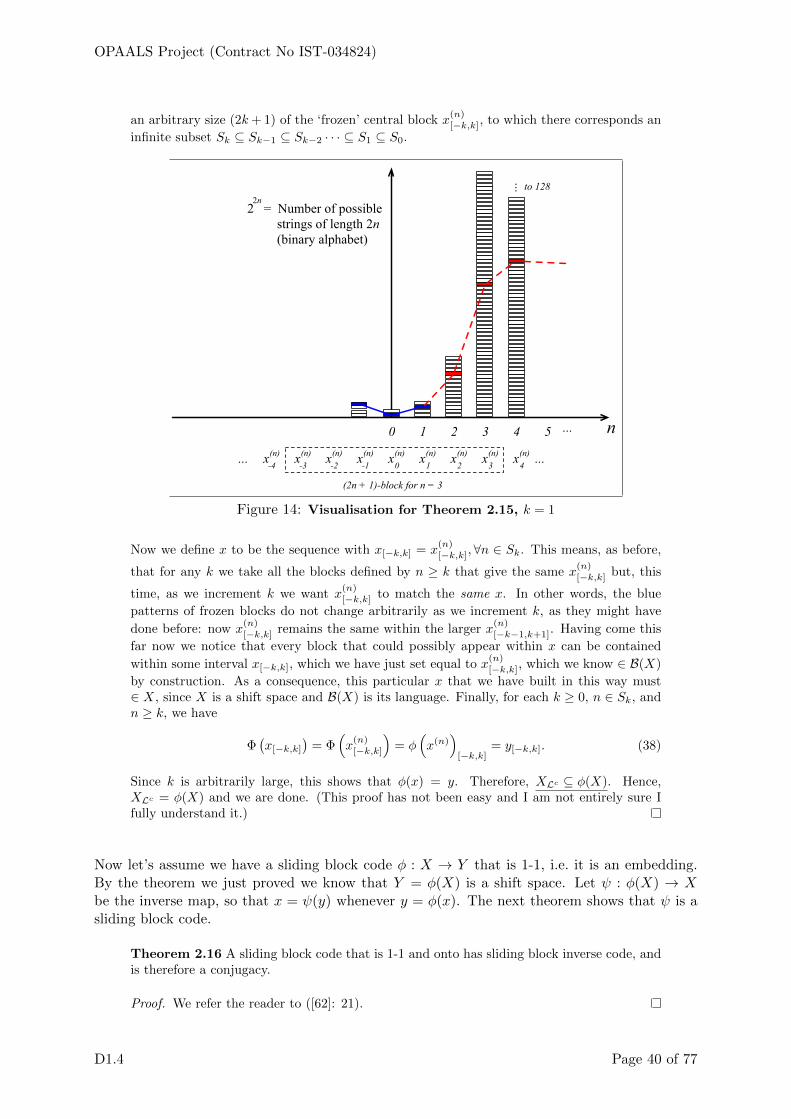
OPAALS Project (Contract No IST-034824)
an arbitrary size (2k+ 1) of the ‘frozen’ central block x(n)[−k,k], to which there corresponds an
infinite subset Sk ⊆ Sk−1 ⊆ Sk−2 · · · ⊆ S1 ⊆ S0.
n0 1 2 3 4 5 ...
... ...x x x x x x x x x(n)0 1 2 3 4-1-2-3-4
(n) (n) (n) (n) (n) (n) (n) (n)
(2n + 1)-block for n = 3
to 128...
2 = Number of possible strings of length 2n (binary alphabet)
2n
Figure 14: Visualisation for Theorem 2.15, k = 1
Now we define x to be the sequence with x[−k,k] = x(n)[−k,k],∀n ∈ Sk. This means, as before,
that for any k we take all the blocks defined by n ≥ k that give the same x(n)[−k,k] but, this
time, as we increment k we want x(n)[−k,k] to match the same x. In other words, the blue
patterns of frozen blocks do not change arbitrarily as we increment k, as they might have
done before: now x(n)[−k,k] remains the same within the larger x
(n)[−k−1,k+1]. Having come this
far now we notice that every block that could possibly appear within x can be contained
within some interval x[−k,k], which we have just set equal to x(n)[−k,k], which we know ∈ B(X)
by construction. As a consequence, this particular x that we have built in this way must∈ X, since X is a shift space and B(X) is its language. Finally, for each k ≥ 0, n ∈ Sk, andn ≥ k, we have
Φ(x[−k,k]
)= Φ
(x(n)[−k,k]
)= φ
(x(n)
)[−k,k]
= y[−k,k]. (38)
Since k is arbitrarily large, this shows that φ(x) = y. Therefore, XLc ⊆ φ(X). Hence,XLc = φ(X) and we are done. (This proof has not been easy and I am not entirely sure Ifully understand it.)
Now let’s assume we have a sliding block code φ : X → Y that is 1-1, i.e. it is an embedding.By the theorem we just proved we know that Y = φ(X) is a shift space. Let ψ : φ(X) → Xbe the inverse map, so that x = ψ(y) whenever y = φ(x). The next theorem shows that ψ is asliding block code.
Theorem 2.16 A sliding block code that is 1-1 and onto has sliding block inverse code, andis therefore a conjugacy.
Proof. We refer the reader to ([62]: 21).
D1.4 Page 40 of 77

OPAALS Project (Contract No IST-034824)
We originally meant to cover convolutional codes, since they fall within the framework of slidingblock codes, but lack of time is preventing us from putting our notes to LaTeX. We must presson with the next topic. We only have time to touch on shifts of finite type and then sofic shifts.
2.2.6 Shifts of finite type
Shift spaces described by a finite set of forbidden blocks are called shifts of finite type.Despite being the ‘simplest’ shifts, they play an essential role in mathematical subjectslike dynamical systems. Their study has also provided solutions to important practicalproblems, such as finding efficient coding schemes to store data on computer disks. Onereason why finite type shifts are so useful is that they have a simple representation using afinite, directed graph. Questions about the shift can often be phrased as questions about thegraph’s adjacency matrix. Basic results from linear algebra help us take this matrix apartand find the answers. ([62]: 28)
Definition 2.17 A shift of finite type is a shift space that can be described by a finitenumber of forbidden blocks.
If X is not a full shift, then it can also be defined by the complement of its language, X = XB(X)c .Since the complement of a language is infinite, this shows that a shift of finite type can also bedescribed by an infinite number of forbidden blocks. Definition 2.17 only says that there is somefinite F that is sufficient.
Since XF denotes the set of points x ∈ AZ that do not contain any blocks w ∈ F , as wedid in Proposition 2.9 we can easily define FN as a set of blocks of length N , where N is thelength of the longest block in F , and still say that XF = XFN
. If all the blocks have lengthN then any x ∈ AZ will belong to XF when x[i,i+N−1] /∈ F , ∀i ∈ Z; or, equivalently, whenx[i,i+N−1] ∈ BN (XF ). Here BN (XF ) is the set of all N -blocks that occur in XF . We don’t needto worry about smaller blocks because they are already contained in the allowed N -blocks. Forany block > N , the fractional part will fit in the next N -block. Hence knowing BN (XF ) issufficient.
Example 2.18: Even shift. This shift space is the set of binary sequences such thatbetween any two 1s there is an even number of 0s. Thus, for the even shift, F = {102n+11 :n ≥ 0}. This shift is not of finite type since F is not finite. If it were, there would be anN > 0 and a finite collection F of N -blocks such that X = XF . Having set that up, now letx = 0∞102N+110∞ (notice the capital N). Clearly, every N -block of x is in BN (X), leadingto x ∈ XF = X, contradicting the definition.
Shifts of finite type also have a memory.
Definition 2.19 A shift of finite type is M-step (or has memory M) if it can be describedby a collection of forbidden blocks all of which have length M + 1.
Since a single (M + 1)-block ∈ F appearing in a point x makes x ineligible, any M -step shift isalso a K-step shift ∀K ≥M . A 0-step shift is just a full shift, but with a smaller alphabet thanit started with. 1-step shifts of finite type can be seen as a collection of symbols together witha description of which symbols can follow them, like a Markov chain without probabilities.
Proposition 2.20 If X is a shift of finite type, then ∃M ≥ 0 : X is M -step.
Proof. Since X is of finite type, X = XF for some finite F . If F is not empty, let M be 1less than the longest block of F . We have already shown that X = XFM+1
, thus it is M -step.
D1.4 Page 41 of 77

OPAALS Project (Contract No IST-034824)
The next theorem sets the constraint to enable the splicing and joining of different segments,even belonging to different points of the same shift of finite type. The main concept is that forshifts of finite type words cannot necessarily just be joined end-to-end, they need to overlap aminimum amount. This theorem shows that this amount needs to be at least M .
Theorem 2.21 ([62]: 30) A shift space X is an M -step shift of finite type iff, wheneveruv, vw ∈ B(X) and |v| ≥M , then uvw ∈ B(X).
Proof. If X is M -step, then whenever uv, vw ∈ B(X) and |v| ≥M uvw ∈ B(X). F is madeof (M + 1)-blocks and is finite. Let uv, vw ∈ B(X), with |v| = n ≥ M . Then there are twopoints x, y ∈ X : x[−k,n] = uv, y[1,l] = vw and x[1,n] = y[1,n] = v. This is shown in Figure15.
... ...x x x x x x x x x0 1 2 n-1 n-1-k+1-k-k-1
... x-2
. ... xn+1
...y y y y y y0 1 2 n-1 n-1
... y-2
. ... yn+1
...y yl-1 l
yl+1
v
uv
vwM
Figure 15: Visualisation of overlap for splicing two points together, |v| ≥M
Now, we claim that the point z = x(−∞,0]vy[n+1,∞) ∈ X. This is because, since we knowthat v ∈ B(X) by assumption, if there were a block in z that ∈ F it would necessarily haveto be found in x(−∞,0]v = x(−∞,n] or in vy[n+1,∞) = y[1,∞), contradicting x ∈ X or y ∈ X.This is true as long as |v| ≥ M . The reason is not explained by Lind and Marcus probablybecause they consider it obvious, but it is actually a fairly subtle point. In essence, as shownin Figure 16, if |v| were smaller than M , then it would be possible for a forbidden blockto appear within uvw, and in particular across the xnyn+1 interface, because there is noguarantee that joining arbitrary symbols from different points will give an allowed block.
... x x x x x x x x y0 1 2 n n+1-1-k+1-k-k-1
... x-2
. ... ...yn+2
...y yl-1 l
yl+1
v
M
(∞, 0]x y...... [n + 1,∞)
Figure 16: Visualisation of overlap for splicing two points together, |v| < M
If whenever uv, vw ∈ B(X) and |v| ≥M uvw ∈ B(X), then X is M -step. More precisely,let F be the set of all (M + 1)-blocks over A that /∈ BM+1(X). If these blocks /∈ BM+1(X)then as we saw in Proposition 2.9 they or any of their subsets must belong to the original setof forbidden blocks (which might have been of variable length). So if we choose M so that(M + 1) matches the length of the largest forbidden block in the original set, we know thatF as defined here is a suitable set. We will show that X = XF , since that would be enoughto show that X is M -step.
If x ∈ X, then no block ∈ F can occur in x, so x ∈ XF . Therefore X ⊆ XF .
Now let x ∈ XF . Then any block ∈ x is also ∈ B(X). Thus, x[0,M ] and x[1,M+1] ∈ B(X).This is also because F contains only blocks of length M + 1. Since these two blocks overlap
D1.4 Page 42 of 77

OPAALS Project (Contract No IST-034824)
on M symbols, x[0,M+1] ∈ B(X) too. Now, x[2,M+2] ∈ B(X), and it overlaps with x[0,M+1] onM symbols. Thus x[0,M+2] ∈ B(X). Applying this argument recursively in both directionsgives x[k,l] ∈ B(X), ∀k, l ≥ 0. By Corollary 2.8.1, x ∈ X. Therefore, XF ⊆ X.
Hence, X = XF .
Theorem 2.22 A shift space that is conjugate to a shift of finite type is itself a shift of finitetype.
Proof. We refer the reader to ([62]: 31).
2.2.7 Graphs and their adjacency matrices
A method of constructing shifts of finite type that is interesting for us starts with a finite,directed graph and generates the collection of all bi-infinite walks, i.e. sequences of edges, onthe graph. It just so happens that every shift of finite type can be generated in this manner, i.e.as a so-called edge shift. Lind and Marcus explain that an edge shift can be understood muchmore easily than a general shift because we can apply powerful linear algebra techniques to itsadjacency matrix. We now list some definitions we need to develop the associated ideas.
• A graph G consists of a finite set V = V(G) of vertices, or states, together with finite set ofE = E(G) of edges.
• Each edge e ∈ E(G) starts at a vertex denoted by i(e) ∈ V(G) and terminates at a vertex t(e) ∈V(G) (which could coincide with i(e), creating a ‘self-loop’).
• We can also say that edge e has initial state i(e) and terminal state t(e).
• There may be more than one edge between i(e) and t(e) for a given e, creating a set of ‘multipleedges’.
• We may use the shorthand V and E for V(G) and E(G), respectively, when the context is clear.
• For a state I, EI = EI(G) denotes the set of outgoing edges, and EI = EI(G) denotes the set ofincoming edges.
• |EI | = ‘out-degree’ of I, |EI | = ‘in-degree’ of I.
Figure 17 shows a simple graph for which V = {1, 2, 3} and E contains 7 edges, labelled from a3-letter alphabet (not every state transition is defined in this example if interpret edge labels asinputs).
1
3
2
a b
bc
ba
a
c
Figure 17: Example of simple graph
D1.4 Page 43 of 77

OPAALS Project (Contract No IST-034824)
In order to define the adjacency matrix for a given graph, e.g. the example above, we need toorder the vertices or states, so we follow regular numerical or alphabetical order.
Definition 2.23 Let G be a graph with set of vertices V. For vertices i, j ∈ V, let Aij denotethe number of edges in G with initial state i and terminal state j. Then the adjacencymatrix of G is A = [Aij ], and its formation from G is denoted by A = A(G) or A = AG.For example, for the graph of Figure 17 the adjacency matrix is:
AG =
1 1 11 0 10 1 2
(39)
Definition 2.24 Let G be a graph with edge set E and adjacency matrix A. The edge shiftXG or XA is the shift space over the alphabet A = E specified by:
XG = XA ={ξ = (ξi)i∈Z ∈ EZ : t(ξi) = i(ξi+1),∀i ∈ Z
}. (40)
The corresponding shift map over XG or XA is called the edge shift map and is denotedby σG or σA.
This definition tells us that a bi-infinite sequence ∈ X when the terminal state of each edgeequals the initial state of the next edge. So, no discontinuous jumps are allowed.
Proposition 2.25 ([62]: 36) If G is a graph with adjacency matrix A, then the associatededge shift XG = XA is a 1-step shift of finite type.
Proof. If we list all the discontinuous jumps we will find all the forbidden blocks. Since wejust need 2 symbols to describe all such forbidden combinations of edges, and since for afinite alphabet there is a finite number of possible such combinations, we necessarily obtaina 1-step shift of finite type. Following Lind and Marcus’s more formal proof, let A = E bethe alphabet of XG. Consider the finite collection of 2-blocks of A:
F = {ab : a, b ∈ A, t(a) 6= i(b)} (41)
Definition 2.24 shows that a point ξ ∈ AZ lies in XG exactly when no block of F as definedhere occurs in ξ. Therefore, XG = XF , so XG is of finite type. Since all blocks in F havelength 2, XF is 1-step.
Although the shifts of finite type introduced so far are rather special, since for example theyhave no memory (the next state depends only on the current state, not on the previous historyof the sequence), the higher block representation we discussed in Section 2.2.4 enables us torecode any shift of finite type to an edge shift as defined here.
There are several more important results about graphs, such as homomorphisms and isomor-phisms, essential graphs, subgraphs, characterisation of path properties in terms of matrixproperties, irreducibility, etc, but we need to press on in order to reach a high-level understandingof the potential links between symbolic dynamics and automata theory.
2.2.8 Sofic shifts
This section will unfortunately be very short, as we ran out of time. We use Williams again [97]to sum up a few important points. A homomorphism from one shift to another is a continuousmap φ that commutes with the shift map. An onto homomorphism is called a factor map (or
D1.4 Page 44 of 77

OPAALS Project (Contract No IST-034824)
quotient map). An isomorphism between shift spaces is also called a conjugacy, which wehave already encountered and defined formally. We have not proven the Curtis-Hedlund-Lyndontheorem but we state it here: every homomorphism between shifts is given by a sliding blockcode. Another result that we have instead proven is based on the higher block shifts and statesthat that every shift of finite type is conjugate to a 1-step shift of finite type. This is apparentlya very useful device in constructing proofs as it allows us to reduce general arguments aboutsliding block codes to the case of 1-block codes. In contrast to Theorem 2.22, the homomorphicimage of a shift of finite type is not necessarily a shift of finite type. For example, the even shiftis not of finite type even though it can be obtained from the golden mean shift, which is. Theclass of homomorphic images of shifts of finite type that are shifts of finite type are called soficshifts.12 Since every shift of finite type is conjugate to an edge shift, sofic shifts correspond tofinite-state automata and in particular to regular languages.
We have to leave the discussion here, to be continued in the next publication on interactioncomputing, after the OPAALS project. After covering sofic shifts in some depth, we willattempt to connect them formally to the material in Chapter 4 on algebraic automata theory.On the strength of that connection we will seek an algebraic formalisation of algorithmsthrough symbolic dynamics compatible with interacting automata harbouring specific algebraicstructures.
Having shown how symbolic dynamics can help us analyse dynamical systems, and havingintroduced the p53-mdm2 system from the point of view phase space trajectories, the nextchapter looks at the p53-mdm2 system experimentally. Rather than focussing on its dynamicalsystem properties, which was already done in D1.3 [15], the work reported looks at the nextstep in the research on this regulatory pathway, towards a family of potential cancer drugs.Although the formal connections to this chapter and to Chapter 4 are not evident, they are noteven explored, for the moment. The experimental work leads the theoretical work by 1-2 years,so that we will probably use these results in future research efforts, after OPAALS.
12Sofic shifts were discovered by Weiss, an Israeli mathematician, and ‘Sofic’ in Hebrew means finite.
D1.4 Page 45 of 77

OPAALS Project (Contract No IST-034824)
3 Therapeutic Exploitation of the P53-Mdm2 Network
The OPAALS research in bio-computing, and in particular in gene expression-inspired comput-ing, has been carried out in part as a long-term dialogue among the authors of this report. Thecontributions of the UNIVDUN partner13 to WP1, WP12, and more recently to WP3 has beenmainly of three kinds:
• Theoretical and philosophical work in seeking connections between natural science epistemologiesand social science epistemologies.
• Numerical and mathematical work in the construction and evaluation of models for a particularregulatory pathway, the p53-mdm2 system, whose malfunction is fundamentally related to theonset of most cancers.
• Experimental cell biology work aiming to increase our understanding of this system and motivatedby the applied objective of developing new cancer drugs that interact directly with this regulatorypathway.
The second and third bullet are the more relevant to gene expression computing. A discussion ofthe p53-mdm2 system has already been provided in [15]. The character of the work is such thatexperimental research tends to lead theoretical and mathematical model development. Thus, inthe other chapters of this report we discuss connections between dynamical systems, symbolicdynamics, and algebraic automata theory and the p53-mdm2 system models and experimentalresults presented in previous reports and articles [14, 15, 16, 56, 21, 89]. The material discussedin this chapter, on the other hand, reports on recent experimental work that has receivedinternational recognition [57] and that has led to the identification of a potential new family ofdrugs, the Tenovins, but that we have not yet attempted to model mathematically.
3.1 Introduction
The TP53 tumour suppressor gene is the most commonly mutated gene in human cancers.The p53 protein itself, which is encoded by TP53, is inactivated in about 50% of adult solidtumours, whereas in the remaining 50% the function of p53 is totally or partially impaired bymodifications in other proteins within the p53 pathway. In order to explain p53’s biologicalfunction and the therapeutic implications thereof, we will first introduce some key concepts andterminology (summarised in Table 1) related to the process of protein synthesis. The chemicalcomposition of each protein is encoded by a specific gene, of which one or more copies can existin the genome. During the first step of the synthesis of a protein, known as transcription, thegene sequence is ‘read’ and copied in the form of a messenger RNA sequence (mRNA). Thisprocess is tightly modulated, for instance by the binding or so-called transcription factors to thepromoter region of the gene. Next, some fragments of the mRNA molecule can be ‘reorganised’,which means that a single gene can encode for more than one kind of protein. Then, the mRNAsequence is ‘translated’ once again, this time into the amino-acid sequence that constitutes thebasic chemical composition of the protein. Finally, this amino-acid sequence is generally ‘edited’,by chemical changes (i.e. post-translational modifications), and ‘folded’ in three-dimensions togive rise to a fully functional protein.
13The UNIVDUN team is composed of cancer biologists and cancer doctors from the University of Dundee,some of whom (Sonia Lain and Inge Van Leeuwen) have now moved to Karolinska Institutet in Sweden.
D1.4 Page 46 of 77

OPAALS Project (Contract No IST-034824)
PROCESS KEY PLAYERS DESCRIPTIONTranscription Genes,
Promoters, RNA-polymerases,Transcriptionfactors
RNA-polymerases ‘read’ the DNA code of a gene andproduce a complementary mRNA sequence. Tran-scription factors, which are proteins that bind to thepromoter region of specific target genes, regulate theactivity of the RNA-polymerases.
Splicing Spliceosome, In-trons, Exons
A protein complex known as spliceosome cuts noncodingfragments (introns) out of the original mRNA sequenceand combines remaining fragments (exons) into a finalmRNA molecule
Translation Ribosomes Ribosomes ‘read’ the mRNA sequence and use it tosynthesise a specific amino-acid chain.
Folding& Post-translationalmodifications
Chaperones Amino-acid chains generally need to fold, as well asundergo various chemical modifications, in order to giverise to a fully functional 3D protein structure. Thefolding process can be assisted by proteins known aschaperones.
Table 1: The basics of protein synthesis reminded
p53 executes its anti-cancer function by acting as a stress-inducible transcription factor14 asfollows. In response to a variety of potentially carcinogenic stimuli, such as exposure to radiationor DNA-damaging compounds, the p53 protein undergoes post-translational modifications15 andbecomes ‘active’ [63, 85, 88]. This more stable and transcriptionally active form then induces thesynthesis of a large number of target proteins, which carry out DNA repair, reversible cell-cyclearrest, irreversible cellular senescence or, when appropriate, programmed cell death [78]. Thefunction of p53 at the molecular level is summarised in Figure 18.
As p53 governs over the life and death of cells, it is not surprising that several layers of regulationtightly control its activity. The main regulator is mdm2 [71], an enzyme that keeps p53 levels lowin the absence of stress [46, 71]. Importantly, p53 and mdm2 are also linked by a transcriptionalfeedback-loop (Fig. 19), as MDM2 is a known p53 target gene [68, 98], that can cause p53levels to oscillate in response to stress [4, 9, 15, 43, 55, 89, 61, 72]. Interestingly, in tumourswith mutant p53, this feedback loop is absent, as the faulty p53 molecules are unable to actas transcription factors and therefore mdm2 levels remain very low. Consequently, cancer cellswith mutant p53 often present very high levels of the tumour suppressor.
Figure 18: Simpleschematic of p53’sfunction as a transcriptionfactor. The p53 tumoursuppressor is activatedin response to varioushazardous stimuli, suchas radiation, oxidativestress and viral infections.Active p53 then entersthe nucleus and regulatesthe expression of overa hundred target genes[34, 96].
14Concept defined in Table 115Concept defined in Table 1
D1.4 Page 47 of 77

OPAALS Project (Contract No IST-034824)
Figure 19: Negative feedback loop linking p53 andmdm2. The p53 tumour suppressor promotes thesynthesis of mdm2 [68, 98], while mdm2 proteinsbind to p53 and label it for degradation [46, 71].As protein synthesis (Table 1) is a relatively slowmolecular process, there is a so-called transcriptionaldelay in the feedback system. Both p53 and mdm2 arehighly-regulated proteins [54].
3.2 P53-based drug screening
P53, also known as the guardian of the genome [58], is arguably the one of most importantknown tumour suppressor in humans. In mice, transgenic animals lacking functional p53 presenta substantial increase in tumour incidence compared to wild-type animals [10, 45, 60]. Moreover,restoration of p53 function has been shown to induce growth inhibition in cultured cancer celllines [37, 86] and to cause regression of lymphomas and sarcomas in mice [95]. These observationsmake p53 a highly-attractive target for cancer therapy [8, 59]. There are currently two main linesof research regarding the therapeutic exploitation of p53 that aim at (1) ‘repair’ dysfunctionalp53 molecules in cancers with mutant p53, or (2) increase p53 levels in cancers with wild-typep53. Here we will focus on the latter kind of approach.
Large libraries of chemical compounds are now commercially available, which makes it possibleto perform high-throughput screens to identify potential new anti-cancer drugs. One possiblescreening approach is to seek compounds that interfere with a specific biochemical reaction. Invery simple terms, the involved proteins are purified, put in a test tube in suitable conditions,and then exposed to each compound in the library. This is known as reverse chemical genetic(RCG) approach or biochemical screening approach. In the case of the p53 pathway, for instance,an obvious way to try to enhance p53’s activity is to impede mdm2’s down-regulating function[91, 92]. A chemical screen for p53-activators based on this principle led to the successfuldiscovery of the nutlins, selective small-molecule activators of p53 [93]. The nutlins have beenshown to be capable of inducing up to 100% growth inhibition in various tumour models in mice.
The RCG approach above has some intrinsic limitations, including the following. Firstly, itrequires that the target, for example the mdm2–p53 interaction, is chosen beforehand. Secondly,it has to be possible to purify all components involved in sufficient amounts for the screen andto get the reaction of interest taking place in a test tube. Thirdly, a compound that constitutesa hit in the test-tube assay might not work in cells. It could, for instance, be highly toxic,incapable of entering the cell or rapidly degraded. An alternative way of screening compoundsis to seek for a desired biological effect, such as the activation of the p53 tumour suppressor,without worrying beforehand about how this effect occurs. This approach is known as forwardchemical genetic (FCG) approach, or cell-based screen, and has the great advantage that hitcompounds emerging from the screen are known to work in cells and are non-toxic. The maininconvenience or challenge associated with this approach is, however, that the mechanisms ofaction of the hit compounds are unknown. For example, a hit compound from a screen for p53activators could act directly on p53 itself or on any other protein modulating p53’s activity.Recently, a p53-based FCG approach has lead to the successful discovery of the tenovins [57], afamily of small-molecule activators of p53, and the JJ78 family [87], novel tubulin poisons withclear anti-tumour activities. The former molecules constitute the subject of the next section.
D1.4 Page 48 of 77

OPAALS Project (Contract No IST-034824)
3.3 Discovery & characterisation of the Tenovins
In 2008, Lain and co-workers [57, 67] screened a small-molecule library for p53 activators. Forthis purpose, they seeded cells onto 96-well plates and exposed them to the different compoundsin the library. To facilitate the detection of changes in p53 activity, the authors chose fortheir study a genetically-modified mouse cell line that expresses the lacZ gene, coding for aprotein called β-galactosidase (β-gal), under a p53-dependent promoter16. This means that theβ-gal enzyme is only present when p53 is acting as a transcription factor. Importantly, β-galactivity can be readily measured via a simple CPRG test, as CPRG cleaved by β-gal gives apink product that can be quantified by spectrophotometry. That is, expressed in lay terms,the p53-activating ability of chemical compounds can be evaluated based on the appearanceof a pink colouring. This is illustrated in Fig. 20A for actinomycin-D, a known activator ofthe p53 tumour suppressor. In the absence of actinomycin-D the (control and DMSO) wellspresent a yellow colouring, which corresponds to uncleaved CPRG, whereas in the presence ofactinomycin-D the wells acquire a pink colouring. Beyond a concentration of 50nM, however,actinomycin is toxic to the cells and, consequently, there is less β-gal activity and thus less pinkproduct. Fig. 20B shows a plate from an actual drug screen based on the same technique.
Figure 20: (A) Results from a p53-activation assay. Genetically-modified mouse cells wereseeded on a 96-well plate, left two grow for two days, and then treated with differentdoses of actinomycin-D (two wells per dose). The presence of p53-activity was revealedby the emergence of a pink colouring following incubation with CPRG mix (for detailedexperimental protocol, see [57]). Maximum p53 activity was achieved at ActD 25nM and50nM. Note that the intensity of the colouring starts to decrease at doses beyond 50nM,as then actinomycin-D becomes increasingly toxic for the cells.(B) Application of the same technique during a drug screen. Each well in columns 1 to11 was treated with a different compound from a chemical library. In column 12, the first4 wells were exposed to a negative control (DMSO), whereas the remaining were treatedwith a positive control (20nM ActinomycinD). The highlighted plate reveals two clear-hitcompounds, i.e. substances that activate the p53 tumour suppressor, in wells A4 and G8.
A screen of 34 000 small-molecules based on the primary cell assay shown in Fig. 20 yielded aninitial hit rate of about 2%. These 623 compounds were further tested (for technical details, seeSupplemental Data in [57]), for instance using different concentrations, and prioritized accordingto their performance. These secondary assays led to a final pool of 31 compounds of interest. In
16Concept defined in Table expression
D1.4 Page 49 of 77

OPAALS Project (Contract No IST-034824)
what follows, we will focus on the characterisation of one of them, which was coined tenovin-1.In cell culture, Western Blot analyses17 demonstrated that this compound is able to increasep53 protein levels substantially in less than two hours exposure. Moreover, both protein andmRNA18 levels were increased for various known p53 targets, such as the p21 protein, meaningthat p53 is transcriptionally active [57]. The levels of p53 mRNA, however, were the same inuntreated and tenovin-treated cells, which suggests that this compound increases p53 levels notby promoting its synthesis but by enhancing its stability.
Next, tenovin-1’s anti-tumour potential was tested on several cancer cell lines. Long-termtreatment (4 days) induced cell death and decreased cell growth in all of them [57]. TheARN8 melanoma cell line, which was particularly sensitive to tenovin-1, was selected forxenograft studies, where human cancer cells are implanted onto mice that have a deficientimmune system. Tenovin-1’s water solubility, however, turned out to be too low for use in vivo.Therefore, collaborators at the School of Chemistry at the University of St. Andrews modifiedthe chemical structure of tenovin-1 by adding a solubilizing group. The resulting compound,tenovin-6, not only conserves tenovin-1’s p53-activating properties, but even is slightly moreeffective. Importantly, the growth of ARN8-derived tumour xenografts was significantly reducedin tenovin-6 treated mice [57]. These promising observations convinced Lain et al (2008) thatis would be well-worth trying to identify the mechanism of action of tenovin-6.
The sensitivity of a cell to chemical compounds depends on how much of the target protein ispresent which, in its turn, depends on the number of copies of the gene encoding for it. Forinstance, lets consider a compound X that inhibits the activity of an enzyme-Y. Then cellsbearing only one copy of the Y gene, instead as the usual two copies, are likely to present lowerlevels of Y , which possibly renders them hypersensitive to X. Hence, in order to identify themolecular target of tenovin-6, Lain et al. [57] used a collection of more than 6000 genetically-modified yeast strains, each of which has one copy of a particular gene missing. Among thosestrains that were most sensitive to tenovin-6 was the one carrying a SIR2 deletion. This was avery interesting discovery, as SIR2 is the yeast homolog of mammalian proteins called sirtuins,which are involved in both ageing and cancer [90]. Furthermore, one of the sirtuins, SirT1 isknown to carry out post-translational modifications19 of various substrates, including the p53tumour suppressor [94]. It was thus well possible that tenovin-6 affects p53 activity by targetingSirT1. Indeed, two mammalian sirtuins, SirT1 and SirT2, were confirmed as targets of tenovin-6in in vitro biochemical assays using purified proteins.
Figure 21 summarises the interplay between p53, mdm2, sirtuins and tenovin-6. In the absenceof stress, mdm2 binds to p53 and labels it for degradation by adding so-called ubiquitin groups top53’s structure. As a consequence of this mdm2-mediated modification, p53 becomes less likelyto undergo an alternative post-translational modification20 consisting of the addition of acetylgroups. The levels of acetylated p53 are down-regulated further by SirT1, which is an enzymethat removes acetyl groups from its substrates. In the presence of stress, p53 becomes acetylated,which increases its stability, by preventing mdm2-mediated ubiquitination, and enhances itsactivity as a transcription factor [63, 88]. Finally, tenovin-6 promotes p53 acetylation andstability by inhibiting SirT1’s deacetylase function. That is, tenovin-6 affects the behaviour ofthe p53 pathway as a dynamical system. In the absence of stress, the reactions (represented byarrows) tend towards the left of in panel 21.A. In this context, p53 is preferentially degraded and,in particular, does not induce the synthesis of target proteins, including mdm2. Consequently,the levels of both p53 and mdm2 remain low. In contrast, in the presence of an oncogenic
17A method to quantify the total amounts of specific proteins in a cell population18Concept defined in Table 119Concept defined in Table 120Concept defined in Table 1
D1.4 Page 50 of 77

OPAALS Project (Contract No IST-034824)
stimulus, p53 becomes protected against mdm2 and, therefore, the reactions in panel 21.Btend towards the right. That is, in this context, p53’s tumour function as a transcriptionfactor is being promoted. Finally, exposure to tenovin-6 has comparable effects, as it preventsthe inactivation of active p53, thereby causing accumulation of p53 in its active form and theexpression of target genes.
Figure 21: Schematic sum-marising the mechanism ofaction of the tenovins.(A) In the absenceof stress, mdm2 addsubiquitin groups to thep53 molecule, targetingit for degradation. SirT1removes acetyl groupsfrom any ‘active’ p53molecules [94], whichbecome inactive andvulnerable to mdm2-medited degradation.In sum, under thisconditions, p53 is unstable,its levels remain very low,and the p53-target genesare not expressed.(B) In the presence ofstress, p53 undergoeschemical modifications,such as acetylation andphosphorylation, thatenhance its performanceas a transcriptionfactor and also preventdownregulation by mdm2[63, 85, 88]. In sum, underthese conditions, p53 isboth stable and active,and the p53-target genesare expressed.(C) Tenovin-6 inhibitsSirT1 function [57],thereby promoting theaccumulation of acetylatedp53 and thus indirectlyinterfering with mdm2sdownregulating function.In sum, tnv6 mimicsthe presence of stress byincreasing the levels ofactive p53, leading to theexpression of p53 targetgenes.
Having gained greater familiarity with the p53-mdm2 system, in the next chapter we go backto an algebraic perspective, and in particular to algebraic automata theory. At the end ofthe chapter we apply the computational algebra tools developed in Year 4 of OPAALS to thep53-mdm2 system.
D1.4 Page 51 of 77

OPAALS Project (Contract No IST-034824)
4 Algebraic Structure Analysis of Dynamical Systems
The work reported in this chapter builds on approximately 50 years of research in algebraicautomata theory, some of which was performed by researchers who founded the field and whoare still actively collaborating with the UH team. We can only skim the surface of this huge fieldin this short chapter, but we have taken pains to make the concepts accessible and to highlightthe contributions provided during the final year of the OPAALS project.
In spite of its overall accessibility, the material discussed in this chapter is very advanced, andcan therefore benefit from some context-setting remarks. In particular, in the DBE, BIONETS,and OPAALS bio-computing research activities we have always emphasised the importance ofsymmetries in the search for a model of computation that can construct order automatically,through interacting software artefacts. A symmetry is an invertible transformation that leavessome feature of a mathematical object invariant. Because the set of invertible transformationsof a mathematical object that leave some feature of that object invariant always form a group,we have always stressed that, whatever form the solution to the bio-computing problem mighttake, it would have to have a strong link to algebra.
The discrete nature of digital systems has motivated us to keep pushing for a bridge betweendynamical models of biological behaviour based on continuous mathematics, on the one hand,and behaviour specification languages for software engineering, on the other. The ‘stuff’ of thebridge itself appears to require the integration of an algorithmic or behavioural perspective witha state-set or structural perspective, both cast in discrete-mathematical or algebraic language.The symbolic dynamics discussion of Chapter 2 addresses the former, whereas this chapteraddresses the latter.
4.1 Introduction
4.1.1 Basic concepts
Readers who are unfamiliar with discrete group theory can find explanations of some of theelementary concepts in previous BIONETS and OPAALS reports and articles [22, 16, 20, 21,56, 83, 24]. To begin our discussion of algebraic automata theory we need to understand theconcept of transformation semigroup. This is most easily done by analogy with groups, as shownin Figure 22. Transformation semigroups are the mathematical objects that model automata.We are only concerned with the finite variety, meaning finite semigroups operating on finite setsof states [81].
Abstract group
Permutation group
Abstract semigroup
Transformation semigroup
Set of objects for which the concept of inverseis defined and with an operation between themsatisfying the associative and closure properties
Set of objects for which the concept of inverse is notnecessarily defined and with an operation between
them satisfying the associative and closure properties
Abstract group operating on a set of objects (e.g. states) Abstract semigroup operating on a set of objects (e.g. states)
Figure 22: Definition of basic terms
D1.4 Page 52 of 77

OPAALS Project (Contract No IST-034824)
It is helpful to fix these basic ideas with a couple of pictures. Figure 23 (which reproduces Figure12 of [22]) shows a comparison between an abstract group and a permutation group, while Figure24 (reproducing Figure 49 of [83]) gives a sense of what is involved with semigroups.
GroupGroup of transformations
Set of elements (or states)
b) Abstract group
Operation Composition
Set of elements,which can be anything
Set oftransformations
a) Original definition ofgroup, or modern definition
of permutation group
Set of elements (or states)
Ω Ω
G
G
c) More detailed depictionof permutation group
G
Figure 23: Comparison of abstract group with permutation group
s 2 ks s k + 1s
Number ofelements in
cycle = l
k + ls
k + l - 1s
k + l + 1s
k + 2s
k + 3s
3s 4s
ns
s 2s 3s 4s
l = 22k = 4n = l = 22
5s 6s
22s
s 2s 3s 4s 5s 30s
l = 4 k = 30 m = 8 n = ml = 32 32s
QState set
Subsets of states permuted bycyclic groups embedded insemigroup S acting on Q
Idempotent of element s
Trajectory of states acted uponby the 'tail' of a cyclic group
Figure 24: Visualisation of different possible collections of semigroup elements, showinghow cyclic groups can be embedded in a semigroup. Also shown is the set of states Qbeing acted upon, with a few representative state trajectories. Black dots: non-invertibleelements; blue and red dots: invertible elements. For a more detailed discussion, see [83].
D1.4 Page 53 of 77

OPAALS Project (Contract No IST-034824)
If S is a semigroup, the element s ∈ S is idempotent iff s2 = s. The concept of idempotentcan be seen as a generalisation for semigroups of the identity element for groups, althoughsemigroups can have, independently, also an identity element. Any kind of group, not just cyclicgroups as depicted in the figure, can be found in a semigroup. In particular, the simple non-abelian groups (SNAGs) are very interesting from the point of view of functional completenessand alternatives to Boolean algebra as a basis for computation [50]. After these preliminaryremarks we can start the discussion of the algebraic structure analysis of dynamical systems.
4.1.2 Motivation
Our ultimate goal is to understand and to engineer dynamical systems. By ‘engineer’ wemean the ability to predict and manipulate their behaviour, i.e. to influence their dynamicsin order to reach some target state of the system, or some target behaviour (e.g. a desiredlimit cycle). We can view dynamical systems from different perspectives but, once we handlethem as discrete state transition systems, then collapsings of states or cycles in state space andtheir intricate interrelations become the primary objects of study. Therefore algebraic automatatheory becomes a useful tool for identifying subsystems and discovering their relationships, andfor formulating this knowledge in a way that supports creative manipulation. Briefly, we callthese activities a coordinatization.
Hierarchical coordinate systems can obviously be used for dynamical systems, but not directly.As shown in Figure 25, which builds on Figure 5, we have to go through several intermediate stepsin order to get an automaton description of the given dynamical system. These intermediatesteps may involve technical difficulties (e.g. increasing the size of the state space, or there may bedifferent alternatives for doing one step that possibly yield radically different coordinate systems,as in a Petri net-to-finite-state-automaton conversion [29]). Therefore, the long-term goal is tofind the ways in which hierarchical coordinates can be used directly for dynamical systems. Forworking towards this goal, we need to make conceptual and technical advances in dealing withhierarchical coordinatizations.
DynamicalSystems
Algebra
SymbolicDynamics Automata
Theory
CodingTheory
HierarchicalCoordinatization
?
Figure 25: Finding the shortcut for applying the findings of algebraic coordinatization todynamical systems
One of the biggest achievements here is the development of SgpDec, the open-source algebraicsoftware package for cascaded structures and group and semigroup decompositions. This packageis written for the GAP open-source computer algebra system which currently contains the mostadvanced and most efficient computational group theory algorithms. The current version ofSgpDec is the culmination of several years of research and software development. During the
D1.4 Page 54 of 77

OPAALS Project (Contract No IST-034824)
OPAALS project its usability and scalability improved to a level that opens up a whole rangeof new possibilities in applied algebraic automata theory.
Constructive mathematical proofs are basically algorithms, but mathematical proof may neglectcomputational feasibility issues. The holonomy proof [99, 100, 33, 41, 48, 23] of Krohn andRhodes’s prime decomposition theorem for finite semigroups and machines [53] is the closestone to a computer scientist’s way of thinking. The holonomy coordinate system arises from adetailed analysis of how the semigroup acts on those subsets of the state set that are images ofthe state set under the action of the semigroup.21 Roughly speaking, a new level in the hierarchyappears when there is some irreversible step in the dynamics (e.g. collapsing two or more states).Symmetries may appear when there is a set of subsets of the state set that are mutually reachablefrom each other. The existence of these local pools of reversibility is a necessary but not sufficientcondition for the existence of nontrivial group components. Symmetries are periodic reversibilityoperations rather than just resets, thus the semigroup should act on these local pools in a specialway (capable of periodic returns in a nontrivial cycle) in order to form group components. Formore details see [28].
4.1.3 Algebraic Automata Theory
The hierarchical composition (cascade product) is a proper balance between two conflictingrequirements: having a nice, comprehensible structure and possessing the expressive powerto construct any arbitrary automaton. The parallel composition (direct product) has a verysimple structure, all of its components are completely independent, but this also means thatit is not possible to surpass the complexity of the building blocks. On the other hand, ifwe allow arbitrary wiring of the components (feedback loops with different lengths) then anysystem is realizable (even using only flip-flops as building blocks – see, e.g. [23]), but sucha construction generally provides no insight into structure or dynamics. In contrast, with acascaded decomposition, feedbacks in the original automaton being decomposed can give riseto structural permutation groups – possibly at different levels in the hierarchical decomposition– reflecting local symmetries in the system (i.e. acting on a subset of the state set). An easyexample would be a set of identical components with two states {0, 1} put into a directed loop(in other words the components form a line but the last element has a feedback to the first one)and a global operation that locally resets the state to 1 if the predecessor is in state 1, otherwisethe updated state is 0. This operation applied to the state vector (1, 0, . . . , 0) repeatedly createsa cyclic permutation.
For explaining Krohn-Rhodes Theory, the best way is to present it by using a metaphor.Basically we do the same thing that the decomposition into prime factors does for the integernumbers, but instead of integers we do it for more complicated structures, namely finite-stateautomata considered as transformation semigroups (see Figure 26).
The basic building blocks are (1) the simple22 permutation groups (for the reversible computa-tion) and (2) a single additional building block for the irreversible computation, the so-calledflip-flop automaton, which is essentially a one-bit resettable memory that can be set and read.23
The simple groups are called the ‘primes’ of this theory, as they play a role analogous to the
21Also included in what the semigroup acts upon are the singletons and whole state set, whether or not theyare images.
22This has a well-defined meaning in group theory: a group is simple if it has only trivial homomorphic images,i.e. any structure preserving map to another group is either one-to-one or collapses all elements to a single point.Alternatively, a group is simple if it has no normal subgroups. See, e.g. [82].
23An important but subtle point here is that although the flip-flop can be reset, this does not make it reversible.
D1.4 Page 55 of 77
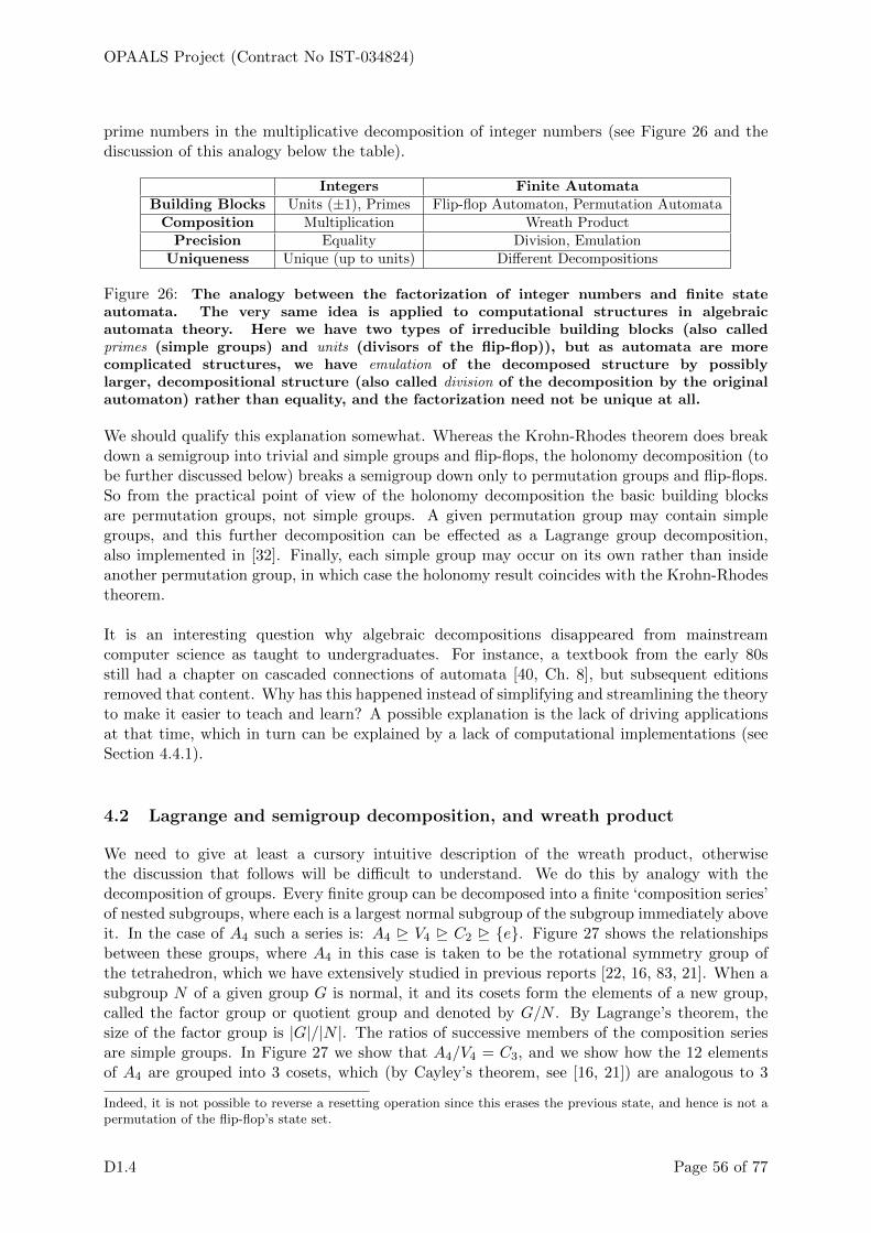
OPAALS Project (Contract No IST-034824)
prime numbers in the multiplicative decomposition of integer numbers (see Figure 26 and thediscussion of this analogy below the table).
Integers Finite AutomataBuilding Blocks Units (±1), Primes Flip-flop Automaton, Permutation Automata
Composition Multiplication Wreath ProductPrecision Equality Division, Emulation
Uniqueness Unique (up to units) Different Decompositions
Figure 26: The analogy between the factorization of integer numbers and finite stateautomata. The very same idea is applied to computational structures in algebraicautomata theory. Here we have two types of irreducible building blocks (also calledprimes (simple groups) and units (divisors of the flip-flop)), but as automata are morecomplicated structures, we have emulation of the decomposed structure by possiblylarger, decompositional structure (also called division of the decomposition by the originalautomaton) rather than equality, and the factorization need not be unique at all.
We should qualify this explanation somewhat. Whereas the Krohn-Rhodes theorem does breakdown a semigroup into trivial and simple groups and flip-flops, the holonomy decomposition (tobe further discussed below) breaks a semigroup down only to permutation groups and flip-flops.So from the practical point of view of the holonomy decomposition the basic building blocksare permutation groups, not simple groups. A given permutation group may contain simplegroups, and this further decomposition can be effected as a Lagrange group decomposition,also implemented in [32]. Finally, each simple group may occur on its own rather than insideanother permutation group, in which case the holonomy result coincides with the Krohn-Rhodestheorem.
It is an interesting question why algebraic decompositions disappeared from mainstreamcomputer science as taught to undergraduates. For instance, a textbook from the early 80sstill had a chapter on cascaded connections of automata [40, Ch. 8], but subsequent editionsremoved that content. Why has this happened instead of simplifying and streamlining the theoryto make it easier to teach and learn? A possible explanation is the lack of driving applicationsat that time, which in turn can be explained by a lack of computational implementations (seeSection 4.4.1).
4.2 Lagrange and semigroup decomposition, and wreath product
We need to give at least a cursory intuitive description of the wreath product, otherwisethe discussion that follows will be difficult to understand. We do this by analogy with thedecomposition of groups. Every finite group can be decomposed into a finite ‘composition series’of nested subgroups, where each is a largest normal subgroup of the subgroup immediately aboveit. In the case of A4 such a series is: A4 D V4 D C2 D {e}. Figure 27 shows the relationshipsbetween these groups, where A4 in this case is taken to be the rotational symmetry group ofthe tetrahedron, which we have extensively studied in previous reports [22, 16, 83, 21]. When asubgroup N of a given group G is normal, it and its cosets form the elements of a new group,called the factor group or quotient group and denoted by G/N . By Lagrange’s theorem, thesize of the factor group is |G|/|N |. The ratios of successive members of the composition seriesare simple groups. In Figure 27 we show that A4/V4 = C3, and we show how the 12 elementsof A4 are grouped into 3 cosets, which (by Cayley’s theorem, see [16, 21]) are analogous to 3
Indeed, it is not possible to reverse a resetting operation since this erases the previous state, and hence is not apermutation of the flip-flop’s state set.
D1.4 Page 56 of 77

OPAALS Project (Contract No IST-034824)
‘macro-states’. The next factor, V4/C2 = C2, ought to be shown as just two macro-states orcosets, {e, 4} and {9, 11}, but we are showing instead how the original group A4 gets partitionedinto 6 cosets. These 2 are in any case depicted as well. Finally, the Lagrange decomposition isunique up to isomorphism.
e
r
s
s
r r
s
s
r
r
r
s
s
r
r
r
r
r
s
s
r
s
s
s
s
2
3
4
5
67
8
910
11
12
r
r
r
s
ss
e
4 9
11
2
5 7
12
3
6 8
10
A4
V4
C2
{e}
A4 V4 C3=
V4 C2 C2=
e4 911
e 4
{e}
C2 C2=
s
s
s
s
r
r
r r
r
r
s
s
e 4
2 5
3 6
7 12
8 10
9 11
{e}
Figure 27: Visualisation of the Lagrange decomposition of A4
Figure 28 shows a hypothetical wreath product. The ovals indicate semigroups at different levelsin the decomposition, whereas the squares indicate the state sets present at the correspondinglevels. At any one level, a particular semigroup element (indicated by a letter) operates on theset of states at its same level, shown as a red arrow inducing the state transitions shown asgreen arrows. However, which semigroup elements operate depends on the states of the levelsabove through so-called dependency functions. The idea of the dependency functions is thatwhen a state transitions to another state at a given level (in response to e.g. a suitable input)this state transition may trigger the action of a semigroup element at the levels below. Thesetriggers are shown as dotted blue arrows. Similarly, the trigger on a semigroup element at agiven level may depend on state transitions happening at all the levels above, and not just atthe level immediately above. In order to be able to define a function, the latter perspective isadopted (as the former would not be single-valued).
In this example, we can recognise a cyclic group operating on 3 states at the second level (C3),and four C2 cyclic groups operating on the bottom level. This example is totally arbitrary andonly intended to provide a visualisation of the wreath product, so it’s not clear what automatonit corresponds to, if any. In the discussion that follows the letters X or Q denote the stateset, whereas the semigroup of transformations acting on the state set is denoted by S. Thus, atransformation semigroup is the ordered pair (X,S).
D1.4 Page 57 of 77

OPAALS Project (Contract No IST-034824)
4
5
13
2
67
8
9
jgi
h
fed
ab
cToplevel
3rdlevel
2ndlevel
Sets of states orof subsets of states
Sets of semigroup elements or ofsubsets of semigroup elements
Action of semigroupelement on set ofstates or macro-states
Dependency function
Legend
At each level, the rectangles denote sets of states orsets of subsets of states (aka macro-states). Thus, theaction of a semigroup on a set of states generates anested structure of states.
At each level, the ovals denote sets of semigroup elements. Eachelement could (but need not) be a set of elements of the level below.Thus a semigroup decomposition in the wreath product allows oneto describe its elements in a nested structure of transformations.
10
11
12
13
14
15
Figure 28: Visualisation of an element of a wreath product. The wreath product formalisesthe interaction between nested structures.
4.3 Conceptual advances
Decomposition theories usually provide an embedding of the original structure into a potentiallybigger composite structure. In the case of hierarchical decompositions the composite structureis a wreath product, which is in a sense a complete structure. Due to its size the wreath productcan easily become intractable. For instance, we can use the wreath product for coordinatizingC4, but we get a coordinate system of something bigger: C2 o C2
∼= D8, which is the group ofsymmetries of the square. The embedding obviously works C4 ↪→ D8, but the dihedral grouphas the flip-symmetry as well, beyond rotations. The discrepancy is relatively big and it getsbigger for groups with more elements. Therefore we aim to have more ‘economical’ coordinatesystems by using sub-wreath products.24 This is a slight change in viewpoint as decompositiontheories normally consider embedding into the wreath product (which as we said is usually avery big structure), but here we would like to put together the components more efficiently, thuswe study ‘sub-wreath’ products, that we call cascaded structures.
The problems are:
1. Wreath products have difficult definitions mostly in abstract algebraic terms.
2. Wreath products are huge structures, therefore computing with them is usually not possible dueto combinatorial explosion.
3. Due to their complexity, wreath products are difficult to grasp (except in some special cases) andthus they do not contribute to our understanding of the original automaton being modelled as acascade.
We suggest the following solutions:
1. Explicitly building the unidirectional connection network (dependency functions) between thecomponents.
24It is interesting that in the case of groups we can construct an isomorphic coordinate system, whereas this isnot the case for semigroups.
D1.4 Page 58 of 77

OPAALS Project (Contract No IST-034824)
2. Dealing with sub-wreath products.
3. Simplified visual notation for cascaded automata.
4.3.1 Dependency functions
In order to build cascaded structures with smaller combinatorial footprints we would liketo reduce the amount of wiring in the hierarchical structure. To achieve this here wedefine the connections between the components precisely. We fix a list of components L =((X1, S1), . . . , (Xn, Sn)
)where the indices correspond to depth values indicating the hierarchical
level, then
Definition 4.1 A dependency function di in L (of level i) is a function
di : X1 × . . .×Xi−1 → Si i ∈ {1 . . . n}. (42)
Thus a dependency function of level i has arity (i − 1). This includes the i = 1 case as well,when the dependency can be considered as a constant, a function with no arguments: {1} → S1.The intuitive interpretation of the dependency function is that it provides a set of rules withwhich one can pick an actual operation from a component based on the states of the componentsabove (an easily understandable example is provided in Section 4.3.3).
The wreath product contains all dependency functions for each level and all of their possiblecombinations, hence it keeps exploding combinatorially. However, constructive algorithms fordecompositions build ‘economical’ coordinate systems by using sub-wreath products, and in thecase of groups we can even construct an isomorphic coordinate system. Therefore, focusing ondependency functions and treating them as first class objects in implementations are importantconceptual steps.
4.3.2 Evolving and using new notations
In mathematics notation is an important issue. It can promote or hinder the understanding ofideas. Therefore we put special emphasis on choosing and developing the right notation.
Transformations of Finite Sets From early on, group theory had its specialized notation forpermutations, the cyclic notation, as it is easy to observe that a permutation consists of distinctcycles. On the other hand semigroup theory seems to be more reluctant to depart from theconventional 2-line matrix-like notation, which is rather space-consuming and makes recognizingthe salient features of transformations rather difficult. A new notation was introduced in 2005[3], then a more refined one in 2009 [38, Ch. 1.3]. We use the latter one with slight modificationsin order to obtain an even more compact notation.
Considering the mappings as digraphs, each transformation consists of one or more components.Each component contains a cycle (possibly a trivial cycle). Unlike the permutation case, thepoints in the cycle can have incoming edges, denoted by
[ source1, . . . , sourcem ; target ]
D1.4 Page 59 of 77

OPAALS Project (Contract No IST-034824)
1
4
6 2
35
8
7
Figure 29: Linear notation for a finite transformation: ([[1, 7; 4]; 6], 8)(3, 5). With this notationit is easy to see whether the transformation has a nontrivial cycle or not, one has to lookfor the round brackets. The traditional notation would be ( 1 2 3 4 5 6 7 8
4 2 5 6 3 8 4 6 ).
where target is the point in the cycle. If a source point also has incoming edges from other pointsthe same square bracket structure is applied again recursively. We can say that the points inthe cycle are sinks of trees. Parentheses indicate the existence of a nontrivial permutation ofthe sink elements of the trees, but not of their sources:(
[ sources1; target1 ], . . . , [ sourcesk; targetk ]).
This corresponds to the cycle( target1, . . . , targetk)
but at the same time it contains information on transient states. The order is arbitrary if thereis more than one component. Our notation is slightly different to [38] as we do not use squarebrackets for a singleton source. Moreover, for constant mappings we just use [→ n], where n isthe image. This modified notation is used in SgpDec. Here are some examples (for an exampleof a functional digraph see Figure 29):
• The cyclic notation is retained for permutations ( 1 2 31 2 3 ) = (), ( 1 2 3
2 3 1 ) = (1, 2, 3)
• An elementary collapsing looks like this: ( 1 2 33 2 3 ) = [1; 3]
• A ‘line’: 2 7→ 3 7→ 1 ( 1 2 31 3 1 ) = [[2; 3]; 1]
• A transposition with a third point collapsing into the cycle: ( 1 2 32 1 2 ) = (1, [3; 2])
• A constant: ( 1 2 31 1 1 ) = [→ 1].
4.3.3 Cascaded automata and abstract number systems
Integrating dependency functions arguments into the labels Cascaded operations canbe visualized in a tree format, where the paths are labelled by states from the corresponding leveland the nodes contain the local action (the value of the dependency function) [75]. However,this view displays only one element of the cascaded structure and thus a component of oneparticular level is scattered in several different diagrams (the number of generators). Thereforewe need a diagram that shows the components as automata and still retains information of
D1.4 Page 60 of 77

OPAALS Project (Contract No IST-034824)
the dependency functions. The idea is that we use a composite label for the state transitions:we augment the label of the cascaded operation with a coordinate tuple as the argument of itsdependency function on that particular level. So (x1, . . . , xi)a means that the cascaded operationa acts on component i+ 1 by the state transition that it labels. The basic idea was used alreadyin the late 60s but the state vector appeared explicitly in the label of a state transition first in[64] then it was used in [5]. For instance, in a cascaded structure, given the current states onthe first i levels are (x1, . . . , xi), xk ∈ Xk and we have a dependency function d giving the valuesi+1 = d(x1, . . . , xi), then for two states xi+1 and yi+1 of the i+ 1th level we will have a labelledarrow
xi+1 yi+1(x1, . . . , xi)d
supposing that xi+1 · si+1 = yi+1.
This concept can probably be explained more easily through the example of a simple binarycounter. Figure 30 provides such an example, but it is actually trying to achieve 4 thingssimultaneously:
• Provide an easily understandable example of what we mean by ‘coordinatisation’.
• Provide an example of the tiling notation (that will be discussed next) through a visualisation ofthe decomposition of the cyclic group of 16 elements, C16. Although the holonomy decompositioncannot be applied to a group and, therefore, such a tiling picture is not applicable, we are showing itanyway because it helps fix a couple of useful concepts that generalise to semigroup decompositions.
• Demonstrate the dependency functions through the familiar concept of the carry bit.
• Prepare the ground, therefore, for the introduction of the abstract concept of a finite-stateautomaton as defining a ‘customised’ generalised number system (to be discussed below).
{4,12} {2,10} {6,14} {1,9} {5,13} {3,11} {7,15}
1 1 0 1 + 1
0 1
+1
+1
0 1
(1) +1
(1) +1
0 1
(1,1) +1
(1,1) +1
0 1
(1,1,1) +1
(1,1,1) +1
1
0
1
1
0
1
1
1
= 1 1 1 0 {0,1,2,3,4,5,6,7,8,9,10,11,12,13,14,15}
{0,2,4,6,8,10,12,14} {1,3,5,7,9,11,13,15}
{0,4,8,12} {2,6,10,14} {1,5,9,13} {3,7,11,15}
{0,8}
{8}{0} {4} {12} {2} {10} {6} {14} {1} {9} {5} {13} {3} {11} {7} {15}
Figure 30: Coordinatisation of the numbers 13 and 14 expressed as two elements of C16
Since this figure is trying to accomplish so many things, it will take a little time to unpack.We start with the familiar binary addition of 13 + 1 = 14, which is shown on the left of thefigure. Each position in a positional number system can be seen as a different ‘coordinate’.
D1.4 Page 61 of 77
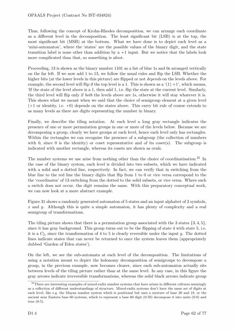
OPAALS Project (Contract No IST-034824)
Thus, following the concept of Krohn-Rhodes decomposition, we can arrange each coordinateas a different level in the decomposition. The least significant bit (LSB) is at the top, themost significant bit (MSB) at the bottom. What we have done is to depict each level as a‘mini-automaton’, where the ‘states’ are the possible values of the binary digit, and the statetransition label is none other than addition by a +1 input. But we notice that the labels lookmore complicated than that, so something is afoot.
Proceeding, 13 is shown as the binary number 1101 as a list of blue 1s and 0s arranged verticallyon the far left. If we now add 1 to 13, we follow the usual rules and flip the LSB. Whether thehigher bits (at the lower levels in this picture) are flipped or not depends on the levels above. Forexample, the second level will flip if the top level is a 1. This is shown as a ‘(1) +1’, which means,‘If the state of the level above is a 1, then add 1, i.e. flip the state at the current level. Similarly,the third level will flip only if both the levels above are 1s, otherwise it will stay whatever it is.This shows what we meant when we said that the choice of semigroup element at a given level(+1 or identity, i.e. +0) depends on the states above. This carry bit rule of course extends toas many levels as there are digits representing the number in binary.
Finally, we describe the tiling notation. At each level a long gray rectangle indicates thepresence of one or more permutation groups in one or more of the levels below. Because we aredecomposing a group, clearly we have groups at each level, hence each level only has rectangles.Within the rectangles we can recognise the presence of a subgroup (the collection of numberswith 0, since 0 is the identity) or coset representative and of its coset(s). The subgroup isindicated with another rectangle, whereas its cosets are shown as ovals.
The number systems we use arise from nothing other than the choice of coordinatisation.25 Inthe case of the binary system, each level is divided into two subsets, which we have indicatedwith a solid and a dotted line, respectively. In fact, we can verify that in switching from theblue line to the red line the binary digits that flip from 1 to 0 or vice versa correspond to thethe ‘coordinates’ of 13 switching from the dotted to the solid subsets, or vice versa. Where sucha switch does not occur, the digit remains the same. With this preparatory conceptual work,we can now look at a more abstract example.
Figure 31 shows a randomly generated automaton of 5 states and an input alphabet of 2 symbols,x and y. Although this is quite a simple automaton, it has plenty of complexity and a realsemigroup of transformations.
The tiling picture shows that there is a permutation group associated with the 3 states {3, 4, 5},since it has gray background. This group turns out to be the flipping of state 4 with state 5, i.e.it is a C2, since the transformation of 4 to 5 is clearly reversible under the input y. The dottedlines indicate states that can never be returned to once the system leaves them (appropriatelydubbed ‘Garden of Eden states’).
On the left, we see the sub-automata at each level of the decomposition. The limitations ofusing a notation meant to depict the holonomy decomposition of semigroups to decompose agroup, in the previous example, now becomes clearer, since each sub-automaton actually sitsbetween levels of the tiling picture rather than at the same level. In any case, in this figure thegray arrows indicate irreversible transformations, whereas the solid black arrows indicate group
25There are interesting examples of mixed-radix number systems that have arisen in different cultures seeminglyas a reflection of different understandings of structure. Mixed-radix systems don’t have the same set of digits ateach level, like e.g. the Mayan number system which is positional but uses a mixture of base 20 and 18, or theancient near Eastern base 60 systems, which to represent a base 60 digit (0-59) decompose it into units (0-9) andtens (0-5).
D1.4 Page 62 of 77

OPAALS Project (Contract No IST-034824)
elements, as provided by SgpDec. However, this example is simple enough that it can be doneby hand. In particular, the states of the sub-automaton at the top level is formed simply bythe image sets of the original state set {1, 2, 3, 4, 5} under the action of the two inputs. Thisis shown in Figure 32. Finally, the bottom level of Figure 31 shows how the state transitionsdepend on the system being in specific states in the level above.
1
2
3
4 5
x
y
y
y
y
xx
x,y
x
{1, 2, 3, 4, 5}
{3, 4, 5} {2, 3}
{2}{4}{3}{1} {5}
{3, 4, 5} {2, 3} 1
x
y
x
y
x
y
3
4
5({3,4,5}) y
({3,4,5}) x
2 3
({2,3}) y
({2,3}) x({1}) x
({3,4,5}) y
({3,4,5}) y ({2,3}) y
({3,4,5}) x
({3,4,5}) x({2,3}) x
({1}) x
Figure 31: Graphical notation for a randomly generated automaton (top right), theskeleton of its holonomy decomposition (tiling picture, middle) and the components ofthe hierarchical levels with the dependency functions (left).
{1, 2, 3, 4, 5} {3, 4, 5}
{2, 3}
3
x,y
x
x
x
y
y
y
1
2
3
4 5
x
y
y
y
y
xx
x,y
x
Randomly generatedautomatonTop-level state image sets
Figure 32: Obtaining the image sets for the top level from the original automaton
Taking a step back, we can see how we have treated this automaton in a way that is entirelyanalogous to a number, although in a rather more abstract way. The analogue of adding +1 toa binary number becomes the provision of an input symbol to the automaton. What made thenumber example of Figure 30 particularly simple is that the inputs and the states at each levelall came from the same binary alphabet. For a general automaton this is clearly not going tobe the case very often, if ever. Furthermore, at each level in a number expressed in a positionalnumber system we have one mini-automaton. In this automaton example, on the other hand, atthe bottom level two sub-automata are operating, each with its own state transitions; therefore,the bottom level is characterised by two states in parallel, which is a rather confusing way tothink of a number. Finally, each state of the automaton corresponds to a different number
D1.4 Page 63 of 77

OPAALS Project (Contract No IST-034824)
in the number system that the automaton defines. As a consequence, we reach the surprisingconclusion that from this abstract perspective there is no difference between ‘computing’ and‘counting’.
Hopefully the power of the coordinatisation perspective to uncover the inner structure ofautomata is becoming clear, in the sense that a lot more information is provided by thesediagrams relative to what one can evince from the original automaton. In any case, we noticean interesting parallel between this concept of an automaton as a generalised number systemand the same idea applied to dynamical systems, as discussed in Section 2.1.2.
One arrow for constant maps The components of the holonomy decompositions arepermutation-reset semigroups (groups together with constant maps for all states), thereforearrows for constant maps will be abundant in the diagram of the component automaton. Sincewe know that from all states there is always an arrow with the label of the constant map totarget state (the image of the constant map), there is no need to draw them explicitly. Instead,a short wide arrow can indicate the existence of a constant map. One objection may be thatin the case of a pure reset automaton the state transition diagram becomes disconnected, butactually this is desirable as the nonexistence of a group component is immediately clear.
1
2
3
4 5
x
y
y
y
y
xx
x,y
x{1, 2, 3, 4, 5}
{3, 4, 5} {2, 3}
{2}{4}{3}{1} {5}
{3, 4, 5} {2, 3} 1
y x
3
4
5({3,4,5}) y 2 3
({2,3}) y({3,4,5}) y
({3,4,5}) x({1}) x
Figure 33: Advanced graphical notation for the same randomly generated automaton. Thickarrows replace the arrows for a constant. The effect that the component automaton splitsup into disconnected pieces is desirable as it shows that the states are not connected by asymmetry operation.
In preparation for the more complicated examples discussed below, we show a very compactand low-resolution way to represent the semigroup decomposition of the random automaton.Figure 34 shows that this automaton is decomposable into just two levels. The 1 at the toplevel means that a trivial group is acting on the whole set of states {1, 2, 3, 4, 5} to generate thefirst level of image sets. ‘Trivial’ here means that nothing comes back, both x and y give riseto irreversible transformations. The second level shows the presence of another trivial group,i.e. the irreversible transitions into the subset of states {2, 3}, and a cyclic group of order 2. C2
refers to the permutation of states 4 and 5 under the action of the y input.
D1.4 Page 64 of 77

OPAALS Project (Contract No IST-034824)
1:2:
11 C2
Figure 34: Compact notation for showing the decomposition of the random automaton
4.4 Technical advances
4.4.1 History of Computer Implementations
No matter how sound the underlying theory, developing useful applications is impossible if wedo not have the practical tools to actually apply the theory. In the case of algebraic automatatheory the practical tool is a computational implementation of the holonomic decomposition ofarbitrary transformation semigroups. Unfortunately for the Krohn-Rhodes theory, there was noavailable computational tool for forty years. Therefore, except for special classes of automatawhere the decomposition can be established theoretically (e.g. full transformation semigroups,monogenic semigroups), some tedious hand calculations [81], and a few small example exercises[33], there was no possibility to study bigger examples of decompositions.
The first computational implementations were achieved at the University of Hertfordshire [27]and already surpassed the capabilities of pen and paper calculations, but they did not allowinteractive calculations and were difficult to use by non-experts. Therefore a decision was madeto include the semigroup decomposition package into the GAP computational algebra platform[39], the most advanced and open-source computer algebra system for computational grouptheory. The development started in 2006 but until the UH development team joined the OPAALSproject only the Lagrange decomposition [31] (for permutation groups) had been completed forthe software package. The new challenges in the OPAALS project required further advancementsin the software development and eventually led to a mature software package [32].
Currently, SgpDec[32] is capable of calculating decompositions of semigroups of size tens ofthousands (acting on around 50 states). This is beyond doubt a significant step towards realizingthe vision of ‘engineering’ dynamical systems.
4.4.2 Interactive computing for experimental exploration
Since computational implementations for algebraic decompositions are still experimental we putspecial emphasis on the interactive capabilities of the SgpDec package [32]. The calculations canbe done in smaller pieces and can be investigated or ‘splashed’, i.e. the automatically generatedfigures can be displayed immediately, supporting visualizations of the decompositions, cascadedoperations, as well as other structures.
4.4.3 Improving scalability
There are different ways of doing hierarchical decompositions of semigroups, but we are interestedin those dealing with transformation semigroups, as the state set can be considered as analogousto the phase space of a dynamical system. The holonomy decomposition works directly withthe state set, therefore it is the primary choice for a computational implementation. The
D1.4 Page 65 of 77

OPAALS Project (Contract No IST-034824)
decomposition itself is a complicated algorithm with several stages. We have improved scalabilityof the software in the following ways:
• Integrating functionalities from other GAP packages.
– The MONOID [70] contains the efficient orbit calculation algorithm used for producing theskeleton of the holonomy decomposition.
– The orb [74] package contains excellent hashtable functionality. Hashtables are used in manyplaces when we keep track of a growing set of elements.
• Using minimizations for sequences of state transitions by cutting off redundant loops. These‘straight words’ can be used for reducing memory footprint and processing time [25].
4.5 Experiments on the algebraic models of the p53-mdm2 system
For studying the p53-mdm2 system algebraically we start from a Petri net (Fig. 35). A discussionof this Petri net and of how it models the p53-mdm2 system can be found in [24, 89, 15]. Fromthe Petri net we can derive an automaton by fixing the capacities of the places (for the exactmethod see [29]), but increasing the capacities of the places can lead to automata with so manystates that they become impossible to handle due to scalability issues. The simplest case is whenwe only distinguish between the presence (above a certain threshold) and the absence of someparticular substrate (capacity 2). In this case we get an automaton with 16 states (Fig. 36)with a corresponding semigroup that has 316,665 elements and admits a 17-level decomposition(Fig. 37). This size may be too small for the model, the semigroup contains no SNAGs (simplenon-abelian groups). Fortunately, recent advances in the scalability of the SgpDec [32] packageallows us to study decompositions of bigger automata (Fig. 38).
M
P
R
C r8
r7 r6
r3
r5 r1
r2
r9
Ionising radiation
Degraded p53
r4
Figure 35: (A) Schematic of the p53-mdm2 regulatory pathway [89], and (B) correspondingPetri net [24]. P = p53, M = mdm2, C = p53-mdm2, R = p53*.
Table 2 summarises the salient features of the three examples we have examined.
It is clear that the next challenge is to find a way to reduce the number of levels, for exampleby compressing the information contained in the levels only with trivial group components.
D1.4 Page 66 of 77

OPAALS Project (Contract No IST-034824)
1000
1010t1
0000
t4
0001
0010
t7
0011
t11001
t3
t9
0100t8 1100
t3
0110
t1
t8
t4
1110
t1
t5
t2
1101
t6
t4
t8
t6
t3t2
1111
t7,t9
t2,t6
1011
t8
0101t5
0111t4
t9t7
t1
t8
t4
t4t2,t6
t7,t9
t5
t2,t6
t7,t9
t3
t9t4
t1t7
t2
t3t8
t6
t2
t5
t4
t6
t9
t3
t8
t7
t1
t3
t1
t3
t8
t7,t9
t2,t6
Figure 36: Automaton derived from 2-level Petri net of the p53 system (16 states). Thelabels on the nodes encode the possible configurations for M, C, P and R (in this order). 0denotes the absence (or presence below a threshold), 1 the presence (above the threshold)of the given type of molecule. For instance, 0101 means that C and R are present. Theshaded states correspond to the state set {3 = 1000, 5 = 0001, 8 = 0100}.
1:2:3:4:5:6:7:8:9:
10:11:12:13:14:15:16:17:
11111 11 11 1 11 1 1 11 1 1 11 1 1C211 11 1 1S31C2
Figure 37: The components of the holonomy decomposition of the 16-state p53 automaton.Each line corresponds to a hierarchical level, several components on the same level indicateparallelism within one level. The top level is 1, 17 is the lowest level. Level 17 dependson changes at levels 1 to 16, whereas the top level’s operation is independent of the statesof lower levels. The components are permutation-resets (a group augmented with constantmaps), but only the group components are indicated (the trivial group is denoted by 1).
D1.4 Page 67 of 77

OPAALS Project (Contract No IST-034824)
11 11 11 1 11 1 1 11 1 1 1 1 11 1 1 1 11 1 1 11 1 1 1 1 1 1 11 1 1 1 1 1 1 11 1 1 1 1 1 1 1 11 1 1 1 1 1 1 1 1 1 11 1 1 1 1 1 1 1 1 1 1 1 11 1 1 1 1 1 1 1 1 1 1 1 1 11 1 1 1 1 1 1 11 1 1 1 1 1 1 1 1 11 1 1 1 1 1 1 1 1 1 1 1 1 1 1 11 1 1 1 1 1 1 1 1 1 1 1 1 1 1 1 1 1 1 1 11 1 1 1 1 1 1 1 1 1 1 1 1 1 1 1 1 1 1 1 1 11 1 1 1 1 1 1 1 1 1 1 1 1 11 1 1 1 1 1 1 1 1 1 1 1 1 1 11 1 1 1 1 1 1 1 1 1 1 1 1 1 1 1 1 1 1 1 1 11 1 1 1 1 1 1 1 1 1 1 1 1 1 1 1 1 1 1 11 1 1 1 1 1 1 1 1 1 1 1 1 1 1 1 1 1 1 1 1 1 1 1 1 1 11 1 1 1 1 1 1 1 1 1 1 1 1 1 1 1 1 1 1 1 1 11 1 1 1 1 1 1 1 1 1 1 1 1 1 1 1S51111 1 11 1 1 1 1 1 1 1 1 1 11 1 1 1 1 1 1 1 1 1 1 1 1 1 1 1 1 1 1 11 1 1 1 1 1 1 1 1 1 1 1 1 1 1 1 1 1 1 1 1 1S3 1 1 1 1 1 1 1 1 1 1 1 1 1 1 1 1 1 1 1 1 1 1 1 1A5 1 1 1 1 1 1 1 11 1 1 1 1 1 1 1 11 1 1 1 11 1 1 1 1 11 1 1 1 1 1 1 1 1 1 1 11 1 1 1 1 1 1 1 1 1 1 1 1 1 1 1 1 1 1 1 1 1S411 1 1 1 1S3C2
1:2:3:4:5:6:7:8:9:
10:11:12:13:14:15:16:17:18:19:20:21:22:23:24:25:26:27:28:29:30:31:32:33:34:35:36:37:38:39:40:41:42:43:44:45:46:
Figure 38: Groups occurring at each level of the holonomy decomposition of a 36-statep53 automaton (having 3 different levels of concentration for M and C, whereas onlytwo different concentration thresholds are distinguished for P and R). A SNAG, A5, thealternating group on 5 points, does appear among the group components. Although S5 isnot a simple group, it is shown in red because it contains A5.
Random 16-State 36-StateAutomaton p53 System p53 System
Number of states 5 16 36Number of levels 2 17 46
Order Unknown, still being calculatedof 4 316,665 by a Mac server with 12GB RAM,
semigroup 260 hrs CPU time and counting...
Table 2: Comparison of characteristic dimensions of the automata examined
D1.4 Page 68 of 77

OPAALS Project (Contract No IST-034824)
5 Conclusion
5.1 Highlights of general results in interaction computing research 2003-10
Within the interaction computing research agenda, which started in 2002 with the preparationof the DBE project proposal, the main ‘discoveries’ to date have been the following:26
• Krohn-Rhodes theory [81] and the work of UH, who subsequently joined the project.
• The possible interpretation of the permutation groups of state subsets embedded within thetransformation semigroup of a given automaton as a mechanism for parallel, cyclic, and notnecessarily in-phase computation ([16]: 23-24; [24]).
• The theoretical framework connecting automata structure and behaviour, and automata behaviourand specification languages through category theory ([21]: 120; [81]: 57), shown in Figure 39.
• The realisation that global Lie symmetries are probably too restrictive to be applicable to theanalysis of metabolic pathways. As we mentioned in D1.3 [15] Lie groupoids are likely to behelpful here as they correspond to symmetries that are ‘local’ in some sense. For example,biological systems do not operate at all possible temperatures, but only over a fairly limited rangeof temperature. However, the type of mathematical thinking required is very different to whatwe have been working on in the past few years (with the exception of [12, 16, 51]). It seemsbest to focus on the discrete mathematics perspective of the present report, which is more likelyto bear fruit in the short term. Any such results could then be helpful also in developing a Liegroup/groupoid-based approach.
• The probable relevance of Ross Ashby’s Law of Requisite Variety [2] to the architecture of self-organising systems. In other words, the self-organisation of metabolic systems and the self-organisation of evolutionary systems might be seen as instantiations of this same abstract lawinto these two very different contexts. In both cases we would therefore expect to find a commonmathematical structure; for instance, a reliance of ‘local’ behaviour on ‘global’ context, where localand global are relative and recursive concepts in the sense that they apply to each pair of adjacentlayers in a nested hierarchy. The difference is that in the case of evolution the ‘nesting’ takes placealong the time dimension – and we call it ‘history’, or ‘memory’, or ‘path-dependence’ – whereasin the case of metabolic systems it takes place along an axis that measures system scale. Thus,from the point of view of the law of requisite variety metabolism could be seen as a ‘projection’ ofevolution along the time axis and onto the ‘plane’ perpendicular to the time axis that defines ‘now’(thereby resurrecting a strange form of recapitulation [18]). In both cases, in fact, we observespontaneous order construction of unbelievable complexity, but on totally opposite time-scales.The fact that the dynamical self-organisation of metabolic and other real-time systems appearsto depend on a non-linear mathematical structure could then be explained by the fact that non-linearity provides the coupling between different degrees of freedom that is necessary for differentscales to be able to communicate (as in the well-known energy cascade of turbulent flows) – arole played by memory mechanisms in the evolutionary case. The possibility of a mathematicalequivalence between temporal and scale-dependent phenomena at the architectural level wouldreinforce the hunch that algebraic automata theory (conceptual placeholder for machine structure)and symbolic dynamics (conceptual placeholder for machine behaviour and algorithms) can berelated in deep and useful ways. This is echoed by the familiar relationship between data structuresand algorithms in computer science and software engineering, a discussion that is developed furtherbelow.
5.2 Main outcomes and results of this report
• Discovery that the p53-mdm2 system exhibits homoclinic behaviour, and is therefore amenable tothe same kind of analysis as the horseshoe map of chaos theory.
26We include the weaker discoveries of finding that a particular existing theory is important, as well as the‘negative’ discoveries that a particular theory is not relevant.
D1.4 Page 69 of 77

OPAALS Project (Contract No IST-034824)
• Discovery of two kinds of occurrences of two SNAGs (simple non-abelian groups) even in a relativelycoarse discretisation of the p53-mdm2 system (Chapter 4).
• The two preceding points are both indicative of something significant within this particulardynamical system. This is not well-understood but symbolic dynamics (Chapter 2) might create abridge between the two methodologies that could lead to more insights for interaction computingas it is capable of connecting dynamical systems to algebraic automata theory, network coding,and formal languages (see Figure 5).
• The concept of abstract number system as equally applicable to automata and to dynamical systemsexpressed through symbolic dynamics, and therefore possibly providing a formal relationship be-tween the coordinatisation of an automaton and the coordinatisation of the languages it recognises.The potential benefit of this line of thinking is to reduce structural and behavioural/algorithmicaspects of computation to the same abstract form of ‘arithmetic’. There is such a knownrelationship called the ‘Straubing wreath product principle’, relating languages to wreath productdecompositions (plus other principles developed to some extent by Eilenberg and by others), butthe relation to number systems or dynamical systems is not well known and not really clear sincenot the whole wreath product but only a cascaded substructure is what really matters. Thisquestion is probably worth at least one PhD and will be investigated in our next steps.
• Discovery of a new class of potential cancer drugs, the Tenovins.
• Completion of and significant improvements to the SgpDec transformation semigroup decomposi-tion computational algebra GAP package.
• Notational advances for working with cascaded structures and in denoting wreath productdecompositions in visualisable form.
5.3 Critical discussion and next steps
Figure 39 was arrived at after a 4-year collaboration with Daniel Shreckling of the Institute ofIT-Security and Security Law, University of Passau, in the context of the BIONETS project. Itrepresents a synthesis of three different points of view:
• A physics and dynamical systems view of metabolic systems
• A logic-based and formal view of engineering specification
• An algebraic bridge between the two that aims to inform computer science and the softwareengineering process
The vertical two-headed arrow in Figure 39 can be seen as embodying the essence of Engineering.Moving down means that given a structure we wish to calculate its behaviour. This is a relativelyeasy task and mathematically it generally corresponds to a well-posed single-valued problem.This is true for traditional engineering disciplines as well as for automata. This direction ofcalculation goes by the name of ‘direct’ problem and is associated with engineering analysis. Bycontrast, moving up along the same two-headed arrow is orders of magnitude more difficult. Ifwe identify ‘automata behaviour’ with the concept of engineering requirements, then moving upthe arrow is none other than engineering design, sometimes redundantly called inverse design.Mathematically, the design or ‘inverse’ problem is very seldom well-posed; generally it is multi-valued, meaning that different structures can give rise to the same behaviour.
Nature has solved the really hard inverse problem through evolution, thanks to its extremelyslow and incremental trial-and-error process. Ontogeny, morphogenesis and gene expression canbe seen as a ‘meta’ order-construction processes whose characteristic order-construction time
D1.4 Page 70 of 77

OPAALS Project (Contract No IST-034824)
Cellularpathways
Algebraic propertiesof automata structure
Algebraic propertiesof automata behaviour
Behaviourspecification
language
Discretisation
Category theorytransformation
Category theorytransformation
Interaction MachineArchitecture
1
3
43
2
2
2
Figure 39: Theoretical areas of relevance to interaction computing. Legend: 1 = [89]; 2 =[24]; 3 = [21, 22, 16, 56, 83, 19]; 4 = future projects/papers (e.g. [6])
scales are approximately 106-108 times smaller (i.e. faster) than evolution. In order to work soquickly, clearly metabolic processes must benefit from the presence of suitable constraints thateliminate the multi-valuedness of the problem and select the ‘viable’ solution – where viabilityis defined relative to a suitable fitness function. Our argument all along has been that theseconstraints are algebraic in character. Our results to date support, but do not yet prove, thishypothesis.
The two category theory transformations shown in the figure actually have rather differentcharacter. The transformation between specification and automata behaviour (i.e. sequentialmachines that formalise mathematical functions), shown as the horizontal two-headed arrow atthe bottom-right of the figure, is analogous to a translation between different human languages.Category theory enables tranformations that preserve the algebraic structure in the two cases.
On the other hand, the vertical transformation is properly called an adjunction [42] and isdicussed in greater depth in [21]. In this case category theory gives us a formal frameworkthrough which we can relate structure and behaviour, one of the ubiquitous concepts of humanand biological experience. In biology it is better known as the relationship between structureand function, to which we added organisation in a previous report [15]. These same three ‘usualsuspects’ are recognisable also in this figure and in this discussion. ‘Organisation’ is here shownas the architecture of the interaction machine, which is most probably an elaboration of the Lawof Requisite Variety discussed above.
A further hypothesis that has gradually taken shape based on these ideas is that themathematical relationship we postulated between data structure and dynamic (algorithmic)structure, above, could provide precisely the mathematical constraint necessary to render theinverse problem well-posed. This raises an interesting epistemological question. We noticethat the familiar software engineering development process is also miraculously fast, relative toevolution, because like other engineering activities it relies on formalisms that are well-adaptedto the human mind, i.e. programming languages. Therefore, it would seem that through thecognitive activity of software engineering we are able to produce computational structures thatmight indeed approximate a good level of compatibility between the structural and dynamicaspects of systems. Thus, an interesting research question is to ask whether by formalising theinterdependence between them we might not be able to speed up and automate the softwareengineering development process to levels that today are unthinkable.
D1.4 Page 71 of 77

OPAALS Project (Contract No IST-034824)
A simple example to explain the last point above might be helpful. Imagine a primitive societytrying to build a civil engineering structure such as a bridge or a dome in such a way that it is aslight as possible. Assume further that for aesthetic reasons the structure needs to be built withthe same material throughout. Trial and error combined with ingenuity and intuition wouldeventually lead to a constant-stress structure, i.e. obtained by a bridge or wall thickness thatthins out as one moves up along the structure. Beautiful and fully functional structures could bebuilt in this way, and ‘rules of thumb’ could be developed, and passed on between generationsof builders. There is, technically, no need to develop a mathematical theory to prove that thethickness distribution of such constant-stress structures happens to be parabolic. But once somemathematician were to realise that this is the case, the building processes might become moreself-assured, and the builders might attempt more ambitious buildings, such as the Pantheonin Rome, which is an example of precisely such a structure. Thus, the point of our research ininteraction computing is to uncover hidden and yet unknown mathematical structures, some ofwhich are likely to come from biology – but that might also be already present in the softwareartefacts we have been building for decades!
There are two areas of current research in computer science that seem compatible with ourmathematical perspective: Egon Borger’s Abstract State Machines (ASM) [6] and Robin Milner’sbigraphs [69]. As an outgrowth of the π-Calculus, Milner’s formalism is most suitable formodelling the behaviour between processes, i.e. of the network and including mobility. The ASMapproach, on the other hand, provides a very detailed formalisation of the software engineeringprocess for creating single applications, which we can assume to be running locally. The appealof the ASM approach is that it elevates programming language constructs to the status of finite-state machines, whereas the appeal of the bigraphs is that they are built on a category theoryfoundation. Therefore, we see the possibility to integrate these two formalisms in order to coverboth the ‘local’ (ASM) and the ‘global’ (bigraphs) scales, utilising our algebraic perspective asa scale-invariant unifying framework for the specification of distributed environments capable ofsupporting self-organising behaviour through interactions and communications between ASMs.
D1.4 Page 72 of 77

OPAALS Project (Contract No IST-034824)
References
[1] E Altman, P Dini, D Miorandi, and D Schreckling, editors. Paradigms for Biologically-InspiredAutonomic Networks and Services: The BIONETS Project eBook. BIONETS, 2010. Availablefrom: http://www.bionets.eu.
[2] William Ross Ashby. An introduction to cybernetics. Chapman & Hall Ltd., London, 1956. Availablefrom: http://pespmc1.vub.ac.be/books/IntroCyb.pdf.
[3] Gonca Ayik, Hayrullah Ayik, and John M. Howie. On factorisations and generators intransformation semigroups. Semigroup Forum, 70:225–237, 2005.
[4] E Batchelor, C S Mock, I Bhan, A Loewer, and G Lahav. Recurrent initiation: A mechanism fortriggering p53 pulses in response to dna damage. Mol Cell, 30:277–289, 2008.
[5] Anne Bergeron and Sylvie Hamel. From cascade decompositions to bit-vector algorithms.Theoretical Computer Science, 313:3–16, 2004.
[6] E Borger and R Stark. Abstract State Machines: A Method for High-Level System Design andAnalysis. Springer-Verlag, 2003.
[7] G Briscoe, P Dini, Nicolas Oros, A Yinusa, M Buck, and T V Prabhakar. D1.5-Integration of geneexpression computing and operational closure in the software ecosystem architecture. OPAALSProject, 2010. Available from: http://files.opaals.eu/OPAALS/Year_4_Deliverables.
[8] C J Brown, S Lain, C S Verma, A R Fersht, and D P Lane. Awakening guardian angels: druggingthe p53 pathway. Nat Rev Cancer, 9:862–873, 2009.
[9] A Ciliberto, B Novak, and J J Tyson. Steady states and oscillations in the p53/mdm2 network.Cell Cycle, 4:488–493, 2005.
[10] A R Clarke and M Hollstein. Mouse models with modified p53 sequences to study cancer andageing. Cell Death Diff, 10:443–450, 2003.
[11] L N De Castro and J Timmis. Artificial Immune Systems: A New Computational IntelligenceApproach. Springer, London, 1 edition, November 2002.
[12] P Dini. D18.4-Report on self-organisation from a dynamical systems and computer scienceviewpoint. DBE Project, 2007. Available from: http://files.opaals.eu/DBE.
[13] P Dini and E Berdou. D18.1-Report on DBE-Specific Use Cases. DBE Project, 2004. Availablefrom: http://files.opaals.eu/DBE.
[14] P Dini, G Briscoe, A J Munro, and S Lain. D1.1: Towards a Biological and Mathematical Frameworkfor Interaction Computing. OPAALS Deliverable, European Commission, 2008. Available from:http://files.opaals.eu/OPAALS/Year_2_Deliverables/WP01/.
[15] P Dini, G Briscoe, I Van Leeuwen, A J Munro, and S Lain. D1.3: Biological Design Patterns ofAutopoietic Behaviour in Digital Ecosystems. OPAALS Deliverable, European Commission, 2009.Available from: http://files.opaals.eu/OPAALS/Year_3_Deliverables/WP01/.
[16] P Dini, G Horvath, D Schreckling, and H Pfeffer. D2.2.9: Mathematical Framework for InteractionComputing with Applications to Security and Service Choreography. BIONETS Deliverable,European Commission, 2009. Available from: http://www.bionets.eu.
[17] P Dini, M Iqani, R Rivera-Leon, A Passani, S Moschoyiannis, O Nykanen, D Pattanaik, andJ Chatterjee. D12.10: Foundations of the Theory of Associative Autopoietic Digital Ecosystems:Part 3. OPAALS Deliverable, European Commission, 2009. Available from: http://files.
opaals.eu/OPAALS/Year_3_Deliverables/WP12/.
[18] P Dini, A J Munro, M Iqani, F Zeller, S Moschoyiannis, J Gabaldon, and O Nykanen. D1.2:Foundations of the Theory of Associative Autopoietic Digital Ecosystems: Part 1. OPAALSDeliverable, European Commission, 2008. Available from: http://files.opaals.eu/OPAALS/
Year_2_Deliverables/WP01/.
D1.4 Page 73 of 77

OPAALS Project (Contract No IST-034824)
[19] P Dini and D Schreckling. A Research Framework for Interaction Computing. In Fernando A BColugnati, Lia C R Lopes, and Saulo F A Barretto, editors, Digital Ecosystems: Proceedings ofthe 3rd International Conference, OPAALS 2010, pages 224–244, Aracaju, Sergipe, Brazil, 22-23March, 2010. Springer LNICST.
[20] P Dini and D Schreckling. On Abstract Algebra and Logic: Towards their Application to CellBiology and Security. In E Altman, P Dini, D Miorandi, and D Schreckling, editors, Paradigmsfor Biologically-Inspired Autonomic Networks and Services: The BIONETS Project eBook, 2010.Available from: http://www.bionets.eu.
[21] P Dini, D Schreckling, and G Horvath. Algebraic and Categorical Framework for InteractionComputing and Symbiotic Security. In E Altman, P Dini, D Miorandi, and D Schreckling, editors,Paradigms for Biologically-Inspired Autonomic Networks and Services: The BIONETS ProjecteBook, 2010. Available from: http://www.bionets.eu.
[22] P Dini, D Schreckling, and L Yamamoto. D2.2.4: Evolution and Gene Expression in BIONETS: AMathematical and Experimental Framework. BIONETS Deliverable, European Commission, 2008.Available from: http://www.bionets.eu.
[23] Pal Domosi and Chrystopher L. Nehaniv. Algebraic Theory of Finite Automata Networks: AnIntroduction, volume 11. SIAM Series on Discrete Mathematics and Applications, 2005.
[24] A Egri-Nagy, P Dini, C L Nehaniv, and M J Schilstra. Transformation Semigroups as ConstructiveDynamical Spaces. In Fernando A B Colugnati, Lia C R Lopes, and Saulo F A Barretto, editors,Digital Ecosystems: Proceedings of the 3rd International Conference, OPAALS 2010, pages 245–265, Aracaju, Sergipe, Brazil, 22-23 March, 2010. Springer LNICST.
[25] A. Egri-Nagy and C. L. Nehaniv. On straight words and minimal permutators in finitetransformation semigroups. LNCS Lecture Notes in Computer Science, 2010. accepted.
[26] A. Egri-Nagy, C. L. Nehaniv, J. L. Rhodes, and M. J. Schilstra. Automatic analysis of computationin biochemical reactions. BioSystems, 94(1-2):126–134, 2008.
[27] Attila Egri-Nagy and Chrystopher L. Nehaniv. Algebraic hierarchical decomposition of finitestate automata: Comparison of implementations for Krohn-Rhodes Theory. In Conference onImplementations and Applications of Automata CIAA 2004, volume 3317 of Springer Lecture Notesin Computer Science, pages 315–316, 2004.
[28] Attila Egri-Nagy and Chrystopher L. Nehaniv. Cycle structure in automata and the holonomydecomposition. Acta Cybernetica, 17:199–211, 2005. [ISSN: 0324-721X].
[29] Attila Egri-Nagy and Chrystopher L. Nehaniv. Algebraic properties of automata associated to Petrinets and applications to computation in biological systems. BioSystems, 94(1-2):135–144, 2008.
[30] Attila Egri-Nagy and Chrystopher L. Nehaniv. Hierarchical coordinate systems for understandingcomplexity and its evolution with applications to genetic regulatory networks. Artificial Life,14(3):299–312, 2008. (Special Issue on the Evolution of Complexity),.
[31] Attila Egri-Nagy and Chrystopher L. Nehaniv. Subgroup chains and Lagrange coordinatizationsof finite permutation groups. arXiv:0911.5433v1 [math.GR], 2009.
[32] Attila Egri-Nagy and Chrystopher L. Nehaniv. SgpDec – software package for hierarchicalcoordinatization of groups and semigroups, implemented in the GAP computer algebra system,Version 0.5.19, 2010. http://sgpdec.sf.net.
[33] Samuel Eilenberg. Automata, Languages and Machines, volume B. Academic Press, 1976.
[34] G Farmer, J Bargonetti, H Zhu, P Friedman, R Prywes, and C Prives. Wild-type p53 activatestranscription in vivo. Nature, 358:83–84, 1992.
[35] S F Florman. The Existential Pleasures of Engineering. St Martin’s Press, New York, 1976.
[36] C Frougny. Number Representation and Finite Automata. In F Blanchard, A Maas, and A Nogueira,editors, Topics in Symbolic Dynamics and Applications, volume 279 of London Mathematical SocietyLecture Notes Series, pages 207–228. Cambridge University Press, 2000.
D1.4 Page 74 of 77

OPAALS Project (Contract No IST-034824)
[37] T Fujiwara, D W Cai, R N Georges, T Mukhopadhyay, E A Grimm, and J A Roth. Therapeuticeffect of a retroviral wild-type p53 expression vector in an orthotopic lung cancer model. J NatlCancer Inst, 86:1458–1462, 1994.
[38] Olexandr Ganyushkin and Volodymyr Mazorchuk. Classical Transformation Semigroups. Algebraand Applications. Springer, 2009.
[39] The GAP Group. GAP – Groups, Algorithms, and Programming, Version 4.4, 2006.http://www.gap-system.org.
[40] Judith L. Gersting. Mathematical Structures for Computer Science. W. H. Freeman, 1982.
[41] Abraham Ginzburg. Algebraic Theory of Automata. Academic Press, 1968.
[42] Joseph A. Goguen. Realization is universal. Mathematical Systems Theory, 6(4):359–374, 1972.
[43] K E Gordon, I M M van Leeuwen, S Lain, and M A J Chaplain. Spatio-temporal modelling of thep53-mdm2 oscillatory system. Math Model Nat Phenom, 2009. in press.
[44] J Hadamard. Les surfaces a courbures opposes et leurs lignes geodesiques. Journal deMathematiques Pures et Applique, 4:27–73, 1898.
[45] M Harvey, H Vogel, D Morris, A Bradley, A Bernstein, and LA Donehower. A mutant p53 transgeneaccelerates tumour development in heterozygous but no nullzygous p53-deficient mice. Nat CancerRev, 9:68–76, 1995.
[46] Y Haupt, R Maya, A Kazaz, and M Oren. Mdm2 promotes the rapid degradation of p53. Nature,387:296–299, 1997.
[47] M W Hirsch, S Smale, and R L Devaney. Differential Equations, Dynamical Systems, and anIntroduction to Chaos. Elsevier, Amsterdam, 2004.
[48] W. M. L. Holcombe. Algebraic Automata Theory. Cambridge University Press, 1982.
[49] M Hollis. The Philosophy of Social Science: An Introduction, 2nd Ed. Cambridge, 1994.
[50] G Horvath. Functions and Polynomials over Finite Groups from the Computational Perspective.The University of Hertfordshire, PhD Dissertation, 2008.
[51] G Horvath and P Dini. Lie Group Analysis of p53-mdm3 Pathway. In Fernando A B Colugnati,Lia C R Lopes, and Saulo F A Barretto, editors, Digital Ecosystems: Proceedings of the 3rdInternational Conference, OPAALS 2010, pages 285–304, Aracaju, Sergipe, Brazil, 22-23 March,2010. Springer LNICST.
[52] S Kauffman. The Origins of Order: Self-Organisation and Selection in Evolution. Oxford UniversityPress, Oxford, 1993.
[53] K Krohn and J Rhodes. Algebraic Theory of Machines. I. Prime Decomposition Theorem for FiniteSemigroups and Machines. Transactions of the American Mathematical Society, 116:450–464, 1965.
[54] J P Kruse and W Gu. Modes of p53 regulation. Cell, 137:609–622, 2009.
[55] G Lahav, N Rosenfield, A Sigal, N Geva-Zatorsky, A J Levine, M B Elowitz, and U Alon. Dynamicsof the p53-mdm2 feedback loop in individual cells. Nat Gen, 36:147–150, 2004.
[56] J Lahti, J Huusko, D Miorandi, L Bassbouss, H Pfeffer, P Dini, G Horvath, S Elaluf-Calderwood,D Schreckling, and L Yamamoto. D3.2.7: Autonomic Services within the BIONETS SerWorksArchitecture. BIONETS Deliverable, European Commission, 2009. Available from: http://www.
bionets.eu.
[57] S Lain, J J Hollick, J Campbell, O D Staples, M Higgins, M Aoubala, A McCarthy, V Appleyard,K E Murray, L Baker, A Thompson, J Mathers, S J Holland, M J R Stark, G Pass, J Woods, D PLane, and N J Westwood. Discovery, in Vivo activity, and mechanism of action of a small-moleculep53 activator. Cancer Cell, 13:454–463, 2008.
[58] D P Lane. p53, guardian of the genome. Nature, 358:15–16, 1992.
[59] DP Lane. p53 from pathway to therapy. Carcinogenesis, 25:1077–1081, 2004.
D1.4 Page 75 of 77

OPAALS Project (Contract No IST-034824)
[60] A Lavinguer, V Maltby, D Mock, J Rossant, T Pawson, and A Bernstein. High incidence oflung, bone, and lymphoid tumours in transgenic mice overexpressing mutant alleles of the p53protooncogene. Mol Cell Biol, 9:3982–3991, 1989.
[61] R Lev Bar-Or, R Maya, L A Segel, U Alon, A J Levine, and M Oren. Generation of oscillationsby the p53-mdm2 feedback loop: A theoretical and experimental study. Proc Natl Acad Sci USA,97:11250–11255, 2000.
[62] D Lind and B Marcus. An Introduction to Symbolic Dynamics and Coding. Cambridge UniversityPress, 1995.
[63] J Luo, M Li, Y Tang, M Laszkowska, R G Roeder, and W Gu. Acetylation of p53 augments itssite-specific dna binding both in Vitro and in Vivo. Proc Natl Acad Sci USA, 101:2259–2264, 2004.
[64] Oded Maler and Amir Pnueli. On the cascade decomposition of automata, its complexity and itsapplication to logic. DRAFT, 1994. November 15.
[65] H Maturana and F Varela. Autopoiesis and Cognition. the Realization of the Living. D. ReidelPublishing Company, Boston, 1980.
[66] H Maturana and F Varela. The Tree of Knowledge. The Biological Roots of Human Understanding.Shambhala, Boston and London, 1998.
[67] A R McCarthy, J J Hollick, and N J Westwood. The discovery of nongenotoxic activators of p53:building on a cell-based high-throughput screen. Sem Cancer Biol, 20:40–45, 2010.
[68] S M Mendrysa and M E Perry. The p53 tumor suppressor protein does not regulate expression ofis own inhibitor, MDM2, except under conditions of stress. Mol Cell Biol, 20:2023–2030, 2000.
[69] Robin Milner. The Space and Motion of Communicating Agents. Cambridge, 2009.
[70] James Mitchell. MONOID Version 3.1.4, 2010. http://turnbull.mcs.st-and.ac.uk/~jamesm/
monoid/.
[71] J Momand, G P Zambetti, D C Olson, D George, and A J Levine. The mdm2 oncogene productforms a complex with the p53 protein and inhibits p53-mediated transactivation. Cell, 69:1237–1245, 1992.
[72] N A M Monk. Oscillatory expression of hes1, p53, and nf-kappab driven by transcriptional timedelays. Curr Biol, 13(16):1409–1413, 2003.
[73] M Morse and G A Hedliund. Symbolic Dynamics. American Journal of Mathematics, 60(4):815–866, 1938.
[74] Jurgen Muller, Max Neunhoffer, and Felix Noeske. orb Version 3.6, 2010. http://www-groups.
mcs.st-and.ac.uk/~neunhoef/Computer/Software/Gap/orb.html.
[75] C L Nehaniv. Global Sequential Coordinates on Semigroups, Automata, and Infinite Groups.University Microfilms International, Ann Arbor, Michigan, USA, 1992. Ph.D. Thesis inMathematics, University of California, Berkeley.
[76] C L Nehaniv. Algebraic Engineering of Understanding: Global Hierarchical Coordinates onComputation for the Manipulation of Data, Knowledge, and Process. In Proceedings of the 18thAnnual International Computer Software and Applications Conference (COMPSAC94), pages 418–425, Taipei, Taiwan, 1994. IEEE Computer Society Press.
[77] C L Nehaniv and J L Rhodes. The Evolution and Understanding of Hierarchical Complexity inBiology from an Algebraic Perspective. Artificial Life, 6:45–67, 2000.
[78] M Oren. Decision making by p53: life, death and cancer. Cell Death Diff, 10:431–442, 2003.
[79] K Popper. The Logic of Scientific Discovery. Routledge, London, 2002. reprinted translation of1935 original Logik der Forschung.
[80] M Purser. Introduction to Error Correcting Codes. Artech House, Boston, 1995.
[81] John Rhodes. Applications of Automata Theory and Algebra via the Mathematical Theory ofComplexity to Biology, Physics, Psychology, Philosophy, and Games. World Scientific Press, 2009.
[82] Derek J. S. Robinson. A Course in the Theory of Groups. Springer, 2nd edition, 1995.
D1.4 Page 76 of 77

OPAALS Project (Contract No IST-034824)
[83] D Schreckling, M Brunato, P Dini, L Dora, A Faschingbauer, J Golic, G Horvath, F Martinelli,and M Petrocchi. D4.6: Security in BIONETS. BIONETS Deliverable, European Commission,2009. Available from: http://www.bionets.eu.
[84] D Schreckling and P Dini. Distributed Online Evolution: An Algebraic Problem? In IEEE 10thCongress on Evolutionary Computation, Trondheim, Norway, 18-21 May, 2009.
[85] S Y Shieh, M Ikeda, Y Taya, and C Prives. Dna damage-induced phosphorylation of p53 alleviatesinhibition by mdm2. Cell, 91:325–334, 1997.
[86] F R Spitz, D Nguyen, J M Skibber, R E Meyn, R J Cristiano, and J A Roth. Adenoviral-mediatedwild-type p53 gene expression sensitizes colorectal cancer cells to ionizing radiation. Clin CancerRes, 2:16665–16671, 1996.
[87] O E Staples, J J Hollick, J Campbell, M Higgins, A R McCarthy, V Appleyard, K E Murray,L Baker, A Thompson, S Ronseaux, A M Z Slawin, D P Lane, N J Westwood, and S Lain.Characterization, chemical optimization and anti-tumor activity of a tubulin poison identified bya p53-based phenotypic screen. Cell Cyle, 21:3417–3427, 2008.
[88] Y Tang, W Zhao, Y Chen, Y Zhao, and W Gu. Acetylation is indispensable for p53 activation.Cell, 133:612–626, 2008.
[89] I Van Leeuwen, A J Munro, I Sanders, O Staples, and S Lain. Numerical and Experimental Analysisof the p53-mdm2 Regulatory Pathway. In Fernando A B Colugnati, Lia C R Lopes, and Saulo F ABarretto, editors, Digital Ecosystems: Proceedings of the 3rd International Conference, OPAALS2010, pages 266–284, Aracaju, Sergipe, Brazil, 22-23 March, 2010. Springer LNICST.
[90] I M M van Leeuwen and S Lain. Chapter 5: Sirtuins and p53. Adv Cancer Res, 102:171–195, 2009.
[91] L T Vassilev. p53 activation by small molecules: application in oncology. J Med Chem, 48:4491–4498, 2005.
[92] L T Vassilev. Mdm2 inhibitors for cancer therapy. Trends Mol Med, 13:23–31, 2007.
[93] L T Vassilev, B T Vu, B Graves, D Carvajal, F Podlaski, Z Filipovic, N Kong, U Kammlott,C Lukacs, C Klein, N Fotouhi, and E A Liu. In vivo activation of the p53 pathway by small-molecule antagonists of mdm2. Science, 303:844–848, 2004.
[94] H Vaziri, S K Dessain, E Ng Eaton, S I Imai, R A Frye, T K Pandita, L Guarente, and R AWeinberg. hsir2(sirt1) functions as an nad-dependent p53 deacetylase. Cell, 107:149–159, 2001.
[95] A Ventura, D G Kirsch, M E McLaughlin, D A Tuveson, J Grimm, L Lintault, J Newman, E EReczek, R Weissleder, and T Jacks. Restoration of p53 function leads to tumour regression in vivo.Nature, 445:661–665, 2007.
[96] B Vogelstein, D P Lane, and A J Levine. Surfing the p53 network. Nature, 408:307–310, 2007.
[97] S G Williams. Introduction to Symbolic Dynamics. In S G Williams, editor, Symbolic Dynamicsand Its Applications: AMS Short Course, 4-5 January, 2002.
[98] A Zauberman, D Flusberg, Y Haupt, Y Barak, and M Oren. A functional p53-response intronicpromoter is contained within the human mdm2 gene. Nucleic Acids Res, 23:2584–2592, 1995.
[99] H Paul Zeiger. Cascade synthesis of finite state machines. Information and Control, 10:419–433,1967. plus erratum.
[100] H Paul Zeiger. Yet another proof of the cascade decomposition theorem for finite automata. Math.Systems Theory, 1:225–228, 1967. plus erratum.
D1.4 Page 77 of 77