D-STEM: A Software for the Analysis and Mapping …2 D-STEM: Analysis and Mapping of Environmental Space-Time Variables detailed in this paper by introducing three case studies of

JSS Journal of Statistical SoftwareDecember 2014, Volume 62, Issue 6. http://www.jstatsoft.org/

D-STEM: A Software for the Analysis and Mapping

of Environmental Space-Time Variables

Francesco FinazziUniversity of Bergamo

Alessandro FassoUniversity of Bergamo

Abstract

This paper discusses the software D-STEM as a statistical tool for the analysis andmapping of environmental space-time variables. The software is based on a flexible hi-erarchical space-time model which is able to deal with multiple variables, heterogeneousspatial supports, heterogeneous sampling networks and missing data. Model estimationis based on the expectation maximization algorithm and it can be performed using a dis-tributed computing environment to reduce computing time when dealing with large datasets. The estimated model is eventually used to dynamically map the variables over thegeographic region of interest. Three examples of increasing complexity illustrate usageand capabilities of D-STEM, both in terms of modeling and implementation, starting froma univariate model and arriving at a multivariate data fusion with tapering.

Keywords: multivariate space-time models, data fusion, remote sensing, expectation maxi-mization, MATLAB.

1. Introduction

The understanding of complex environmental phenomena usually requires the analysis ofmultiple variables observed over space and time, resulting in possibly large and complex datasets. When multivariate space-time data sets are considered, it is common to rely on statisticalspatio-temporal models able to exploit the correlation across variables and to provide space-time predictions over the geographic region of interest (Cressie and Wikle 2011).

This paper introduces the D-STEM (distributed space time expectation maximization) soft-ware as a statistical tool for the analysis of environmental space-time data sets and theprediction, uncertainty included, of the observed variables.

D-STEM is developed in the MATLAB (The MathWorks, Inc. 2010) language and it is avail-able at https://code.google.com/p/d-stem/. The modeling capabilities of D-STEM are

http://www.jstatsoft.org/

https://code.google.com/p/d-stem/

2 D-STEM: Analysis and Mapping of Environmental Space-Time Variables

detailed in this paper by introducing three case studies of increasing complexity. The readercan download the D-STEM_v4.7.11_Full.zip archive – either from the journal web pageor from the link above – including source code and demo folders with replication materials.Please follow the instructions given in the ReadMe.txt file of the demo folder to reproducethe case studies. D-STEM requires the Statistics toolbox, the Optimization toolbox and theMapping toolbox (The MathWorks, Inc. 2010).

D-STEM is the evolution of the R (R Core Team 2014) package Stem (Cameletti 2012) whichprovides space-time data modeling capabilities by means of hierarchical space-time modelswithin the frequentist paradigm. Excluding the many packages for spatial data, only fewR packages can handle space-time data and even fewer are suitable for multivariate space-time data. The R package spTimer (Bakar and Sahu 2014b,a) implements space-time modelssimilar to those implemented by Stem but model estimation is performed within the Bayesiansetting. Compared to the packages Stem and spTimer, D-STEM allows to estimate a largerclass of univariate and multivariate hierarchical space-time models and it is optimized forlarge data sets. The gstat package (Pebesma and Gaeler 2013) can deal with multivariatespace-time data but data interpolation is based on variogram modeling. When modelingenvironmental space-time variables, D-STEM is an alternative to the R package INLA (Rue,Martino, Lindgren, Simpson, Riebler, and Krainski 2014) which implements the integratednested Laplace approximation (INLA) and the stochastic partial differential equation (SPDE)modeling approaches. Although D-STEM and the INLA package are based on hierarchicalmodels and latent variables, the space-time models they implement overlap only partially andthe user may benefit from using them both depending on the specific application (Cameletti,Lindgren, Simpson, and Rue 2013).

D-STEM has been tested by the authors in various real-data applications. At the urban scale,it has been used for assessing the space-time impact of traffic policies in Milan city (Fasso2013). At the country scale, it has been used for evaluating multi-variable air quality indexesand for assessing the airborne pollutant exposure distribution in Scotland (Finazzi, Scott, andFasso 2013). At the continental scale, considering a large data set of both ground level andremote sensing data, it has been used for air quality dynamic mapping over Europe (Fassoand Finazzi 2013).

The rest of the paper is organized as follows. Section 2 describes the capabilities of thesoftware in terms of data modeling and data handling in general terms. Section 3 introducesthe software classes at the basis of D-STEM. Sections 4, 5 and 6 illustrate software usage andcapabilities considering the three case studies implemented in the above mentioned demo,which are based, respectively, on univariate, multivariate and data fusion models. Section7 describes three options for handling large data sets and in particular tapering, distributedcomputing and software configuration to reduce the computational burden. Conclusions aregiven in Section 8.

2. Software description

2.1. Modeling capabilities

The parametric statistical model implemented in D-STEM is based on latent space-timerandom variables and space-time varying coefficients. The varying coefficients can be either

Journal of Statistical Software 3

observed covariates or the loadings derived from some basis functions. The model, thus, canreach a high level of flexibility and it is suitable for modeling variables over large geographicregions.

The latent spatial random variables are modeled as Gaussian random fields with a Materncorrelation function and, in the case of multiple variables, the spatial cross-correlation is mod-eled through the linear coregionalization model (LCM). On the other hand, time is assumedto be discrete and it is modeled through latent temporal random variables with Markoviandynamics.

In many applications, the observations of a variable must be calibrated using the observationsof a second variable or a given variable is observed using more than one instrument and/ortechnique. For instance, remote sensing data are often calibrated using ground level data.D-STEM allows to jointly solve the calibration and the data fusion problems. In particular,point data and pixel/block data can be handled in a multivariate setting.

Model parameters are estimated following the maximum likelihood approach by means of theexpectation maximization (EM) algorithm. When large data sets are considered, the taperingapproach can be used in order to obtain sparse variance-covariance matrices reducing thecomputing time. If a computer cluster is available, model estimation can be performed in adistributed manner exploiting all the available CPU as well as CPU cores.

Details on the mathematical structure of the model at the basis of D-STEM are given in thefollowing sections while model estimation formulas and their derivation can be found in Fassoand Finazzi (2013) and references therein.

2.2. Data handling

Multivariate space-time data sets are challenging as, in general, each variable can be observedat different spatial locations and missing data are the rule rather than the exception. D-STEMis able to handle heterotopic data sets where each variable is observed at possibly differentsets of spatial locations. The sets of spatial locations or the grids of pixels are assumed to betime invariant. As a consequence, the single observation is considered to be missing if it isnot observed at a given time step. Missing data, however, are automatically handled withoutthe need of data imputation or interpolation.

2.3. Model output

The result of model estimation consists of the values of the estimated parameters, theirvariance-covariance matrix and the observed data log-likelihood. Moreover, cross-validationmean squared error can be obtained for each variable following a 2-fold cross-validation ap-proach. The estimated model is eventually used to dynamically map each variable at highspatial resolution over the geographic region.

3. Software structure

D-STEM is based on the object oriented paradigm. Data handling and analysis are thus per-formed by creating objects from the D-STEM classes and by calling the appropriate methods.The following list describes the classes that the end user should manage.


� Data handling

– ‘stem_varset’ – the class contains the observed data of all the variables and theloading coefficients;

– ‘stem_grid’ – the class contains all the information related to the sampling loca-tions of a single variable;

– ‘stem_gridlist’ – the class is the collector of the stem_grid objects for all thevariables;

– ‘stem_datestamp’ – the class contains the information related to the date and timeof the observations;

– ‘stem_data’ – the class is the collector of the ‘stem_varset’, ‘stem_gridlist’ and‘stem_datestamp’ objects and it provides methods for preliminary data manipu-lation.

� Model and model estimation

– ‘stem_par’ – the class contains the structure and the values of the model parame-ters;

– ‘stem_model’ – the class is the collector of the ‘stem_data’ and the ‘stem_par’objects and it provides methods for model estimation;

– ‘stem_EM_options’ – the class includes the options of the EM algorithm used formodel estimation;

– ‘stem_crossval’ – the class contains the information needed for cross-validationand the cross-validation result;

– ‘stem_sim’ – the class is used to simulate a data set from a given model.

� Model estimation result

– ‘stem_EM_result’ – the class contains the result of the EM estimation;

– ‘stem_kalmansmoother_result’ – the class contains the output of the Kalmansmoother implemented within the EM algorithm.

� Kriging

– ‘stem_krig’ – the class includes all the information needed for mapping a variableover space and time using a dynamic kriging technique;

– ‘stem_krig_result’ – the class contains the result of kriging.

� Auxiliary

– ‘stem_misc’ – the class provides miscellaneous methods used by the mother classes.All the methods of the class ‘stem_misc’ are static which implies that they can becalled without creating an object of class ‘stem_misc’.

Details on all class constructors, properties and input/output arguments can be displayedusing the command doc <class_name> in the MATLAB environment.


4. Univariate model

The first case study concerns mapping the concentration of daily average nitrogen dioxide(NO2) over Northern Italy for 2009, which is measured by n1 = 194 ground level monitoringstations irregularly located over the geographic region. Three covariates are considered: windspeed, xwind(s, t), which is a space-time covariate, land elevation, xland(s), which is a purelyspatial covariate and the dummy xsun(t) for Sunday, which is purely temporal.

The following model for the response variable yNO2(s, t) observed at spatial location s andtime t is considered:

yNO2(s, t) = xwind(s, t)β1 + xland(s)β2(s, t) + xsun(t)β3 + z(t) + ε(s, t), (1)

where βj , j = 1, . . . , 3 are coefficients to be estimated, while z(t) is a stochastic time trend.Note that, xland(s) has a stochastic varying coefficient β2(s, t) = β2 +αw(s, t) where β2 is theglobal effect of land elevation on NO2 while αw(s, t) is the random “variation” of β2 specificto location s and time t. Since w(s, t) has unit variance, α is a scale parameter that can betested to assess whether β2(s, t) is constant or not. Finally, z(t) is a scalar Markovian processmodeling the temporal persistence of the pollutant while ε(s, t) is the measurement error.

4.1. Model description

The model in Equation 1 is a special case of the following general univariate model imple-mented in D-STEM:

y(s, t) = µ(s, t) + ω(s, t) + ε(s, t), (2)

where y(s, t) is the scalar observation at time t ∈ {1, . . . , T} and spatial location s ∈ D.Depending on the coordinate system of the data, two options are available, namely D ⊂ <2

or D ⊂ S2, where S2 is the sphere in <3.

In Equation 2, µ(s, t) represents the following fixed effect model:

µ(s, t) = xβ(s, t)β, (3)

where xβ(s, t) is a 1 × b dimensional vector of known coefficients and β is to be estimated.Moreover ω(s, t) represents the following random effect model:

ω(s, t) =

c∑j=1

αjxj(s, t)wj(s, t) + xz(s, t)z(t), (4)

where xj(s, t), j = 1, . . . , c, and xz(s, t) are scalars and a 1 × p dimensional vector of knowncoefficients, respectively, while αj , j = 1, . . . , c, are to be estimated.

The p-dimensional latent component z(t) has the following Markovian dynamics:

z(t) = Gz(t− 1) + η(t)

with transition matrix G assumed to have eigenvalues smaller than 1 in absolute value andinnovations η(t) ∼ Np(0,Ση). Eventually the variables wj(s, t) are zero-mean and unit-variance independent Gaussian processes uncorrelated over time but correlated over spacewith Matern spatial covariance function

ρ(‖s− s′‖; θj , ν) =1

Γ(ν)2ν−1

(√2ν‖s− s′‖θj

)νKν

(√2ν‖s− s′‖θj

), (5)


where ‖s − s′‖ is the distance between two generic spatial locations, θj > 0 and ν > 0 areparameters, Γ is the gamma function and Kν is the modified Bessel function of the secondkind. Finally, ε(s, t) is a zero-mean Gaussian process uncorrelated over space and time withvariance σ2. For this model setup, the parameter set to be estimated is

ψ = {β, σ2,α,θ,G,vη},

where α = {α1, . . . , αc} , θ = {θ1, . . . , θc} and vη is the p(p+1)/2 dimensional vector of uniqueelements of Ση. Note that, for each Matern correlation function used, only the parameter θjis estimated while the smoothing parameter ν is fixed and can be chosen as 1/2, 3/2 or 5/2.

The model in Equation 2 extends the model developed in Fasso and Finazzi (2011) by allowingthe interaction between the latent spatial variables wj(s, t) and the loading coefficients x(s, t)and by allowing y(s, t) to be missing. The structure of the model in Equation 2 is quitegeneral and special cases thereof have already been used. For instance, Katzfuss and Cressie(2011) consider a similar model that includes both covariates and loading coefficients frombasis functions. Although the software considers space-time varying xj(s, t), and allows toimplement space-time varying coefficients such as the β2(s, t) in our case study, the simplersetup given by xj(s, t) = 1 is quite common to model a spatial trend, see for example Fasso(2013) where spatial correlation is considered a nuisance parameter. In general, we suggest touse coefficients xj(s, t) which are fixed in space and/or time. This is because wj(s, t) is itselfspace-time variant and identifiability issues may occur.

In our case study, the vector xβ(s, t) includes all the covariates in Equation 1, xz(s, t) = 1 whilex1(s) is equal to the land elevation. Moreover, ν = 1/2, namely the exponential correlationfunction is considered.

4.2. Software implementation

This paragraph describes the relevant lines of code of the demo_section4.m script related tothe case study previously introduced. The script can be executed choosing option numberone from the dstem_demo.m script.

It is assumed that observations and covariates are stored in MATLAB format files. In general,the user has to take care of loading the data from external sources and formatting them asrequested by the class constructors.

Although not mandatory, the temporary data structure ground will be used to pass the data tothe class constructors. In the following lines of code, data related to the NO2 concentration areloaded into the structure ground along with the variable name. Note that the term “ground”,referring to the monitoring network data, is used to contrast them with “remote” sensing dataof Section 6.

>> load ../Data/no2_ground.mat

>> ground.Y{1} = no2_ground.data;

>> ground.Y_name{1} = 'no2 ground';

>> n1 = size(ground.Y{1}, 1);

>> T = size(ground.Y{1}, 2);

The no2_ground.data variable is a n1 × T matrix, which is allowed to include NaN valuesfor the missing data, where n1 is the total number of sampling locations and T is the totalnumber of time steps.


Similarly, the loading coefficients are loaded into the same ground structure. Note that allthe loading coefficients are supposed to be observed without error and/or missing data foreach day and each spatial location. The loading coefficients related to β are directly obtainedfrom the covariates as detailed below.

>> load ../Data/no2_ground_covariates.mat

>> ground.X_beta{1} = X;

>> ground.X_beta_name{1} = {'wind speed', 'elevation', 'sunday'};

The variable X is a n1 × b × T array, with b = 3 the number of loading coefficients. Notethat, since wind speed is time-variant, the other covariates are replicated T times in order tofill the third array dimension. If all the loading coefficients are time-invariant, however, X issimply a n1 × b matrix.

The loading coefficients related to z(t) are constant and equal to 1 and they are defined inthe following way.

>> ground.X_z{1} = ones(n1, 1);

>> ground.X_z_name{1} = {'constant'};

Finally, the loading coefficients x1(s, t) for the latent spatial variable w1(s, t) are extractedfrom ground.X_beta{1} as it corresponds to the land elevation covariate.

>> ground.X_p{1} = ground.X_beta{1}(:, 2, 1);

>> ground.X_p_name{1} = {'elevation'};

The suffix “_p” in X_p and X_p_name refers to ground data, which are assumed to be pointdata, and it is necessary to differentiate them from the remote data of Section 6, which areassumed to be block or pixel data. In general, X_p is a n1 × 1 × T × c array. Since, in thiscase study, c = 1 and land elevation is time invariant, then X_p is simply a n1 × 1 vector.

At this point, the obj_stem_varset_p object of class ‘stem_varset’ can be created using theclass constructor as follows.

>> obj_stem_varset_p = stem_varset(ground.Y, ground.Y_name, [], [], ...

ground.X_beta, ground.X_beta_name, ground.X_z, ground.X_z_name, ...

ground.X_p, ground.X_p_name);

The empty input arguments relate to the pixel data which, in this case study, are not consid-ered.

The next step is to create an object of class ‘stem_grid’ and to add it in the following wayto the obj_stem_gridlist_p object of class ‘stem_gridlist’.

>> obj_stem_gridlist_p = stem_gridlist();

>> ground.coordinates{1} = [no2_ground.lat, no2_ground.lon];

>> obj_stem_grid = stem_grid(ground.coordinates{1}, 'deg', 'sparse', ...

'point');

>> obj_stem_gridlist_p.add(obj_stem_grid);


The constructor of the class ‘stem_grid’ requires to specify some information about the gridand in particular the unit of measure (degrees, kilometers or meters), the configuration of thespatial locations (sparse or regular) and the grid type (points or pixels).

The temporal information of the observed data is provided as follows and it is used whenmodel output is displayed.

>> obj_stem_datestamp = stem_datestamp('01-01-2009 00:00', ...

'31-12-2009 00:00', T);

Note that both date and time must be provided regardless of the temporal granularity of thedata (hourly, daily, etc.).

The objects so far created are necessary for the constructor of the class ‘stem_data’ to producethe obj_stem_data object as follows.

>> shape = shaperead('../Maps/worldmap');

>> obj_stem_data = stem_data(obj_stem_varset_p, obj_stem_gridlist_p, [], ...

[], obj_stem_datestamp, shape);

The third and fourth input arguments are empty as they are not required for this case studyand will be discussed in Section 6. A custom map of the geographic region can be loaded froma shape file and passed as input argument to the constructor. A map of the world countryboundaries is provided along with the case study data.

Along with the information about the type of the spatial correlation function (exponential inthis case), the obj_stem_data object is needed to create the obj_stem_par object of class‘stem_par’.

>> obj_stem_par = stem_par(obj_stem_data, 'exponential');

Finally, the obj_stem_data and obj_stem_par objects are used to create the obj_stem_modelobject of class ‘stem_model’.

>> obj_stem_model = stem_model(obj_stem_data, obj_stem_par);

In order to improve the numerical stability of the model estimation algorithm, observa-tions and loading coefficients are standardized using the standardize method of the class‘stem_data’ as follows.

>> obj_stem_model.stem_data.log_transform;

>> obj_stem_model.stem_data.standardize;

The log_transform method only acts on the response variable y(s, t) and it is used here toreduce the distribution asymmetry.

The EM algorithm requires the model parameters to be initialized to some starting values. Theestimation result may depend on the starting values and they must be chosen carefully. In itscurrent version, D-STEM can automatically provide starting values only for the β parametervector. The following lines of code describe the initialization of the model parameters.


>> obj_stem_par.beta = obj_stem_model.get_beta0();

>> obj_stem_par.alpha_p = 0.6;

>> obj_stem_par.theta_p = 100;

>> obj_stem_par.v_p = 1;

>> obj_stem_par.sigma_eta = 0.2;

>> obj_stem_par.G = 0.8;

>> obj_stem_par.sigma_eps = 0.3;

>> obj_stem_model.set_initial_values(obj_stem_par);

Note that the theta_p parameter must be provided in kilometers regardless of the unit ofmeasure of the grid. The matrix v_p describes the cross-correlation between multiple variablesand it is equal to 1 for the univariate case.

At this point, model estimation can be performed by calling the method EM_estimate of theclass ‘stem_model’ which requires as input argument an object of class ‘stem_EM_options’.

>> exit_toll = 0.001;

>> max_iterations = 100;

>> obj_stem_EM_options = stem_EM_options(exit_toll, max_iterations);

>> obj_stem_model.EM_estimate(obj_stem_EM_options);

>> obj_stem_model.set_varcov;

>> obj_stem_model.set_logL;

The variance-covariance matrix of the estimated model parameters and the observed data log-likelihood are evaluated after model estimation using the methods set_varcov and set_logL

of the class stem_model. All the relevant information about model estimation can be found inthe internal object stem_EM_result which can be accessed as a property of the obj_stem_modelobject. After model estimation, the obj_stem_model object is saved in the subfolder Outputof the Demo folder.

Using the print method of class ‘stem_model’, the following output is obtained.

********************************

* Model estimation results *

********************************

* Tapering is not enabled

* Observed data log-likelihood: -13889.064

* Beta coefficients related to the point variable no2 ground

'Loading coefficient' 'Value' 'Std'

'wind speed' '-0.175' '0.004'

'elevation' '-0.284' '0.008'

'sunday' '-0.102' '0.007'

* Sigma_eps diagonal elements (Variance)

'Variable' 'Value' 'Std'

'no2 ground' '0.392' '0.002'


* 1 fine-scale coregionalization components w_p

* alpha_p elements:

[] 'elevation'

'no2 ground' '+0.590 (Std 0.005)'

* theta_p elements:

'Coreg. component' 'Value [km]' 'Std [km]'

'1st' '31.42' '0.83'

* v_p matrix for the 1st coreg. component:

[] 'no2 ground'

'no2 ground' '+1.00'

* Transition matrix G:

[] 'no2 ground - constant'

'no2 ground - constant' '+0.95 (Std 0.02)'

* Sigma_eta matrix:

[] 'no2 ground - constant'

'no2 ground - constant' '+0.03 (Std 0.01)'

The standard deviations related to each estimated model parameter are directly obtainedfrom the diagonal elements of the variance-covariance matrix.

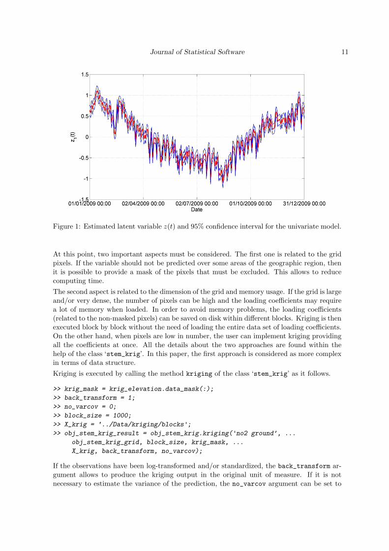
The estimate of the latent temporal variable z(t) is stored in the stem_kalmansmoother_resultobject which is a property of the stem_EM_result object. The graph of Figure 1 showsthe estimated temporal variable and it has been obtained calling the method plot of class‘stem_kalmansmoother_result’.

The estimated model is eventually used to map the NO2 concentration over the geographicregion following the kriging approach. Since the loading coefficients of this case study consistof a set of covariates, the same covariates must be available for the entire region as a regulargrid with the proper spatial resolution.

The first step toward mapping is to create the obj_stem_krig object of class ‘stem_krig’ inthe following way.

>> obj_stem_krig = stem_krig(obj_stem_model);

Since the kriging output is evaluated over a regular grid, the obj_stem_krig_grid object ofclass ‘stem_grid’ is created as follows.

>> load ../Data/kriging/krig_elevation_005;

>> krig_coordinates = [krig_elevation.lat(:), krig_elevation.lon(:)];

>> obj_stem_krig_grid = stem_grid(krig_coordinates, 'deg', 'regular', ...

'pixel', [80, 170], 'square', 0.05, 0.05);

As the grid is regular, the dimension of the grid must also be provided (80 rows and 170columns) as well as the shape of the pixels (square) and their dimension (0.05×0.05 degrees).


Figure 1: Estimated latent variable z(t) and 95% confidence interval for the univariate model.

At this point, two important aspects must be considered. The first one is related to the gridpixels. If the variable should not be predicted over some areas of the geographic region, thenit is possible to provide a mask of the pixels that must be excluded. This allows to reducecomputing time.

The second aspect is related to the dimension of the grid and memory usage. If the grid is largeand/or very dense, the number of pixels can be high and the loading coefficients may requirea lot of memory when loaded. In order to avoid memory problems, the loading coefficients(related to the non-masked pixels) can be saved on disk within different blocks. Kriging is thenexecuted block by block without the need of loading the entire data set of loading coefficients.On the other hand, when pixels are low in number, the user can implement kriging providingall the coefficients at once. All the details about the two approaches are found within thehelp of the class ‘stem_krig’. In this paper, the first approach is considered as more complexin terms of data structure.

Kriging is executed by calling the method kriging of the class ‘stem_krig’ as it follows.

>> krig_mask = krig_elevation.data_mask(:);

>> back_transform = 1;

>> no_varcov = 0;

>> block_size = 1000;

>> X_krig = '../Data/kriging/blocks';

>> obj_stem_krig_result = obj_stem_krig.kriging('no2 ground', ...

obj_stem_krig_grid, block_size, krig_mask, ...

X_krig, back_transform, no_varcov);

If the observations have been log-transformed and/or standardized, the back_transform ar-gument allows to produce the kriging output in the original unit of measure. If it is notnecessary to estimate the variance of the prediction, the no_varcov argument can be set to


1 saving computing time. Finally, note that the directory where the blocks are stored isprovided as well as the size (number of grid pixels) of each block.

The kriging result is saved in the obj_stem_krig_result object and the plot method canbe used to display the result on a map. For example, the estimated NO2 concentration andthe respective standard deviation for April 10, 2009 are depicted in Figure 2. Note that,since w(s, t) and xland(s) are interacted, the spatial pattern of the standard deviation doesnot reflect the monitoring network, that is, the standard deviation is not necessarily lowernear the monitoring stations.

5. Multivariate model

In order to demonstrate the multivariate capabilities of D-STEM, a simple bivariate case isintroduced. A more complex case study with three variables can be found in Finazzi et al.(2013).

In addition to the NO2 data of the previous section, measurements of particulate mattersconcentration PM2.5 coming from n2 = 44 monitoring stations over the same geographicregion are considered. Note that only a subset of the PM2.5 measurements are co-located tothe NO2 measurements. D-STEM, however, allows for fully or partially heterotopic networks.In this way, the spatial information of the more dense NO2 monitoring network may be usedto improve PM2.5 mapping.

The response variable is now y(s, t) = (yNO2(s, t), yPM2.5(s, t))> and the model in Equation 1is extended by introducing a bivariate temporal component z(t) and a bivariate space-timecomponent w(s, t) modeled through an LCM. The same covariates of the previous section areconsidered for both NO2 and PM2.5.


Multivariate models are tackled considering the following straightforward extension of themodel in Equation 2:

y(s, t) = µ(s, t) + ω(s, t) + ε(s, t), (6)

which unifies the modeling approaches developed in Zhang (2007), Fasso and Finazzi (2011)and Finazzi et al. (2013).

In particular, extending fixed and random effect models of Equations 3 and 4, we haveµ(s, t) = Xβ(s, t)β and

ω(s, t) =

c∑j=1

αj � xj(s, t)�wj(s, t) + Xz(s, t)z(t), (7)

where the symbol � represents the element by element or Hadamard product; moreovery(s, t), αj , xj(s, t), wj(s, t), j = 1, . . . , c and ε(s, t) are q × 1 vectors, while

Xβ(s, t) = blockdiag(xβ,1(s, t), . . . ,xβ,q(s, t)),Xz(s, t) = blockdiag(xz,1(s, t), . . . ,xz,p(s, t)),

where blockdiag is the block diagonal building operator. The vectors of loading coefficientsxβ,i(s, t) have dimensions 1 × bi for i = 1, . . . , q while the vectors xz,k(s, t) have dimensions1× ak for k = 1, . . . , p.


Figure 2: Estimated NO2 concentration [µg ·m−3] below 800 m of elevation (top) and stan-dard deviation (bottom) for April 10, 2009 over Northern Italy using the univariate model.Monitoring stations are depicted by the ‘+’ symbol.

In Equation 7, each multivariate spatial latent variable wj(s, t), for each fixed t, is modeledas a LCM with the following spatial variance-covariance matrix functions

Γj(‖s− s′‖) = Vjρ(‖s− s′‖; θj , ν), (8)

where Vj is a valid q×q correlation matrix and j = 1, . . . , c. On the other hand, the elementsof ε(s, t) are independent and normally distributed with variances σ2i , i = 1, . . . , q. It follows


that the parameter set for the model in Equation 6 is

ψ = {β,σ2,α,θ,v,G,vη},

where σ2 = (σ21, . . . , σ2q )>, α is the cq× 1 dimensional vector obtained by stacking α1, . . . ,αc

and v is the cq(q − 1)/2 × 1 dimensional vector obtained by stacking the unique and nondiagonal elements of V1, . . . ,Vc.


This paragraph describes the relevant lines of code of the demo_section5.m script. Thescript can be executed choosing option number two from the dstem_demo.m script. Sincedemo_section4.m of Section 4 and demo_section5.m are similar, only the differences inducedby the multivariate setting are detailed here.

The additional data related to the PM2.5 variable are loaded into the temporary structureground in the following way.

>> load ../Data/pm25_ground.mat

>> ground.Y{2} = pm25_ground.data;

>> ground.Y_name{2} = 'pm2.5 ground';

>> n2 = size(ground.Y{2}, 1);

Note that the second cell of the cell arrays Y and Y_name is used. The same strategy is followedfor X_beta, X_beta_name and so further. The coordinates of each variable must be providedseparately and added to the obj_stem_gridlist_p object as follows.

>> ground.coordinates{1} = [no2_ground.lat, no2_ground.lon];

>> ground.coordinates{2} = [pm25_ground.lat, pm25_ground.lon];

>> obj_stem_grid1 = stem_grid(ground.coordinates{1}, 'deg', 'sparse', ...

'point');

>> obj_stem_grid2 = stem_grid(ground.coordinates{2}, 'deg', 'sparse', ...

'point');

>> obj_stem_gridlist_p.add(obj_stem_grid1);

>> obj_stem_gridlist_p.add(obj_stem_grid2);

As in Section 4.2, the suffix “_p” refers to ground data because it is necessary to differentiatethen from the remote data of Section 6. Now, the obj_stem_par object is created in thefollowing way.

>> flag_time_diagonal = 0;

>> obj_stem_par = stem_par(obj_stem_data, 'exponential', [], ...

flag_time_diagonal);

Here, z(t) is bivariate (p = 2) and the flag_time_diagonal flag is introduced and used tospecify if the matrices G and Ση are diagonal or not. The following lines of code describethe initialization of the model parameters for the bivariate case.

>> obj_stem_par.beta = obj_stem_model.get_beta0();

>> obj_stem_par.alpha_p = [0.6 0.6]';


>> obj_stem_par.theta_p = 100;

>> obj_stem_par.v_p = [1 0.6; 0.6 1];

>> obj_stem_par.sigma_eta = diag([0.2 0.2]);

>> obj_stem_par.G = diag([0.8 0.8]);

>> obj_stem_par.sigma_eps = diag([0.3 0.3]);


Model estimation is thus obtained as in the previous section and it gives the following results.

********************************


********************************





'wind speed' '-0.174' '0.004'

'elevation' '-0.285' '0.008'

'sunday' '-0.103' '0.007'

* Beta coefficients related to the point variable pm2.5 ground


'wind speed' '-0.150' '0.007'

'elevation' '-0.203' '0.009'

'sunday' '-0.012' '0.013'



'no2 ground' '0.394' '0.002'

'pm2.5 ground' '0.322' '0.004'


* alpha_p elements:

[] 'elevation'

'no2 ground' '+0.603 (Std 0.005)'

[] 'elevation'

'pm2.5 ground' '+0.341 (Std 0.009)'

* theta_p elements:


'1st' '37.08' '0.95'



[] 'no2 ground' 'pm2.5 ground'

'no2 ground' '+1.00' '+0.70 (Std 0.02)'

'pm2.5 ground' '+0.70 (Std 0.02)' '+1.00'



'no2 ground' '+1.00 (Std 0.03)' '-0.05 (Std 0.02)'

'pm2.5 ground ' '+0.29 (Std 0.07)' '+0.72 (Std 0.05)'

* Sigma_eta matrix:


'no2 ground' '+0.03 (Std 0.01)' '+0.03 (Std 0.01)'

'pm2.5 ground' '+0.03 (Std 0.01)' '+0.10 (Std 0.01)'

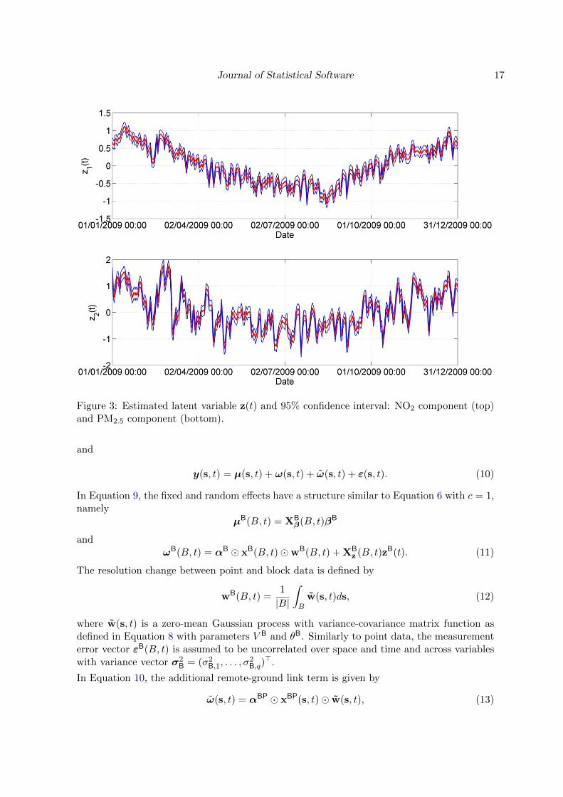
Figure 3 shows the components of the estimated z(t) related to both the variables. The graphsare obtained by calling the method plot of the class ‘stem_kalmansmoother_result’. Dailyconcentration maps of both variables can be obtained as in the previous section.

6. Data fusion model

In order to demonstrate the data fusion capability of D-STEM, the case study of the previoussection is extended by introducing remote sensing observations covering the same geographicregion. In particular, the tropospheric column density of NO2 (see Fasso and Finazzi 2013)and the so called aerosol optical thickness (AOT), which is known to be related to the groundlevel concentration of PM2.5 (Wang and Christopher 2003), are considered. The data areprovided as daily block averages over a regular grid with spatial resolution 1/4◦ that coversthe entire globe.

Remote sensing data may represent a valuable data source for estimating the ground levelvariables after statistical calibration based on the available ground level data. In doing this, achange of support problem (COSP) must be solved (Gotway and Young 2002). Depending onthe aim of the data analysis, the COSP can also be considered as a data fusion or downscalingproblem. Applications are not restricted to air quality remote sensing but include the case ofphysical model outputs and the case of environmental areal data in general.

The next paragraph discusses a general data fusion model suitable to jointly model groundlevel and remote sensing data solving the COSP.


The above remote sensing data can be considered a special case of block or pixel data whichare denoted here by yB(B, t), where B ⊂ D is the generic grid pixel. With this notation, themodel of Equation 6 is extended by introducing a new equation for remote sensing data anda downscaling link term into the ground data equation as follows:

yB(B, t) = µB(B, t) + ωB(B, t) + εB(B, t) (9)


Figure 3: Estimated latent variable z(t) and 95% confidence interval: NO2 component (top)and PM2.5 component (bottom).

and

y(s, t) = µ(s, t) + ω(s, t) + ω(s, t) + ε(s, t). (10)

In Equation 9, the fixed and random effects have a structure similar to Equation 6 with c = 1,namely

µB(B, t) = XBβ(B, t)βB

andωB(B, t) = αB � xB(B, t)�wB(B, t) + XB

z (B, t)zB(t). (11)

The resolution change between point and block data is defined by

wB(B, t) =1

|B|

∫B

w(s, t)ds, (12)

where w(s, t) is a zero-mean Gaussian process with variance-covariance matrix function asdefined in Equation 8 with parameters V B and θB. Similarly to point data, the measurementerror vector εB(B, t) is assumed to be uncorrelated over space and time and across variableswith variance vector σ2

B = (σ2B,1, . . . , σ2B,q)>.

In Equation 10, the additional remote-ground link term is given by

ω(s, t) = αBP � xBP(s, t)� w(s, t), (13)


where, the parameter vector αBP gives the intensity of the correlation between pixel and pointvariables, which can be modeled by the q × 1 vector of loading coefficients xBP(s, t).

Note that zB(t) is an additional Markovian component as the temporal dynamics may differbeween remote and ground data.

The parameter set for the data fusion model is

ψ = {β,βB,σ2,σ2B,α,α

BP,αB, θ,v, θB,vB,G,vη},

where vB is the q(q−1)/2×1 dimensional vector obtained by stacking the unique, non-diagonalelements of VB.

In many environmental applications, the grid of pixels is regular (all the pixels have the sameshape and dimension), the pixels are small compared to the geographic region and the processw(s, t) is smooth. In this case the approximations wB(B, t) ' w(s∗, t) and w(s, t) ' w(s∗, t),where s∗ is the center of B, are reasonable. D-STEM implements these approximationsavoiding the time-consuming computation of the integral in Equation 12 for each pixel Band each iteration of the EM algorithm. Possible errors induced by this approximation arecovered by εB(B, t).

The model in Equations 9 and 10 is similar to the Gaussian Markov random field smootheddownscaler developed in Berrocal, Gelfand, and Holland (2012), with the main difference thatD-STEM handles multivariate data and use Gaussian processes instead of Gaussian Markovrandom fields. In fact Gaussian processes, thanks to the EM algorithm, are more suitable forhandling extensive missing data which often arise in remote sensing.


This paragraph describes the demo_section6.m script which can be executed choosing optionnumber three from the dstem_demo.m script. Only the code related to the pixel variables andthe downscaler are discussed here, the reader being referred to the previous Section 5.2.

A simple version of the model in Equation 9 is considered here. In particular, remote sensingdata are described by the equation

yB(B, t) = αB �wB(B, t) + εB(B, t), (14)

and, similarly, xBP(s, t) = 1 is used in Equation 13. Hence a constant vector is added to thetemporary data structure ground of Section 5.2 as follows.

>> ground.X_bp{1} = ones(n1, 1);

>> ground.X_bp_name{1} = {'constant'};

>> ground.X_bp{2} = ones(n2, 1);

>> ground.X_bp_name{2} = {'constant'};

The observations related to the pixel variables are loaded from disk as detailed in the followinglines of code.

>> load ../Data/no2_remote_025.mat

>> remote.Y{1} = no2_remote.data;

>> remote.Y_name{1} = 'no2 remote';


>> m1 = size(remote.Y{1}, 1);

>> load ../Data/aot_remote_025.mat

>> remote.Y{2} = aot_remote.data;

>> remote.Y_name{2} = 'aot remote';

>> m2 = size(remote.Y{2}, 1);

Note that an additional temporary data structure remote is used. Since the model in Equa-tion 14 does not consider loading coefficients for the pixel variables, the constant vectorxB(B, t) = 1 is provided in the following way.

>> remote.X_bp{1} = ones(m1, 1);

>> remote.X_bp_name{1} = {'constant'};

>> remote.X_bp{2} = ones(m2, 1);

>> remote.X_bp_name{2} = {'constant'};

A second object of class ‘stem_varset’ is then created.

>> obj_stem_varset_b = stem_varset(remote.Y, remote.Y_name, remote.X_bp, ...

remote.X_bp_name);

Following the same strategy, a second object of class ‘stem_gridlist’ is created and it isused as a collector for the objects of class ‘stem_grid’ related to the pixel variables.

>> obj_stem_gridlist_b = stem_gridlist();

>> remote.coordinates{1} = [no2_remote.lat(:), no2_remote.lon(:)];

>> remote.coordinates{2} = [aot_remote.lat(:), aot_remote.lon(:)];

>> obj_stem_grid1 = stem_grid(remote.coordinates{1}, 'deg', 'regular', ...

'pixel', size(no2_remote.lat), 'square', 0.25, 0.25);

>> obj_stem_grid2 = stem_grid(remote.coordinates{2}, 'deg', 'regular', ...

'pixel', size(aot_remote.lat), 'square', 0.25, 0.25);

>> obj_stem_gridlist_b.add(obj_stem_grid1);

>> obj_stem_gridlist_b.add(obj_stem_grid2);

When multiple pixel variables are considered, it is possible to decide whether wB(B, t) is cross-correlated or not. If not, then the spatial correlation function of each variable is parametrizedby its own parameter vector θBi , i = 1, . . . , q. The additional flag_pixel_correlated flag isthus introduced and it is used as input argument in the creation of the obj_stem_data andobj_stem_par objects.

>> flag_pixel_correlated = 0;

>> flag_time_diagonal = 0;

>> obj_stem_data = stem_data(obj_stem_varset_p, obj_stem_gridlist_p, ...

obj_stem_varset_b, obj_stem_gridlist_b, obj_stem_datestamp, ...

[], [], [], flag_pixel_correlated);

>> obj_stem_par = stem_par(obj_stem_data, 'exponential', ...

flag_time_diagonal);

>> obj_stem_model = stem_model(obj_stem_data,obj_stem_par);

The model parameters related to the pixel variables are initialized in the following way.


>> obj_stem_par.alpha_bp = [0.4 0.4 0.8 0.8]';

>> if flag_pixel_correlated

obj_stem_par.theta_b = 100;

obj_stem_par.v_b = [1 0.6; 0.6 1];

else

obj_stem_par.theta_b = [100 100]';

obj_stem_par.v_b = eye(2);

end

>> obj_stem_par.sigma_eps = diag([0.3 0.3 0.3 0.3]);


Note that, depending on the value of flag_pixel_correlated, the parameter structure isdifferent. Moreover, alpha_bp is a 2q × 1 vector that includes both αBP and αB whilesigma_eps is a 2q × 2q diagonal matrix, where 2q is the total number of variables.

Model estimation and kriging are performed using the same lines of code detailed in theprevious sections and the estimation result is the following.

********************************


********************************


* Observed data log-likelihood: 7572.506



'wind speed' '-0.169' '0.004'

'elevation' '-0.252' '0.006'

'sunday' '-0.092' '0.007'

* Beta coefficients related to the point variable pm2.5 ground


'wind speed' '-0.142' '0.008'

'elevation' '-0.229' '0.008'

'sunday' '-0.018' '0.014'



'no2 ground' '0.383' '0.002'

'pm2.5 ground' '0.272' '0.004'

'no2 remote' '0.024' '0.001'

'aot remote' '0.065' '0.003'

* alpha_bp elements


'no2 ground' '+0.121' '0.004'

'pm2.5 ground' '+0.314' '0.009'


'no2 remote' '+0.891' '0.008'

'aot remote' '+0.999' '0.015'

* Pixel data are NOT cross-correlated.

* Theta_b elements:

'Variable' 'Value [km]' 'Std [km]'

'no2 remote' '118.896' '2.610'

'aot remote' '156.490' '5.348'


* alpha_p elements:

[] 'elevation'

'no2 ground' '+0.555 (Std 0.005)'

[] 'elevation'

'pm2.5 ground' '+0.302 (Std 0.008)'

* theta_p elements:


'1st' '21.97' '0.62'



'no2 ground' '+1.00' '+0.71 (Std 0.03)'

'pm2.5 ground' '+0.71 (Std 0.03)' '+1.00'



'no2 ground' '+0.95 (Std 0.04)' '-0.01 (Std 0.03)'

'pm2.5 ground' '+0.37 (Std 0.08)' '+0.63 (Std 0.06)'

* Sigma_eta matrix:


'no2 ground' '+0.03 (Std 0.01)' '+0.03 (Std 0.01)'

'pm2.5 ground' '+0.03 (Std 0.01)' '+0.10 (Std 0.01)'

The first q elements of the vector alpha_bp express how well the latent variable wB(B, t),which describes the pixel observations, is also able to describe the respective point observations(net of the other model terms). When observations and loading coefficients are standardized, avalue close to zero implies poor correlation while a value close to one implies high correlation.In this case study the values are 0.121 and 0.314 for NO2 and PM2.5, respectively, whichcorrespond to low/mild correlations.

Pixel variables are considered as secondary information useful to improve the mapping of thepoint variables. For this reason, kriging is not provided for pixel variables. Nevertheless,the estimated pixel variables, namely wB(B, t), are obtained over the original grid as a by-


product of model estimation. The following lines of code are used to plot the observed pixelvariable NO2 and the estimated wB(B, t) which is stored in the property E_wb_y1 of thestem_EM_result object.

>> obj_stem_model.stem_data.plot('no2 remote', 'pixel', 25);

>> size = obj_stem_model.stem_data.stem_gridlist_b.grid{1}.grid_size;

>> E_wb_y1 = obj_stem_model.stem_EM_result.E_wb_y1(1:size(1) * size(2), 25);

>> coordinate = obj_stem_model.stem_data.stem_gridlist_b.grid{1}.coordinate;

>> lat = coordinate(:, 1);

>> lon = coordinate(:, 2);

>> lat = reshape(lat,size);

>> lon = reshape(lon,size);

>> E_wb_y1 = reshape(E_wb_y1, size);

>> stem_misc.plot_map(lat, lon, E_wb_y1, obj_stem_model.stem_data.shape, ...

'no2 remote estimated on 25-Jan-2009', 'Longitude', 'Latitude');

The resulting maps are displayed in Figure 4. The observed pixel data are characterized bylarge areas of missing data but the latent variable wB(B, t) allows to reconstruct the missingdata and to filter the observed data corrupted by noise. Moreover, since wB(B, t) is used tomodel both point data and pixel data, the reconstruction of the missing pixel data benefitsfrom the observed point data.

7. Large data sets handling

The statistical models that D-STEM implements are separable with respect to space andtime. If N is the total number of spatial locations where all the point variables are observedand T is the total number of time steps, then the largest variance-covariance matrix thatD-STEM handles is only N ×N . If pixel variables are also considered and the total numberof pixels where all the variables are observed is M , then the largest variance-covariance matrixis D×D, where D = max(N,M). In many applications, however, N and D can be large andboth computing time and memory usage can increase drastically. In the following paragraphs,three strategies that D-STEM provides for reducing computing time are discussed. Even ifthese strategies are intended for large data sets, in order to keep the computing time feasible,the same case studies of the previous sections are considered.

7.1. Tapering

The tapering approach consists of adopting a sparse variance-covariance matrix characterizedby a high percentage of zero elements (possibly higher than 90%). The idea behind tapering isthat spatial locations at great distance should not exhibit spatial correlation. Hence, taperingforces to zero the covariances of observations at distances higher than a threshold in such away that the positive definiteness of the variance-covariance matrix is preserved.

When the generic variance-covariance matrix A is used to solve matrix equations in theform Ax = b, the computing time is greatly reduced if A is sparse. The higher the matrixsparseness the lower the computing time. In order to model spatial correlation, however,the above mentioned threshold cannot be too low and there exists a trade-off between low


Figure 4: Observed remote sensing NO2 data (top) and reconstructed data (bottom).

computing time and good approximation of the latent Gaussian processes used to describethe spatial correlation.

In order to implement tapering, D-STEM applies the so called one-taper tapering of Kaufman,Schervish, and Nychka (2008) to each LCM component wj(s, t). To do this, in the spatialcorrelation matrix function of Equation 8, the Matern correlation function ρ is substituted by

ρ(∥∥s− s′

∥∥ ; θj , ν) · Φ(‖s− s′‖

φ

),

where Φ(‖s−s′‖φ

)is the compactly supported radial Wendland function (Wendland and Math-

ematik 1995), with φ the width of the radial function.

Although the asymptotic theory of Kaufman et al. (2008) is proven for the purely spatialunivariate case, T = 1 and q = 1, in light of the results of Ruiz-Medina and Porcu (2014),we conjecture here that it holds true also for the purely spatial multivariate case, T = 1 andq > 1, and, a fortiori, for the space-time case with large T . Note that, unlike the so calledtwo-tapers tapering of Kaufman et al. (2008), the one-taper may give a biased estimate of θ in


case the tapering range φ is small compared to the data correlation range. However, accordingto Kaufman et al. (2008), the two-tapers approach has a substantially heavier computationalburden while the one-taper approach gives better kriging performance, which is an importantaim of D-STEM.

The demo_section7_1.m script, which can be executed by choosing option number four fromthe dstem_demo.m script, implements the same case study of Section 6 with tapering enabled.In particular, tapering can be enabled by providing the width φ (expressed in kilometers) ofthe Wendland function to the constructor of the class ‘stem_gridlist’ as follows.

>> phi_p = 50;

>> obj_stem_gridlist_p = stem_gridlist(phi_p);

>> phi_b = 200;

>> obj_stem_gridlist_b = stem_gridlist(phi_b);

The width φ is a property of the grids as all the variance-covariance matrices are directlyderived from the distance matrices which, in order to reduce memory usage, are also createdas sparse matrices. Also note that φ can be different for point and pixel data.

The output of model estimation is similar to the output reported in Section 6 and only therelevant part is reported hereafter.

********************************


********************************

* Tapering is enabled.

Point data tapering: 50 km

Pixel data tapering: 200 km

* Observed data log-likelihood: 6182.198

* Theta_b elements:

'Variable' 'Value [km]' 'Std [km]'

'no2 remote' '242.369' ' 8.250'

'aot remote' '365.052' '34.033'


* theta_p elements:


'1st' '198.22' '80.21'

Looking at the estimation result, it can be noted that the estimated θ parameters, as wellas their standard deviations, are higher compared to those reported in Section 6. Moreover,the observed data log-likelihood is lower. The tapering approach, thus, reduces computingtime but may produce biased estimates of the θ parameters and/or estimates with a largeruncertainty. Finally, note that tapering is intended for large data sets. The case studiesdiscussed in this paper are based on medium-size data sets so that the actual computing timemay be higher when tapering is enabled. The same consideration applies to the two followingstrategies.


7.2. Computing load distribution

Thanks to the separability between space and time, most of the matrix algebra operationsat the basis of the EM algorithm only involve the data of a single time step. Moreover, eachtime step is independent from the previous and the next time steps. The Kalman filter itselfis implemented in such a way that some operations executed at time t are independent fromthe result of the operations at time t− 1.

If a cluster of computing nodes is available, then model estimation can be performed in adistributed manner. In particular, if n nodes are available and T ≥ n, then the data setis split into n temporal frames and distributed to the nodes on the basis of the node speed(evaluated at each EM iteration) and the number of missing data in each time frame. Indeed,time steps characterized by a high missing data rate imply faster computing.

The computing nodes can be any number of heterogeneous machines connected through alocal area network (LAN) and no additional parallel and/or distributed software libraries arerequired. All the nodes must be able to read and write to a common shared folder and eachnode must run at least one MATLAB process. One node, usually the fastest or the one withthe highest quantity of RAM, is designated to be the master while all the other nodes areconsidered slaves. The number of slaves can change during model estimation but the masternode must always run.

In order to estimate the model in a distributed manner, a script that calls the daemon.m

function must first be executed on each slave node possibly in batch mode. The functionrequires as input argument the path of the shared folder to use. The master runs the usualmain script but the name of the shared folder, as well as additional parameters, must be givenas properties of the obj_stem_EM_options object.

Choosing option number five from the dstem_demo.m script, the case study of Section 6 isreproduced and model estimation is carried out in distributed manner. To avoid the com-plication of setting up a distributed environment, the dstem_demo.m script starts a secondMATLAB process in which the demo_runslave script is executed and that, in turn, executesthe daemon.m script. The original MATLAB process executes the demo_section7_2.m scriptwhich differs from the demo_section6.m script with respect to the following lines of code.

>> exit_toll = 0.001;


>> path_distributed_computing = '../Distributed/';

>> timeout = 5;

>> obj_stem_EM_options = stem_EM_options(exit_toll, max_iterations, [], [], ...

[], [], path_distributed_computing, [], timeout);


The timeout input argument is the time in seconds that the master waits when listeningfor the slave nodes. It is worth knowing that the content of NFS shared folders on UNIXdistributed environments is not always updated in real time. If the user cannot change theupdating time of NFS folders, then the timeout input argument must be increased in orderto ensure that master and slaves can always read the files written in the shared folder.

The output of model estimation is equal to the output already reported and discussed inSection 6.


7.3. Observed data log-likelihood evaluation

By default, D-STEM compares the estimated parameters and the observed data log-likelihoodbetween two consecutive EM iterations. If the relative norm of the difference between theparameter vectors or between the log-likelihoods is lower than the tolerance specified by theproperty exit_toll of class ‘stem_EM_options’ (see Section 4.2), the EM algorithm stops.In the case of large data sets, computing the log-likelihood at each EM iteration is timeconsuming. In order to speed up model estimation, the evaluation of the log-likelihood canbe avoided and the exit condition is only based on the model parameters.

The demo_section7_3.m script, which can be executed choosing option number six from thedstem_demo.m script, implements the same case study as in Section 4 but model estimationis carried out without computing the observed data log-likelihood at each iteration.

The following lines of code describe how the obj_stem_EM_options object is created in orderto avoid the evaluation of the log-likelihood at each iteration.

>> exit_toll = 0.001;


>> compute_log = 0;

>> obj_stem_EM_options = stem_EM_options(exit_toll, max_iterations, ...

[], [], compute_log);


The output of the model estimation is similar to the output reported in Section 4 and onlythe relevant part is reported hereafter.

********************************


********************************




* theta_p elements:


'1st' '22.45' '0.63'

Due to the different exit condition, the model parameters estimated without computing thelog-likelihood at each iteration differ from those estimated in Section 4. In particular, the θparameter decreased from 31.42 to 22.45 km. Nonetheless, the observed data log-likelihood,evaluated after model estimation, is only slightly higher (−13797.357 vs. −13889.064). Thisis due to the fact that, using a non-large data set as in this case study, the θ parameter ofEquation 5 is poorly identifiable and it monotonically changes from one iteration to the nexteven if the observed data log-likelihood does not change significantly.

Although the computing time of each iteration is reduced, thus, a possible drawback is thatthe total number of iterations required to estimate the model might be higher. The user


should be careful when adopting this strategy as, if poor identifiability of θ is not detected,the EM algorithm might not converge or it might take more iterations than necessary. Inthe above example, the EM algorithm takes 78 iterations to converge with respect to the 32iterations required when the log-likelihood is evaluated at each iteration. Again, this strategyto reduce computing time is intended for large data sets.

8. Conclusions

In this paper, the use of D-STEM has been illustrated for three different case studies involvinga univariate model, a bivariate model and a data fusion model. The model at the basis ofD-STEM is general enough to accommodate many environmental data sets, nonetheless, bothmodel and software can be extended with respect to many aspects. From the modeling pointof view, additional spatial correlation functions could be introduced as well as more flexible“coregionalization models” (Apanasovich and Genton 2010; Gneiting, Kleiber, and Schlather2010). Moreover, Markov random fields could be introduced in order to model pixel data.Indeed, Gaussian random fields easily handle data sets with extensive missing data but theyare more computationally expensive even under tapering. Finally, it could be useful to extendthe model to accommodate for time-varying grids and irregularly spaced sampling times.

Regardint the software side, some time consuming procedures such as the estimation of thevariance-covariance matrix of the model parameters and kriging could also be implemented ina distributed manner. Furthermore, the handling of the model parameters could be improvedby introducing constraints on the parameter vectors and matrices, widening the range ofmodels that can be estimated.

D-STEM is constantly updated and improved and new versions are released on https://

code.google.com/p/d-stem/. Google Code runs a project hosting service that providesrevision control and an issue tracker. The users of D-STEM are welcome to notify bugs andto submit extensions or improvements of the code.

References

Apanasovich TV, Genton MG (2010). “Cross-Covariance Functions for Multivariate RandomFields Based on Latent Dimensions.” Biometrika, 97(1), 15–30.

Bakar KS, Sahu SK (2014a). “spTimer: Spatio-Temporal Bayesian Modeling Using R.” Jour-nal of Statistical Software. Forthcoming.

Bakar KS, Sahu SK (2014b). spTimer: Spatio-Temporal Bayesian Modelling Using R.R package version 1.0-3, URL http://CRAN.R-project.org/package=spTimer.

Berrocal VJ, Gelfand AE, Holland DM (2012). “Space-Time Data Fusion Under Error inComputer Model Output: An Application to Modeling Air Quality.” Biometrics, 68(3),837–848.

Cameletti M (2012). Stem: Spatio-Temporal Models in R. R package version 1.0, URLhttp://CRAN.R-project.org/package=Stem.



http://CRAN.R-project.org/package=spTimer

http://CRAN.R-project.org/package=Stem


Cameletti M, Lindgren F, Simpson D, Rue H (2013). “Spatio-Temporal Modeling of Partic-ulate Matter Concentration through the SPDE Approach.” AStA Advances in StatisticalAnalysis, 97(2), 109–131.

Cressie NAC, Wikle CK (2011). Statistics for Spatio-Temporal Data. Wiley Series in Proba-bility and Statistics. John Wiley & Sons.

Fasso A (2013). “Statistical Assessment of Air Quality Interventions.” Stochastic Environ-mental Research and Risk Assessment, 27(7), 1651–1660.

Fasso A, Finazzi F (2011). “Maximum Likelihood Estimation of the Dynamic Coregionaliza-tion Model with Heterotopic Data.” Environmetrics, 22(6), 735–748.

Fasso A, Finazzi F (2013). “A Varying Coefficients Space-Time Model for Ground and SatelliteAir Quality Data over Europe.” Statistica & Applicazioni, Special Online Issue, 45–56.

Finazzi F, Scott EM, Fasso A (2013). “A Model-Based Framework for Air Quality Indices andPopulation Risk Evaluation, with an Application to the Analysis of Scottish Air QualityData.” Journal of the Royal Statistical Society C, 62(2), 287–308.

Gneiting T, Kleiber W, Schlather M (2010). “Matern Cross-Covariance Functions for Multi-variate Random Fields.” Journal of the American Statistical Association, 105(491), 1167–1177.

Gotway CA, Young LJ (2002). “Combining Incompatible Spatial Data.” Journal of theAmerican Statistical Association, 97(458), 632–648.

Katzfuss M, Cressie N (2011). “Spatio-Temporal Smoothing and EM Estimation for MassiveRemote-Sensing Data Sets.” Journal of Time Series Analysis, 32(4), 430–446.

Kaufman CG, Schervish MJ, Nychka DW (2008). “Covariance Tapering for Likelihood-BasedEstimation in Large Spatial Data Sets.” Journal of the American Statistical Association,103(484), 1545–1555.

Pebesma E, Gaeler B (2013). gstat: Spatial and Spatio-Temporal Geostatistical Modelling,Prediction and Simulation. R package version 1.0-17, URL http://CRAN.R-project.org/

package=gstat.

R Core Team (2014). R: A Language and Environment for Statistical Computing. R Founda-tion for Statistical Computing, Vienna, Austria. URL http://www.R-project.org/.

Rue H, Martino S, Lindgren F, Simpson D, Riebler A, Krainski ET (2014). INLA: Func-tions which Allow to Perform Full Bayesian Analysis of Latent Gaussian Models us-ing Integrated Nested Laplace Approximaxion. R package version 0.0-1404466487, URLhttp://www.R-INLA.org/.

Ruiz-Medina MD, Porcu E (2014). “Equivalence of Gaussian Measures of Multivari-ate Random Fields.” Stochastic Environmental Research and Risk Assessment. doi:

10.1007/s00477-014-0926-z. Forthcoming.

The MathWorks, Inc (2010). MATLAB, Statistics Toolbox, Optimization Toolbox and Map-ping Toolbox Release 2010b. Natick, Massachusetts, United States. URL http://www.

mathworks.com/.

http://CRAN.R-project.org/package=gstat

http://CRAN.R-project.org/package=gstat

http://www.R-project.org/

http://www.R-INLA.org/

http://dx.doi.org/10.1007/s00477-014-0926-z

http://dx.doi.org/10.1007/s00477-014-0926-z

http://www.mathworks.com/

http://www.mathworks.com/


Wang J, Christopher SA (2003). “Intercomparison Between Satellite-Derived Aerosol OpticalThickness and PM2.5 Mass: Implications for Air Quality Studies.” Geophysical ResearchLetters, 30(21), 2095.

Wendland H, Mathematik A (1995). “Piecewise Polynomial, Positive Definite and CompactlySupported Radial Functions of Minimal Degree.” Advances in Computational Mathematics,4(1), 389–396.

Zhang H (2007). “Maximum-Likelihood Estimation for Multivariate Spatial Linear Coregion-alization Models.” Environmetrics, 18(2), 125–139.

Affiliation:

Francesco FinazziDepartment of Management, Economics and Quantitative MethodsUniversity of Bergamovia dei Caniana, 224127 Bergamo (BG), ItalyE-mail: [email protected]: http://www.unibg.it/pers/?francesco.finazzi

Alessandro FassoDepartment of EngineeringUniversity of Bergamoviale Marconi, 524044 Dalmine (BG), ItalyE-mail: [email protected]: http://www.unibg.it/pers/?alessandro.fasso

Journal of Statistical Software http://www.jstatsoft.org/

published by the American Statistical Association http://www.amstat.org/

Volume 62, Issue 6 Submitted: 2013-08-05December 2014 Accepted: 2014-07-11

mailto:[email protected]

http://www.unibg.it/pers/?francesco.finazzi

mailto:[email protected]

http://www.unibg.it/pers/?alessandro.fasso

http://www.jstatsoft.org/

http://www.amstat.org/

Documents

D-STEM: A Software for the Analysis and Mapping …2 D-STEM: Analysis and Mapping of Environmental Space-Time Variables detailed in this paper by introducing three case studies of