Accepted by the Astronomical Journal, March 24, 2009Preprint typeset using LATEX style emulateapj v. 03/07/07

ORBITS AND MASSES OF THE SATELLITES OF THEDWARF PLANET HAUMEA = 2003 EL61

D. Ragozzine and M. E. BrownDivision of Geological and Planetary Sciences, California Institute of Technology, Pasadena, CA 91125

Accepted by the Astronomical Journal, March 24, 2009

ABSTRACT

Using precise relative astrometry from the Hubble Space Telescope and the W. M. Keck Telescope,we have determined the orbits and masses of the two dynamically interacting satellites of the dwarfplanet (136108) Haumea, formerly 2003 EL61. The orbital parameters of Hi’iaka, the outer, brightersatellite, match well the previously derived orbit. On timescales longer than a few weeks, no Keplerianorbit is sufficient to describe the motion of the inner, fainter satellite Namaka. Using a fully-interactingthree point-mass model, we have recovered the orbital parameters of both orbits and the mass ofHaumea and Hi’iaka; Namaka’s mass is marginally detected. The data are not sufficient to uniquelydetermine the gravitational quadrupole of the non-spherical primary (described by J2). The nearlyco-planar nature of the satellites, as well as an inferred density similar to water ice, strengthen thehypothesis that Haumea experienced a giant collision billions of years ago. The excited eccentricitiesand mutual inclination point to an intriguing tidal history of significant semi-major axis evolutionthrough satellite mean-motion resonances. The orbital solution indicates that Namaka and Haumeaare currently undergoing mutual events and that the mutual event season will last for the next severalyears.

Subject headings: comets: general — Kuiper Belt — minor planets — solar system: formation

1. INTRODUCTION

The dwarf planet (136108) Haumea, formerly2003 EL61, and about 3/4 of other large Kuiper beltobjects (KBOs) have at least one small close-in satel-lite (Weaver et al. 2006; Brown et al. 2006; Brown &Suer 2007). All of these larger KBOs are part of the ex-cited Kuiper belt, where the detectable binary fractionamong smaller KBOs is much lower, only a few percent(Stephens & Noll 2006). In contrast, the cold classicalpopulation (inclinations . 5) has no large KBOs (Lev-ison & Stern 2001; Brown 2008), but prevalent widelyseparated binaries with nearly equal masses (Noll et al.2008). The differences between the types and frequencyof Kuiper belt binaries may point to different binary for-mation mechanisms. Small satellites of large KBOs ap-pear to be formed by collision, as proposed for the Plutosystem (Canup 2005; Stern et al. 2006), Eris and Dysno-mia (Brown & Schaller 2007, but see Greenberg & Barnes2008), and Haumea (Barkume et al. 2006; Brown et al.2007; Fraser & Brown 2009), but smaller KBO binarieshave more angular momentum than can be generatedin typical impacts and are apparently formed by someother mechanism (e.g., Weidenschilling 2002; Goldreichet al. 2002; Funato et al. 2004; Astakhov et al. 2005;Nesvorny 2008). Both mechanisms of binary formationrequire higher number densities than present in the cur-rent Kuiper belt, as modeled explicitly for the Haumeacollision by Levison et al. (2008).

The collisional origin of Haumea’s two satellites — theouter, brighter satellite Hi’iaka (S1) and the inner, faintersatellite Namaka (S2) — is inferred from several relatedobservations. Haumea has a moderate-amplitude light-curve and the shortest rotation period (3.9155 hours)among known objects of its size (Rabinowitz et al. 2006).

Electronic address: darin@gps.caltech.edu

The rapid rotation requires a large spin angular momen-tum, as imparted by a large oblique impact. Using themass of Haumea derived by the orbit of Hi’iaka (Brownet al. 2005, hereafter B05), assuming Haumea’s rotationaxis is nearly perpendicular to the line-of-sight (like thesatellites’ orbits), and assuming the shape is that of aJacobi ellipsoid (a homogeneous fluid), the photometriclight curve can be used to determine the size, shape,albedo, and density of Haumea (Rabinowitz et al. 2006;Lacerda & Jewitt 2007, but see Holsapple 2007). It isestimated that Haumea is a tri-axial ellipsoid with ap-proximate semi-axes of 500 x 750 x 1000 km with a highalbedo (0.73) and density (2.6 g/cm3), as determined byRabinowitz et al. (2006). This size and albedo are con-sistent with Spitzer radiometry (Stansberry et al. 2008).The inferred density is near that of rock and higher thanall known KBOs implying an atypically small ice frac-tion.

Haumea is also the progenitor of the only known col-lisional family in the Kuiper belt (Brown et al. 2007).It seems that the collision that imparted the spin an-gular momentum also fragmented and removed the icymantle of the proto-Haumea (thus increasing its density)and ejected these fragments into their own heliocentricorbits. The Haumea family members are uniquely iden-tified by deep water ice spectra and optically neutralcolor (Brown et al. 2007), flat phase curves (Rabinowitzet al. 2008), and tight dynamical clustering (Ragozzine &Brown 2007). The dynamical clustering is so significantthat Ragozzine & Brown (2007) were able to correctlypredict that 2003 UZ117 and 2005 CB79 would have deepwater ice spectra characteristic of the Haumea family, asverified by Schaller & Brown (2008). The distribution oforbital elements matches the unique signature of a col-lisional family, when resonance diffusion (e.g., Nesvorny& Roig 2001) is taken into account. Using this resonance

2 Ragozzine & Brown

diffusion as a chronometer, Ragozzine & Brown (2007)find that the Haumea family-forming collision occurredat least 1 GYr ago and is probably primordial. This isconsistent with the results of Levison et al. (2008), whoconclude that the Haumea collision is only probable be-tween two scattered-disk objects in the early outer solarsystem when the number densities were much higher.

In this work, we have derived the orbits and massesof Haumea, Hi’iaka, and Namaka. In Section 2, we de-scribe the observations used to determine precise relativeastrometry. The orbit-fitting techniques and results aregiven in Section 3. Section 4 discusses the implicationsof the derived orbits on the past and present state of thesystem. We conclude the discussion of this interestingsystem in Section 5.

2. OBSERVATIONS AND DATA REDUCTION

Our data analysis uses observations from various cam-eras on the Hubble Space Telescope (HST) and theNIRC2 camera with Laser Guide Star Adaptive Objectsat the W. M. Keck Observatory. These observations areprocessed in different ways; here we describe the generaltechnique and below we discuss the individual observa-tions. Even on our relatively faint targets (V ≈ 21, 22),these powerful telescopes can achieve relative astrome-try with a precision of a few milliarcseconds. The Ju-lian Date of observation, the relative astrometric distanceon-the-sky, and the estimated astrometric errors are re-ported in Table 1.

Observations from Keck are reduced as in B05. Knownbad pixels were interpolated over and each image di-vided by a median flat-field. The images were then pair-wise subtracted (from images taken with the same fil-ter). The astrometric centroid of each of the visible ob-jects is determined by fitting two-dimensional Gaussians.Converting image distance to on-the-sky astrometric dis-tance is achieved using the recently derived pixel scaleof Ghez et al. (2008), who calibrate the absolute as-trometry of the NIRC2 camera and find a plate scaleof 0.009963”/pixel (compared to the previously assumedvalue of 0.009942”/pixel) and an additional rotation of0.13 compared with the rotation information providedin image headers. Ghez et al. (2008) and He lminiak &Konacki (2008) find that the plate-scale and rotation arestable over the timescale of our observations. Error barsare determined from the scatter of the measured dis-tances from each individual image; typical integrationtimes were about 1 minute. When the inner satellite isnot detected in individual images, but can be seen inthe stacked image, then the position is taken from thestacked image, after individually rotating, and the er-ror bars are simply scaled to the error bars of the outersatellite by multiplying by the square root of the ratioof signal/noise (∼5). The minute warping of the NIRC2fields1 is much smaller than the quoted error bars.

HST benefits from a known and stable PSF and well-calibrated relative astrometry. This allows for precisemeasurements, even when the satellites are quite closeto Haumea. For each of the HST observations, modelPSFs were generated using Tiny Tim2. The model PSFs

1 See the NIRC2 Astrometry page at http://www2.keck.hawaii.edu/inst/nirc2/forReDoc/post observing/dewarp/.

2 http://www.stsci.edu/software/tinytim/tinytim.html.

assumed solar colors, as appropriate for Haumea and itssatellites, and were otherwise processed according to thedetails given in The Tiny Tim User’s Guide. All threePSFs were then fitted simultaneously to minimize χ2,with errors taken from photon and sky noise added inquadrature. Bad pixels and cosmic rays were identi-fied by hand and masked out of the χ2 determination.The distortion correction of Anderson & King (2003) forWFPC2 is smaller than our error bars for our narrowangle astrometry and was not included. Relative on-the-sky positions were calculated using the xyad routine ofthe IDL Astro Library, which utilizes astrometry infor-mation from the image headers.

The acquisition and analysis of the satellite imagestaken in 2005 at Keck are described in B05. However,there is a sign error in the R. A. Offsets listed in Table1 of 2005; the values listed are actually the on-the-skydeviations (as visible from their Figure 1). Despite thistypographical error, the fit of B05 was carried out cor-rectly. The observed locations and estimated errors ofthe inner satellite are given in Brown et al. (2006). Theastrometric positions reported in Table 1 are slightly dif-ferent based on a reanalysis of some of the data as well asa new plate scale and rotation, discussed above. Basedon our orbital solution and a reinvestigation of the im-ages, we have determined that the May 28, 2005 obser-vation of Namaka reported in Brown et al. (2006) wasspurious; residual long-lived speckles from the adaptiveoptics correction are often difficult to distinguish fromfaint close-in satellites.

In 2006, HST observed Haumea with the High Resolu-tion Camera of the Advanced Camera for Surveys (Pro-gram 10545). Two five minute integrations were takenat the beginning and end of a single orbit. The raw im-ages were used for fitting, requiring distorted PSFs anddistortion-corrected astrometry. The astrometric accu-racy of ACS is estimated to be ∼0.1 pixels to which weadd the photon noise error in the positions of the threeobjects. The high precision of ACS allows for motion tobe detected between these two exposures, so these errorsare not based on the scatter of multiple measurementsas with all the other measurements.

At the beginning of February 2007, Hubble observedHaumea for 5 orbits, obtaining highly accurate positionsfor both satellites (Program 10860). The motion of thesatellites from orbit to orbit is easily detected, and mo-tion during a single orbit can even be significant, sowe subdivided these images into 10 separate “observa-tions”. The timing of the observations were chosen tohave a star in the field of view, from which the TinyTim PSF parameters are modeled in manner describedin Brown & Trujillo (2004). The observations do nottrack Haumea, but are fixed on the star to get the bestPSF which is then appropriately smeared for the mo-tion of the objects. Even though these observations weretaken with the Wide Field Planetary Camera — the ACSHigh-Resolution Camera failed only a week earlier — thePSF fitting works excellently and provides precise po-sitions. Astrometric errors for these observations weredetermined from the observed scatter in positions aftersubtracting the best fit quadratic trend to the data, sothat observed orbital motion is not included in the er-ror estimate. We note here that combined deep stacksof these images revealed no additional outer satellites

Satellites of Haumea 3

TABLE 1Observed Astrometric Positions for the Haumea System

Julian Date Date Telescope Camera ∆xH ∆yH σ∆xHσ∆yH

∆xN ∆yN σ∆xNσ∆yN

arcsec arcsec arcsec arcsec

2453397.162 2005 Jan 26 Keck NIRC2 0.03506 -0.63055 0.01394 0.01394 · · · · · · · · · · · ·

2453431.009 2005 Mar 1 Keck NIRC2 0.29390 -1.00626 0.02291 0.02291 0.00992 0.52801 0.02986 0.029862453433.984 2005 Mar 4 Keck NIRC2 0.33974 -1.26530 0.01992 0.01992 · · · · · · · · · · · ·

2453518.816 2005 May 28 Keck NIRC2 -0.06226 0.60575 0.00996 0.00996 · · · · · · · · · · · ·

2453551.810 2005 Jun 30 Keck NIRC2 -0.19727 0.52106 0.00498 0.00996 -0.03988 -0.65739 0.03978 0.039782453746.525 2006 Jan 11 HST ACS/HRC -0.20637 0.30013 0.00256 0.00256 0.04134 -0.18746 0.00267 0.002672453746.554 2006 Jan 11 HST ACS/HRC -0.20832 0.30582 0.00257 0.00257 0.03867 -0.19174 0.00267 0.002672454138.287 2007 Feb 6 HST WFPC2 -0.21088 0.22019 0.00252 0.00197 -0.02627 -0.57004 0.00702 0.003512454138.304 2007 Feb 6 HST WFPC2 -0.21132 0.22145 0.00095 0.00204 -0.03107 -0.56624 0.00210 0.007822454138.351 2007 Feb 6 HST WFPC2 -0.21515 0.23185 0.00301 0.00206 -0.03009 -0.55811 0.00527 0.005642454138.368 2007 Feb 6 HST WFPC2 -0.21402 0.23314 0.00192 0.00230 -0.03133 -0.56000 0.00482 0.006632454138.418 2007 Feb 6 HST WFPC2 -0.21705 0.24202 0.00103 0.00282 -0.03134 -0.54559 0.00385 0.003762454138.435 2007 Feb 6 HST WFPC2 -0.21449 0.24450 0.00323 0.00254 -0.02791 -0.54794 0.00571 0.005242454138.484 2007 Feb 6 HST WFPC2 -0.21818 0.25301 0.00153 0.00224 -0.02972 -0.53385 0.00797 0.013302454138.501 2007 Feb 7 HST WFPC2 -0.21807 0.25639 0.00310 0.00291 -0.03226 -0.53727 0.00531 0.004002454138.551 2007 Feb 7 HST WFPC2 -0.22173 0.26308 0.00146 0.00230 -0.03429 -0.53079 0.00497 0.005822454138.567 2007 Feb 7 HST WFPC2 -0.21978 0.26791 0.00202 0.00226 -0.03576 -0.52712 0.00270 0.004792454469.653 2008 Jan 4 HST WFPC2 0.23786 -1.27383 0.00404 0.00824 -0.02399 -0.28555 0.00670 0.008312454552.897 2008 Mar 27 Keck NIRC2 0.19974 -0.10941 0.00930 0.00956 · · · · · · · · · · · ·

2454556.929 2008 Mar 31 Keck NIRC2 0.32988 -0.77111 0.00455 0.00557 0.00439 -0.76848 0.01239 0.012802454556.948 2008 Mar 31 Keck NIRC2 0.33367 -0.77427 0.00890 0.00753 0.01363 -0.76500 0.01976 0.012522454556.964 2008 Mar 31 Keck NIRC2 0.33267 -0.77874 0.00676 0.00485 0.00576 -0.77375 0.01212 0.012832454557.004 2008 Mar 31 Keck NIRC2 0.33543 -0.78372 0.00404 0.00592 0.00854 -0.77313 0.01199 0.008972454557.020 2008 Mar 31 Keck NIRC2 0.33491 -0.78368 0.00374 0.00473 0.00075 -0.76974 0.00907 0.010152454557.039 2008 Mar 31 Keck NIRC2 0.33712 -0.78464 0.00740 0.00936 0.00988 -0.77084 0.01793 0.015432454557.058 2008 Mar 31 Keck NIRC2 0.33549 -0.78692 0.00868 0.00852 0.01533 -0.76117 0.00765 0.015712454557.074 2008 Mar 31 Keck NIRC2 0.33128 -0.78867 0.01431 0.01411 0.00645 -0.76297 0.01639 0.013902454557.091 2008 Mar 31 Keck NIRC2 0.33687 -0.79462 0.00803 0.00717 0.00708 -0.76986 0.01532 0.007872454593.726 2008 May 7 HST NICMOS -0.18297 1.08994 0.00354 0.00425 0.00243 -0.75878 0.00576 0.007612454600.192 2008 May 13 HST WFPC2 0.10847 0.17074 0.00508 0.00427 -0.02325 0.19934 0.00480 0.011612454601.990 2008 May 15 HST WFPC2 0.18374 -0.13041 0.00729 0.00504 -0.02293 0.50217 0.00618 0.006142454603.788 2008 May 17 HST WFPC2 0.24918 -0.43962 0.00207 0.00574 -0.01174 0.59613 0.00366 0.004852454605.788 2008 May 19 HST WFPC2 0.29818 -0.75412 0.00467 0.00966 0.00006 0.29915 0.00425 0.00613

Note. — Summary of observations of the astrometric positions of Hi’iaka (H) and Namaka (N) relative to Haumea. The difference in brightness(∼6) and orbital planes allow for a unique identification of each satellite without possibility of confusion. The method for obtaining the astrometricpositions and errors is described in Section 2 and Brown et al. (2005). On a few dates, the fainter Namaka was not detected because the observationswere not of sufficiently deep or Namaka was located within the PSF of Haumea. This data is shown graphically in Figure 2 and the residuals to thefit shown in Figure 3. For reasons described in the text, only the HST data is used to calculate the orbital parameters, which are shown in Table 2.

brighter than ∼0.25% fractional brightness at distancesout to about a tenth of the Hill sphere (i.e. about 0.1% ofthe volume where additional satellites would be stable).

In 2008, we observed Haumea with Keck NIRC2 onthe nights of March 28 and March 31. The observationson March 31 in H band lasted for about 5 hours undergood conditions, with clear detections of both satellitesin each image. These were processed as described above.Observations where Haumea had a large FWHM wereremoved; about 75% of the data was kept. As with theFebruary 2007 HST data, we divided the observationsinto 10 separate epochs and determined errors from scat-ter after subtracting a quadratic trend. The motion ofthe outer satellite is easily detected, but the inner satel-lite does not move (relative to Haumea) within the errorsbecause it is at southern elongation. The March 28 datawas not nearly as good as the March 31 data due to poorweather conditions and only the outer satellite is clearlydetected.

In early May 2008, HST observed Haumea using theNICMOS camera (Program 11169). These observationswere processed as described above, though a few imageswith obvious astrometric errors (due to the cosmic rayswhich riddle these images) were discarded. These are thesame observations discussed by Fraser & Brown (2009).

In mid-May 2008, we observed Haumea at five epochs

using the Wide Field Planetary Camera (WFPC2), overthe course of 8 days (Program 11518). Each of thesevisits consisted of four ∼10 minute exposures. Thesedata, along with an observation in January 2008, wereprocessed as described above. Although we expect thatsome of these cases may have marginally detected motionof the satellites between the four exposures, ignoring themotion only has the effect of slightly inflating the errorbars for these observations. Namaka was too close toHaumea (. 0.1”) to observe in the May 12, 2008 image,which is not used.

The derived on-the-sky relative astrometry for eachsatellite, along with the average Julian Date of the ob-servation and other information are summarized in Ta-ble 1. These are the astrometric data used for orbitfitting in this paper. In earlier attempts to determinethe orbit of Namaka, we also obtained other observa-tions. On the nights of April 20 and 21, 2006, we ob-served Haumea with the OSIRIS camera and LGSAO atKeck. Although OSIRIS is an integral-field spectrome-ter, our observations were taken in photometric mode. Inco-added images, both satellites were detected on bothnights. We also received queue-scheduled observationsof Haumea with the NIRI camera on Gemini and theLGSAO system Altair. In 2007, our Gemini program re-sulted in four good nights of data on April 9 and 13, May

4 Ragozzine & Brown

4, and June 5. In 2008, good observations were taken onApril 20, May 27, and May 28. In each of the Geminiimages, the brighter satellite is readily found, but thefainter satellite is often undetectable.

The accuracy of the plate scale and rotation requiredfor including OSIRIS and Gemini observations is un-known, so these data are not used for orbit determina-tion. We have, however, projected the orbits derived be-low to the positions of all known observations. The scat-ter in the Monte Carlo orbital suites (described below) atthe times of these observations is small compared to theastrometric error bars of each observation, implying thatthese observations are not important for improving thefit. Predicted locations do not differ significantly fromthe observed locations, for any observation of which weare aware, including those reported in Barkume et al.(2006) and Lacerda (2008).

Using these observations, we can also do basic relativephotometry of the satellites. The brightness of the satel-lites was computed from the height of the best-fit PSFsfound to match the May 15, 2008 HST WFPC2 observa-tion. Based on the well-known period and phase of thelight curve of Haumea (Lacerda et al. 2008; D. Fabrycky,pers. comm.), Haumea was at its faintest during theseobservations and doesn’t change significantly in bright-ness. Hi’iaka was found to be ∼10 times fainter thanHaumea and Namaka ∼3.7 times fainter than Hi’iaka.

3. ORBIT FITTING AND RESULTS

The orbit of Hi’iaka and mass of Haumea were origi-nally determined by B05. From three detections of Na-maka, Brown et al. (2006) estimated three possible or-bital periods around 18, 19, and 35 days. The ambiguityresulted from an under-constrained problem: at least 4-5astrometric observations are required to fully constraina Keplerian orbit. Even after additional astrometry wasobtained, however, no Keplerian orbit resulted in a rea-sonable fit, where, as usual, goodness-of-fit is measuredby the χ2 statistic, and a reduced χ2 of order unity isrequired to accept the orbit model. By forward inte-gration of potential Namaka orbits, we confirmed thatnon-Keplerian perturbations due to Hi’iaka (assumingany reasonable mass) causes observationally significantdeviations in the position of Namaka on timescales muchlonger than a month. Therefore, we expanded our orbitalmodel to include fully self-consistent three-body pertur-bations.

3.1. Three Point-Mass Model

Determining the orbits and masses of the full systemrequires a 15-dimensional, highly non-linear, global χ2

minimization. We found this to be impractical withouta good initial guess for the orbit of Namaka to reduce theotherwise enormous parameter space, motivating the ac-quisition of multiple observations within a short enoughtimescale that Namaka’s orbit is essentially Keplerian.Fitting the May 2008 HST data with a Keplerian modelproduced the initial guess necessary for the global mini-mization of the fully-interacting three point-mass model.The three point-mass model uses 15 parameters: themasses of the Haumea, Hi’iaka, and Namaka, and, forboth orbits, the osculating semi-major axis, eccentricity,inclination, longitude of the ascending node, argumentof periapse, and mean anomaly at epoch HJD 2454615.0

(= May 28.5, 2008). All angles are defined in the J2000ecliptic coordinate system. Using these orbital elements,we constructed the Cartesian locations and velocities atthis epoch as an initial condition for the three-body in-tegration. Using a sufficiently small timestep (∼300 sec-onds for the final iteration), a FORTRAN 90 programintegrates the system to calculate the positions relativeto the primary and the positions at the exact times ofobservation are determined by interpolation. (Observa-tion times were converted to Heliocentric Julian Dates,the date in the reference frame of the Sun, to accountfor light-travel time effects due to the motion of theEarth and Haumea, although ignoring this conversiondoes not have a significant effect on the solution.) Usingthe JPL HORIZONS ephemeris for the geocentric posi-tion of Haumea, we vectorially add the primary-centeredpositions of the satellites and calculate the relative astro-metric on-the-sky positions of both satellites. This modelorbit is then compared to the data by computing χ2 inthe normal fashion. We note here that this model doesnot include gravitational perturbations from the Sun orcenter-of-light/center-of-mass corrections, which are dis-cussed below.

Like many multi-dimensional non-linear minimizationproblems, searching for the best-fitting parameters re-quired a global minimization algorithm to escape theubiquitous local minima. Our algorithm for finding theglobal minimum starts with thousands of local minimiza-tions, executed with the Levenberg-Marquardt algorithmmpfit3 using numerically-determined derivatives. Theselocal minimizations are given initial guesses that covera very wide range of parameter space. Combining allthe results of these local fits, the resultant parameter vs.χ2 plots showed the expected parabolic shape (on scalescomparable to the error bars) and these were extrapo-lated to the their minima. This process was iterateduntil a global minimum is found; at every step, randomdeviations of the parameters were added to the best-fitsolutions, to ensure a full exploration of parameter space.Because many parameters are highly correlated, the abil-ity to find the best solutions was increased significantlyby adding correlated random deviations to the fit pa-rameters as determined from the covariance matrix ofthe best known solutions. We also found it necessaryto optimize the speed of the evaluating of χ2 from the15 system parameters; on a typical fast processor thiswould take a few hundredths of a second and a full localminimization would take several seconds.

To determine the error bars on the fit parameters,we use a Monte Carlo technique (B05), as suggested inPress et al. (1992). Synthetic data sets are constructedby adding independent Gaussian errors to the observeddata. The synthetic data sets are then fit using our globalminimization routine, resulting in 86 Monte Carlo real-izations; four of the synthetic data-sets did not reachglobal minima and were discarded, having no significantaffect on the error estimates. One-sigma one-dimensionalerror bars for each parameter are given by the standarddeviation of global-best parameter fits from these syn-thetic datasets. For each parameter individually, the dis-tributions were nearly Gaussian and were centered very

3 An IDL routine available at http://www.physics.wisc.edu/∼craigm/idl/fitting.html.

Satellites of Haumea 5

Fig. 1.— Relative positions of the satellites as viewed from Earth.The outer orbit corresponds to the brighter Hi’iaka and the innerorbit corresponds to the fainter Namaka. In the center is Haumea,drawn to scale, assuming an ellipsoid cross-section of 500 x 1000 km(Rabinowitz et al. 2006) with the long axis oriented North-South.The apparent orbit changes due to parallax and three-body effects;this is the view near March 2008. See Figure 2 for model and datapositions throughout the observation period (2005-2008).

nearly on the best-fit parameters determined from theactual data. The error bars were comparable to errorbars estimated by calculating where χ2 increased by 1from the global minimum (see Press et al. 1992).

First, we consider a solution using only the observa-tions from HST. Even though these are taken with differ-ent instruments (ACS, NICMOS, and mostly WFPC2),the extensive calibration of these cameras allows the di-rect combination of astrometry into a single dataset.The best-fit parameters and errors are shown in Table2. The reduced chi-square for this model is χ2

red = 0.64(χ2 = 36.4 with 57 degrees of freedom). The data arevery well-fit by the three point mass model, as shown inFigures 2 and 3. A reduced χ2 less than 1 is an indi-cation that error bars are overestimated, assuming thatthey are independent; we note that using 10 separate“observations” for the Feb 2007 data implies that ourobservations are not completely independent. Even so,χ2

red values lower than 1 are typical for this kind of as-trometric orbit fitting (e.g., Grundy et al. 2008). Eachof the fit parameters is recovered, though the mass ofNamaka is only detected with a 1.2-σ significance. Na-maka’s mass is the hardest parameter to determine sinceit requires detecting minute non-Keplerian perturbationsto orbit of the more massive Hi’iaka. The implicationsof the orbital state of the Haumea system are describedin the next section. We also list in Table 3 the initialcondition of the three-body integration for this solution.

The HST data are sufficient to obtain a solution forHi’iaka’s orbit that is essentially the same as the orbitobtained from the initial Keck data in B05. Neverthe-less, the amount and baseline of Keck NIRC2 data isuseful enough to justify adding this dataset to the fit.Simply combining these datasets and searching for theglobal minimum results in a significant degradation inthe fit, going from a reduced χ2 of 0.64 to a reduced χ2 of

∼1.10, although we note that this is still an adequate fit.Adding the Keck data has the effect of generally loweringthe error bars and subtly changing some of the retrievedparameters. Almost all of these changes are within the∼1-σ error bars of the HST only solution, except for themass estimate of Namaka. Adding the Keck data resultsin a best-fit Namaka mass a factor of 10 lower than theHST data alone. The largest mass retrieved from theentire Monte Carlo suite of solutions to the HST+Keckdataset is ∼ 8 × 1017 kg, i.e. a Namaka/Haumea massratio of 2 × 10−4, which is inconsistent with the bright-ness ratio of ∼0.02, for albedos less than 1 and densi-ties greater than 0.3 g/cc. However, this solution as-sumes that the Keck NIRC2 absolute astrometry (basedon the solution of Ghez et al. (2008), which is not di-rectly cross-calibrated with HST) is perfectly consistentwith HST astrometry. In reality, a small difference inthe relative plate scale and rotation between these twotelescopes could introduce systematic errors. Adding fit-ted parameters that adjust the plate scale and rotationangle does not help, since this results in over-fitting, asverified by trial fitting of synthetic datasets. We adoptthe HST-only solution, keeping in mind that the nominalmass of Namaka may be somewhat overestimated.

Using the Monte Carlo suite of HST-only solutions,we can also calculate derived parameters and their er-rors. Using Kepler’s Law (and ignoring the other satel-lite), the periods of Hi’iaka and Namaka are 49.462 ±

0.083 days and 18.2783 ± 0.0076 days, respectively, witha ratio of 2.7060 ± 0.0037, near the 8:3 resonance. Theactual mean motions (and resonance occupation) will beaffected by the presence of the other satellite and thenon-spherical nature of the primary (discussed below).

The mass ratios of the satellite to Haumea are 0.00451± 0.00030 and 0.00051 ± 0.00036, respectively and theNamaka/Hi’iaka mass ratio is 0.116 ± 0.086. The mu-tual inclination of the two orbits is φ = 13.41 ± 0.08,where the mutual inclination is the actual angle be-tween the two orbits, given by cos φ = cos iH cos iN +sin iH sin iN cos(ΩH − ΩN ), where i and Ω are the in-clination and longitude of ascending node. The origin ofthis significantly non-zero mutual inclination is discussedin Section 4.3.2. The mean longitude, λ ≡ Ω + ω + M ,is the angle between the reference line (J2000 eclip-tic first point of Ares) and is determined well; the er-rors in the argument of periapse (ω) and mean anomaly(M) shown in Tabel 2 are highly anti-correlated. OurMonte Carlo results give λH = 153.80±0.34 degrees andλN = 202.57 ± 0.73 degrees. Finally, under the nom-inal point-mass model, Namaka’s argument of periapsechanges by about -6.5 per year during the course of theobservations, implying a precession period of about 55years; the non-Keplerian nature of Namaka’s orbit is de-tected with very high confidence.

3.2. Including the J2 of Haumea

The non-spherical nature of Haumea can introduce ad-ditional, potentially observable, non-Keplerian effects.The largest of these effects is due to the lowest-ordergravitational moment, the quadrupole term (the dipolemoment is 0 in the center of mass frame), described by J2

(see, e.g., Murray & Dermott 2000). Haumea rotates over100 times during a single orbit of Namaka, which orbitsquite far away at ∼35 primary radii. To lowest order,

6 Ragozzine & Brown

Fig. 2.— Observed positions and model positions of Hi’iaka and Namaka. From top to bottom, the curves represent the model on-the-skyposition of Hi’iaka in the x-direction (i.e. the negative offset in Right Ascension), Hi’iaka in the y-direction (i.e. the offset in Declination),Namaka in the x-direction, and Namaka in the y-direction, all in arcseconds. Points represent astrometric observations as reported in Table1. Error bars are also shown as gray lines, but are usually much smaller than the points. The three-point mass model shown here is fit tothe HST-data only, with a reduced χ2

redof 0.64. The residuals for this solution are shown in Figure 3. Note that each curve has its own

scale bar and that the curves are offset for clarity. The model is shown for 1260 days, starting on HJD 2453297.0, ∼100 days before thefirst observation and ending just after the last observation. Visible are the orbital variations (∼49.5 days for Hi’iaka and ∼18.6 days forNamaka), the annual variations due to Earth’s parallax, and an overall trend due to a combination of Haumea’s orbital motion and theprecession of Namaka’s orbit.

therefore, it is appropriate to treat Haumea as havingan “effective” time-averaged J2. Using a code providedby E. Fahnestock, we integrated trajectories similar toNamaka’s orbit around a homogeneous rotating tri-axialellipsoid and have confirmed that the effective J2 modeldeviates from the full model by less than half a milliarc-second over three years.

The value of the effective J2 (≡ −C20) for a rotatinghomogeneous tri-axial ellipsoid was derived by Scheeres(1994):

J2R2 =

1

10(α2 + β2

− 2γ2) ≃ 1.04 × 1011m2 (1)

where α, β, and γ are the tri-axial radii and the numeri-cal value corresponds to a (498 x 759 x 980) km ellipsoidas inferred from photometry (Rabinowitz et al. 2006).We note that the physical quantity actually used to de-termine the orbital evolution is J2R

2; in a highly triaxialbody like Haumea, it is not clear how to define R, so using

J2R2 reduces confusion. If R is taken to be the volumet-

ric effective radius, then R ≃ 652 km and the J2 ≃ 0.244.Note that the calculation and use of J2 implicitly requiresa definition of the rotation axis, presumed to be alignedwith the shortest axis of the ellipsoid.

Preliminary investigations showed that using this valueof J2R

2 implied a non-Keplerian effect on Namaka’s orbitthat was smaller, but similar to, the effect of the outersatellite. The primary observable effect of both J2 andHi’iaka is the precession of apses and nodes of Namaka’seccentric and inclined orbit (Murray & Dermott 2000).When adding the three relevant parameters — J2R

2 andthe direction of the rotational axis4 — to our fitting pro-cedure, we found a direct anti-correlation between J2R

2

and the mass of Hi’iaka, indicating that these two param-eters are degenerate in the current set of observations.

4 When adding J2, our three-body integration was carried outin the frame of the primary spin axis and then converted back toecliptic coordinates.

Satellites of Haumea 7

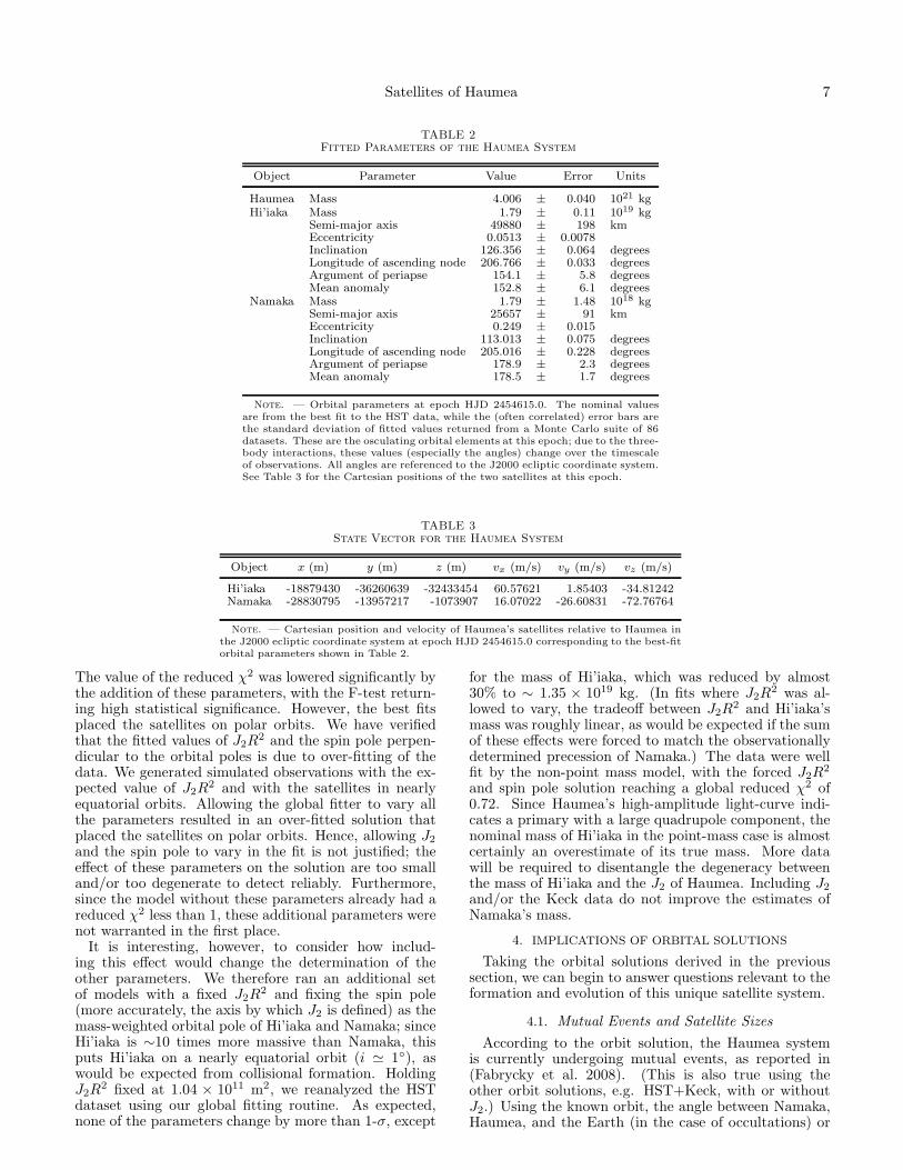
TABLE 2Fitted Parameters of the Haumea System

Object Parameter Value Error Units

Haumea Mass 4.006 ± 0.040 1021 kgHi’iaka Mass 1.79 ± 0.11 1019 kg

Semi-major axis 49880 ± 198 kmEccentricity 0.0513 ± 0.0078Inclination 126.356 ± 0.064 degreesLongitude of ascending node 206.766 ± 0.033 degreesArgument of periapse 154.1 ± 5.8 degreesMean anomaly 152.8 ± 6.1 degrees

Namaka Mass 1.79 ± 1.48 1018 kgSemi-major axis 25657 ± 91 kmEccentricity 0.249 ± 0.015Inclination 113.013 ± 0.075 degreesLongitude of ascending node 205.016 ± 0.228 degreesArgument of periapse 178.9 ± 2.3 degreesMean anomaly 178.5 ± 1.7 degrees

Note. — Orbital parameters at epoch HJD 2454615.0. The nominal valuesare from the best fit to the HST data, while the (often correlated) error bars arethe standard deviation of fitted values returned from a Monte Carlo suite of 86datasets. These are the osculating orbital elements at this epoch; due to the three-body interactions, these values (especially the angles) change over the timescaleof observations. All angles are referenced to the J2000 ecliptic coordinate system.See Table 3 for the Cartesian positions of the two satellites at this epoch.

TABLE 3State Vector for the Haumea System

Object x (m) y (m) z (m) vx (m/s) vy (m/s) vz (m/s)

Hi’iaka -18879430 -36260639 -32433454 60.57621 1.85403 -34.81242Namaka -28830795 -13957217 -1073907 16.07022 -26.60831 -72.76764

Note. — Cartesian position and velocity of Haumea’s satellites relative to Haumea inthe J2000 ecliptic coordinate system at epoch HJD 2454615.0 corresponding to the best-fitorbital parameters shown in Table 2.

The value of the reduced χ2 was lowered significantly bythe addition of these parameters, with the F-test return-ing high statistical significance. However, the best fitsplaced the satellites on polar orbits. We have verifiedthat the fitted values of J2R

2 and the spin pole perpen-dicular to the orbital poles is due to over-fitting of thedata. We generated simulated observations with the ex-pected value of J2R

2 and with the satellites in nearlyequatorial orbits. Allowing the global fitter to vary allthe parameters resulted in an over-fitted solution thatplaced the satellites on polar orbits. Hence, allowing J2

and the spin pole to vary in the fit is not justified; theeffect of these parameters on the solution are too smalland/or too degenerate to detect reliably. Furthermore,since the model without these parameters already had areduced χ2 less than 1, these additional parameters werenot warranted in the first place.

It is interesting, however, to consider how includ-ing this effect would change the determination of theother parameters. We therefore ran an additional setof models with a fixed J2R

2 and fixing the spin pole(more accurately, the axis by which J2 is defined) as themass-weighted orbital pole of Hi’iaka and Namaka; sinceHi’iaka is ∼10 times more massive than Namaka, thisputs Hi’iaka on a nearly equatorial orbit (i ≃ 1), aswould be expected from collisional formation. HoldingJ2R

2 fixed at 1.04 × 1011 m2, we reanalyzed the HSTdataset using our global fitting routine. As expected,none of the parameters change by more than 1-σ, except

for the mass of Hi’iaka, which was reduced by almost30% to ∼ 1.35 × 1019 kg. (In fits where J2R

2 was al-lowed to vary, the tradeoff between J2R

2 and Hi’iaka’smass was roughly linear, as would be expected if the sumof these effects were forced to match the observationallydetermined precession of Namaka.) The data were wellfit by the non-point mass model, with the forced J2R

2

and spin pole solution reaching a global reduced χ2 of0.72. Since Haumea’s high-amplitude light-curve indi-cates a primary with a large quadrupole component, thenominal mass of Hi’iaka in the point-mass case is almostcertainly an overestimate of its true mass. More datawill be required to disentangle the degeneracy betweenthe mass of Hi’iaka and the J2 of Haumea. Including J2

and/or the Keck data do not improve the estimates ofNamaka’s mass.

4. IMPLICATIONS OF ORBITAL SOLUTIONS

Taking the orbital solutions derived in the previoussection, we can begin to answer questions relevant to theformation and evolution of this unique satellite system.

4.1. Mutual Events and Satellite Sizes

According to the orbit solution, the Haumea systemis currently undergoing mutual events, as reported in(Fabrycky et al. 2008). (This is also true using theother orbit solutions, e.g. HST+Keck, with or withoutJ2.) Using the known orbit, the angle between Namaka,Haumea, and the Earth (in the case of occultations) or

8 Ragozzine & Brown

Fig. 3.— Normalized residuals of the three-point mass fit toHST-data only. Plotted is (∆xmod−∆xobs)/σ∆x versus (∆ymod−

∆yobs)/σ∆y for Hi’iaka (diamonds) and Namaka (circles). Pointsthat lie within the circle indicate where the model and observationsvary by less than 1 error bar. See also Figure 2. The residualsare roughly evenly spaced and favor neither Hi’iaka nor Namaka,implying that there are no major systematic effects plaguing thethree-body fit. As reported in the text this solution has a reducedχ2

redof 0.64.

the Sun (in the case of shadowing) falls well below the∼13 milliarcseconds (∼500 km) of the projected shortestaxis of Haumea. Observing multiple mutual events canyield accurate and useful measurements of several systemproperties as shown by the results of the Pluto-Charonmutual event season (e.g. Binzel & Hubbard 1997).The depth of an event where Namaka occults Haumealeads to the ratio of albedos and, potentially, a surfacealbedo map of Haumea, which is known to exhibit colorvariations as a function of rotational phase, indicative ofa variegated surface (Lacerda et al. 2008; Lacerda 2008).Over the course of a single season, Namaka will traverseseveral chords across Haumea allowing for a highlyaccurate measurement of Haumea’s size, shape, and spinpole direction (e.g., Descamps et al. 2008). The precisetiming of mutual events will also serve as extremelyaccurate astrometry, allowing for an orbital solutionmuch more precise than reported here. We believethat incorporating these events into our astrometricmodel will be sufficient to independently determine themasses of all three bodies and J2R

2. Our solution alsopredicts a satellite-satellite mutual event in July 2009 —the last such event until the next mutual event seasonbegins around the year 2100. Our knowledge of thestate of the Haumea system will improve significantlywith the observation and analysis of these events. Seehttp://web.gps.caltech.edu/∼mbrown/2003EL61/mutualfor up-to-date information on the Haumea mutual events.Note that both the mutual events and the three-bodynature of the system are valuable for independentlychecking the astrometric analysis, e.g. by refining platescales and rotations.

Using the best-fit mass ratio and the photometry de-rived in Section 2, we can estimate the range of albedos

Fig. 4.— Relationship between radius, density, and albedo forHi’iaka (left) and Namaka (right). A range of possible albedosand densities can reproduce the determined mass and brightnessratios of Hi’iaka and Namaka, which are assumed to be spheri-cal. The solid lines show the relationship for the nominal masses,reported in Table 2, with dotted lines showing the 1-σ mass er-ror bars. Note that the mass of both Hi’iaka and Namaka maybe overestimated (due to insufficient data, see Section 3). Thealbedo and density of the Rabinowitz et al. (2006) edge-on modelfor Haumea are shown by dotted lines. Both satellites must havelower densities and/or higher albedos than Haumea. The similarspectral (Barkume et al. 2006) and photometric (Fraser & Brown2009) properties of Haumea, Hi’iaka, and Namaka indicate thattheir albedos should be similar. Under the assumption that thesatellites have similar albedos to Haumea, the densities of thesatellites indicate that they are primarily composed of water ice(ρ ≈ 1.0 g/cc). Low satellite densities would bolster the hypothe-sis that the satellites formed from the collisional remnants of thewater ice mantle of the differentiated proto-Haumea. Observationof Haumea-Namaka mutual events will allow for much more preciseand model-independent measurements of Namaka’s radius, density,and albedo.

and densities for the two satellites. The results of thiscalculation are shown in Figure 4. The mass and bright-ness ratios clearly show that the satellites must eitherhave higher albedos or lower densities than Haumea; thedifference is probably even more significant than shownin Figure 4 since the nominal masses of Hi’iaka and Na-maka are probably overestimated (see Section 3). Thesimilar spectral (Barkume et al. 2006) and photometric(Fraser & Brown 2009) properties of Haumea, Hi’iaka,and Namaka indicate that their albedos should be sim-ilar. Similar surfaces are also expected from rough cal-culations of ejecta exchange discussed by Stern (2009),though Benecchi et al. (2008) provide a contrary view-point. If the albedos are comparable, the satellite den-sities indicate a mostly water ice composition (ρ ≈ 1.0g/cc). This lends support to the hypothesis that thesatellites are formed from a collisional debris disk com-posed primarily of water ice from the shattered mantleof Haumea. This can be confirmed in the future with adirect measurement of Namaka’s size from mutual eventphotometry. Assuming a density of water ice, the es-timated radii of Hi’iaka and Namaka are ∼160 km and∼80 km, respectively.

4.2. Long-term Orbital Integrations

It is surprising to find the orbits in an excited state,both with non-zero eccentricities and with a rather largemutual inclination. In contrast the regular satellite sys-

Satellites of Haumea 9

tems of the gas giants, the satellites of Mars, the threesatellites of Pluto (Tholen et al. 2008), and asteroid triplesystems with well known orbits (Marchis et al. 2005) areall in nearly circular and co-planar orbits. In systemsof more than one satellite, perturbations between thesatellites produce forced eccentricities and inclinationsthat will remain even with significant damping. If theexcited state of the Haumea system is just a reflectionof normal interactions, then there will be small free ec-centricities and inclinations, which can be estimated byintegrating the system for much longer than the preces-sion timescales and computing the time average of theseelements. Using this technique, and exploring the entireMonte Carlo suite of orbital solutions, we find that thefree eccentricity of Hi’iaka is ∼0.07, the free eccentric-ity of Namaka is ∼ 0.21, and the time-averaged mutualinclination is ∼12.5. Non-zero free eccentricities and in-clinations imply that the excited state of the system isnot due to satellite-satellite perturbations. These inte-grations were calculated using the n-body code SyMBA(Levison & Duncan 1994) using the regularized mixedvariable symplectic method based on the mapping byWisdom & Holman (1991). Integration of all the MonteCarlo orbits showed for ∼2000-years showed no signs ofinstability, though we do note that the system chaoticallyenters and exits the 8:3 resonance. The orbital solutionsincluding J2R

2 ≃ 1.04 × 1011 m2 were generally morechaotic, but were otherwise similar to the point-mass in-tegrations.

These integrations did not include the effect of theSun, which adds an additional minor torque to the sys-tem that is negligible (∆Ω ∼ 10−5 degrees) over thetimescale of observations. The effects of the sun on thesatellite orbits on long-time scales were not investigated.While the relative inclination between the satellite or-bits and Haumea’s heliocentric orbit (∼119 for Hi’iakaand ∼105 for Namaka) places this system in the regimewhere the Kozai effect can be important (Kozai 1962;Perets & Naoz 2008), the interactions between the satel-lites are strong enough to suppress weak Kozai oscilla-tions due to the Sun, which are only active in the absenceof other perturbations (Fabrycky & Tremaine 2007).

We did not include any correction to our solution forpossible differences between the center of light (more pre-cisely, the center of fitted PSF) and center of mass ofHaumea. This may be important since Lacerda et al.(2008) find that Haumea’s two-peaked light curve can beexplained by a dark red albedo feature, which could po-tentially introduce an systematic astrometric error. TheFebruary 2007 Hubble data and March 2008 Keck data,both of which span a full rotation, do not require acenter-of-light/center-of-mass correction for a good fit,implying that the correction should be smaller than ∼2milliarcseconds (i.e. ∼70 km). Examination of the all theastrometric residuals and a low reduced-χ2 confirm thatcenter-of-light/center-of-mass corrections are not signif-icant at our level of accuracy. For Pluto and Charon,albedo features can result in spurious orbital astrometrybecause Pluto and Charon are spin-locked; this is not thecase for Haumea. For Keck observations where Namakais not detected (see Table 1), it is usually because of lowsignal-to-noise and Namaka’s calculated position is notnear Haumea. In the cases where Namaka’s light con-taminates Haumea, the induced photocenter error would

be less than the observed astrometric error.

4.3. Tidal Evolution

All of the available evidence points to a scenario for theformation of Haumea’s satellites similar to the formationof the Earth’s moon: a large oblique collision created adisk of debris composed mostly of the water ice man-tle of a presumably differentiated proto-Haumea. Tworelatively massive moons coalesced from the predomi-nantly water-ice disk near the Roche lobe. Interestingly,in studying the formation of Earth’s Moon, about onethird of the simulations of Ida et al. (1997) predict theformation of two moonlets with the outer moonlet ∼10times more massive the inner moonlet. Although thedisk accretion model used by Ida et al. (1997) made theuntenable assumption that the remnant disk would im-mediately coagulate into solid particles, the general ideathat large disks with sufficient angular momentum couldresult in two separate moons seems reasonable. Suchcollisional satellites coagulate near the Roche lobe (e.g.a distances of ∼3-5 primary radii) in nearly circular or-bits and co-planar with the (new) rotational axis of theprimary. For Haumea, the formation of the satellites ispresumably concurrent with the formation of the fam-ily billions of years ago (Ragozzine & Brown 2007) andthe satellites have undergone significant tidal evolutionto reach their current orbits (B05).

4.3.1. Tidal Evolution of Semi-major Axes

The equation for the typical semi-major axis tidal ex-pansion of a single-satellite due to primary tides is (Mur-ray & Dermott 2000):

a =3k2p

Qpq

(

Rp

a

)5

na (2)

where k2p is the second-degree Love number of the pri-mary, Qp is the primary tidal dissipation parameter (see,e.g., Goldreich & Soter 1966), q is the mass ratio, Rp isthe primary radius, a is the satellite semi-major axis, and

n ≡

√

GMtot

a3 is the satellite mean motion. As pointed out

by B05, applying this equation to Hi’iaka’s orbit (usingthe new-found q = 0.0045) indicates that Haumea mustbe extremely dissipative: Qp ≃ 17, averaged over the ageof the solar system, more dissipative than any known ob-ject except ocean tides on the present-day Earth. Thishigh dissipation assumes an unrealistically high k2 ≃ 1.5,which would be achieved only if Haumea were perfectlyfluid. Using the strength of an rocky body and the Yo-der (1995) method of estimating k2, Haumea’s estimatedk2p is ∼ 0.003. Such a value of k2p would imply a ab-surdly low and physically implausible Qp ≪ 1. StartingHi’iaka on more distant orbits, e.g. the current orbit ofNamaka, does not help much in this regard since the tidalexpansion at large semi-major axes is the slowest part ofthe tidal evolution. There are three considerations, how-ever, that may mitigate the apparent requirement of anastonishingly dissipative Haumea. First, if tidal forcingcreates a tidal bulge that lags by a constant time (asin Mignard 1980), then Haumea’s rapid rotation (whichhardly changes throughout tidal evolution) would natu-rally lead to a significant increase in tidal evolution. Inother words, if Qp is frequency dependent (as it seems to

10 Ragozzine & Brown

be for solid bodies, see Efroimsky & Lainey 2007)), thenan effective Q of ∼16 may be equivalent to an objectwith a one-day rotation period maintaining an effectiveQ of 100, the typically assumed value for icy solid bodies.That is, Haumea’s higher-than-expected dissipation maybe related to its fast rotation. Second, the above calcu-lation used the volumetric radius Rp ≃ 650 km, in cal-culating the magnitude of the tidal bulge torque, wherewe note that Equation 2 assumes a spherical primary. Acomplete calculation of the actual torque caused by tidalbulges on a highly non-spherical body is beyond the scopeof this paper, but it seems reasonable that since tidalbulges are highly distance-dependent, the volumetric ra-dius may lead to an underestimate in the tidal torque andresulting orbital expansion. Using Rp ≃ 1000 km, likelyan overestimate, allows k2p/Qp to go down to 7.5×10−6,consistent both with k2p ≃ 0.003 and Qp ≃ 400. Clearly,a reevaluation of tidal torques and the resulting orbitalchange for satellites around non-spherical primaries iswarranted before making assumptions about the tidalproperties of Haumea.

The third issue that affects Hi’iaka’s tidal evolutionis Namaka. While generally the tidal evolution of thetwo satellites is independent, if the satellites form a res-onance it might be possible to boost the orbital expan-sion of Hi’iaka via angular momentum transfer with themore tidally affected Namaka. (Note that applying thesemi-major axis evolution questions to Namaka requiresa somewhat less dissipative primary, i.e. Qp values ∼8times larger than discussed above.) Even outside of reso-nance, forced eccentricities can lead to higher dissipationin both satellites, somewhat increasing the orbital expan-sion rate. Ignoring satellite interactions and applyingEquation 2 to each satellite results in the expected rela-tionship between the mass ratio and the semi-major axisratio of (Canup et al. 1999; Murray & Dermott 2000):

m1

m2≃

(

a1

a2

)13/2

(3)

where evaluating the right-hand side using the deter-mined orbits implies that m1

m2≃ 75.4±0.4. This mass ra-

tio is highly inconsistent with a brightness ratio of ∼3.7for the satellites, implying that the satellites have notreached the asymptotic tidal end-state. Equation 3 isalso diagnostic of whether the tidally-evolving satellitesare on converging or diverging orbits: that the left-handside of Equation 3 is greater than the right-hand side im-plies that the satellites are on convergent orbits, i.e. theratio of semi-major axes is increasing and the ratio of theorbital periods is decreasing (when not in resonance).

4.3.2. Tidal Evolution of Eccentricities and Inclinations

Turning now from the semi-major axis evolution, weconsider the unexpectedly large eccentricities and non-zero inclination of the Namaka and Hi’iaka. None of theaforementioned considerations can explain the highly ex-cited state of the Haumea satellite system. As pointedout by B05, a simple tidal evolution model would requirethat the eccentricities and, to some extent, inclinationsare significantly damped when the satellites are closer toHaumea, as eccentricity damping is more efficient thansemi-major axis growth. One would also expect that thesatellites formed from a collision disk with low relative

inclinations. So, while a mutual inclination of 13 is un-likely to occur by random capture, a successful model forthe origin of the satellites must explain why the satellitesare relatively far from co-planar.

The unique current orbital state of the Haumea sys-tem is almost certainly due to a unique brand of tidalevolution. Terrestrial bodies are highly dissipative, butnone (except perhaps some asteroid or KBO triple sys-tems) have large significantly interacting satellites. Onthe other hand, gas giant satellite systems have multi-ple large interacting satellites, but very low dissipationand hence slow semi-major axis change. The change insemi-major axes is important because it causes a largechange in the period ratio, allowing the system to crossmany resonances, which can strongly change the natureof the system and its evolution. Even though Haumea isin a distinct niche of tidal parameter space, we can gaininsights from studies of other systems, such as the evolu-tion of satellites in the Uranian system (e.g., Tittemore& Wisdom 1988, 1989; Dermott et al. 1988; Malhotra &Dermott 1990) or the interactions of tidally-evolving ex-oplanets (e.g., Wu & Goldreich 2002; Ferraz-Mello et al.2003). In addition, since the results of some Moon-forming impacts resulted in the creation of two moons(Ida et al. 1997), Canup et al. (1999) studied the tidalevolution of an Earth-Moon-moon system, in many wayssimilar to the Haumea system.

Using the results of these former investigations, we canqualitatively explain the excited state of the Haumeansystem. As the satellites were evolving outward at dif-ferent rates, the ratio of orbital periods would periodi-cally reach a resonant ratio. For example, as the currentsystem is in/near the 8:3 resonance, it probably passedthrough the powerful 3:1 resonance in the relatively re-cent past. Since the satellites are on convergent orbits,they would generally get caught into these past reso-nances, even if their early eccentricities and inclinationswere low. Note that this simple picture of resonance cap-ture must be investigated numerically (as in, e.g., Titte-more & Wisdom 1988) and that higher-order resonancesmay act differently from lower-order resonances (Zhang& Hamilton 2008). Further semi-major axis growth whiletrapped in the resonance rapidly pumps eccentricitiesand/or inclinations, depending on the type of resonance(e.g., Ward & Canup 2006). This continues until thesatellites chaotically escape from the resonance. Escap-ing could be a result of either excitation (related to sec-ondary resonances, see Tittemore & Wisdom 1989; Mal-hotra & Dermott 1990) and/or chaotic instability dueto overlapping sub-resonances, split by the large J2 ofHaumea (Dermott et al. 1988). Outside of resonances,tidal dissipation in the satellites can damp eccentrici-ties while the satellites are close to Haumea, but at theircurrent positions, eccentricity damping is very ineffectiveeven for highly dissipative satellites. Inclination damp-ing is generally slower than eccentricity damping and wasprobably small even when the satellites were much closerto Haumea. Therefore a “recent” excitation by passagethrough a resonance (possibly the 3:1) can qualitativelyexplain the current orbital configuration, which has nothad the time to tidally damp to a more circular co-planarstate. Numerical integrations will be needed to trulyprobe the history of this intriguing system and may beable to constrain tidal parameters of Haumea, Hi’iaka,

Satellites of Haumea 11

and/or Namaka.Note that early in the history of this system when the

satellites were orbiting at much smaller semi-major axes(a . 10Rp), the tri-axial nature of the primary wouldhave been much more important and could have sig-nificantly affected the satellite orbits (Scheeres 1994).At some point during semi-major axis expansion secularresonances (such as the evection resonance) could alsobe important for exciting eccentricities and/or inclina-tions (Touma & Wisdom 1998). Finally, tides raised onHaumea work against eccentricity damping; for certaincombinations of primary and satellite values of k2/Q,tides on Haumea can pump eccentricity faster than it isdamped by the satellites (especially if Haumea is partic-ularly dissipative). While eccentricity-pumping tides onHaumea may help in explaining the high eccentricities,producing the large mutual inclination (which is hardlyaffected by any tidal torques) is more likely to occur in aresonance passage, as with Miranda in the Uranian sys-tem (Tittemore & Wisdom 1989; Dermott et al. 1988).

5. CONCLUSIONS

Using new observations from the Hubble Space Tele-scope, we have solved for the orbits and masses of thetwo dynamically interacting satellites of the dwarf planetHaumea. A three-body model, using the parameters witherrors given in Table 2, provides an excellent match to theprecise relative astrometry given in Table 1. The orbitalparameters of Hi’iaka, the outer, brighter satellite matchwell the orbit previously derived in Brown et al. (2005).The newly derived orbit of Namaka, the inner, faintersatellite has a surprisingly large eccentricity (0.249 ±

0.015) and mutual inclination to Hi’iaka of (13.41 ±

0.08). The eccentricities and inclinations are not due tomutual perturbations, but can be qualitatively explainedby tidal evolution of the satellites through mean-motionresonances. The precession effect of the non-sphericalnature of the elongated primary, characterized by J2,cannot be distinguished from the precession caused bythe outer satellite in the current data.

The orbital structure of Haumea’s satellites is unlikelyto be produced in a capture-related formation mechanism(e.g., Goldreich et al. 2002). Only the collisional forma-tion hypothesis (allowing for reasonable, but atypical,tidal evolution) can explain the nearly co-planar satel-lites (probably with low densities), the rapid spin andelongated shape of Haumea (Rabinowitz et al. 2006), and

the Haumea collisional family of icy objects with similarsurfaces and orbits (Brown et al. 2007).

The future holds great promise for learning more aboutthe Haumea system, as the orbital solution indicates thatNamaka and Haumea are undergoing mutual events forthe next several years. This will provide excellent obser-vational constraints on the size, shape, spin pole, density,and internal structure of Haumea and direct measure-ments of satellite radii, densities, and albedos. Thereare also interesting avenues for future theoretical inves-tigations, especially into the unique nature of tidal evo-lution in the Haumean system. These insights into theformation and evolution of the Haumean system can becombined with our understanding of other Kuiper beltbinaries to investigate how these binaries form and tofurther decipher the history of the outer solar system.

We would like to thank Meg Schwamb, Aaron Wolf,Matt Holman, and others for valuable discussions andEugene Fahnestock for kindly providing his code for grav-ity around tri-axial bodies. We also acknowledge obser-vational support from Emily Schaller and Chad Trujillo.We especially acknowledge the encouragement and dis-cussions of Dan Fabrycky. DR is grateful for the supportof the Moore Foundation. This work was also supportedby NASA Headquarters under the Earth and SpaceSciences Fellowship and the Planetary Astronomy pro-grams. This work is based on NASA/ESA Hubble SpaceTelescope program 11518 using additional data from pro-grams 10545, 10860, and 11169. Support for all theseprograms was provided by NASA through grants HST-GO-10545, HST-GO-10860, HST-G0-11518, and HST-GO-11169 from the Space Telescope Science Institute(STScI), which is operated by the Association of Univer-sities for Research in Astronomy, Inc., under NASA con-tract NAS 5-26555. Some data presented herein was ob-tained at the W. M. Keck Observatory, which is operatedas a scientific partnership among the California Instituteof Technology, the University of California, and the Na-tional Aeronautics and Space Administration. The ob-servatory was made possible by the generous financialsupport of the W. M. Keck Foundation. The authorswish to recognize and acknowledge the very significantcultural role and reverence that the summit of MaunaKea has always had within the indigenous Hawaiian com-munity. We are most fortunate to have the opportu-nity to conduct observations of Haumea, Hi’iaka, andNamaka, which were named after Hawaiian goddesses.

REFERENCES

Anderson, J., & King, I. R. 2003, PASP, 115, 113Astakhov, S. A., Lee, E. A., & Farrelly, D. 2005, MNRAS, 360,

401. astro-ph/0504060Barkume, K. M., Brown, M. E., & Schaller, E. L. 2006, ApJ, 640,

L87. arXiv:astro-ph/0601534Benecchi, S. D., Noll, K. S., Grundy, W. M., Buie, M. W., Stephens,

D. C., & Levison, H. F. 2008, ArXiv e-prints. 0811.2104Binzel, R. P., & Hubbard, W. B. 1997, Pluto and Charon, ed. S.A.

Stern, D.J Tholen (U. Arizona Press:1997)Brown, M. E. 2008, The Largest Kuiper Belt Objects (The Solar

System Beyond Neptune), 335Brown, M. E., Barkume, K. M., Ragozzine, D., & Schaller, E. L.

2007, Nature, 446, 294Brown, M. E., Bouchez, A. H., Rabinowitz, D., Sari, R., Trujillo,

C. A., van Dam, M., Campbell, R., Chin, J., Hartman, S.,Johansson, E., Lafon, R., Le Mignant, D., Stomski, P., Summers,D., & Wizinowich, P. 2005, ApJ, 632, L45

Brown, M. E., & Schaller, E. L. 2007, Science, 316, 1585

Brown, M. E., & Suer, T.-A. 2007, IAU Circ., 8812, 1Brown, M. E., & Trujillo, C. A. 2004, AJ, 127, 2413Brown, M. E., van Dam, M. A., Bouchez, A. H., Le Mignant, D.,

Campbell, R. D., Chin, J. C. Y., Conrad, A., Hartman, S. K.,Johansson, E. M., Lafon, R. E., Rabinowitz, D. L., Stomski, P. J.,Jr., Summers, D. M., Trujillo, C. A., & Wizinowich, P. L. 2006,ApJ, 639, L43. arXiv:astro-ph/0510029

Canup, R. M. 2005, Science, 307, 546Canup, R. M., Levison, H. F., & Stewart, G. R. 1999, AJ, 117, 603Dermott, S. F., Malhotra, R., & Murray, C. D. 1988, Icarus, 76,

295Descamps, P., Marchis, F., Pollock, J., Berthier, J., Vachier, F.,

Birlan, M., Kaasalainen, M., Harris, A. W., Wong, M. H.,Romanishin, W. J., Cooper, E. M., Kettner, K. A., Wiggins,P., Kryszczynska, A., Polinska, M., Coliac, J.-F., Devyatkin,A., Verestchagina, I., & Gorshanov, D. 2008, Icarus, 196, 578.0710.1471

12 Ragozzine & Brown

Efroimsky, M., & Lainey, V. 2007, Journal of Geophysical Research(Planets), 112, 12003. 0709.1995

Fabrycky, D., & Tremaine, S. 2007, ApJ, 669, 1298. 0705.4285Fabrycky, D. C., Ragozzine, D., Brown, M. E., & Holman, M. J.

2008, IAU Circ., 8949, 1Ferraz-Mello, S., Beauge, C., & Michtchenko, T. A. 2003, Celestial

Mechanics and Dynamical Astronomy, 87, 99. arXiv:astro-ph/0301252

Fraser, W. C., & Brown, M. E. submitted, 2009Funato, Y., Makino, J., Hut, P., Kokubo, E., & Kinoshita, D. 2004,

Nature, 427, 518. arXiv:astro-ph/0402328Ghez, A. M., Salim, S., Weinberg, N. N., Lu, J. R., Do, T., Dunn,

J. K., Matthews, K., Morris, M. R., Yelda, S., Becklin, E. E.,Kremenek, T., Milosavljevic, M., & Naiman, J. 2008, ApJ, 689,1044. 0808.2870

Goldreich, P., Lithwick, Y., & Sari, R. 2002, Nature, 420, 643.arXiv:astro-ph/0208490

Goldreich, P., & Soter, S. 1966, Icarus, 5, 375Greenberg, R., & Barnes, R. 2008, Icarus, 194, 847Grundy, W. M., Noll, K. S., Buie, M. W., Benecchi, S. D., Stephens,

D. C., & Levison, H. F. 2008, ArXiv e-prints. 0812.3126He lminiak, K., & Konacki, M. 2008, ArXiv e-prints. 0807.4139Holsapple, K. A. 2007, Icarus, 187, 500Ida, S., Canup, R. M., & Stewart, G. R. 1997, Nature, 389, 353Kozai, Y. 1962, AJ, 67, 591Lacerda, P. 2008, ArXiv e-prints. 0811.3732Lacerda, P., Jewitt, D., & Peixinho, N. 2008, AJ, 135, 1749.

0801.4124Lacerda, P., & Jewitt, D. C. 2007, AJ, 133, 1393. arXiv:astro-

ph/0612237Levison, H. F., & Duncan, M. J. 1994, Icarus, 108, 18Levison, H. F., Morbidelli, A., Vokrouhlicky, D., & Bottke, W. F.

2008, AJ, 136, 1079. 0809.0553Levison, H. F., & Stern, S. A. 2001, AJ, 121, 1730. astro-

ph/0011325Malhotra, R., & Dermott, S. F. 1990, Icarus, 85, 444Marchis, F., Descamps, P., Hestroffer, D., & Berthier, J. 2005,

Nature, 436, 822Mignard, F. 1980, Moon and the Planets, 23, 185Murray, C. D., & Dermott, S. F. 2000, Solar System Dynamics

(Cambridge University Press)Nesvorny, D. 2008, in AAS/Division for Planetary Sciences

Meeting Abstracts, vol. 40 of AAS/Division for PlanetarySciences Meeting Abstracts, 38.02

Nesvorny, D., & Roig, F. 2001, Icarus, 150, 104Noll, K. S., Grundy, W. M., Stephens, D. C., Levison, H. F., &

Kern, S. D. 2008, Icarus, 194, 758. 0711.1545Perets, H. B., & Naoz, S. 2008, ArXiv e-prints. 0809.2095Press, W. H., Teukolsky, S. A., Vetterling, W. T., & Flannery,

B. P. 1992, Numerical recipes in FORTRAN. The art of scientificcomputing (Cambridge: University Press, —c1992, 2nd ed.)

Rabinowitz, D. L., Barkume, K., Brown, M. E., Roe, H., Schwartz,M., Tourtellotte, S., & Trujillo, C. 2006, ApJ, 639, 1238.arXiv:astro-ph/0509401

Rabinowitz, D. L., Schaefer, B. E., Schaefer, M., & Tourtellotte,S. W. 2008, AJ, 136, 1502. 0804.2864

Ragozzine, D., & Brown, M. E. 2007, AJ, 134, 2160. 0709.0328Schaller, E. L., & Brown, M. E. 2008, ApJ, 684, L107. 0808.0185Scheeres, D. J. 1994, Icarus, 110, 225Stansberry, J., Grundy, W., Brown, M., Cruikshank, D., Spencer,

J., Trilling, D., & Margot, J.-L. 2008, Physical Properties ofKuiper Belt and Centaur Objects: Constraints from the SpitzerSpace Telescope (The Solar System Beyond Neptune), 161

Stephens, D. C., & Noll, K. S. 2006, AJ, 131, 1142. arXiv:astro-ph/0510130

Stern, S. A. 2009, Icarus, 199, 571. 0805.3482Stern, S. A., Weaver, H. A., Steffl, A. J., Mutchler, M. J., Merline,

W. J., Buie, M. W., Young, E. F., Young, L. A., & Spencer, J. R.2006, Nature, 439, 946

Tholen, D. J., Buie, M. W., Grundy, W. M., & Elliott, G. T. 2008,AJ, 135, 777. 0712.1261

Tittemore, W. C., & Wisdom, J. 1988, Icarus, 74, 172— 1989, Icarus, 78, 63Touma, J., & Wisdom, J. 1998, AJ, 115, 1653Ward, W. R., & Canup, R. M. 2006, Science, 313, 1107Weaver, H. A., Stern, S. A., Mutchler, M. J., Steffl, A. J., Buie,

M. W., Merline, W. J., Spencer, J. R., Young, E. F., & Young,L. A. 2006, Nature, 439, 943. astro-ph/0601018

Weidenschilling, S. J. 2002, Icarus, 160, 212Wisdom, J., & Holman, M. 1991, AJ, 102, 1528Wu, Y., & Goldreich, P. 2002, ApJ, 564, 1024. arXiv:astro-

ph/0108499Yoder, C. F. 1995, 1Zhang, K., & Hamilton, D. P. 2008, Icarus, 193, 267