Embed Size (px)
Citation preview
D. R. WiltonECE Dept.
ECE 6382 ECE 6382
Green’s Functions in Two and Three Dimensions
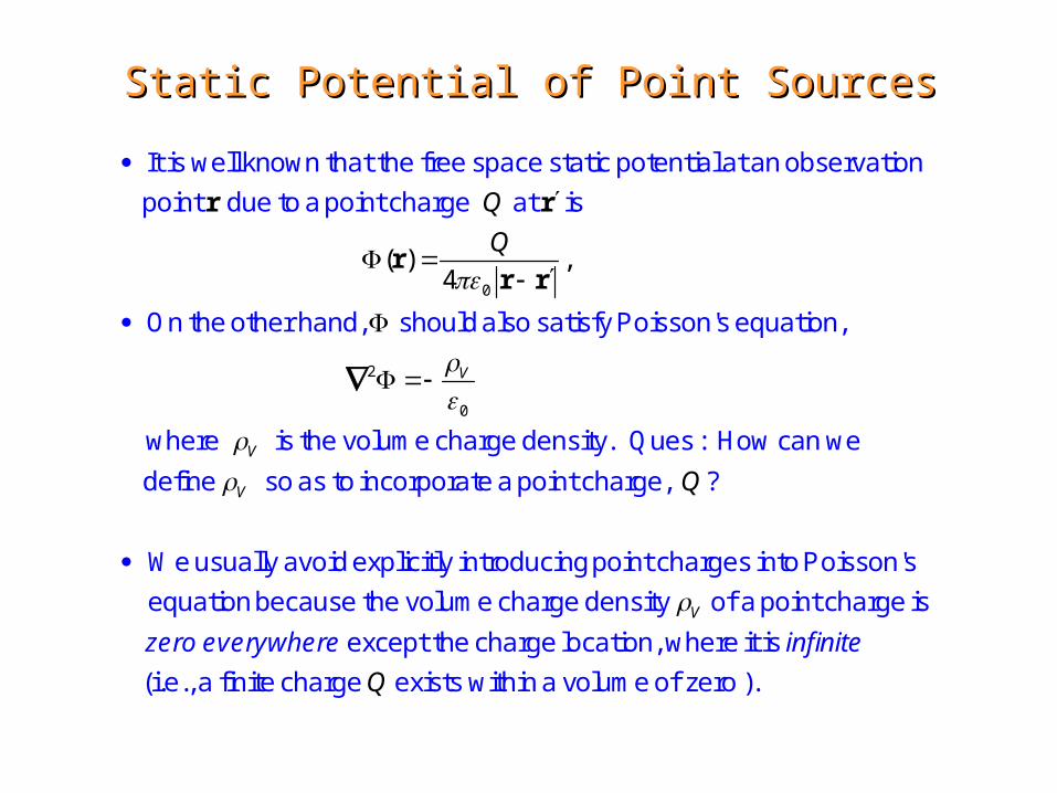
Static Potential of Point SourcesStatic Potential of Point Sources
0
2
0
( ) ,4
V
Q
Q
r r
rr r
It is well known that the free space static potential at an observation
point due to a point charge at is
On the other hand, should also satisfy Poisson's equation,
V
V Q
where is the volume charge density. Ques : How can we
define so as to incorporate a point charge, ?
We usually avoid explicitly introducing point charges into Poisson's
equation be
caus V
Q
e the volume charge density of a point charge is
except the charge location, where it is
(i.e., a finite charge exists within a volume of zero ).
zero everywhere infinite
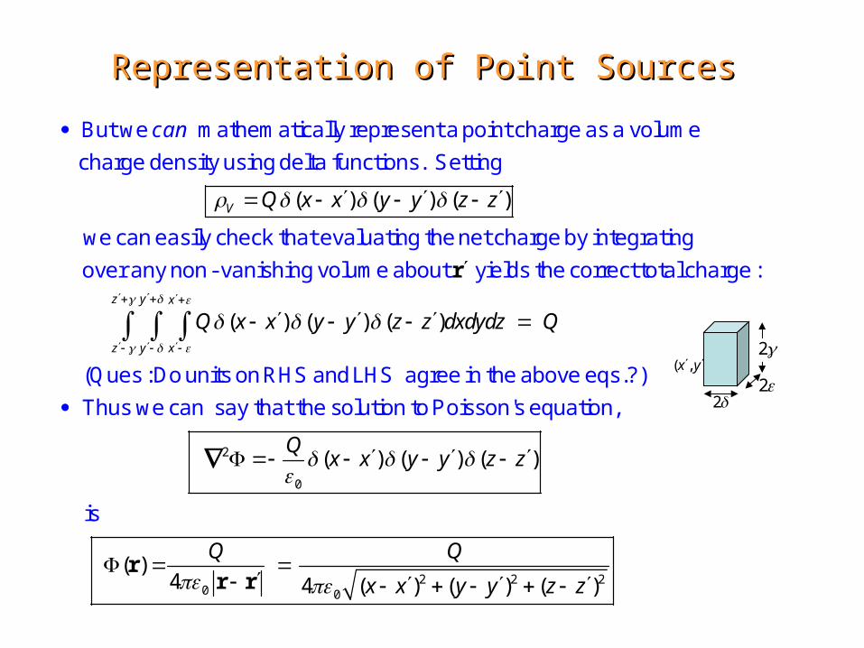
Representation of Point Sources Representation of Point Sources
( ) ( ) ( )V Q x x y y z z
But we mathematically represent a point charge as a volume
charge density using delta functions. Setting
we can easily check that evaluating the net charge by integrating
can
( ) ( ) )
( )
(yz x
z y x
Q x x y y z z dxdydz Q
r
over any non- vanishing volume about yields the correct total charge :
Ques : Do units on RHS and LHS agree in the above eqs.?
Thus we can
2
0
2 2 20 0
( ) ( ) ( )
( )4 4 ( ) ( ) ( )
Qx x y y z z
Q Q
x x y y z z
rr r
say that the solution to Poisson's equation,
is
22
2( , , )x y z
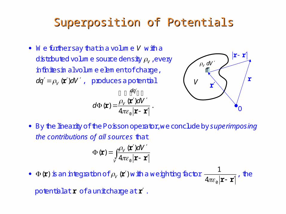
Superposition of PotentialsSuperposition of Potentials
0
( )
( )( ) .
4
V
V
V
dq
V
dq dV
dVd
r
rr
r r
We further say that in a volume with a
distributed volume source density , every
infinitesimal volume element of charge,
, produces a potential
By th
0
0
( )( )
4
1( ) ( )
4
V
V
V
dV
r
rr r
r rr r
e linearity of the Poisson operator, we conclude by
that
is an integration of with a weighting factor , t
superimposing
the contributions of all sources
r r
he
potential at of a unit charge at .
rr
r r
V dV
V
O
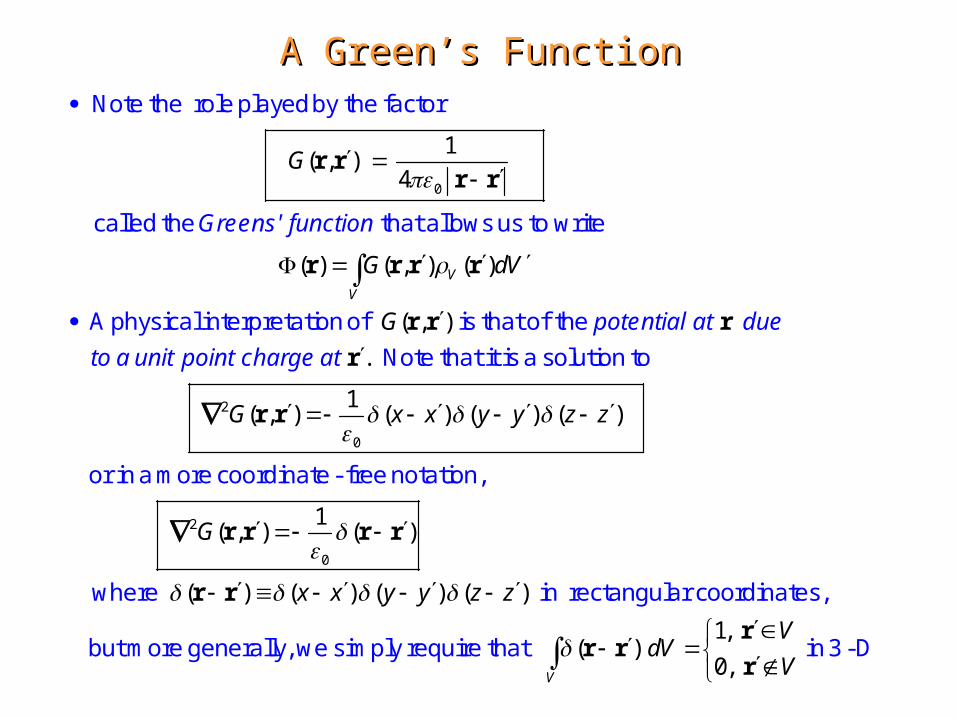
A Green’s FunctionA Green’s Function
0
1( , )
4
( ) ( , ) ( )
( , )
V
V
G
G dV
G
r rr r
r r r r
r r r
Note the role played by the factor
called the that allows us to write
A physical interpretation of is that of the
Greens' function
potential at du
2
0
2
0
.
1( , ) ( ) ( ) ( )
1( , ) ( )
( ) ( ) ( ) ( )
G x x y y z z
G
x x y y z z
r
r r
r r r r
r r
Note that it is a solution to
or in a more coordinate - free notation,
where in rect
e
to a unit point charge at
1,( )
0,V
VdV
V
rr r
r
angular coordinates,
but more generally, we simply require that in 3 -D

Green’s Function ConditionsGreen’s Function Conditions
0 0
2
1 1( , )
4 4
( , ) 0
(
Gr
G r
G
r
r 0r
r 0
To check our claims, it suffices to place at the coordinate origin so
spherical coordinates can be used :
Check that satisfies the homogeneous equation when :
2
22 2
0
1 1 1, )
4
G rr
r r r r r
r 02r
20
2
0 0
2
0 0 0
2
0
1 00, 0
4
1 1( , ) ( ) ,
ˆlim ( , ) lim ( , ) lim ( , )
( , )ˆ ˆlim sin
V V
rV V V
r
rr
G dV dV V
G dV G dV G dS
Gd d
r
r 0 r r 0
r 0 r 0 r 0 n
r 0r r
divergencetheorem
Next, check that encloses :
2
00 0
4lim
4 2
0 2
0
1,
.V
r 0 if encloses
r̂V
V
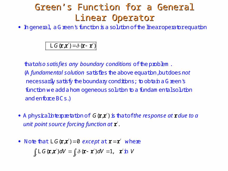
Green’s Function for a General Linear OperatorGreen’s Function for a General Linear Operator
( , ) ( )G
r r r r
In general, a Green's function is a solution of the linear operator equation
that of the problem.
(A satisfies the above e
L
also satisfies any boundary conditions
fundamental solution
quation, but does
necessarily satisfy the boundary conditions; to obtain a Green's
function we add a homogeneous solution to a fundamental solution
and enforce BCs.)
A physical interpreta
not
( , )
.
( , ) 0
( , ) ( ) 1,V V
G
G
G dV dV V
r r r
r
r r r r
r r r r r
tion of is that of
Note that at where
in
L
L
the response at due to a
unit point source forcing function at
except

A Source-Weighted Superposition over the Unit A Source-Weighted Superposition over the Unit Source Response Provides a General Solution Source Response Provides a General Solution
( ) ( ) , ( )
( ) ( , ) ( )V
u f f
u G f dV
r r r
r r r r
The solution to the general problem
a general forcing function,
is then found by a source - weighted superposition of the f 'n response :
To check that this is
-
a so
Lu
u
( ) ( , ) ( ) ( , ) ( )
( ) ( )
( )
V V
V
u G f dV G f dV
f dV
f
r r r r r r r
r r r
r
lution, note that
Lu L L
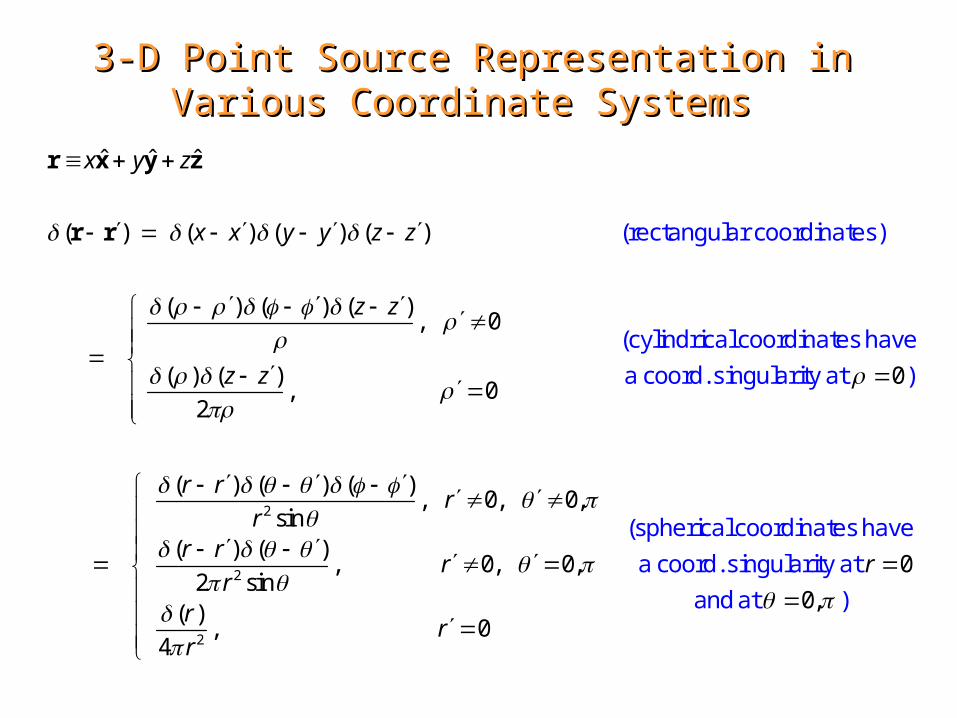
3-D Point Source Representation in Various 3-D Point Source Representation in Various Coordinate Systems Coordinate Systems
ˆ ˆ ˆ
( ) ( ) ( ) ( )
( ) ( ) ( ), 0
( ) ( ) 0, 0
2
( ) ( ) (
x y z
x x y y z z
z z
z z
r r
r x y z
r r (rectangular coordinates)
(cylindrical coordinates have
a coord. singularity at )
2
2
2
), 0, 0,
sin( ) ( )
, 0, 0, 02 sin
0,( ), 0
4
rr
r rr r
rr
rr
(spherical coordinates have
a coord. singularity at
and at )
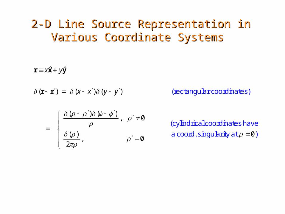
2-D Line Source Representation in Various 2-D Line Source Representation in Various Coordinate Systems Coordinate Systems
ˆ ˆ
( ) ( ) ( )
( ) ( ), 0
( ) 0, 0
2
x y
x x y y
r x y
r r (rectangular coordinates)
(cylindrical coordinates have
a coord. singularity at )
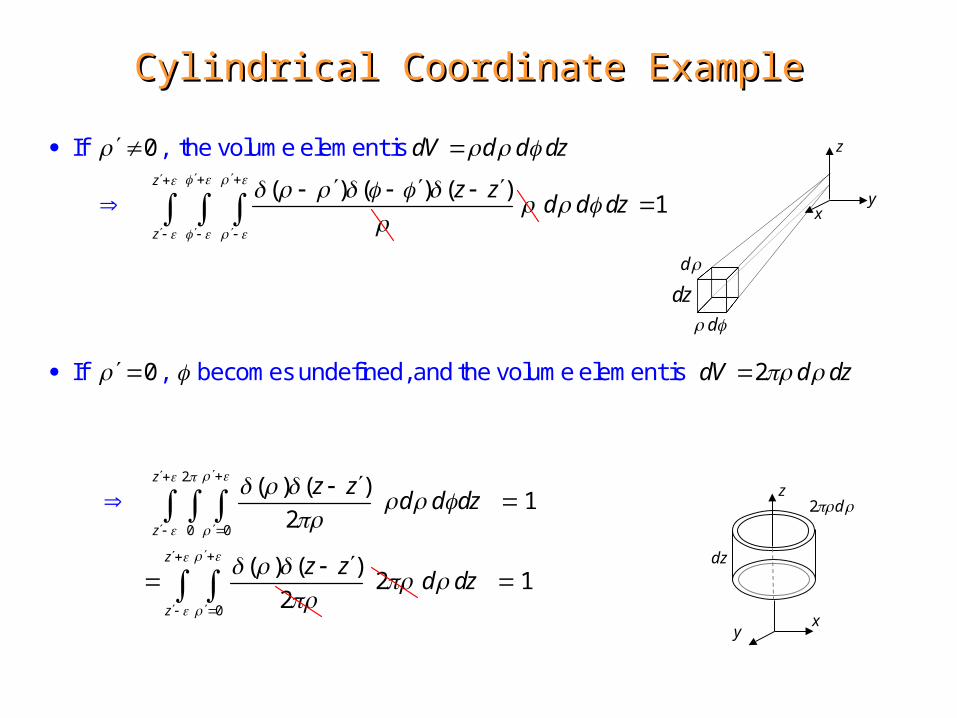
Cylindrical Coordinate ExampleCylindrical Coordinate Example
0
( ) ( ) ( )
dV d d dz
z z
If , the volume element is
2
0 0
1
0 2
( ) ( )1
2
( ) ( )
2
z
z
z
z
d d dz
dV d dz
z zd d dz
z z
If , becomes undefined, and the volume element is
20
1z
z
d dz
d
d dz
xy
z
dz
2 d z
xy
Example: A Simple Static Green’s Function with Example: A Simple Static Green’s Function with Boundary Conditions --- Charge over a Ground Boundary Conditions --- Charge over a Ground
PlanePlane
0 0
( , )
1 1( , )
4 4fundamental solution homogeneous soluti
The potential at due to a unit charge at
can be found from image theory. It is given by
G
G
r r r r
r rr r r r
above a ground plane
2 2
0 0 0
ˆ2 .
0 ( , )
1 1 1( , ) ( , ) ( , ) 0, 0
4
( , ) 0 0
onwhere
Note that for in the upper half space ( ), satisfies
(since )
at (since
z
z G
G z
G z
r r z
r r r
r r r r r rr r
r r r r r
and
0at ).z r
1 [C]r r
z
0 on ground plane
1 [C]r r
z
0 on ground plane
r
r r
-1 [C]
r r

Static Green’s Function with Boundary Static Green’s Function with Boundary Conditions (cont.)Conditions (cont.)
0
( )
1 1 1( ) ( , ) ( ) , ( , )
4
ˆ2 0
For an charge distribution above a ground plane, we
thus have
where is the reflection of about the plane.
V
V
V
G dV G
z z
r
r r r r r rr r r r
r r z r
arbitrary
( )
.
Note that for every contribution to from the charge at ,
at V
V
dV
dV
r r
r there is a similar contribution from the image charge
z
0 on ground plane
rr
r r
V dV
V
O

Example: Scalar Point Source in a Rectangular WaveguideExample: Scalar Point Source in a Rectangular Waveguide
2 2
2 2
( ) ( ) ,
( ) 0, 0, ; 0, ;
( , ) ( , )
i te
k f kv
x a y b z
G k G
r r r
r
r r r r r
We assume an time dependence and
a scalar wavefunction that satisfies
Hence the Green's function for the problem satisfies
2
22
,
( , ) 0, 0, ; 0, ;
( , )
0 sin ,x x
x x y y z z
G x a y b z z z
G X x Y y Z z
d Xk X X x A k x k
dx
r
r r
r r
with waves outgoing from
Assuming a separation - of - variables form
and applying boundary conditions yie
lds
22
2
2 2 2 2 2 22
22
2 2 2 2 2 2
, 1,2,
0 sin , , 1,2,
,,0 ,
, ,
z
z
x
y y y
ik z zx y x y
z zik z z
x y x y
mm
a
d Y nk Y Y y B k y k n
dy b
k k k k k kCe z zd Zk Z Z z k
dz De z z i k k k k k k
x , y ,z
y
z
x
a
b
Point Source in a Waveguide, cont’dPoint Source in a Waveguide, cont’d
,
,
1 1
1 1
2 2 2 22 2
,2 2 2 22 2
( , )
sin sin ,
( , )
sin sin ,
,
,
z mn
z mn
ik z z
mnm n
ik z z
mnm n
z mn
G
m x n yA e z z
a bG
m x n yB e z z
a b
k m a n b k m a n bk
i m a n b k k m a n b
r r
r r
Hence is of the form
0
1 1 1
( , ) lim
( , , ; , , ) ( , , ; , , ) ,
sin sin sin sinmn mnn m n
G z z z z
G x y z x y z G x y z x y z x y
m x n y m x n yA B
a b a b
r rContinuity of at requires ( )
(also derivatives w.r.t. are continuous!)
,
1
1 1
( , ) sin sin z mn
mn mnm
ik z zmn
m n
A B
m x n yG A e
a b
r r
x , y ,z
y
z
x
a
b
,
,
,
,
,
z mn
z mn
z mn
ik z zik z z
ik z z
e z ze
e z z
Point Source in a Waveguide, cont’dPoint Source in a Waveguide, cont’d
,
1 1
2 2
( , ) sin sin
( , ) ( , )
To determine the constants , note first that
To evaluate the LHS, note that
z mnik z zmn
m n
mn
z z
z z
m x n yG A e
a b
A
G k G dz x x y y z z dz
x x y y
r r
r r r r
2 2 22
2 2 2
2
2 0
, ,1 1 1 1
,1 1
,
( , ) ( , , ; ) ( , , ; )lim
sin sin sin sin
2 sin sin
z
z
z mn mn z mn mnm n m n
z mn mnm n
x y z
G G x y z G x y zdz
z z z
m x n y m x n yik A ik A
a b a b
m x n yik A
a b
r r r r
-
2 22
2 2
( , ) ( , )( , ) 0
( , ) ,
Note
since and hence w.r.t. are continuous at
z z z
z z z
G Gdz dz k G dz
x y
G x y z z
r r r r
r r
r r
-
its derivatives
Key result!
Key observation!
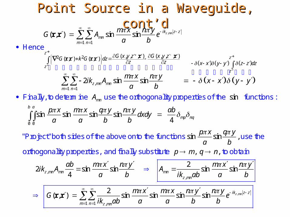
Point Source in a Waveguide, cont’dPoint Source in a Waveguide, cont’d
,
1 1
,1 1
2 2 ( , , ; ) ( , , ; )( , ) ( , )
( , ) sin sin
2 sin sin
z mnik z zmn
m n
z mn mnm n
z
z
G x y z G x y zG k G dzz z x x y y
m x n yG A e
a b
m x n yik A x x y y
a b
r rr r r r
r r
Hence
0 0
sin
sin sin sin sin4
"
mn
b a
mp nq
z
z
z z dz
A
p x m x q y n y abdxdy
a a b b
Finally, to determine use the orthogonality properties of the functions :
Project" both sides of the above onto the
,,
,
sin sin ,
, ,
22 sin sin sin sin
4
2( , ) sin sin sin
z mn mn mnz mn
z mn
p x q y
a bp m q n
ab m x n y m x n yik A A
a b ik ab a b
m x m x nG
ik ab a a
r r
functions use the
orthogonality properties, and finally substitute to obtain
,
1 1
sin z mnik z z
m n
y n ye
b b

2D Sources 2D Sources
( ) ( ) ( )
( ) ( ), 0
( ), 0
2
( ) ( )S
x x y y
dS dxdy
r r
r r r r
or
o
A two - dimensional (no - variation) "point" source
is actually a with unit line source density :
z
line source
( )
1,
0,
d d
S
S
S xy
r r
r
r
r
It is often convenient to treat the integration over in the -plane as a
integration over, say, a circular cylinder of and radius
volume unit height
.r centered about the point
ˆ ˆx y r x y(Reminder : In 2D, )
1[m]x
z
y
r
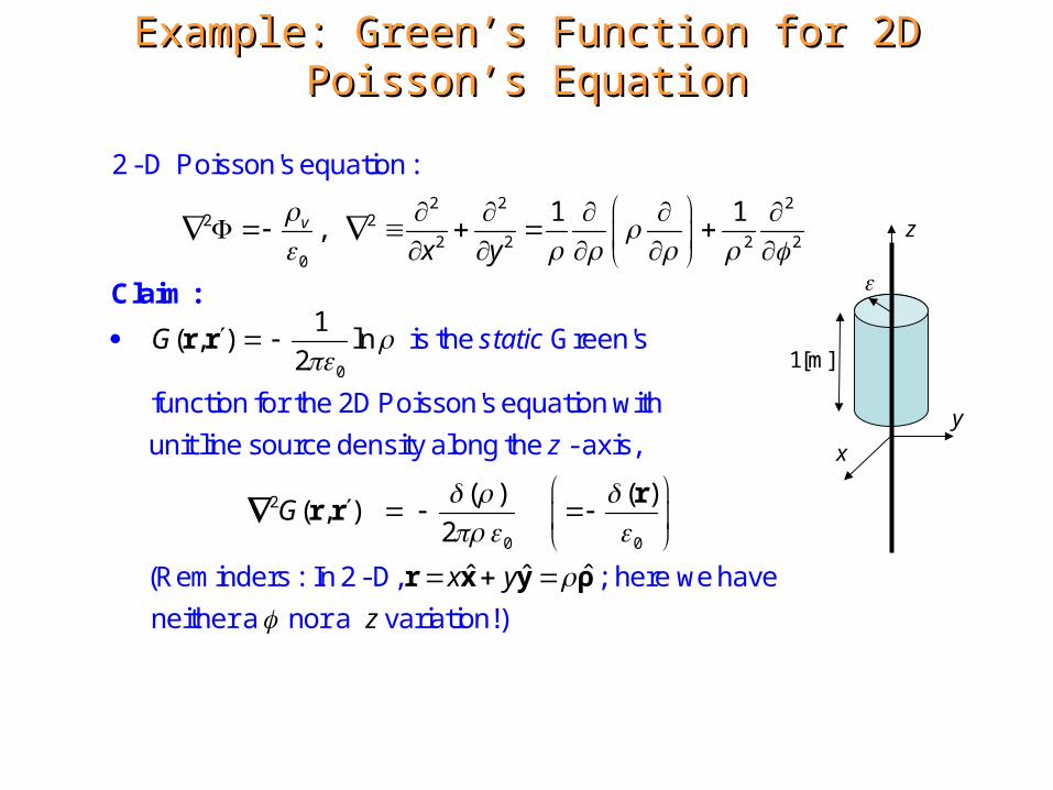
Example: Green’s Function for 2D Poisson’s Example: Green’s Function for 2D Poisson’s EquationEquation
2 2 22 2
2 2 2 20
0
1 1,
1( , ) ln
2
:
v
x y
G
r r
2 - D Poisson's equation
is the Green's
function for the 2D Poisson's equation with
unit line source density alon
Claim:
static
2
0 0
( ) ( )( , )
2
ˆˆ ˆ
G
x y
z
rr r
r x y ρ
g the - axis,
(Reminders : In 2 - D, ; here we have
neither a nor a variation!)
z
1[m]
y
x
z

““Proof” of Claim Proof” of Claim
0
( , )
1 1 1
2
G
d dG d
d d d
r r is a solution of the homogeneous Poisson (i.e., Laplace's) equation,
0
2
00, 0
2
0
0
( )( , )
2V
G dV
r r
,
the singularity at actually generates a delta function at
in Poisson's equation!
We must also show that
0
2
1
00 0
1
0.
d dz
V
when the integration domain is the unit height cylinder of radius
centered about the point Since the result of the integration
must be independent of , it suffices to c
1
2
0 00 00 0
0
( ) 1lim ( , ) lim 2
2V
G dV d dz
r r
onsider the limi
t
1[m]
y
x
z
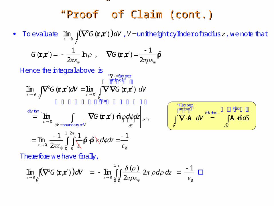
““Proof” of Claim (cont.)Proof” of Claim (cont.)
2
0
0 0
2
0 0
lim ( , )
1 1ˆ( , ) ln , ( , )
2 2
lim ( , ) lim ( , )
V
V
G dV V
G G
G dV G
r r
r r r r ρ
r r r r
" f
To evaluate , unit height cylinder of radius , we note that
Hence th
e integral above is
0
00
ˆlim ( , )
1 1lim
2
V
V V dS
dV
G d dz
r r n
lux per unit vol. "
Flux
div thm.
boundary of
ˆ ˆ ρ ρ
1 2
00 0
12
0 00 00 0
1
( ) 1lim ( , ) lim 2
2V
d dz
G dV d dz
r r
Therefore we have finally,
ˆV V
dV dS
A A n
" Flux per Flux unit vol. "
div thm.
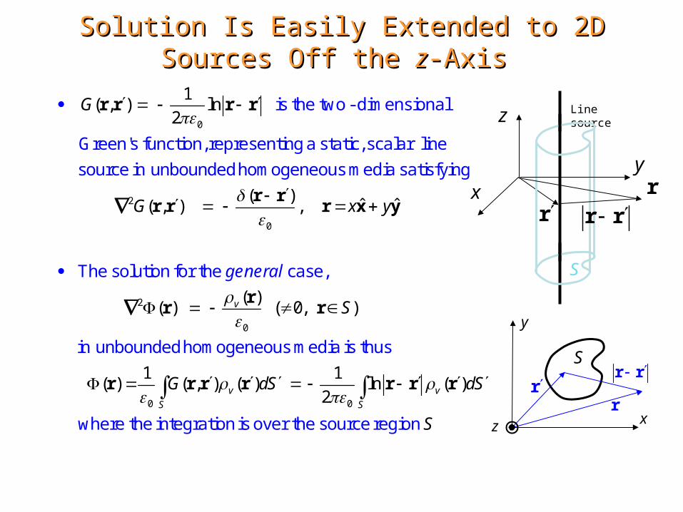
Solution Is Easily Extended to 2D Sources Off Solution Is Easily Extended to 2D Sources Off the the zz-Axis -Axis
0
2
0
1( , ) ln
2
( )ˆ ˆ( , ) ,
G
G x y
r r r r
r rr r r x y
is the two - dimensional
Green's function, representing a static, scalar line
source in unbounded homogeneous medi
a satisfying
The solution
for
2
0
0 0
( )( ) ( 0, )
1 1( ) ( , ) ( ) ln ( )
2
v
v v
S S
S
G dS dS
S
rr r
r r r r r r r
the case,
in unbounded homogeneous media is thus
where the integration is over the source region
general
x
r r
y
rr
S
z
x
z
y
rr
Line source
r r
S

Example: Green’s Function for 2D Wave EquationExample: Green’s Function for 2D Wave Equation
(2)0
2 2
( )( , )
4
( )( , ) ( , ) ( )
2
H kG
i
G k G
r r
r r r r r
is the
Green's function for the 2D wave equation
with unit line source density along the - axis,
and a harmonic tim
outgoing - wave
z
Claim:
(2)0
2
.
ˆˆ ˆ
( )
10
i te
x y
z
H k
d dyk y
d d
r x y ρ
e variation of the form
(Reminders : In 2D, ; here we have
neither a nor a variation!)
The solution of Bessel's equation,
, which is singular at 0, actually
generates a delta function there!
1[m]
y
x
z

““Proof” of Claim Proof” of Claim
2 2
(2)0
( ) 0, 0 ,
( , ) ( , ) 0, 0,
( )( , )
4
0
G k G
H kG
i
n
r r r r
r r
Since we must have
But this is indeed the case since
is an outgoing solution of the 2D wave equation
(note since there is no - variatio
1
2 2
0 0
( )( , ) ( , ) 2 1
2
0.
V
G k G dV d dz
V
r r r r
n))
We must next show that
when the integration domain is the unit height cylinder of radius
centered about the point Since the result of t
0 he integration
must be independent of , it suffices to consider the limit
1[m]
y
x
z

““Proof” of Claim (cont.)Proof” of Claim (cont.)
2 2
0lim ( , ) ( , )
0V
G k G dV V
r r r r
Evaluate , unit height cylinder of radius
Since we are integrating over a region near the origin , we may use
small argument approximations to the Hankel functi
0 0
2
0 0
21 ln
( ) ( ) 12ˆ( , ) , ( , )
4 4 2
lim ( , ) lim ( , ) limV V
ki
J k iN kG G
i i
G dV G dV
r r r r ρ
r r r r
" Flux per unit vol. "
div thm.
on,
Hence the first integral above is
0
1 2
00 0
1 202 2
0 00 0 0
2 2
00
ˆ( , )
1ˆ ˆlim 1
2
lnlim ( , ) lim
2
lim ln 0 ( , )
V V
V
G dS
d dz
k G dV k d d dz
k G
r r n
ρ ρ
r r
r r
Flux
boundary of
whereas the second i
s
2 ( , ) 1,V
k G dV V r r r
ˆV V
dV dS
A A n
" Flux per Flux unit vol. "
div thm.
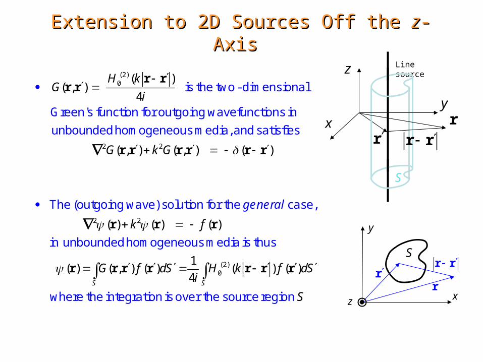
Extension to 2D Sources Off the Extension to 2D Sources Off the zz-Axis -Axis
(2)0
2 2
( )( , )
4
( , ) ( , ) ( )
is the two - dimensional
Green's function for outgoing wavefunctions in
unbounded homogeneous media, and satisfies
The (outgoing wave) solution
f
H kG
i
G k G
r rr r
r r r r r r
2 2
(2)0
( ) ( ) ( )
1( ) ( , ) ( ) ( ) ( )
4
or the case,
in unbounded homogeneous media is thus
where the integration is over the source region S S
k f
G f dS H k f dSi
S
r r r
r r r r r r r
general
x
r r
y
rr
S
z
x
z
y
rr
Line source
r r
S
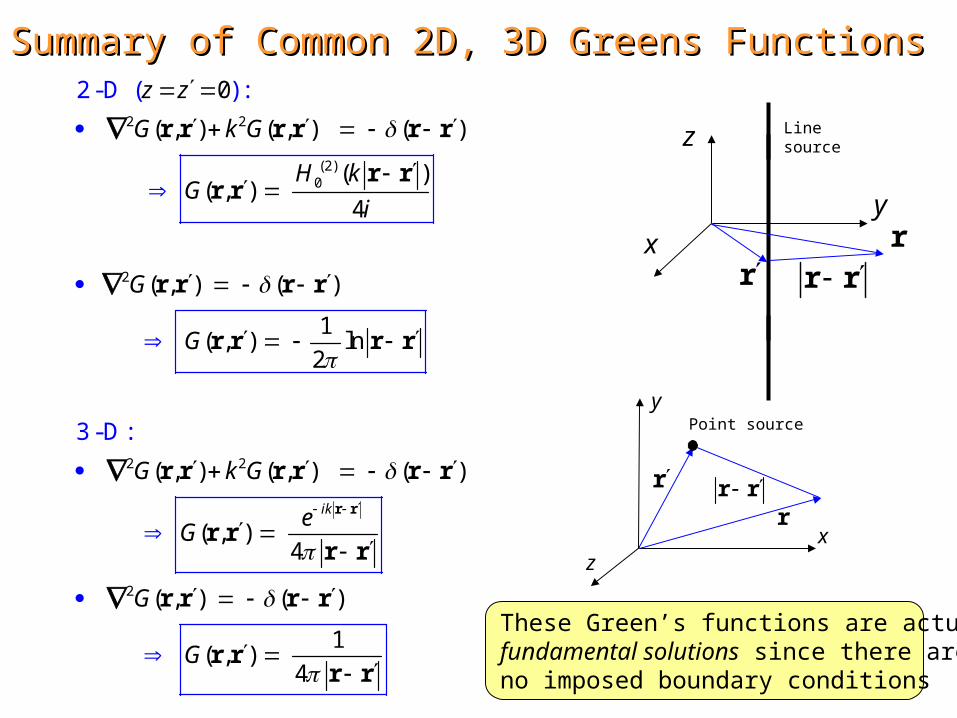
Summary of Common 2D, 3D Greens FunctionsSummary of Common 2D, 3D Greens Functions
2 2
(2)0
2
2 2
2
0
( , ) ( , ) ( )
( )( , )
4
( , ) ( )
1( , ) ln
2
( , ) ( , ) ( )
( , )4
( ,
( )
) ( )
1( , )
4
ik
z z
G k G
H kG
i
G
G
G k G
eG
G
G
r r
r r r r r r
r rr r
r r r r
r r r r
r r r r r r
r rr r
r r r r
r rr r
2-D :
3 -D :
x
z
y
rr
Line source
r r
x
r r
y
r
r
z
Point source
These Green’s functions are actually fundamental solutions since there areno imposed boundary conditions

Line Source Illumination of a Circular Cylinder Line Source Illumination of a Circular Cylinder
x
y
a
Line source
(2)0inc ( )
ˆ( ) ,4
z
H k
i
r r
r r x
A line source illuminates a circular cylinder;
both are parallel to the -axis. Hence the
incident field is
The field satisfies the Dirichlet boundary
condition
totalinc sca
2 sca 2 sca
( ) ( ) ( ) 0
( ) ( ) 0.
a
k
r r r
r r
at
on the cylinder surface.
The scattered field is source - free and hence is an
outgoing solution to
In cylindrical coordinates it must have th r
e fo
sca (2)
0
( ) ( ) inn n
n
a H k e
r
m

The Addition TheoremThe Addition Theoreminc
(2) ( )
(2)0
( )
0.
( ) ( ) ,
( )
(
inn n
n
n
x y
H k J k e
H k
J k
r
r r
We need an expansion for in terms of cylindrical wavefunctions
about Such an expansion is provided by the addition theorem
(2) ( )) ( ) ,
0.
inn
n
H k e
x
where is the angular position of the line source relative to the -axis. For
our problem,
The addition theorem is analogous to the Laurent expansion abo
1
0
1
0
,1
,
n n
n
n n
n
z z
z z z z
z zz z z z
ut the origin
of a simple pole at :
x
y
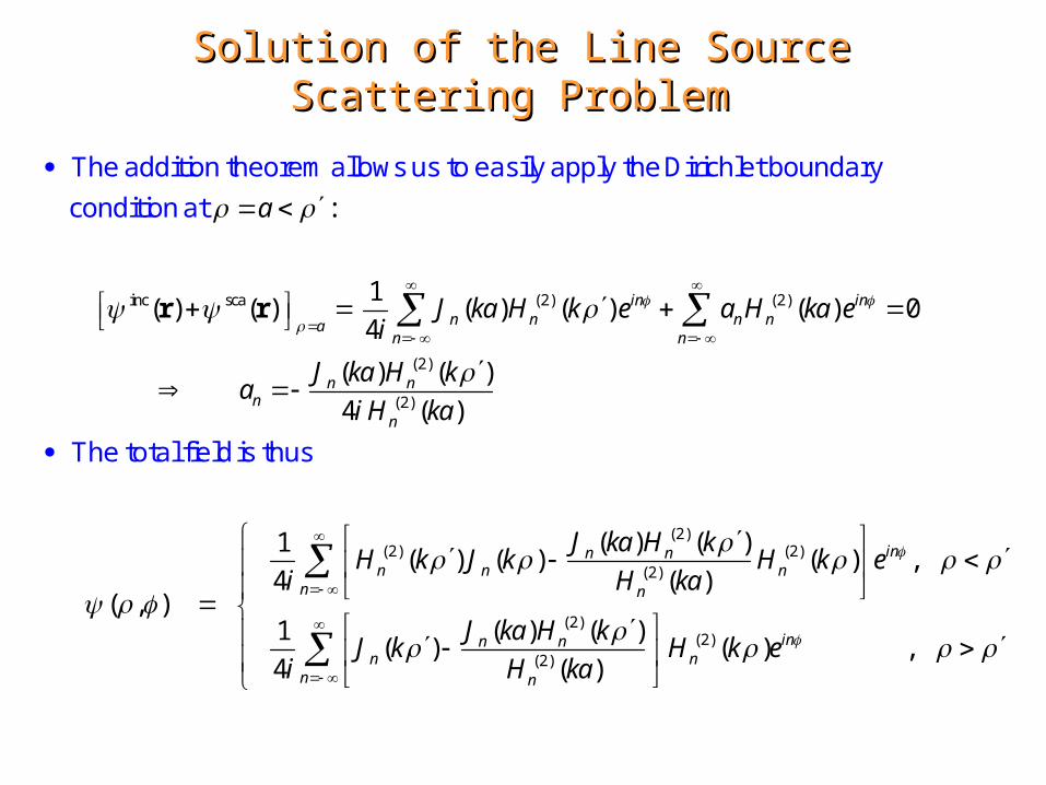
Solution of the Line Source Scattering Problem Solution of the Line Source Scattering Problem
inc sca (2) (2)
(2)
(2)
:
1( ) ( ) ( ) ( ) ( ) 0
4
( ) ( )
4 (
in inn n n na
n n
n nn
n
a
J ka H k e a H ka ei
J ka H ka
i H k
r r
The addition theorem allows us to easily apply the Dirichlet boundary
condition at
(2)(2) (2)
(2)
(2)(2)
(2)
)
( ) ( )1( ) ( ) ( ) ,
4 ( )( , )
( ) ( )1( ) ( ) ,
4 ( )
inn nn n n
n n
inn nn n
n n
a
J ka H kH k J k H k e
i H ka
J ka H kJ k H k e
i H ka
The total field is thus

Interpretation as a Green’s FunctionInterpretation as a Green’s Function
The source is a unit strength line source
We can obtain the result for a line source
the x -axis by simply replacing by
Hence a Green's function for the cylinder scattering problem is
off
(2)(2) (2)
(2)
(2)(2)
(2)
(2)0
( ) ( )1( ) ( ) ( ) ,
4 ( )( , )
( ) ( )1( ) ( ) ,
4 ( )
( )
4fundamentalsolution
inn nn n n
n n
inn nn n
n n
J ka H kH k J k H k e
i H kaG
J ka H kJ k H k e
i H ka
H k
i
r r
r r
(2)
(2)(2)
( ) ( )1( )
4 ( )homogeneous solution
inn nn
n n
J ka H kH k e
i H ka
Line source
x
y
a