D-A127 928 FAULT DIAGNOSIS OF NONLI NEAR ANALOG CIRCUITS VOLUME IV 1/1AN ISOLATION ALOOR..(U) PURDUE UNIV LAFAYETTE IN SCHOOLOF ELECTRICAL ENGINEERING Y S ELCHERIF ET AL. APR 82

UCASIFIED NB8184-81-K-0323 F/G 9/5 N

MEMMEMEMEBMllIhlBhhBBhhBBiEEhhhhhhhhhhhhIIIIIflllffflffllf

.- 2.2

- . . -

.0.

II ,

36

- S!I,,..[ 5 1.4 1.8

MICROCOPY RESOLUTION TEST CHART

ATONAL BUREAU Of STANOAROS-963-A

PV.

F'-

*4:.;

a7

.1 ;.p' Jill

"1.. 71

CD

C.> A11983

7ths work we mupported by Offie of Naval Research, aCostract No. Nuwl44l-K0323.

82 04 19 9

.. .

FAULT DIAGNOSIS OF NONLINEAR ANALOG CIRCUITS

VOLUME V

AN ISOLATION ALGORITHM FORTHE ANALOG FAULT DICTIONARY

Y. S. ElcherifP. M. Lin

April 1983

School of Electrical Engineering

Purdue UniversityWest Lafayette, Indiana 47907

This work was supported by Office of Naval Research,Contract No. N00014-81-K-0323.

di Acir '4 ; -iS : 1,* . bu . i : i -. ..

LhI

il

.ECUnITY CLASSIFICATION OF THIS PAGE (When fate Entered)

READ INSTRUCTIONSREPORT DOCUMENTATION PAGE BEFORE COMPLETING FORM1. REPORT NUMBER 12. GOVT ACCESSION NO. 3. RECIPIENT'S CATALOG NUMBER!AkI4 1 a-o4. TITLE (and Subtitle) S. TYPE OF REPORT & PERIOD COVERED

Fault Diagnosis of Nonlinear Analog Circuits, Volume* IV, An Isolation Algorithm for the Analog Fault

Dictionary. G. PERFORMING ORG. REPORT NUMBER

7. AUTHOR(&) 8. CONTRACT OR GRANT NUMBER(&)

Y. S. Elcherif , P. M. Lin N00014-81-K-0323

9. PERFORMING ORGANIZATION NAME AND ADDRESS 10. PROGRAM ELEMENT, PROJECT, TASK

Purdue UniversitySchool of Electrical EngineeringWest Lafayette, Indiana 47097

11. CONTROLLING OFFICE NAME AND ADDRESS 12. REPORT DATE

Office of Naval Research April 1983Arlington, Virginia 13. NUMBER OF PAGES

5314. MONITORING AGENCY NAME & ADDRESS(if different from Control'lng Office) 15. SECURITY CLASS. (of this report)

SAMEUnclassif iedISa. DECL ASSI F1 CATION/ DOWNGRADING

SCHEDULE

" f16. DISTRIBUTION STATEMENT (of this Report)

Approved for Public Release

17. DISTRIBUTION STATEMENT (of the abstract entered In Riok 20, If different from Report)

SAME

IS. SUPPLEMENTARY NOTES

NONE

19. KEY WORDS (Continue on reverse side if necesary and Identily by block number)

Fault DiagnosisFault Dictionary

20. ABSTRACT (Continue on reveree aide if necessary and Identify by block nuober A new approach forfault location in an analog fault dictionary has been adopted on the basis ofquantizing circuit reponses. The possibility of quantization is offered by faultshaving nearly the same effect on some test measurements. This produces multi-valued logic responses which can be manipulated logically to obtain decision rulesfor fault location. A logical isolation algorithm has been introduced to form adictionary for hard fault diagnosis using d.c. voltage measurements. The dictionaryconsists of tables containing voltage ranges of quantized response and

DD jAN73 1473 EDITION OF I NOV 65 S OBSOLETE

S/N JAN2L 3 144. 6SECURITY CLASSIFICATION OF THIS PAGE (When Data Entered

SECURITY CLASSIFICATION OF TIS PAGE (When Date Entered)

numerical codes identifying different faults in the dictionary. Thetest measurements chosen by the algorithm are free from redundancyand provide the maximum fault isolation capability of all initially chosenmeansurements. The algorithm can be easily implemented with someextra software added to the circuit simulator used in fault simulation.Hardware implementation of a logical isolation ATE is simple and efficientcompared to a least squares based dictionary. The algorithm has beenextended to handle multiple test input conditions.

Ava

I

S CD

SEUITLAS.IAIO• .... A EI*,. at nttd

TABLE OF CONTENTS

Abstract................................................................................1.

1. Introduction ............................................................................ 2

2. An overview on the analog fault dictionary......................................... 3

2.1 Generation of the analog fault dictionary...................................... 32.2 Fault location based on minimum sum of squares............................ 6

3. A new algorithm........................................................................ 13

3.1 Forming ambiguity sets .......................................................... 133.2 Fault isolation..................................................................... 153.3 Generation of fault codes......................................................... 163.4 Fault location...................................................................... 28

4. Binary representation of the algorithm.............................................. 33

4.1 Ambiguity set-fault truth table.................................................. 334.2 Minimality of the realization..................................................... 384.3 Fault isolation..................................................................... 384.4 Fault location...................................................................... 44

5. Isolation with multiple test input conditions ....................................... 46

6. Conclusions and suggestions for future research.................................... 50

*References ................................................................................ 53

ABSTRACT

A new approach for fault location in an analog fault dictionary has been adoptedon the basis of quantizing circuit responses. The possibility of quantization is offeredby faults having nearly the same effect on some test measurements. This produces mul-tivalued logic responses which can be manipulated logically to obtain decision rules forfault location. A logical isolation algorithm has been introduced to form a dictionaryfor hard fault diagnosis using d.c. voltage measurements. The dictionary consists oftables containing voltage ranges of quantized responses and numerical codes identifyingdifferent faults in the dictionary. The test measurements chosen by the algorithm are

*" free from redundancy and provide the maximum fault isolation capability of all initially. chosen measurements. The algorithm can be easily implemented with some extra" software added to the circuit simulator used in fault simulation. Hardware implemen-

tation of a logical isolation ATE is simple and efficient compared to a least squaresbased dictionary. The algorithm has been extended to handle multiple test input con-ditions.

--. - t

-.

['

.A -2-

1. INTRODUCTIONThe problem of analog fault diagnosis of electronic circuits has been addressed by

many researchers from different view points [1]. Within the frame of general testing*: strategy of electronic equipments, we are here concerned with fault location in malfunc-

tioning analog circuit boards. The term "testing strategy" roughly means the pro-cedure followed in testing different modules in modularly structured equipments. Forexample in case of complete failure, the first module to be checked is the power supplymodule, which is more likely to be the cause of trouble than any other module, based

* on trouble shooting experience and fault history. Other types of malfunction may beindicative of the failing module, e.g. if the picture is fading in a monitoring system, themost likely cause may be the video processing unit. In the worst case of a completelyunknown source of trouble, automatic fault diagnosis may be applied sequentially to all

* modules, in which case a fast enough technique has to be available in order to achievethe job in a reasonably short time.

This discussion has been meant to give some insight into practical considerationsin trouble shooting which are in direct connection with our approach in this report.The figure of merit which we have planned to achieve is the speed of diagnosis withoutdegrading its reliability, with the purpose of handling a large number of circuits in ashort time.

Looking at the different fault diagnosis approaches available in literature [2] we• can note two main categories in which every method can approximately be included.* These are the "simulation after test" and "simulation before test" approaches. Simula-

tion after test, sometimes called component simulation [31, is intended to solve for com-ponent values from knowledge of some network functions (voltages, currents orimpedances) measured at accessible network terminals. This is done by solving the net-work equations in frequency or time domain as derived by KCL, KVL and componentcharacteristics. This implies that all simulations have to be done after actual testing.Adding to this the complexity of the equations to be solved, it turns out that powerfulcomputing facility and long computing time are needed which does not serve the pur-pose of our work. Naturally we have adopted the other approach in order to minimizethe computations needed after testing or completely eliminate them if possible.

This, often called fault dictionary approach, is in its essence an automatic meanstl for replacing human logic in troubleshooting which depends on counting all or most

possibilities of likely faults until the true fault is located. This requires solving the net-work equations under all fault cases, which may be caused by single or multiple com-ponent failure, and storing the computed response or any network function which willbe taken as a criterion to be compared against measured values after testing. The cri-teria employed could be voltage, current, etc. The problem that obviously faces this

1

-3-

technique is the multitude of faults which must be considered in simulation. However,it has been reported [4] that catastrophic faults (open and short-circuits), also calledhard faults, constitute more than 80 percent of encountered faults, which suggests that

*simulating only these faults, one can locate a good percentage of faults using only anefficient fault dictionary. This saves the effort needed in component simulation every

* •time a diagnosis is needed. With only open and short circuit faults considered, it turnsout that only d.c. analysis of the network is needed, which makes fault simulation even

- simpler.

* •Organization of the report:

The next section explains the general procedure for fault dictionary set up andpresents a least squares based algorithm for fault isolation in the dictionary. Section 3presents a new algorithm for fault isolation based on quantizing circuit responses. The

:. possibility of quantization is offered by faults having nearly the same effect on some

test measurements. The algorithm is built around the digital representation of theresponses and is implemented by logical manipulation of the quantized responses. In

section 4, the logical binary equivalent form of the algorithm is discussed. This offers asolution to the problem of minimizing the number of test measurements. Importantissues in the cost of implementing the algorithm and building a logical isolation-based

*ATE are discussed in the context of binary representation of the algorithm. In section5, the algorithm is extended to handle multiple test input conditions. The use of

* different test inputs is subject to the insufficiency of test measurements under normaloperating input conditions. Section 6 contains conclusions and suggestions for furtherresearch.

2. AN OVERVIEW ON THE ANALOG FAULT DICTIONARY

* 2.1 Generation of the AL&Jog Fault DictionaryThe generation of analog fault dictionaries is in fact an iterative process with two

* degrees of freedom which represent the possibilities of varying the input excitation andselecting the responses to be measured as shown in Fig. 2.1. The selection of the fault

* .list is essentially associated with the original design of the unit under test (UUT). How-ever, an experienced person can replace the designer in selecting the faults which are

9 likely to happen. The selection of the measurable responses is influenced by theI. required level of isolation and the economy of the testing procedure insofar as the

number of measurements is concerned. The input stimuli considered here are d.c. vol-tage or current sources which may be different from the nominal operating sources andapplied at judiciously selected points in the network. The reason behind using any

* additional input stimulus is the possible insufficiency of the selected measurableresponses to achieve the required level of isolation. Applying the additional input, it is

-4-

Fault Test Testconditions inputs Measurements

Circuitd t Circuit Simulator[ description -

Eliminateredundant measurements

Set up the dictionaryfor the ATE

Figure 2.1 Flow chart of the general procedure forgenerating an analog fault dictionary.

'|

I-

hoped that some of the faults, which have not. been isolated with nominal sources, willbe propagated to some of the accessible terminals at which responses are measured.

Once the required faults are satisfactorily isolated, the software and data of theautomatic test equipment (ATE) have to be prepared. In its basic form, the ATE datais the computed response values which have been found enough for isolation. Othernecessary software support depends on how faults will be located in the dictionary aftertesting, or in other words the decision rule employed in fault location. The capabilitiesof the circuit simulator are determined by the requirements of the type of analysis to beused. Some circuit analysis programs may not allow direct simulation of open andshort circuits without changing the program input in which case, a method for simulat-

ing them has to be tailored to suit the program and the method of analysis. Therepeated solution of the network under all fault conditions may be time consuming.For this reason, specially designed methods for hard fault simulation have been sug-gested [5], [6] which do not require solving the original network every time a fault issimulated. In all the discussions to come we will assume that the responses to be usedin isolation have been computed already, regardless of the method used in computingthem. More specifically, we will focus on d.c. node voltages because of their easy meas-

* •urement.At this point it is important to make clear the difference between two problems

which are defined below.

1. Fault isolation:This means finding a set of tests or measurements that enable us to recognize all

faults if any one of them happens. Before dealing with the problem, it may be instruc-tive to note some of the inherent features of analog respoDses which govern any faultisolation study:

1. Unlike digital functions, analog voltages span a continuous range of values where it

* - may seem that the exact value of the voltage is the quantity of interest. However,the evident variability of any response as a result of the components' statisticalvariation makes it necessary to talk about ranges of voltages instead of their exactvalues.

2. The network topology imposes some restrictions on the sensitivity of responses4 measured at accessible terminals to some of the faults, at least under normal

operating conditions. In other words, not every fault will affect every terminal.This will result in having groups of faults having almost the same effect on somenode voltages. We reft -eA to t' earlier as the insufficiency of some terminalmeasurements to reveal th- ,tuai fault. Rather we will have ambiguous cases andambiguity sets of faults which have to be further analyzed and broken down totheir elementary constituents using different measurements. This process is known

I

in reliability studies as a fault tree [7].

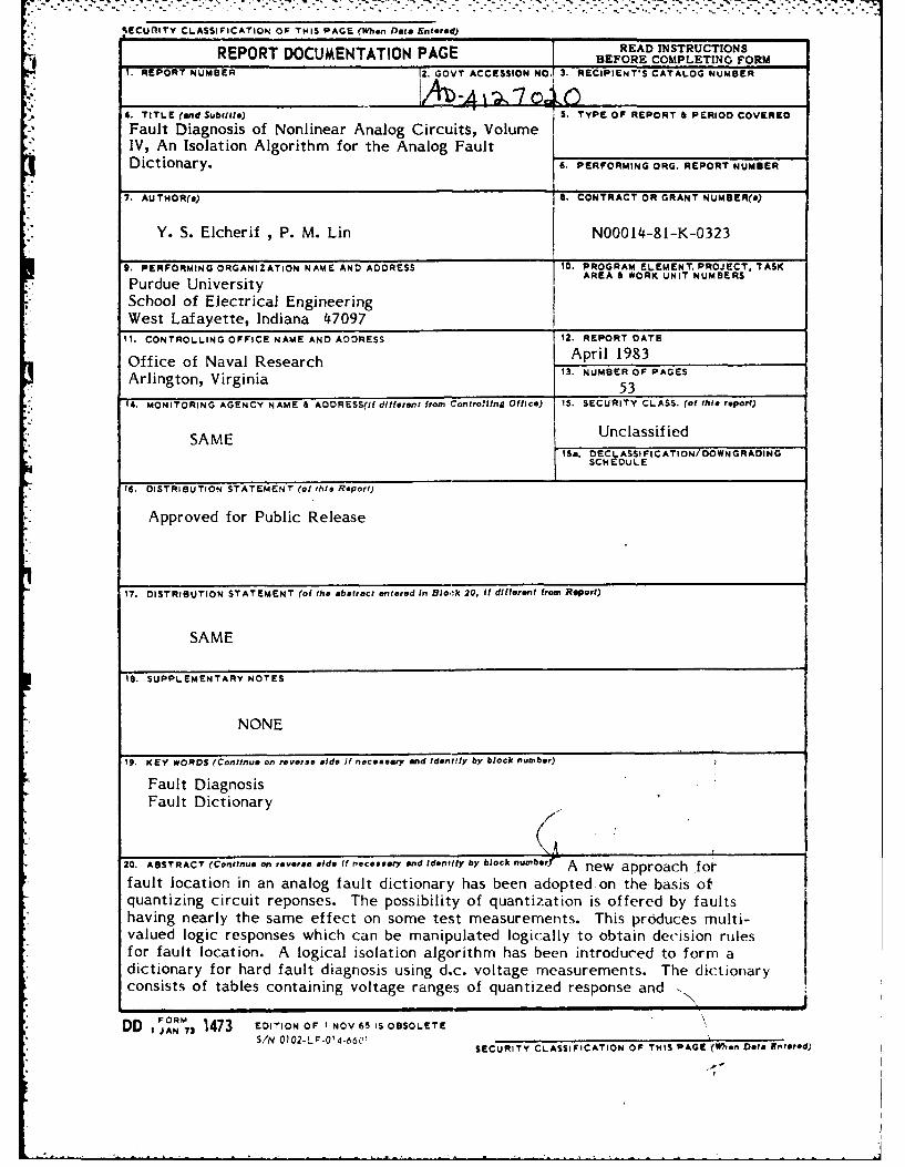
2. Fault Location:By fault location, we mean the procedure to be followed after testing to locate the

actual fault among all faults in the dictionary. The problem may be better viewed inthe space of measurements. Suppose that (V,V2...v E V .R n is the set of measurementsnecessary for location of any fault in the set {ff2... fm}. The result of simulation is mpoints in RI representing the m faults. Given the actual measurement represented bya point in i"n it is required to find a point of the m simulations which is nearest to theactual measurement. The difficulty of the problem arises from the fact that the actualmeasurement will never coincide with any of the simulations because of the statisticalvariation of the components in the network and consequently of the node voltages.

This problem is obviously a pattern classification problem where every class is only asingle point in IRn and the pattern to be classified is also a single point. This is called"the nearest neighbor" problem. The nature of the problem as presented here may notalways be explicitly stated in literature dealing with fault dictionary, however we viewthe decision rule for fault location in a dictionary as a pattern classifier which is obvi-ous in a linguistic sense. Classification or finding the nearest neighbor is done on an

*] optimal basis which may or may not take into consideration the statistical properties ofthe pattern to be classified. Optimality is usually sought by defining a distance meas-

ure which is thought to be best representative of the properties of the space dealt with.For example, in IRn the second order Euclidean norm is often considered as the

*optimality criterion.

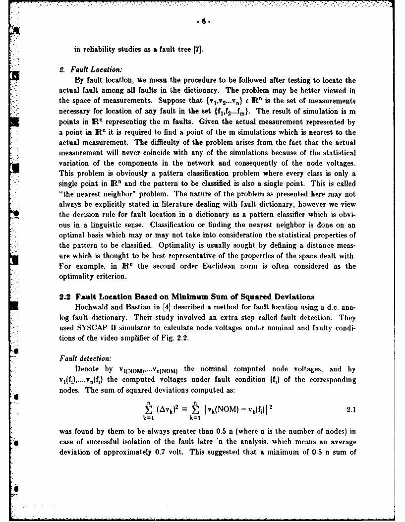
2.2 Fault Location Based on Minimum Sum of Squared DeviationsHochwald and Bastian in 14] described a method for fault location using a d.c. ana-

log fault dictionary. Their study involved an extra step called fault detection. Theyused SYSCAP II simulator to calculate node voltages und, r nominal and faulty condi-tions of the video amplifier of Fig. 2.2.

Fault detection:Denote by VI(NOM),...vn(NOM) the nominal computed node voltages, and by

v1 (f),...,Vn(f1 ) the computed voltages under fault condition (fi) of the corresponding

nodes. The sum of squared deviations computed as:n n

(Avkj2 - I Vk(NOM) - vk(fi)I 2 2.1k=! k=1

was found by them to be always greater than 0.5 n (where n is the number of nodes) in" case of successful isolation of the fault later "n the analysis, which means an average

deviation of approximately 0.7 volt. This suggested that a minimum of 0.5 n sum of

8 -7-

044

- 011

, 0"*8alas

0a""

9. 0850

so) 1. 'I.4 I zw4.2 e -3 LI -- -. 'v J z

* *04. 6,013

DZI L32 t A 12DI

-S : D2

S. S . ,Z300O 2 - . I I a _

l985~ ~ .- 0I 4) 444O

)*2 ~ ~ ~ 03 V.~ 44 06 32 @s 00

9 2 ., 43 -S7 aig 1

Is I.sS L4 I4 PS, ,~ 4

t2210 IS 0

O-s

F ig. 2.2. Video amplifier discussed in sections 2.2 and S.

-8-

squared deviations is required in order to detect the fault. The only degree of freedomallowed to achieve this for a particular set of arbitrarily chosen test nodes is varyingthe input stimuli as shown in Fig. 2.3 taken from 14).

Forming ambiguity sets:The :0.7 volt average deviation was taken as the range of variation for nominal

and simulated faulty voltages. The possibility of overlapping ranges is there. However

the ranges themselves are not needed once the faults belonging to every ambiguity setare identified. A problem may exist if some fault exists in the overlap area betweentwo adjacent ranges. However, this was not mentioned, and it seems that human inter-vention had to be used to select the ranges in such a way to prevent this situation.

The result is listed in Table 2.1. The notable thing about this table is the exclusion ofthe nominal ambiguity set on the basis of the 0.5 n detection criterion. It was believedthat faults producing node voltages in the nominal range make the measurement of

these voltages useless. We believe that this is a loss of information that caused someunnecessary effort later on during the isolation process. The use of nominal ambiguitysets will prove to be useful in the new algorithm to be explained in the next sections.

Fault isolation:

At this point, it has to be assured that the chosen set of nodes is capable of uniquecharacterization of all faults. It is also important to discover if there are unnecessarymeasurements which do not help in isolation. The ground rules stated by the authorsto check the above two features are:

1. Any ambiguity set which has a single fault within it, uniquely defines that fault atthat test node.

2. Ambiguity sets whose intersection or symmetric difference result in a single fault,also uniquely identify the fault.

Indeed the symmetric difference between two sets (of two different node) must be

the intersection of one of them with the nominal ambiguity set of the other node whichhas been omitted.

Starting with the ten nodes in Table 2.1 and using the above mentioned rules it4 was possible to find a subset of only five nodes (11, 8, 5, 2 and 16) which were sufficient

for unique isolation of all faults except the pair 10 and 12. This means isolating 95 per-

cent of the listed 20 faults.

. .. . .. . .

-9-

ENGINEER

NETWORK FAULTDESCRIPTION DEFINITION

SYSCAP B ~ INPUTELMNTSTIMULI UNNECESSARY

SIMULATOR TEST~iO

DC NODAL SET-UPVOLTAGES AND FAULT DICTIONARY

COMPONENT AMBIQUITY GROUPOVERSTRESSES SECONDARY OVERSTRESSES

ADEQUTELYATE SO-FTWARE

YES

YE

Figure 2.3 Flow chart for generating a least square based fault dictionaryusing SYSCAP Hi circuit simulator.

-10-

Table 2.1. Ambiguity sets of faults simulated in the video amplifier of fig. 2.2. Thenominal set contains the rest of the 20 faults.

Node Input Set No. 1 2 3 4 5

* 11 +30 3,6,7,15,19 nominal-30 2 5 13 14 nominal

8 +30 3 7 15 16 nominal-30 2,4,5,13 nominal

5 +30 3,6,7,15 nominal-30 2,4,5,13 9 17 18 nominal

2 +30 3,6,7,15 19 20 nominal-30 2,4,5,8,9,13,17 nominal

27 +30 3,6,7,15,19 nominal-30 2,4,5,8,9,13,17 nominal

26 +30 3,6,7,15,19 nominal-30 2,4,5,8,9,13,17 nominal

33 4-30 3,6,7,15,19 nominal-30 2,4,5,8,9,15,17 nominal

36 +30 nominal-30 nominal

18 +30 nominal-30 nominal

16 +30 3,6,7,10,12,15,19 nominal-30 2,4,5,8,9,15,17 11 nominal

Fault location:The fault dictionary then consists of the values of the simulated voltages of the

selected nodes for both inputs under all fault conditions which results in (5x2x19) 190* real numbers. To illustrate the use of the dictionary three faults were simulated on the

circuit board and measurements of the five test nodes were taken. The procedure to befollowed afterwards is:

1. Finding the difference between simulation results and measured values.2. Finding the sum of the squares of these differences under both input conditions.

~-11 -

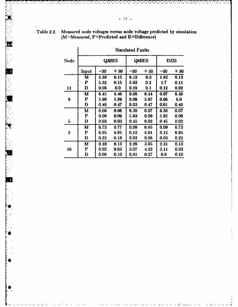
Table 2.2. Measured node voltages versus node voltage predicted by simulation(M=Measured, P-Predicted and D-Difference)

Simulated Faults

Node Q3BES Q6BES DZIS

Input -30 +30 -30 +30 -30 +30M 5.38 0.15 6.12 0.3 1.82 0.13P 5.32 0.15 5.93 0.2 1.7 0.11

•I D 0.06 0.0 0.19 0.1 0.12 0.02M 6.45 6.46 0.06 6.44 0.07 6.46

8 P 5.99 5.99 0.09 5.97 0.06 6.0D 0.46 0.47 0.03 0.47 0.01 0.46

M 0.06 0.06 6.38 0.07 6.38 0.07P 0.09 0.09 5.93 0.09 5.92 0.09

5 D 0.03 0.03 0.45 0.02 0.45 0.02M 6.73 6.77 0.09 6.85 0.09 6.73

2 P 6.05 6.95 0.12 6.91 0.12 6.95D 0.22 0.18 0.03 0.06 0.03 0.22M 0.10 0.13 2.26 3.95 2.31 0.13

16 P 0.02 0.03 3.07 4.22 3.11 0.03D 0.08 0.10 0.81 0.27 0.8 0.10

0

0

-12-

Table 2.3. Sum of the squared deviations for three hardware induced voltages.

Induced Faults

Fault 4 Q3BES Fault 10 QOBES Fault 4 DZIS

Fault No. -30 + 30 Total +30 -30 Total +30 -30 Total

1 130 0.3 130 1 16 17 18 0.3 18

2 29 0.3 29 163 16 179 129 0.3 129

3 128 171 299 0.9 154 155 18 171 189

4 0.3 0.3 0.6 128 16 144 139 0.3 139

5 7 0.3 7 132 16 148 167 0.3 167

6 128 103 231 0.9 87 88 18 102 120

7 128 100 228 0.9 85 86 18 99 117

8 69 0.3 69 53 16 69 70 0.3 70

9 109 0.3 109 57 16 73 74 0.3 74

10 129 17 146 0.9 0.3 1.2 18 17 35

11 119 0.5 119 3 11 14 20 0.6 20

12 129 17 146 0.9 0.3 1.2 18 17 35

13 93 0.3 93 127 16 143 300 0.3 300

14 141 0.3 141 20 16 36 0.9 0.3 1.2

15 129 177 306 0.9 160 161 18 178 196

16 129 22 151 0.9 38 39 Is 22 40

17 264 0.3 264 126 16 142 143 0.3 143

18 96 0.3 96 23 16 39 40 0.3 40

19 129 86 215 0.9 68 69 18 86 104

20 129 19 148 0.9 35 36 18 18 36

-13-

3. Finding the smallest number in these sums.

The actual fault is expected to produce the smallest sum of boxes. The results of theabove three steps are shown in Tables 2.2 and 2.3 with the minimum sum of squares

"* ."enclosed in squares. The fault pair 10 and 12 which could not be isolated are seen to* give the same sum of squares.

3. A NEW ALGORITHMThe basis of the new algorithm is making full use of the ambiguity clusters of

faults which have almost the same effect on terminal measurements. The result is to*confine our interest only to the ranges of voltages occupied by measurements of a faulty

circuit instead of the whole continuum of values. This effectively transforms the prob-lem from analog to digital. However this digitization yields multivalued logicalresponse instead of the usual binary. It is easy to see that this can be furthertransformed to binary logic if every set of faults is treated as a binary variable. If theresponse lies within the range (vmin,vm.) a logical 1 is obtained. Otherwise it gives alogical zero. This is shown in Fig. 3.1. The isolation process can be looked at as a logi-

*cal realization problem whether it be in binary or multilevel form. We will first present"* the solution in the multilevel form for better clarity, then proceed to consider impor-

tant implications of the binary representation. The requirement of the realization prob-lem is to obtain a digital expression for every fault (as a digital function) in terms ofthe digital variables which are the ambiguity sets. A systematic fault tree generationwill be shown next, which simultaneously achieves the following:

* 1. Eliminate the redundancy in the test measurements.2. Find out the maximum isolation capability of the initially chosen set of measure-

ments.3. Generate the required logical expressions of the faults. These logical expressions

will form the required dictionary. The arrangement of the expressions in the dic-tionary will make the fault location task fairly easy and efficient. To prevent con-fusion, we should note here that the logical expression will be described often as"fault code". We will also use the word "set" sometimes instead of ambiguity set.

3.1 Forming Ambiguity SetsClassifying the faults into ambiguity sets depends on some tolerance of the node

voltages. In the example to follow in this section a tolerance of -0.7 volts is used. Thefaults are divided into ambiguity groups which cause the node voltage to be incorresponding ranges. Each range is centered around the voltage value due to some

6 fault called the center of the ambiguity set. Eventually, each node will producedifferent grouping of the faults depending on how the faults affect this particular node

0

-14 -

.8A

c n Q

r.4

(U

4a)o

L

rr-

2 (Y)

:- 15 -

voltage. Thus there will be several ambiguity sets of faults, or just one set, associatedwith each node. Since there is no priority given to any particular fault, the ambiguitysets of every node can be found from "the node" voltages under different fault condi-tions by the following procedure:

1. Start with the nominal case as the center of ambiguity set j, j I 1 (called nominalset).

2. Scan all faults. If any voltage is within A0.7 volt of the center voltage, include thecorresponding fault in the set j, j = 1.

3. When all faults are scanned, take the first fault which has not been included in aprevious set to be the center of the new set and let j = j+ 1. If every fault has beenincluded in some set stop.

4. Do the same as step 2 for the current set j. If an overlap occurs between the rangeof this set and any previous range, divide the overlap region into two halves. Anyvoltage in the overlap region will cause the corresponding fault to belong to the setwhose center is nearer. Go to step 3.

3.2 Fault IsolationGiven the ambiguity sets derived from the simulation results, the algorithm

proceeds as follows. Integer values are assigned to the ambiguity sets of every node in

the set of nodes {vi} N', where N, is the number of test nodes. The different nodes willgenerally possess different numbers of ambiguity sets. The iPh node has Li sets includ-ing the nominal ambiguity set (i.e. faults which do not cause deviation from the nomi-nal response).

A fault is characterized by being the single element contained in any set or theintersection of any number of sets of different nodes (since any fault belongs only to oneset of every node). Therefore, intersection operations will be performed. The object tobe achieved is to have a number of sets resulting from intersection which is equal to thenumber of faults Nf. In this case, all faults will be isolated since every set cannot con-tain more than one fault and in the same time every fault cannot be contained in morethan one set.

If all sets of all nodes are exhausted without achieving Nf nonempty intersections,the result will be the best degree of isolation that can be obtained with the available

* nodes. In this case, some sets resulting from intersection will still contain more thanone fault. These contents cannot be distinguished using only these nodes without addi-tional input stimuli.

If it happens after intersecting the sets of some node with the resulting sets of pre-vious intersections that the total number of sets is not increased, then no information isadded by this new node. This means that this node is redundant and has to beexcluded. This would imply that there is no redundancy in the set of nodes obtained

~- 16 -

after intersection, but it would not guarantee that the number of nodes is minimum,i.e. there is no subset of these nodes which could achieve the same degree of isolation,but there could be another set of other nodes, less in number, and same in isolation

capability. This depends on the sequence of nodes being intersected. However, to

approach the minimum number of nodes, one should give priority to nodes with higherisolation capability, which is in this case represented by a larger number of ambiguitysets.

The exact minimum number of nodes may not be of considerable practical impor-tance. The minimization problem will be presented later in the context of Booleanrepresentation of the isolation process. The solution to the problem, though known, istime consuming. The isolation process is illustrated in the fault tree diagram of Fig.3.2.

3.3 Generation of fault codes:The third goal of the algorithm which is generating the fault codes is done using a

"labeling technique" (after a well-known graph algorithmic notion [8]) which employsthe integer values assigned to the different logic levels (i.e. the different ambiguity sets).The method is basically describing every fault in terms of the sets in which this fault isa common member. This is done by identifying every set resulting from intersection bythe labels of the sets producing it, in proper order. After the last intersection step, wewill have an integer code characterizing every fault. The length of the code is equal tothe number of nodes. The implementation of this part requires a stack (an expandable

storage) which is updated after every intersection. This will be best illustrated throughthe example treated next. A flow chart of the whole isolation process is shown in Fig.

3.3.

The algorithm:

Denote by v(ij) the ambiguity set j of node i (it will be used to express both thevoltage range and the fault contents). For example, v(l,3) refers to ambiguity set 3 of

the first node which is VT2. Let the number of nodes be N., the number of faults be

Nr and the number of ambiguity sets in the iA node be Li. Create two 2-dimensionalarrays x(l) and y(l) of capacity NfxNr integer storage locations, so that we have Nr x's

and y's accounting for a maximum number of Nf sets resulting from intersection. Each* x or y should accommodate a maximum number of Nr integers accounting for the

faults. The index referring to the fault number has been omitted. Therefore, the indexI in x(l) denotes the Ith set resulting from intersection of other sets. Also create anNrxN, two-dimensional stack s(l,n) such that each of the Nr registers written vertically

in a column can store up to N, integer numbers in a row. This stack will eventually

4 contain the required fault codes while the corresponding faults will be in the x storage.The y storage is for temporary holding of the intersection results. The algorithm then

.4

-17 -

0

CUU

41

~1 1,0) e

WU m

L

cm .9

aj~a CULL

- 18-

proceeds as follows:

1. Let n =1 as an index for the number of nodes.2. Find the node il that has the maximum number of sets L1. Load the first column

of the stack with the ambiguity set numbers of node ij:

s(j,l) = j j = I,...,L1 (3.1)

And load x(j) with the contents (faults) of set j.3. Let n = n+ 1. If n > N, stop. Otherwise find the node i2 that has the next max-

imum number of sets L2.4. Letl = l,j = I andkl.5. Take the intersection:

y() = x(j) n v(i 2,k) (3.2)

where v(i 2k) contains the faults of the ambiguity set k of the node i2.6. If y(l) - 4 take the next set v(i 2,k), k = k+ 1 or if the sets of node i2 are exhausted

take the next set x(j), j = j+ 1, then set k = 1 and go to 5.If y(l) 0 0 and 1 = 1 (i.e. the first intersection of the set x(j)) skip the followingstack updating and go to 7.If y(l) ; 0 and 1 0 1 update the stack contents as follows:

s(l,m) = s(l-1,m) m = 1,...,(n-1) (3.3)

7. Add the set index k of the current node i2:

s(l,n) = k (3.4)

8. If I < Nf let 1 = 1+1, k = k+ 1 and go to 5. If 1 = Nt stop. If all intersectionshave been made while I = L1, decrement the node index n = n-I and go to 3 toconsider a new node. This conditions will happen if the node i2 is redundant anddoes not help breaking any ambiguity, thus yielding the same number of sets. Notealso that:

I < Nf (3.5)

L1 < 1 (3.6)

L2 < L, (3.7)

If all intersections have been mode yielding Nf > I > L I, move the result of inter-section from y to x and go to 3 to get a new node.

-19-

F ind 11 wit h L, max

Noo

0t L

4Fidi2wt 2a

-20-

No 1 1x

9(I,n) =k

Yes

n =n- 1<N

L 1 1 Stopk=k+l

Figure 3.3 Flow chart of the isolation algorithm.

-21-

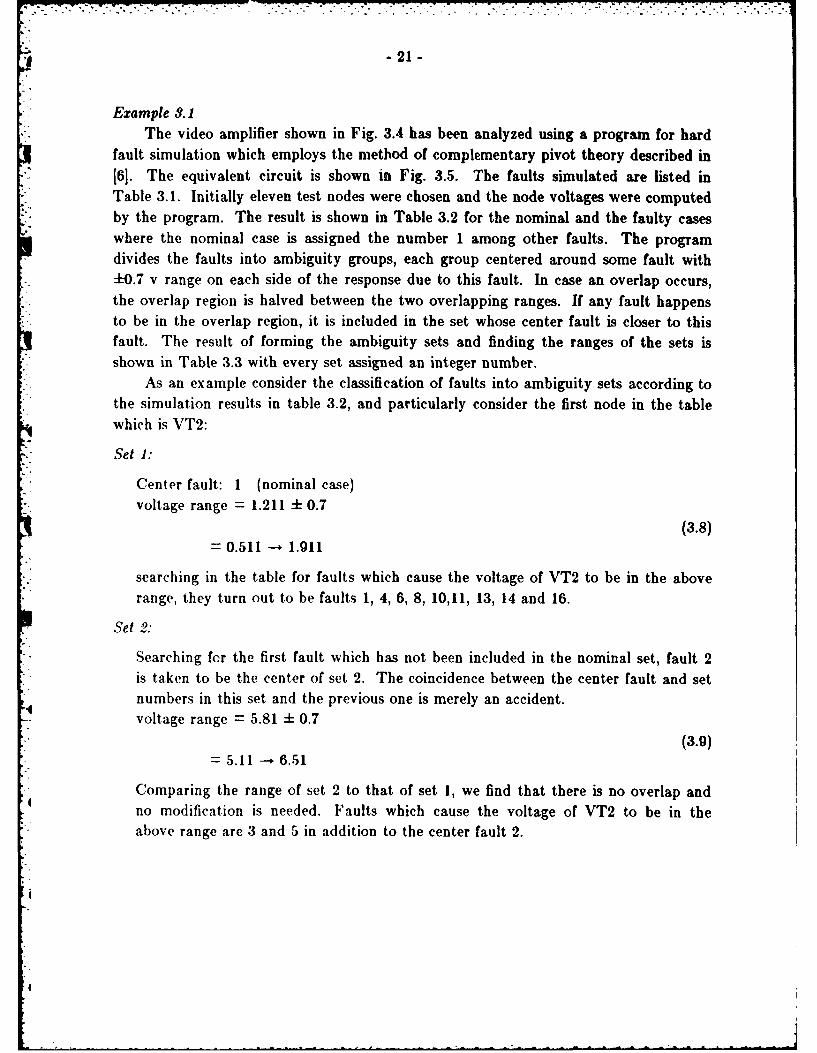
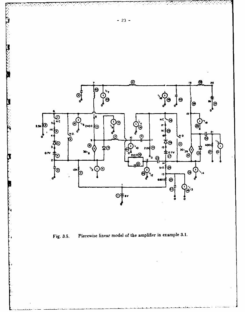
Example 3.1The video amplifier shown in Fig. 3.4 has been analyzed using a program for hard

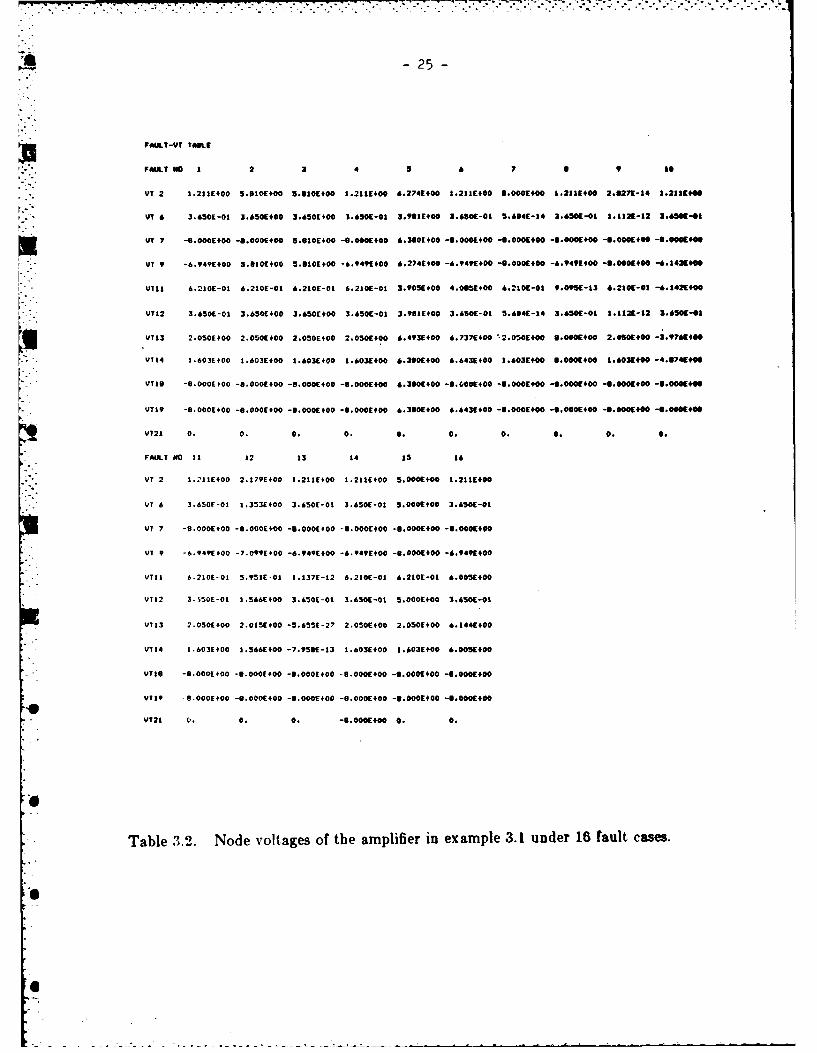
fault simulation which employs the method of complementary pivot theory described in[6]. The equivalent circuit is shown in Fig. 3.5. The faults simulated are listed inTable 3.1. Initially eleven test nodes were chosen and the node voltages were computed

* by the program. The result is shown in Table 3.2 for the nominal and the faulty caseswhere the nominal case is assigned the number 1 among other faults. The programdivides the faults into ambiguity groups, each group centered around some fault with±0.7 v range on each side of the response due to this fault. In case an overlap occurs,

*the overlap region is halved between the two overlapping ranges. If any fault happensto be in the overlap region, it is included in the set whose center fault is closer to thisfault. The result of forming the ambiguity sets and finding the ranges of the sets isshown in Table 3.3 with every set assigned an integer number.

As an example consider the classification of faults into ambiguity sets according tothe simulation results in table 3.2, and particularly consider the first node in the table

* which is VT2:

Set 1:

Center fault: 1 (nominal case)voltage range = 1.211 - 0.7

(3.8)

-0.511 -. 1.911

searching in the table for faults which cause the voltage of VT2 to be in the aboverange, they turn out to be faults 1, 4, 6, 8, 10,11, 13, 14 and 16.

Set 2:

Searching for the first fault which has not been included in the nominal set, fault 2is taken to be the center of set 2. The coincidence between the center fault and setnumbers in this set and the previous one is merely an accident.voltage range = 5.81 ± 0.7

(3.9)= 5.11 -"* 6.51

Comparing the range of set 2 to that of set 1, we find that there is no overlap andno modification is needed. Faults which cause the voltage of VT2 to be in theabove range are 3 and 5 in addition to the center fault 2.

-22-

44C

042u , -0p

5:

232

4 IV

.4.

Fig 3. .

P eIs e i e r m d l o h m lfe

n e a p e 3 1

-24-

Table 3.1. Definition of Faults.

number description

1 nominal case2 L I and/or L2 open3 L4 open4 L3 open5 L7 open

6 L5 and/or L6 open

7 Qibase open8 Q2 base open9 C4 shorted

10 C6 shorted

11I C3 shorted12 C5 shorted13 C8 shorted

14 C9 shorted15 Q1, B-E shorted

16 Q2, B-E shorted

.7

a -25

FILLT-VT TABLE

FALT #O 1 2 3 4 5 6 7 9 to

VT 2 1.2111400 5.60140E0 5.910E+00 1.2111+00 6.274E#00 1.211E+00 9.000E+00 1.2119400 2.921-14 1.2311E144

VT 6 3.650E-01 3.6504+00 3.650(400 3.651-01 3.914+00 3.6501[-01 5.641-14 3.650-01 I.IIA-12 2.65041

VT 7 -. 0OOE00 -6.00(400 5.610E400 -00)01.00 6.360Ot00 -. OO(400 -3.000(00 -304)OO(00 -8.O0+oO -2.00"01.0

VT 9 -6.949E400 5.310(00 5.IO[4.00 -6.949(400 6.274(000 -6.9494+00 -6.000E400 -6.9499#00 -3.000E400 -6.14214*

VII 6.210E-01 6.210E-01 6.2106-01 6.210E-01 3.9051+00 4.065E400 6.2101-01 9.091-13 6.2101-01 -6.1421400

VT12 3.650E-01 3.650E400 3.650'100 3.650E-01 3.911E+00 3.650E-01 5.664E-14 3.6501-01 1.112-12 3.650C-41

VT13 2.050E+00 2.050E400 2.050E#00 2.050E400 6.493(400 6.737E400 "2.05014O0 6.000E00 2.0501400 -3.9761400

VTI4 1.603E400 1.603E400 1.603E400 1.603(400 6.390(400 6.643E1+00 1.603E400 O.0004+00 1.6031400 -438741440

VTII -B.0006400 -6.000(400 -6.0001400 -6.00014#00 6.380E+00 -3.0001400 -9.0001+00 -6.0001400 .4.0001400 -@.00014*

VTi9 -9.000E400 -6.00O400 -3.000E400 -9.000E400 6.390E400 6.643E400 -6.0004+00 -6.0004+00 -8.00014 0 -6.000E400

Re VT21 0. 0. 0. 0. 0. 0. 0. 0. 0. 6.

rULT 00 11 12 13 14 15 16

VT 2 1.'I1I(400 2.1794+00 1.2114+00 1.2111400 5.0004+00 1.2114+00

VT 6 3,650F-01 1.353E400 3.650E-01 3.650E-01 5.000(1400 3.6504-01

VT 7 -8.000(00 -9.0004 00 -. O006+00 -8.000(400 -8.000E400 -3.0001400

VT 9 -6.949E+00 -7.0994+00 -6.949E+00 -6,949E400 -3.00I0(00 -6.949E400

VTII 6.2106-01 5.951E-01 1.137E-12 6.210E-01 6.210E-01 6.OOS'400

VII2 3.$S06-01 1.566E400 3.650E-01 3.6501-06 5.000(400 3.650E-01

VT13 2.050E400 2.0154+00 -5.655E-27 2.050E4+00 2.050E+00 6.1441400

V114 1.603E400 1.5661400 -7.953E-13 1.603E+00 1.603100 6.0051400

VIe -8.006400 -3.0006+00 -.10001400 -8.000(400 -6.0001+00 -6.0001400

VI19 -8.000E400 -6.000(400 -. O00E400 -9.000E+00 -6.000E400 -9.000400

VT2I V. 0. 0. -3.000400 0. 0.

e

• Table 3.2. Node voltages of the amplifier iD example 3.1 under 16 fault cases.

0e

.6 . . . .1d " . L . J j ' " . .. . . . _ ' % -

-~~~~~~~~~ .. &........ . . . . . . . . . . ... .. .. .. .. ....

- 26 -

Set 3.

The center fault of set 3 is the first fault which has not been included in any of thetwo previous sets. This turns out to be fault 7.voltage range = 8.0 - 0.7

(3.10)=7.3- 8

The upper voltage of the range is taken to be 8.0 not 8.7 because the maximumsupply voltage is 8.0 volts. A search in Table 3.2 indicates that fault 7 is the onlyone in this set. The voltage range does not overlap with previous ranges.

Set 4:

Center fault: 9voltage range = 0.0 - 0.7

(3.11)

-0.7 --+ 0.7

By comparison to previous ranges, we find that this range overlaps with the range ofset 1. Henceforth modification is needed to lower the upper voltage of this rangeand raise the lower voltage of the range of set 1. This results involtage range of set 4: -0.7 -- 0.605voltage range of set 1: 0.605 --- 1.911Fault 9 turns out to be the only fault in set 4.

Set 5:

Center fault: 12voltage range = 2.179 - 0.7

(3.12)= 1.479 - 2.879

No overlap exists with any previous range, and the set contains no other fault4 beside fault 12.

*. Set 6:

Center fault: 15voltage range = 5 - 0.7

= 4.3 - 5.7

Modification of the overlapping ranges of this set and of set 2 results in:voltage range of set 6 = 4.3 - 5.345

(3.13)

4 voltage range of set 2 = 5.345 -. 6.51

No other faults exist in set 6.

-4 .. . . ; _

A - 27-

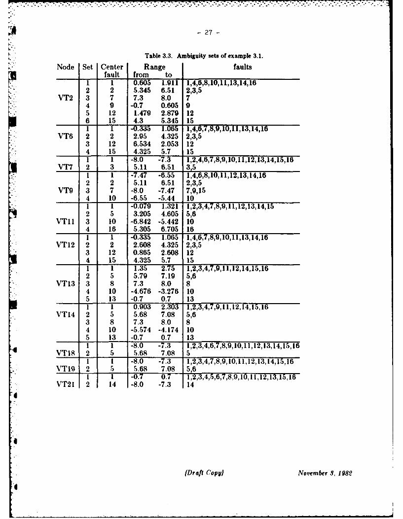
Table 3.3. Ambiguity sets of example 3.1.

Node Set Center Range faultsfault from to

1 1 0.605 1.911 1,4,6,8,10,11,13,14,162 2 5.345 6.51 2,3,5

VT2 3 7 7.3 8.0 74 9 -0.7 0.605 g5 12 1.479 2.879 12

i 6 15 4.3 5.345 151 1 -0.335 1.065 1,4,6,7,8,9,10,11,13,14,16

VT6 2 2 2.95 4.325 2,3,53 12 6.534 2.053 124 15 4.325 5.7 151 1 -8.0 -7.3 1,2,4,6,7,8,9,10,11,12,13,14,15,16

VT7 2 3 5.11 6.51 3,51 1 -7.47 -6.55 1,4,6,8,10,11,12,13,14,162 2 5.11 6.51 2,3,5

VT9 3 7 -8.0 -7.47 7,9,154 10 -6.55 -5.44 101 1 -0.079 1.321 1,2,3,4,7,8,9,11,12,13,14,152 5 3.205 4.605 5,6

VTII 3 10 -6.842 -5.442 104 16 5.305 6.705 161 1 -0.335 1.065 1,4,6,7,8,9,10,11,13,14,16

VT12 2 2 2.608 4.325 2,3,53 12 0.865 2.608 124 15 4.325 5.7 151 1 1.35 2.75 1,2,3,4,7,9,11,12,14,15,162 5 5.79 7.19 5,6

VT13 3 8 7.3 8.0 84 10 -4.676 -3.276 10

__ 5 13 -0.7 0.7 131 1 0.903 2.303 1,2,3,4,7,9,11,12,14,15,16

VTI4 2 5 5.68 7.08 5,63 8 7.3 8.0 84 10 -5.574 -4.174 105 13 -0.7 0.7 131 1 -8.0 -7.3 1,2,3,4,6,7,8,9,10,11,12,13,14,15,16

VT18 2 5 5.68 7.08 51 1 -8.0 -7.3 1,2,3,4,7,8,9,10,11,12,13,14,15,16

VTI9 2 5 5.68 7.08 5,61 1 -0.7 0.7 1,2,3,4,5,6,7,8,9,10,11,12,13,15,16

VT21 2 14 -8.0 -7.3 14

(Draft Copy) Notmmber 8. 1982

I1

- 28-

The intersection process is started by the two nodes having the maximum numbers*of sets which are VT2 (6 sets) and VT13 (5 sets) as shown in Table 3.4. The result of

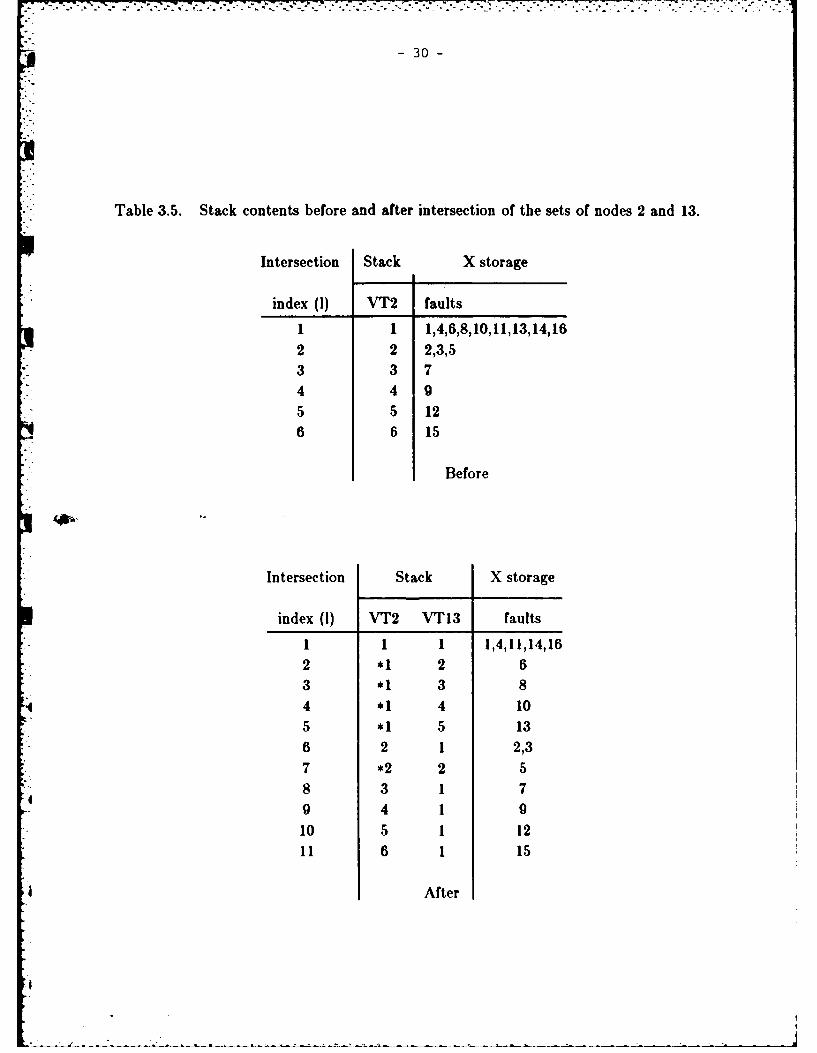
intersection is eleven nonempty sets. The faults in those new sets are listed in thematrix location identified by the row and the column corresponding to the generatingsets of VT2 and VT13 respectively. The fault code at this stage consists of only twodigits denoting the numbers of the intersecting sets of the corresponding nodes. This isshown in Table 3.5 in an array form before and after intersection. The stack contentsbefore intersection consisted only of the indices of the ambiguity sets of VT2 in thecorresponding column. After intersection with the sets of VT13 the stack wasexpanded to accommodate the 11 sets. The stars to the left indicate that the contentsof the stack were pushed down at this position. This happened when an original sethad more than one intersection with the new sets in which case the original code had tobe repeated. The sequence of nodes considered in intersection is VT2, VT13, VTI4,

* VT6, VT9, VT11, VTI2, VT7, VT18, VTI9 and VT21. The stack contents and thefaults in the corresponding ambiguity sets after intersection with every irredundantnode are shown in Table 3.6. The number of sets after intersection with nodes 14, 6, 9,12, 18 and 19 did not increase. Therefore these nodes were excluded from the diction-ary.

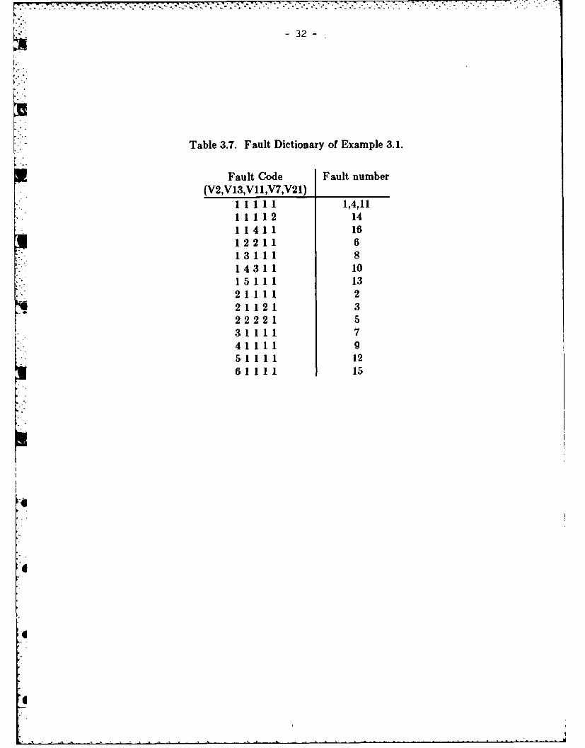
The final table of fault codes (Table 3.7) has two faults (4 and 11) unisolated.Referring to the fault list in Table 3.1, these turn to be L3 open and C3 short. In suchcases the degree of isolation may be accepted and each of the two components may bechecked individually after the test if measuring the five nodes 2, 13, 11, 7 and 21 yieldsthe nominal d.c. response, (Note that faults 4 and 11 are in the nominal ambiguity set)which does not add much more effort. In other cases of more ambiguity, d.c. inputstimuli may have to be used to reduce the ambiguity as will be seen in a later section.

3.4 Fault locationTo illustrate the use of the dictionary, suppose that we have the following meas-

urements obtained from a faulty video amplifier:

VT2=1.2 , V13=8.0, V11=0.5, V7=-8.0 and V21=-8.0

Referring to Table 3.2, we find that the fault is in ambiguity set 1 of node 2, set 3 ofnode 13, set 1 of node 11, set I of node 7 and set I of node 21. The integer code is

then 13111. Now referring to Table 3.7 we find that this corresponds to fault 8.Further referring to Table 3.1 we see that it means transistor Q2 base open.

-29

Table 3.4. Intersection of the ambiguity sets of nodes VT2 and VT13.

_____________VT13

Set ___ 1 2 3 4 51,2,3,4,7,

Faults 9,11,12,14, 5,6 8 10 13

1 10,11,13 16

2 2352,35V'T 3 7 7

5 12 126 15 15

-30-

Table 3.5. Stack contents before and after intersection of the sets of nodes 2 and 13.

Intersection Stack X storage

index (1) VT2 faults

1 1 1,4,6,8,10,11,13,14,162 2 2,3,53 3 74 4 95 5 126 6 15

Before

Intersection Stack X storage

index (1) VT2 VT13 faults

2 *1 2 63 *1 3 8

44 *1 4 105 *1 5 136 2 1 2,37 *2 2 58 3 1 79 4 1 0

10 5 1 1211 6 1 15

After

- 31 -

Table 3.6. Stack contents and isolated faults after intersection with irredundantnodes.

Intersection Stack X storage

index (1) VT2 VT13 VT1I Faults1 1 1 1 1,4,11,142 *1 1 4 163 1 2 2 64 1 3 1 85 1 4 3 106 1 5 1 137 2 1 1 2,38 2 2 2 59 3 1 1 7

10 4 1 1 911 5 1 1 1212 6 1 1 15

a) After intersection with VTII

Intersection Stack X storage

Index (!) VT2 VT13 VTII VT7 Faults1 1 1 1 1 1,4,11,142 1 1 4 1 163 1 2 2 1 64 1 3 1 1 85 1 4 3 1 106 1 5 1 1 137 2 1 1 1 28 *2 1 1 2 39 2 2 2 2 5

10 3 1 1 1 711 4 1 1 1 912 5 1 1 1 1213 6 1 1 1 15

b) After intersection with VT7

0

-32-

Table 3.7. Fault Dictionary of Example 3.1.

Fault Code Fault number(V2,V13,V1 1,V7,V21)

I11 11 1,4,111I1 1112 141 1411 16122 11 6131 11 81431 1 101 51 11 1321 1 11 22 112 1 322 2 21 531 111 741 1 11 951 1 11 1261 1 11 15

ai -33-

4. BINARY REPRESENTATION OF THE ALGORITHM

The better insight into the problem which we will have through its binary aspectwill reflect into easier implementation of the software of the isolation algorithm and the

hardware of the ATE. It will also provide the solution to the problem of minimizing

the number of test nodes. The binary nature of the problem arises from two basic

features:

1. The measured response will either be in a particular range or not.

2. If a response is found to be in a certain range, a fault will either be in the

ambiguity -et identified by this range or not, (i.e. it could be one of the possiblefaults to have caused the trouble or not.)

The first feature has been shown to convert the ambiguity set range

to a binary variable which takes the value one if the response lies within the

range and takes the value zero otherwise as shown in Fig. 3.1.

4.1 Ambiguity Set-Fault Truth TableIn the same sense, every fault can be considered as a binary variable which is a

function of all ambiguity sets of all the n test nodes. Every fault will take the value

one exactly n times when the binary variables representing the corresponding ambi-

guity sets containing the fault are equal to one. Any other combination of binary

values for the ambiguity sets will result in a value zero. In Table 4.1 a truth table is

shown for the m binary functions representing the faults in terms of all the binary vari-

ables representing the ambiguity sets. The number of these binary variables is equal ton

N = Li, where L i is the number of ambiguity sets of node i. The binary variablei=!

representing ambiguity set k of node i is written as v(i,k). The term denoted by this

set means that vb(i,k) takes the value 1 while the other sets assume an unknown combi-

nation. This combination itself is actually immaterial as will be shown in the isolation

process. The total number of possible combinations of the N variables {(v(i,k)} is equal

* to 2 N . However N terms are only shown because the rest (2N-N) terms cannot happen.

They cannot happen because the combination of sets is determined by the faults which

have possibly occurred, and the reduced truth table give all such possi4 ties. The"can' t happen terms" are useful in obtaining minimal realization.

The problem of fault isolation can now be stated in terms of binary function reali-

zation. It is required to synthesize a combinational binary logic whose input is the

binary variables for the ambiguity sets (derived from the measurements as in Fig. 3.1)and whose output consists of m lines representing the m binary functions representing

the m faults. Therefore the fault isolation system can be considered as an ambiguity

O set-fault decoder. As such, the fault location task is accomplished using exactly the

* same binary logic obtained during isolation. However, there are various aspects of the

-

-34-

*Table 4. 1. Truth table of the binary functions representing the m faults.

f1b f2b f3b .. mb

Vb(1, 1) 1 0 0 1

Vb(2,2) 0 1 1 0

Vb(1,L) 0 0 0 0

Vb(2,1) 0 1 0 1

Vb(2,2) 1 0 0 0

Vb(2,L 2) 0 0 1 0

Vb(3, 1) 0 0 1 0

Vb(3,2) 0 0 0 1

Vb(3,L 3) 1 1 0

Vb(n, 1) 0 1 0 1

vb(n, 2 ) 1 0 0 0

Vb(n,Lfl) 0 0 1 0

~- 35 -

ATE hardware implementation, one of which will be considered in a comparison of thestorage requirements against the minimum squared deviation algorithm.

If the realization of the functions {fib} was to be considered separately for everyindividual function, it would have been a straight forward sum of products (SOP) reali-zation [0]. However, there are two problems involved that have to be simultaneously

solved.

1. Finding minimal expressions for all the faults.2. Assuring that there is no more than one fault condition having the same reali-

zation except to the degree of isolation required.

A simple hypothetical example will be first shown to clarify that the sum of pro-

duct realization will tend to be a single product term which is not canonical (i.e. does

not include all ambiguity set variables). However it includes a variable from everynode. The significance of this will be discussed.

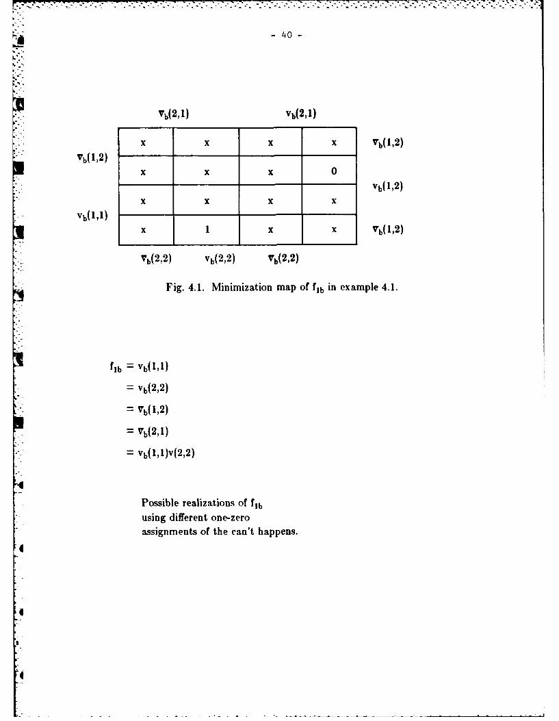
Example 4.1Consider a 3-fault, 2-node case with each node having two ambiguity sets. Table

4.2 shows the reduced and complete truth tables of the problem. The only canonical

SOP term which will make fib = 1 is vb(l,l).b(l, 2 ).Vb( 2 ,1).Vb(2,2) where the dotdenotes logical AND and the bar denotes the complement. Because the ambiguity setsof any one node are mutually exclusive (i.e. only one of them can equal one), the fol-lowing relations hold true:

Vb(1,1).Vb(l, 2 ) - Vb(1,1) (4.1)

Vb(2,1).vb(2,2) = vb(2,2) (4.2)

Hence

fib = vb(1,1)'Vb(1,2) (4.3)

This expression in (4.3) is the same as one of the expressions obtained for f, using theclassical minimization map as shown in Fig. 4.1.

It is clear that the realization which uniquely identifies every fib is in general the

term represented by the product of the ambiguity sets including the fault, which can be0 obtained directly from the complete truth table (table 4.2) without referring to the

map. This can be done if we consider only the prime implicant of fi such thatcorresponding values for other functions are zero or "can't happen". Then use therelation

fl vb(i,k)Vb(i,I- n vb(i,k) (4.4)for all k and I for all k

-

-36-

Table 4.2. Truth table of example 4.1.

Reduced Truth Table of Example 4.1.

f1b f2b f3bVb(1) =1 1 0 0Vb(1,2) =1 0 1 1

Vb(2,) =1 0 1 0

Vb(2,2) = 1 1 0 1

Complete truth table of example 4.1.

0 0 0 0 x x

0 0 1 1 x x0 0 1 1 x x

o 1 0 0 x xo 1 0 1 x x 00 1 1 0 0 10 x x1 0 0 0 x x x1 0 0 1 1 0 x1 0 1 0 x x 11 0 1 1 x x x

411 0 0 x x x11 0 1 x x x

111 0 x x x1 11 x x x

x can't happen

-- - - --

-37-

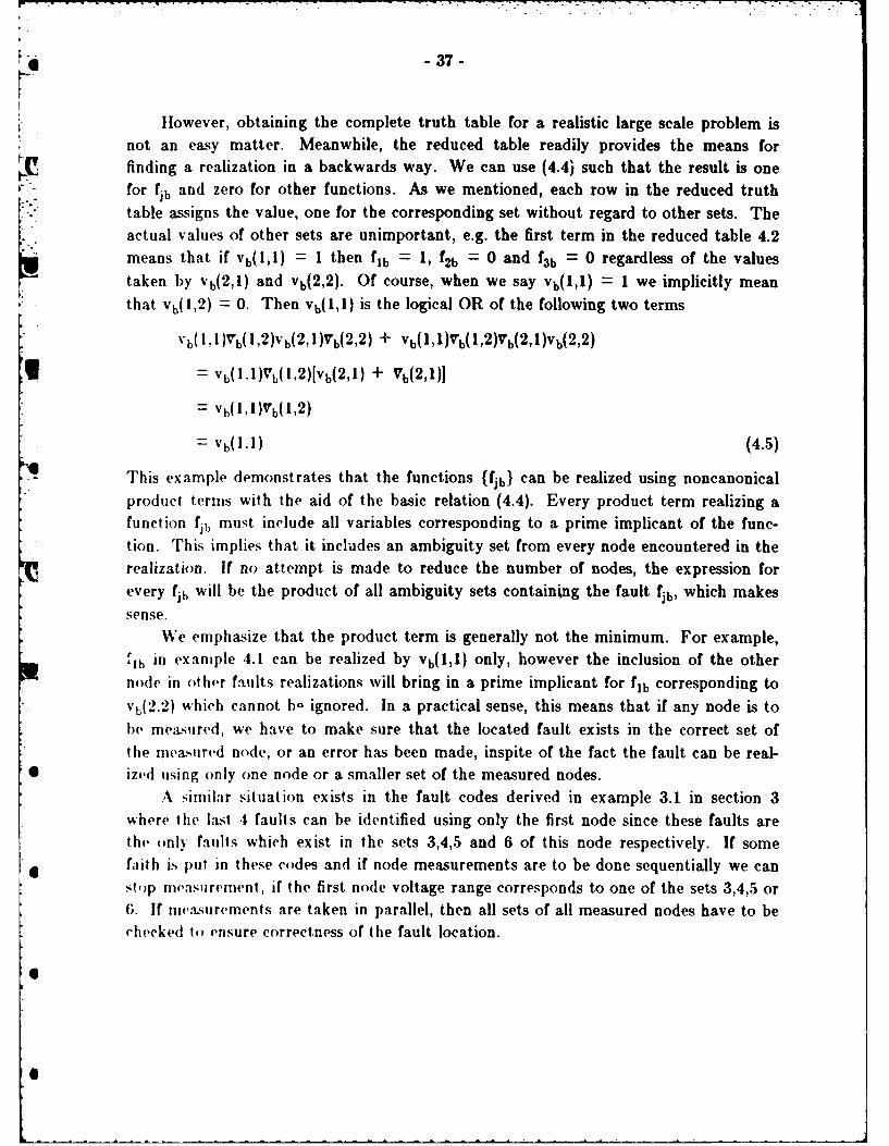
However, obtaining the complete truth table for a realistic large scale problem isnot an easy matter. Meanwhile, the reduced table readily provides the means forfinding a realization in a backwards way. We can use (4.4) such that the result is one

for and zero for other functions. As we mentioned, each row in the reduced truthtable assigns the value, one for the corresponding set without regard to other sets. Theactual values of other sets are unimportant, e.g. the first term in the reduced table 4.2means that if Vb(l,l) = 1 then fib = 1, f2b = 0 and f3b = 0 regardless of the valuestaken by vb(2,1) and vb(2,2). Of course, when we say Vb(1,1) = 1 we implicitly mean

,* that vb(1, 2 ) = 0. Then vb(l,l) is the logical OR of the following two terms

b(l,2)Vb(2,I)rb(2,2 ) + Vb(l,l)Vbl,2)Vb(2,l)Vb(2,2)

*g - Vb(l,l)Vb(l,2)[Vb(2,1) + Vb(2,1)]

- vb(, l)rb(1, 2 )

- Vb(ll) (4.5)

This example demonstrates that the functions {fib} can be realized using noncanonicalproduct terms with the aid of the basic relation (4.4). Every product term realizing afunction fib must include all variables corresponding to a prime implicant of the func-tion. This implies that it includes an ambiguity set from every node encountered in therealization. If no attempt is made to reduce the number of nodes, the expression forevery fib will be the product of all ambiguity sets containng the fault fib, which makessense.

We emphasize that the product term is generally not the minimum. For example,11h in example 4.1 can be realized by vb(1,1) only, however the inclusion of the othernode in other faults realizations will bring in a prime implicant for f1b corresponding to

vb( 2 ,2) which cannot b, ignored. In a practical sense, this means that if any node is tobe mea.sured, we have to make sure that the located fault exists in the correct set ofthe measured node, or an error has been made, inspite of the fact the fault can be real-

* ized using only one node or a smaller set of the measured nodes.A similar situation exists in the fault codes derived in example 3.1 in section 3

where the last 4 faults can be identified using only the first node since these faults arethe only faults which exist in the sets 3,4,5 and 6 of this node respectively. If somefaith is put in these codes and if node measurements are to be done sequentially we canstop measurement, if the first node voltage range corresponds to one of the sets 3,4,5 orG. If nwamsurements are taken in parallel, then all sets of all measured nodes have to bechecked to ensure correctness of the fault location.

6

-38-

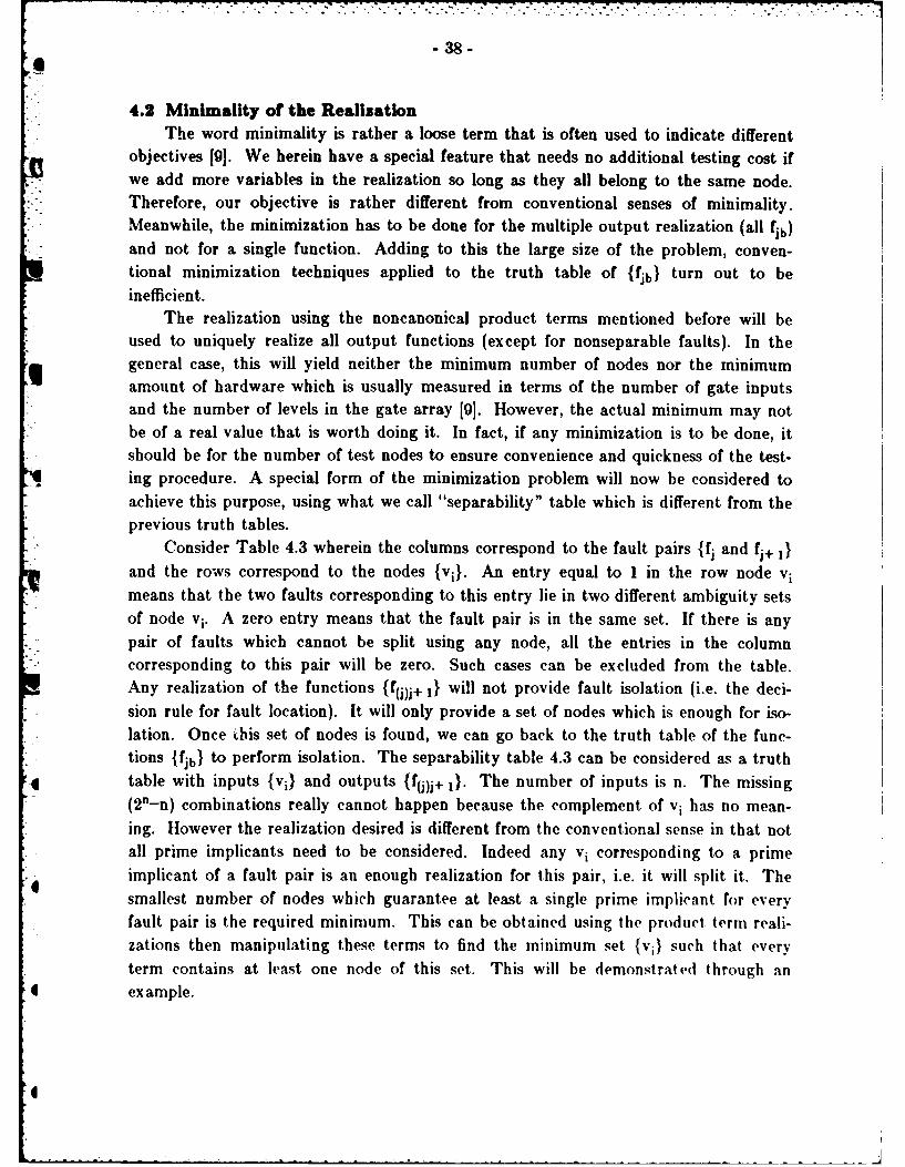
4.2 Minimallty of the RealizationThe word minimality is rather a loose term that is often used to indicate different

objectives [9]. We herein have a special feature that needs no additional testing cost if" we add more variables in the realization so long as they all belong to the same node.

Therefore, our objective is rather different from conventional senses of minimality."- Meanwhile, the minimization has to be done for the multiple output realization (all fib)

and not for a single function. Adding to this the large size of the problem, conven-tional minimization techniques applied to the truth table of {flb) turn out to beinefficient.

The realization using the noncanonical product terms mentioned before will beused to uniquely realize all output functions (except for nonseparable faults). In thegeneral case, this will yield neither the minimum number of nodes nor the minimumamount of hardware which is usually measured in terms of the number of gate inputsand the number of levels in the gate array []. However, the actual minimum may notbe of a real value that is worth doing it. In fact, if any minimization is to be done, itshould be for the number of test nodes to ensure convenience and quickness of the test-ing procedure. A special form of the minimization problem will now be considered toachieve this purpose, using what we call "separability" table which is different from theprevious truth tables.

Consider Table 4.3 wherein the columns correspond to the fault pairs {fj and fj+ 1}and the rows correspond to the nodes {vi). An entry equal to 1 in the row node vimeans that the two faults corresponding to this entry lie in two different ambiguity setsof node vi. A zero entry means that the fault pair is in the same set. If there is anypair of faults which cannot be split using any node, all the entries in the columncorresponding to this pair will be zero. Such cases can be excluded from the table.Any realization of the functions {f(j)j+ 1} will not provide fault isolation (i.e. the deci-sion rule for fault location). It will only provide a set of nodes which is enough for iso-lation. Once iis set of nodes is found, we can go back to the truth table of the func-tions {fib) to perform isolation. The separability table 4.3 can be considered as a truth

*t table with inputs {vi} and outputs (f(j)j+ 1). The number of inputs is n. The missing(2n-n) combinations really cannot happen because the complement of vi has no mean-ing. However the realization desired is different from the conventional sense in that notall prime implicants need to be considered. Indeed any vi corresponding to a primeimplicant of a fault pair is an enough realization for this pair, i.e. it will split it. Thesmallest number of nodes which guarantee at least a single prime implicant for everyfault pair is the required minimum. This can be obtained using the product, term reali-zations then manipulating these terms to find the minimum set {vi) such that everyterm contains at least one node of this set. This will be demonstrated through anexample.

-

* 39

Table 4.3. Separability table.

f 12 f 13 f14 f23 f24 f(j)j + I f(m-1)mv1 1 0 0 0 0 10

V2 1 0 0 0 0 10V3 1 1 1 1 1 0 1

Vn 0 0 0 0 0 1 1

-40-

Vb(2,1) Vb(2,I)

x x x x rb(1,2)Vb(1, 2)

x x x 0Vb(1,2)

x x x xVb(I 1)

X I x x Vb(1,2)

Vb(2,2) Vb(2,2) Vb(2,2)

Fig. 4.1. Minimization map of fib in example 4.1.

fib = Vb(1,1)

= Vb(2,2)

-Vb(1,2)

= Vb(2, 1)

= Vb(1,1)v(2,2)

Possible realizations Of fib

using different one-zeroassignments of the can't happens.

- 41-

Ezample 4.2Consider the separability table 4.4 for a 5-node 5-fault case, each node having 2

ambiguity sets. The fault contents of the sets are shown in Table 4.5. The productterm realizations for the 10 different combinations of fault pairs can be easily deducedfrom the separability table as follows:

f 12 - v 4v5

f 13 - v2 v 3v 4

f 14 = VlV3 V 4 V5

f 15 -VV2V3

f23= VV 3 V5

f2 4 = viv 3

f25= VlV2 V3V4 V5

f3 4 = VIV 2 V5

f35= VV 4

f45 = v2v4v5

The minimum number of nodes required for isolation is the number of nodes whichif retained in the table while other nodes are excluded, a realization can still beobtained in the form of a product term for every fault pair. Some of the terms mayinclude only a single node which is also a realization meaning that the correspondingfault pair cannot be split without this node. Finding the smallest set of nodes whichwill achieve this goal is not easy in the general case. However, the problem can besimplified by absorbing the redundancy in the expression via logical ORing of all the 10expressions. This gives

K = v4v5 + v2 v3 v4 + VIV 3 V4V5 + VIV 2 V3+ V2V3 Vs+ VlV3

+ VI V2 V3V4 Vs+ VIV 2V5 + VI V4 + V2V4V 5 (4.6)

Applying the following basic Boolean algebraic relation to the underlined terms [9]:

X+ XY =X (4.7)

we obtain the following simplification:

K = V4 V5+ V2 V3V4+ VlV 2V3 + V2 v 3 v5 + VlV 3 + V I V2 V5

= vIv 4 + v2 v 4v-5 (4.8)

I

-42-

Table 4.5. Ambiguity sets of example 4.2.

Setnode 12

Vi f 1,f2, f3 f4, f5V 2 f 142,f4 f3A?V3 fI4f2 ff,

V 4 f II 5 ff,V5 f~ N ________

Table 4.4. Separability table of example 4.2.

f 12 f13 f14 fIS f23 f24 f2,5 f34 f3-5V1 0 0 1 1 0 1 1 1 1V2 0 1 0 1 1 0 1 1 0V3 0 1 1 1 1 1 1 0 0

4V 4 1 1 1 0 0 0 1 0 1VS 1 0 1 0 1 0 1 1 0

4

*-43-

K - v 4 v 5 + VIV 3 + V2V3 V4 + v 2v 3 vS+ VIV2Vs+ VlV4

In a brute force manner we can tell that there are five possible solutions each provides3 nodes if only retained in the expression of (4.8) each term will still have at least onevariable (node). The solutions are (v1,v2,v4), (v1,v3 ,v4), (v1,v2 ,v), (VI,V3 ,V5 ) and(V3 ,V4 ,V5 )"

It is interesting to see that this problem has a graph theoretic equivalent known asthe minimum feedback edge set problem [10]. The complexity of the computer imple-mentation of the minimization algorithm is exponential in the number of variables [8].

4.3 Fault IsolationHaving obtained the minimum set of nodes, we can go back to the original truth

table to find the SOP realization which will be a single product term including anambiguity set from every node (after excluding redundant nodes). This realizations areguaranteed to identify every fault uniquely, i.e. there should be no more than one faulthaving the same expression except any pair of faults which may have been excludedbefore minimization.

There is an obvious effort in the process of minimization represented in formingthe separability table then finding the minimum especially because the dimensionalityof the separability table is larger than that of the original truth table. The number of

fault pairs in m faults is r(m-l) which is larger than m if m is greater than 3. If2

ensuring a minimal number of nodes is not a concern we can find the product termrealizations directly from the original truth table and try simultaneously to solve thesecond problem mentioned in the beginning of this section. This means that we have

to make sure that any realization we obtain for any of the faults is not a valid realiza-tion for any other fault. This can be done only if we operate on all faults simultane-ously. For example if fj is to be realized by v(il,kl)v(i 2 ,k2)v(i 3 ,k3), then fj is equal to

one if all these three sets are also equal to one. Then every other fault must be equal tozero when these sets are all equal to one, i.e. the product (logical ANDing) of the

0entries corresponding to these sets under every other fault must be zero. This meansthat to realize fi and in the same time avoid valid realizations for other faults we willbe taking the logical AND of the corresponding entries in the whole rows characterizingthe ambiguity sets being considered which is nothing but taking the intersection of the

* sets, which has been used before. There are two ways for the intersection process to* proceed:

I. Considering every fault fib separately and performing the intersection until weget, a single nonzero element in the row. This element should of coursecorrespond to fib. Then the process is repeated for all faults. The test nodes

required in this case are the collection of all nodes realizing all faults.

." - .-- - " - " - . . . . . . . "".... . . . . . - * .. 'h.:w' " ' r- .,' _ '- . ', ' -. :- .-

- 44-

2. Following the same objective set in section 3, i.e. intersecting the ambiguity setsin pairs and storing the result of intersection aiming at obtaining m rows each ofthem having a single nonzero element. This is exactly the same method followedin section 3 except that the intersection can now be obtained using logical AND-ing of rows which may be stored in a single byte of storage.

We prefer the second way since it allows for wise selection of the sequence of setsto be intersected in order to approach the minimum by giving priority to the nodes

having the maximum number of ambiguity sets, which we have also done before.To complete the analogy between the binary and the multivalued forms we will

list the dictionary in the form of binary expressions which can be realized by combina-tional logic.

4.4 Fault LocationAs we mentioned before, the fault location is done directly using the binary expres-

*~ sions derived during the isolation process. The only thing needed in addition to that isto derive the binary input from voltage measurements.

*Complexity of the algorithm: The intersection operation can now be done with greatsimplicity as the fault variables {fkb) will be stored as ones and zeros in one register(computer word) assuming that its length is greater than Nf. Simple logical ANDing of

binary words will replace the intersection of ambiguity sets. The value of thissimplification will be appreciated when the problem size gets larger.

A bound for the execution time can be easily derived in terms of a basic time unitT that takes the following two operations to be done.

i) Parallel ANDing of Nr pairs of bits, or simply ANDing of two computer words.ii) Checking for null intersection, i.e., if the result of ANDing is zero or not. Refer-

ring to Fig. 3.2, we can deduce the following.i) The time t of operations on two groups of sets whose numbers are LI and L2 is

LIxL 2 x T.ii) At any intersection stage, the input number of sets in any of the two groups is less

than Nt. Hence

t < Max(Li) x Nfx T (4.9)

where Max(Li) is the maximum number of sets in all nodes. iii) The number of

intersection stages is at most (N, - 1). Then the overall execution time is boundedaccording to the inequality

toweral < Max(Li) x Nf x (N, - 1) x T (4.10)

Added to this is, of course, the time needed in other manipulations like

>_

,A -45-

incrementing indices, etc.

Firmware: There are various possible ways of building an ATE for trouble shootingIbased on the logical isolation algorithm. One way is by using a digital comparator to

compare the code generated from the test measurements against other codes in the dic-tionary. Another way is by converting the codes to their equivalent binary expressionsand evaluating these expressions using a programmable gate array, for instance, withinputs derived from the ambiguity ranges of the test measurements. For example, thethird entry in the dictionary (12211) corresponding to fault 6 has the binary equivalent.

Kf6b : Vb(l,l)Vb(2,2)vb(3,2)Vb(4,I)Vb(5,l)

If the RIIS expression evaluates to one, fault 6 will be actual fault. Similar expressionshold for the rest of the faults. As such, the ATE can be viewed as an ambiguity set-fault decoder. The binary inputs vb(ij) are derived from measurement of vi accordingto relation 8. An interesting feature is that the input to the ATE does not needA/Dconversion but could be derived from the measured voltages using analog compara-tors as shown in Fig. 3.1.

At any case, the voltage ranges have to be stored in the ATE together with thefault codes. It is interesting to compare the storage requirements of this algorithmagainst those of the least squares method. The latter needs the storage of the fault-node voltage table which requires a storage of capacity S, given by

S, = NN r real numbers

= 2NvN f integers

* The logical isolation requires the storage of the two tables of voltage ranges and faultcodes which requires a capacity S2 bounded by the inequality

S2 N< NV x 2 x Max(L1 ) real numbers

+ [NV x N r] integers

N [N,r + 4 Max(Li) integers

S2 grows as the number of faults while Sn grows as twice this value.

I

ai

U

- 46-

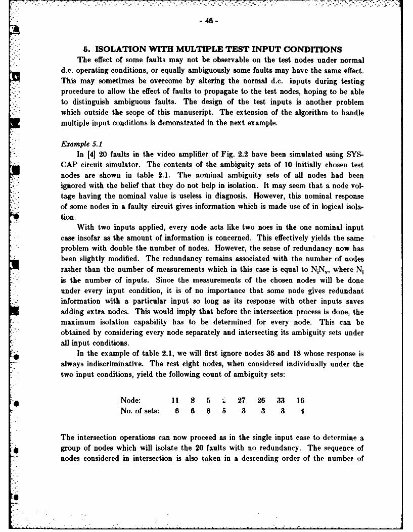
5. ISOLATION WITH MULTIPLE TEST INPUT CONDITIONSThe effect of some faults may not be observable on the test nodes under normal

d.c. operating conditions, or equally ambiguously some faults may have the same effect.This may sometimes be overcome by altering the normal d.c. inputs during testingprocedure to allow the effect of faults to propagate to the test nodes, hoping to be able

*. to distinguish ambiguous faults. The design of the test inputs is another problem.. which outside the scope of this manuscript. The extension of the algorithm to handle

multiple input conditions is demonstrated in the next example.

Example 5.1In [4] 20 faults in the video amplifier of Fig. 2.2 have been simulated using SYS-

CAP circuit simulator. The contents of the ambiguity sets of 10 initially chosen testnodes are shown in table 2.1. The nominal ambiguity sets of all nodes had beenignored with the belief that they do not help in isolation. It may seem that a node vol-tage having the nominal value is useless in diagnosis. However, this nominal responseof some nodes in a faulty circuit gives information which is made use of in logical isola-tion.

With two inputs applied, every node acts like two noes in the one nominal inputcase insofar as the amount of information is concerned. This effectively yields the sameproblem with double the number of nodes. However, the sense of redundancy now hasbeen slightly modified. The redundancy remains associated with the number of nodesrather than the number of measurements which in this case is equal to NiN, where Ni

is the number of inputs. Since the measurements of the chosen nodes will be doneunder every input condition, it is of no importance that some node gives redundantinformation with a particular input so long as its response with other inputs savesadding extra nodes. This would imply that before the intersection process is done, themaximum isolation capability has to be determined for every node. This can beobtained by considering every node separately and intersecting its ambiguity sets underall input conditions.

In the example of table 2.1, we will first ignore nodes 36 and 18 whose response isalways indiscriminative. The rest eight nodes, when considered individually under the

* "two input conditions, yield the following count of ambiguity sets:

Node: 11 8 5 . 27 26 33 16No. of sets: 6 6 6 5 3 3 3 4

The intersection operations can now proceed as in the single input case to determine a-* group of nodes which will isolate the 20 faults with no redundancy. The sequence of

nodes considered in intersection is also taken in a descending order of the number of

* -47-

sets, as it is intuitive that a node having a larger number of sets will have better isola-tion capability. The process is started by nodes 11 and 8 yielding 11 new sets. Theresult of intersecting the rest of the nodes is as follows:

Nodes No. of sets

11,8 1111,8,5 1511,8,5,2 1711,8,5,2,16 1911,8,5,2,16,27 1911,8,5,2,16,27,26 1911,8,5,2,16,27,26,33 19

It is clear that nodes 27, 26 and 33 do not improve the isolation, stopping at only 19sets which means that there is a pair of faults which have not been isolated among theoriginal 20 faults.

There are two possible ways the fault dictionary can be formed and stored in the

ATE.

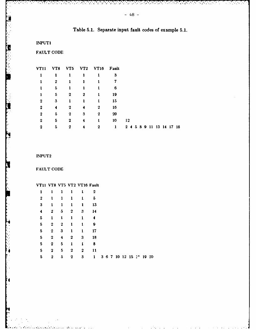
1. If the two input case is viewed as two separate single input cases, then a fault dic-tionary may be generated for each case on the basis that the two inputs need notnecessarily be both applied during the test. The fault codes for the two cases are

shown in Table 5.1. The test should be first performed with the first input applied.-* If there is any ambiguity it will be then resolved by applying the second input. It is

clear of course that faults which are ambiguous with the first input are isolated with-" . the second one with the exception of the pair 10 and 12. The reverse is also true.

As an example, suppose that the fault code is 25242 with the first input applied.The fault is then one of the group (1, 2, 6, 5, 8, 9, 11, 13, 14, 17 and 18). If thesecond input is applied and the code becomes 21111, the actual fault must be fault2. Obviously if the second input was only applied, fault 2 would have been directlylocated. The input to be applied first is naturally the one that isolates more faults,which is input 2 in this case.

2. If the two input conditions are to be both applied before fault location is attempted,the two dictionaries have to be combined. The combined fault codes which isolate18 faults are shown in table 5.2 where the indices of v0 indicate the node and the

input respectively. This of course increases both the storage requirements and theeffort needed in fault location especially if it is done visually. This difficulty in han-dling the test manually when the dictionary size gets bigger may require fullyautomated trouble shooting aids based on the binary representation. At any case,

-48-

Table 5.1. Separate input fault codes of example 5.1.

INPUTI

* FAULT CODE

VTII VT8 VTS5 VT2 MT6 Fault

1 1 1 1 3

1 2 1 1 17

1 5 2 2 1 1

2 3 1 1 1 1

2 4 2 4 2 16

2 5 2 3 2 20

2 5 2 4 1 10 12

2 5 2 4 2 1 2 45 8 911 131417 18

INPUT2

FAULT CODE

* VT11 VT8 VT5 VT2 VT16 Fault

1 1 1 1 2

2 1 1 1 1 5

3 1 1 1 1 13

4 2 5 2 3 14

5 1 1 1 1 4

5 2 2 1 1 9

5 2 3 1 1 17

5 2 4 2 3 18

5 2 5 1 1 8

45 2 5 2 2 11

5 2 5 2 3 1 3 67 10 12 15 ~19 20

S- 49-L" -

COMBINED INPUTS

V11,1 V1I,2 V8,1 V8,2 V5,1 V5,2 V2,1 V2,2 V16,1 V16,2 Fault1 5 1 2 1 5 1 2 1 3 31 5 2 2 1 5 1 2 1 3 71 5 5 2 1 5 1 2 1 3 61 5 5 2 2 5 2 2 1 3 192 1 5 1 2 1 4 1 2 1 22 2 5 1 2 1 4 1 2 1 52 3 5 1 2 1 4 1 2 1 132 4 5 2 2 5 4 2 2 3 142 5 3 2 1 5 1 2 1 3 152 5 4 2 2 5 4 2 2 3 162 5 5 1 2 1 4 1 2 1 42 5 5 2 2 2 4 1 2 1 92 5 5 2 2 3 4 1 2 1 172 5 5 2 2 4 4 2 2 3 182 5 5 2 2 5 3 2 2 3 202 5 5 2 2 5 4 1 2 1 82 5 5 2 2 5 4 2 1 3 10 122 5 5 2 2 5 4 2 2 2 112 5 5 2 2 5 4 2 2 3 1

a

Si

6:i -

- 50-

however, the voltage ranges of the ambiguity sets have to be stored for all inputconditions in order to determine the set indices.

6. CONCLUSIONS AND SUGGESTIONS FOR FUTURE RESEARCHThe method for generating an analog fault dictionary described in this report pro-

vides an efficient tool for fault diagnosis by logical means. The fault isolation algo-rithm presented in section 3 can be easily implemented with some extra software addedto the circuit simulator. The execution time of the fault isolation routine, was shownto be bounded according to the analysis in section 4. Compared to the time needed forfault simulation, the logical fault isolation algorithm needs a trivial length of time. Allthis analysis is done once for all in the pretest stage. The outcome of logical fault isola-tion should be as follows:

1. A set of nodes whose d.c. voltage is to be measured during the test, and should besufficient to achieve the required level of ambiguity in locating the actual fault afterthe test is done. This set of nodes is minimal in the sense that the prescribeddegree of isolation cannot be obtained if any of these nodes is dispensed away with,which implies that none of the nodes is redundant. The term degree of isolationcould roughly mean the number of faults within which the actual fault is ambigu-ous.

2. A table of voltage ranges for every node in the resulting test nodes, where everyrange is given an integer number that identifies an ambiguity group of faults any ofwhich will cause the node voltage to be in the corresponding range. This meansthat the node voltage is effectively quantized into discrete ranges or multivalued log-ical levels. This quantization is expected to be always possible so long as the topol-ogy of the unit under test is such that the simulated faults are clustered in a waythat all faults in a cluster have almost the same effect on a single test measurement.Of course, these clusters are different for different nodes.

3. A table of fault codes where every code identifies a fault or a group of faults up tothe acceptable degree of isolation. Every code consists of integer numbers derived

.4 from those numbers assigned to the voltage ranges. The code length (number ofintegers in the code) is equal to the number of test nodes.

These two tables mentioned above constitute the required fault dictionary whichhas to be stored in the ATE. It has been shown in Section 4 that the storage require-

ments of the logically based analog fault dictionary are less than those of the leastsquare based dictionary. The accompanying hardware is also much easier to imple-ment. For large scale circuits, these advantages are very well appreciable.

The dictionary approach in general, like all other fault diagnosis approaches, can-4 not be claimed to be free from uncertainty which is introduced by statistical variations

in component values and consequently of the circuit response. The efficacy of the

..

dictionary also depends on how exhaustive the fault list is. Even with these drawbacksa dictionary for hard faults can be very efficient in diagnosing a large percentage offaults. The best reliability is achieved when the dictionary is used in conjunction withsoft fault diagnosis routines, like multifrequency diagnosis, whenever it can be afforded.This is not always possible of course. For example, in field repairs where computingfacilities are not available, a fault dictionary would be indispensable.

It may be sometimes possible to locate the fault with only fewer measurementsamong all measurements to be fed to the ATE. In such cases, completing the diction-ary measurements may or may not be necessary depending on the level of confidenceput in the dictionary. However, completing the measurements is preferable to makesure that the located fault does produce the coded response as stored in the ATE. If

Uthe test measurements are all done before attempting to locate the fault, this point willnot be of importance. It is only meaningful if the test measurements are taken sequen-tially. In some other cases, if the code derived from measurements does not match withany other code in the dictionary a strange fault will be acknowledged. This is advanta-

*geous compared to other methods which will simply take the nearest fault on a leastsquares basis and declare it to be the actual fault.

For multiple test inputs, there are two options in compiling and using the faultdictionary.

1. It can be regarded as several single input cases. Then a fault dictionary may begenerated for each test input on the basis that all inputs need not necessarily beapplied during the test.

2. If all inputs are to be all applied before fault location is attempted, the dictionarieshave to be combined as has been shown in section 5. This will generally producelonger fault codes and more storage will be needed. The first approach is recom-mended.

It is believed that the following points are important to be investigated to improve* the performance of a logical fault dictionary:

1. A complete hardware implementation of an ATE based on logical isolation of faults.Several points related to this have been already discussed, e.g. storage requirements,

* interfacing, etc.. For flexibility and possible modifications in the dictionary, amicroprocessor based ATE would naturally be most appropriate.

2. Investigating the effect of the components' statistical variation on the circuitresponse and consequently on the dictionary.

• -, ,. .. ,_, .,.. . ._. - -_ .,-..,- . _ .- . . . ....- . . .- -. -. . . . . . . -' i..--- ',. .. - -. -"

- 52-

3. The design of test inputs for a better degree of isolation. The piecewise linearmodel and the formulation of the circuit equations into a complementary problemform readily provide the ground for this.

p" .

-53-

References

1. R. Duhamel and J. Rault, "Automatic Test Generation Techniques for Analog-.-. Circuits and Systems," IEEE Trans. on Circuits and Systems, Vol. CAS-26, pp.

411-440, July 1979.

2. W. A. Plice, "Overview of Current Automated Analog Test Design," Proc. of the1979 IEEE Test Conference, Cherry Hill, New Jersey, pp. 128-136, September

• .- 1979.

3. R. Saeks, S. P. Singh and R. Liu, "Fault Isolation via Component Simulation,"IEEE Trans. on Circuit Theory, Vol. CT-19, pp. 634-640, Nov. 1972.

4. W. Hochwald and J. Bastian, "A DC Approach for Analog Fault DictionaryDetermination," IEEE Trans. on Circuits and Systems, Vol. CAS-26, pp. 523-529,

- July 1979.

5. A. T. Johnson, Jr., "Efficient Fault Analysis in Linear Analog Circuits," IEEETrans. on Circuits and Systems, Vol. CAS-26, pp. 475-484, July 1979.

6. P. M. Lin, "DC Fault Diagnosis Using Complementary Pivot Theory," Proc. 1982IEEE Int'l. Symp. on Circuits and Systems, pp. 1132-1135, May 1982.

- 7. C. Timaztepe and N. Prywes, "Generation of Software for Computet ControlledTest Equipment for Testing Analog Circuits," IEEE Trans. on Circuits and Sys-tem, Vol. CAS-26, pp. 537-548, July 1979.

8. Narsingh Deo, "Graph Theory with Applications to Engineering and ComputerScience," Prentice-Hall, 1974.

9. E. McCluskey, "Introduction to the theory of switching circuits," McGraw Hill,1965.

. 10. LEMPEL, A., "Minimum Feedback Arc and Vertex Sets of a Directed Graph,"IEEE Trans. on Circuit Theory, Vol. CT-13, pp. 399-403, Dec. 1966.

4.'

,

6i

8I3