arX

iv:h

ep-t

h/03

0618

5v2

16

Jul 2

003

CERN-TH/2003–136

SPIN-03/19

ITP-03/31

hep-th/0306185

New D = 4 gauged supergravities from

N = 4 orientifolds with fluxes

Carlo Angelantonj1,†, Sergio Ferrara1,2,‡ and Mario Trigiante3,

1 CERN, Theory Division, CH 1211 Geneva 23, Switzerland

2 INFN, Laboratori Nazionali di Frascati, Italy

3 Spinoza Institute, Leuvenlaan 4 NL-3508, Utrecht, The Netherlands

e-mail: ⋆ carlo.angelantonj@cern.ch , ∗ sergio.ferrara@cern.ch, M.Trigiante@phys.uu.nl

Abstract

We consider classes of T6–orientifolds, where the orientifold projection contains

an inversion I9−p on 9 − p coordinates, transverse to a Dp–brane. In absence of

fluxes, the massless sector of these models corresponds to diverse forms of N = 4

supergravity, with six bulk vector multiplets coupled to N = 4 Yang–Mills theory

on the branes. They all differ in the choice of the duality symmetry corresponding

to different embeddings of SU(1, 1)×SO(6, 6+n) in Sp(24+2n,R), the latter being

the full group of duality rotations. Hence, these Lagrangians are not related by local

field redefinitions. When fluxes are turned on one can construct new gaugings of

N = 4 supergravity, where the twelve bulk vectors gauge some nilpotent algebra

which, in turn, depends on the choice of fluxes.

1. Introduction

New string or M–theory models are obtained turning on n–form fluxes, which allow,

in general, the lifting of vacua, supersymmetry breaking and moduli stabilisation [1]–[24].

Examples of such new solutions are IIB and IIA orientifolds [25, 26, 27, 28, 29], where the

orientifold projection (in absence of fluxes) preserves N = 4 or N = 2 supersymmetries.

Recently, the T6/Z2 orientifold with N = 4 supersymmetry [8, 9] and K3 × T2/Z2

orientifold [24] with N = 2 supersymmetry have been the subject of an extensive study.

In these cases, turning on NS–NS and R–R three–form fluxes allows to obtain new string

vacua with vanishing vacuum energy, reduced supersymmetry and moduli stabilisation

[7, 8, 9, 21, 24]. These features can all be understood in terms of an effective gauged su-

pergravity, where certain axion symmetries are gauged [31, 30, 32]. These are generalised

no–scale models [33, 34].

In the present investigation, we consider more general four–dimensional orientifolds

with fluxes (both in type IIB and IIA) where the orientifold projection involves an inver-

sion I9−p on 9−p coordinates, transverse to the Dp–brane world–volume, thus generalising

the T6/Z2 orientifold (with p = 3) constructed by Frey–Polchinski [8] and Kachru–Shulz–

Trivedi [9] (see also [10] for a derivation of the complete low–energy supergravity from

T–dialysed Type I theory in ten dimensions). Interestingly, their low–energy descriptions

are all given in terms of N = 4 supergravity with six vector supermultiplets from the

closed–string sector, coupled to an N = 4 Yang–Mills theory living on the Dp–brane

world–volume.

However, despite the uniqueness of N = 4 supersymmetry, the low–energy actions

crucially differ in the choice of the manifest “duality symmetries” of the Lagrangian, since

different sets of fields survive the orientifold projection, and therefore different symme-

tries are manifestly preserved. Leaving the brane degrees of freedom aside, these duality

symmetries are specified by their action on the (twelve) bulk vectors. Actually, N = 4 su-

pergravity demands that such symmetries be contained in SU(1, 1)×SO(6, 6) [35, 36] and

act on the vector field strengths and their duals as symplectic Sp(24,R) transformations

[37]. On the other hand, the symmetries of the Lagrangian correspond to block–lower–

triangular symplectic matrices, whose block–diagonal components have a definite action

on the vector potentials [38, 39, 40]. For instance, in the orientifold models containing an

I9−p inversion, the block–diagonal symmetries always include GL(9−p,R)×GL(p−3,R),

as maximal symmetry of the GL(6,R) associated to the moduli space of the six–torus met-

rics. The lower–triangular block contains the axion symmetries of the R–R scalars and of

the NS–NS ones originating from the B–field, whenever present1.

1For example, the latter is not present in the p = 3 case, i.e. the T6/Z2 orientifold.

1

In the sequel, we describe all nilpotent algebras Np [41], corresponding to axion sym-

metries of the R–R and NS–NS scalars for all orientifold models. All Np’s are nilpotent

subalgebras of so(6, 6), are generically non–abelian and contain central charges. There

are four of them in type IIB (p = 3, 5, 7, 9) with dimensions 15, 23, 23, 15 respectively,

while there are only three of them in type IIA (p = 4, 6, 8) of dimensions 20, 24, 20,

respectively. A common feature of these algebras is that they always contain fifteen R–R

axionic symmetries, while the extra symmetries correspond to NS–NS B–field axions in

the bi–fundamental of GL(9− p,R)×GL(p− 3,R).

A further R–R axion symmetry originates from the SU(1, 1), which acts as electric–

magnetic duality on the gauge fields living on the brane world–volume. The corresponding

axion field can be identified with the Cp−3 R–R field, as dictated by the coupling

∫

Σp+1

Cp−3 ∧ F ∧ F , (1)

where F is the two–form field strength of gauge fields living on the branes.

Turning on fluxes in the orientifold models (three- and five–form fluxes in type IIB,

two- and four–form fluxes in IIA) corresponds to a “gauging” in the corresponding su-

pergravity Lagrangian, whose couplings are dictated by the particular choice of fluxes.

Non–abelian gaugings may also occur corresponding to subalgebras of Np, or quotient

algebras Np/Z, where Z are some of the central generators of Np.

As an illustrative example, let us consider the p = 7 type IIB orientifold defined in sec-

tion 2, where the non–vanishing NS–NS and R–R fluxes are Haij , Faij , Gi = ǫab ǫijkl Gabjkl

(a, b = 5, 6 and i, j = 1, . . . , 4), and let us look at terms involving the axions coming from

the B and four–form fields, Bia and Cijab = Cijǫab. Inspection of the three–form kinetic

term reveals a non–abelian gauge coupling proportional to

√−g Haij Hµνb gab giµ gjν , (2)

as well as axion gauge couplings proportional to

√−g Haij Hµbℓ gab giµ gjℓ , (3)

together with similar expressions for the F–three form. Such terms come also from the

reduction of type IIB four–form field. In addition, when a five–form flux Gi is turned on

an axion gauge coupling emerges of the type

∂µCij + ǫijkℓGk Gℓ

µ . (4)

where Gℓµ = gℓi giµ are the Kaluza–Klein vectors. We report here only a preliminary

analysis of the deformation of the N = 4 supergravity due to these new gaugings.

2

In the present paper we do not address either the question of unbroken supersymme-

tries or the question of moduli stabilisation, which would require the knowledge of the

scalar potential and a study of the fermionic sector. However, we can anticipate that cer-

tain moduli are indeed stabilised in all these models, since a Higgs effect is taking place

as suggested by the presence of charged axion couplings.

The paper is organised as follows: in section 2, we review the four-dimensional T6/Z2

orientifold models, their spectra and their allowed fluxes. In section 3, the N = 4

supergravity interpretation is given for the ungauged case (absence of fluxes) and the

duality symmetries exposed. The Np algebras are exhibited as well as their action on the

vector fields. In section 4, we give a preliminary description of gauged supergravity, for

the particular case of type IIB orientifolds with some three–form fluxes turned on. In

section 5 some conclusions are drawn. Finally, in appendix some useful formulae needed

to compute the quadratic part of the vector field strengths in the Lagrangian, are given.

2. N = 4 orientifolds: spectra and fluxes

In this section we review the construction of orientifold models preserving N = 4

supersymmetries in D = 4 [29]. This is the simplest setting for orientifold constructions,

and consists of modding out type II superstrings by the world–sheet parity Ω [25]. Follow-

ing [28, 29], the orientifold projection can be given a suggestive geometrical interpretation

in terms of non–dynamical defects, the orientifold O–planes, that reflect the left–handed

and right–handed modes of the closed string. Actually, one can combine world–sheet

parity with other (geometrical) operations. In general, this can affect the nature of the

orientifold planes, that, in the simplest instance of a bare Ω have negative tension and

R–R charge, and are (9 + 1)–dimensional (O9 planes) since they have to respect the full

Lorentz symmetry preserved by Ω. In the present paper, we are interested in the class

of models generated by the ΩI9−p generator, where I9−p denotes the inversion on 9 − p

coordinates. Of course, ΩI9−p must be a symmetry of the parent theory, and this is the

case of type IIB for p odd, and of type IIA for p even. Actually, ΩI9−p reflects the action

of T-duality in orientifold models. Indeed, T-duality itself can be thought of as a chiral

parity transformation

XL → XL , XR → −XR , (5)

and conjugates Ω so to get

T9−pΩT−19−p = ΩI9−p . (6)

As a result, the full ten–dimensional Lorentz symmetry is now broken to the subgroup

SO(1, p)×SO(9−p), and the closed–string sector involves O9−p planes sitting at the fixed

points of the orbifold T9−p/I9−p. The associated open-string sector will then correspond

3

to open strings with Dirichlet boundary conditions along T9−p, i.e. open strings ending on

D(9− p) branes. As usual, tadpole conditions will fix the rank of the Chan–Paton gauge

group, i.e. the total number of D-branes. In the present paper, however, we shall not

be concerned with open–string degrees of freedom and we shall concentrate our analysis

solely on the closed-string degrees of freedom.

Before we turn to the description of specific models, a general comment is in order.

An important requirement in the construction is that the orientifold group be Z2, i.e. its

generator ΩI9−p must square to the identity. Although Ω has always ±1 eigenvalues, and

thus Ω2 = 1, this is not the case for I9−p. For example, for p = 7 I2 would correspond to

a π rotation on a two–plane and, although its action on the bosonic degrees of freedom is

real and assigns to them a plus or minus sign according to the number of indices along the

two–plane, its eigenvalue on spinors is eiπΣ , where Σ = ±12are the two helicities. Thus,

it does not square to the identity, but rather to (−1)F , with F the (total) space–time

fermion number. Therefore, in this case the orientifold projection needs be modified by

the inclusion of (−1)FL, with FL the left-handed space–time fermion number [47]. We are

thus dealing with the four-dimensional orientifolds

(Tp−3 × T9−p) /ΩI9−p

[(−1)FL

][ 9−p2 ]

, (7)

where[9−p2

]denotes the integer part of (9−p)/2. Here we have decomposed the six-torus

as

T6 = Tp−3 × T9−p , (8)

since I9−p only acts on the coordinates of T9−p, while leaves invariant those along Tp−3.

As we shall see, this is a natural decomposition since, in the orientifold, we are left with

the perturbative symmetry GL(p − 3) × GL(9 − p) of the compactification torus. To

fix the notation, in this paper we shall label coordinates on the T6 with a pair of indices

(i, a), where i = 1, . . . , p−3 counts the coordinates not affected by the space parity (those

coordinates that would be longitudinal to the branes), while a = 1, . . . , 9 − p runs over

the coordinates of T9−p (orthogonal to the branes). As usual, Greek indices µ, ν, . . . will

label coordinates on the four–dimensional Minkowski space–time.

At this point, it is better to consider the cases p odd or p even separately. In the first

case, ΩI9−p

[(−1)FL

][ 9−p2 ]

is a symmetry in type IIB, while in the latter case it is properly

defined within type IIA.

2.1. IIB orientifolds

In type IIB superstring we have to consider four cases, corresponding to the allowed

choices p = 9, 7, 5, 3. The massless ten-dimensional fields have a well defined parity with

4

respect to Ω:

even : GMN , φ , CMN , (9)

odd : BMN , C , C(+)MNPQ , (10)

where GMN is the metric tensor, φ the dilaton, BMN the Kalb–Ramond two-form, and

Cp+1 are the R–R (p + 1)-forms2. Henceforth, it is straightforward to select the four-

dimensional excitations that survive the orientifold projection. In fact, after splitting the

ten-dimensional indexM in the triple (µ, i, a) labelling M1,3×Tp−3×T9−p, it is evident that

the fields with an odd (even) number of a–type indices are odd (even) under the action

of I9−p. On the other hand, when present, (−1)FL assigns a plus sign to the NS-NS states

(which originate from the decomposition of the product of two bosonic representations

of SO(8)) and a minus sign to the R–R states (which originate from the decomposition

of the product of two spinorial representations of SO(8)). At the end, aside from the

four–dimensional metric tensor, one is left with the massless (bosonic) degrees of freedom

listed in table 1.

Table 1: Massless degrees of freedom for the IIB orientifolds

p scalars vectors

9 gij, φ, Cµν , Cij Giµ, Ciµ

7 gij, gab, φ, Bia, C, Cia, Cijkl, Cijab Giµ, Baµ, Caµ, Cijkµ

5 gij , gab, φ, Bia, Cµν , Cij, Cab, Ciabc Giµ, Baµ, Ciµ, Cabcµ

3 gab, φ, C, Cabcd Baµ, Caµ

However, in orientifold models it happens often that fields which are odd under the

projection can be consistently assigned with a (quantised) background value for the fields

themselves, or for their field strengths. For example, in the p = 7 case the NS–NS fields

Bij and the R–R fields Cij are both odd with respect to the orientifold projection and,

thus, their quantum excitations are projected out. However, acting on them with a ∂a

derivative changes their parity, and thus (quantised) fluxes along the internal directions,

Haij and Faij , can be incorporated in the model. Repeating a similar analysis for the

other cases yields the allowed fluxes listed in table 2.

2.2. IIA orientifolds

2Actually, the four-form C(+)4 is constrained to have a self–dual field strength, a peculiarity of type

IIB

5

Table 2: Allowed fluxes for the IIB orientifolds. F , H and G fluxes are associated to the

B, C2 and C4 fields

p fluxes

9 none

7 Hija, Fija, Gijkab

5 Habc, Fiab, Hija, Gijabc

3 Habc, Fabc

Type IIA superstring selects p even, and thus leaves us with the three cases p = 8, 6, 4.

Although a bare Ω is not a symmetry in type IIA, we can nevertheless assign a well defined

parity to the massless ten-dimensional degrees of freedom:

even : GMN , φ , CM , (11)

odd : BMN , CMNP . (12)

As before, GMN is the metric tensor, φ the dilaton, BMN the Kalb–Ramond two-form,

while in this case the R–R potentials Cp+1 carry an odd number of indices. The additional

action of I9−p and, eventually, of (−1)FL thus yields the massless degrees of freedom listed

in table 3.

Also in this case one can allow for (quantised) fluxes along the compactification torus,

as summarised in table 4.

Table 3: Massless degrees of freedom for the IIA orientifolds

p scalars vectors

8 gij, g99, φ, Bi9, Ci, C9µν , Cij9 Giµ, Cµ, Ci9µ, B9µ

6 gij, gab, φ, Bia, Ca, Ciµν , Cijk, Ciab Giµ, Baµ, Cijµ, Cabµ

4 g44, gab, φ, B4a, C4, Caµν , Cabc G4µ, Baµ, Cµ, C4aµ

6

Table 4: Allowed fluxes for the IIA orientifolds. F , H and G fluxes are associated to the

B, C1 and C3 fields

p fluxes

8 Hij9, Gijk9

6 Haij, Habc, Fia, Gijab

4 Habc, Fab, G4abc

3. N = 4 supergravity interpretation of T6 orientifolds: manifest duality

transformations and Peccei–Quinn symmetries.

The four–dimensional low–energy supergravities of N = 4 orientifolds (in the absence

of fluxes) can be consistently constructed as truncations of the unique four–dimensional

N = 8 supergravity which describes the low–energy limit of dimensionally reduced type

II superstrings. Its duality symmetry group E7(7) acts non linearly on the 70 scalar fields,

and linearly, as a Sp(56,R) symplectic transformation, on the 28 electric field strengths

and their magnetic dual. In this framework an intrinsic group–theoretical characterisation

of the ten–dimensional origin of the four–dimensional fields is indeed achieved. In the so–

called solvable Lie algebra representation of the scalar sector [41, 42], the scalar manifold

Mscal = exp (Solv(e7(7))) (13)

is expressed as the group manifold generated by the solvable Lie algebra Solv(e7(7)) defined

through the Iwasawa decomposition of the e7(7) algebra:

e7(7) = su(8) + Solv(e7(7)) . (14)

In this framework, there is a natural one–to–one correspondence between the scalar fields

and the generators of Solv(e7(7)). The latter consists of the 7 generators Hp of the e7(7)

Cartan subalgebra, parametrised by the T6 radii Rn = eσn together with the dilaton φ,

and of the shift generators corresponding to the 63 positive roots α of e7(7), which are

in one–to–one correspondence with the axionic scalars that parametrise them. This cor-

respondence between Cartan generators and positive roots on one side and scalar fields

on the other, can be pinpointed by decomposing Solv(e7(7)) with respect to some rele-

vant groups. For instance, the duality group of maximal supergravity in D dimensions

is E11−D(11−D) and therefore, in the solvable Lie algebra formalism, the scalar fields in

the D–dimensional theory are parameters of Solv(e11−D(11−D)). Since e11−D(11−D) ⊂ e7(7),

7

decomposing Solv(e7(7)) with respect to Solv(e11−D(11−D)) it is possible to characterise the

higher–dimensional origin of the four–dimensional scalars. Moreover, in four dimensions

the group SL(2,R) × SO(6, 6)T ⊂ E7(7), SO(6, 6)T being the isometry group of the T6

moduli–space, acts transitively on the scalars originating from ten–dimensional NS–NS

fields of type II theories. These scalars therefore parametrise Solv(sl(2,R) + so(6, 6)T ).

Henceforth, decomposing Solv(e7(7)) with respect to Solv(sl(2,R) + so(6, 6)T ) one can

achieve an intrinsic characterisation of the NS–NS or R–R ten–dimensional origin of the

four–dimensional scalar fields, the R–R scalars (and the corresponding solvable genera-

tors) transforming in the spinorial representation of SO(6, 6)T . Finally, depending on

whether we interpret the four–dimensional maximal supergravity as tied to type II super-

gravities on T6 or D = 11 supergravity on T7, the metric moduli are acted on transitively

by GL(6,R)g or GL(7,R)g subgroups of E7(7), respectively. Therefore, in the two cases

the metric moduli parametrise Solv(gl(6,R)g) or Solv(gl(7,R)g) and thus, decompos-

ing Solv(e7(7)) with respect to these two solvable subalgebras, depending on the higher–

dimensional interpretation of the four–dimensional theory, we may split the axions into

metric moduli of the internal torus and into scalars deriving from dimensional reductions

of ten- or eleven–dimensional tensor fields. The latter will parametrise nilpotent genera-

tors transforming in the corresponding tensor representations with respect to the adjoint

action of GL(6,R)g or GL(7,R)g. As a result of the above decompositions, we are able

to characterise unambiguously each parameter of Solv(e7(7)) as a dimensionally reduced

field. Let us consider the dimensional reduction of type II supergravities. As far as the

axionic scalars are concerned the correspondence with roots can be summarised in terms

of an orthonormal basis ǫp of R7 3:

Cn1n2...nk↔ a+ ǫn1 + . . . ǫnk

, (15)

Cn1n2...nkµν ↔ a+ ǫm1 + . . . ǫm6−k, (ǫn1...nkm1...m6−k 6= 0) , (16)

Bnm ↔ ǫn + ǫm , (17)

Bµν ↔√2 ǫ7 , (18)

Gnm ↔ ǫn − ǫm , (n 6= m) , (19)

where

a = −12

6∑

n=1

ǫn +1√2ǫ7 . (20)

In our notation, the so(6, 6)T roots have the form ±ǫn ± ǫm, where 1 ≤ n < m ≤ 6.

Notice indeed that the nilpotent generators corresponding to non–metric axions transform

3Now and henceforth we shall always label by n, m = 1, . . . , 6 the T6 directions, by i, j = 1, . . . , p− 3

the directions of Tp−3 which are longitudinal to the Dp–brane and by a, b = p−2, . . . , 9−p the directions

of the transverse T9−p. The four–dimensional space–time directions are generically denoted by Greek

letters.

8

in tensor representations of GL(6,R)g, and this, in turn, defines the GL(6,R)g represen-

tation of the corresponding scalar. For instance, the Cn1...nkparametrises the generator

T n1...nk = Ea+ǫn1+...ǫnkwhose transformation property under GL(6,R)g is

g ∈ GL(6,R)g : g · T n1...nk · g−1 = gn1m1 · · · gnk

mkTm1...mk . (21)

The roots corresponding to R–R fields are spinorial with respect to SO(6, 6)T and, de-

pending on whether the number of their indices is even or odd, they belong to the root

system of two e7(7) algebras which are mapped into each other by the SO(6, 6)T outer

automorphism (T–duality) [43, 44]. These two systems naturally correspond to the re-

duction of IIB and IIA superstrings, that are indeed related by T-dualities. Hence, the

T6 metric moduli in the type IIA or B descriptions, are acted upon transitively by two

inequivalent GL(6,R)g subgroups of E7(7): in the former case GL(6,R)g is contained in

SL(8,R) ⊂ E7(7), while in the latter case GL(6,R)g is contained in the maximal sub-

group SL(3,R) × SL(6,R)g of E7(7). As far as the R–R scalars are concerned, the two

representations differ in the SO(6, 6)T chirality of the 32 spinorial positive roots

IIA : 32− = 12(

odd +︷ ︸︸ ︷±ǫ1 . . .± ǫ6) +

1√2ǫ7 ,

IIB : 32+ = 12(

even +︷ ︸︸ ︷±ǫ1 . . .± ǫ6) +

1√2ǫ7 . (22)

Similarly, vector potentials, and their corresponding duals, are in one–to–one correspon-

dence with weights W of the 56 of E7(7) in the two representations discussed above:

Cn1...nkµ ↔ w + ǫn1 + . . . ǫnk,

Bmν ↔ ǫn − 1√2ǫ7 ,

Gnµ ↔ −ǫn − 1√

2ǫ7 ,

where

w = −12

6∑

n=1

ǫn . (23)

The dual potentials correspond to the opposite weights −W .

The above axion–root (Φ ↔ α) and vector–weight (Aµ ↔ W ) correspondences can be

retrieved also from inspection of the scalar and vector kinetic terms in the dimensionally

reduced type IIA or type IIB Lagrangians [43, 45, 46] on a straight torus, which have the

form:

dilatonic scalars: −∂µ~h · ∂µ~h ,

axionic scalars: −12e−2α·h (∂µΦ · ∂µΦ) ,

vector fields: −14e−2W ·h Fµν F

µν ,

9

where

~h =6∑

n=1

σn (ǫn +1√2ǫ7)− 1

2φ a , (24)

and, as usual, Fµν = ∂µAν − ∂νAµ.

A generic axion Φ and its dilatonic partner eα·h can be thought of as the real and

imaginary parts of a complex field z spanning an SL(2,R)/SO(2) submanifold, where

the SL(2,R) group is defined by the root α. In the models describing type II strings on

Tp−3×T9−p orientifolds, the real part of the complex scalar z spanning the SL(2,R)/SO(2)

factor in the scalar manifold is Ci1...ip−3 , where i1, . . . ik label the directions of Tp−3, as

dictated by the coupling in eq. (1). From eqs. (15) and (24) one can then verify that

Im(z) = eα·h = Volp−3 ep−74

φ, where Volp−3 denotes the volume of Tp−3. The scalar Im(z)

defines the effective four–dimensional coupling constant of the super Yang–Mills theory

on Dp–branes through the relation:

1

g2YM

= Vp−3 ep−74

φ . (25)

The embedding of the N = 4 orientifold models Tp−3 × T9−p (in absence of fluxes)

inside the N = 8 theory (in its type IIA or IIB versions) is defined by specifying the

embedding of the N = 4 duality group SL(2,R)× SO(6, 6) inside the N = 8 E7(7) one.

As far as the scalar sector is concerned, this embedding is fixed by the following group

requirement:

SO(6, 6) ∩ GL(6,R)g = O(1, 1)× SL(p− 3,R)× SL(9− p,R) . (26)

Condition (26) fixes the ten–dimensional interpretation of the fields in the ungauged

N = 4 models (except for the cases p = 3 and p = 9) which, for a given p, is indeed

consistent with the bosonic spectrum resulting from the orientifold reductions listed in the

previous section. In the p = 3 and p = 9 cases, the two embeddings are characterised by a

different interpretation of the scalar fields, consistent with the T6/Z2 orientifold reduction

in the presence of D3 or D9 branes. We shall denote these two models by T0 × T6 and

T6 × T0, respectively. In these cases, equation (26) in the solvable Lie algebra language

amounts to requiring that metric moduli are related either to the Tp−3 metric gij or to

the T9−p metric gab. The scalar field parameterising the Cartan generator of the external

SL(2,R) factor is given in eq. (25), while the metric modulus corresponding to the O(1, 1)

in eq. (26) is (modulo an overall power)

O(1, 1) ↔ (Vp−3)9−p (V9−p)

11−p . (27)

The axions not related to the T6 metric moduli consist of Ci1...ip−3 in the external SL(2,R)/SO(2)

factor, (p−3) (9−p) moduli Bia in the bifundamental of SL(p−3,R)×SL(9−p,R) and 15

10

R–R moduli which we shall generically denote by CI and which span the maximal abelian

ideal T I of Solv(so(6, 6)). The scalars Bia and CI parametrise a 15+ (p− 3) (9− p) di-

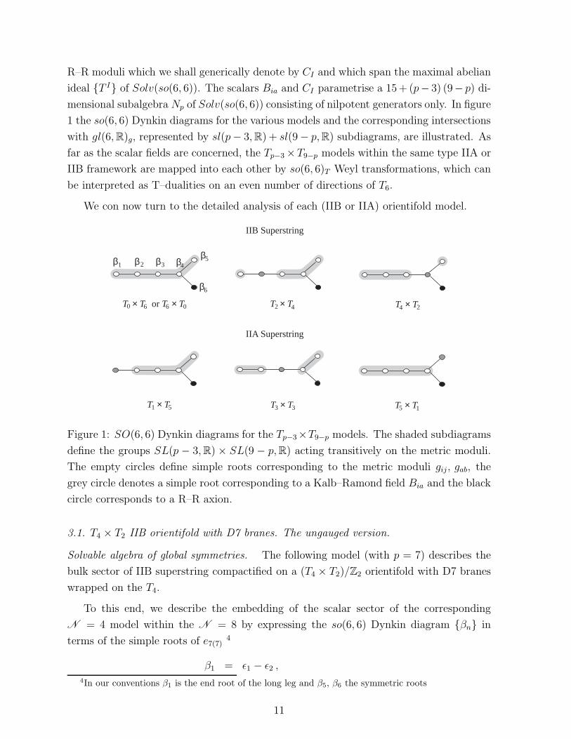
mensional subalgebra Np of Solv(so(6, 6)) consisting of nilpotent generators only. In figure

1 the so(6, 6) Dynkin diagrams for the various models and the corresponding intersections

with gl(6,R)g, represented by sl(p− 3,R) + sl(9− p,R) subdiagrams, are illustrated. As

far as the scalar fields are concerned, the Tp−3×T9−p models within the same type IIA or

IIB framework are mapped into each other by so(6, 6)T Weyl transformations, which can

be interpreted as T–dualities on an even number of directions of T6.

We con now turn to the detailed analysis of each (IIB or IIA) orientifold model.

IIB Superstring

IIA Superstring

T × T or T × T0 6 06 2 4T × T 24T × T

1 5T × T 5 1T × T3 3T × T

1β 2β 3β 4β 5β

6β

Figure 1: SO(6, 6) Dynkin diagrams for the Tp−3×T9−p models. The shaded subdiagrams

define the groups SL(p − 3,R)× SL(9 − p,R) acting transitively on the metric moduli.

The empty circles define simple roots corresponding to the metric moduli gij, gab, the

grey circle denotes a simple root corresponding to a Kalb–Ramond field Bia and the black

circle corresponds to a R–R axion.

3.1. T4 × T2 IIB orientifold with D7 branes. The ungauged version.

Solvable algebra of global symmetries. The following model (with p = 7) describes the

bulk sector of IIB superstring compactified on a (T4 × T2)/Z2 orientifold with D7 branes

wrapped on the T4.

To this end, we describe the embedding of the scalar sector of the corresponding

N = 4 model within the N = 8 by expressing the so(6, 6) Dynkin diagram βn in

terms of the simple roots of e7(7)4

β1 = ǫ1 − ǫ2 ,4In our conventions β1 is the end root of the long leg and β5, β6 the symmetric roots

11

β2 = ǫ2 − ǫ3 ,

β3 = ǫ3 − ǫ4 ,

β4 = ǫ4 + ǫ5 ,

β5 = −ǫ5 + ǫ6 ,

β6 = −12(

6∑

n=1

ǫn) +1√2ǫ7 = a .

According to eq. (15), the root β6 corresponds to the ten–dimensional R–R scalar C0,

and thus identifies the type IIB duality group SL(2,R)IIB. The Dynkin diagram of the

external SL(2,R) factor in the isometry group consists, instead, of the single root

β = a + ǫ1 + ǫ2 + ǫ3 + ǫ4 . (28)

It is useful to classify the positive roots according to their grading with respect to three

relevant O(1, 1) groups generated by the Cartan operatorsHβ, Hλ4 , Hλ6 and parametrised

by the moduli β · h, h4, h6:

O(1, 1)0 → eβ·h = V4 ,

O(1, 1)1 → eh4 = (V4)14 (V2)

12 ,

O(1, 1)2 → eh6 = e−φ , (29)

where we have denoted by λn the so(6, 6) simple weights, λn · βm = δnm. O(1, 1)0 is

generated by the Cartan generator of the external SL(2,R) and O(1, 1)1, O(1, 1)2 are

in GL(4,R) × GL(2,R), the former corresponding to the metric modulus given in eq.

(27). In table 5 we list the axionic fields of the model together with the corresponding

generator of Solv(sl(2,R)) + Solv(so(6, 6)), for each of which the O(1, 1)3 grading and

the SL(4,R) × SL(2,R) representations are specified. The indices i, j and a, b label as

usual the directions of the torus which are longitudinal (T4) and transverse (T2) to the

D–branes.

The fields Bia and Cia transform in the representation (4, 4) of SL(4,R) × SO(2, 2)

where SO(2, 2) = SL(2,R)×SL(2,R)IIB, and therefore will be collectively denoted by Φλi ,

where λ = (α, a) = 1, 2, 3, 4 labels the 4 of SO(2, 2), with a choice of basis corresponding

to the invariant metric ηλσ = diag(+1, +1, −1, −1). Its expression in terms of the fields

Bia and Cia is

Φλi = 1√

2Ci2 − Bi1, Bi2 + Ci1, Bi1 + Ci2, −Bi2 + Ci1 . (30)

We shall use the same notation for the corresponding generators, T iλ ≡ T 1ia, T 2ia.

From the assigned gradings one can conclude that the generators T0, Tiλ and T ij close

a 23–dimensional nilpotent solvable subalgebra N7 of Solv(so(6, 6)). The non–trivial

12

Table 5: Axionic fields for the T4×T2 IIB orientifold, generators of Solv(so(6, 6)), O(1, 1)3

gradings, and SL(4,R)× SL(2,R) representations.

GL(4)×GL(2)–rep. generator root field dim.

— T(0,0,0) ǫi − ǫj , ǫa − ǫb (i < j, a > b) gij , gab 7

(1,1)(0,0,1) T0 a C0 1

(4,2)(0,1,0) T 1ia ǫi + ǫa Bia 8

(4,2)(0,1,1) T 2ia a+ ǫi + ǫa Cia 8

(6,1)(0,2,1) T ij a+ (ǫi + ǫa) + (ǫj + ǫb) Cij ab ≡ Cij ǫab 6

(1,1)(2,0,0) T β = a+ ǫ1 + ǫ2 + ǫ3 + ǫ4 Cijkl ≡ c 1

commutation relations are determined by the grading and the index structure of the

generators, and read

[T0, T

iλ

]= Mλ

λ′

T iλ′ ,

[T iλ, T

jλ′

]= ηλλ′ T ij . (31)

where Mλλ′

is a nilpotent generator acting on the 4 of SO(2, 2) which, for our choice of

basis, can be cast in the form

Mλλ′

= 12

0 −1 0 −1

1 0 1 0

0 1 0 1

−1 0 −1 0

. (32)

Infinitesimal transformations. Let us consider now the infinitesimal transformations of

the scalar fields generated by T0, Tλi and Tij . For simplicity we shall restrict our analysis

to those points in the moduli space where the only non-vanishing scalars are Φλi , C

ij and

C. The corresponding coset representative thus takes the simple form

L = exp(Cij T

ij)exp

(Φλi T

iλ

)exp (C T0) , (33)

and its associated left–invariant one–form is

L−1dL = (L−1∂0L) dC + (L−1∂iλL) dΦ

λi + (L−1∂ijL) dCij

= T0 dC + dΦλi (δ

λ′

λ − CMλλ′

) T iλ′ + 1

2T ij dΦλ

i Φλj + T ij dCij . (34)

In general, the action of an element TΛ on the coset representative can be expressed as:

L−1TΛL = kαΛL

−1∂αL , (35)

13

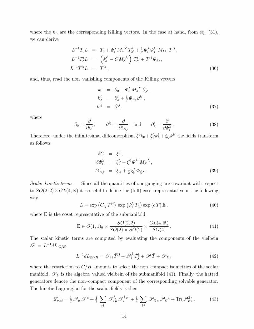
where the kΛ are the corresponding Killing vectors. In the case at hand, from eq. (31),

we can derive

L−1T0L = T0 + Φλi Mλ

λ′

T iλ′ + 1

2Φλi Φ

λ′

j Mλλ′ T ij ,

L−1T iλL =

(

δλ′

λ − CMλλ′

)

T iλ′ + T ij Φjλ ,

L−1T ijL = T ij , (36)

and, thus, read the non–vanishing components of the Killing vectors

k0 = ∂0 + Φλi Mλ

λ′

∂iλ′ ,

kiλ = ∂i

λ +12Φjλ ∂

ij ,

kij = ∂ij , (37)

where

∂0 =∂

∂C, ∂ij =

∂

∂Cijand ∂i

λ =∂

∂Φλi

. (38)

Therefore, under the infinitesimal diffeomorphism ξ0k0+ ξλi kiλ+ ξijk

ij the fields transform

as follows:

δC = ξ0 ,

δΦλi = ξλi + ξ0 Φλ′

Mλ′

λ ,

δCij = ξij +12ξλ[i Φj]λ . (39)

Scalar kinetic terms. Since all the quantities of our gauging are covariant with respect

to SO(2, 2)×GL(4,R) it is useful to define the (full) coset representative in the following

way

L = exp(Cij T

ij)exp

(Φλi T

iλ

)exp (c T )E , (40)

where E is the coset representative of the submanifold

E ∈ O(1, 1)0 ×SO(2, 2)

SO(2)× SO(2)× GL(4,R)

SO(4). (41)

The scalar kinetic terms are computed by evaluating the components of the vielbein

P = L−1dL|G/H :

L−1dL|G/H = Pı Tı + P

λı T

ıλ+ P T + PE , (42)

where the restriction to G/H amounts to select the non–compact isometries of the scalar

manifold, PE is the algebra–valued vielbein of the submanifold (41). Finally, the hatted

generators denote the non–compact component of the corresponding solvable generator.

The kinetic Lagrangian for the scalar fields is then

Lscal =12Pµ P

µ + 12

∑

ıλ

Pλı µ P

λ µı + 1

4

∑

ı

Pı µ Pıµ + Tr(P2

E) , (43)

14

where

Pµ = ∂µc ,

Pλıµ = (∂µΦ

λi )E

iı Eλ

λ ,

Pıµ =[∂µCij +

14(∂µΦ

λi Φjλ − ∂µΦ

λj Φiλ)

]Ei

ı Ej . (44)

Vector fields. The twelve vector potentials are Baµ, Caµ, Giµ, Cijkµ. As before, we

shall collectively denote by Aλµ the pair Baµ, Caµ, and by F λ = dAλ the corresponding

field strengths. To avoid confusion, we shall then adopt the following notation for the

remaining field strengths: F i = dGi and F i = ǫijkl dCjkl. Moreover, Fλ, Fi and Fi will

denote the “dual” field strengths, obtained by varying the Lagrangian with respect to the

electric ones, not to be confused with the four–dimensional Hodge duals ∗F λ, ∗F i and∗F i. Following [37], we can then collect the field strengths and their duals in a symplectic

vector

F λ, Fi, F i, Fλ, Fi, Fi . (45)

In table 6, we list the field strengths and their duals as they appear in the symplectic

section, together with their O(1, 1)3 gradings and the corresponding weights of the 56 of

E7(7).

Table 6: Field strengths, O(1, 1)3 gradings, and corresponding weights.

Sp–section O(1, 1)3–grading weight

F1a (−1, 0,−12) ǫa − 1√

2ǫ7

F2a (−1, 0, 12) w + ǫa

F i (−1,−1,−12) −ǫi − 1√

2ǫ7

F i (1,−1,−12) w + ǫj + ǫk + ǫl

F 1a (1, 0, 12) −ǫa +

1√2ǫ7

F 2a (1, 0,−12) −w − ǫa

Fi (1, 1, 12) ǫi +

1√2ǫ7

Fi (−1, 1, 12) −w − ǫj − ǫk − ǫl

Under a generic nilpotent transformation

ξT + ξ0 T0 + ξλi Tiλ + ξijT

ij , (46)

the field strengths transform as

δF λ = −ξλi Fi + ξ0 F

λ′

Mλ′

λ ,

15

δF i = 0 ,

δF i = ξ Fi ,

δFλ = ξ ηλλ′ F λ′ − ξ0Mλλ′

Fλ′ − ηλλ′ ξλ′

i F i ,

δFi = −ξ Fi + ξλi Fλ − 2 ξij Fj ,

δFi = −ξλ′

i F λ ηλλ′ + 2 ξij Fj . (47)

We then deduce that the electric subalgebra is

ge = o(1, 1)(0,0) + so(2, 2)(0,0) + gl(4,R)(0,0) + (1, 1)(2,0) + (4, 4)(0,1) + (1, 6)(0,2) , (48)

where o(1, 1)(0,0) is the generator of O(1, 1)0, and the grading refers to O(1, 1)0×O(1, 1)1.

The group O(1, 1)2 is now included inside SO(2, 2) and, in what follows, we shall not

consider its grading any longer. Furthermore, we identify T as the generator in (1, 1)(2,0),

T iλ and T ij are associated to (4, 4)(0,1) and (6, 1)(0,2), respectively. The interested reader

may find in appendix the explicit symplectic realisation of the generators of N7, as well

as the computation of the vector kinetic matrix.

3.2. T2 × T4 IIB orientifold with D5 branes. The ungauged version

Solvable algebra of global symmetries. In this second model the relevant axions are

Bia, Cab, Ciabc ≡ Cdi , Cµν ≡ c and Cij = ǫij c

′, and can be associated to the following

choice of simple roots

β1 = ǫ1 − ǫ2 ,

β2 = ǫ2 + ǫ3 ,

β3 = −ǫ3 + ǫ4 ,

β4 = −ǫ4 + ǫ5 ,

β5 = −ǫ5 + ǫ6 ,

β6 = a+ ǫ3 + ǫ4 ,

for the subalgebra so(6, 6) ⊂ e7(7). The Dynkin diagram of the external SL(2,R) consists,

instead, of the single root

β = a+ ǫ1 + ǫ2 , (49)

whose corresponding axion is Cij , according to eq. (15).

The triple grading, this time, refers to the O(1, 1)3 group generated by the three

Cartan Hβ, Hλ2 , Hλ6 and parametrised by the moduli β · h, h2, h6:

O(1, 1)0 → eβ·h = V2 e−φ

2 ,

O(1, 1)1 → eh2 = (V2)12 (V4)

14 e

φ2 ,

O(1, 1)2 → eh6 = (V4)12 e−

φ2 , (50)

16

where, as usual, O(1, 1)0 is in the external SL(2,R), while O(1, 1)1 and O(1, 1)2 are

contained in GL(2,R)×GL(4,R).

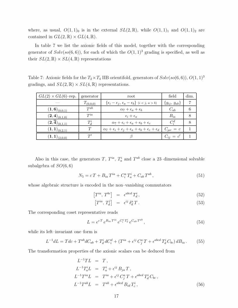
In table 7 we list the axionic fields of this model, together with the corresponding

generator of Solv(so(6, 6)), for each of which the O(1, 1)3 grading is specified, as well as

their SL(2,R)× SL(4,R) representations

Table 7: Axionic fields for the T2×T4 IIB orientifold, generators of Solv(so(6, 6)), O(1, 1)3

gradings, and SL(2,R)× SL(4,R) representations.

GL(2) ×GL(6)–rep. generator root field dim.

— T(0,0,0) ǫi − ǫj , ǫa − ǫb (i < j, a > b) gij , gab 7

(1,6)(0,0,1) T ab α7 + ǫa + ǫb Cab 6

(2,4)(0,1,0) T ia ǫi + ǫa Bia 8

(2,4)(0,1,1) T id α7 + ǫi + ǫa + ǫb + ǫc Cd

i 8

(1,1)(0,2,1) T α7 + ǫi + ǫj + ǫa + ǫb + ǫc + ǫd Cµν = c 1

(1,1)(2,0,0) T ′ β Cij = c′ 1

Also in this case, the generators T , T ia, T ia and T ab close a 23–dimensional solvable

subalgebra of SO(6, 6)

N5 = c T +Bia Tia + Ca

i Tia + Cab T

ab , (51)

whose algebraic structure is encoded in the non–vanishing commutators

[T ia, T bc

]= ǫabcd T i

d , (52)[T ia, T j

d

]= ǫij δad T . (53)

The corresponding coset representative reads

L = ec T eBia T ia

eCai T i

a eCab Tab

, (54)

while its left–invariant one–form is

L−1dL = Tdc+ T abdCab + T id dC

di + (T ia + ǫij Ca

j T + ǫabcd T id Cbc) dBia . (55)

The transformation properties of the axionic scalars can be deduced from

L−1TL = T ,

L−1T iaL = T i

a + ǫij Bja T ,

L−1T iaL = T ia + ǫij Caj T + ǫabcd T i

d Cbc ,

L−1T abL = T ab + ǫabcd Bid Tic , (56)

17

which identify the Killing vectors

k = ∂ ,

kia = ∂i

a + ǫijBja∂ ,

kia = ∂ia ,

kab = ∂ab + ǫabcdBid∂ic , (57)

where

∂ =∂

∂c, ∂i

a =∂

∂Cai

, ∂ia =∂

∂Bia

, ∂ab =∂

∂Cab

. (58)

Hence, under the infinitesimal diffeomorphism ξ T + ξia Tia + ξai T

ia + ξab T

ab, one has

δc = ǫij ξai Bja + ξ ,

δCai = ǫabcd ξbcBid + ξai ,

δBia = ξia ,

δCab = ξab . (59)

For later convenience we shall define the generator Tab = −14ǫabcd T

cd, and the correspond-

ing parameter ξab = −14ǫabcd ξ

cd, in terms of which the relation (52) reads

[Tab, T

ic]= δc[a T

ib] . (60)

Vector fields. The vector fields of this model are Giµ, CiµBaµ, C

aµ, and we name the

corresponding field strengths and their duals by

Fiµν , Fiµν , Haµν , F

aµν , Fiµν , F

iµν , H

aµν , Faµν . (61)

In the table 8 we list the field strengths and their duals as they appear in the symplectic

section, together with their O(1, 1)3 gradings, and the corresponding E7(7) weights.

The transformation laws under a generic nilpotent transformation ξ′ T ′+ξ T+ξab Tab+

ξia Tia + ξai T

ia can be deduced from the grading and weight structures. One finds

δF i = 0 ,

δFi = ξ′ ǫij Fj ,

δHa = ξia Fi ,

δF a = ξab Hb − ξai Fi ,

δFi = ξ′ ǫij Fj + ξai Fa − ξia H

a + ξ Fi ,

δF i = ǫij ξja Fa − ǫij ξaj Ha + ξ F

i

δH a = ξ′ F a + ξab Fb + ξai ǫij Fj ,

δFa = ξ′ Ha − ξai ǫij Fj . (62)

18

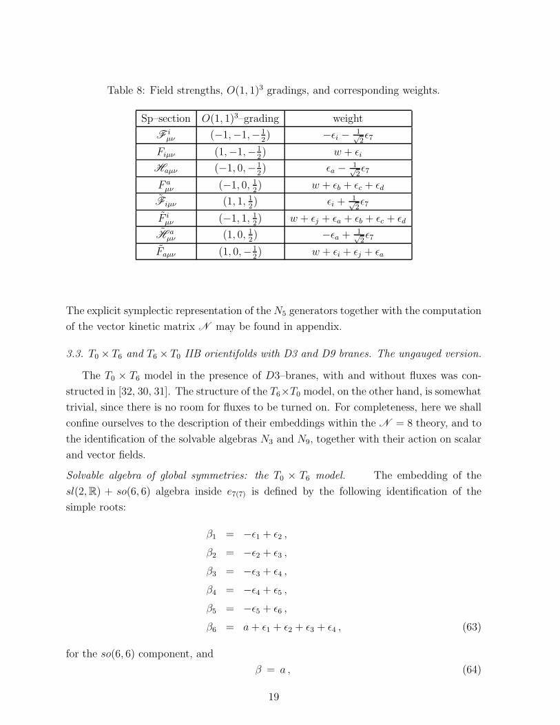
Table 8: Field strengths, O(1, 1)3 gradings, and corresponding weights.

Sp–section O(1, 1)3–grading weight

F iµν (−1,−1,−1

2) −ǫi − 1√

2ǫ7

Fiµν (1,−1,−12) w + ǫi

Haµν (−1, 0,−12) ǫa − 1√

2ǫ7

F aµν (−1, 0, 1

2) w + ǫb + ǫc + ǫd

Fiµν (1, 1, 12) ǫi +

1√2ǫ7

F iµν (−1, 1, 1

2) w + ǫj + ǫa + ǫb + ǫc + ǫd

H aµν (1, 0, 1

2) −ǫa +

1√2ǫ7

Faµν (1, 0,−12) w + ǫi + ǫj + ǫa

The explicit symplectic representation of the N5 generators together with the computation

of the vector kinetic matrix N may be found in appendix.

3.3. T0 × T6 and T6 × T0 IIB orientifolds with D3 and D9 branes. The ungauged version.

The T0 × T6 model in the presence of D3–branes, with and without fluxes was con-

structed in [32, 30, 31]. The structure of the T6×T0 model, on the other hand, is somewhat

trivial, since there is no room for fluxes to be turned on. For completeness, here we shall

confine ourselves to the description of their embeddings within the N = 8 theory, and to

the identification of the solvable algebras N3 and N9, together with their action on scalar

and vector fields.

Solvable algebra of global symmetries: the T0 × T6 model. The embedding of the

sl(2,R) + so(6, 6) algebra inside e7(7) is defined by the following identification of the

simple roots:

β1 = −ǫ1 + ǫ2 ,

β2 = −ǫ2 + ǫ3 ,

β3 = −ǫ3 + ǫ4 ,

β4 = −ǫ4 + ǫ5 ,

β5 = −ǫ5 + ǫ6 ,

β6 = a+ ǫ1 + ǫ2 + ǫ3 + ǫ4 , (63)

for the so(6, 6) component, and

β = a , (64)

19

for the sl(2,R) one. The correspondence axion–root is quite simple and is summarised in

table 9.

Table 9: Axionic fields for the T0×T6 IIB orientifold, generators of Solv(so(6, 6)), O(1, 1)2

gradings and GL(6,R) representations.

GL(6)–rep. generator root field dim.

— T(0,0) ǫa − ǫb (a > b) gab 15

15(0,1) Tab a+ ǫc + ǫd + ǫe + ǫf Cab ≡ ǫabcdef Ccdef 15

1(2,0) T β C0 = c 1

In this case, the grading is with respect to the pair of O(1, 1) groups generated by

Hβ, Hλ6 and corresponding to the following moduli:

O(1, 1)0 → eβ·h = e−φ ,

O(1, 1)1 → eλ6·h = V6 . (65)

The nilpotent algebra N3, generated by Tab, acts as Peccei–Quinn translations on the R–R

scalars Cab

δCab = ξab . (66)

The vector fields are Caµ and Baµ, and the symplectic section of the corresponding

field strengths Faµν and Haµν and their magnetic duals F aµν , H a

µν is listed in table 10.

Table 10: Field strengths, O(1, 1)2 gradings, and corresponding weights.

Sp–section O(1, 1)2–grading weight

Faµν (1,−12) w + ǫa

Haµν (−1,−12) ǫa − 1√

2ǫ7

F aµν (−1, 1

2) −w − ǫa

H aµν (1, 1

2) −ǫa +

1√2ǫ7

The duality action of an infinitesimal transformation ξab Tab + ξ T is then

δFa = ξ Ha ,

20

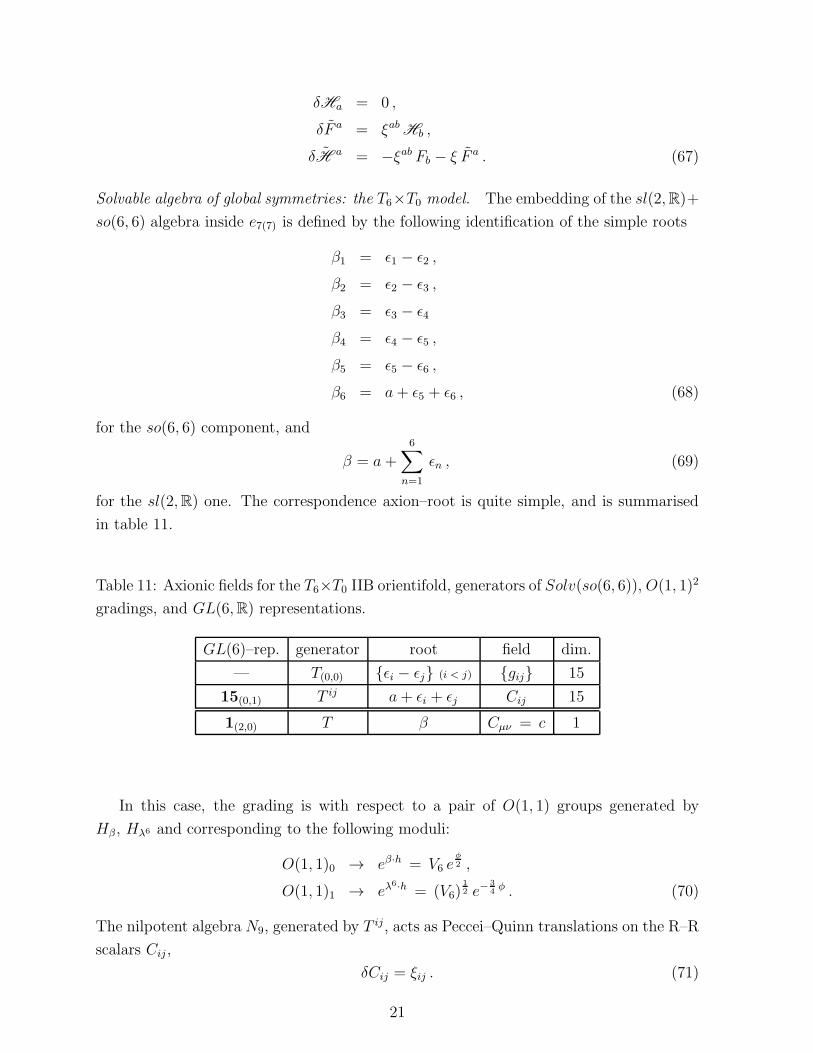
δHa = 0 ,

δF a = ξab Hb ,

δH a = −ξab Fb − ξ F a . (67)

Solvable algebra of global symmetries: the T6×T0 model. The embedding of the sl(2,R)+

so(6, 6) algebra inside e7(7) is defined by the following identification of the simple roots

β1 = ǫ1 − ǫ2 ,

β2 = ǫ2 − ǫ3 ,

β3 = ǫ3 − ǫ4

β4 = ǫ4 − ǫ5 ,

β5 = ǫ5 − ǫ6 ,

β6 = a+ ǫ5 + ǫ6 , (68)

for the so(6, 6) component, and

β = a+

6∑

n=1

ǫn , (69)

for the sl(2,R) one. The correspondence axion–root is quite simple, and is summarised

in table 11.

Table 11: Axionic fields for the T6×T0 IIB orientifold, generators of Solv(so(6, 6)), O(1, 1)2

gradings, and GL(6,R) representations.

GL(6)–rep. generator root field dim.

— T(0,0) ǫi − ǫj (i < j) gij 15

15(0,1) T ij a+ ǫi + ǫj Cij 15

1(2,0) T β Cµν = c 1

In this case, the grading is with respect to a pair of O(1, 1) groups generated by

Hβ, Hλ6 and corresponding to the following moduli:

O(1, 1)0 → eβ·h = V6 eφ2 ,

O(1, 1)1 → eλ6·h = (V6)

12 e−

34φ . (70)

The nilpotent algebra N9, generated by T ij, acts as Peccei–Quinn translations on the R–R

scalars Cij ,

δCij = ξij . (71)

21

The vector fields are Ciµ and Giµ, and the symplectic sections of the corresponding

field strengths Fiµν and F iµν and their magnetic duals F i

µν , Fiµν are listed in table 12.

Table 12: Field strengths, O(1, 1)2 gradings, and corresponding weights.

Sp–section O(1, 1)2–grading weight

Fiµν (−1, 12) w + ǫi

F iµν (−1,−1

2) −ǫi − 1√

2ǫ7

F iµν (1,−1

2) −w − ǫi

Fiµν (1, 12) ǫi +

1√2ǫ7

The duality action of an infinitesimal transformation ξij Tij + ξ T is then

δFi = ξij Fj ,

δF i = 0 ,

δF i = ξ Fi ,

δFi = ξij Fj + ξ Fi . (72)

As a result, the electric group contains the whole SO(6, 6), as for the heterotic string

on T6. In other words, there are no Peccei–Quinn isometries in SO(6, 6) which could be

gauged. This feature is consistent with the fact that this model does not allow fluxes, and

usually fluxes translate into local Peccei–Quinn invariances in the low–energy supergravity

description.

3.4. T1 × T5 IIA orientifold with D4–branes.

Solvable algebra of global symmetries. The embedding of the sl(2,R) + so(6, 6) algebra

inside e7(7) is defined by the following identifications of simple roots:

β1 = ǫ1 + ǫ2 ,

β2 = −ǫ2 + ǫ3 ,

β3 = −ǫ3 + ǫ4 ,

β4 = −ǫ4 + ǫ5 ,

β5 = −ǫ5 + ǫ6 ,

β6 = a+ ǫ2 + ǫ3 + ǫ4 ,

(73)

22

for the so(6, 6) factor, and

β = a + ǫ1 , (74)

for the sl(2,R) one. The correspondence axion–root is quite simple, and is summarised

in table 13.

Table 13: Axionic fields for the T1 × T5 IIA orientifold, generators of Solv(so(6, 6)),

O(1, 1)3 gradings, and GL(5,R) representations.

GL(5)–rep. generator root field dim.

— T(0,0,0) ǫa − ǫb (a > b) gab 10

10(0,0,1) Tab a+ ǫc + ǫd + ǫe Ccde ≡ Cab 10

5(0,1,0) T a ǫ1 + ǫa B1a ≡ Ba 5

5(0,1,1) Te a + ǫ1 + ǫa + ǫb + ǫc + ǫd Cµνa ≡ Ce 5

1(2,0,0) T β C1 = c 1

In this case the grading is with respect to the O(1, 1)3 group generated byHβ, Hλ1, Hλ6

and parametrised by the moduli β · h, h1, h6:

O(1, 1)0 → eβ·h = V1 e− 3

4φ ,

O(1, 1)1 → eh1 = V1 (V5)15 e

φ2 ,

O(1, 1)2 → eh6 = (V5)32 e−

φ4 . (75)

The generators T a, Ta and Tab close a twenty–dimensional nilpotent subalgebra N4 of

Solv(so(6, 6)):

N4 = Ba Ta + Ca Ta + Cab Tab , (76)

whose algebraic structure is encoded in the non–vanishing commutator

[Tab, Tc] = T[aδ

cb] . (77)

The corresponding coset representative reads

L = eCa Ta eBa Ta

eCab Tab ec T E , (78)

where the E factor parametrises the submanifold:

O(1, 1)0 × O(1, 1)1 × O(1, 1)2 ×SL(5,R)

SO(5). (79)

23

A generic element ξa Ta+ ξa Ta+ ξab Tab of N4 then induces the following transformations

on the axionic scalars

δCa = ξa + ξab Bb ,

δBa = ξa ,

δCab = ξab . (80)

Vector fields. The vector fields of this model are Cµ, G1µ, C1aµ, Baµ, and we name the

corresponding field strengths Fµν , F 1µν , F1aµν , Haµν . The symplectic section of the field

strengths and their duals is

Fµν , F1µν , F1aµν , Haµν , Fµν , F1µν , F

1aµν , H

aµν , (81)

and in table 14 we give their O(1, 1)3 gradings and the corresponding E7(7) weights.

Table 14: Field strengths, O(1, 1)3 gradings, and corresponding weights.

vector O(1, 1)3–grading weight

Fµν (1,−1,−12) w

F 1µν (−1,−1,−1

2) −ǫ1 − 1√

2ǫ7

F1aµν (1, 0,−12) w + ǫ1 + ǫa

Haµν (−1, 0,−12) ǫa − 1√

2ǫ7

Fµν (−1, 1, 12) −w

F1µν (1, 1, 12) ǫ1 +

1√2ǫ7

F 1aµν (−1, 0, 1

2) −w − ǫ1 − ǫa

H aµν (1, 0, 1

2) −ǫa +

1√2ǫ7

The action of infinitesimal duality transformation ξa Ta + ξa Ta + ξab Tab + ξ T on the

symplectic section is

δF = ξ F1 ,

δF 1 = 0 ,

δF1a = ξa F + ξ Ha ,

δHa = ξa F1 ,

δF = −ξa F1a + ξa Ha ,

δF1 = −ξa Ha − ξa F1a − ξ F ,

24

δF 1a = −ξa F1 − ξab Hb ,

δH a = ξa F + ξab F1b − ξF 1a . (82)

The explicit symplectic realisation of the N4 generators together with the computation of

the vector kinetic matrix can be found in appendix.

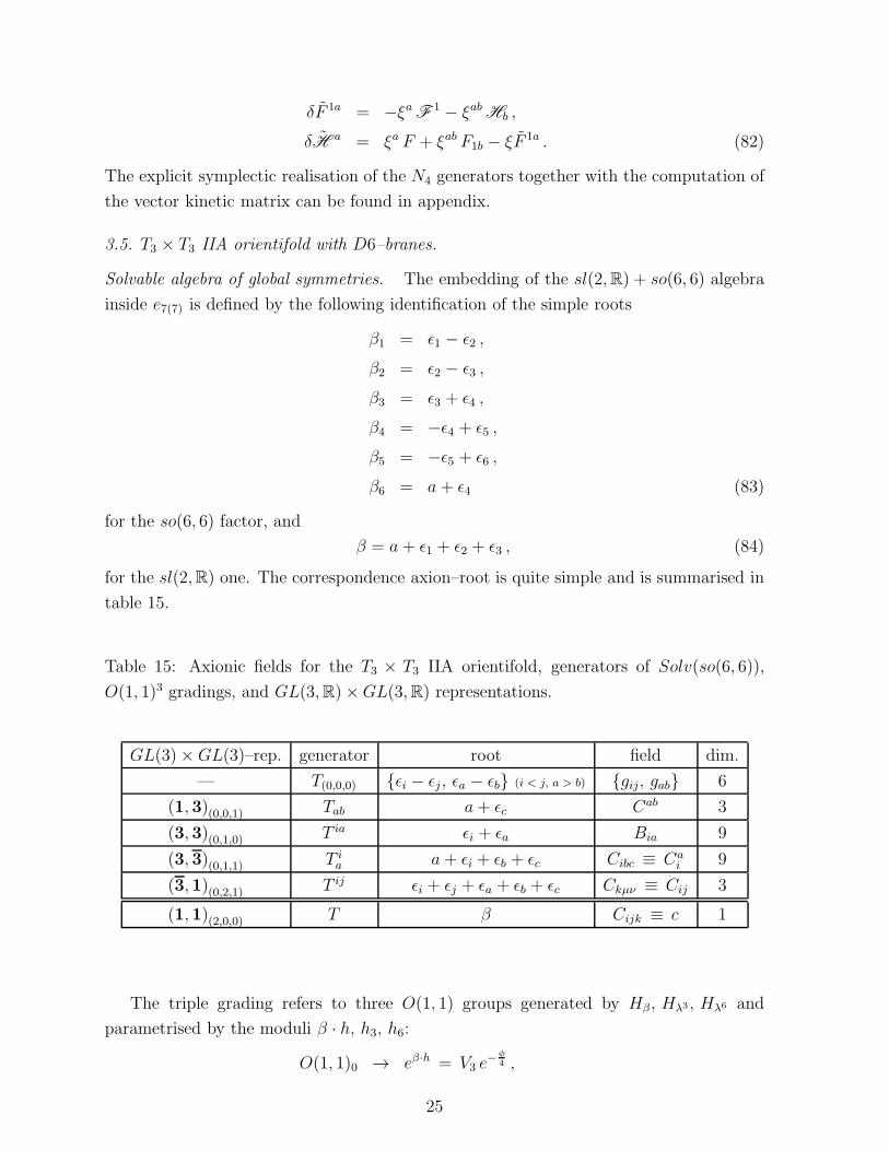
3.5. T3 × T3 IIA orientifold with D6–branes.

Solvable algebra of global symmetries. The embedding of the sl(2,R) + so(6, 6) algebra

inside e7(7) is defined by the following identification of the simple roots

β1 = ǫ1 − ǫ2 ,

β2 = ǫ2 − ǫ3 ,

β3 = ǫ3 + ǫ4 ,

β4 = −ǫ4 + ǫ5 ,

β5 = −ǫ5 + ǫ6 ,

β6 = a + ǫ4 (83)

for the so(6, 6) factor, and

β = a + ǫ1 + ǫ2 + ǫ3 , (84)

for the sl(2,R) one. The correspondence axion–root is quite simple and is summarised in

table 15.

Table 15: Axionic fields for the T3 × T3 IIA orientifold, generators of Solv(so(6, 6)),

O(1, 1)3 gradings, and GL(3,R)×GL(3,R) representations.

GL(3)×GL(3)–rep. generator root field dim.

— T(0,0,0) ǫi − ǫj , ǫa − ǫb (i < j, a > b) gij, gab 6

(1, 3)(0,0,1) Tab a+ ǫc Cab 3

(3, 3)(0,1,0) T ia ǫi + ǫa Bia 9

(3, 3)(0,1,1) T ia a + ǫi + ǫb + ǫc Cibc ≡ Ca

i 9

(3, 1)(0,2,1) T ij ǫi + ǫj + ǫa + ǫb + ǫc Ckµν ≡ Cij 3

(1, 1)(2,0,0) T β Cijk ≡ c 1

The triple grading refers to three O(1, 1) groups generated by Hβ, Hλ3 , Hλ6 and

parametrised by the moduli β · h, h3, h6:

O(1, 1)0 → eβ·h = V3 e−φ

4 ,

25

O(1, 1)1 → eh3 = (V3)13 (V ′

3)13 e

φ2 ,

O(1, 1)2 → eh6 = (V ′3)

13 e−

34φ . (85)

The generators T ia, Tab, Tia and T ij form now a 24–dimensional solvable subalgebra

N6 of Solv(so(6, 6)):

N6 = Bia Tia + Cab Tab + Ca

i Tia + Cij T

ij , (86)

whose algebraic structure is encoded in the non–vanishing commutators

[Tab, T

ic]

= T i[aδ

cb] ,

[Tia, T

jb

]= T ijδab . (87)

A possible choice for the coset representative is then

L = eCij T ij

eCai T i

a eBia T ia

eCab Tab ec T E , (88)

with E parameterising the submanifold

O(1, 1)0 ×GL(3,R)

SO(3)× GL(3,R)

SO(3). (89)

Under an infinitesimal transformation ξij Tij + ξai T

ia + ξia T

ia+ ξab Tab of N6 the variation

of the axionic scalars is

δCai = ξai + ξab Bib ,

δCij = ξij + ξa[iCaj] ,

δBia = ξia ,

δCab = ξab . (90)

Vector fields. The vector fields of this model are Giµ,C

iµ = ǫijk Cjkµ, Baµ, C

aµ = ǫabc Cbcµ,

and we name the corresponding field strengths F iµν , F

iµν , Haµν , F

aµν . The symplectic

section of the field strengths and their duals is

F iµν , F

iµν , Haµν , F

aµν , Fiµν , Fiµν , H

aµν , Faµν , (91)

and in table 16 we give their O(1, 1)3 gradings and the corresponding E7(7) weights.

The action of an infinitesimal duality transformation ξij Tij+ξai T

ia+ξia T

ia+ξab Tab+ξ T

on the symplectic section is

δF i = 0 ,

δF i = ξ Fi ,

26

Table 16: Field strengths, O(1, 1)3 gradings, and corresponding weights.

Sp–section O(1, 1)3–grading weight

F iµν (−1,−1,−1

2) −ǫi − 1√

2ǫ7

F iµν (1,−1,−1

2) w + ǫj + ǫk

Haµν (−1, 0,−12) ǫa − 1√

2ǫ7

F aµν (−1, 0, 1

2) w + ǫb + ǫc

Fiµν (1, 1, 12) ǫi +

1√2ǫ7

F iµν (−1, 1, 1

2) −w − ǫj − ǫk

H aµν (1, 0, 1

2) −ǫa +

1√2ǫ7

Faµν (1, 0,−12) −w − ǫb − ǫc

δHa = ξia Fi ,

δF a = ξab Hb + ξai Fi ,

δFi = −ξia Ha − ξai Fa − 2 ξij F

j − ξ Fi ,

δFi = ξia Fa + ξai Ha + 2 ξij F

j ,

δH a = ξab Fa + ξai Fi + ξ F a ,

δFa = ξia Fi + ξ Ha . (92)

The explicit symplectic realisation of the N6 generators together with the computation of

the vector kinetic matrix can be found in appendix.

3.6. T5 × T1 IIA orientifold with D8–branes

Solvable algebra of global symmetries. The embedding of the sl(2,R) + so(6, 6) algebra

inside e7(7) is defined by the following identification of the simple roots

β1 = ǫ1 − ǫ2 ,

β2 = ǫ2 − ǫ3 ,

β3 = ǫ3 − ǫ4 ,

β4 = ǫ4 − ǫ5 ,

β5 = ǫ5 + ǫ6 ,

β6 = a+ ǫ5 , (93)

27

for the so(6, 6) factor, and

β = a + ǫ1 + ǫ2 + ǫ3 + ǫ4 + ǫ5 , (94)

for the sl(2,R) one. The correspondence axion–root is quite simple and is summarised in

table 17.

Table 17: Axionic fields for the T5 × T1 IIA orientifold, generators of Solv(so(6, 6)),

O(1, 1)3 gradings, and GL(5,R) representations.

GL(5)–rep. generator root field dim.

— T(0,0,0) ǫi − ǫj , ǫa − ǫb (i < j) gij 10

5(0,0,1) T i a+ ǫi Ci 5

5(0,1,0) T ′i ǫi + ǫ6 Bi6 ≡ Bi 5

10(0,1,1) T ij a+ ǫi + ǫj + ǫ6 Cij6 ≡ Cij 10

1(2,0,0) T β Cµν6 ≡ c 1

The triple grading refers to three O(1, 1) groups generated by Hβ, Hλ5 , Hλ6 , all com-

muting with SL(5,R), and parametrised by the moduli β · h, h5, h6:

O(1, 1)0 → eβ·h = V5 eφ4 ,

O(1, 1)1 → eh5 = (V5)15 V1 e

φ2 ,

O(1, 1)2 → eh6 = (V5)15 e−

34φ . (95)

The generators T ′i, T i and T ij form now a twenty–dimensional solvable subalgebra N8 of

Solv(so(6, 6)):

N8 = Bi6 T′i + Ci T

i + Cij Tij , (96)

whose algebraic structure is encoded in the non–vanishing commutator

[T i, T ′j] = T ij . (97)

A possible choice for the the coset representative is then

L = eCij Tij

eBi6 T′i

eCi Ti

ec T E , (98)

with the E parameterising the submanifold:

O(1, 1)0 × O(1, 1)1 × O(1, 1)2 ×SL(5,R)

SO(5). (99)

28

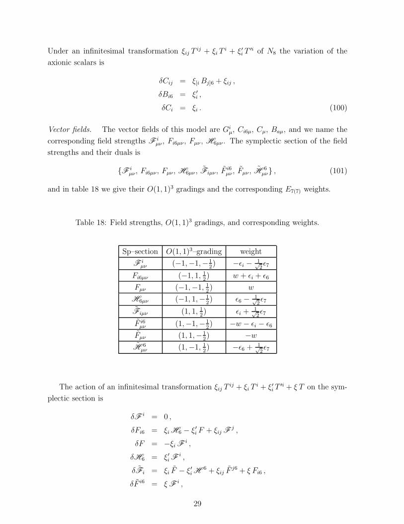
Under an infinitesimal transformation ξij Tij + ξi T

i + ξ′i T′i of N8 the variation of the

axionic scalars is

δCij = ξ[iBj]6 + ξij ,

δBi6 = ξ′i ,

δCi = ξi . (100)

Vector fields. The vector fields of this model are Giµ, Ci6µ, Cµ, Baµ, and we name the

corresponding field strengths F iµν , Fi6µν , Fµν , H6µν . The symplectic section of the field

strengths and their duals is

F iµν , Fi6µν , Fµν , H6µν , Fiµν , F

i6µν , Fµν , H

6µν , (101)

and in table 18 we give their O(1, 1)3 gradings and the corresponding E7(7) weights.

Table 18: Field strengths, O(1, 1)3 gradings, and corresponding weights.

Sp–section O(1, 1)3–grading weight

F iµν (−1,−1,−1

2) −ǫi − 1√

2ǫ7

Fi6µν (−1, 1, 12) w + ǫi + ǫ6

Fµν (−1,−1, 12) w

H6µν (−1, 1,−12) ǫ6 − 1√

2ǫ7

Fiµν (1, 1, 12) ǫi +

1√2ǫ7

F i6µν (1,−1,−1

2) −w − ǫi − ǫ6

Fµν (1, 1,−12) −w

H 6µν (1,−1, 1

2) −ǫ6 +

1√2ǫ7

The action of an infinitesimal transformation ξij Tij + ξi T

i + ξ′i T′i + ξ T on the sym-

plectic section is

δF i = 0 ,

δFi6 = ξi H6 − ξ′i F + ξij Fj ,

δF = −ξi Fi ,

δH6 = ξ′i Fi ,

δFi = ξi F − ξ′i H6 + ξij F

j6 + ξ Fi6 ,

δF i6 = ξ Fi ,

29

δF = ξ′i Fi6 + ξ H6 ,

δH 6 = −ξi Fi6 + ξ F . (102)

The explicit symplectic realisation of the N8 generators, together with the computation

of the vector kinetic matrix can be found in appendix.

4. Fluxes and gauged supergravity: local Peccei–Quinn symmetry as gauged

duality transformations.

In the present section we consider the deformation of N = 4 supergravity induced by

the presence of fluxes. We shall restrict our analysis, here, only to IIB orientifolds with

some (three–form) fluxes turned on, while we shall defer the study of more general fluxes

and of the gauge structure of other models elsewhere.

Differently to what happened in the well–studied T6/Z2 orientifolds, non–abelian

gauged supergravities (for the bulk sector) now emerge, due to the presence of gauge

fields originating from the ten–dimensional metric, and of axionic scalars associated to

the NS–NS two–form B.

4.1. The T4 × T2 IIB orientifold model

In this model, the allowed three–form fluxes are Hλij = Haij , Faij, and are in corre-

spondence with the representation (4, 6)+2 of SO(2, 2)× GL(4,R). The grading simply

counts the number of indices along the internal T4 and, more specifically, is associated to

the subgroup O(1, 1)1 ⊂ GL(4,R). As mentioned in the introduction, inspection of the

dimensionally reduced three–form kinetic term indicates for the four–dimensional theory

a gauge group Gg with connection Ωg = Xi Giµ +XλA

λµ and the following structure:

[Xi, Xj] = HλijXλ . (103)

We may identify the gauge generators with isometries as follows:

Xi = −Hλij T

jλ ,

Xλ = 12Hλ′

ij Tij . (104)

Using relations (31) and the property

Hλk[jHi]ℓλ = 1

2Hλ

ijHkℓλ − 14H ǫijkl , (105)

where H = Hλij H

ijλ , one can show that the generators defined in (104) fulfil the following

algebraic relations

[Xi, Xj ] = Hλij Xλ − 1

4H Tij , (106)

30

which coincide with (103) only if H = 0 which amounts to the condition that∫

T6F(3) ∧

H(3) = 0 (this condition is consistent with a constraint found in [48] on the embedding

matrix of a new gauge group in theN = 8 theory, which seems to yield anN = 8 “lifting”

of the type IIB orientifold models Tp−3 × T9−p discussed here). Under this condition the

gauge group is indeed contained in the isometry group of the scalar manifold. Moreover

it can be verified that under the duality action of the gauge generators defined in (104)

the vector fields transform in the co–adjoint of the gauge group Gg and thus provide a

consistent definition for the gauge connection Ωg . The variation of the gauge potentials

under an infinitesimal transformation with parameters ξλ, ξi reads

δAλµ = ξi Hλ

ij Gjµ + ∂µξ

λ ,

δGiµ = ∂µξ

i ,

δCijkµ = 0 , (107)

and is compatible with the following non–abelian field strengths

F λµν = ∂µA

λν − ∂νA

λµ −Hλ

ij GiµG

jν ,

Fiµν = ∂µG

iν − ∂νG

iµ ,

F iµν = ǫijkl (∂µCjklν − ∂νCjklµ) . (108)

The Cij and Φλi scalars are also charged and, up to rotations, subject to shifts

δCij = 12Hλ

ij ξλ − 12ξk Hλ

k[iΦj]λ,

δΦλi = Hλ

ij ξj , (109)

and their kinetic terms are modified accordingly by covariantisations

DµCij = ∂µCij − 12Hij λ A

λµ +

12Gk

µHλk[iΦj]λ,

DµΦλi = ∂µΦ

λi −Hλ

ij Gjµ . (110)

Chern–Simons terms. The gauge group consists of Peccei–Quinn transformations that

shift the real part of the vector kinetic matrix N (the generalised theta angle). In [49],[50],

it was shown that such a local transformation is a symmetry of the Lagrangian provided

suitable generalised Chern–Simons terms are introduced.

In the case at hand, the new contribution to the Lagrangian is

Lc.s. ∝ ǫµνρσ(

Hλ ij′ Aλµ G

iν ∂ρC

j′

σ + 18Hλ ij′ H

λkℓG

iµC

j′

ν Gkρ G

ℓσ

)

, (111)

corresponding to the non–vanishing entries

Cλ, ij′ = −Hλ ij′ and Ci, λj′ = Hλ ij′ (112)

31

where, in general, the coefficients CΓ,ΛΣ define the moduli–independent gauge variation

of the real part of the kinetic matrix N

δξ ReNΛΣ = ξΓCΓ,ΛΣ . (113)

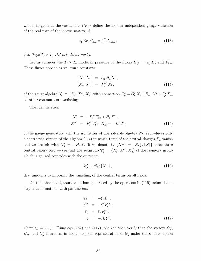
4.2. Type T2 × T4 IIB orientifold model.

Let us consider the T2 × T4 model in presence of the fluxes Hija = ǫij Ha and Fiab.

These fluxes appear as structure constants

[Xi, Xj] = ǫij HaXa ,

[Xi, Xa] = F ab

i Xb , (114)

of the gauge algebra Gg ≡ Xi, Xa, Xa with connection Ωg

µ = GiµXi+Baµ X

a+Caµ Xa,

all other commutators vanishing.

The identification

X ′i = −F ab

i Tab +Ha Tai ,

Xa′ = F abi T i

b , X ′a = −Ha T , (115)

of the gauge generators with the isometries of the solvable algebra N5, reproduces only

a contracted version of the algebra (114) in which three of the central charges Xa vanish

and we are left with X ′a = −Ha T . If we denote by X⊥ = Xa/X ′

a these three

central generators, we see that the subgroup G ′g = X ′

i, Xa′, X ′

a of the isometry group

which is gauged coincides with the quotient:

G′g ≡ Gg/X⊥ , (116)

that amounts to imposing the vanishing of the central terms on all fields.

On the other hand, transformations generated by the operators in (115) induce isom-

etry transformations with parameters:

ξia = −ξi Ha ,

ξab = −ξi F abi ,

ξai = ξb Fbai ,

ξ = −Haξa , (117)

where ξi = ǫij ξj. Using eqs. (62) and (117), one can then verify that the vectors Gi

µ,

Baµ and Caµ transform in the co–adjoint representation of Gg under the duality action

32

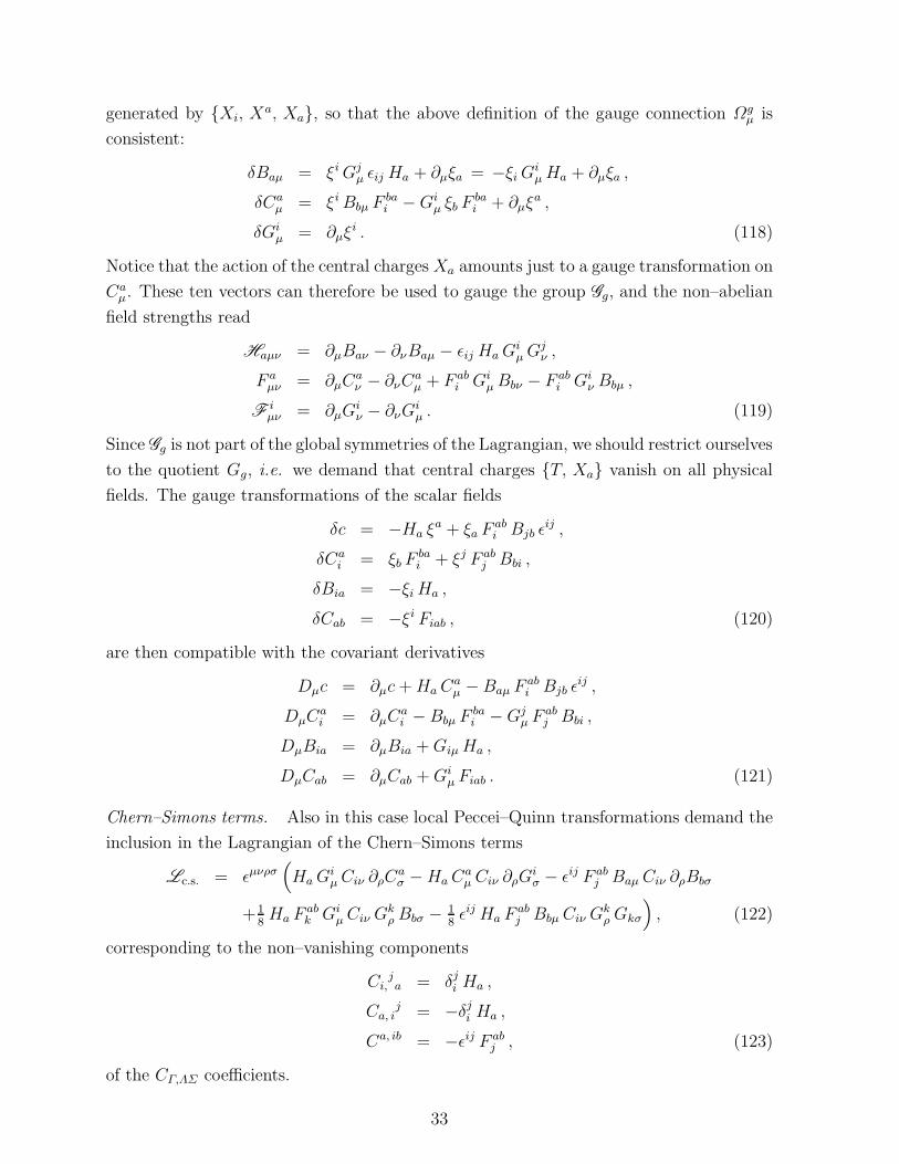
generated by Xi, Xa, Xa, so that the above definition of the gauge connection Ωg

µ is

consistent:

δBaµ = ξiGjµ ǫij Ha + ∂µξa = −ξi G

iµHa + ∂µξa ,

δCaµ = ξiBbµ F

bai −Gi

µ ξb Fbai + ∂µξ

a ,

δGiµ = ∂µξ

i . (118)

Notice that the action of the central charges Xa amounts just to a gauge transformation on

Caµ. These ten vectors can therefore be used to gauge the group Gg, and the non–abelian

field strengths read

Haµν = ∂µBaν − ∂νBaµ − ǫij HaGiµG

jν ,

F aµν = ∂µC

aν − ∂νC

aµ + F ab

i GiµBbν − F ab

i Giν Bbµ ,

Fiµν = ∂µG

iν − ∂νG

iµ . (119)

Since Gg is not part of the global symmetries of the Lagrangian, we should restrict ourselves

to the quotient Gg, i.e. we demand that central charges T, Xa vanish on all physical

fields. The gauge transformations of the scalar fields

δc = −Ha ξa + ξa F

abi Bjb ǫ

ij ,

δCai = ξb F

bai + ξj F ab

j Bbi ,

δBia = −ξi Ha ,

δCab = −ξi Fiab , (120)

are then compatible with the covariant derivatives

Dµc = ∂µc+HaCaµ −Baµ F

abi Bjb ǫ

ij ,

DµCai = ∂µC

ai −Bbµ F

bai −Gj

µ Fabj Bbi ,

DµBia = ∂µBia +GiµHa ,

DµCab = ∂µCab +Giµ Fiab . (121)

Chern–Simons terms. Also in this case local Peccei–Quinn transformations demand the

inclusion in the Lagrangian of the Chern–Simons terms

Lc.s. = ǫµνρσ(

HaGiµCiν ∂ρC

aσ −HaC

aµ Ciν ∂ρG

iσ − ǫij F ab

j Baµ Ciν ∂ρBbσ

+18Ha F

abk Gi

µCiν Gkρ Bbσ − 1

8ǫij Ha F

abj Bbµ Ciν G

kρ Gkσ

)

, (122)

corresponding to the non–vanishing components

Ci,ja = δji Ha ,

Ca, ij = −δji Ha ,

Ca, ib = −ǫij F abj , (123)

of the CΓ,ΛΣ coefficients.

33

5. Conclusions and outlooks

In the present paper, we have investigated the symmetries and the structure of sev-

eral T6 orientifolds which, in absence of fluxes, have N = 4 supersymmetries in four

dimensions. we have not addressed here the question of vacua with some residual su-

persymmetry, that will be the subject of future investigations. All these models lead to

different low–energy supergravity descriptions. When fluxes are turned on, the deformed

Lagrangian is described by a gauged N = 4 supergravity and fermionic mass–terms and

a scalar potential are developed.

The low–energy Lagrangians underlying these orientifolds are different versions of

gauged N = 4 supergravity with six bulk vector multiplets and additional Yang–Mills

multiplets living on the brane world–volume. The gaugings are based on quotients (with

respect to some central charges) of nilpotent subalgebras of so(6, 6). These nilpotent

subalgebras are basically generated by the axion symmetries associated to R–R scalars

and to NS–NS scalars originating from the two–form B–field.

Along similar lines, one can also consider new examples of orientifolds with N = 2, 1

four–dimensional supersymmetries, with and/or without fluxes.

Acknowledgements M.T. would like to thank H. Samtleben for useful discussions and

the Th. Division of CERN, where part of this work has been done, for their kind hos-

pitality. The work of S.F. has been supported in part by European Community’s Hu-

man Potential Program under contract HPRN-CT-2000-00131 Quantum Space-Time, in

association with INFN Frascati National Laboratories and by D.O.E. grant DE-FG03-

91ER40662, Task C. The work of M.T. is supported by a European Community Marie

Curie Fellowship under contract HPRN-CT-2001-01276.

Appendix. Symplectic realisation of the solvable generators

In this appendix, we give the coset representatives of our models in the symplectic

basis of vector fields. This is needed in order to compute the kinetic matrix NΛΣ , which

is a complex symmetric matrix in the space of vectors in the theory. Its imaginary and

real parts describe the terms

ImNΛΣ FΛµνF

Σ µν + 12ReNΛΣ ǫµνρσFΛ

µνFΣρσ . (124)

34

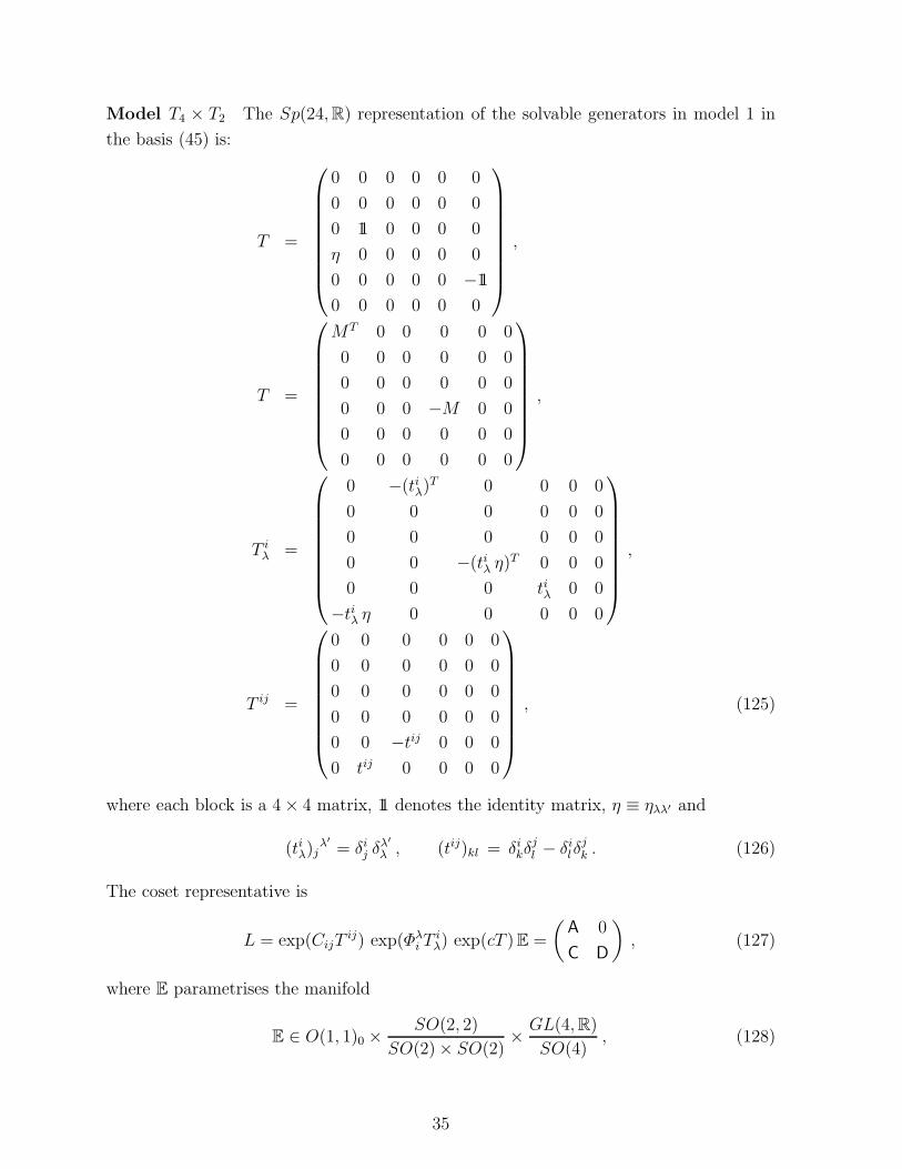
Model T4 × T2 The Sp(24,R) representation of the solvable generators in model 1 in

the basis (45) is:

T =

0 0 0 0 0 0

0 0 0 0 0 0

0 11 0 0 0 0

η 0 0 0 0 0

0 0 0 0 0 −11

0 0 0 0 0 0

,

T =

MT 0 0 0 0 0

0 0 0 0 0 0

0 0 0 0 0 0

0 0 0 −M 0 0

0 0 0 0 0 0

0 0 0 0 0 0

,

T iλ =

0 −(tiλ)T 0 0 0 0

0 0 0 0 0 0

0 0 0 0 0 0

0 0 −(tiλ η)T 0 0 0

0 0 0 tiλ 0 0

−tiλ η 0 0 0 0 0

,

T ij =

0 0 0 0 0 0

0 0 0 0 0 0

0 0 0 0 0 0

0 0 0 0 0 0

0 0 −tij 0 0 0

0 tij 0 0 0 0

, (125)

where each block is a 4× 4 matrix, 11 denotes the identity matrix, η ≡ ηλλ′ and

(tiλ)jλ′

= δij δλ′

λ , (tij)kl = δikδjl − δilδ

jk . (126)

The coset representative is

L = exp(CijTij) exp(Φλ

i Tiλ) exp(cT )E =

(A 0

C D

)

, (127)

where E parametrises the manifold

E ∈ O(1, 1)0 ×SO(2, 2)

SO(2)× SO(2)× GL(4,R)

SO(4), (128)

35

and can be written in the following general form:

E =

e−ϕ E(ℓ) 0 0 0 0 0

0 e−ϕ E 0 0 0 0

0 0 eϕ E 0 0 0

0 0 0 eϕ ηE(ℓ)η 0 0

0 0 0 0 eϕ E−1 0

0 0 0 0 0 e−ϕ E−1

, (129)

with

E(ℓ)λσ ∈ SO(2, 2)

SO(2)× SO(2),

Ei ∈ GL(4,R)

SO(4),

eϕH ∈ O(1, 1)0 , (130)

the hatted indices being the rigid ones transforming under the isotropy group. The blocks

is L read

A =

e−ϕ E(ℓ)λσ −e−ϕ Φλ

i Ei 0

0 e−ϕ Ei 0

0 c e−ϕ Ei eϕ Ei

,

C =

c e−ϕ E(ℓ)λσ −c e−ϕ Φλj Ejı −eϕ Φλj E

jı

c e−ϕ Φδi E(ℓ)δσ −c e−ϕ 2 CijEj

k−eϕ 2 CijEj

k

−e−ϕ Φδi E(ℓ)δσ e−ϕ 2 CijEj

k0

,

D =

eϕ E(ℓ)λσ 0 0

eϕ Φλi E(ℓ)λ

σ eϕ E−1i −c e−ϕ E−1

i

0 0 e−ϕ E−1i

,

Cij = Cij +14Φλi Φλj . (131)

In the sequel we shall need also the expression of A−1:

A−1 =

eϕ E(ℓ)σλ eϕ E(ℓ)

σλΦ

λi 0

0 eϕ E−1 ıj 0

0 −e−ϕ cE−1 ıj e−ϕ E−1 ı

j

. (132)

In terms of the matrices h, f

f = 1√2A , h = 1√

2(C− iD) , (133)

the kinetic matrix is expressed as (see [51] and references therein)

N = hf−1 =

Nλλ′ Nλi N ′λi

∗ Nij N ′ij

∗ ∗ N ′′ij

, (134)

and is characterised by the following entries:

Nλλ′ = −i e2ϕ E(ℓ)λσ E(ℓ)λ′

σ + c ηλλ′ ,

Nλi = −i e2ϕ E(ℓ)λσ E(ℓ)λ′

σ Φλ′

i + c Φλi

N ′λi = −Φλi ,

Nij = −i(

(e2ϕ + e−2ϕ c2)E−1iıE−1

jı + e2ϕ Φλi E(ℓ)λ

σ E(ℓ)λ′

σ Φλ′

j

)

+ c Φλi Φλj ,

N ′ij = i c e−2ϕE−1

iıE−1

jı − 2 Cij ,

N ′′ij = −i e−2ϕ E−1

iıE−1

jı . (135)

36

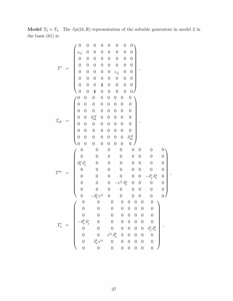
Model T2 × T4 The Sp(24,R) representation of the solvable generators in model 2 in

the basis (61) is:

T ′ =

0 0 0 0 0 0 0 0

ǫij 0 0 0 0 0 0 0

0 0 0 0 0 0 0 0

0 0 0 0 0 0 0 0

0 0 0 0 0 ǫij 0 0

0 0 0 0 0 0 0 0

0 0 0 11 0 0 0 0

0 0 11 0 0 0 0 0

,

Tab =

0 0 0 0 0 0 0 0

0 0 0 0 0 0 0 0

0 0 0 0 0 0 0 0

0 0 δcdab 0 0 0 0 0

0 0 0 0 0 0 0 0

0 0 0 0 0 0 0 0

0 0 0 0 0 0 0 δcdab0 0 0 0 0 0 0 0

,

T ia =

0 0 0 0 0 0 0 0

0 0 0 0 0 0 0 0

δab δij 0 0 0 0 0 0 0

0 0 0 0 0 0 0 0

0 0 0 0 0 0 −δij δab 0

0 0 0 −ǫij δab 0 0 0 0

0 0 0 0 0 0 0 0

0 −δab ǫij 0 0 0 0 0 0

,

T ia =

0 0 0 0 0 0 0 0

0 0 0 0 0 0 0 0

0 0 0 0 0 0 0 0

−δba δij 0 0 0 0 0 0 0

0 0 0 0 0 0 0 δij δba

0 0 ǫij δba 0 0 0 0 0

0 δba ǫij 0 0 0 0 0 0

0 0 0 0 0 0 0 0

,

37

T =

0 0 0 0 0 0 0 0

0 0 0 0 0 0 0 0

0 0 0 0 0 0 0 0

0 0 0 0 0 0 0 0

0 11 0 0 0 0 0 0

11 0 0 0 0 0 0 0

0 0 0 0 0 0 0 0

0 0 0 0 0 0 0 0

. (136)

The coset representative has the form:

L = ec′ T ′

ec T eBia T ia

eCai T i

a eCab Tab

E =

(A 0

C D

)

, (137)

where this time the matrix E describes the submanifold:

E = O(1, 1)0 ×GL(2,R)

SO(2)× GL(4,R)

SO(4), (138)

and has the following form:

E =

e−ϕ E2i 0 0 0 0 0 0 0

0 eϕ E−12 i

0 0 0 0 0 0

0 0 e−ϕ E−14 a

b 0 0 0 0 0

0 0 0 e−ϕ E4ab

0 0 0 0

0 0 0 0 eϕ E−12 i

0 0 0

0 0 0 0 0 e−ϕ E2i 0 0

0 0 0 0 0 0 eϕ E4ab

0

0 0 0 0 0 0 0 eϕ E−14 a

b

, (139)

E2i ∈ GL(2,R)

SO(2),

E4ab ∈ GL(4,R)

SO(4),

eϕH ∈ O(1, 1)0 . (140)

The blocks A, C, D of L can be conveniently described in terms of the following matrices

(B)ia = Bia, (C)ia = Ca

i , (C )ab = Cab:

A =

e−ϕ E2 0 0 0

e−ϕ c′ ǫE2 eϕ E−12 0 0

e−ϕB

t E2 0 e−ϕ E−14 0

−e−ϕ Ct E2 0 e−ϕ C E−14 e−ϕ E4

,

C =

e−ϕ c′ (c ǫ +BCt)E2 −eϕ (c ǫ +BCt) ǫE−12 e−ϕ c′ (C−BC )E−1

4 −e−ϕ c′ BE4

−e−ϕ ǫ (c ǫ+BCt)E2 0 −e−ϕ ǫ (C−BC )E−1

4 e−ϕ ǫBE4

−e−ϕ c′ Ct E2 eϕ Ct ǫ E−12 e−ϕ c′ C E−1

4 e−ϕ c′ E4

e−ϕ c′ Bt E2 −eϕ Bt ǫ E−1

2 e−ϕ c′ E−14 0

,

D =

eϕ E−12 e−ϕ c′ ǫE2 −eϕ BE4 eϕ (C−BC )E−1

4

0 e−ϕ E2 0 0

0 0 eϕ E4 eϕ C E−14

0 0 0 eϕ E−14

, (141)

38

it is also useful to compute A−1:

A−1 =

eϕ E−12 0 0 0

−e−ϕ c′ E2 ǫ e−ϕ E2 0 0

−eϕ E4 Bt 0 eϕ E4 0

eϕ E−14 (C B

t +Ct) 0 −eϕ E−1

4 C eϕ E−14

. (142)

We then compute the kinetic matrix N whose independent components are:

N =

Nij Nij Ni

a Nia

∗ N ij N ia N ia

∗ ∗ Nab Nab

∗ ∗ ∗ Nab

, (143)

where

Nij = −i[E−1

2 iE−1

2 j (e2ϕ + e−2ϕ c′2) + e2ϕBia E4

aaE4

baBjb+

e2ϕ (−Bic Cca + Ca

i )E−14 a

aE−14 b

a (CbdBjd + Cbj )]− 2Ba(i C

aj) c

′ ,

Nij = −i e−2ϕ c′ ǫik E2

kk E2

jk + c δi

j −Bia Cak ǫ

kj ,

Nia = i e2ϕ

[Bib E4

bb E4

ab + (−Bib C

bc + Cci )E

−14 c

c E−14 d

c Cda]+ c′ Ca

i ,

Nia = −i e2ϕ (−Bib Cbc + Cc

i )E−14 c

cE−14 a

c − c′Bia ,

N ij = −i e−2ϕ E2ik E2

jk ,

N ia = −ǫij Caj ,

N ia = ǫij Bja ,

Nab = −i e2ϕ(

−Cad E−14 d

dE−14 c

dCcb + E4ab E4

bb

)

,

Nab = −i e2ϕ CadE−1

4 ddE−1

4 bd + c′ δab ,

Nab = −i e2ϕ E−14 a

dE−14 b

d . (144)

Model T1 × T5 The Sp(24,R) representation of the N4 generators is the following:

T a =

0 0 0 0 0 0 0 0

0 0 0 0 0 0 0 0

δab 0 0 0 0 0 0 0

0 δab 0 0 0 0 0 0

0 0 0 0 0 0 −δab 0

0 0 0 0 0 0 0 −δab0 0 0 0 0 0 0 0

0 0 0 0 0 0 0 0

,

39

Ta =

0 0 0 0 0 0 0 0

0 0 0 0 0 0 0 0

0 0 0 0 0 0 0 0

0 0 0 0 0 0 0 0

0 0 0 δba 0 0 0 0

0 0 −δba 0 0 0 0 0

0 −δba 0 0 0 0 0 0

δba 0 0 0 0 0 0 0

,

Tab =

0 0 0 0 0 0 0 0

0 0 0 0 0 0 0 0

0 0 0 0 0 0 0 0

0 0 0 0 0 0 0 0

0 0 0 0 0 0 0 0

0 0 0 0 0 0 0 0

0 0 0 −δcdab 0 0 0 0

0 0 δcdab 0 0 0 0 0

T =

0 11 0 0 0 0 0 0

0 0 0 0 0 0 0 0

0 0 0 11 0 0 0 0

0 0 0 0 0 0 0 0

0 0 0 0 0 0 0 0

0 0 0 0 −11 0 0 0

0 0 0 0 0 0 0 0

0 0 0 0 0 0 −11 0

. (145)

We have chosen the coset representative to have the form given in eq. (78). We may

choose for the matrix E the following matrix form:

E =

eϕ E 0 0 0 0 0 0 0

0 e−ϕ E 0 0 0 0 0 0

0 0 eϕ E−1ab 0 0 0 0 0

0 0 0 e−ϕ E−1ab 0 0 0 0

0 0 0 0 e−ϕ/E 0 0 0

0 0 0 0 0 eϕ/E 0 0

0 0 0 0 0 0 e−ϕ Eab

0

0 0 0 0 0 0 0 eϕ Eab

, (146)

where:

Eab , E ∈ O(1, 1)1 ×O(1, 1)2 ×

SL(5,R)

SO(5),

eH ϕ ∈ O(1, 1)0 . (147)

The blocks A, C, D of L and A−1 have the following form:

A =

E eϕ c E e−ϕ 0 0

0 E e−ϕ 0 0

Ba E eϕ cBa E e−ϕ eϕ E−1ab c e−ϕ E−1

ab

0 Ba e−ϕ 0 e−ϕ E−1ab

,

40

C =

0 Ba Ca E e−ϕ 0 e−ϕ (Bb Cba + Ca)E−1

ad

−Ba Ca E eϕ −cBa Ca E e−ϕ −eϕ (Bb Cba + Ca)E−1

ad −e−ϕ c (Bb C

ba + Ca)E−1ad

0 −e−ϕ Ca E 0 e−ϕ Cab E−1bd

Ca E eϕ cCa E e−ϕ eϕ Cab E−1bd e−ϕ c Cab E−1

bd

,

D =

e−ϕ/E 0 −Ba e−ϕ Ead

0

−c e−ϕ/E eϕ/E cBa e−ϕ Ead

−Ba eϕ Ead

0 0 e−ϕ Ead

0

0 0 −c e−ϕ Ead

eϕ Ead

,

A−1 =

e−ϕ/E −c e−ϕ/E 0 0

0 eϕ/E 0 0

−e−ϕ Eda Ba c e−ϕ E

da Ba e−ϕ E

da −c e−ϕ E

da

0 −eϕ EdaBa 0 eϕ E

da

, (148)

from equations (133) and (134) we compute the matrix N :

N =

N N1 N (1a) Na

∗ N1 1 N1(1a) N1

a

∗ ∗ N (1a) (1b) N (1a) b

∗ ∗ ∗ Na b

, (149)

whose entries are

N = −i e−2ϕ (BaBb EaaE

ba +

1

E2) ,

N1 = i c e−2ϕ (BaBb EaaE

ba +

1

E2) ,

N (1a) = i e−2ϕ Bb EaaE

ba ,

Na = Ca +Bb Cba − i c e−2ϕ Bb E

aaE

ba ,

N1 1 = −i (e−2ϕ c2 + e2ϕ) (BaBb EaaE

ba +

1

E2) ,

N1(1a) = −(BbC

ba + Ca)− i c e−2ϕ Bb EaaE

ba ,

N1a = i (e−2ϕ c2 + e2ϕ)Bb E

aa E

ba ,

N (1a) (1b) = −i e−2ϕ Eaa E

ba ,

N (1a) b = −Cab + i e−2ϕ cEaaE

ba ,

Na b = −i (e−2ϕ c2 + e2ϕ)EaaE

ba , (150)

where the asterisks denote the symmetric entries.

Model T3 × T3 The Sp(24,R) representation of the N6 generators is the following:

Tab =

0 0 0 0 0 0 0 0

0 0 0 0 0 0 0 0

0 0 0 0 0 0 0 0

0 0 δcdab 0 0 0 0 0

0 0 0 0 0 0 0 0

0 0 0 0 0 0 0 0

0 0 0 0 0 0 0 δcdab0 0 0 0 0 0 0 0

,

41

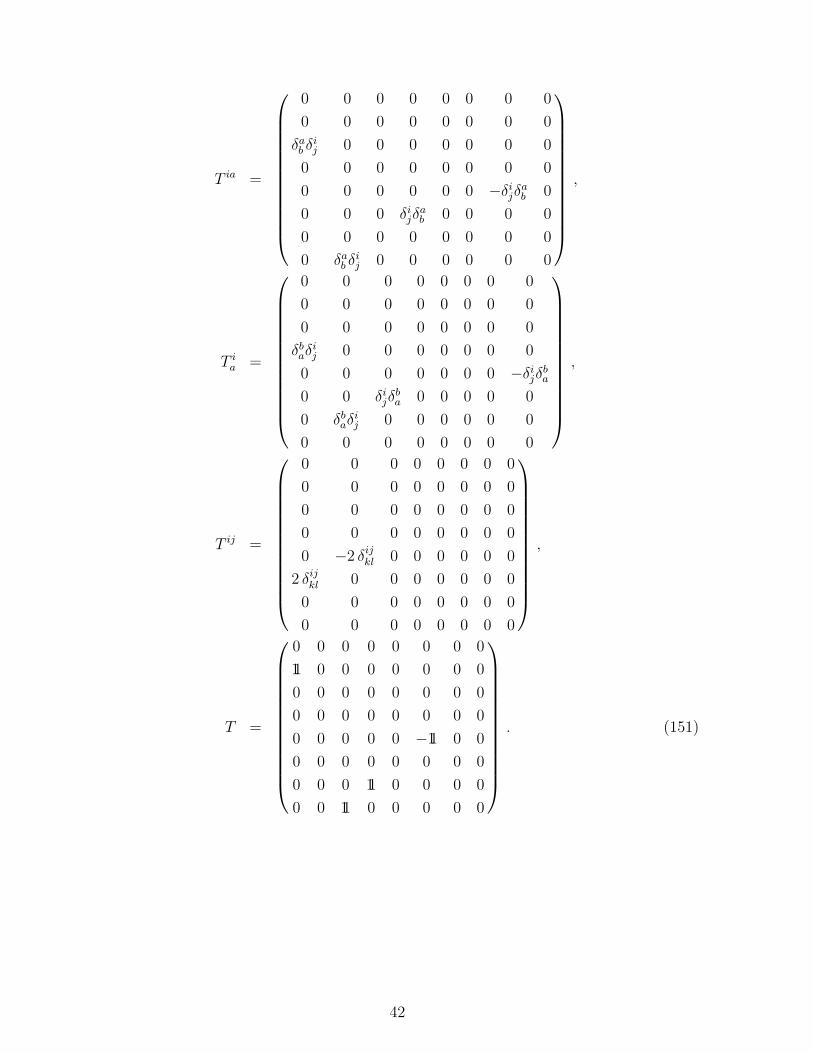
T ia =

0 0 0 0 0 0 0 0

0 0 0 0 0 0 0 0

δab δij 0 0 0 0 0 0 0

0 0 0 0 0 0 0 0

0 0 0 0 0 0 −δijδab 0

0 0 0 δijδab 0 0 0 0

0 0 0 0 0 0 0 0

0 δab δij 0 0 0 0 0 0

,

T ia =

0 0 0 0 0 0 0 0

0 0 0 0 0 0 0 0

0 0 0 0 0 0 0 0

δbaδij 0 0 0 0 0 0 0

0 0 0 0 0 0 0 −δijδba

0 0 δijδba 0 0 0 0 0

0 δbaδij 0 0 0 0 0 0

0 0 0 0 0 0 0 0

,

T ij =

0 0 0 0 0 0 0 0

0 0 0 0 0 0 0 0

0 0 0 0 0 0 0 0

0 0 0 0 0 0 0 0

0 −2 δijkl 0 0 0 0 0 0

2 δijkl 0 0 0 0 0 0 0

0 0 0 0 0 0 0 0

0 0 0 0 0 0 0 0

,

T =

0 0 0 0 0 0 0 0

11 0 0 0 0 0 0 0

0 0 0 0 0 0 0 0

0 0 0 0 0 0 0 0

0 0 0 0 0 −11 0 0

0 0 0 0 0 0 0 0

0 0 0 11 0 0 0 0

0 0 11 0 0 0 0 0

. (151)

42

We have chosen the coset representative to have the form given in eq. (88). We may

choose for the matrix E the following matrix form:

E =

e−ϕ Ei1 0 0 0 0 0 0 0

0 eϕ Ei1 0 0 0 0 0 0

0 0 e−ϕ E−12 a

b 0 0 0 0 0

0 0 0 e−ϕ Ea2 b

0 0 0 0

0 0 0 0 eϕ E−11 i

0 0 0

0 0 0 0 0 e−ϕ E−11 i

0 0

0 0 0 0 0 0 eϕ Ea2 b

0

0 0 0 0 0 0 0 eϕ E−12 a

b

, (152)

where

Ei1 ∈

(GL(3,R)

SO(3)

)

1

,

Ea2 b ∈

(GL(3,R)

SO(3)

)

2

,

eϕH ∈ SO(1, 1)0 . (153)

The blocks A, C, D of L and A−1 have the following form:

A =

e−ϕ Ei1 0 0 0

c e−ϕ Ei1 eϕ Ei

1 0 0

Bia e−ϕ Ei1 0 e−ϕ E−1

2 ab 0

Cai e−ϕ Ei

1 0 e−ϕ Cab E−12 b

c e−ϕ E2ac

,

C =

−2 c e−ϕ Cij Ej1 k

−2 eϕ Cij Ej1 k

−c e−ϕ (Cai + Bib C

ba)E−12 a

c −e−ϕ cBib E−12

bd

2e−ϕ Cij Ej1 k

0 e−ϕ (Cai + Bib C

ba)E−12 a

c e−ϕ Bia E2ac

c e−ϕ Cai Ei

1keϕ Ca

i Ei1k

c e−ϕ Cab E−12 b

c c e−ϕ E2ac

c e−ϕ Bia Ei1k

eϕ Bia Ei1k

c e−ϕ E−12 a

c 0

,

D =

eϕ E−11 i

−c e−ϕ E−11 i

−eϕ Bia Ea2 d

−eϕ (Cai +Bib C

ba)E−12 a

c

0 e−ϕ E−11 i

0 0

0 0 eϕ Ea2 d

eϕ Cab E−12 b

c

0 0 0 eϕ E−12 a

c

,

A−1 =

eϕ E−11

i 0 0 0

−c e−ϕ E−11

i e−ϕ E−1

1i 0 0

−eϕ E2aa Bia 0 eϕ E2a

a 0

−eϕ E−12

ca (Bib C

ba + Cai ) 0 −eϕ E−1

2ca Cab eϕ E−1

2ca

,

Cij = Cij +12Ca

i Bja . (154)

The vector kinetic matrix can now be calculated and has the following form:

N =

Nij N ′ij Ni

a Nia

∗ N ′′ij N ′

ia N ′

ia

∗ ∗ Nab Nab

∗ ∗ ∗ Nab

, (155)

whose entries are

Nij = 2 cBa(i Caj) − i

[(c2 e−2ϕ + e2ϕ)E−1

1 iE−1

1 j+

e2ϕ (Cai + Bib C

ba) (Ccj +BjbC

bc)E−12 a

c E−12 c

c + e2ϕ BiaBjb Ea2 c E

b2 c

],

43

N ′ij = −2 Cij + i c e−2ϕE−1

1 iE−1

1 j ,

Nia = −c Ca

i + i e2ϕ[(Cb

i +BicCcb)CadE−1

2 beE−1

2 de +Bib E

a2 cE

b2 c

],

Nia = −cBia + i e2ϕ (Cbi +BicC

cb)E−12 b

eE−12 a

e ,

N ′′ij = −i e−2ϕ E−1

1 iE−1

1 j

N ′ia = Ca

i ,

N ′ia = Bia ,

Nab = −i e2ϕ[Ea

2 cEb2 c + Cac CbdE−1

2 ce E−1

2 de],

Nab = c− i e2ϕCac E−1

2 ce E−1

2 be ,

Nab = −i e2ϕ E−12 a

e E−12 b

e . (156)

Model T5 × S1 The Sp(24,R) representation of the N8 generators is the following:

T i =

0 0 0 0 0 0 0 0

0 0 0 δij 0 0 0 0

−δij 0 0 0 0 0 0 0

0 0 0 0 0 0 0 0

0 0 0 0 0 0 δij 0

0 0 0 0 0 0 0 0

0 0 0 0 0 0 0 0

0 0 0 0 0 −δij 0 0

,

T ′i =

0 0 0 0 0 0 0 0

0 0 −δij 0 0 0 0 0

0 0 0 0 0 0 0 0

δij 0 0 0 0 0 0 0

0 0 0 0 0 0 0 −δij0 0 0 0 0 0 0 0

0 0 0 0 0 δij 0 0

0 0 0 0 0 0 0 0

,

T ij =

0 0 0 0 0 0 0 0

δijkl 0 0 0 0 0 0 0

0 0 0 0 0 0 0 0

0 0 0 0 0 0 0 0

0 0 0 0 0 δijkl 0 0

0 0 0 0 0 0 0 0

0 0 0 0 0 0 0 0

0 0 0 0 0 0 0 0

,

44

T =

0 0 0 0 0 0 0 0

0 0 0 0 0 0 0 0

0 0 0 0 0 0 0 0

0 0 0 0 0 0 0 0

0 11 0 0 0 0 0 0

11 0 0 0 0 0 0 0

0 0 0 11 0 0 0 0

0 0 11 0 0 0 0 0

. (157)

We have chosen the coset representative to have the form given in eq. (98). We may

choose for the matrix E the following matrix form

E =

e−ϕ Ei 0 0 0 0 0 0 0

0 e−ϕ E−1i 0 0 0 0 0 0

0 0 e−ϕ E 0 0 0 0 0

0 0 0 e−ϕ /E 0 0 0 0

0 0 0 0 eϕ E−1i 0 0 0

0 0 0 0 0 eϕ Ei 0 0

0 0 0 0 0 0 eϕ/E 0

0 0 0 0 0 0 0 eϕ E

, (158)

where:

Ei, E ∈ O(1, 1)1 ×O(1, 1)2 ×

SL(5,R)

SO(5),

eϕH ∈ SO(1, 1)0 . (159)

The blocks A, C, D of L and A−1 have the following form

A = e−ϕ

Ei 0 0 0

(Bi Cj + Cij)Ej E−1

i −Bi E Ci/E

−Ci Ei 0 E 0

Bi Ei 0 0 1/E

,

C = e−ϕ

c (Bi Cj + Cij)Ej cE−1

i −cBi E cCi/E

cEi 0 0 0

cBi Ei 0 0 c/E

−cCi Eik

0 c E 0

,

D = eϕ

E−1i (Bi Cj + Cij)Ej

Ci/E −Bi E

0 Ei 0 0

0 BiEi 1/E 0

0 −CiEi 0 E

,

A−1 = eϕ

E−1i 0 0 0

Eıj (Cj Bi − Cji) Eı

j Eıj Bj −Eı

j Cj

Ci/E 0 1/E 0

−Bi E 0 0 E

.

The vector kinetic matrix can now be calculated and has the following form

N =

Nij Nij Ni N ′

i

∗ N ij N i N ′i

∗ ∗ N N ′

∗ ∗ ∗ N ′′

, (160)

45

whose entries are

Nij = −i e2ϕ[

E−1iE−1

j + (Bi Ck + Cik) (Bj Cn + Cjn)E

kℓ E

nℓ +

1

E2CiCj +Bi Bj E

2

]

,

Nij = c− i e2ϕ

[(BiCk + Cik)E

kℓE

jℓ

],

Ni = −i e2ϕ[

(Bi Ck + Cik)EkℓBj E

jℓ +

1

E2Ci

]

,

N ′i = i e2ϕ

[(Bi Ck + Cik)E

kℓ Cj E

jℓ + E2Bi

],

N ij = −i e2ϕ Eiℓ E

jℓ ,

N i = −i e2ϕ Bj EiℓE

jℓ ,

N ′i = i e2ϕ Cj EiℓE

jℓ ,

N = −i e2ϕ[

Bi Bj EiℓE

jℓ +

1

E2

]

,

N ′ = c+ i e2ϕ CiBj EiℓE

jℓ ,

N ′′ = −i e2ϕ[Ci Cj E

iℓ E

jℓ + E2

]. (161)

References

[1] J. Polchinski and A. Strominger, “New Vacua for Type II String Theory”, Phys.

Lett. B388 (1996) 736.

[2] T. R. Taylor and C. Vafa, “RR flux on Calabi-Yau and partial supersymmetry break-

ing”, Phys. Lett. B474 (2000) 130.

[3] P. Mayr, “On Supersymmetry Breaking in String Theory and its Realization in Brane

Worlds”, Nucl. Phys. B593 (2001) 99, “Stringy Brane Worlds and Exponential Hier-

archies,” JHEP 0011 (2000) 013 [arXiv:hep-th/0006204].

[4] S. Gukov, C. Vafa and E. Witten, “CFTs from Calabi-Yau Fourfolds,” Nucl. Phys.

B584 (2000) 69 [arXiv:hep-th/9906070]

[5] K. Dasgupta, G. Rajesh and S. Sethi, “M-theory, Orientifolds and G-flux,” JHEP

9908 (1999) 023 [arXiv:hep-th/9908088].

[6] G. Curio, A. Klemm, D. Lust and S. Theisen, “On the vacuum structure of type

II string compactifications on Calabi-Yau spaces with H-fluxes”, Nucl. Phys. B609

(2001) 3.

[7] S. B. Giddings, S. Kachru and J. Polchinski, “Hierarchies from Fluxes in String

Compactifications”, hep-th/0105097.

[8] A. R. Frey and J. Polchinski, “N = 3 warped compactifications”, hep-th/0201029.

46

[9] S. Kachru, M. Schulz and S. Trivedi, “Moduli Stabilization from Fluxes in a Simple

IIB Orientifold”, hep-th/0201028.

[10] M. Berg, M. Haack and B. Kors, “An orientifold with fluxes and branes via T-

duality,” arXiv:hep-th/0305183.

[11] J. Louis and A. Micu, “Type II theories compactified on Calabi-Yau threefolds in

the presence of background fluxes,” arXiv:hep-th/0202168, “Heterotic string theory

with background fluxes,” Nucl. Phys. B626 (2002) 26 [arXiv:hep-th/0110187].

[12] J. Michelson, “Compactifications of type IIB strings to four dimensions with non-

trivial classical potential,” Nucl. Phys. B495 (1997) 127 [arXiv:hep-th/9610151].

[13] F. Cachazo and C. Vafa, “N = 1 and N = 2 geometry from fluxes,”

arXiv:hep-th/0206017.

[14] G. Curio, A. Klemm, B. Kors and D. Lust, “Fluxes in heterotic and type II string

compactifications,” Nucl. Phys. B620 (2002) 237 [arXiv:hep-th/0106155].

[15] G. Dall’Agata, “Type IIB supergravity compactified on a Calabi-Yau manifold with

H-fluxes,” JHEP 0111 (2001) 005 [arXiv:hep-th/0107264].

[16] K. Becker and M. Becker, “Supersymmetry breaking, M-theory and fluxes,” JHEP

0107 (2001) 038 [arXiv:hep-th/0107044].

[17] M. Haack and J. Louis, “M-theory compactified on Calabi-Yau fourfolds with back-

ground flux,” Phys. Lett. B507 (2001) 296 [arXiv:hep-th/0103068].

[18] C. Beasley and E. Witten, “A note on fluxes and superpotentials in M-theory com-

pactifications on manifolds of G(2) holonomy,” arXiv:hep-th/0203061.

[19] S. Gukov and M. Haack, “IIA string theory on Calabi-Yau fourfolds with background

fluxes,” arXiv:hep-th/0203267.

[20] G. L. Cardoso, G. Curio, G. Dall’Agata, D. Lust, P. Manousselis and

G. Zoupanos, “Non-Kaehler string backgrounds and their five torsion classes,”

arXiv:hep-th/0211118.

G. L. Cardoso, G. Curio, G. Dall’Agata and D. Lust, “BPS action and superpotential

for heterotic string compactifications with fluxes,” arXiv:hep-th/0306088.

[21] S. Kachru, M. B. Schulz, P. K. Tripathy and S. P. Trivedi, “New supersymmetric

string compactifications,” arXiv:hep-th/0211182.

47

[22] K. Becker, M. Becker, M. Haack and J. Louis, “Supersymmetry breaking

and alpha’ corrections to flux induced potentials,” JHEP 0206 (2002) 060

[arXiv:hep-th/0204254].

[23] K. Becker, M. Becker, K. Dasgupta and P. S. Green, “Compactifications of heterotic

theory on non-Kaehler complex manifolds. I,” arXiv:hep-th/0301161.

[24] P. K. Tripathy and S. P. Trivedi, “Compactification with flux on K3 and tori,”

arXiv:hep-th/0301139.

[25] A. Sagnotti, “Open Strings And Their Symmetry Groups,” arXiv:hep-th/0208020;

M. Bianchi and A. Sagnotti, “On The Systematics Of Open String Theories,” Phys.

Lett. B247 (1990) 517; M. Bianchi, G. Pradisi and A. Sagnotti, “Toroidal compact-

ification and symmetry breaking in open string theories,” Nucl. Phys. B376 (1992)

365.

[26] J. Polchinski and Y. Cai, “Consistency Of Open Superstring Theories,” Nucl. Phys.

B296 (1988) 91; J. Dai, R. G. Leigh and J. Polchinski, “New Connections Between

String Theories,” Mod. Phys. Lett. A4 (1989) 2073.

[27] P. Horava, “Background Duality Of Open String Models,” Phys. Lett. B231 (1989)

251.

[28] J. Polchinski, “Dirichlet-Branes and Ramond-Ramond Charges,” Phys. Rev. Lett.

75 (1995) 4724 [arXiv:hep-th/9510017].

[29] For reviews, see: J. Polchinski, S. Chaudhuri and C. V. Johnson, “Notes on D-

Branes,” arXiv:hep-th/9602052; C. Angelantonj and A. Sagnotti, “Open strings,”

Phys. Rept. 371 (2002) 1 [arXiv:hep-th/0204089].

[30] R. D’Auria, S. Ferrara, M. A. Lledo and S. Vaula, “No-scale N = 4 supergravity

coupled to Yang-Mills: The scalar potential and super Higgs effect,” Phys. Lett.

B557 (2003) 278 [arXiv:hep-th/0211027].

[31] R. D’Auria, S. Ferrara and S. Vaula, “N = 4 gauged supergravity and a IIB orientifold

with fluxes,” New J. Phys. 4 (2002) 71 [arXiv:hep-th/0206241].

[32] R. D’Auria, S. Ferrara, F. Gargiulo, M. Trigiante and S. Vaula, “N = 4 super-

gravity Lagrangian for type IIB on T 6/Z2 in presence of fluxes and D3-branes,”

arXiv:hep-th/0303049.

[33] E. Cremmer, S. Ferrara, C. Kounnas and D. V. Nanopoulos, “Naturally Vanishing

Cosmological Constant In N=1 Supergravity,” Phys. Lett. B133 (1983) 61.

48

[34] J. R. Ellis, A. B. Lahanas, D. V. Nanopoulos and K. Tamvakis, “No - Scale Super-

symmetric Standard Model,” Phys. Lett. B134 (1984) 429; J. R. Ellis, C. Kounnas

and D. V. Nanopoulos, “No Scale Supersymmetric Guts,” Nucl. Phys. B247 (1984)

373. For a review, see A. B. Lahanas and D. V. Nanopoulos, “The Road To No Scale

Supergravity,” Phys. Rept. 145 (1987) 1.

[35] J. Maharana and J. H. Schwarz, “Noncompact Symmetries In String Theory,”

Nucl. Phys. B390 (1993) 3 [arXiv:hep-th/9207016]; J. H. Schwarz and A. Sen,

“Duality Symmetries Of 4-D Heterotic Strings,” Phys. Lett. B312 (1993) 105

[arXiv:hep-th/9305185], “Duality symmetric actions,” Nucl. Phys. B411 (1994) 35

[arXiv:hep-th/9304154].

[36] A. H. Chamseddine, “N=4 Supergravity Coupled To N=4 Matter,” Nucl. Phys. B185

(1981) 403; E. Bergshoeff, I. G. Koh and E. Sezgin, “Coupling Of Yang-Mills To N=4,

D = 4 Supergravity,” Phys. Lett. B155 (1985) 71; M. de Roo and P. Wagemans,

“Gauge Matter Coupling In N=4 Supergravity,” Nucl. Phys. B262 (1985) 644.

[37] M. K. Gaillard and B. Zumino, “Duality Rotations For Interacting Fields,” Nucl.

Phys. B193 (1981) 221.

[38] L. Andrianopoli, R. D’Auria, S. Ferrara and M. A. Lledo, “Duality and spon-

taneously broken supergravity in flat backgrounds,” Nucl. Phys. B640 (2002) 63

[arXiv:hep-th/0204145].

[39] A. Dabholkar and C. Hull, “Duality twists, orbifolds, and fluxes,”

arXiv:hep-th/0210209.

[40] B. de Wit, H. Samtleben and M. Trigiante, “On Lagrangians and gaugings of maximal

supergravities,” arXiv:hep-th/0212239.

[41] L. Andrianopoli, R. D’Auria, S. Ferrara, P. Fre and M. Trigiante, “R-R

scalars, U-duality and solvable Lie algebras,” Nucl. Phys. B496 (1997) 617

[arXiv:hep-th/9611014].

[42] L. Andrianopoli, R. D’Auria, S. Ferrara, P. Fre, R. Minasian and M. Trigiante,

“Solvable Lie algebras in type IIA, type IIB and M theories,” Nucl. Phys. B493

(1997) 249 [arXiv:hep-th/9612202].

[43] H. Lu, C. N. Pope and K. S. Stelle, “Weyl Group Invariance and p-brane Multiplets,”

Nucl. Phys. B476 (1996) 89 [arXiv:hep-th/9602140].

[44] M. Bertolini and M. Trigiante, “Regular R-R and NS-NS BPS black holes,” Int. J.

Mod. Phys. A15 (2000) 5017 [arXiv:hep-th/9910237].

49

[45] E. Cremmer, B. Julia, H. Lu and C. N. Pope, “Dualisation of dualities. I,” Nucl.

Phys. B523 (1998) 73 [arXiv:hep-th/9710119].

[46] E. Cremmer, B. Julia, H. Lu and C. N. Pope, “Dualisation of dualities. II: Twisted

self-duality of doubled fields and superdualities,” Nucl. Phys. B535 (1998) 242

[arXiv:hep-th/9806106].

[47] A. Dabholkar and J. Park, “Strings on Orientifolds,” Nucl. Phys. B477 (1996)

701 [arXiv:hep-th/9604178]; A. Sen, “F-theory and Orientifolds,” Nucl. Phys. B475

(1996) 562 [arXiv:hep-th/9605150].

[48] B. de Wit, H. Samtleben and M. Trigiante, to appear.

[49] B. de Wit, P. G. Lauwers and A. Van Proeyen, Nucl. Phys. B 255 (1985) 569.

[50] B. de Wit, Phys. Scripta T15 (1987) 154.

[51] L. Andrianopoli, R. D’Auria and S. Ferrara, Int. J. Mod. Phys. A 13 (1998) 431

[arXiv:hep-th/9612105].

50