1

Cytoplasmic Polyadenylation Switching Mechanism

A Comparison between Deterministic and Stochastic Approaches

Xueyao Liu

Abstract

This report summarizes work done in Dr. Shouval’s lab under Rice University’s REU program in the summer of 2008. It includes the problem that I was set out to tackle, tools acquired along the way, some toy problems used for practice purposes and some unresolved issues.

1 Theory

Memories could last for a life time. Yet proteins that are building blocks of our memories often only have a life time of minutes or hours. How could memories be maintained if proteins have such high turnover rate? Our hypothesis to the question is that memories are maintained through a bistable switch. When memories are created, the bistable system jumps from its lower steady state to its upper steady state. The stability of the upper state keeps the memories. This bistable switch exists in a system of CPEB and αCaMKII. Translation efficiency of certain mRNAs is regulated through a cytoplasmic polyadenylation process at pre-initiation phase. A translation factor regulates the polyadenylation process through its posttranscriptional modification e.g., phosphorylation. The cytoplasmic polyadenylation binding protein (CPEB1) is one such translation factor which regulates the translation of mRNAs through cytoplasmic polyadenylation element (CPE). The cytoplasmic polyadenylation process can be turned on or off by the phosphorylation or dephosphorylation state of CPEB1. The phosphorylated form of CPEB1 increases the translational activity of an otherwise dormant mRNA. A physiological instantiation could be the regulation of αCaMKII mRNA stability through the phosphorylation -dephosphorylation cycle of CPEB1. CPEB1 mediated translation of αCaMKII mRNA through polyadenylation is regulated through a bistable switching mechanism. The simple translation switch for regulating the polyadenylation is based on two state model αCaMKII-CPEB1 molecular pair. The de-novo synthesis of αCaMKII is modeled through an active/inactive form of αCaMKII mRNA.

2

Figure 1: The Molecular Model of αCaMKII-CPEB Interaction Loop

2 Goals

To test the hypothesis, we shall consider a deterministic model first because its behaviors are simpler to observe. However, the problem is that the amount of proteins governing the translation machinery in Post Synaptic Density is too small for the real biological process to be deterministic. A stochastic model would be more realistic.

So, the several goals of the summer are:1.) Use bifurcation diagram to show the numerical robustness of proposed switching

mechanism in the deterministic model.2.) Study the dynamics curves of deterministic model.3.) Implement the stochastic model using Gillespie algorithm.4.) Compare the deterministic and stochastic dynamics curves.

3

3 Mathematical Model

The mathematical model comes directly from elementary kinetics involved in the interaction loop. This happened because of two reasons: First, differential equations derived directly from elementary kinetics are more reliable than packaged ones. A lot of the packaging involves assumptions of quasi steady states of some complex. In steady state, the assumptions are valid most of the time. However, there are times that things could go terribly wrong. Elementary kinetics, on the other hand, does not require additional assumptions. Secondly, stochastic implementation is only possible, at this stage, with elementary kinetics. When the differential equations become of higher order and have constants indirectly related to the kinetics, it is hard to implement stochastic process on the model.

3.1 Elementary Kinetics

4

3.2 Differential Equations

Before we start, let us define some variables:x(1) – CaMKII [X]x(2) – CaMKII-active phosporylated [XA

P]x(3) – CPEB phosphorylated [YP]x(4) – C1

x(5) – C2

x(6) – C3

x(7) – C4

x(8) – C5

x0 – the base level of CaMKII

With eight substances, we obtain eight differential equations as follows:

))1(()8()5()4()2()1()1(

0104111 xxxkxkxkxxkdt

dx

)4(2)2())3(()2()2()1()2(

2531 xkxxykPxkxxkdt

dxtotal

)6()8()()7()3()3()3(

69107797 xkxkkxkExkPxkdt

dx

)4()()2()1()4(

1121 xkkxxkdt

dx

)5()()2()5(

4333 xkkPxkdt

dx

)6()()2())3(()6(

6555 xkkxxykdt

dxtotal

)7()()3()7(

8777 xkkPxkdt

dx

)8()()3()8(

10999 xkkExkdt

dx

))2(()6()()5()4( 06553311 xxxkkxkxk

5

3.3 Novelties

In fact, kinetics in 3.1 could be improved to as follows to model biology even more closely:

Here the translation machinery is broken down into two steps instead of one, as in 3.1. mRNA could bound with phosphorylated CPEB to become active or with unphosphorylated CPEB to be inactive. Though both state would eventually give the same products (T, YP, X), but k9, k99 and k10 are much greater than their counterparts with asterisk. In the later bifurcation section, we will compare the results of these two models briefly.

4 Bifurcation Diagram

More specifically, we will examine one parameter bifurcation diagram. In simple terms, bifurcation diagram graphs all equilibria of a system under variation in one of the system’s parameters while keeping others constant (Allgower & Georg).

**This method is made possible by the computing power of MatCont package in Matlab.

6

4.1 Bifurcation Algorithm

Figure 2: Bifurcation Algorithm

7

4.2 Bifurcation Toy Problem

Find all solutions to function: with variation in b.

The following restrictions give a desired result:In ‘cont.m’ file: Initial Step Size = .001;

Max Step Size = .01;Min Step Size = .00001;Max number of points = 25000;

In ‘testfunc.m’ file: Initial condition = [1;0]

Plot x against b, we get the graph:

0 50 100 150 200 2500

1

2

3

4

5

6

b

Solu

tions

for

the F

unct

ion

Figure 3: Toy Problem Bifurcation Curve

Let b = 120. If we indeed draw a vertical line b = 120, it will cross the blue curve five times and give all the solutions to the specific function:To find multiple solutions is only possible because the continuer package, unlike Newton’s and Euler’s methods, is a global solver. The initial condition could be in a wider range of neighborhoods and it will converge to multiple stable points, instead of only the closest one as a local method would.

bxxxxxxf 2742258515)( 2345

1202742258515)( 2345 xxxxxxf

8

4.3 Bifurcation of CaMKII-CPEB

In CaMKII-CPEB problem, we choose degradation rate as the varying parameter. Since total amount of CaMKII is believed to link directly with memory maintenance, we expect an “S” curve when doing the one parameter bifurcation diagram on CaMKII and degradation rate. In Appendix, please find the m files: ‘cont.m’, ‘curve.m’ and ‘testcurve.m’.In the command window in Matlab, run the following command:

clcinit;testcurve

We obtain the following result:

Figure 4-a: CaMKII-CPEB Bifurcation Curve in Deterministic Model [3.1 Model]

Notice here, CaMKII doesn’t display the bistable property with every possible λ. In fact, only when degradation rate λ lies between approximately .158 - .205, does the system have a bistable switch.

9

If we follow the kinetics described in section 3.3, we get a similar but somewhat different bifurcation curve.

0.06 0.08 0.1 0.12 0.14 0.16 0.18 0.2 0.22 0.240

50

100

150

200

250

300

350

400

Degradation Rate

Tota

l Conce

ntr

atio

n o

f C

aM

KII

Figure 4-b: CaMKII-CPEB Bifurcation Curve in Deterministic Model [3.3 Model]

Notice that the range of bistability in figure 4-b is a bit sharper than that in figure 4-a. Here, we have .13-.165 instead of .158 - .205 in the previous graph. Overall, though, the two curves look very much alike.

10

4.4 Conclusion on Bifurcation Methods

The backward “S” curve in the deterministic bifurcation proves the robustness of proposed bistable switching mechanism in our deterministic model. Later, we will take a degradation rate within the bistable range and study the dynamics curve. There, we will see a clear separation of stable states, which will once again prove the hypothesis of bistability in this model.

Bifurcation, on the computing side, has its own problems. Though we are using a global method that converges much stronger than local methods, such as Newton’s method, there are still initial conditions that won’t converge and cause a crash in the programs. This is not as big of a problem when the dimensionality of the problem is low. However bad the initial condition is, the method could probably figure out a converging initial condition on its own within couple of iterations. As dimensionality of the problem increase, this becomes a notable issue. To fix this problem, one could try the following:

1.) Fix the parameter that is being varied for a moment.2.) Right now, you should have equal number of variables and equations. Use Newton’s

Method or built-in ODE solvers in Matlab to solve for the zeroes of the system.3.) Input the solution to the system and the fixed parameter value chosen in step 1 as the

initial condition to the bifurcation curve.

It is not guaranteed that this is a quick fix for all problems. Sometimes, even the above would not be enough. Then manually inputting different initial condition and hoping that it would converge seem to be the only way out.

Another problem is that, the optimal combination of max number of points, initial step size, max step size and min step size is quite difficult to figure out. Wrong combination could either skip the “S” portion of the curve or spit a graph that is only a tiny portion of the “S” curve leading one to believe bistability does not exist in that specific system while it actually does exist. This problem, unfortunately, does not have a quick fix. Running the program on different combinations and modify the choices based on the output seems to the solution. Good news is that because it is run on a deterministic model, the run time is relatively short and stable from trial to trial. It takes time to resolve, but just be patient.

11

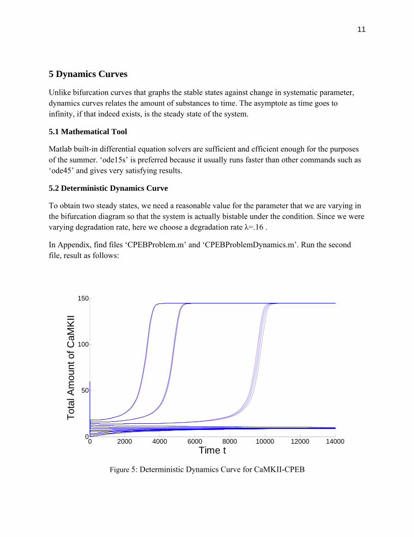
5 Dynamics Curves

Unlike bifurcation curves that graphs the stable states against change in systematic parameter, dynamics curves relates the amount of substances to time. The asymptote as time goes to infinity, if that indeed exists, is the steady state of the system.

5.1 Mathematical Tool

Matlab built-in differential equation solvers are sufficient and efficient enough for the purposes of the summer. ‘ode15s’ is preferred because it usually runs faster than other commands such as ‘ode45’ and gives very satisfying results.

5.2 Deterministic Dynamics Curve

To obtain two steady states, we need a reasonable value for the parameter that we are varying in the bifurcation diagram so that the system is actually bistable under the condition. Since we were varying degradation rate, here we choose a degradation rate λ=.16 .

In Appendix, find files ‘CPEBProblem.m’ and ‘CPEBProblemDynamics.m’. Run the second file, result as follows:

0 2000 4000 6000 8000 10000 12000 140000

50

100

150

Time t

Tot

al A

mou

nt o

f CaM

KII

Figure 5: Deterministic Dynamics Curve for CaMKII-CPEB

12

There are clearly two steady states in the system. The upper steady state is close to 150 and lower steady state is around 20. If we were to draw a line representing λ=.16 in figure 4, it will intersect the “S” curve at the exact same steady states. The dynamics curve and bifurcation curve should agree with each other. However, since we want to establish a comparison between the deterministic and stochastic approaches, figure 5 has a little too many curves. We want to decrease the number of curves so that we could compare curve to curve. Hence, run Appendix file ‘CPEBProblemDynamics2.m’ and obtain the following:

0 500 1000 1500 2000 2500 3000 3500 4000 4500 50000

50

100

150

Time t

Tot

al A

mou

nt o

f CaM

KII(

mol

)

Figure 6: Deterministic Dynamics Curve for CaMKII-CPEB with two initial conditions

5.3 Thoughts on Dynamics Curves

This is probably the simplest and most direct tool of all. In theory (and in my brief practice of this method), there should not be any problem at all. If the curves converge, then the system has according steady states. If it diverges, then the system does not have a steady state. It demonstrates the behaviors of the system in the most direct and simple way possible. If stability of a system is in doubt, it is a good idea to check the dynamics curves first, just to check upon the behavior of the system and make sure it is understood correctly.

13

6 Stochastic Approach

As mentioned in the beginning, deterministic approach is a bit far from the biological reality. Proteins that govern the translation machinery in the model are believed to exist in very low concentration. In this situation, reactions do not happen for sure. To model biology more closely, we implement stochasticity into the previous deterministic model via Gillespie algorithm.

6.1 Gillespie Algorithm

Figure 7: Gillespie Algorithm

14

6.2 Toy Problem for Gillespie Implementation

Though the following problem has higher dimensionality than CaMKII-CPEB problem, it is still simpler due to its monostable nature.

6.2.1 Elementary Kinetics

6.2.2 Differential Equations

)4()3()2()1()1(

521 xkxkxxkdt

dx

)11()3()2()1()2(

1121 xkxkxxkdt

dx

)4()9()3()3()2()1()3(

4321 xkxxkxkxxkdt

dx

)4()4()9()3()4(

543 xkxkxxkdt

dx

15

6.2.3 Deterministic Dynamics Curve

Find files ‘Game.m’ and ‘callGame.m’ in Appendix. Run ‘callGame.m’ to obtain the following:

0 50 100 150 200 250 300 350 400 450 5000

0.5

1

1.5

2

2.5

t

Con

cent

ratio

n

Figure 8: Deterministic Dynamics Curve for Toy Problem

)11()7()5()8()4()5(

9765 xkxxkxkxkdt

dx

)10()6()4()6(

105 xxkxkdt

dx

)8()7()5()8()7(

976 xkxxkxkdt

dx

)8()()7()5()8(

687 xkkxxkdt

dx

)8()4()9()3()9(

843 xkxkxxkdt

dx

)10()11()11()10(

10911 xkxkxkdt

dx

)11()11()10()6()11(

11910 xkxkxxkdt

dx

16

6.2.4 Stochastic Dynamics Curve

Find file ‘Gillepsie.m’ and ‘SampleGillespie.m’ in Appendix. Run ‘SampleGillespie.m’ and obtain the following (let s = 3000 in ‘Gillespie.m’):

0 500 1000 1500 2000 2500 300045

50

55

60

65

70

75

t

Con

cent

ratio

n

Figure 9: Stochastic Dynamics Curve for Toy Problem

6.2.5 Comparison between two approaches

**First note that time is not on the same scale between figures 8 and 9.

We notice that the curves in figures 8 and 9 have almost identical shapes. There is a dip in concentration in the beginning. Concentration climbs back to where it started, as time goes on. The difference, as expected, is that the stochastic curve is not as smooth as the deterministic one. The population change happens in discrete steps in the stochastic model. Thus, not surprisingly, we see a bumpy curve.

17

0 500 1000 1500 2000 2500 3000200

300

400

500

600

700

800

t

Con

cent

ratio

n

Figure 10: Stochastic Dynamics Curve for Toy Problem with higher concentration

If we start with an initial condition that is 10 times the one we worked with in figure 9, we get a less bumpy curve in figure 10. This curve looks even more like the deterministic curve. This is in fact what we suspect because after concentration of reactants increases over a certain threshold and becomes large enough, stochastic model should completely resemble that of deterministic approach.

18

6.3 Gillespie Implementation in CaMKII-CPEB Problem

Find ‘CPEBProblemStochasticDynamics.m’ in Appendix. Run it to obtain the stochastic curves of the CaMKII-CPEB model as follows:

Figure 11: Stochastic Dynamics Curve for CaMKII-CPEB Problem

6.4 Discussion on Stochastic Models and Gillespie Implementation

Unlike the deterministic models, with all initializing conditions the same, stochastic models give different results on each run and have different run time. Also, it typically takes longer to run a stochastic method than it does a deterministic one. This is mainly because in a stochastic model, random numbers are generated to assign time steps. Depending upon the results from random number generator, various reactions might happen and they happen according to various amount of time. Because it is also relatively expensive to generate a random number, the stochastic process that depends essentially on radon number generators is expensive to simulate and take very long time to run.

19

7 Discussion

We compare the results from two approaches – figures 6 and 11. The red curves have the same initial condition and the blue ones have the same initial condition. However, the curves behave quite differently in the two graphs. The red stochastic curve behaves somewhat as expected. Like its deterministic counterpart, we first see a dip, though not quit as deep as in the deterministic model, and then a climb. Because stochastic simulations are rather expensive to run, I set max runtime to 5000. However, if more efficient implementation is able to take the simulation in longer time frame, it is reasonable to believe that the red curve would eventually converge to its deterministic counterpart. The story is quite different with the blue curve. There is no sign of the stochastic blue curve going to the lower steady state at all. It is converging to an upper state even faster than the red curve. There could be many reasons why that happened. The most plausible two are: 1) Stochasticity destroys bistability and leaves us with a monostable system. 2) The systems in the stochastic simulations weren’t initialized correctly. Due to the time limitation of the REU program, there is not a chance to test just yet which one of the two is causing the discrepancy.

8 Acknowledgments

This work is partially funded by NSF REU Grant DMS-0755294. Special thanks dedicated to Dr. Harel Shouval, Dr. Naveed Aslam and Jeffrey Gavornik for their tremendous help and support throughout the summer.

9 References

1. Allgower, E.L., Georg, K. (1990). Numerical Continuation Methods: An Introduction. Springer-Verlag, New York.

2. Ullah, M., Schmidt, H., Cho, K.H. and Wolkenhauer, O. (2006). Deterministic modeling and stochastic simulation of biochemical pathways using MATLAB. IEE Proceedings-Systems Biology 153, 53-60.

20

Appendix

funccurve.m 21

testfunc.m 22

cont.m 22

curve.m 24

testcurve.m 26

CPEBProblem.m 26

CPEBProblemDynamics.m 27

CPEBProblemDynamics2.m 28

Game.m 28

callGame.m 29

SampleGillespie.m 29

Gillespie.m 30

CPEBProblemStochasticDynamics.m 31

21

funccurve.m

function out = curve%% Curve file of circle% out{1} = @curve_func; out{2} = @defaultprocessor; out{3} = @options; out{4} = [];%@jacobian; out{5} = [];%@hessians; out{6} = [];%@testf; out{7} = [];@userf; out{8} = [];@process; out{9} = [];@singmat; out{10} = [];@locate; out{11} = [];@init; out{12} = [];@done; out{13} = @adapt;%--------------------------------------------------------- function func = curve_func(arg) x = arg;

func = x(2)^5 - 15*x(2)^4 + 85*x(2)^3 - 225*x(2)^2 + 274*x(2) - x(1);

%---------------------------------------------------------function option= options option = contset; varargout{1} = option;%----------------------------------------------------------function varargout = defaultprocessor(varargin) if nargin > 2 s = varargin{3}; varargout{3} = s; end

% no special data varargout{2} = nan;

% all done succesfully varargout{1} = 0;%----------------------------------------------------------function [res,x,v] = adapt(x,v)res = []; % no re-evaluations needed

22

testfunc.m

disp('>> init;');init;

disp('>> [x,v,s]=cont(@curve,[1;0]);');[x,v,s]=cont(@funccurve,[1;0]);

plot(x(1,:),x(2,:))

cont.m

function [xout, vout, sout, hout, fout] = cont(varargin)%% CONTINUE(cds.curve, x0, v0, options)%% Continues the curve from x0 with optional directional vector v0% options is a option-vector created with CONTSET% The first two parameters are mandatory.

% WM: Rearranged many things throughout the code to put it% all in a more logical orderglobal sys cds driver_window MC% Interactive plottingstop;drawnow;if isfield(MC,'mainwindow') status = MC.mainwindow.mstatus; if isfield(MC.mainwindow,'options_window') plotpoints = get(MC.mainwindow.options_window,'Userdata'); else plotpoints = 1; endelse MC.D2 = [];MC.D3 = [];MC.numeric_fig = []; status = [];plotpoints = inf; MC.mainwindow.duration = []; MC.mainwindow.mstatus = [];endset(status,'String','computing');

if (nargin < 6)% case not extend cds = []; cds.curve = ''; warning off; lastwarn('');

23

% Parse given options [cds.curve, x0, v0, opt] = ParseCommandLine(varargin{:}); % Do some "stupid user" checks checkstupid(x0); cds.ndim = length(x0); curvehandles = feval(cds.curve); cds.curve_func = curvehandles{1}; cds.curve_defaultprocessor = curvehandles{2}; cds.curve_options = curvehandles{3}; cds.curve_jacobian = curvehandles{4}; cds.curve_hessians = curvehandles{5}; cds.curve_testf = curvehandles{6}; cds.curve_userf = curvehandles{7}; cds.curve_process = curvehandles{8}; cds.curve_singmat = curvehandles{9}; cds.curve_locate = curvehandles{10}; cds.curve_init = curvehandles{11}; cds.curve_done = curvehandles{12}; cds.curve_adapt = curvehandles{13}; % Read out all options or set default values % % Get options from curve file options = feval(cds.curve_options);% options = feval(cds.curve, 'options'); % Merge options from curve with cmdline, cmdline overrides curve cds.options = contmrg(opt, options); cds.options.MoorePenrose = contget(cds.options, 'MoorePenrose', 1); cds.options.SymDerivative = contget(cds.options, 'SymDerivative', 0); cds.options.SymDerivativeP = contget(cds.options, 'SymDerivativeP', 0); cds.options.Increment = contget(cds.options, 'Increment', 1e-5); cds.options.MaxNewtonIters = contget(cds.options, 'MaxNewtonIters', 3); cds.options.MaxCorrIters = contget(cds.options, 'MaxCorrIters', 10); cds.options.MaxTestIters = contget(cds.options, 'MaxTestIters', 10); cds.options.FunTolerance = contget(cds.options, 'FunTolerance', 1e-6); cds.options.VarTolerance = contget(cds.options, 'VarTolerance', 1e-6); cds.options.TestTolerance = contget(cds.options, 'TestTolerance', 1e-5); %%%%%%%%%%%%%%%%%%%%%%%%%%%%%%%%%%%%%%

Userfunctions = contget(cds.options, 'Userfunctions',0); %%%%%%%%%%%%%%%%%%%%%%%%%%%%%%%%%%%%%% Singularities = contget(cds.options, 'Singularities', 0); WorkSpace = contget(cds.options, 'WorkSpace', 0); Backward = contget(cds.options, 'Backward',0); CheckClosed = contget(cds.options, 'CheckClosed', 50); npoints = contget(cds.options, 'MaxNumPoints', 5000); Adapt = contget(cds.options, 'Adapt', 3); Locators = contget(cds.options, 'Locators', []);

24

IgnoreSings = contget(cds.options, 'IgnoreSingularity', []); %%%%%%%%%%%%%%%%%%%%%%%%%%%%%%%%%%%%% UserInfo = contget(cds.options, 'UserfunctionsInfo', []); %%%%%%%%%%%%%%%%%%%%%%%%%%%%%%%%%%%%% cds.h = contget(cds.options, 'InitStepsize' , 0.001); cds.h_max = contget(cds.options, 'MaxStepsize' , 0.06); cds.h_min = contget(cds.options, 'MinStepsize' , 1e-5); ** The rest of the code is unchanged. Should read the same as it was downloaded.**

curve.m

function out = curve%% Curve file of circle% out{1} = @curve_func; out{2} = @defaultprocessor; out{3} = @options; out{4} = [];%@jacobian; out{5} = [];%@hessians; out{6} = [];%@testf; out{7} = [];@userf; out{8} = [];@process; out{9} = [];@singmat; out{10} = [];@locate; out{11} = [];@init; out{12} = [];@done; out{13} = @adapt;%--------------------------------------------------------- function func = curve_func(arg) x = arg;

%lambda1 = 0.001;k1 = 0.08;k11 = 0.5;k2 = 0.08;k3 = 0.85;k33 = 0.01;k4 = 0.05;k5 = 0.016;k55 = 0.05;k6 = 0.002;k7 = 0.9;k77 = 0.075;

25

k8 = 0.022;k9 = 0.012;k99 = 0.001;k10 = 0.05;P = 0.0085;E = 6;yT = 100.0;BASAL = 0.3;

ddt1 = -k1*x(1)*x(2) + k11*x(4) + k4*x(5) + k10*x(8) - x(9)*(x(1)-BASAL);ddt2 = -k1*x(1)*x(2) - k3*x(2)*P - k5*(yT-x(3))*x(2) + 2*k2*x(4) + k11*x(4) + k33*x(5) + k55*x(6) +k6*x(6)- x(9)*(x(2)-BASAL);ddt3 = -k7*x(3)*P - k9*x(3)*E + k77*x(7) + k99*x(8) + k10*x(8) + k6*x(6);ddt4 = k1*x(1)*x(2) - k2*x(4) - k11*x(4);ddt5 = k3*x(2)*P - k33*x(5) - k4*x(5);ddt6 = k5*(yT-x(3))*x(2) - k55*x(6) - k6*x(6);ddt7 = k7*x(3)*P - k77*x(7) - k8*x(7);ddt8 = k9*x(3)*E - k99*x(8) - k10*x(8);

func = [ddt1;ddt2;ddt3;ddt4;ddt5;ddt6;ddt7;ddt8];

%---------------------------------------------------------function option= options option = contset; varargout{1} = option;%----------------------------------------------------------function varargout = defaultprocessor(varargin) if nargin > 2 s = varargin{3}; varargout{3} = s; end % no special data varargout{2} = nan;

% all done succesfully varargout{1} = 0;%---------------------------------------------------------- function [res,x,v] = adapt(x,v)res = []; % no re-evaluations needed

26

testcurve.m

disp('>> init;');init;

disp('>> [x,v,s]=cont(@curve,[3.3103;0.3417;10.8092;0.1560;0.0411;9.3773;0.8525;15.2601;.25]);');[x,v,s]=cont(@curve,[3.3103;0.3417;10.8092;0.1560;0.0411;9.3773;0.8525;15.2601;.25]);

m = x(1,:) + x(2,:) + 2*x(4,:);plot(x(9,:),m)

CPEBProblem.m

function dcdt = CPEBProblem(t,x)

lambda1 = 0.16;k1 = 0.08;k11 = 0.5;k2 = 0.08;k3 = 0.85;k33 = 0.01;k4 = 0.05;k5 = 0.016;k55 = 0.05;k6 = 0.002;k7 = 0.9;k77 = 0.075;k8 = 0.022;k9 = 0.012;k99 = 0.001;k10 = 0.05;P = 0.0085;E = 6;yT = 100.0;BASAL = 0.3;

ddt1 = -k1*x(1)*x(2) + k11*x(4) + k4*x(5) + k10*x(8) - lambda1*(x(1)-BASAL);

27

ddt2 = -k1*x(1)*x(2) - k3*x(2)*P - k5*(yT-x(3))*x(2) + 2*k2*x(4) + k11*x(4) + k33*x(5) + k55*x(6) +k6*x(6)- lambda1*(x(2)-BASAL);ddt3 = -k7*x(3)*P - k9*x(3)*E + k77*x(7) + k99*x(8) + k10*x(8) + k6*x(6);ddt4 = k1*x(1)*x(2) - k2*x(4) - k11*x(4);ddt5 = k3*x(2)*P - k33*x(5) - k4*x(5);ddt6 = k5*(yT-x(3))*x(2) - k55*x(6) - k6*x(6);ddt7 = k7*x(3)*P - k77*x(7) - k8*x(7);ddt8 = k9*x(3)*E - k99*x(8) - k10*x(8);

dcdt = [ddt1;ddt2;ddt3;ddt4;ddt5;ddt6;ddt7;ddt8];

CPEBProblemDynamics.m

clear allclc

tspan = [0 14000];

for i = 0:60:60 for j = 0:10:100 x0 = [i 0 j 0 0 0 0 0]; [t x] = ode15s('CPEBProblem', tspan, x0); y = x(:,1) + x(:,2) + 2*x(:,4); plot(t,y,'r') hold on endend

for j = 0:10:100 for i = 0:10:60 x0 = [i 0 j 0 0 0 0 0]; [t x] = ode15s('CPEBProblem', tspan, x0); y = x(:,1) + x(:,2) + 2*x(:,4); plot(t,y,'b') hold on endend

xlabel('Time t')ylabel('Total Amount of CaMKII')

28

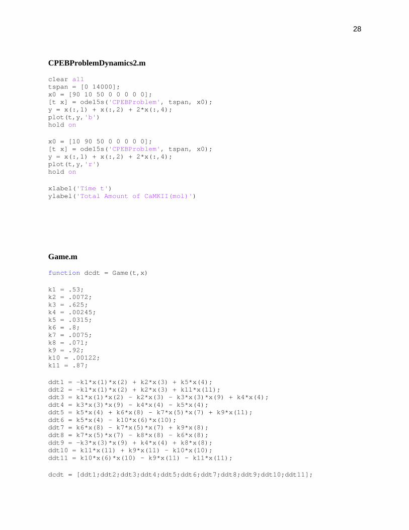
CPEBProblemDynamics2.m

clear alltspan = [0 14000];x0 = [90 10 50 0 0 0 0 0];[t x] = ode15s('CPEBProblem', tspan, x0);y = x(:,1) + x(:,2) + 2*x(:,4);plot(t,y,'b')hold on

x0 = [10 90 50 0 0 0 0 0];[t x] = ode15s('CPEBProblem', tspan, x0);y = x(:,1) + x(:,2) + 2*x(:,4);plot(t,y,'r')hold on

xlabel('Time t')ylabel('Total Amount of CaMKII(mol)')

Game.m

function dcdt = Game(t,x)

k1 = .53;k2 = .0072;k3 = .625;k4 = .00245;k5 = .0315;k6 = .8;k7 = .0075;k8 = .071;k9 = .92;k10 = .00122;k11 = .87;

ddt1 = -k1*x(1)*x(2) + k2*x(3) + k5*x(4);ddt2 = -k1*x(1)*x(2) + k2*x(3) + k11*x(11);ddt3 = k1*x(1)*x(2) - k2*x(3) - k3*x(3)*x(9) + k4*x(4);ddt4 = k3*x(3)*x(9) - k4*x(4) - k5*x(4);ddt5 = k5*x(4) + k6*x(8) - k7*x(5)*x(7) + k9*x(11);ddt6 = k5*x(4) - k10*x(6)*x(10);ddt7 = k6*x(8) - k7*x(5)*x(7) + k9*x(8);ddt8 = k7*x(5)*x(7) - k8*x(8) - k6*x(8);ddt9 = -k3*x(3)*x(9) + k4*x(4) + k8*x(8);ddt10 = k11*x(11) + k9*x(11) - k10*x(10);ddt11 = k10*x(6)*x(10) - k9*x(11) - k11*x(11);

dcdt = [ddt1;ddt2;ddt3;ddt4;ddt5;ddt6;ddt7;ddt8;ddt9;ddt10;ddt11];

29

callGame.m

clear all

x0 = [2.5 2.5 0 0 0 0 2.5 0 2.5 3 0]';

tspan=[0:.01:600];

[t,x] = ode15s('Game',tspan,x0);

plot(t,x(:,1));xlabel('t')ylabel('Concentration')

SampleGillespie.m

clear all

prob = [.0088 .0072 .01038 .00245 .0315 .8 .00012 .071 .92 .00002 .87]';

reaction = [-1 1 0 0 1 0 0 0 0 0 0; -1 1 0 0 0 0 0 0 0 0 1; 1 -1 -1 1 0 0 0 0 0 0 0; 0 0 1 -1 -1 0 0 0 0 0 0; 0 0 0 0 1 1 -1 0 1 0 0; 0 0 0 0 1 0 0 0 0 -1 0; 0 0 0 0 0 1 -1 1 0 0 0; 0 0 0 0 0 -1 1 -1 0 0 0; 0 0 -1 1 0 0 0 1 0 0 0; 0 0 0 0 0 0 0 0 1 -1 1; 0 0 0 0 0 0 0 0 -1 1 -1];

initial = [750 750 0 0 0 0 750 0 750 900 0]';

[x, t] = Gillespie(reaction, prob, initial);

plot(t,x(1,:));xlabel('t')ylabel('Concentration')

30

Gillespie.m

function [nn, tt] = Gillespie(M, P, I)format long n = I; %initial populationnn = [];t = 0; %initial timett = [];stop = 5000; %length of durationv = size(I,1);w = size(M,2);rand('state', sum(100*clock)); %reset random number generator

%time evolution on the outer loopwhile t <= stop tt = [tt t]; %record time m = n; %copy the last population state nn = [nn n]; %record population

%randomly choose the chemical, 'c1' c1 = floor(1.5 + (v-1)*rand(1)); %find the reactions that 'c1' is involved in rr = []; pp = []; for i = 1:1:w if M(c1,i) ~= 0 rr = [rr M(:,i)]; pp = [pp P(i)]; end end %calculate propensity vector 'p' [row, column] = size(rr); p = []; sp = []; for i = 1:1:column mm = pp(i); for j = 1:1:row if rr(j,i) == -1 mm = mm*m(j,1); end end p = [p mm]; astr = sum(p); %cumulative propensity sp = [sp sum(p)]; end %randomly choose the reaction, 'r' if astr <= 0 t = t; else c3 = rand(1); c2 = c3*astr;

31

r = 1; while c2 > sp(r) r = r + 1; end %reaction changes population n = rr(:,r) + n; %calculate time till next reaction tau = -1/astr*log(rand(1)); tau = tau/10; t = t + tau; end end tt = [tt t];nn = [nn n];

CPEBProblemStochasticDynamics.m

clear allformat long eprob = [.00002656 .5 .08 .00028225 .01 .05 .00000531 .05 .002 .00029885 .075 .022 .00000398 .001 .05 .16 .16]'; reaction = [-1 1 0 0 0 1 0 0 1 0 0 0 0 0 1 -1 0; -1 1 2 -1 1 0 -1 1 0 0 0 0 0 0 0 0 -1; 0 0 0 0 0 0 0 0 1 -1 1 0 -1 1 1 0 0; 0 0 0 0 0 0 -1 1 0 0 0 1 0 0 0 0 0; 1 -1 -1 0 0 0 0 0 0 0 0 0 0 0 0 0 0; 0 0 0 1 -1 -1 0 0 0 0 0 0 0 0 0 0 0; 0 0 0 0 0 0 1 -1 -1 0 0 0 0 0 0 0 0; 0 0 0 0 0 0 0 0 0 1 -1 -1 0 0 0 0 0; 0 0 0 0 0 0 0 0 0 0 0 0 1 -1 -1 0 0; 0 0 0 -1 1 1 0 0 0 -1 1 1 0 0 0 0 0; 0 0 0 0 0 0 0 0 0 0 0 0 -1 1 1 0 0]; initial = [300 2700 1500 1500 0 0 0 0 0 0 18]';[x, t] = Gillespie(reaction, prob, initial);y = x(1,:) + x(2,:) + 2*x(5,:);plot(t,y,'r')hold on

initial = [2700 300 1500 1500 0 0 0 0 0 0 18]';[x, t] = Gillespie(reaction, prob, initial);y = x(1,:) + x(2,:) + 2*x(5,:);plot(t,y,'b')hold on