Cyclone Database Manager

A tool for converting point data from cyclone observations into tracks and wind speed profiles in a GIS.

FREDERIC MOUTON OLA NORDBECK

A PreView-Project for The Early Warning Unit United Nations Environment Program

Global Resource Information Database - Geneva (UNEP/DEWA/GRID-Geneva)

Département de Géographie

Université de Genève Directeur de mémoire: Pascal Peduzzi

1

Abstract A comprehensive investigation was carried out to identify the regions affected by different cyclone events. The observations of historical cyclone events are sparse globally, which forced this investigation to estimate the radial wind speed profile by using a parametric model. The selected model was created by G.J. Holland 1980 (Bureau of Meteorology, Australia) and is considered to be generally superior to other similar models by a wide range of tropical cyclone specialists. This model was programmed for calculating winds speed regions around cyclone tracks for different wind speed strengths. Another essential part of the program is to structure the wide range of gathered data sets from different sources. This program can be an important tool for building a unified global cyclone database, including first level basic meteorological information (the geographical position and date of the cyclone observation, the measured wind speed and the central pressure) and geospatial data (the cyclone tracks, and their radial wind speed profiles). This global cyclone database renders possible post-analysis of historical cyclone events. Keywords: cyclone, geospatial data, parametric model, wind speed, wind speed profile, wind speed buffer.

2

Acknowledgments

We are grateful for the assistance from the following persons without their help this work

wouldn’t be realized:

Nanette Lomarda WMO (World Meteorological Organisation)

for the contacts and documentation on cyclones

We are also grateful for the following specialists’ advices on cyclone modelling:

Greg Holland, Bruce Harper Bureau of Meteorology, Australia

Mark D. Powell The National Oceanic and Atmospheric Administration (NOAA), USA

Chip Guard, Sim Aberson,Chris Landsea

NOAA, USA Kerry A. Emanuel

Department of Earth, Atmospheric, and Planetary Sciences, MIT, USA Leslie.Weiner-Leandro

Federal Emergency Management Agency (FEMA), USA

We also bow gratefully for our close colleagues at GRID-Geneva for sharing their technical knowledge and warm accomodation:

Andrea De Bono, Hy Dao, Christian Herold, Pascal Peduzzi, Stefan Schwarzer, Ron Witt

Last but not least, we would like to thank Charles Hussy for sharing his enthousiasm of Geomatics

3

1 INTRODUCTION 4

2 EXAMPLES OF EXISTING WIND SPEED BUFFERS 5

2.1 THE OUTER CLOSED ISOBAR AS A WIND SPEED BUFFER LIMIT 5 2.2 THE CATS (THE CONSEQUENCE ASSESSMENT TOOL SET) 6

3 POINT ESTIMATION OF TRANSVERSAL BUFFERS 9

3.1 GREG HOLLAND’S PARAMETRIC MODEL 9 3.2 APPLICATION OF GREG HOLLAND’S MODEL 10 3.3 SYMMETRIC BUFFER 13 3.4 ASYMMETRIC BUFFER 14 3.5 DISCUSSION AND REFINEMENTS ON THE CHOICE OF PARAMETERS 23

4 FROM POINT ESTIMATION TO GLOBAL BUFFERS 24

4.1 SYMMETRIC CASE 24 4.2 ASYMMETRIC CASE 25

5 AUTOMATION OF THE MODEL 27

6 CONCLUSION 29

6.1 CURRENT AND FUTURE APPLICATIONS 29 6.2 FURTHER DEVELOPMENTS 30

7 REFERENCES 31

APPENDIX A. CycloneDatabaseManager manual APPENDIX B. Visual Basic code APPENDIX C. Saffir-Simpson scale APPENDIX D. Comparison of the modelled Gwenda and the measured wind speed

buffers of the Bureau of Meteorology in Australia

4

1 INTRODUCTION

Background This work started as a study of the possibilities to identify the regions affected by different cyclone events, "windspeed buffers". This investigation was carried out, by GRID-Geneva, in order to extract the number of persons affected by unique cyclone events globally. Since this post-cyclone analysis by GRID-Geneva was carried out on a global scale the wind speed buffer estimations had to be adequate to the severe cyclone events worldwide.

Aim The aim of this study is to build a tool for unifying the severe historic global cyclone data and to identify the regions affected by the different cyclone events. The main purpose of this tool is to facilitate the composition of a global cyclone data base, including first level basic meteorological information (the geographical position and date of the cyclone observation, the measured wind speed and the central pressure) and geospatial data (the cyclone tracks, and their wind buffers).

Method In order to fulfil the main aim of this research it was important to identify and verify existing projects. This research didn’t allow us to identify any relevant study for our purposes, that is to say any earlier work that is possible to apply on a global scale at a low cost. Another important detail was that our research comprised historical cyclone events, as the purpose of our work was to establish a tool for facilitating the creation of a cyclone database for post-cyclone analysis. This implies limited data accessibility, since the observations already are carried out and the quantity and quality of the data variables are therefore difficult to ameliorate. The sparse observations of historic cyclone events forced us therefore to estimate the radial wind speed profile, wind speed buffer, by using a parametric model. By a fruitful collaboration with Nanette Lomarda, Scientific Officer at World Meteorological Organisation (WMO) we were able to get in contact with a wide range of tropical cyclone specialists, who all referred to the same parametric model. A model created by Greg Holland at Bureau of Meteorology Australia (Holland, 1980), for calculating the wind and pressure profiles of a cyclone, in order to define its wind speed buffer. For a more detailed description of the data process see appendix A.

5

2 EXAMPLES OF EXISTING WIND SPEED BUFFERS A precise wind analyse of the outer circulation of tropical cyclones is difficult to construct and interpret. The ultimate solution would be frequently observations from different sources as islands, ships, coastal regions, aircraft, etc. but the observations of the outer circulation of tropical cyclones are generally quite sparse, and from different sources and are subject to substantial errors. These two reasons make it difficult to find accurate examples of cyclones horizontal wind structure on a global scale (Holland, G. J., 1997)

2.1 The outer closed isobar as a wind speed buffer limit The Radius of Outer Closed Isobar (ROCI) is one way of analysing and forecasting the outer circulation of tropical cyclones and it can be seen as an approach to identify a wind speed buffer. Identification of the outer closed isobar is only possible with the information of the cyclone structure and the structure change over time. Since the outer circulation probably is the easiest element to observe directly and the most difficult to infer remotely from satellite imagery, a homogeneous interpretation on a global level is hard to achieve. An extensive study of the outer circulation of tropical cyclones by the ROCI method would therefore be complicated and time consuming (Merrill, 2000).

Figure 1: The circle is the radius of the average outer closed isobar (Merrill, 2000)

6

A solution to this could be to identify an average radius of the outer closed isobar for different tropical cyclones within the different regions. This was done in Merrill (1984), where he identified the average size of twelve Atlantic cyclones by calculating the average radius of the outer closed isobar. He used also the average in intensity of the cyclones for identifying a cyclone’s change in shape over time. He divided thereafter the cyclone’s lifetime into four different phases: formative, immature, mature and decaying and determined the four phases with surrounding circles (see Figure 1, (Merrill 2000). These four circles can be seen as wind speed buffers since the average wind speed and pressure are given inside the circles. The work by Merrill is not possible to find for other cyclone basins and the circle size of the four lifetime phases for the twelve cyclones are not adequate for a study on global scale with different years represented.

2.2 The Cats (the Consequence Assessment Tool Set) Another example of wind speed buffers is The Cats (the Consequence Assessment Tool Set) model, which is a GIS-based model, made for estimating losses after a cyclone or tropical storm. The CATS system estimates in real-time the population and civil resources at risk from threatening hurricanes and associated storm surge; its primary application is to assist preparation and recovery efforts in emergency planning, readiness actions, and the prepositioning of relief supplies and personnel. The module automatically parses advisory messages to extract current and forecast hurricane characteristics. Messages are usually disseminated every six hours, and contain observation and forecast data provided by the National Hurricane Center (NHC) in Miami, FL, the Central Pacific Hurricane Center (CPHC) in Honolulu, HI, or the Joint Typhoon Warning Center (JTWC) in Guam. The National Weather Service’s Family of Services, the NOAA Weather Wire, University Internet servers, or commercial vendors of meteorological data provide access to these messages. Hurricane data collected from the messages includes the current and forecast positions of the storm, its maximum wind speed, and the spatial distribution of winds around the storm centre. At each quadrant of the storm, and for its current and forecast positions, radial profiles of dynamic pressure and wind speed are analysed. Colour-coded damage bands are then generated which display results of structural response modelling, which correlates hurricane wind gust velocity and dynamic pressure to damage to various structure types. Figure 2 presents estimates of wind damage to mobile homes calculated by CATS for Hurricane Fran (September 1996). The light purple area represents light damage, yellow moderate damage, and red severe damage (http://www.saic.com, 1999)

7

Figure 2: Damage estimation of Fran (1996) with CATS (www.saic.com, 1999)

Since this application is made for estimations in real-time and the aim is uniquely predictive, the wind speed around the cyclone track is not identified. For a spatial analysis (the movement of cyclones, best cyclone tracks, and their radial wind speed profiles) and global post-analysis of storms, an estimation of the wind speed is important due to regions varying sensitivity (see figure below and Appendix C for Saffir-Simpson). A more precise description of the CATS is difficult to obtain since it is a commercial product (http://www.saic.com, 1999). CATS is today used by some important institutions, one example is FEMA's (Federal Emergency Management Agency) Mapping and Analysis Center, who use this model for estimating the losses after a hurricane or tropical storm (Personal contact with Leslie Weiner-Leandro at FEMA, July 2001). For more precise data FEMA has developed and are about to develop a program with different wind data to enable a more precise spatial analysis (the movement of cyclones, best cyclone tracks, and their radial wind speed profiles). This program is called U.S. HAZUS model and is expected to be available in 2003, according to Mark Powell at NOAA, the National Oceanic and Atmospheric Administration (Personal contact, July 2001).

8

Figure 3: Saffir Simpson Scale

Saffir-Simpson Scale The Saffir-Simpson Scale is used to classify the intensity of tropical storms and hurricanes. Category Pressure (millibars) Winds (knots) Winds (mpd) Surge (feet)Tropical Depression -- less than 34 less than 39 -- Tropical Storm -- 34-63 39-73 -- Category 1 Hurricane more than 980 64-82 74-95 4-5 Category 2 Hurricane 965-980 83-95 96-110 6-8 Category 3 Hurricane 945-965 96-113 111-130 9-12 Category 4 Hurricane 920-945 114-135 131-155 13-18

Category 5 Hurricane less than 920 more than 135 more than 155

more than 18

9

3 POINT ESTIMATION OF TRANSVERSAL BUFFERS In order to estimate wind speed buffers along the whole track, the first step is to estimate the wind speed profile at a certain time (corresponding to a certain position of the cyclone’s eye). As well as deduce the transversal buffers, i.e. right and left intervals on the line perpendicular to the track (and going through the cyclone’s eye) where the wind intensity is (or have been or will be) greater than a chosen wind speed threshold critV . For this purpose we built a wind speed profile model based on the known observed parameters.

3.1 Greg Holland’s parametric model The parametric model described in this chapter is defined by Greg Holland at the Bureau of Meteorology in Melbourne, Australia (Holland G.J., 1980) based on an original approach by Schloemer (ref, 1954). The model includes a formula for the wind speed at a given radius, i.e. the distance from a current point to the eye of the cyclone. For this model it is supposed that the cyclone is over the ocean, that the eye of the cyclone is stationary and that the surrounding winds follow a three-dimensional symmetry around a vertical axis (axisymmetric winds). It assumes that the tropical cyclone surface wind field follows:

Equation 1: Wind calculation (Holland G.J., 1980)

( )24

)(22

maxmax RffRePP

RRbRV

b

RR

centreenv

b

h −+⋅−⋅⎟⎠⎞

⎜⎝⎛⋅=

⎟⎠⎞

⎜⎝⎛−

ρ

Where: )(RVh : Gradient wind speed at distance R from the eye (in m/s)

b : Parameter that changes the shape of the radial profile centreP : Central pressure (in Pa)

envP : The asymptotic environmental pressure (in Pa)

maxR : The radius of maximum winds (in meters) as can be seen on the curve below R : The radius where wind speed is )(RVh (in meters) ρ : The air density, assumed constant =1.15 kg m⎯³ f : The Coriolis parameter =2*(Earth's angular velocity)*sin(latitude) where the Earth angular

velocity equals 0.0000729 radians/s. This formula gives a wind speed profile whose shape can be seen on Figure 4 (for parameters: b =1.5, envP =1015 hPa, centreP =990 hPa, maxR =10000 m, latitude =45°):

10

Figure 4: Wind speed profile for Greg Holland’s stationary model

3.2 Application of Greg Holland’s model The parameters mentioned in the introduction and in the formula above are necessary for a functioning model. An important part of the work was therefore to find the cyclone data for the cyclone basins worldwide. With the following data: the successive positions of cyclone’s eye, corresponding central pressure and maximum observed wind speed. This new structure of the different important meteorological parameters enabled spatial analyses, as for instance the movement of cyclones (tracks) and their radial wind speed profiles. The parameters concerning the geographical position and the intensity of the tropical cyclone are not sufficient for applying Greg Holland’s model. To allow computation of the wind speed around a cyclone track, i.e. to estimate a zone around the cyclone corresponding to a wind speed above a certain fixed threshold, some variables have to be identified. There is a need to: • Chose a value for parameter b , which dictates the shape of the pressure or wind speed

profile. • Determine the asymptotic environmental pressure envP • Estimate the radius of maximum wind speed maxR • Take into account the fact that the cyclone is not stationary

)(RVh

maxR )(mR

)( 1−msV

11

The b parameter, the shape of the pressure or wind speed profile That parameter changes the shape of the profile as can be seen on Figure 5, where, for same other parameters as above ( envP =1015 hPa, centreP =990 hPa, maxR =10000 m, latitude =45°), the three values b =1, b =1.5 and b =2.5 are chosen:

Figure 5: Effect of b parameter on the wind speed profile shape

A first approach consists in choosing a constant value for the b parameter. Physical constricts ensure that 1<b <2.5, supported by a climatological discussion, and for establishing wind speed buffers it is appropriate to use a low value since a high value gives wind speed buffers with too short intervals (Holland G.J., 1980). Following Greg Holland’s recommendation a value of 1.5 was used although Bruce Harper was suggesting a value of 1 (Personal contact with Holland G.J. and Harper Bruce, July 2001). By using b = 1 the profile would also be constrained to a single profile, as the profile of Schloemer’s relation, which markedly underestimates the maximum winds and overestimates the radial extent of destructive winds (see Figure 5 above). A second approach for estimating parameter b using Greg Holland’s formula and using measurements of maximum wind speed will be described later.

b=1

b=2.5b=1.5

)(mR

)( 1−msV

12

The envP parameter, the asymptotic pressure The asymptotic pressure varies for the different cyclone events and the observations are primarily focused on the tropical eye’s central pressure. It is therefore difficult to obtain data about this parameter for the different cyclone events and an important simplification of this parameter is therefore inevitable. By defining climatic constants for the regions of the different cyclone basins this parameter can be seen as more adequate than by using an overall reference. These constants were defined with the help of Bruce Harper and Greg Holland and according to the authors it is possible to differentiate the regions as follows (Personal contact with Holland G.J. and Harper Bruce, July 2001): 1015 hPa in the North Atlantic, 1005 hPa in the NW Pacific and Australian region, 1008 hPa in the North and South Indian Ocean, 1010 hPa in the NE Pacific. The value of the NE Pacific is based on the proposed overall reference of the two above mentioned authors even though the standard atmospheric pressure is 1013 hPa.

The maxR parameter, the radius of maximum winds The maxR parameter is theoretically independent of the relative values of ambient and central pressure and also of the b parameter. It could therefore not be determined by the cyclone intensity data or by the shape of its profile. However, to be able to model the extension of the destructive winds within a cyclone without the information about the cyclone’s structure, the available data about the intensity has to be used. In order to estimate the maxR of a cyclone, Mark Powell at NOAA (Personal contact, July 2001) suggested to stratify the cyclones into three different classes related to the central pressure: Small, medium and large. Remark that the pressure field can be missing for some observations, and in those cases, Greg Holland’s model can not be used. The three classes were defined by aggregating the Saffir-Simpson scale (see appendix C), for the central pressure. By studying earlier cyclone events and their maxR , we were able to identify three likely distances for the maxR . Details, refinements and comments on that classification will be described later.

The movement of the cyclone’s eye The translation movement of the cyclone is not taken into account in the model. A rough but simple way to include this translation movement is to add the eye’s speed value to the speed given by the model (Personal contact with Holland G.J., July 2001), which results in a wind speed profile with a symmetric structure. This structure of a cyclone with double wind maxima, on both sides of the cyclone track, occurs under specific circumstances but it is exceptional. The symmetric way of illustrating a cyclone facilitates the modelling work, but the cyclone’s asymmetric characteristic is not to be neglected. The cyclone’s asymmetry can be obtained by calculating vectors i.e. by adding the translational vector to the windfield. This gives a net flow behind the cyclone, outflow ahead and a maximum wind speed on the cyclone’s right hand side in the Northern Hemisphere and on the left side in the Southern Hemisphere. In practice the eye’s speed intensity and direction can be estimated by using the time consecutive positions of the eye.

13

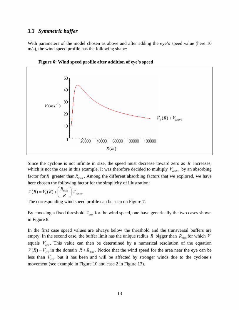
3.3 Symmetric buffer With parameters of the model chosen as above and after adding the eye’s speed value (here 10 m/s), the wind speed profile has the following shape:

Figure 6: Wind speed profile after addition of eye’s speed

Since the cyclone is not infinite in size, the speed must decrease toward zero as R increases, which is not the case in this example. It was therefore decided to multiply centreV by an absorbing factor for R greater than maxR . Among the different absorbing factors that we explored, we have here chosen the following factor for the simplicity of illustration:

centreh VR

RRVRV ⋅⎟⎠⎞

⎜⎝⎛+= max)()(

The corresponding wind speed profile can be seen on Figure 7. By choosing a fixed threshold critV for the wind speed, one have generically the two cases shown in Figure 8. In the first case speed values are always below the threshold and the transversal buffers are empty. In the second case, the buffer limit has the unique radius R bigger than maxR for which V equals critV . This value can then be determined by a numerical resolution of the equation

critVRV =)( in the domain R > maxR . Notice that the wind speed for the area near the eye can be less than critV but it has been and will be affected by stronger winds due to the cyclone’s movement (see example in Figure 10 and case 2 in Figure 13).

centreh VRV +)(

)( 1−msV

)(mR

14

Figure 7: Wind speed profile with absorbing term

Figure 8: Two cases for threshold

3.4 Asymmetric buffer The wind field in tropical cyclones is rarely, if ever, symmetric. Asymmetries arise from a range of processes, including: cyclone movement; location and structure of the cloudy and clear regions around the cyclone, including the spiral cloud bands; external influences from surrounding weather systems; and occasional high intensity transients, such as meso vortices. Further, transient conditions occur in which two maximum wind belts develop, with the outer contacting inwards and destroying the inner one (Holland G.J., 1997). The only processes routinely included in current parametric wind models are those arising from the cyclone movement.

)(mR

)(RVh

centreh VRV +)(

centreh VR

RRV ⋅⎟⎠⎞

⎜⎝⎛+ max)(

critV

)( 1−msV

critV

)(mR

)( 1−msV

15

As mentioned before; the simplest way to include in the model the asymmetry due to the movement, i.e. add the eye’s speed vector (translation) to the stationary model’s wind vector field (rotation). The cyclones in the Northern Hemisphere rotate anticlockwise (clockwise in the Southern Hemisphere) and the examples treated in this text are in north and the anticlockwise rotation will therefore be described. On the right-hand side of the cyclone’s track, the translation vector and the rotation vector are in the same direction, i.e. the two speed values are to be added. On the left-hand side, they move in opposite directions and the two speed values are to be subtracted. More generally, those two vectors make an angle as can be seen on the following figure in polar coordinates, where the wind speed is considered at a point M of radius R and angle θ , respectively at a point M’ of radius R′ and angle ψ .

Figure 9: Angle between rotation wind speed and eye’s translation speed

θ ′ M

centreVr

centreVr

uV

R

),( ϑRVh

r

ψR′

),( ψRVh ′r

centreVr

Vr

Vr

ϑ

Cyclone’s eye

Direction of cyclone’s centre

M’

16

The stationary model’s vector field is ϑϑ uRVRV hhrr⋅= )(),(

Where θur is the unitary vector perpendicular to the ray OM and pointing like the rotation direction (i.e. anticlockwise). Finally, wind speed is modelled by

centrehcentreh VuRVVRVRVrrrrr

+⋅=+= ϑϑϑ )(),(),(

whose norm is

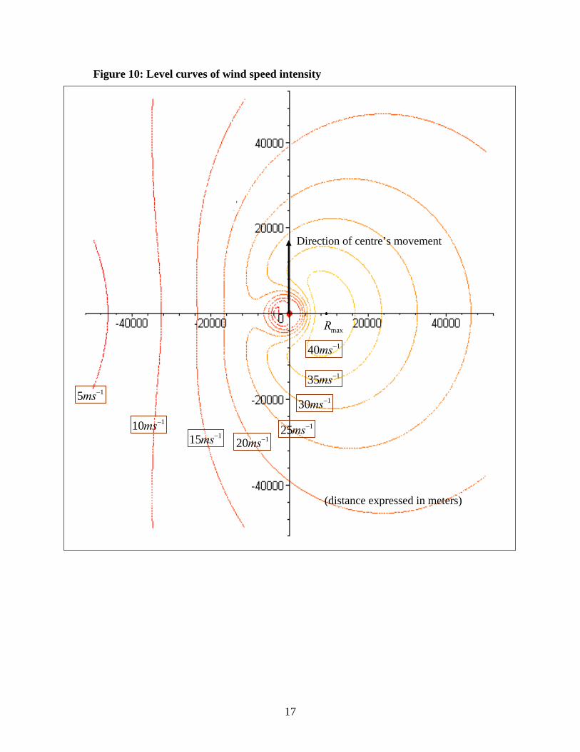
Level curves of ),( θRV have thereafter the following shape (Figure 10, with the same parameters as above). A 3-D picture of the graph of ),( θRV is presented in Figure 11 and the speed vector field can be seen in Figure 12.

)cos()(2)(),(),( 22 ϑϑϑ centrehcentreh VRVVRVRVRV ++==r

17

Figure 10: Level curves of wind speed intensity

maxR

Direction of centre’s movement

(distance expressed in meters)

140 −ms

135 −ms130 −ms

125 −ms120 −ms

110 −ms115 −ms

15 −ms

18

Figure 11: Graph of ),( θRV

)( 1−msV

Direction of centre’s movement

(distances are expressed in meters)

)( 1−msV

19

Figure 12: Speed vector field

maxR

(distance expressed in meters)

Direction of centre’s movement

20

For a given threshold critV , the region V > critV can have the following shapes, which lead to transversal buffer limits 1R and 2R as indicated in case 1, 2 and 3 below (Figure 13). Notice that some of the points between 1R and 2R are not actually moving with a speed greater than critV but they have or will do due to the cyclone’s movement.

Figure 13: Different cases for critical region

Case 2

Case 3

1R

2R1R

1R 2R2R

Case 1 (Empty buffer) 1R 2R

21

Limit 2R in the previous section is calculated, as a symmetric buffer but 1R needs to be computed or at least approximated as an asymmetric buffer.

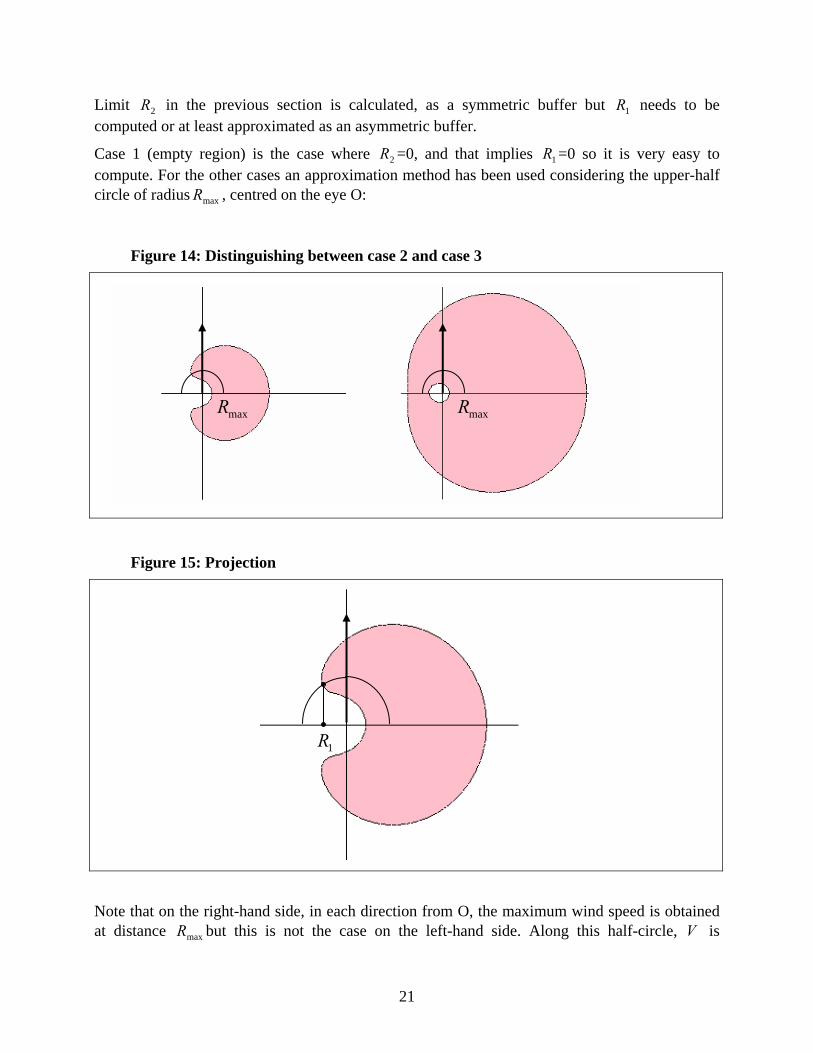
Case 1 (empty region) is the case where 2R =0, and that implies 1R =0 so it is very easy to compute. For the other cases an approximation method has been used considering the upper-half circle of radius maxR , centred on the eye O:

Figure 14: Distinguishing between case 2 and case 3

Figure 15: Projection

Note that on the right-hand side, in each direction from O, the maximum wind speed is obtained at distance maxR but this is not the case on the left-hand side. Along this half-circle, V is

maxR maxR

1R

22

decreasing from right to left. The case where V don’t decreases below critV along the half-circle is defined in case 3 and 1R is in this case computed by a method analogous to the one for 2R . In the case where V decreases below critV , 1R is approximated by using the projection of the point where V = critV as in the Figure 15.

Notice that the projection point determining 1R can be either on the right hand side or on the left side with respect to the origin (cyclone’s centre). To take into account these two different cases, the following convention was used: radius 1R will be positive if the projection is on the left (in the northern hemisphere) and negative if the projection is on the right side, i.e. if the two points for 1R and 2R are on the same side. In this case an elementary computation gives then the value of 1R :

⎟⎟⎠

⎞⎜⎜⎝

⎛

⋅⋅−−

−=centreh

centrehcrit

VRVVRVV

RR)(2)(

max

22max

2

max1

This leads to the following algorithm:

If Vcrit > (Vh(Rmax) + Vcentre) Then

‘Case 1:

R1 = R2 = 0

Else

‘Same as symmetric buffer for R2:

R2 = SOLVE(Vh(R) + (Rmax/R)*Vcentre – Vcrit = 0; R; R>=Rmax)

‘Distinguishing between case 2 and 3 for R1:

If Vcrit < (Vh(Rmax) – Vcentre) Then

‘Case 3

R1 = SOLVE(Vh(R) – (Rmax/R)*Vcentre – Vcrit = 0; R; R>=Rmax)

Else

‘Case 2

R1 = – Rmax*((Vcrit^2 – Vh(Rmax)^2 – Vcentre^2) / (2Vh(Rmax)Vcentre))

End If

End If

Several numerical resolutions were first proceeded using Microsoft Excel Solver, but were later changed for a simple dichotomy algorithm (see Visual Basic code appendix B) implemented in Microsoft Visual Basic. That for several reasons: it allows cross-verifications with earlier results; one has a better control when problems occur in particular cases, and our further objective is a minimum use (none if possible) of Microsoft Excel for best efficiency and transparencies.

23

3.5 Discussion and refinements on the choice of parameters

Estimation of parameter b The problem with choosing a constant value for the parameter b is the theoretical maximum wind speed intensity that depends almost uniquely upon the pressure value. It results sometimes in a great difference between the theoretical maximum values and the observed maximum speed intensities. As the maximum theoretical values are obtained at distance maxR , it is a simple computation to chose b such that the maximum theoretical value for stationary model equals the maximum relative (with respect to the centre) speed intensity:

( ) ( )centreenv

centreobscentreobs

ppfRVVVVe

b−

⋅+−⋅−⋅⋅= maxmaxmaxρ

As the Coriolis term is negligible and also because of the uncertainty in the determination of maxR , an approximation was made:

( )centreenv

centreobs

ppVVe

b−

−⋅⋅=

2maxρ

However, if the b value is not between 1 and 2.5, it’s important to consider the problem of physical coherence because b should be in that interval for physical and climatological reasons, as mentioned before e.g. too small values of b results in overestimated buffers. Further, the observed maximum wind speed are less reliable than the pressure observations since the metadata explaining the methodology of measurement and interpolations is insufficient. For those reasons, we have decided that if the computation gives a b -value less than one, it will be fixed at 1 and the same for values greater than 2.5, which are fixed at 2.5.

Estimation of maxR The uncertainty is important concerning the estimation of maxR . There’s no value for maxR in the observed data and as described before, the only possibillity to identify this value is to estimate

maxR using the pressure classes. The first approach was to define three pressure classes by aggregating classes in the Saffir-Simpson scale: p>980, 980>p>965, 965>p. These classes were thereafter used to define relevant maxR values based on examples of cyclone events with observed

maxR . However, choosing a fixed value of maxR for each of the three pressure classes leads to distinct differences between the classes and a piecewise linear function was therefore used between the determined classes. Further improvement of a maxR estimation could be done by dividing the cyclone’s life cycle into three phases: growing, mature and declining. For these different phases the link between central pressure and maxR is different and a great improvement of the buffer estimation could be achived if reasonable estimations of maxR was furnished by the providers.

24

4 FROM POINT ESTIMATION TO GLOBAL BUFFERS Construction of global buffers, wind speed buffer along the cyclone track, from transversal buffer values implies two main problems. Firstly, the width of a buffer along an entire track is not constant and such a buffer is rarely handled by a GIS-software; secondly, in the asymmetric case, left and right widths are not the same. The solution to the first problem may rely on dividing the track into smaller parts (interpolation) and to adjusting on each part a classical fixed-width buffer, this can easily be handled by a GIS-software. The solution to the second problem is more complicated and a totally different method was selected.

4.1 Symmetric case

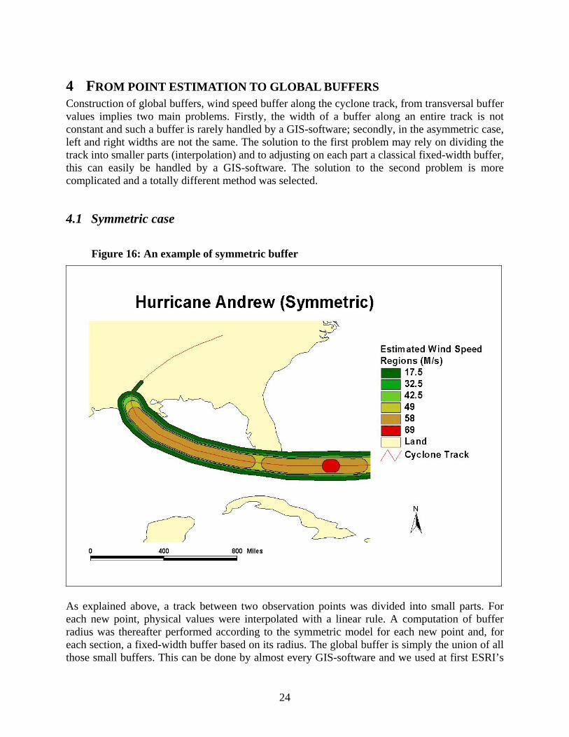
Figure 16: An example of symmetric buffer

As explained above, a track between two observation points was divided into small parts. For each new point, physical values were interpolated with a linear rule. A computation of buffer radius was thereafter performed according to the symmetric model for each new point and, for each section, a fixed-width buffer based on its radius. The global buffer is simply the union of all those small buffers. This can be done by almost every GIS-software and we used at first ESRI’s

25

ArcView. But the second time, the need of automation for treating a great number of cyclones simultaneously lead to program routines in ESRI’s ArcInfo. This work was carried out by Christian Herold at UNEP/GRID-Geneva. An example that was constructed in ArcView can be seen on Figure 16.

4.2 Asymmetric case In order to treat the asymmetry (and also varying width) in a simple way, it was decided to construct global buffer as polygons. For that purpose, it has first been computed on each measure point N an estimation of cyclone eye’s speed intensity and a perpendicular to cyclone eye’s speed direction using the two consecutive last point M and next point P as seen on Figure 17. The perpendicular taken is the bisectrix of angle (MNP).

Figure 17: Construction of transversal buffer points

Two points were computed, LargeBufferPoint and SmallBufferPoint on the perpendicular corresponding to the two previously computed radii 1R and 2R . All the points were handled by their longitude and latitude coordinates and all computations were made taking into account the sphericity of the earth surface. All corresponding functions are regrouped in a Visual Basic module named SphericGeom (See Appendix B). Once a LargeBufferPoint and a SmallBufferPoint were computed for each initial track point, it becomes easy in every GIS-software to construct the global buffer as a polygon. However,

M

N

P

R1

R2SmallBufferPoint

LargeBufferPoint

rVcentre

26

automation of that process for a large number of cyclones requires routines and has been done by Christian Herold at UNEP/GRID-Geneva using ArcInfo. An example can be seen on Figure 18.

Figure 18: An example of asymmetric buffer

27

5 AUTOMATION OF THE MODEL The observations of tropical cyclones worldwide are carried out by the different Regional Specialised Meteorological Centres (RSMCs) together with six Tropical Cyclone Warning Centres (TCWCs) of World Meteorological Organisation. The different observation centres are well coordinated and they keep the first level basic meteorological information (chronological data about the geographic localisation of the cyclones and their intensity) updated on all the global tropical cyclones events. This collaboration gives a broad range of global cyclone data, but the range of reported data imply problems due to differences in data structure. The following providers were found appropriate for covering the cyclone basins worldwide:

Organisations URL address

Unisys Weather: Http://weather.unisys.com/hurricane/

Typhoon 2000: Http://www.typhoon2000.ph/

Australian Severe Weather: Http://australiasevereweather.com/cyclone/

Atlantic Hurricane Track Maps & Images: Http://fermi.jhuapl.edu/hurr/index.html

Hawaii Solar Astronomy: Http://www.solar.ifa.hawaii.edu/index.html

Bureau of Meteorology, Australia: Http://www.bom.gov.au/

Fiji Meteorological Service: Http://www.met.gov.fj/

Japan Meteorological Agency: Http://www.kishou.go.jp/english/

Plus printed material from India Meteorological Department (years 1992, 1993, 1994, 1995, 1996, 1997, 1999, 2000 and 2001). This heterogeneity in the database structure is problematic for a global research over time and it was therefore important to structure the data from the different providers. The main aim with unifying the different data sets to one global database was to establish an easy way of accessing data with identical variables for the use of Greg Holland’s parametric wind field model. This unification of the data was rendered possible by programming a useful tool in Visual Basic for identifying and structuring the different provided data sets (for a detailed manual of this program see appendix B). After that the structure of the cyclone data has been identified, the data is restructured in a unified format. In the symmetric case, this step included interpolation for varying-width buffer construction, but interpolation is no longer necessary in the asymmetric case. The data will thereafter include the following parameters: the longitude and latitude, name, year, month, day, hour, sustained windspeed (in m/s) and the central pressure (in mbar). The observations are carried out with different time intervals for the different cyclone events. The cyclone track data then allows estimations of the radial wind speed profile for a moving cyclone throughout time, despite that Holland’s model is made for a stationary cyclone. The remaining parameters as the constants defined in chapter 2.3, the earlier mentioned meteorological variables identified by observations and interpolations are sufficient for Holland’s

28

model. For symmetric case buffer radius are computed and in asymmetric case, buffer limit points are computed. In earlier versions of the software, the proceeding was divided into different steps, where the steps and the cyclones were treated individually. For the final version these steps are combined and it enables automatically treatment of hundreds of cyclones, once characteristics of the provider have been entered, a file containing hundreds of cyclones (see manual in appendix A for details). The result is a Dbase table that can then be treated with GIS-ArcInfo routines of Christian Herold at UNEP/GRID-Geneva, which construct automatically all the corresponding buffers. The complete process of the cyclone data is visualised in the Figure 19.

Figure 19: Global processing

G.I.S.

FORMATED DATA +BUFFER ESTIMATION

FORMATED DATA (EXCEL FILE)

CYCLONE MEASURES (TEXT FILE)

BUFFERS (G.I.S. FORMAT)

MODEL CALCULATION

RESTRUCTURATION

PROVIDER

29

6 CONCLUSION

6.1 Current and future applications

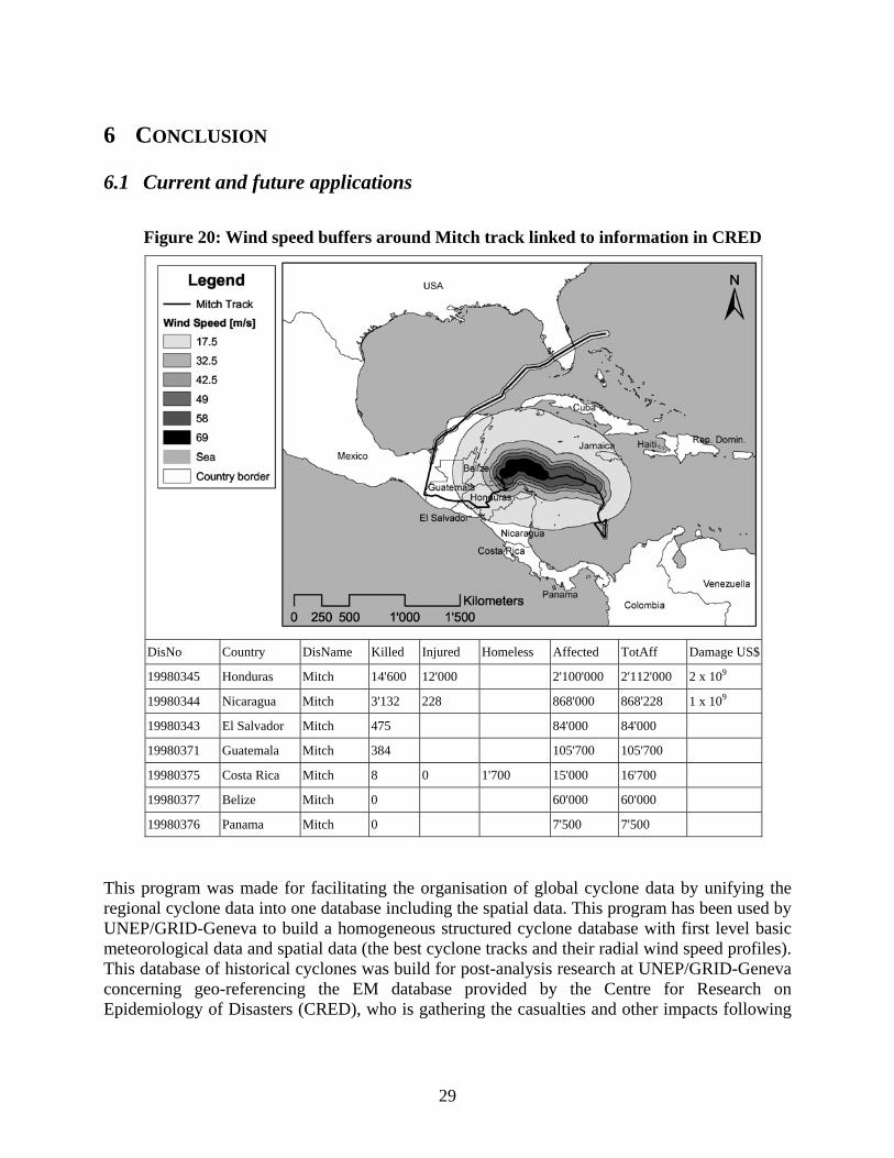
Figure 20: Wind speed buffers around Mitch track linked to information in CRED

DisNo Country DisName Killed Injured Homeless Affected TotAff Damage US$

19980345 Honduras Mitch 14'600 12'000 2'100'000 2'112'000 2 x 109

19980344 Nicaragua Mitch 3'132 228 868'000 868'228 1 x 109

19980343 El Salvador Mitch 475 84'000 84'000

19980371 Guatemala Mitch 384 105'700 105'700

19980375 Costa Rica Mitch 8 0 1'700 15'000 16'700

19980377 Belize Mitch 0 60'000 60'000

19980376 Panama Mitch 0 7'500 7'500

This program was made for facilitating the organisation of global cyclone data by unifying the regional cyclone data into one database including the spatial data. This program has been used by UNEP/GRID-Geneva to build a homogeneous structured cyclone database with first level basic meteorological data and spatial data (the best cyclone tracks and their radial wind speed profiles). This database of historical cyclones was build for post-analysis research at UNEP/GRID-Geneva concerning geo-referencing the EM database provided by the Centre for Research on Epidemiology of Disasters (CRED), who is gathering the casualties and other impacts following

30

disastrous events globally. For a global understanding on disasters, geo-referencing the different events is seen as an important approach. As illustrated in Figure 20, the affected population by the cyclone event Mitch is adequate to the region (including countries) that was befallen by the devastating cyclone. A more precise comparison was also carried out by using existing cyclone buffers in the Southern Hemisphere made by the Bureau of Meteorology in Australia. This comparison (see appendix D) illustrates an important correlation of our global modelling with the more precise regional cyclone observations. Further importance of a homogenised and combined database can be illustrated by the Atlantic Hurricane Database Re-analysis Project Documentation for 1851-85 Addition to the HURDAT Database (http://www.nhc.noaa.gov, 2002). This work has facilitated the post-analysis research (climatic change studies, seasonal forecasting, risk assessment for country emergency managers, analysis of potential losses, intensity forecasting techniques and verification of official and various model predictions of track and intensity) of all storms occurred in the Atlantic region.

6.2 Further developments As seen above, the aim with this study was obtained and the CycloneDatabaseManager concept has become useful for several purposes. It is nevertheless important to ameliorate this cyclone database procedure and this can be done in numerous ways: An important improvement for obtaining more precise and adequate results is to improve the cyclone data from the sources, and it’s above all a question of clarifying how the data has been retrieved and measured i.e. Metadata. • According to Holland G.J., 1980 the measured pressures observations are more conservative

and error prone than wind observations, but how reliable is this data? • The sustained maximum wind speed is less reliable than the values of central pressure and

this is probably due to the differences in measurement, that is not defined by the provider; • The most important uncertainty is the value of maxR that we were forced to estimate, since

relevant data were not to be found. In case of a better estimation of the above mentioned points we would be able to take further cyclone variables into account, e.g. landfall (vanishing of cyclone when it reaches the coast), surge (radical elevation of sea level and resulting in an enormous wave and consecutive flood) and rainband (precipitation around cyclone eye). These factors can be studied according to precise coast data. Another important improvement would be the transmission of the cyclone data between the provider and a centralised global database, where dynamic links could be created in order to establish an automatic data transmission. Buffer estimations could then be performed in real-time and could even help previsions. Such an organisation would need a better reporting network with more convenient data structure but also a common way of observing and reporting the cyclone events.

31

7 REFERENCES

Literature Anthes R. A., 1982, Tropical Cyclones –Their Evolution, Structure and Effects. American Meteorological Society Holland, G. J., 1987, Mature structure and structure change, In A global View of Tropical Cyclones, Elsberry, L. R., et al. Ed, 1987, Proceedings of the International workshop on Tropical Cyclones, (Bangkok, 1985). Holland, G. J., 1980: An analytic model of the wind and pressure profiles in hurricanes. Monthly Weather Review, 108, 1212-1218. American Meteorological Society Schloemer, R.W., 1954: Analysis and synthesis of hurricane wind patterns over Lake Okechobee. Florida. Hydromet. Rep., 31, Dept. of Commerce, Washington, DC, 49pp.

On the internet Holland, G. J., 1997: Horizontal Wind Structure, In Risk Prediction Initiave. Proceedings of the Workshop, Windfield Dynamics of Landfalling Tropical Cyclones, 28-30 May 1997. http://www.bbsr.edu/rpi/meetpart/land/landsum.html#holland2 Merrill, R. T., 2000: CH. 2: TROPICAL CYCLONE STRUCTURE In Global Guide to Tropical Cyclone Forecasting Holland G. J. et al. Ed. Bureau of Meteorology Research Centre. Melbourne, Australia http://www.bom.gov.au/bmrc/pubs/tcguide/ch2/ch2_4.htm Science And Technology Trends (SAIC), 1999: Crisis prediction disaster management Swiatek, Joseph A. et al. Ed. Revised by Dean C. Kaul, June 24, 1999 http://www.saic.com/products/simulation/cats/VUPQPV4R.pdf Landsea. C.W. et al., 2000 :The Atlantic Hurricane Database Re-analysis Project Documentation for 1851-85 Addition to the HURDAT Database http://www.nhc.noaa.gov/pastall.html and http://www.aoml.noaa.gov/hrd/hurdat/Documentation.html#Introduction

32

Personal Contacts by email Holland G.J., July 2001: Bureau of Meteorology Research Centre. Melbourne, Australia Harper B., July 2001: Bureau of Meteorology Research Centre. Melbourne, Australia Mark D. P., July 2001: The National Oceanic and Atmospheric Administration (NOAA), USA Leslie.Weiner-Leandro, July 2001: Federal Emergency Management Agency (FEMA), USA