Cycling to School: Increasing Secondary School Enrollment for Girls in India

Karthik Muralidharan†

Nishith Prakash

16 September 2016

Abstract: We study the impact of an innovative program in the Indian state of Bihar that aimed to reduce the gender gap in secondary school enrollment by providing girls who continued to secondary school with a bicycle that would improve access to school. Using data from a large representative household survey, we employ a triple difference approach (using boys and the neighboring state of Jharkhand as comparison groups) and find that being in a cohort that was exposed to the Cycle program increased girls' age-appropriate enrollment in secondary school by 32% and reduced the corresponding gender gap by 40%. We also find an 18% increase in the number of girls who appear for the high-stakes secondary school certificate exam, and a 12% increase in the number of girls who pass it. Parametric and non-parametric decompositions of the triple-difference estimate as a function of distance to the nearest secondary school show that the increases in enrollment mostly took place in villages that were further away from a secondary school, suggesting that the mechanism of impact was the reduction in the time and safety cost of school attendance made possible by the bicycle. We also find that the Cycle program was much more cost effective at increasing girls' secondary school enrollment than comparable conditional cash transfer programs in South Asia.

JEL Codes: H42, I21, J16, O15

Keywords: Conditional transfers, school access, gender gaps, bicycle, girls' education, female education, female empowerment, India, Bihar, MDG

† Karthik Muralidharan: UC San Diego, NBER, BREAD, J-PAL; E-mail: kamurali@ucsd.edu Nishith Prakash: University of Connecticut, IZA, and CReAM; E-mail: nishith.prakash@uconn.edu This project greatly benefited from financial and logistical support from the International Growth Center (IGC) for the research as well as its dissemination. We also thank the Department of Education, Government of Bihar for support with the data collection. We are especially grateful to Andrew Foster for his suggestions on this paper. We further thank Harold Alderman, Kate Antonovics, Mehtabul Azam, Chris Barrett, Eli Berman, Sonia Bhalotra, Prashant Bharadwaj, Aimee Chin, Jeff Clemens, Julie Cullen, Gordon Dahl, Jishnu Das, Eric Edmonds, Delia Furtado, Maitreesh Ghatak, Roger Gordon, Shaibal Gupta, Gordon Hanson, Edward Hoang, Scott Imberman, Chinhui Juhn, Santosh Kumar, Mushfiq Mobarak, Anjan Mukherji, Paul Niehaus, Emily Oster, Marc Rockmore, Andres Santos, Abhirup Sarkar, Anjani Kumar Singh, and various seminar participants for helpful comments and suggestions. Jay Prakash Agarwal, Abhishek Choudhary, Elizabeth Kaletski, and Michael Levere provided excellent research assistance.

1

"Investment in girls' education may be the highest-return investment available in the developing world."

Lawrence H. Summers (while Chief Economist of the World Bank)

"I think the bicycle has done more to emancipate women than anything else in the world."

Susan B. Anthony (19th century leader of US women's suffrage movement)

Introduction

Reducing gender gaps in school enrollment has been one of the most important goals for

international education policy over the past decade, and was one of the eight United Nation's

Millennium Development Goals (MDG's).1 While considerable progress has been made in

reducing gender gaps in primary schooling, there continue to be significant gaps in secondary

schooling, with a noticeable increase in adolescent years (Figure 1 – Panel A). It is therefore of

considerable economic and policy interest to identify cost-effective and scalable strategies for

increasing secondary school enrollment and completion rates for girls in developing countries.

Policies to improve female educational attainment in developing countries have focused on

both increasing the immediate benefits of schooling to families as well as on reducing the costs

of attending school. The most commonly used demand-side intervention to increase female

schooling has been to provide conditional cash transfers (CCTs) to households for keeping girls

enrolled in school. Several well-identified studies of CCT programs have found a positive

impact on girls' school enrollment and attainment (Fiszbein and Schady 2009).2 However, they

have not been found to be a very cost effective way of improving girls' schooling attainment,

perhaps because CCT programs typically aim to also provide income support to the poor and not

only to increase girls' schooling (Dhaliwal et al. 2013; Pritchett 2012).

On the supply side, the most common policy measure has been to improve school access by

constructing more schools and thereby reducing the distance cost of attending school. While

1 This policy priority is supported both on intrinsic grounds following the capabilities framework (Sen 1993, Nussbaum 2011) as well as on instrumental grounds following a vast body of prior research showing the benefits of increasing female education rates on several outcomes including lower infant, child, and maternal mortality; improved human capital transmission to children; and greater female labor force participation and income generation capacity. The World Development Report 2012 on "Gender Equality and Development" (World Bank 2011) summarizes the latest research on progress towards and benefits of gender equality. 2 There is a vast literature on the impact of CCT programs on education, health, and other outcomes in developing countries. References include Schultz (2004), Filmer and Schady (2011), Baird et al. (2011), and Barrera-Osorio et al. (2011). Fiszbein & Schady (2009) provide a good review of this literature.

2

well-identified studies of the impact of school construction programs have found positive effects

on enrollment (Duflo 2001; Burde and Linden 2013; Kazianga et al. 2013), there is a trade-off

between school access and scale. This trade-off may be particularly relevant for secondary

schools because they need qualified teachers for many subjects and expensive infrastructure like

laboratories, which require a minimum scale to be cost effective. Thus, while improving school

access has proven to be effective at increasing school participation, it is not obvious that

improving access should always take the form of constructing new schools.

In this paper, we evaluate the impact of an innovative program in the Indian state of Bihar

(launched in 2006) that aimed to improve secondary school access for girls without additional

school construction. The program provided all girls who enrolled in grade 9 with funds to buy a

bicycle to make it easier to access schools. The 'Cycle program' was therefore a 'conditional kind

transfer' (CKT) and had features of both demand and supply-side interventions. The enrollment

conditionality is analogous to demand-side CCT programs, but the bicycle also improves school

access by reducing the time, distance, and safety cost of attending school, which are features of

supply-side interventions. The program has proven to be politically popular and has been

replicated in other states across India, but there has been no credible estimation of its impact.

The main challenge for identification of program impact is that it was launched across the

full state of Bihar at a time of rapid growth, and sharp increases in public spending on education.

Thus, the large increases in girls' secondary school enrollment during this period (which policy

makers cite as evidence of positive program impact) could simply reflect broader trends and not

be in any way caused by the Cycle program. We address this identification challenge by

employing a triple difference strategy using a large representative household survey conducted in

2007-08 (18 months after the launch of the Cycle program) that included household roster data

with the education history of all residents.

We follow Duflo (2001) and treat older cohorts (aged 16 and 17) who were not exposed to

the Cycle program when they were making the transition to secondary school as the control

group and younger cohorts (aged 14 and 15) who were exposed to the program during this

transition as the treatment group. To account for omitted variables such as economic growth and

education spending, we compare changes in girls' secondary school enrollment across these

cohorts to changes in boys' enrollment for the same cohorts (as in Jayachandran and Lleras-

3

Muney 2009). However, since we reject the assumption of parallel pre-program trends in boys'

and girls' enrollment, we compare this double difference estimate in the state of Bihar (the

treated state), with the same estimate for the neighboring state of Jharkhand, which was part of

the state of Bihar for over 50 years, and only separated administratively in 2001. This triple

difference is our preferred estimate of program impact (since we do not reject parallel trends).

Our main result is that being in a cohort exposed to the Cycle program increased the

probability of a girl aged 14 or 15 being enrolled in or having completed grade 9 by 32% (a 5.2

percentage point increase on a base age-appropriate enrollment rate of 16.3 percent). Further, the

program also bridged the pre-existing gender gap in age-appropriate secondary school

enrollment between boys and girls (of 13 percentage points) by 40%. However, while this triple

difference estimate can plausibly be attributed to the Cycle program, we still cannot rule out the

possibility that the estimate is confounded by other factors that changed at the same time (such as

differential trends in returns to education for girls across the states after 2006).

We address this concern by noting that the causal impact of the Cycle program should vary

by the distance to a secondary school. We compare the triple difference estimate across villages

above and below the median distance to a secondary school (3km), and find that all the

enrollment impacts are found in villages that are 3km or further away from a secondary school.

We also plot the triple difference non-parametrically as a function of distance to the nearest

secondary school, and find that the treatment effect has an inverted-U shape. This is exactly what

would be expected from a model where the bicycle reduces the cost of attending school

proportional to the distance to school, but where the absolute cost of attendance is still too high

to attend at very large distances.

This is our most important result, because the inverted-U pattern of the treatment effect as a

function of distance to a secondary school is unlikely to be explained by omitted variables.3

Further, our finding close to zero impacts on enrollment for girls who lived near a secondary

school suggest that the magnitude of the triple difference estimate is not confounded by omitted

3 One further concern could be that other complementary investments such as improvements in roads, and law and order may also differentially benefit girls as a function of distance to school and thereby generate the same pattern. We address this concern by conducting a placebo test on the enrollment of eighth-grade girls (who are just one year younger, but were not eligible for the Cycle program), and find no effect here. See section 5.2 for details.

4

variables that may have raised girls' secondary school enrollment in Bihar in the same time

period. While the Cycle program had several components (including public ceremonies for

distribution of funds and an enrollment conditionality), this result also suggests that the main

mechanism of program impact was the reduction of the distance cost of attending school.

Turning to learning outcomes, we find using a similar triple-difference approach that in

cohorts exposed to the Cycle program, the number of girls appearing for the secondary school

certificate (SSC) exam increased by 18%, and find a 12% increase in the number of girls who

pass the exam. These results suggest that exposure to the Cycle program not only increased

enrollment on paper, but also increased the number of girls who stayed in secondary school to

the point of being able to take and pass the high-stakes SSC exam.

We find that the Cycle program was much more cost effective in increasing female school

enrollment than comparable CCT programs in South Asia. Possible reasons include: (a) requiring

the transfer to be spent on the bicycle made it more likely that the entire transfer would 'stick' to

the targeted girl as opposed to simply augmenting the household budget, (b) the design of the

program require the resources earmarked for the transfer to be spent in a way that alleviated not

just a demand constraint, but also an access constraint by reducing the daily cost of school

attendance – unlike typical cash transfer programs, and (c) the publicly coordinated provision of

bicycles to all girls in secondary school may have generated positive externalities including

increased safety from girls cycling to school in groups, greater demand for schooling from girls

on seeing their peers with a bicycle, and a relaxation of patriarchal social norms against

adolescent girls traveling outside the village to attend school (see discussion in section 6).

The possibility of such spillovers highlights the value of evaluating the cycle program at

scale, because even experimental evaluations of smaller programs may not yield the relevant

policy parameter of interest (which includes the spillovers from a scaled up implementation).

Methodologically, our approach illustrates the feasibility of credible impact evaluations in

developing countries even in the context of such a universal program roll out at scale.

Specifically, the analysis of differential impact of the Cycle program as a function of distance to

a secondary school is similar to the approaches employed in Bleakley (2007) and Hornbeck

(2010) in historical contexts where pre-existing cross-sectional heterogeneity is used to predict

5

differential 'effective impact' of a universally implemented program (de-worming) or broadly

available new technology (barbed wire).

From a policy perspective, it is worth highlighting that we evaluate an 'as is' implementation

of a program that was scaled up across a state with over 100 million people, and a history of high

levels of corruption in public programs. Given a setting with weak state capacity for program

implementation, it is worth noting that the Cycle program had important features that enabled it

to be implemented remarkably effectively, with only 5% of eligible beneficiaries not receiving a

bicycle (see section 2). Thus, the Cycle program appears to have been quite effective in

providing a non-fungible transfer to girls that was not captured by either officials or households,

and also reduced the daily cost of school attendance for girls. The large positive effects of the

Cycle program on increasing female secondary school enrollment and in reducing the gender

gap, its relative ease of implementation, its cost effectiveness, and its high visibility and political

popularity suggest that this may be a promising policy option to boost female secondary school

enrollment in other developing country settings as well.

The rest of this paper is organized as follows. Section 2 describes the context and the

program; section 3 describes the data, estimating equations, and identification assumptions;

section 4 presents the main results; section 5 presents several important robustness checks;

section 6 discusses cost effectiveness and the broader implications of our results for debates on

cash versus kind transfers; section 7 concludes.

2. Context and Program Description

Bihar is the third most populous state in India, with a population of over 100 million. At the

turn of the century, Bihar was one of the most economically backward states of India and also

had among the lowest mean levels of education (Desai et al. 2010). In addition, the gender gap

in educational attainment is even more pronounced in Bihar relative to the all India figures

(Figure 1 – Panel A). The drop off in girls' enrollment is particularly pronounced at ages 14 to

15, which is around the age of puberty and also the age of transition to secondary schooling.

An important barrier to secondary school enrollment is distance and the probability of being

enrolled in or having completed grade 9 (the first grade of secondary school) steadily declines as

the distance to the nearest secondary school increases (Figure 1 – Panel B). Distance to school is

6

also a more salient constraint for secondary school relative to primary school.4 While nearly 90%

of villages in Bihar had a primary school as of late 2007, less than 12% of them had a secondary

school (Table A.1). While there is an ongoing national program to improve access to secondary

schooling via school construction and expansion, this is an expensive and ongoing process and

can only slowly reach children who are currently far from a secondary school.

Following over a decade of weak performance on several measures of governance and

human development, the newly elected state government in Bihar (in late 2005) prioritized

improvements in law and order, and service delivery in the social sector and undertook several

initiatives to improve education (Chakrabarti 2013). A particularly prominent program that the

Government of Bihar (GoB) launched in 2006 was the Chief Minister's Bicycle program

(hereafter referred to as the Cycle program) that provided girls who enrolled in secondary school

(grade 9) with a free bicycle to enable them to get to school more easily.

The GoB did not directly procure bicycles, but disbursed funds (Rs. 2,000/student; ~$45 at

2006 exchange rates) to eligible female students to purchase a bicycle. The funds were

distributed through schools in public ceremonies attended by local officials and elected

representatives, and the GoB required school principals to collect the receipts and provide a

utilization certificate showing that the funds were used to purchase a bicycle. The program was

designed this way to provide households with some flexibility in the type of bicycle they bought,

and to obviate the need for the government to get involved in large-scale procurement and

distribution of bicycles. But the program was explicitly designed to be a conditional kind transfer

(CKT) of a bicycle to be used by the eligible girl, as opposed to the more typical conditional cash

transfer (CCT) programs used to reward parents and households for sending their daughters to

school. Thus, while there are similarities between the Cycle program and typical CCT programs

(they both provide a transfer to households conditional on school participation), the design of the

Cycle program featured important innovations relative to typical CCT programs by earmarking

the transfer to be spent in a way that would not just increase household demand for girls'

4 The school system in Bihar (and many states in India) is organized as primary school (grades 1-5), upper primary or middle-school (grades 6-8), secondary (grades 9-10), and higher secondary (grades 11-12).

7

secondary education5 but also alleviate the access constraint to secondary schooling for girls by

reducing the daily cost of going to school.

However, while well-intentioned, it was not obvious that the program would reach its

intended beneficiaries. As of 2005, multiple studies pointed to Bihar having among the poorest

indicators of service delivery in India, and also among the lowest levels of female education

suggesting low household demand for girls' education.6 Thus, the Cycle program could have

failed to have an impact either due to government implementation failures such as non-delivery

of funds to parents or delayed/reduced payments due to corruption or administrative inefficiency;

or due to household behavioral responses such as parents taking the cash and providing fake

receipts showing bicycle purchase or using the funds to buy a bicycle for household use but not

actually sending their daughters to schools (note that the program eligibility in 2006 to 2008 only

required enrollment in secondary school and did not verify attendance).

Since our main data come from a household health survey that was not designed to study the

bicycle program (see next section), we are unable to directly evaluate program implementation in

this paper. We therefore rely on a complementary study designed to study the implementation of

the Cycle program to provide evidence on the 'first stage' of the program. Using detailed

household surveys, Ghatak et al. 2016 find that the program was remarkably well implemented,

with only 3% of households with eligible beneficiaries not having received the cash to buy the

bicycles, and only 2% of households who received the cash not having purchased a bicycle.

Qualitative evidence suggests that the reasons for low leakage in the Cycle program

included:7 (a) universal eligibility - every girl in 9th grade was entitled to the bicycle grant,

which removed officials' discretion in determining beneficiaries; (b) the one-time nature of the

transfer, which made it easier to monitor than smaller regular transfers; (c) public ceremonies for

awarding the cash to purchase bicycles in schools, which created social pressure against parents

5 Note that other members of the households would also benefit from the bicycle outside school hours. Thus, the non-education benefits of the Cycle program for the rest of the household would still be positive (though perhaps not as much as that from an unconstrained augmentation of the household budget as in typical CCT programs). 6 Kremer et al (2005) report that 38% of public-school teachers in Bihar were absent on any given day in 2003 (the second-highest rate across Indian states). The Planning Commission of India’s estimates in 2005 found that Bihar was the state with the highest rate of leakage (exceeding 75%) in the national food security program (PEO 2005). Statistics on low female education attainment in Bihar are available in Desai et al. 2010 (also see Figure 1) 7 Sources include discussions by the authors with senior policy makers, local officials, and head-teachers, as well as prior qualitative studies (such as Debroy 2010, Nayar 2012, and Ghatak et al. 2016).

8

taking the cash and not purchasing bicycles (or reselling them); (d) the demographic group

eligible for the benefit (households with girls enrolled in secondary school) was more

empowered relative to the more disadvantaged recipients of other public programs, making it

more difficult for officials to deny them benefits; and (e) commitment of the political leadership

of the state towards the program, which was highly visible to the public and politically salient.

Nevertheless, even though the Cycle program was well implemented, it is possible that it did

not have much of a causal impact on the stated objective of increasing girls' secondary school

enrollment. In particular, given the sharp increase in Bihar’s growth rate and in its public

education spending starting in 2006, the large post-2006 increases in girls' secondary-school

enrollment, may have taken place regardless of the Cycle program. Thus, even though the Govt.

of Bihar spent Rs. 310 million ($7 million) to provide funds for bicycles for 160,000 girls in

2007-08 (Govt. of Bihar budget documents) it is possible that this benefit was mostly provided to

infra-marginal girls who would have enrolled in secondary school anyway, and that there was

limited marginal impact of the Cycle program on female secondary school enrollment.

3 Data, Identification Strategy, and Estimating Equations

3.1. Data

Our main data source is the third wave of the Indian District Level Health Survey (DLHS-3)

conducted in 2007-08. The DLHS-3 is nationally representative and is one of the largest

household surveys ever carried out in India, with a sample size of around 720,000 households

across 601 districts in India. The data includes household socio-economic characteristics, and a

roster of all members in the household, their education attainment, and current schooling status.

In addition, the village-level questionnaire in the DLHS includes information on all educational

facilities available in the village, and the distance to the nearest educational facility of each type

that is not available in the village (including primary, middle, and secondary schools).

The timing of the DLHS-3 is ideal for our analysis, since it was conducted around 18 months

after the Cycle program was launched.8 Since the typical age at which students enter grade nine

(the first year of secondary school) is 14 or 15, household members who are 16 or 17 years old

8 The program was launched in the school year 2006-07 (which started in June 2006), while the DLHS was conducted in late 2007 and early 2008 (in the middle of the 2007-08 school year).

9

would not have been exposed to the program when they were deciding on whether to continue to

secondary school, while those who are currently 14 or 15 would have been eligible for the

program. This enables us to treat 14-15 year olds as 'treated' cohorts and 16-17 year olds as

'control' cohorts (as in Duflo 2001). Thus, our estimation sample uses households that have at

least one member aged 14 to 17 living in the states of Bihar and Jharkhand.

We also use two other datasets in this paper. First, we collect school-level secondary school

enrollment data by gender for both Bihar and Jharkhand. We do not use this data for estimating

treatment effects, since schools may inflate enrollment figures in response to the program.9 We

only use this data from the years prior to the launch of the program (2002 to 2006) to test for

parallel trends in the growth rate of enrollment of boys and girls in Bihar and Jharkhand.

Second, to study the impact on learning outcomes, we collect official data on the number of

students who appeared in and passed the secondary school certificate (SSC) examination in both

Bihar and Jharkhand. This data comes from the official state exam boards and only reflects those

students who actually took the exam and were graded for it, and is hence much more reliable

than school-based enrollment records that will often show students as enrolled who may not be

attending school much. The exam data (from the official exam board) cannot be similarly

inflated. Note that neither of these two datasets includes information on the distance to the

nearest school for individual students, and so we can only study heterogeneity of impact by

distance in the DLHS-3 household data. However, we need the annual school-level data to test

for parallel trends because the DLHS-3 is only collected at one point in time.

3.2. Identification Strategy and Estimating Equations

3.2.1 Triple Difference Estimate

Our main outcome of interest is whether a student is enrolled in or has completed grade nine

(the first year of secondary school). The first difference compares this outcome across girls aged

14 or 15 in Bihar (the 'treated' cohort) and girls aged 16 or 17 in Bihar (the 'control' cohort).

Since this difference is likely to be confounded by the several other changes taking place in

9 Distorting school records in response to incentives is not uncommon in India, and has also been documented in other settings such as school feeding programs in India (Linden and Shastry 2012). School-level data is also not ideal for testing program impacts on enrollment because of the likely differences in school construction across the two states after 2005-06. Hence, household survey data are better suited for our analysis.

10

Bihar during the same period, we use boys of the same ages in Bihar as a control group. As in

Jayachandran and Lleras-Muney (2009), boys serve as an especially useful control group for the

Cycle program, because they would have been exposed to all the other changes that were taking

place in Bihar during the period of interest (including increasing household incomes and

increased public investment in education), but were not eligible for this program. However,

since girls' enrollment rate was much lower to begin with, it is possible that their enrollment was

growing faster than that of boys. We test for parallel trends in boys' and girls' enrollment growth

in the four years prior to the program (2002-03 to 2005-06) using official enrollment data, and

reject the null hypothesis of parallel trends (Table 1 - Panel A).

We therefore construct a triple difference (DDD) estimate of program impact by comparing

the double difference (as computed above) in the state of Bihar with the same double difference

in the neighboring state of Jharkhand (which did not have the Cycle program). The use of

Jharkhand as a comparison group for Bihar is especially credible since the two states were part of

the unified state of Bihar until 2001 and were only administratively bifurcated into two states in

2001. Thus, the governance structure of the two states was identical until 2001, and the quality

of governance in the two states was comparable for a few years after the bifurcation.10 We test

for parallel trends in the triple difference in the period 2002-03 to 2005-06, and find that we do

not reject the null hypothesis of parallel trends, with the coefficient on the triple interaction term

being close to zero (Table 1 - Panel B).11

The triple-difference estimate of exposure to the Cycle program is estimated by:

𝑦𝑦𝑖𝑖ℎ𝑣𝑣 = 𝛽𝛽0 + 𝛽𝛽1 ∙ 𝐹𝐹𝑖𝑖ℎ𝑣𝑣 ∙ 𝑇𝑇𝑖𝑖ℎ𝑣𝑣 ∙ 𝐵𝐵𝐵𝐵𝑖𝑖ℎ𝑣𝑣 + 𝛽𝛽2 ∙ 𝐹𝐹𝑖𝑖ℎ𝑣𝑣 ∙ 𝐵𝐵𝐵𝐵𝑖𝑖ℎ𝑣𝑣 + 𝛽𝛽3 ∙ 𝑇𝑇𝑖𝑖ℎ𝑣𝑣 ∙ 𝐵𝐵𝐵𝐵𝑖𝑖ℎ𝑣𝑣 + 𝛽𝛽4 ∙ 𝐹𝐹𝑖𝑖ℎ𝑣𝑣 ∙ 𝑇𝑇𝑖𝑖ℎ𝑣𝑣 +

𝛽𝛽5 ∙ 𝐹𝐹𝑖𝑖ℎ𝑣𝑣 + 𝛽𝛽6 ∙ 𝑇𝑇𝑖𝑖ℎ𝑣𝑣 + 𝛽𝛽7 ∙ 𝐵𝐵𝐵𝐵𝑖𝑖ℎ𝑣𝑣 + 𝜀𝜀𝑖𝑖ℎ𝑣𝑣 (1)

where 𝑦𝑦𝑖𝑖ℎ𝑣𝑣 is the outcome variable of interest corresponding to child i, in household h and

village v. 𝐹𝐹𝑖𝑖ℎ𝑣𝑣 is an indicator for being female, 𝑇𝑇𝑖𝑖ℎ𝑣𝑣 is an indicator for being in a 'treated' cohort

10 Kremer et al. 2005 show that Bihar and Jharkhand had the second highest and highest rates of teacher absence across 19 Indian states in 2003, and were not significantly different from each other. 11 We have school-level enrollment data for all schools in Bihar (where the GoB facilitated data collection), but in Jharkhand we only have data for the 10 districts that border Bihar (out of a total of 24), since field teams had to to visit each district to collect this data. Thus, analysis of parallel trends is based on using all districts in Bihar and border districts in Jharkhand, while the main analysis (using the DLHS data) uses all the districts in Bihar and Jharkhand. We show later that restricting the main analysis using the DLHS data to only the border districts yields similar estimates of the treatment effects (section 5.3).

11

(being aged 14 or 15), and 𝐵𝐵𝐵𝐵𝑖𝑖ℎ𝑣𝑣 is an indicator for an observation from Bihar. The estimation

sample includes all members of the household roster in surveyed households aged 14 to 17 in

Bihar and Jharkhand, and the omitted category of 16 and 17 year olds correspond to the 'control'

cohorts. The main parameter of interest is 𝛽𝛽1(the triple-difference estimate), and 𝛽𝛽2 through 𝛽𝛽7

are the estimates of the double interaction terms and linear terms respectively.12 Standard errors

are clustered at the village-level.

Note that the test for parallel trends uses school-level enrollment data and has to be estimated

in logs and not levels because the population base and distribution of school size in Bihar and

Jharkhand are different. However, parallel trends in logs (which implies equal growth rates) does

not imply that parallel trends will also hold in levels unless the base enrollment rate is similar.

We see in Table A.1 that secondary school participation for control-cohort girls was a little lower

in Bihar (28%) than in Jharkhand (36%), and it was nearly identical for boys (48% vs. 47%).

Hence, the parallel trends in logs prior to the reform would have implied a slightly larger annual

percentage point increase in girls' enrollment in Jharkhand in the pre-period.13 The triple-

difference estimates in (1), which measures the impact on percentage points of enrollment, are

therefore likely to be a lower bound on the true impact of exposure to the Cycle program on girls'

secondary school enrollment.

Table A.1 presents summary statistics in the estimation sample, and we see some significant

differences between Bihar and Jharkhand – especially shares of disadvantaged scheduled castes

and tribes, with the latter having a much larger share of the tribal population. We account for

these differences by estimating Eq. (1) with a progressively rich set of controls for demographic,

12 We also tried to estimate the 'first stage' of the Cycle program in the DLHS data using this same triple difference specification. However, the DLHS only asks if a household owns a bicycle and not the number of bicycles in the household or who owns them. Since over 70% of households in the sample own a bicycle, this test is underpowered and we find positive but insignificant effects on the incidence of household-level bicycle ownership. Since the detailed household survey conducted by Ghatak et al. (2016) was explicitly undertaken to study the implementation of the Cycle program, we rely on their results to infer that almost all eligible girls did in fact receive a bicycle. 13 Ideally, we would be able to show both parallel trends and treatment effects in levels or logs. Unfortunately, the DLHS data is only a single cross-section and cannot be used to test for parallel trends. Parallel trends with school data have to be shown in logs because the population base and average school size across states is different. However, the school data is both incomplete and not-reliable for estimating treatment effects (as explained earlier). We do use school-level data for the exam results since these are independently verified data and available for the full state and show both parallel trends and treatment effects in logs for the exam results (see section 4.4).

12

socioeconomic, and village characteristics. We show 𝛽𝛽1 in each of these specifications, but focus

our discussion on the specifications with the full set of village and household controls.

3.2.3 Quadruple Difference Estimate

Despite the non-rejection of parallel trends for the triple difference (Table 1 - Panel B), the

estimate of estimate of in 𝛽𝛽1 Eq. (1) may potentially be confounded by omitted variables that

differentially affect the trend in girls' secondary school enrollment in Bihar relative to Jharkhand

after 2006 (such as faster growth in returns to education for girls). Further, it is useful to

examine the extent to which the mechanism of program impact (if any) can be attributed to the

conditionality versus the improvement in school access enabled by the bicycle.

We address these issues by noting that if the estimate of 𝛽𝛽1 in Eq. (1) is causal, we should

expect to see heterogeneous effects of the program as a function of the distance to the nearest

secondary school. Since the Cycle program would have reduced the 'distance cost' of attending

school, the triple difference should be larger in cases where a secondary school was further away

(if it is a causal estimate). Figure A.1 shows that the median village in Bihar was 3 kilometers

(km) away from a secondary school. We therefore define an indicator variable 𝐿𝐿𝐿𝐿𝑣𝑣 ('Long

Distance') that takes the value 1 if a village is 3km or further away from a secondary school, and

estimate a quadruple difference using the specification:

𝑦𝑦𝑖𝑖ℎ𝑣𝑣 = 𝛽𝛽0 + 𝛽𝛽1 ∙ 𝐹𝐹𝑖𝑖ℎ𝑣𝑣 ∙ 𝑇𝑇𝑖𝑖ℎ𝑣𝑣 ∙ 𝐵𝐵𝐵𝐵𝑖𝑖ℎ𝑣𝑣 ∙ 𝐿𝐿𝐿𝐿𝑣𝑣 + ∑ 𝛽𝛽𝑖𝑖52 ∙ (4 𝑇𝑇𝑇𝑇𝑇𝑇𝑇𝑇𝑇𝑇𝑇𝑇 𝐼𝐼𝐼𝐼𝐼𝐼𝑇𝑇𝑇𝑇𝐼𝐼𝐼𝐼𝐼𝐼𝑇𝑇𝐼𝐼𝐼𝐼𝐼𝐼) + ∑ 𝛽𝛽𝑖𝑖11

6 ∙

(6 𝐿𝐿𝐼𝐼𝐷𝐷𝐷𝐷𝑇𝑇𝑇𝑇 𝐼𝐼𝐼𝐼𝐼𝐼𝑇𝑇𝑇𝑇𝐼𝐼𝐼𝐼𝐼𝐼𝑇𝑇𝐼𝐼𝐼𝐼𝐼𝐼) + ∑ 𝛽𝛽𝑖𝑖1512 ∙ (4 𝐿𝐿𝑇𝑇𝐼𝐼𝑇𝑇𝐼𝐼𝑇𝑇 𝑇𝑇𝑇𝑇𝑇𝑇𝑇𝑇𝐼𝐼) + 𝜀𝜀𝑖𝑖ℎ𝑣𝑣 (2)

where 𝛽𝛽1is the parameter of interest, and indicates the extent to which the triple difference

estimate in Eq. (1) is differentially coming from villages further away from a secondary school.

The estimation sample, controls, and clustering are as in Eq. (1).

3.2.4 Non-Parametric Triple Difference Estimate (DDD by Distance to Secondary School)

We enrich the analysis above by non-parametrically plotting the triple difference estimate in

Eq. (1) as a function of the distance to the nearest secondary school. The benefits of school

attendance are less likely to depend on the distance to school while the costs can be thought of as

13

linear in travel time (see Figure A.2).14 The provision of a cycle would therefore reduce the cost

of school attendance proportional to the original distance from the nearest secondary school.

Figure A.2 illustrates that if the estimate of 𝛽𝛽1in Eq. (1) is causal, we would expect the impact to

be low in villages where there is a secondary school nearby (since the marginal impact of the

cycle would be low) or where the secondary school is very far away (since the absolute cost of

attending school would still be too high), and highest at intermediate distances.

3.2.5 Estimate of Program Impact on Learning Outcomes

We estimate the impact of the Cycle program on learning outcomes using official tenth-grade

board exam results for both Bihar and Jharkhand. Focusing on the impact of the program on the

percentage of students who pass these exams will be misleading if academically weaker students

are now more likely to go to secondary school and attempt the exam. We therefore focus our

analysis on the logarithm of the absolute number of students who attempt and pass the tenth-

grade exams, using a triple difference estimate similar to Eq. (1).

4. Results

4.1. Enrollment Impact

The triple-difference estimates of the impact of the Cycle program, based on Eq. (1) are

presented in Table 2.15 The estimates with no controls and with demographic controls (columns

1 and 2) suggest a program impact on 9th grade enrollment (or completion) of 11-12 percentage

points, while including controls for household education and assets reduces the estimate to 5.2

percentage points, with no further change from including village-level controls (columns 3 and

4). Two points are worth noting.

14 We abstract from the costs of school attendance that do not vary by distance (such as the opportunity cost of time spent in school) and focus only on those that do vary by distance, which are likely to be affected by the provision of the cycle. Note that the benefits of schooling do not have to be invariant to the distance to a school (as shown in Figure A.2). The identification strategy will be valid as long as the slope of the cost of school attendance with respect to distance is steeper than the slope of the benefits. 15 Results from estimating the double difference (comparing changes in enrollment for girls in Bihar with that for boys in Bihar) are shown in Table A.2 (note that these are only for completeness because we reject the parallel trends hypothesis for the double difference). We also use Table A.2 to show the coefficients on the control variables that are included as we progress from column 1 to 4. These coefficients are very similar in the triple and quadruple difference specifications and are not shown in later tables because they are not the focus of this paper.

14

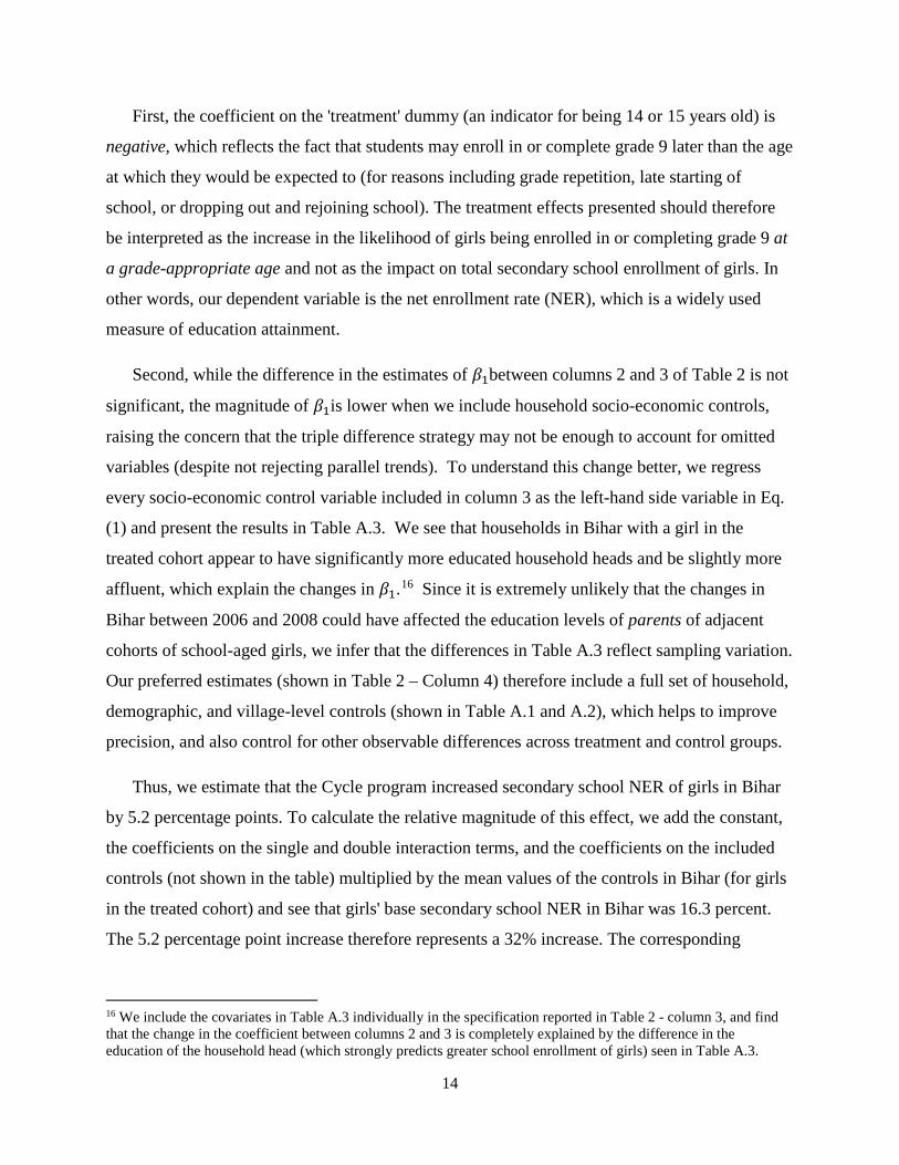
First, the coefficient on the 'treatment' dummy (an indicator for being 14 or 15 years old) is

negative, which reflects the fact that students may enroll in or complete grade 9 later than the age

at which they would be expected to (for reasons including grade repetition, late starting of

school, or dropping out and rejoining school). The treatment effects presented should therefore

be interpreted as the increase in the likelihood of girls being enrolled in or completing grade 9 at

a grade-appropriate age and not as the impact on total secondary school enrollment of girls. In

other words, our dependent variable is the net enrollment rate (NER), which is a widely used

measure of education attainment.

Second, while the difference in the estimates of 𝛽𝛽1between columns 2 and 3 of Table 2 is not

significant, the magnitude of 𝛽𝛽1is lower when we include household socio-economic controls,

raising the concern that the triple difference strategy may not be enough to account for omitted

variables (despite not rejecting parallel trends). To understand this change better, we regress

every socio-economic control variable included in column 3 as the left-hand side variable in Eq.

(1) and present the results in Table A.3. We see that households in Bihar with a girl in the

treated cohort appear to have significantly more educated household heads and be slightly more

affluent, which explain the changes in 𝛽𝛽1.16 Since it is extremely unlikely that the changes in

Bihar between 2006 and 2008 could have affected the education levels of parents of adjacent

cohorts of school-aged girls, we infer that the differences in Table A.3 reflect sampling variation.

Our preferred estimates (shown in Table 2 – Column 4) therefore include a full set of household,

demographic, and village-level controls (shown in Table A.1 and A.2), which helps to improve

precision, and also control for other observable differences across treatment and control groups.

Thus, we estimate that the Cycle program increased secondary school NER of girls in Bihar

by 5.2 percentage points. To calculate the relative magnitude of this effect, we add the constant,

the coefficients on the single and double interaction terms, and the coefficients on the included

controls (not shown in the table) multiplied by the mean values of the controls in Bihar (for girls

in the treated cohort) and see that girls' base secondary school NER in Bihar was 16.3 percent.

The 5.2 percentage point increase therefore represents a 32% increase. The corresponding

16 We include the covariates in Table A.3 individually in the specification reported in Table 2 - column 3, and find that the change in the coefficient between columns 2 and 3 is completely explained by the difference in the education of the household head (which strongly predicts greater school enrollment of girls) seen in Table A.3.

15

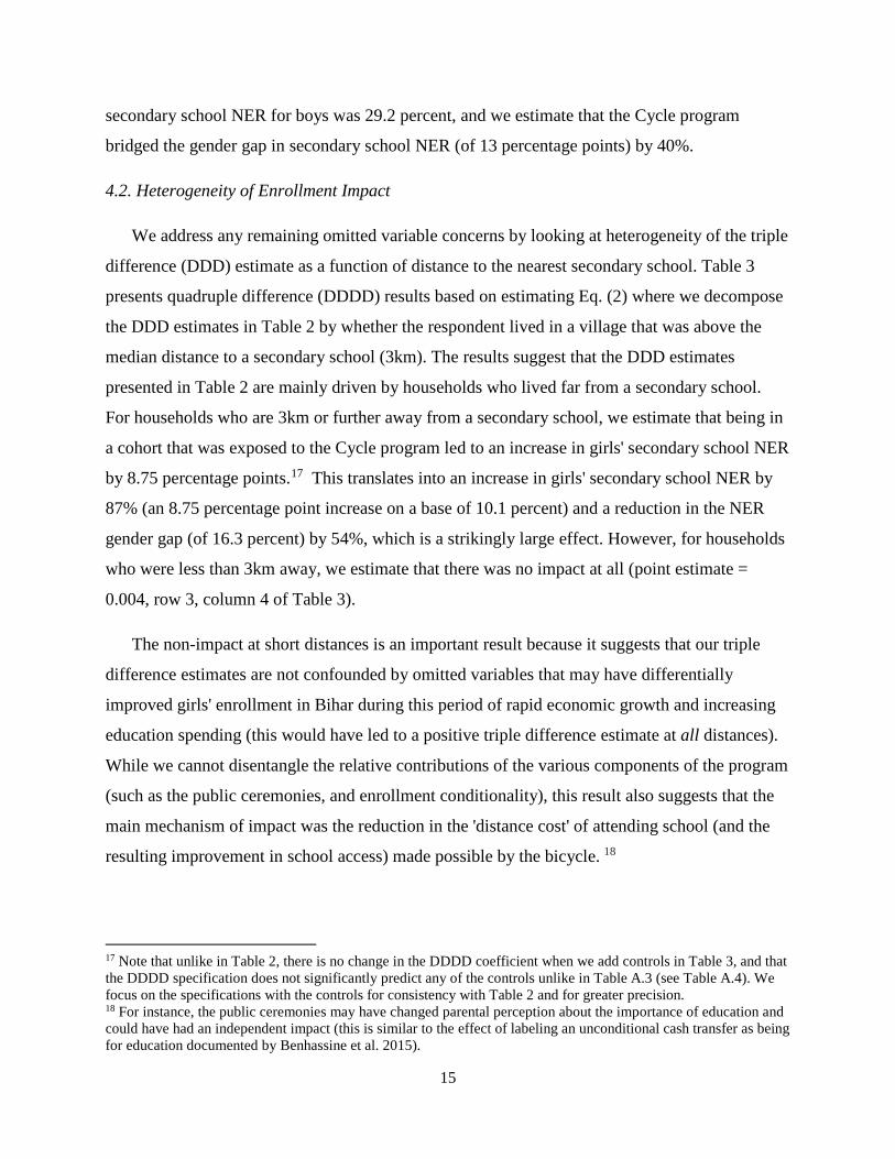
secondary school NER for boys was 29.2 percent, and we estimate that the Cycle program

bridged the gender gap in secondary school NER (of 13 percentage points) by 40%.

4.2. Heterogeneity of Enrollment Impact

We address any remaining omitted variable concerns by looking at heterogeneity of the triple

difference (DDD) estimate as a function of distance to the nearest secondary school. Table 3

presents quadruple difference (DDDD) results based on estimating Eq. (2) where we decompose

the DDD estimates in Table 2 by whether the respondent lived in a village that was above the

median distance to a secondary school (3km). The results suggest that the DDD estimates

presented in Table 2 are mainly driven by households who lived far from a secondary school.

For households who are 3km or further away from a secondary school, we estimate that being in

a cohort that was exposed to the Cycle program led to an increase in girls' secondary school NER

by 8.75 percentage points.17 This translates into an increase in girls' secondary school NER by

87% (an 8.75 percentage point increase on a base of 10.1 percent) and a reduction in the NER

gender gap (of 16.3 percent) by 54%, which is a strikingly large effect. However, for households

who were less than 3km away, we estimate that there was no impact at all (point estimate =

0.004, row 3, column 4 of Table 3).

The non-impact at short distances is an important result because it suggests that our triple

difference estimates are not confounded by omitted variables that may have differentially

improved girls' enrollment in Bihar during this period of rapid economic growth and increasing

education spending (this would have led to a positive triple difference estimate at all distances).

While we cannot disentangle the relative contributions of the various components of the program

(such as the public ceremonies, and enrollment conditionality), this result also suggests that the

main mechanism of impact was the reduction in the 'distance cost' of attending school (and the

resulting improvement in school access) made possible by the bicycle. 18

17 Note that unlike in Table 2, there is no change in the DDDD coefficient when we add controls in Table 3, and that the DDDD specification does not significantly predict any of the controls unlike in Table A.3 (see Table A.4). We focus on the specifications with the controls for consistency with Table 2 and for greater precision. 18 For instance, the public ceremonies may have changed parental perception about the importance of education and could have had an independent impact (this is similar to the effect of labeling an unconditional cash transfer as being for education documented by Benhassine et al. 2015).

16

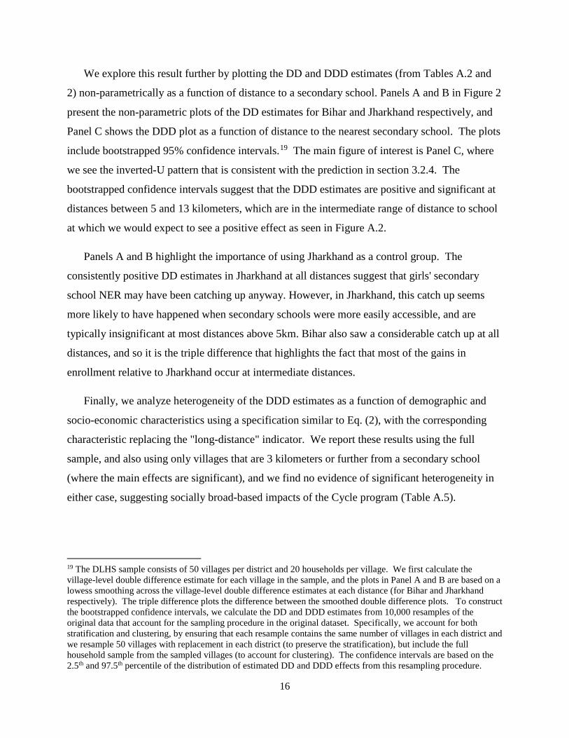
We explore this result further by plotting the DD and DDD estimates (from Tables A.2 and

2) non-parametrically as a function of distance to a secondary school. Panels A and B in Figure 2

present the non-parametric plots of the DD estimates for Bihar and Jharkhand respectively, and

Panel C shows the DDD plot as a function of distance to the nearest secondary school. The plots

include bootstrapped 95% confidence intervals.19 The main figure of interest is Panel C, where

we see the inverted-U pattern that is consistent with the prediction in section 3.2.4. The

bootstrapped confidence intervals suggest that the DDD estimates are positive and significant at

distances between 5 and 13 kilometers, which are in the intermediate range of distance to school

at which we would expect to see a positive effect as seen in Figure A.2.

Panels A and B highlight the importance of using Jharkhand as a control group. The

consistently positive DD estimates in Jharkhand at all distances suggest that girls' secondary

school NER may have been catching up anyway. However, in Jharkhand, this catch up seems

more likely to have happened when secondary schools were more easily accessible, and are

typically insignificant at most distances above 5km. Bihar also saw a considerable catch up at all

distances, and so it is the triple difference that highlights the fact that most of the gains in

enrollment relative to Jharkhand occur at intermediate distances.

Finally, we analyze heterogeneity of the DDD estimates as a function of demographic and

socio-economic characteristics using a specification similar to Eq. (2), with the corresponding

characteristic replacing the "long-distance" indicator. We report these results using the full

sample, and also using only villages that are 3 kilometers or further from a secondary school

(where the main effects are significant), and we find no evidence of significant heterogeneity in

either case, suggesting socially broad-based impacts of the Cycle program (Table A.5).

19 The DLHS sample consists of 50 villages per district and 20 households per village. We first calculate the village-level double difference estimate for each village in the sample, and the plots in Panel A and B are based on a lowess smoothing across the village-level double difference estimates at each distance (for Bihar and Jharkhand respectively). The triple difference plots the difference between the smoothed double difference plots. To construct the bootstrapped confidence intervals, we calculate the DD and DDD estimates from 10,000 resamples of the original data that account for the sampling procedure in the original dataset. Specifically, we account for both stratification and clustering, by ensuring that each resample contains the same number of villages in each district and we resample 50 villages with replacement in each district (to preserve the stratification), but include the full household sample from the sampled villages (to account for clustering). The confidence intervals are based on the 2.5th and 97.5th percentile of the distribution of estimated DD and DDD effects from this resampling procedure.

17

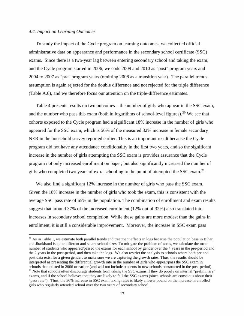
4.4. Impact on Learning Outcomes

To study the impact of the Cycle program on learning outcomes, we collected official

administrative data on appearance and performance in the secondary school certificate (SSC)

exams. Since there is a two-year lag between entering secondary school and taking the exam,

and the Cycle program started in 2006, we code 2009 and 2010 as "post" program years and

2004 to 2007 as "pre" program years (omitting 2008 as a transition year). The parallel trends

assumption is again rejected for the double difference and not rejected for the triple difference

(Table A.6), and we therefore focus our attention on the triple-difference estimates.

Table 4 presents results on two outcomes – the number of girls who appear in the SSC exam,

and the number who pass this exam (both in logarithms of school-level figures).20 We see that

cohorts exposed to the Cycle program had a significant 18% increase in the number of girls who

appeared for the SSC exam, which is 56% of the measured 32% increase in female secondary

NER in the household survey reported earlier. This is an important result because the Cycle

program did not have any attendance conditionality in the first two years, and so the significant

increase in the number of girls attempting the SSC exam is provides assurance that the Cycle

program not only increased enrollment on paper, but also significantly increased the number of

girls who completed two years of extra schooling to the point of attempted the SSC exam.21

We also find a significant 12% increase in the number of girls who pass the SSC exam.

Given the 18% increase in the number of girls who took the exam, this is consistent with the

average SSC pass rate of 65% in the population. The combination of enrollment and exam results

suggest that around 37% of the increased enrollment (12% out of 32%) also translated into

increases in secondary school completion. While these gains are more modest than the gains in

enrollment, it is still a considerable improvement. Moreover, the increase in SSC exam pass

20 As in Table 1, we estimate both parallel trends and treatment effects in logs because the population base in Bihar and Jharkhand is quite different and so are school sizes. To mitigate the problem of zeros, we calculate the mean number of students who appeared/passed the exams for each school by gender over the 4 years in the pre-period and the 2 years in the post-period, and then take the logs. We also restrict the analysis to schools where both pre and post data exist for a given gender, to make sure we are capturing the growth rates. Thus, the results should be interpreted as presenting the differential growth rate in the number of girls who appear/pass the SSC exam in schools that existed in 2006 or earlier (and will not include students in new schools constructed in the post-period). 21 Note that schools often discourage students from taking the SSC exams if they do poorly on internal "preliminary" exams, and if the school believes that they are likely to fail the SSC exams (since schools are conscious about their “pass rate”). Thus, the 56% increase in SSC exam taking rates is likely a lower bound on the increase in enrolled girls who regularly attended school over the two years of secondary school.

18

rates is a credible measure of increased human capital accumulation, because the SSC exam is

the first externally-evaluated credential of learning outcomes in the Indian schooling system.

5. Robustness

5.1. Alternative Definition of "Treated" and "Control" cohorts

One limitation of our analysis is that our data consists of a single cross-sectional household

survey conducted 18 months after the start of the cycle program, and we do not have panel data

that would allow us to observe the schooling history of students by age and grade. As a result,

we can only estimate the impact of the cycle program on age-appropriate girls' enrollment or

completion in ninth grade as opposed to the impact on total enrollment. A further limitation of

the single cross-section of data is that older children in the household (especially those who are

17) may be under-represented in the data if they were to migrate out for marriage or

employment. We therefore examine the robustness of our estimates to alternative definitions of

the treatment and control cohorts.

We start by documenting the age distribution of students currently enrolled in grade 9 (Table

5 - Panel A). We see that the mean, median, and modal ages of being enrolled in grade nine are

between 14 and 15, which is why we focus on these ages as the 'treated' cohort. But, there is also

considerable enrollment in grade 9 at ages 13 and 16. This would lead us to under-estimate the

overall program impact because some girls aged 16 or even 17 in Bihar (who are considered the

control cohort) may be enrolled in school because of the cycle program.22 We also document the

age distribution of respondents in the sample in Table 5 - Panel B and see that there is in fact a

noticeable reduction in sample size for the 17-year old cohort, suggesting that this cohort may be

more likely to have left the household, with boys perhaps migrating out in search of employment

and girls getting married and leaving the home.23 To the extent that the girls who migrated out

for marriage were less likely to have completed secondary school, the gender gap in the 17-year

22 We do not include age 18 and above, because the DLHS only asks for grade of current enrollment for respondents under 18 (respondents who were 18 years or older were only asked to report their highest completed grade). 23 While in principle an equivalent number of girls from other villages would have gotten married and joined sampled households, the DLHS sample is only rural and will therefore under-represent migrants to urban areas (whether for marriage or employment). This is also why it does not make sense to use the 18-year old cohort as a control because over 50% of the girls of that age are reported as being married.

19

old cohort may be understated, which may bias our treatment effects downwards, and suggests a

case for excluding the 17-year old cohort from the estimation sample.

Thus, we consider three sets of alternate definitions of treatment and control cohorts. First,

we include 13-year olds in the treated cohort (since 17% of girls in grade 9 are 13 years old in

Table 5 – Panel A) and compare cohorts aged 13-15 (treatment) to those aged 16-17 (control).

Second, we drop the 17-year old cohort from the estimation and compare cohorts aged 14-15

(treatment) to the one aged 16 (control). Finally, we compare cohorts aged 13-15 (treatment) to

the one aged 16 (control), and present the results from all three sets of comparisons in Table 6.

The first and second rows in each panel of Table 6 present the triple interaction and quadruple

interaction terms of interest from estimating Eq. (1) and (2), and are analogous to the first row of

Table 2 and 3 respectively. The main results continue to hold in all three panels, and the

magnitude of impacts is larger when the 17-year old cohort is excluded, with even the quadruple

difference now being significant at the 5% level and not just the 10% level (Panels B and C).

An alternative way to present the impact of the Cycle program is to look at enrollment gender

gaps by age, and see the extent to which this gender gap is lower in Bihar for younger cohorts

(who were exposed to the Cycle program). Table 7 presents the gender gap by age for Bihar

(Panel A), and for Jharkhand (Panel B), the difference in the gender gap across the states by age

(Panel C), and finally shows this for the households that are 3km or further away from a

secondary school (Panel D). The main results are in Panel C, where we see that the gender gap in

secondary school participation in Bihar is considerably higher than that in Jharkhand for the

cohort aged 16, but is no different from Jharkhand in the younger cohorts. We see similar results

in Panel D. The lack of a gender gap in the 17-year old cohort and the noticeable fall in the

number of observations suggests that differential out-migration of married girls in the 17-year

old cohort may have led to an under-estimation of the gender gap for this cohort.

Thus, our results finding a significant reduction in the secondary school gender gap in the

younger cohorts who were exposed to the Cycle program (both overall and especially in cases

where the secondary school is further away) are robust to alternative definitions of treatment and

control cohorts. Further, all the limitations in our data are likely to bias our estimates

downwards, and thus the main estimates in Table 2 and 3 are conservative and likely to be lower

bounds on the true effects.

20

5.2. Omitted variables that differentially affect girls in Bihar as a function of distance to school

While the results in Tables 2, 3, and 6, and Figure 2 strongly suggest a positive causal impact

of the Cycle program on girls' secondary schooling, there is one further concern. Specifically, it

is possible that better roads, and improved law and order in Bihar would also have a greater

impact on girls' school participation than boys, and that this impact may be greater as a function

of distance to a secondary school in exactly the same way as in Figure A.2. Thus, if these factors

also differentially reduce the cost of girls' secondary school participation proportional to the

distance to school in the same way that the bicycle may have, then our estimates could be

confounding the impact of these other improvements with that of the Cycle program.

We address this concern by conducting a placebo test where we implement the same triple-

difference specification in Eq. (1) to estimate the impact of exposure to the Cycle program on

girls' NER in the eighth grade. Since this is the grade just below the ninth grade, improvements

in roads, law and order, and safety should affect girls in this cohort in comparable ways.

However, girls in eighth grade were not eligible for the Cycle program, which makes them an

ideal group for a placebo test. Note also that less than half the villages in Bihar had a middle

school for grades 6-8 (Table A.1) and so there would also be a need to travel outside the village

to attend 8th grade, which should be positively affected by improvements in roads, and law and

order. We present these results in Table 8 and see that there was no impact at all of being in a

cohort exposed to the Cycle program on eighth-grade enrollment (point estimate of 0.001).24 We

also disaggregate the results in Table 8 by villages with and without a middle school, and see that

there was no impact on grade 8 enrollment in either set of villages (Table A.7).

So, we are confident that the estimates presented in Table 2 can be interpreted as the causal

impact of being exposed to the Cycle program. Nevertheless, it is possible that the investments

in roads, and law and order – while not causing the increase in ninth grade girls' enrollment on

their own – were complements to the Cycle program. So, it is possible that the provision of

bicycles may not have had the same impact without these complementary investments.25

24 The 'treated' cohorts are now aged 13-14 (instead of 14-15) and the 'control' cohorts are now aged 15-16 (instead of 16-17), because we are looking at age-appropriate enrollment in eighth grade as opposed to ninth grade. 25 However, the focus on road construction started in 2006 and took time to see results (Chakrabarti 2013). The lag between policy change and implementation suggests that our estimates, based on the first two years of the new

21

5.3. Border Districts and Clustering

We consider a further robustness check by restricting the main triple-difference estimation

sample to just the border districts in Bihar and Jharkhand, and find that the point estimate on the

triple difference is unchanged from that in the full sample used in Table 2 (Table A.8 - Panel A).

However, restricting the analysis to the border districts reduces the sample size to a third of that

in Table 2, and the coefficient on the triple-interaction term is therefore not always significant.

Our main analysis is therefore based on the full sample (since the sample using just the border

districts reduces the sample size to one third and reduces power), but the unchanged coefficients

on the triple difference from using just the 'border district' sample increase our confidence in the

robustness of the results. Finally, our default analysis clusters the standard errors at the village-

level (one level above the unit of observation), but we also cluster the standard errors at the

district level and the coefficients on the triple interaction terms in Table 2 continue to be

significant in all four specifications (Table A.8 - Panel B).

5.4. Spillovers

A final concern is the possibility of intra-household spillovers. For instance, if boys do more

chores because their sisters go to school (and reduce their own schooling as a result) then our

results may be biased upwards. We believe that this is quite unlikely in the patriarchal culture of

rural Bihar and if anything the direction of spillovers is likely to be the other way - with more

boys who may have dropped out now being induced to stay in school as a result of seeing girls

continuing to secondary school. While we cannot test this directly (since our identification

strategy relies on differences relative to boys), other experimental studies on transfers targeted to

girls in developing countries have typically found a positive spillover to boys in the household

(see Kim et al. 1999, and Kazianga et al. 2012 for evidence from programs in Pakistan and

Burkina Faso respectively). Thus, to the extent that there are spillovers from girls to boys, we

believe that they will lead to our estimated effect sizes being a lower bound on the true effect.

government (2006-07) may not be highly sensitive to the investments in roads. Further, Aggarwal (2013) finds that road construction reduced school enrollment for teenagers by making it easier to access employment opportunities, suggesting that road construction by itself may not have had positive enrollment impacts without the Cycle program.

22

6. Cost Effectiveness and Discussion

6.1. Cost Effectiveness

A natural benchmark for the cost effectiveness of the Cycle program is with traditional

conditional cash transfer (CCT) programs that are offered to households, conditional on girls

remaining enrolled in secondary school. The closest credible context-relevant estimates are from

conditional girls' stipend programs in Pakistan and Bangladesh. Chaudhury and Parajuli (2010)

estimate that a Pakistani CCT program (which cost $3/month per recipient and targeted grades 6-

8) increased female enrollment in grades 6-8 by 9 percent (a four percentage point increase on a

base enrollment of 43%). Heath and Mobarak (2015) find that a Bangladeshi CCT program

(which paid a stipend of $0.64 - $1.5/month to girls in grades 6-10) had no impact on enrollment.

In contrast, the Cycle program cost less than $1/month per recipient26 and being exposed to it

led to a 32 percent increase in female secondary school enrollment. Thus, the Cycle program had

both a higher absolute impact (5.2 versus 4 percentage points) and a much higher impact relative

to base enrollment rates (32 percent relative to 9 percent) than a comparable CCT program in

Pakistan, though it spent considerably less per recipient and targeted secondary as opposed to

middle school (with female dropout being a bigger challenge at the secondary level).

These results do not imply that the welfare impact of the Cycle program was greater than that

of a CCT program (which may benefit households in other ways). However, since CCT

programs are often launched with improving girls' education participation as the main stated

objective, they provide a relevant benchmark against which to assess the cost effectiveness of the

Cycle program. Thus, to the extent that the policy maker's objective is to raise female secondary

school participation, the Cycle program (which spent the transfer on alleviating a school access

constraint for girls) appears to have been much more cost effective than traditional CCT's in

improving female secondary school attainment (see Muralidharan and Prakash 2013 for further

details of cost-effectiveness calculations).

26 The value of the transfer for buying the cycle was $45. We assume that the bicycle lasts for 4 years, which is a conservative estimate relative to anecdotal evidence that bicycles are an important asset in rural Bihar that are maintained and used for many years. More formally, the Indian tax code allows vehicles to be depreciated linearly at 15% per year, implying a life of 6 to 7 years. Our estimate of a 4-year life for the bicycle is thus conservative.

23

6.2. Cash vs. Kind Transfers

The evidence above raises some interesting issues for the broader debate on cash versus kind

transfers as tools for social policy in developing countries. In particular, given evidence in other

Indian settings that in-kind school-provided inputs were substituted away by households (see Das

et al. 2013), it is worth thinking about the circumstances under which an in-kind transfer may do

better in promoting education outcomes relative to an equivalent cash transfer and the extent to

which those conditions were met in the case of the Cycle program.

First, a cycle for an adolescent girl was unlikely to have been infra-marginal to pre-program

household spending, and therefore would have been difficult to substitute away. Further, as noted

in Ghatak et al. (2013), the distribution of funds in public ceremonies appears to have made it

socially difficult for families to either not buy the bicycle or to sell it ex post, thereby making it

less likely that the in-kind transfer would be monetized.

Second, the bicycle directly reduced the daily cost of schooling incurred by the girl, unlike a

transfer that simply augmented the household budget. Of course, if a bicycle would alleviate a

binding constraint to school attendance, it should still be possible for a household to use a cash

transfer to buy a bicycle on their own. So why might this not happen as easily? One possibility

is that credit constraints could make it difficult for households to transform small monthly cash

transfers into an expensive capital good that needs to be bought up front. A second (and likely

more important) reason is that in-kind provision may change the default of what the money

would be spent on, and remove it from the sphere of intra-household bargaining. Thus, from the

perspective of a social planner who seeks to influence the intra-household allocation of a

transfer, the provision of the transfer in the form of a bicycle may help the transfer 'stick' to the

intended recipient (the girl) as opposed to simply augmenting the overall household budget

(where the girl would likely only receive her Pareto share of the transfer).

Third and finally, the Cycle program may have generated positive spillovers relative to what

an equivalent cash transfer would have done. In particular, the publicly visible and coordinated

provision of a bicycle to all girls attending secondary school, is likely to have generated positive

externalities including (a) greater safety when girls cycle to school together, (b) increase in girls'

demand for schooling based on peers obtaining a cycle and going to school, (c) increase in

24

parents' demand for schooling for their daughters based on peer effects, and (d) changes in norms

with respect to the social acceptability of girls being able to leave the village to attend school.

The last two channels may be particularly important in a patriarchal context such as that of rural

Bihar, and it is important to note that our estimates of program impact reflect not just the

reduction of the 'distance cost' of schooling to individual girls, but also the changes in safety and

social norms induced by the mass provision of bicycles to girls attending secondary school.

6.3. Female Empowerment

Scholars of the history of women's empowerment in the United States have noted the

important role played by the bicycle in this process, with the opening quote from Susan Anthony

highlighting the transformative role played by bicycles in enhancing the mobility, freedom, and

independence of women in the 19th century (Macy 2011). This historical perspective suggests

that the Cycle program may have been especially well designed for empowering young women

by increasing their mobility and independence in a deeply patriarchal society such as rural Bihar.

As Basu (2006) notes, patriarchal social norms may lead to a girl's share of household resources

being more likely to be directed towards saving for marriage rather than towards investments that

may dynamically improve female bargaining power over time in the community. Thus, the

direct provision of a bicycle to girls may have helped empower adolescent girls by leapfrogging

entrenched patriarchal social norms, because it is likely that households in this setting would not

have chosen to buy a bicycle for girls on their own even if they were somehow constrained to

spend the entire value of the cash transfer on the 'targeted' girl.

While we do not quantify empowerment in this study, several qualitative accounts of the

Cycle program in Bihar have highlighted that the program has played a highly visible and

transformative role in increasing the mobility and confidence of young girls.27 The Chief

Minister of Bihar echoed the same sentiments expressed by Susan Anthony by noting that:

"Nothing gives me a greater sense of fulfillment of a work well done than seeing a procession of

school-bound, bicycle-riding girls. It is a statement for social forward movement, of social

equality and of social empowerment (Swaroop 2010)."28 Our quantitative estimates showing

27 Sources include Debroy (2010), Kumar (2010), Swaroop (2010), Nayar (2012), and Chakrabarti (2013). 28 Similarly, Chakrabarti (2013) notes that: "Today, one of the commonest sights on most roads in Bihar is a group of girls in school uniforms bicycling together, to or from school. The social impact of this on the status of women

25

that exposure to the Cycle program bridged the gender gap in secondary school enrolment by

40% (and by over 50% when the nearest school was 3km or further away), lend rigorous

empirical support to the widespread perception that the Cycle program has played a

transformative role in empowering girls and bridging gender gaps in secondary school

participation in rural Bihar.

7. Conclusion

The Cycle program in the state of Bihar has been one of the most visible policy initiatives for

improving female educational attainment in India in the past decade, and has been imitated in

several other states. The program has been politically popular and qualitative narratives suggest

that it has had a transformative impact on girls' school participation in rural Bihar. However, it

has been challenging to credibly quantify the impact on girls' secondary school enrollment

because the program was rolled out across Bihar at a time of rapid economic growth.

This paper combines a credible identification strategy and a large representative household

survey and finds that age-appropriate participation in secondary school for girls increased by

32% in cohorts exposed to the Cycle program, and that the corresponding gender gap was

reduced by 40%. We also find strong evidence to suggest that the mechanism of impact was the

reduction in the 'distance cost' of attending school induced by the bicycle, with almost all the

enrollment impacts being found for girls who lived 3km or further away from a school. We find

a significant increase in the number of girls who appear for the SSC exam, suggesting that the

increase in enrollment was not just on paper, but led to a real increase in school participation.

We estimate that the Cycle program was much more cost effective at increasing girls'

secondary school enrollment than an equivalent-valued cash transfer. Since the basic structure of

the Cycle program was not that different from traditional CCT programs (with a resource transfer

and the demand for education itself has stretched far beyond what any cold statistic can ever capture (page 128)." Nayar (2012) also reports in a similar vein that: "The tangible nature and visibility of Bihar’s cycle scheme constructs a powerful image of young girls in uniform cycling together to school every day and suggests deeper, qualitative benefits to them than just quantifiable increases in enrollment and attendance alone." He then discusses specific areas of such qualitative benefits including "increased aspirations among girls", "greater joy and excitement among girls about going to school", "increased empowerment and self-confidence of girls" from using the bicycle to "run other errands and to independently socialize with friends", and "giving them greater power to negotiate their mobility with their parents, and articulate their needs and aspirations".

26

being provided to households, conditional on school enrollment of girls), our results suggest that

modifying the design of conditional transfer programs to more effectively alleviate constraints to

school participation (such as access constraints in this case) can significantly increase the cost

effectiveness of such programs (as in Barrera-Osorio et al. 2011).

It is also worth highlighting the discussion in section 2 to call attention to features of the

Cycle program that allowed it to be implemented effectively, even in a context of high leakage

and corruption in other public programs. These design features are all easy to translate to other

low-income settings, suggesting that similar programs may be a promising policy option to

increase low rates of female secondary school participation in other developing countries with

low state capacity for effectively implementing programs.

While we have focused on education outcomes in this paper, the increase in secondary

education induced by the program may also have longer term effects on outcomes such as age of

marriage, and age of birth of first child (as in Jensen 2012). Given that Bihar had the highest

population growth rate among major Indian states in the last decade (growing over 25% between

the 2001 and 2011 censuses), future research should study these additional outcomes to

understand whether the Cycle program may have helped to accelerate a demographic transition

in Bihar towards lower fertility and greater human capital investment in children.

However, the relatively modest gains in translating the increases in female enrollment into

increases in SSC exam pass rates, suggests that policymakers should also focus attention on

improving education quality and not just enrollment. The challenge of converting increases in

inputs (including student enrollment) into improvements in learning outcomes is a fundamental

one that is faced at all levels of the Indian education system. While there is a growing body of

evidence on effective interventions in primary education in developing countries such as India

(see Muralidharan 2013 for a review) there is relatively little evidence on cost-effective

interventions to improve the quality of secondary education in low-income settings. This is an

important area for future research.

27

References:

Aggarwal, S. 2013. Do Rural Roads Create Pathways out of Poverty? Evidence from India: UC Santa Cruz.

Baird, S., C. Mcintosh, and B. Ozler. 2011. Cash or Condition: Evidence from a Cash Transfer Experiment. Quarterly Journal of Economics 126:1709-1753.

Barrera-Osorio, F., M. Bertrand, L. Linden, and F. Perez. 2011. Improving the Design of Conditional Transfer Programs: Evidence from a Randomized Education Experiment in Colombia. American Economic Journal: Applied Economics 3 (2):167-195.

Basu, K. 2006. Gender and Say: A Model of Household Behavior with Endogenously Determined Balance of Power. Economic Journal 116 (511):558-580.

Benhassine, N., Devoto, F., Duflo, E., Dupas, P., & Pouliquen, V. (2015). Turning a shove into a nudge? A “labeled cash transfer” for education. American Economic Journal: Economic Policy, 7, 86-125.

Bleakley, H. 2007. Disease and Development: Evidence from the Eradication of Hookworm in the American South. Quarterly Journal of Economics 122 (1):73-117.

Burde, D., and L. Linden. 2013. Bringing Education to Afghan Girls: A Randomized Controlled Trial of Village-Based Schools. American Economic Journal: Applied Economics 5 (3):27-40.

Chakrabarti, R. 2013. Bihar Breakthrough: The Turnaround of a Beleaguered State. New Delhi: Rupa Publications.

Chaudhury, N., and D. Parajuli. 2010. Conditional cash transfers and female schooling: the impact of the female school stipend programme on public school enrolments in Punjab, Pakistan. Applied Economics 42 (3565-3583).

Das, J., S. Dercon, J. Habyarimana, P. Krishnan, K. Muralidharan, and V. Sundararaman. 2013. School Inputs, Household Substitution, and Test Scores. American Economic Journal: Applied Economics 5 (2):29-57.

Debroy, B. 2010. A bicycle built for many. The Indian Express. Desai, S., A. Dubey, B. L. Joshi, M. Sen, A. Shariff, and R. Vanneman. 2010. Human

Development in India: Challenges for a Society in Transition. New Delhi: Oxford University Press.

Dhaliwal, I., E. Duflo, R. Glennerster, and C. Tulloch. 2013. Comparative Cost-Effectiveness Analysis to Inform Policy in Developing Countries: A General Framework with Applications for Education. In Education Policy in Developing Countries, edited by P. Glewwe: University of Chicago Press.

Duflo, E. 2001. Schooling and Labor Market Consequences of School Construction in Indonesia: Evidence from an Unusual Policy Experiment. The American Economic Review 91 (4):795-813.

Filmer, D., and N. Schady. 2011. Does More Cash in Conditional Case Transfer Programs Always Lead to Larger Impacts on School Attendance? Journal of Development Economics 96 (1):150-157.

Fiszbein, A., and N. Schady. 2009. Conditional Cash Transfers: Reducing Present and Future Poverty. Washington DC: World Bank.

Ghatak, M., C. Kumar, and S. Mitra. 2016. Cash versus kind: Understanding the preferences of the bicycle-programme beneficiaries in Bihar. Economic and Political Weekly 51 (11): 51-60..

28

Heath, R., and M. A. Mobarak. 2014. Manufacturing Growth and the Lives of Bangladeshi Women: NBER Working Paper 20383.

Hornbeck, R. 2010. Barbed Wire: Property Rights and Agricultural Development. Quarterly Journal of Economics 125 (2):767-810.

Jayachandran, S., and A. Lleras-Muney. 2009. Life Expectancy and Human Capital Investments: Evidence from Maternal Mortality Declines. Quarterly Journal of Economics 124 (1):349-397.

Jensen, R. 2012. Do Labor Market Opportunities Affect Young Women's Work and Family Decisions? Experimental Evidence from India. Quarterly Journal of Economics 127 (2):753-792.

Kazianga, H., D. de Walque, and H. Alderman. 2012. Educational and Child Labour Impacts of Two Food-for-Education Schemes: Evidence from a Randomised Trial in Rural Burkina Faso. Journal of African Economies:1-38.

Kazianga, H., D. Levy, L. Linden, and M. Sloan. 2013. The Effects of “Girl-Friendly” Schools: Evidence from the BRIGHT School Construction Program in Burkina Faso. American Economic Journal: Applied Economics 5 (3):41-62.

Kim, J., H. Alderman, and P. Orazem. 1999. Can Private School Subsidies Increase Enrollment for the Poor? The Quetta Urban Fellowship Program. World Bank Economic Review 13 (3):443-465.

Kremer, M., K. Muralidharan, N. Chaudhury, F. H. Rogers, and J. Hammer. 2005. Teacher Absence in India: A Snapshot. Journal of the European Economic Association 3 (2-3):658-667.

Kumar, N. 2010. Mukhyamantri Balika Cycle Yojna. In http://nitishspeaks.blogspot.com/2010/04/mukhyamantri-balika-cycle-yojna.html.

Linden, L., and K. Shastry. 2012. Grain Inflation: Identifying Agent Discretion in Response to a Conditional School Nutrition Program. Journal of Development Economics 99 (128-138).

Macy, S. 2011. Wheels of Change: How Women Rode the Bicycle to Freedom (With a Few Flat Tires Along the Way): National Geographic Society.

Muralidharan, K. 2013. Priorities for Primary Education Policy in India’s 12th Five-year Plan. India Policy Forum 9:1-46.

Nayar, A. 2012. Conditioning Cash Transfers: Bihar's Bicycle Scheme: Yale. Nussbaum, M. C. 2011. Creating Capabilities: Belknap Press. Performance Evaluation Organization. 2005. Performance Evaluation of Targeted Public

Distribution System,: Planning Commission, Government of India. Pritchett, L. 2012. Impact Evaluation and Political Economy: What Does the "Conditional" in

"Conditional Cash Transfers" Accomplish? In http://www.cgdev.org/blog/impact-evaluation-and-political-economy-what-does-%E2%80%9Cconditional%E2%80%9D-%E2%80%9Cconditional-cash-transfers%E2%80%9D: Center for Global Development.

Schultz, P. T. 2004. School subsidies for the poor: evaluating the Mexican Progresa poverty program. Journal of Development Economics 74 (1):199-250.

Sen, A. 1993. Capability and Well-Being. In The Quality of Life, edited by M. C. Nussbaum and A. Sen. Oxford: Clarendon Press, 30-53.

Swaroop, V. 2010. Bihar’s virtuous cycle. The Mint. World Bank. 2011. World Development Report 2012: Gender Equality and Development.

Washington DC: World Bank.

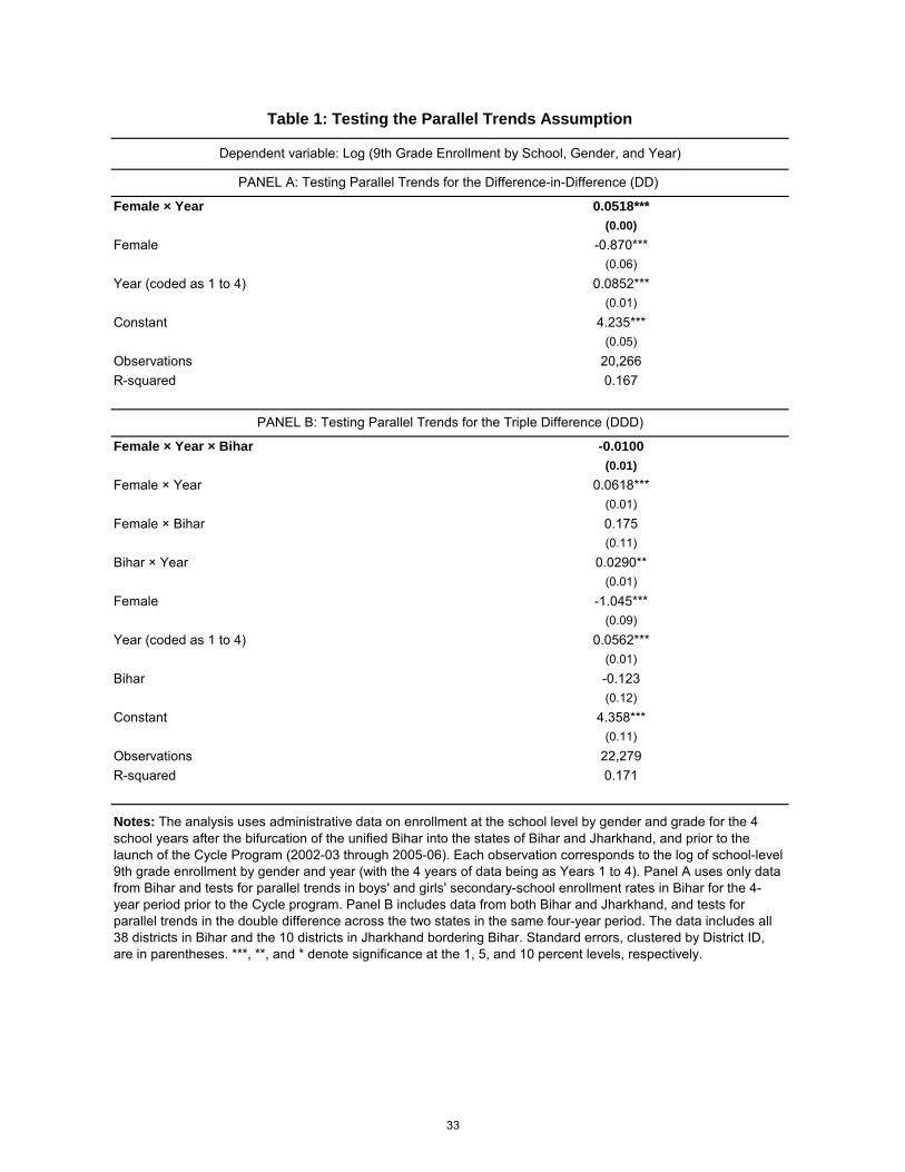
Female × Year 0.0518***

(0.00)

Female -0.870***(0.06)

Year (coded as 1 to 4) 0.0852***(0.01)

Constant 4.235***(0.05)

Observations 20,266R-squared 0.167

Female × Year × Bihar -0.0100

(0.01)

Female × Year 0.0618***(0.01)

Female × Bihar 0.175(0.11)

Bihar × Year 0.0290**(0.01)

Female -1.045***(0.09)

Year (coded as 1 to 4) 0.0562***(0.01)

Bihar -0.123(0.12)

Constant 4.358***(0.11)

Observations 22,279R-squared 0.171

Dependent variable: Log (9th Grade Enrollment by School, Gender, and Year)

PANEL A: Testing Parallel Trends for the Difference-in-Difference (DD)

PANEL B: Testing Parallel Trends for the Triple Difference (DDD)

Notes: The analysis uses administrative data on enrollment at the school level by gender and grade for the 4 school years after the bifurcation of the unified Bihar into the states of Bihar and Jharkhand, and prior to the launch of the Cycle Program (2002-03 through 2005-06). Each observation corresponds to the log of school-level 9th grade enrollment by gender and year (with the 4 years of data being as Years 1 to 4). Panel A uses only data from Bihar and tests for parallel trends in boys' and girls' secondary-school enrollment rates in Bihar for the 4-year period prior to the Cycle program. Panel B includes data from both Bihar and Jharkhand, and tests for parallel trends in the double difference across the two states in the same four-year period. The data includes all 38 districts in Bihar and the 10 districts in Jharkhand bordering Bihar. Standard errors, clustered by District ID, are in parentheses. ***, **, and * denote significance at the 1, 5, and 10 percent levels, respectively.

Table 1: Testing the Parallel Trends Assumption

33

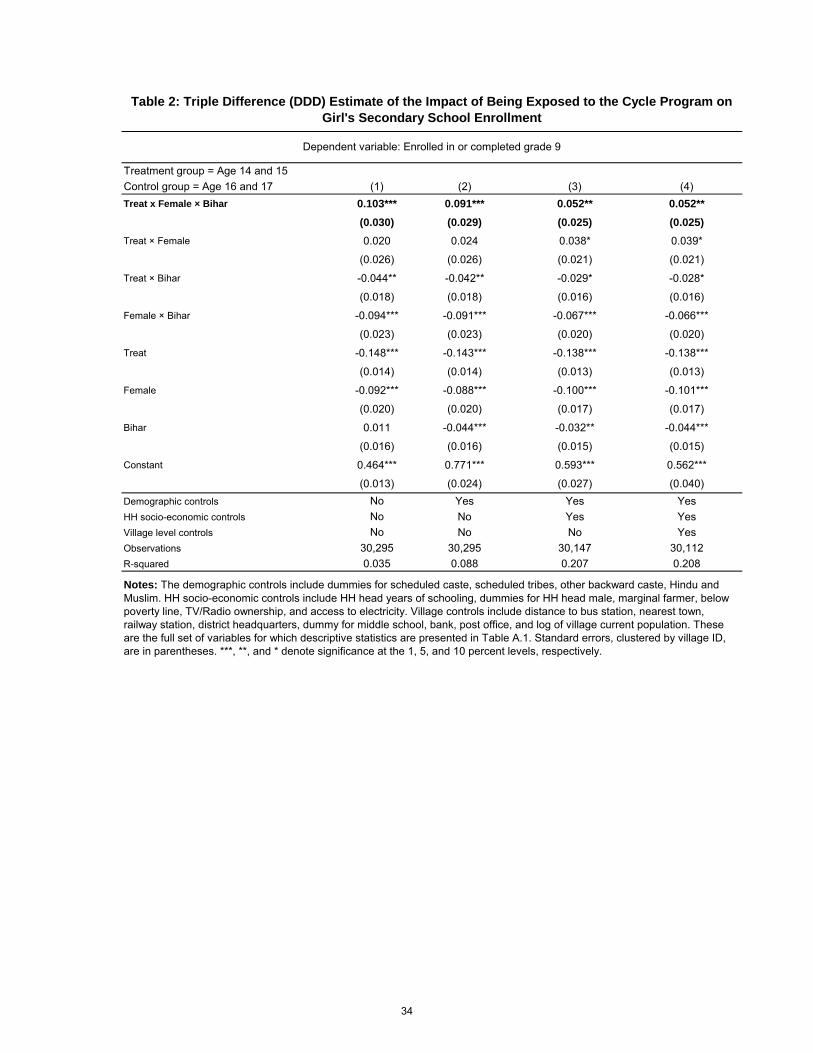
Treatment group = Age 14 and 15Control group = Age 16 and 17 (1) (2) (3) (4)Treat x Female × Bihar 0.103*** 0.091*** 0.052** 0.052**

(0.030) (0.029) (0.025) (0.025)

Treat × Female 0.020 0.024 0.038* 0.039*

(0.026) (0.026) (0.021) (0.021)

Treat × Bihar -0.044** -0.042** -0.029* -0.028*

(0.018) (0.018) (0.016) (0.016)

Female × Bihar -0.094*** -0.091*** -0.067*** -0.066***

(0.023) (0.023) (0.020) (0.020)

Treat -0.148*** -0.143*** -0.138*** -0.138***

(0.014) (0.014) (0.013) (0.013)

Female -0.092*** -0.088*** -0.100*** -0.101***

(0.020) (0.020) (0.017) (0.017)

Bihar 0.011 -0.044*** -0.032** -0.044***

(0.016) (0.016) (0.015) (0.015)

Constant 0.464*** 0.771*** 0.593*** 0.562***

(0.013) (0.024) (0.027) (0.040)Demographic controls No Yes Yes YesHH socio-economic controls No No Yes YesVillage level controls No No No YesObservations 30,295 30,295 30,147 30,112R-squared 0.035 0.088 0.207 0.208

Table 2: Triple Difference (DDD) Estimate of the Impact of Being Exposed to the Cycle Program on

Girl's Secondary School Enrollment

Notes: The demographic controls include dummies for scheduled caste, scheduled tribes, other backward caste, Hindu and Muslim. HH socio-economic controls include HH head years of schooling, dummies for HH head male, marginal farmer, below poverty line, TV/Radio ownership, and access to electricity. Village controls include distance to bus station, nearest town, railway station, district headquarters, dummy for middle school, bank, post office, and log of village current population. These are the full set of variables for which descriptive statistics are presented in Table A.1. Standard errors, clustered by village ID, are in parentheses. ***, **, and * denote significance at the 1, 5, and 10 percent levels, respectively.

Dependent variable: Enrolled in or completed grade 9

34

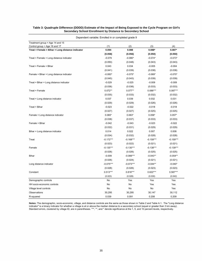
Treatment group = Age 14 and 15Control group = Age 16 and 17 (1) (2) (3) (4)Treat × Female × Bihar × Long distance indicator 0.094 0.088 0.088* 0.087*

(0.058) (0.056) (0.050) (0.050)

Treat × Female × Long distance indicator -0.079 -0.080* -0.074* -0.073*

(0.050) (0.048) (0.043) (0.043)

Treat × Female × Bihar 0.043 0.034 -0.005 -0.004

(0.041) (0.039) (0.038) (0.038)

Female × Bihar × Long distance indicator -0.083* -0.075* -0.069* -0.070*

(0.045) (0.043) (0.039) (0.039)

Treat × Bihar × Long distance indicator -0.029 -0.025 -0.009 -0.009

(0.036) (0.036) (0.033) (0.033)

Treat × Female 0.072** 0.077** 0.088*** 0.087***

(0.035) (0.033) (0.032) (0.032)

Treat × Long distance indicator 0.037 0.039 0.032 0.031

(0.029) (0.029) (0.026) (0.026)

Treat × Bihar -0.023 -0.022 -0.018 -0.018

(0.027) (0.027) (0.025) (0.025)

Female × Long distance indicator 0.065* 0.063* 0.058* 0.057*

(0.038) (0.037) (0.033) (0.033)

Female × Bihar -0.042 -0.043 -0.023 -0.022

(0.032) (0.031) (0.029) (0.029)

Bihar × Long distance indicator 0.014 0.022 0.007 0.008

(0.034) (0.032) (0.028) (0.028)

Treat -0.172*** -0.168*** -0.159*** -0.159***

(0.023) (0.022) (0.021) (0.021)

Female -0.135*** -0.130*** -0.138*** -0.139***

(0.028) (0.026) (0.025) (0.025)

Bihar -0.009 -0.066*** -0.043** -0.054**

(0.026) (0.024) (0.021) (0.021)

Long distance indicator -0.075*** -0.073*** -0.044** -0.040*

(0.028) (0.026) (0.023) (0.023)

Constant 0.513*** 0.816*** 0.622*** 0.587***

(0.023) (0.028) (0.030) (0.042)

Demographic controls No Yes Yes Yes

HH socio-economic controls No No Yes Yes

Village level controls No No No Yes

Observations 30,295 30,295 30,147 30,112

R-squared 0.039 0.091 0.208 0.209

Table 3: Quadruple Difference (DDDD) Estimate of the Impact of Being Exposed to the Cycle Program on Girl's

Secondary School Enrollment by Distance to Secondary School

Notes: The demographic, socio-economic, village, and distance controls are the same as those shown in Table 2 and Table A.1. The "Long distance indicator" is a binary indicator for whether a village is at or above the median distance to a secondary school (equal or greater than 3 km away). Standard errors, clustered by village ID, are in parentheses. ***, **, and * denote significance at the 1, 5, and 10 percent levels, respectively.

Dependent variable: Enrolled in or completed grade 9

35

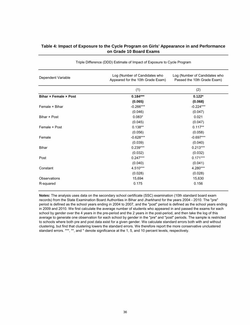
Dependent Variable Log (Number of Candidates who Appeared for the 10th Grade Exam)

Log (Number of Candidates who Passed the 10th Grade Exam)

(1) (2)

Bihar × Female × Post 0.184*** 0.122*

(0.065) (0.068)

Female × Bihar -0.266*** -0.224***(0.046) (0.047)

Bihar × Post 0.083* 0.021(0.045) (0.047)

Female × Post 0.138** 0.117**(0.056) (0.058)

Female -0.628*** -0.697***(0.039) (0.040)

Bihar 0.239*** 0.213***(0.032) (0.032)

Post 0.247*** 0.171***(0.040) (0.041)

Constant 4.510*** 4.280***(0.028) (0.028)

Observations 15,694 15,630R-squared 0.175 0.156

Table 4: Impact of Exposure to the Cycle Program on Girls' Appearance in and Performance

on Grade 10 Board Exams

Triple Difference (DDD) Estimate of Impact of Exposure to Cycle Program

Notes: The analysis uses data on the secondary school certificate (SSC) examination (10th standard board exam records) from the State Examination Board Authorities in Bihar and Jharkhand for the years 2004 - 2010. The "pre" period is defined as the school years ending in 2004 to 2007, and the "post" period is defined as the school years ending in 2009 and 2010. We first calculate the average number of students who appeared in and passed the exams for each school by gender over the 4 years in the pre-period and the 2 years in the post-period, and then take the log of this average to generate one observation for each school by gender in the "pre" and "post" periods. The sample is restricted to schools where both pre and post data exist for a given gender. We calculate standard errors both with and without clustering, but find that clustering lowers the standard errors. We therefore report the more conservative unclustered standard errors. ***, **, and * denote significance at the 1, 5, and 10 percent levels, respectively.

36

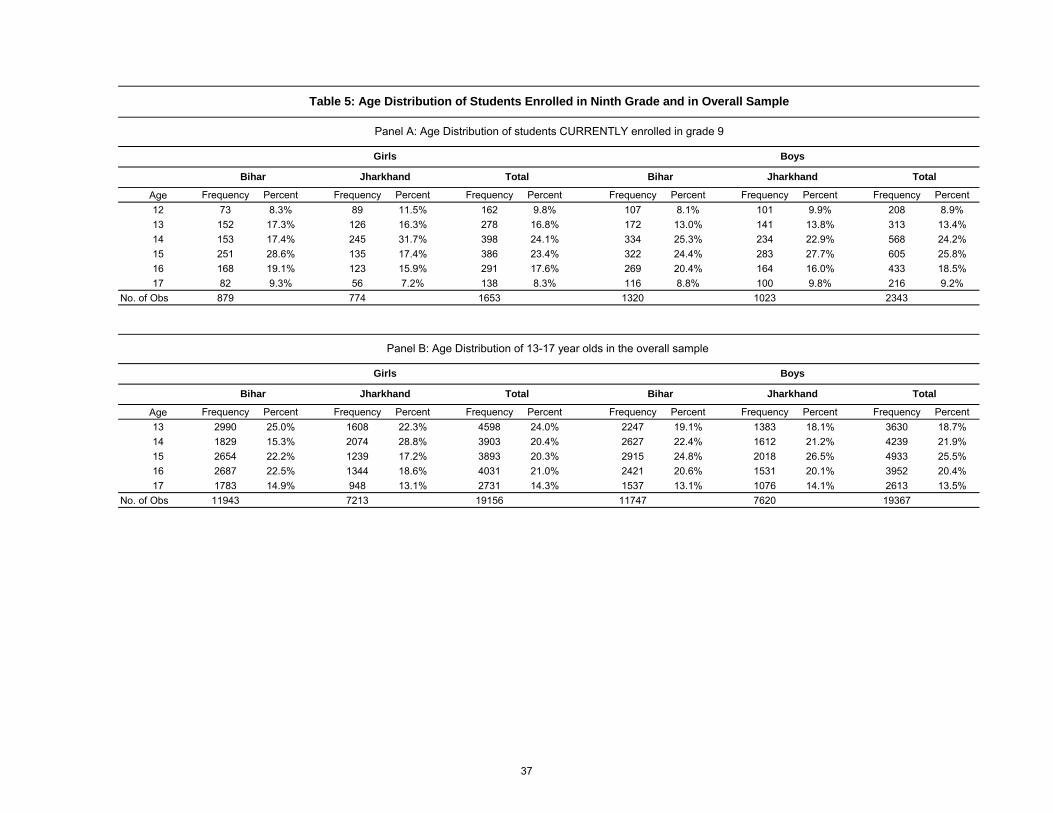
Age Frequency Percent Frequency Percent Frequency Percent Frequency Percent Frequency Percent Frequency Percent12 73 8.3% 89 11.5% 162 9.8% 107 8.1% 101 9.9% 208 8.9%13 152 17.3% 126 16.3% 278 16.8% 172 13.0% 141 13.8% 313 13.4%14 153 17.4% 245 31.7% 398 24.1% 334 25.3% 234 22.9% 568 24.2%15 251 28.6% 135 17.4% 386 23.4% 322 24.4% 283 27.7% 605 25.8%16 168 19.1% 123 15.9% 291 17.6% 269 20.4% 164 16.0% 433 18.5%17 82 9.3% 56 7.2% 138 8.3% 116 8.8% 100 9.8% 216 9.2%

No. of Obs 879 774 1653 1320 1023 2343

Age Frequency Percent Frequency Percent Frequency Percent Frequency Percent Frequency Percent Frequency Percent13 2990 25.0% 1608 22.3% 4598 24.0% 2247 19.1% 1383 18.1% 3630 18.7%14 1829 15.3% 2074 28.8% 3903 20.4% 2627 22.4% 1612 21.2% 4239 21.9%15 2654 22.2% 1239 17.2% 3893 20.3% 2915 24.8% 2018 26.5% 4933 25.5%16 2687 22.5% 1344 18.6% 4031 21.0% 2421 20.6% 1531 20.1% 3952 20.4%17 1783 14.9% 948 13.1% 2731 14.3% 1537 13.1% 1076 14.1% 2613 13.5%

No. of Obs 11943 7213 19156 11747 7620 19367

Table 5: Age Distribution of Students Enrolled in Ninth Grade and in Overall Sample

Girls Boys

Panel A: Age Distribution of students CURRENTLY enrolled in grade 9

Girls Boys

Panel B: Age Distribution of 13-17 year olds in the overall sample

Bihar Jharkhand Total Bihar Jharkhand Total

TotalBihar Jharkhand Total Bihar Jharkhand

37

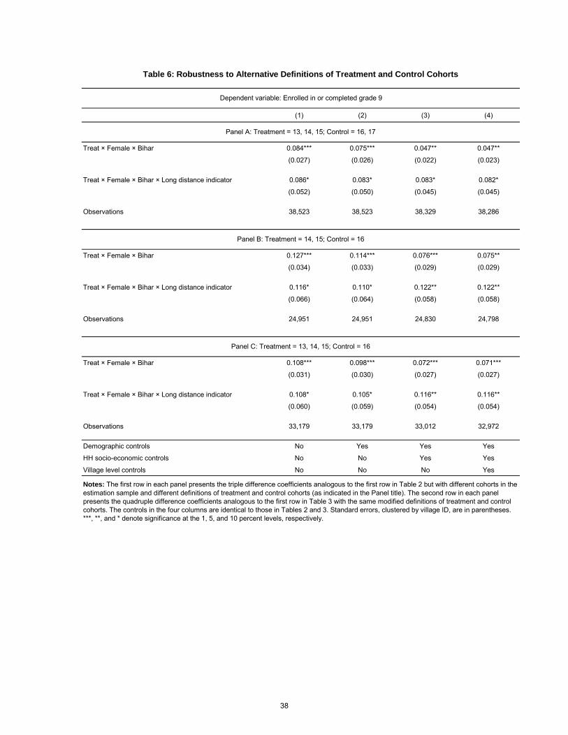
(1) (2) (3) (4)

Treat × Female × Bihar 0.084*** 0.075*** 0.047** 0.047**

(0.027) (0.026) (0.022) (0.023)

Treat × Female × Bihar × Long distance indicator 0.086* 0.083* 0.083* 0.082*

(0.052) (0.050) (0.045) (0.045)

Observations 38,523 38,523 38,329 38,286

Treat × Female × Bihar 0.127*** 0.114*** 0.076*** 0.075**

(0.034) (0.033) (0.029) (0.029)

Treat × Female × Bihar × Long distance indicator 0.116* 0.110* 0.122** 0.122**

(0.066) (0.064) (0.058) (0.058)

Observations 24,951 24,951 24,830 24,798

Treat × Female × Bihar 0.108*** 0.098*** 0.072*** 0.071***

(0.031) (0.030) (0.027) (0.027)

Treat × Female × Bihar × Long distance indicator 0.108* 0.105* 0.116** 0.116**

(0.060) (0.059) (0.054) (0.054)

Observations 33,179 33,179 33,012 32,972

Demographic controls No Yes Yes Yes

HH socio-economic controls No No Yes Yes

Village level controls No No No Yes

Notes: The first row in each panel presents the triple difference coefficients analogous to the first row in Table 2 but with different cohorts in the estimation sample and different definitions of treatment and control cohorts (as indicated in the Panel title). The second row in each panel presents the quadruple difference coefficients analogous to the first row in Table 3 with the same modified definitions of treatment and control cohorts. The controls in the four columns are identical to those in Tables 2 and 3. Standard errors, clustered by village ID, are in parentheses. ***, **, and * denote significance at the 1, 5, and 10 percent levels, respectively.

Table 6: Robustness to Alternative Definitions of Treatment and Control Cohorts

Panel A: Treatment = 13, 14, 15; Control = 16, 17

Panel B: Treatment = 14, 15; Control = 16

Panel C: Treatment = 13, 14, 15; Control = 16

Dependent variable: Enrolled in or completed grade 9

38

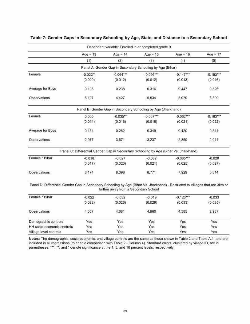
Age = 13 Age = 14 Age = 15 Age = 16 Age = 17

(1) (2) (3) (4) (5)

Female -0.022** -0.064*** -0.096*** -0.147*** -0.193***(0.009) (0.012) (0.012) (0.013) (0.016)

Average for Boys 0.105 0.238 0.316 0.447 0.526

Observations 5,197 4,427 5,534 5,070 3,300

Female 0.000 -0.035** -0.067*** -0.062*** -0.163***(0.014) (0.016) (0.018) (0.021) (0.022)

Average for Boys 0.134 0.262 0.349 0.420 0.544

Observations 2,977 3,671 3,237 2,859 2,014

Female * Bihar -0.018 -0.027 -0.032 -0.085*** -0.028(0.017) (0.020) (0.021) (0.025) (0.027)

Observations 8,174 8,098 8,771 7,929 5,314

Female * Bihar -0.022 -0.032 -0.019 -0.123*** -0.033(0.022) (0.026) (0.028) (0.033) (0.035)

Observations 4,557 4,681 4,960 4,385 2,987

Demographic controls Yes Yes Yes Yes YesHH socio-economic controls Yes Yes Yes Yes YesVillage level controls Yes Yes Yes Yes Yes

Notes: The demographic, socio-economic, and village controls are the same as those shown in Table 2 and Table A.1, and are included in all regressions (to enable comparison with Table 2 - Column 4). Standard errors, clustered by village ID, are in parentheses. ***, **, and * denote significance at the 1, 5, and 10 percent levels, respectively.

Table 7: Gender Gaps in Secondary Schooling by Age, State, and Distance to a Secondary School

Dependent variable: Enrolled in or completed grade 9

Panel A: Gender Gap in Secondary Schooling by Age (Bihar)

Panel B: Gender Gap in Secondary Schooling by Age (Jharkhand)

Panel C: Differential Gender Gap in Secondary Schooling by Age (Bihar Vs. Jharkhand)

Panel D: Differential Gender Gap in Secondary Schooling by Age (Bihar Vs. Jharkhand) - Restricted to Villages that are 3km or further away from a Secondary School

39

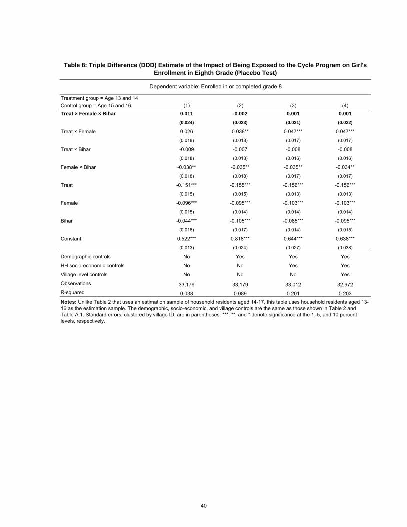
Treatment group = Age 13 and 14Control group = Age 15 and 16 (1) (2) (3) (4)Treat × Female × Bihar 0.011 -0.002 0.001 0.001

(0.024) (0.023) (0.021) (0.022)

Treat × Female 0.026 0.038** 0.047*** 0.047***

(0.018) (0.018) (0.017) (0.017)

Treat × Bihar -0.009 -0.007 -0.008 -0.008

(0.018) (0.018) (0.016) (0.016)

Female × Bihar -0.038** -0.035** -0.035** -0.034**

(0.018) (0.018) (0.017) (0.017)

Treat -0.151*** -0.155*** -0.156*** -0.156***

(0.015) (0.015) (0.013) (0.013)

Female -0.096*** -0.095*** -0.103*** -0.103***

(0.015) (0.014) (0.014) (0.014)

Bihar -0.044*** -0.105*** -0.085*** -0.095***

(0.016) (0.017) (0.014) (0.015)

Constant 0.522*** 0.818*** 0.644*** 0.638***

(0.013) (0.024) (0.027) (0.038)

Demographic controls No Yes Yes Yes

HH socio-economic controls No No Yes Yes

Village level controls No No No Yes

Observations 33,179 33,179 33,012 32,972R-squared 0.038 0.089 0.201 0.203

Table 8: Triple Difference (DDD) Estimate of the Impact of Being Exposed to the Cycle Program on Girl's

Enrollment in Eighth Grade (Placebo Test)

Notes: Unlike Table 2 that uses an estimation sample of household residents aged 14-17, this table uses household residents aged 13-16 as the estimation sample. The demographic, socio-economic, and village controls are the same as those shown in Table 2 and Table A.1. Standard errors, clustered by village ID, are in parentheses. ***, **, and * denote significance at the 1, 5, and 10 percent levels, respectively.

Dependent variable: Enrolled in or completed grade 8

40

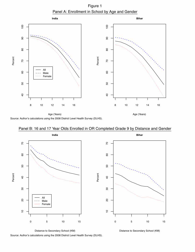
8 10 12 14 16

4050

6070

8090

100

Age (Years)

Perc

ent

India

AllMaleFemale

8 10 12 14 1640

5060

7080

9010

0

Age (Years)

Perc

ent

Bihar

0 5 10 15

1020

3040

5060

70

Distance to Secondary School (KM)

Perc

ent

India

AllMaleFemale

0 5 10 15

1020

3040

5060

70

Distance to Secondary School (KM)

Perc

ent

Bihar

Panel B: 16 and 17 Year Olds Enrolled in OR Completed Grade 9 by Distance and Gender

Panel A: Enrollment in School by Age and GenderFigure 1

Source: Author’s calculations using the 2008 District Level Health Survey (DLHS).

Source: Author’s calculations using the 2008 District Level Health Survey (DLHS).

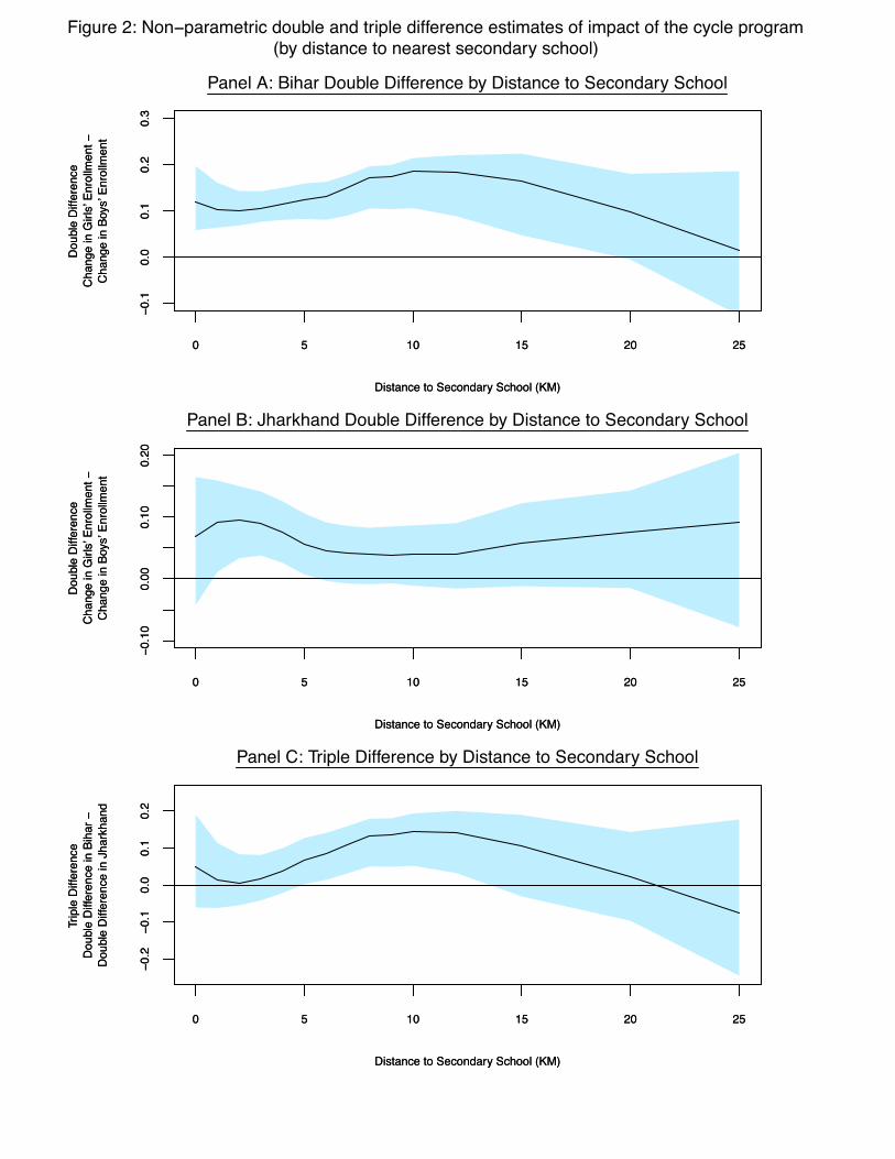
0 5 10 15 20 25

−0.1

0.0

0.1

0.2

0.3

Distance to Secondary School (KM)

Dou

ble

Diff

eren

ceC

hang

e in

Girl

s’ E

nrol

lmen

t −C

hang

e in

Boy

s’ E

nrol

lmen

tPanel A: Bihar Double Difference by Distance to Secondary School

0 5 10 15 20 25

−0.1

0.0

0.1

0.2

0.3

Distance to Secondary School (KM)

Dou

ble

Diff

eren

ceC

hang

e in

Girl

s’ E

nrol

lmen

t −C

hang

e in

Boy

s’ E

nrol

lmen

t

0 5 10 15 20 25

−0.1

00.

000.

100.

20

Distance to Secondary School (KM)

Dou

ble

Diff

eren

ceC

hang

e in

Girl

s’ E

nrol

lmen

t −C

hang

e in

Boy

s’ E

nrol

lmen

t

Panel B: Jharkhand Double Difference by Distance to Secondary School

0 5 10 15 20 25

−0.1

00.

000.

100.

20

Distance to Secondary School (KM)

Dou

ble

Diff

eren

ceC

hang

e in

Girl

s’ E

nrol

lmen

t −C

hang

e in

Boy

s’ E

nrol

lmen

t

0 5 10 15 20 25

−0.2

−0.1

0.0

0.1

0.2

Distance to Secondary School (KM)

Trip

le D

iffer

ence

Dou

ble

Diff

eren

ce in

Bih

ar −

Dou

ble

Diff

eren

ce in

Jha

rkha

nd

Panel C: Triple Difference by Distance to Secondary School

0 5 10 15 20 25

−0.2

−0.1

0.0

0.1

0.2

Distance to Secondary School (KM)

Trip

le D

iffer

ence

Dou

ble

Diff

eren

ce in

Bih

ar −

Dou

ble

Diff

eren

ce in

Jha

rkha

nd

Figure 2: Non−parametric double and triple difference estimates of impact of the cycle program(by distance to nearest secondary school)

 

 

For Online Publication Only 

“Cycling To School”: Appendix Tables and Figures 

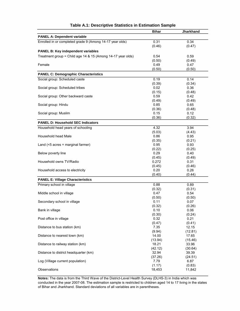
Bihar Jharkhand

PANEL A: Dependent variable

Enrolled in or completed grade 9 (Among 14-17 year olds) 0.31 0.34(0.46) (0.47)

PANEL B: Key independent variables

Treatment group = Child age 14 & 15 (Among 14-17 year olds) 0.54 0.59(0.50) (0.49)

Female 0.49 0.47(0.50) (0.50)

PANEL C: Demographic Characteristics

Social group: Scheduled caste 0.19 0.14(0.39) (0.34)

Social group: Scheduled tribes 0.02 0.36(0.15) (0.48)

Social group: Other backward caste 0.59 0.42(0.49) (0.49)

Social group: Hindu 0.85 0.65(0.36) (0.48)

Social group: Muslim 0.15 0.12(0.36) (0.32)

PANEL D: Household SEC Indicators

Household head years of schooling 4.32 3.94(5.03) (4.43)

Household head Male 0.86 0.95(0.35) (0.21)

Land (<5 acres = marginal farmer) 0.95 0.93(0.22) (0.25)

Below poverty line 0.29 0.40(0.45) (0.49)

Household owns TV/Radio 0.272 0.31(0.45) (0.46)

Household access to electricity 0.20 0.26(0.40) (0.44)

PANEL E: Village Characteristics

Primary school in village 0.88 0.89(0.32) (0.31)

Middle school in village 0.47 0.54(0.50) (0.50)

Secondary school in village 0.11 0.07(0.32) (0.26)

Bank in village 0.10 0.06(0.30) (0.24)

Post office in village 0.32 0.21(0.47) (0.41)

Distance to bus station (km) 7.35 12.15(9.94) (12.81)

Distance to nearest town (km) 14.00 17.65(13.94) (15.46)

Distance to railway station (km) 18.21 33.96(42.12) (30.64)

Distance to district headquarter (km) 32.94 39.39(37.26) (24.51)

Log (Village current population) 7.79 6.87(1.17) (0.83)

Observations 18,453 11,842

Table A.1: Descriptive Statistics in Estimation Sample

Notes: The data is from the Third Wave of the District-Level Health Survey (DLHS-3) in India which was conducted in the year 2007-08. The estimation sample is restricted to children aged 14 to 17 living in the states of Bihar and Jharkhand. Standard deviations of all variables are in parentheses.

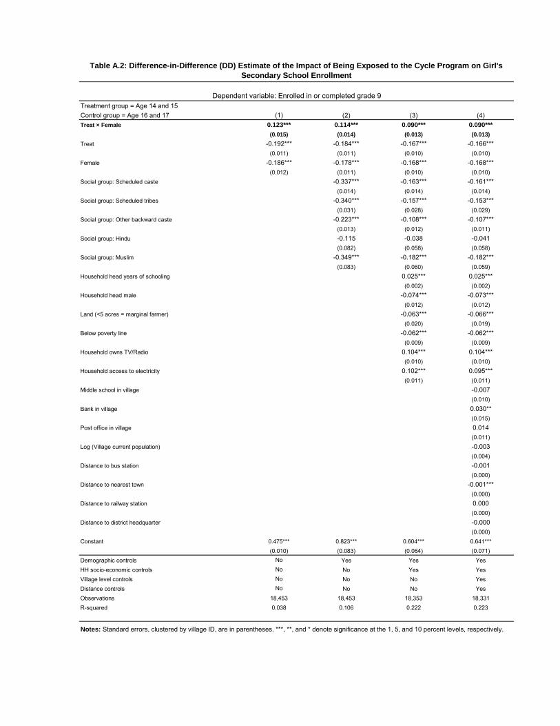
Treatment group = Age 14 and 15Control group = Age 16 and 17 (1) (2) (3) (4)Treat × Female 0.123*** 0.114*** 0.090*** 0.090***

(0.015) (0.014) (0.013) (0.013)

Treat -0.192*** -0.184*** -0.167*** -0.166***(0.011) (0.011) (0.010) (0.010)

Female -0.186*** -0.178*** -0.168*** -0.168***(0.012) (0.011) (0.010) (0.010)

Social group: Scheduled caste -0.337*** -0.163*** -0.161***(0.014) (0.014) (0.014)

Social group: Scheduled tribes -0.340*** -0.157*** -0.153***(0.031) (0.028) (0.029)

Social group: Other backward caste -0.223*** -0.108*** -0.107***(0.013) (0.012) (0.011)

Social group: Hindu -0.115 -0.038 -0.041(0.082) (0.058) (0.058)

Social group: Muslim -0.349*** -0.182*** -0.182***(0.083) (0.060) (0.059)

Household head years of schooling 0.025*** 0.025***(0.002) (0.002)

Household head male -0.074*** -0.073***(0.012) (0.012)

Land (<5 acres = marginal farmer) -0.063*** -0.066***(0.020) (0.019)

Below poverty line -0.062*** -0.062***(0.009) (0.009)

Household owns TV/Radio 0.104*** 0.104***(0.010) (0.010)

Household access to electricity 0.102*** 0.095***(0.011) (0.011)

Middle school in village -0.007(0.010)

Bank in village 0.030**(0.015)

Post office in village 0.014(0.011)

Log (Village current population) -0.003(0.004)

Distance to bus station -0.001(0.000)

Distance to nearest town -0.001***(0.000)

Distance to railway station 0.000(0.000)

Distance to district headquarter -0.000(0.000)

Constant 0.475*** 0.823*** 0.604*** 0.641***(0.010) (0.083) (0.064) (0.071)

Demographic controls No Yes Yes YesHH socio-economic controls No No Yes YesVillage level controls No No No YesDistance controls No No No YesObservations 18,453 18,453 18,353 18,331R-squared 0.038 0.106 0.222 0.223

Notes: Standard errors, clustered by village ID, are in parentheses. ***, **, and * denote significance at the 1, 5, and 10 percent levels, respectively.

Table A.2: Difference-in-Difference (DD) Estimate of the Impact of Being Exposed to the Cycle Program on Girl's

Secondary School Enrollment

Dependent variable: Enrolled in or completed grade 9

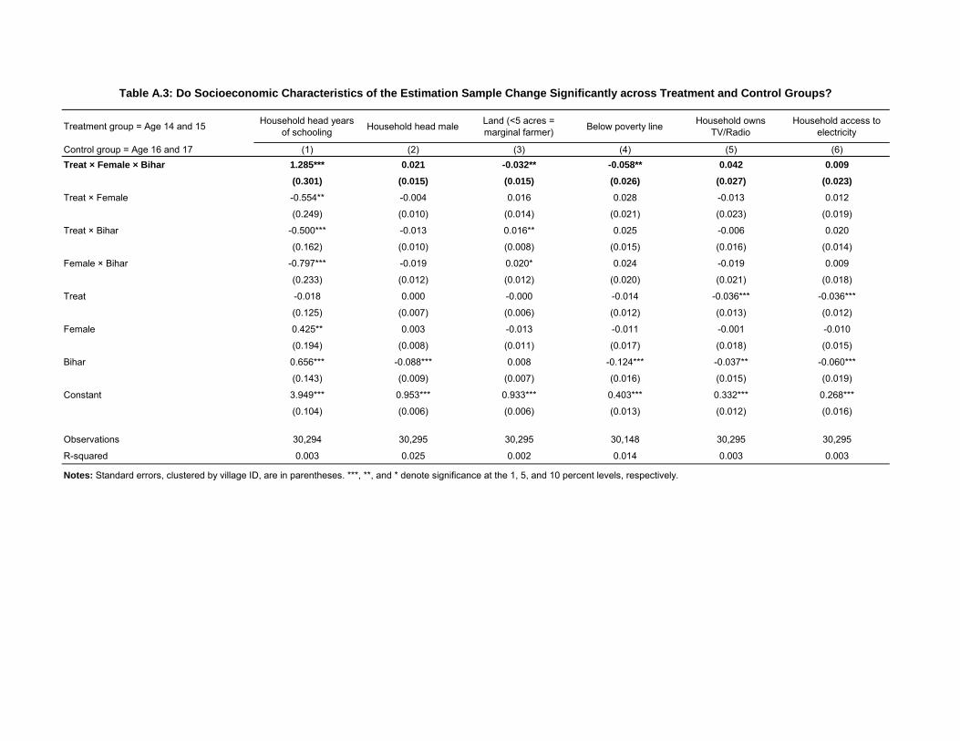
Treatment group = Age 14 and 15 Household head years of schooling Household head male Land (<5 acres =

marginal farmer) Below poverty line Household owns TV/Radio

Household access to electricity

Control group = Age 16 and 17 (1) (2) (3) (4) (5) (6)Treat × Female × Bihar 1.285*** 0.021 -0.032** -0.058** 0.042 0.009

(0.301) (0.015) (0.015) (0.026) (0.027) (0.023)

Treat × Female -0.554** -0.004 0.016 0.028 -0.013 0.012

(0.249) (0.010) (0.014) (0.021) (0.023) (0.019)

Treat × Bihar -0.500*** -0.013 0.016** 0.025 -0.006 0.020

(0.162) (0.010) (0.008) (0.015) (0.016) (0.014)

Female × Bihar -0.797*** -0.019 0.020* 0.024 -0.019 0.009

(0.233) (0.012) (0.012) (0.020) (0.021) (0.018)

Treat -0.018 0.000 -0.000 -0.014 -0.036*** -0.036***

(0.125) (0.007) (0.006) (0.012) (0.013) (0.012)

Female 0.425** 0.003 -0.013 -0.011 -0.001 -0.010

(0.194) (0.008) (0.011) (0.017) (0.018) (0.015)

Bihar 0.656*** -0.088*** 0.008 -0.124*** -0.037** -0.060***

(0.143) (0.009) (0.007) (0.016) (0.015) (0.019)

Constant 3.949*** 0.953*** 0.933*** 0.403*** 0.332*** 0.268***

(0.104) (0.006) (0.006) (0.013) (0.012) (0.016)

Observations 30,294 30,295 30,295 30,148 30,295 30,295

R-squared 0.003 0.025 0.002 0.014 0.003 0.003

Table A.3: Do Socioeconomic Characteristics of the Estimation Sample Change Significantly across Treatment and Control Groups?

Notes: Standard errors, clustered by village ID, are in parentheses. ***, **, and * denote significance at the 1, 5, and 10 percent levels, respectively.

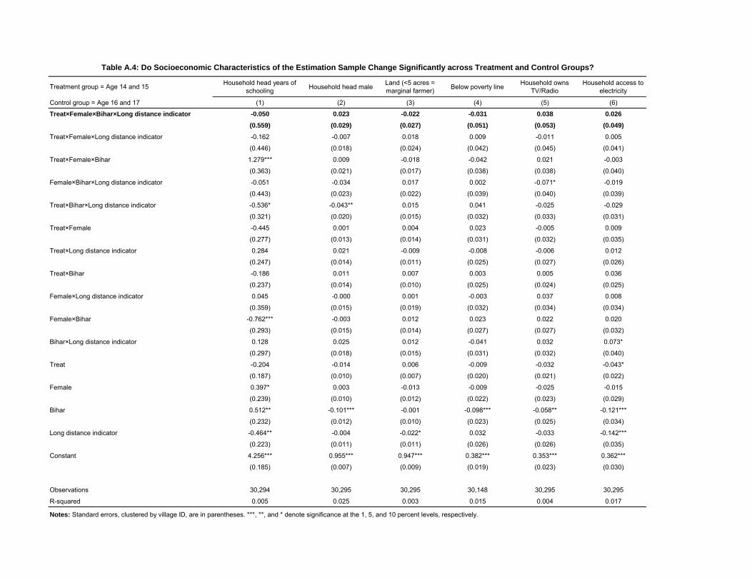
Treatment group = Age 14 and 15 Household head years of schooling Household head male Land (<5 acres =

marginal farmer) Below poverty line Household owns TV/Radio

Household access to electricity

Control group = Age 16 and 17 (1) (2) (3) (4) (5) (6)

Treat×Female×Bihar×Long distance indicator -0.050 0.023 -0.022 -0.031 0.038 0.026

(0.559) (0.029) (0.027) (0.051) (0.053) (0.049)

Treat×Female×Long distance indicator -0.162 -0.007 0.018 0.009 -0.011 0.005

(0.446) (0.018) (0.024) (0.042) (0.045) (0.041)

Treat×Female×Bihar 1.279*** 0.009 -0.018 -0.042 0.021 -0.003

(0.363) (0.021) (0.017) (0.038) (0.038) (0.040)

Female×Bihar×Long distance indicator -0.051 -0.034 0.017 0.002 -0.071* -0.019

(0.443) (0.023) (0.022) (0.039) (0.040) (0.039)

Treat×Bihar×Long distance indicator -0.536* -0.043** 0.015 0.041 -0.025 -0.029

(0.321) (0.020) (0.015) (0.032) (0.033) (0.031)

Treat×Female -0.445 0.001 0.004 0.023 -0.005 0.009

(0.277) (0.013) (0.014) (0.031) (0.032) (0.035)

Treat×Long distance indicator 0.284 0.021 -0.009 -0.008 -0.006 0.012

(0.247) (0.014) (0.011) (0.025) (0.027) (0.026)

Treat×Bihar -0.186 0.011 0.007 0.003 0.005 0.036

(0.237) (0.014) (0.010) (0.025) (0.024) (0.025)

Female×Long distance indicator 0.045 -0.000 0.001 -0.003 0.037 0.008

(0.359) (0.015) (0.019) (0.032) (0.034) (0.034)

Female×Bihar -0.762*** -0.003 0.012 0.023 0.022 0.020

(0.293) (0.015) (0.014) (0.027) (0.027) (0.032)

Bihar×Long distance indicator 0.128 0.025 0.012 -0.041 0.032 0.073*

(0.297) (0.018) (0.015) (0.031) (0.032) (0.040)

Treat -0.204 -0.014 0.006 -0.009 -0.032 -0.043*

(0.187) (0.010) (0.007) (0.020) (0.021) (0.022)

Female 0.397* 0.003 -0.013 -0.009 -0.025 -0.015

(0.239) (0.010) (0.012) (0.022) (0.023) (0.029)

Bihar 0.512** -0.101*** -0.001 -0.098*** -0.058** -0.121***

(0.232) (0.012) (0.010) (0.023) (0.025) (0.034)

Long distance indicator -0.464** -0.004 -0.022* 0.032 -0.033 -0.142***

(0.223) (0.011) (0.011) (0.026) (0.026) (0.035)

Constant 4.256*** 0.955*** 0.947*** 0.382*** 0.353*** 0.362***

(0.185) (0.007) (0.009) (0.019) (0.023) (0.030)

Observations 30,294 30,295 30,295 30,148 30,295 30,295

R-squared 0.005 0.025 0.003 0.015 0.004 0.017

Table A.4: Do Socioeconomic Characteristics of the Estimation Sample Change Significantly across Treatment and Control Groups?

Notes: Standard errors, clustered by village ID, are in parentheses. ***, **, and * denote significance at the 1, 5, and 10 percent levels, respectively.

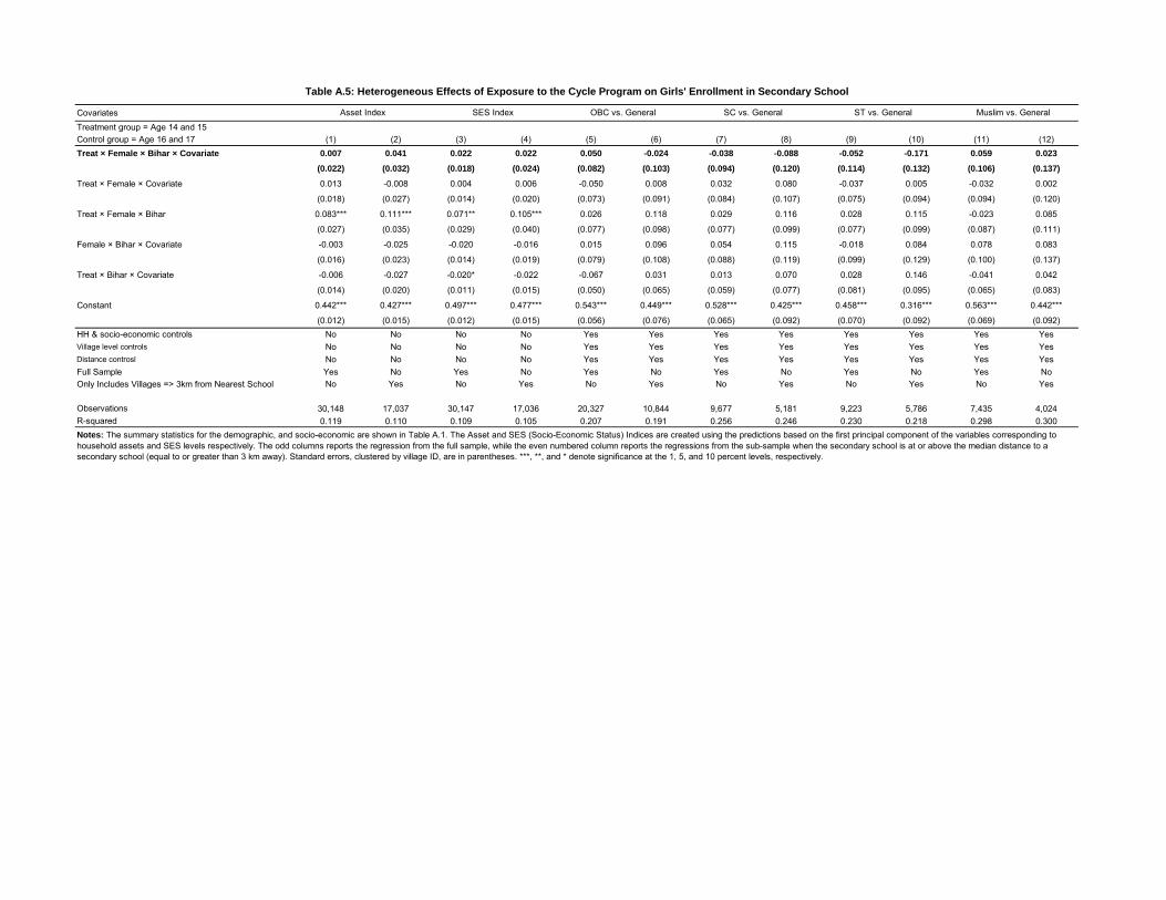
CovariatesTreatment group = Age 14 and 15Control group = Age 16 and 17 (1) (2) (3) (4) (5) (6) (7) (8) (9) (10) (11) (12)Treat × Female × Bihar × Covariate 0.007 0.041 0.022 0.022 0.050 -0.024 -0.038 -0.088 -0.052 -0.171 0.059 0.023

(0.022) (0.032) (0.018) (0.024) (0.082) (0.103) (0.094) (0.120) (0.114) (0.132) (0.106) (0.137)

Treat × Female × Covariate 0.013 -0.008 0.004 0.006 -0.050 0.008 0.032 0.080 -0.037 0.005 -0.032 0.002

(0.018) (0.027) (0.014) (0.020) (0.073) (0.091) (0.084) (0.107) (0.075) (0.094) (0.094) (0.120)

Treat × Female × Bihar 0.083*** 0.111*** 0.071** 0.105*** 0.026 0.118 0.029 0.116 0.028 0.115 -0.023 0.085

(0.027) (0.035) (0.029) (0.040) (0.077) (0.098) (0.077) (0.099) (0.077) (0.099) (0.087) (0.111)

Female × Bihar × Covariate -0.003 -0.025 -0.020 -0.016 0.015 0.096 0.054 0.115 -0.018 0.084 0.078 0.083

(0.016) (0.023) (0.014) (0.019) (0.079) (0.108) (0.088) (0.119) (0.099) (0.129) (0.100) (0.137)

Treat × Bihar × Covariate -0.006 -0.027 -0.020* -0.022 -0.067 0.031 0.013 0.070 0.028 0.146 -0.041 0.042

(0.014) (0.020) (0.011) (0.015) (0.050) (0.065) (0.059) (0.077) (0.081) (0.095) (0.065) (0.083)

Constant 0.442*** 0.427*** 0.497*** 0.477*** 0.543*** 0.449*** 0.528*** 0.425*** 0.458*** 0.316*** 0.563*** 0.442***

(0.012) (0.015) (0.012) (0.015) (0.056) (0.076) (0.065) (0.092) (0.070) (0.092) (0.069) (0.092)HH & socio-economic controls No No No No Yes Yes Yes Yes Yes Yes Yes YesVillage level controls No No No No Yes Yes Yes Yes Yes Yes Yes YesDistance controsl No No No No Yes Yes Yes Yes Yes Yes Yes YesFull Sample Yes No Yes No Yes No Yes No Yes No Yes NoOnly Includes Villages => 3km from Nearest School No Yes No Yes No Yes No Yes No Yes No Yes

Observations 30,148 17,037 30,147 17,036 20,327 10,844 9,677 5,181 9,223 5,786 7,435 4,024R-squared 0.119 0.110 0.109 0.105 0.207 0.191 0.256 0.246 0.230 0.218 0.298 0.300Notes: The summary statistics for the demographic, and socio-economic are shown in Table A.1. The Asset and SES (Socio-Economic Status) Indices are created using the predictions based on the first principal component of the variables corresponding to household assets and SES levels respectively. The odd columns reports the regression from the full sample, while the even numbered column reports the regressions from the sub-sample when the secondary school is at or above the median distance to a secondary school (equal to or greater than 3 km away). Standard errors, clustered by village ID, are in parentheses. ***, **, and * denote significance at the 1, 5, and 10 percent levels, respectively.

Table A.5: Heterogeneous Effects of Exposure to the Cycle Program on Girls' Enrollment in Secondary School

Asset Index SES Index OBC vs. General SC vs. General ST vs. General Muslim vs. General

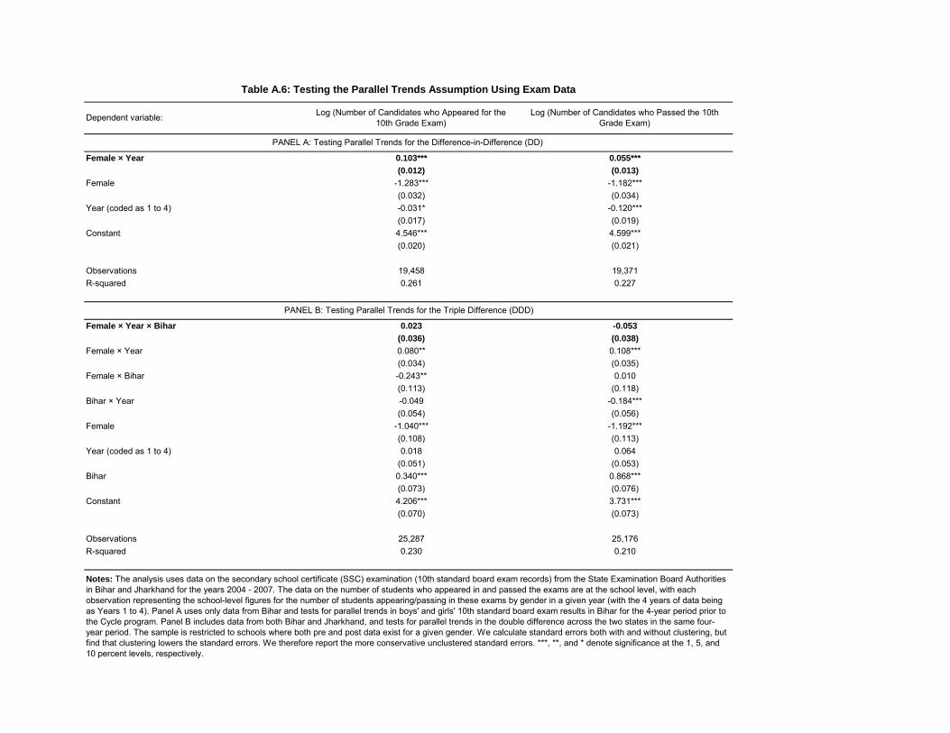
Female × Year 0.103*** 0.055***

(0.012) (0.013)

Female -1.283*** -1.182***(0.032) (0.034)

Year (coded as 1 to 4) -0.031* -0.120***(0.017) (0.019)

Constant 4.546*** 4.599***(0.020) (0.021)

Observations 19,458 19,371R-squared 0.261 0.227

Female × Year × Bihar 0.023 -0.053

(0.036) (0.038)

Female × Year 0.080** 0.108***(0.034) (0.035)

Female × Bihar -0.243** 0.010(0.113) (0.118)

Bihar × Year -0.049 -0.184***(0.054) (0.056)

Female -1.040*** -1.192***(0.108) (0.113)

Year (coded as 1 to 4) 0.018 0.064(0.051) (0.053)

Bihar 0.340*** 0.868***(0.073) (0.076)

Constant 4.206*** 3.731***(0.070) (0.073)

Observations 25,287 25,176R-squared 0.230 0.210

Notes: The analysis uses data on the secondary school certificate (SSC) examination (10th standard board exam records) from the State Examination Board Authorities in Bihar and Jharkhand for the years 2004 - 2007. The data on the number of students who appeared in and passed the exams are at the school level, with each observation representing the school-level figures for the number of students appearing/passing in these exams by gender in a given year (with the 4 years of data being as Years 1 to 4). Panel A uses only data from Bihar and tests for parallel trends in boys' and girls' 10th standard board exam results in Bihar for the 4-year period prior to the Cycle program. Panel B includes data from both Bihar and Jharkhand, and tests for parallel trends in the double difference across the two states in the same four-year period. The sample is restricted to schools where both pre and post data exist for a given gender. We calculate standard errors both with and without clustering, but find that clustering lowers the standard errors. We therefore report the more conservative unclustered standard errors. ***, **, and * denote significance at the 1, 5, and 10 percent levels, respectively.

Log (Number of Candidates who Passed the 10th Grade Exam)

PANEL A: Testing Parallel Trends for the Difference-in-Difference (DD)

PANEL B: Testing Parallel Trends for the Triple Difference (DDD)

Table A.6: Testing the Parallel Trends Assumption Using Exam Data

Dependent variable: Log (Number of Candidates who Appeared for the 10th Grade Exam)

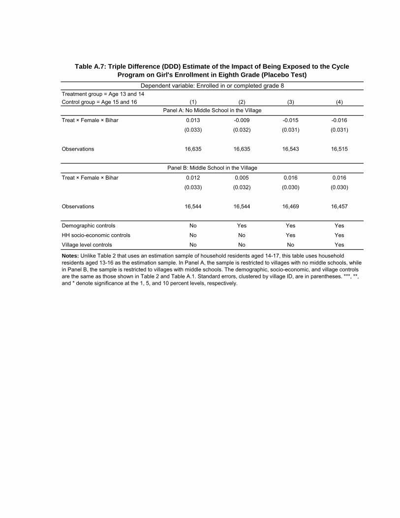
Treatment group = Age 13 and 14Control group = Age 15 and 16 (1) (2) (3) (4)

Treat × Female × Bihar 0.013 -0.009 -0.015 -0.016

(0.033) (0.032) (0.031) (0.031)

Observations 16,635 16,635 16,543 16,515

Treat × Female × Bihar 0.012 0.005 0.016 0.016

(0.033) (0.032) (0.030) (0.030)

Observations 16,544 16,544 16,469 16,457

Demographic controls No Yes Yes Yes

HH socio-economic controls No No Yes Yes

Village level controls No No No Yes

Notes: Unlike Table 2 that uses an estimation sample of household residents aged 14-17, this table uses household residents aged 13-16 as the estimation sample. In Panel A, the sample is restricted to villages with no middle schools, while in Panel B, the sample is restricted to villages with middle schools. The demographic, socio-economic, and village controls are the same as those shown in Table 2 and Table A.1. Standard errors, clustered by village ID, are in parentheses. ***, **, and * denote significance at the 1, 5, and 10 percent levels, respectively.

Table A.7: Triple Difference (DDD) Estimate of the Impact of Being Exposed to the Cycle

Program on Girl's Enrollment in Eighth Grade (Placebo Test)

Dependent variable: Enrolled in or completed grade 8

Panel A: No Middle School in the Village

Panel B: Middle School in the Village

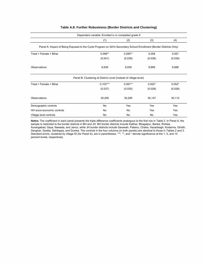
(1) (2) (3) (4)

Treat × Female × Bihar 0.099** 0.095** 0.058 0.057

(0.041) (0.039) (0.036) (0.036)

Observations 9,939 9,939 9,899 9,886

Treat × Female × Bihar 0.103*** 0.091** 0.052* 0.052*

(0.037) (0.035) (0.028) (0.028)

Observations 30,295 30,295 30,147 30,112

Demographic controls No Yes Yes Yes

HH socio-economic controls No No Yes Yes

Village level controls No No No Yes

Table A.8: Further Robustness (Border Districts and Clustering)

Panel A: Impact of Being Exposed to the Cycle Program on Girl's Secondary School Enrollment (Border Districts Only)

Panel B: Clustering at District Level (instead of village-level)

Dependent variable: Enrolled in or completed grade 9

Notes: The coefficient in each panel presents the triple difference coefficients analogous to the first row in Table 2. In Panel A, the sample is restricted to the border districts in BH and JH. BH border districts include Katihar, Bhagalpur, Banka, Rohtas, Aurangabad, Gaya, Nawada, and Jamui, while JH border districts include Garawah, Palamu, Chatra, Hazaribagh, Kodarma, Giridih, Deoghar, Godda, Sahibganj, and Dumka. The controls in the four columns (in both panels) are identical to those in Tables 2 and 3. Standard errors, clustered by village ID (for Panel A), are in parentheses. ***, **, and * denote significance at the 1, 5, and 10 percent levels, respectively.

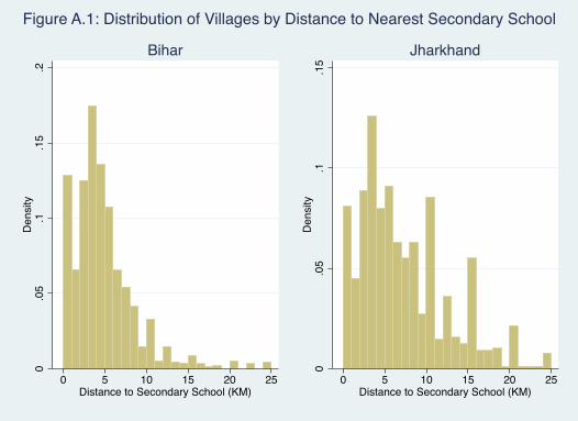
0.0

5.1

.15

.2D

ensi

ty

0 5 10 15 20 25Distance to Secondary School (KM)

Bihar

0.0

5.1

.15

Den

sity

0 5 10 15 20 25Distance to Secondary School (KM)

Jharkhand

Figure A.1: Distribution of Villages by Distance to Nearest Secondary School

 

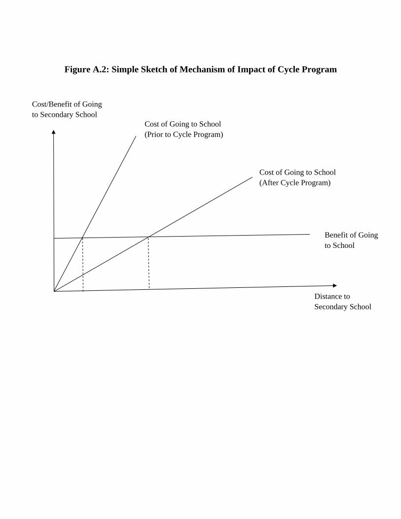
Figure A.2: Simple Sketch of Mechanism of Impact of Cycle Program

 

 

 

Distance to Secondary School

Cost/Benefit of Going to Secondary School

Benefit of Going to School

Cost of Going to School (Prior to Cycle Program)

Cost of Going to School (After Cycle Program)