Cycling chaos: its creation, persistence and loss of stability in a model of nonlinear magnetoconvection

ELSEVIER Physica D 122 (1998) 134-154

PHY$1CA

Cycling chaos: its creation, persistence and loss of stability in a model of nonlinear magnetoconvection

Peter Ashwin a, A.M. Rucklidge b,, a Department of Mathematical and Computing Sciences, University of Surrey, Guildford GU2 5XH, UK

b Department of Applied Mathematics and Theoretical Physics, University of Cambridge, Silver Street, Cambridge CB3 9EW, UK

Received 15 October 1997; received in revised form 12 February 1998; accepted 17 March 1998 Communicated by A.C. Newell

Abstract

We examine a model system where attractors may consist of a heteroclinic cycle between chaotic sets; this 'cycling chaos' manifests itself as trajectories that spend increasingly long periods lingering near chaotic invariant sets interspersed with short transitions between neighbourhoods of these sets. Such behaviour is robust to perturbations that preserve the symmetry of the system; we examine bifurcations of this state.

We discuss a scenario where an attracting cycling chaotic state is created at a blowout bifurcation of a chaotic attractor in an invariant subspace. This differs from the standard scenario for the blowout bifurcation in that in our case, the blowout is neither subcritical nor supercritical. The robust cycling chaotic state can be followed to a point where it loses stability at a resonance bifurcation and creates a series of large period attractors.

The model we consider is a ninth-order truncated ordinary differential equation (ODE) model of three-dimensional incompressible convection in a plane layer of conducting fluid subjected to a vertical magnetic field and a vertical temperature gradient. Symmetries of the model lead to the existence of invariant subspaces for the dynamics; in particular there are invariant subspaces that correspond to regimes of two-dimensional flows, with variation in the vertical but only one of the two horizontal directions. Stable two-dimensional chaotic flow can go unstable to three-dimensional flow via the cross-roll instability: We show how the bifurcations mentioned above can be located by examination of various transverse Liapunov exponents. We also consider a reduction of the ODE to a map and demonstrate that the same behaviour can be found in the corresponding map. This allows us to describe and predict a number of observed transitions in these models. The dynamics we describe is new but nonetheless robust, and so should occur in other applications. © 1998 Elsevier Science B.V.

PACS: 05.45+; 47.20.Ky; 47.65 Keywords: Heteroclinic cycle; Symmetry; Chaotic dynamics; Magnetoconvection

* Corresponding author. E-mail: [email protected].

0167-2789/98/$19.00 © 1998 Elsevier Science B.V. All rights reserved PH S0167-2789(98)00174-2

P. Ashwin, A.M. Rucklidge/Physica D 122 (1998) 134-154 135

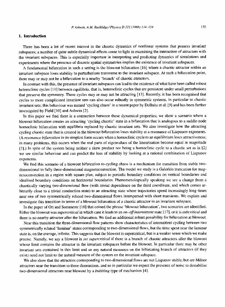
1. Introduction

There has been a lot of recent interest in the chaotic dynamics of nonlinear systems that possess invariant

subspaces; a number of quite subtle dynamical effects come to light in examining the interaction of attractors with

the invariant subspaces. This is especially important in interpreting and predicting dynamics of simulations and

experiments where the presence of discrete spatial symmetries implies the existence of invariant subspaces.

A fundamental bifurcation in such a setting is the blowout bifurcation [16] where a chaotic attractor within an

invariant subspace loses stability to perturbations transverse to the invariant subspace. At such a bifurcation point,

there may or may not be a bifurcation to a nearby 'branch' of chaotic attractors.

In contrast with this, the presence of invariant subspaces can lead to the existence of what have been called robust

heteroclinic cycles [ 11 ] between equilibria, that is, heteroclinic cycles that are persistent under small perturbations

that preserve the symmetry. These cycles may or may not be attracting [13]. Recently, it has been recognised that

cycles to more complicated invariant sets can also occur robustly in symmetric systems, in particular to chaotic

invariant sets; this behaviour was named 'cycling chaos' in a recent paper by Dellnitz et al. [9] and has been further

investigated by Field [10] and Ashwin [2]. In this paper we find there is a connection between these dynamical properties; we show a scenario where a

blowout bifurcation creates an attracting 'cycling chaotic' state in a bifurcation that is analogous to a saddle-node

homoclinic bifurcation with equilibria replaced by chaotic invafiant sets. We also investigate how the attracting

cycling chaotic state that is created in the blowout bifurcation loses stability at a resonance of Liapunov exponents.

(A resonance bifurcation in its simplest form occurs when a homoclinic cycle to an equilibrium loses attractiveness;

in many problems, this occurs when the real parts of eigenvalues of the linearisation become equal in magnitude

[7].) In spite of the system being neither a skew product nor being a homoclinic cycle to a chaotic set as in [2]

we see similar behaviour and can predict the loss of stability by looking at a rational combination of Liapunov

exponents. We find this scenario of a blowout bifurcation to cycling chaos is a mechanism for transition from stable two-

dimensional to fully three-dimensional magnetoconvection. The model we study is a Galerkin truncation for mag-

netoconvection in a region with square plan, subject to periodic boundary conditions on vertical boundaries and

idealised boundary conditions on horizontal boundaries. Phenomenologically speaking we see a change from a

chaotically varying two-dimensional flow (with trivial dependence on the third coordinate, and which comes ar-

bitrarily close to a trivial conduction state) to an attracting state where trajectories spend increasingly long times

near one of two symmetrically related two-dimensional flows interspersed with short transients. We explain and

investigate this transition in terms of a blowout bifurcation of a chaotic attractor in an invariant subspace.

In the paper of Ott and Sommerer [ 16] that coined the phrase 'blowout bifurcation', two scenarios are identified.

Either the blowout was supercritical in which case it leads to an on-offintermittent state [ 17], or it is subcritical and

there is no nearby attractor after the bifurcation. We find an additional robust possibility for bifurcation at blowout.

Near this transition the three-dimensional flow patterns show characteristics of intermittent cycling between two

symmetrically related 'laminar' states corresponding to two-dimensional flows, but the time spent near the laminar

state is, on the average, infinite. This suggests that the blowout is supercritical, but in a weaker sense which we make

precise. Namely, we say a blowout is set supercritical if there is a branch of chaotic attractors after the blowout

whose limit contains the attractor in the invariant subspaces before the blowout. In particular there may be other

invariant sets contained in this limit and so any natural measures on the bifurcating branch of attractors (if they

exist) need not limit to the natural measure of the system on the invariant subspace. We also show that the attractors corresponding to two-dimensional flows are not Liapunov stable, but are Milnor

attractors near the transition to three dimensions, and so in particular we expect the presence of noise to destabilise

two-dimensional attractors near blowout by a bubbling type of mechanism [4].

136 P. Ashwin, A.M. Rucklidge / Physica D 122 (1998) 134-154

We find in our example that the state of cycling chaos is attracting once it has been created: trajectories cycle between neighbourhoods of the chaotic sets within the invariant subspaces, and the time between switches from one neighbourhood to the next increases geometrically as trajectories get closer and closer to the invariant subspaces.

By estimating the rate of increase of switching times, we are able to show that cycling chaos ceases to be attracting in a resonance bifurcation. One remarkable aspect of this study is that we are able to predict the parameter values at

which the blowout bifurcation and the resonance occur, requiring only a single numerical average over the chaotic set within the invariant subspace.

Our approach to this problem is a combination of careful numerical simulations and analysis of problems with the symmetry of the model to gain insight into the dynamics. By reducing to an approximate map, we can perform fast and accurate long-time simulations and hence get a fuller picture of the dynamics and bifurcations that determine the behaviour in this model.

The paper is organised as follows: in Section 2 we introduce the ODE model for magnetoconvection, discuss

its symmetries and corresponding invariant subspaces. We also summarise what is known about the dynamics of

the ODE model. This is followed by a description of the creation, persistence and loss of stability of the cycling chaos on varying a parameter in numerical simulations in Section 3. Section 4 shows how one can, under certain assumptions, derive a map model of the dynamics of the ODE that has the same dynamical behaviour. Section 5 is a

theoretical analysis of the blowout bifurcation that creates the cycling chaotic attractor and is followed in Section 6 by a theoretical analysis of its loss of stability. Finally, Section 7 discusses some of the implications of this work on the chaotic dynamics of symmetric systems.

2. An ODE model for magnetoconvection

The model we study is an ODE on ~9 described by the following equations:

3¢0 = IZXo "~- Xo0 -- X2Xl - - / 3 y 2 x o , Xl = --VXl + xox2, :t2 = - t rx2 -- tr Qa + yxoxl,

yo = Izyo + yoO - y2yt - / 3 x ~ y o , yl = - v y l + yoy2, y2 = - t r y 2 - tr Qb + Y y o y l , (1)

t~ = ((x2 - a), b = ((y2 - b), 0 = - 0 - x 2 - y02.

These ODEs have been derived as an asymptotic limit of a model of three-dimensional incompressible convection in a plane layer, with an imposed vertical magnetic field; for further details and details of its derivation, see [14,19,20].

In the context of this model, x0 and Y0 represent the amplitudes of convective rolls with their axes aligned in the Y and X (horizontal) directions, respectively, Xl and yl represent modes that cause the rolls to tilt, and x2 and Y2 represent shear across the layer in the X and Y directions. The modes a and b represent the horizontal component of the magnetic field in the X and Y directions, and 0 represents the horizontally averaged temperature.

The model has five primary parameters: # is proportional to the imposed temperature difference across the layer,

with/z = 0 at the initial bifurcation to convection; 13 is related to the horizontal spatial periodicity length, but is an arbitrary small parameter in the model of [14,19]; tr and ( are dimensionless viscous and magnetic diffusion coefficients; and Q is proportional to the square of the imposed magnetic field. Note that tr, ( and Q are scaled by factors of 4, 4 and zr 2 from their usage in [ 14,19,20]. Two secondary parameters that we use are y = 3 ( 1 + 4a) / 16tr and v = (9tr/(1 + 4tr)) - / z . In the parameter regime of interest, all parameters are non-negative.

2.1. Symmetr ies o f the model

Consider D4ArT 2 acting on the plane with unit cell [0, 2Yr) 2 in the usual way, with the toms T 2 acting by translations on the plane, and D4 by reflections in the axes and rotation through zr/2. We define the following group

P. Ashwin, A.M. Rucklidge / Physica D 122 (1998) 134-154 137

elements

Kx : i

I ( x :

K y : I Ky :

p :

r(~,n) :

reflection through X = 0,

reflection through X = rr/2,

reflection through Y = 0,

reflection through Y = zc/2,

re/2 rotation about (X, Y) = (Jr, zr),

translation,

(X, Y) ~ ( - X , Y),

(X, Y) w-~ (~r - X, Y),

(x, r ) ~ ( x , - r ) , (X, Y) ~ (X, Jr - Y),

(X, Y) w-~ (27r - Y, X),

( X , Y ) ~ ( X + ~ , Y + r / ) .

Note that p, r(~,o) and any reflection Jc can be used to generate the group D 4 + T 2.

We consider the subgroup

a = (Kx, KIx, Ky, KtV, p).

(2)

(3)

Since G contains the subgroup (7/2) 2, generated by rxX' x and KyKy, of translations T e, it follows that G is isomorphic

to a semidirect product Dn~(Ze) 2 (IGI = 32). The ODE (1) is equivariant under the group G of symmetries acting on R 9 by

Xx(XO, Xl, x2, Yo, Yl, Y2, a, b, O) = (xo, - X l , - x 2 , Yo, Yl, Y2, - a , b, 0),

x'(xo, Xl, x2, Yo, Yl, Y2, a, b, O) = ( - x o , Xl, - x 2 , Yo, Yl, Y2, - a , b, 0), (4)

p(xo, x], x2, Yo, Yl, Y2, a, b, 0) = (Yo, - Y l , -Y2, xo, x l , x2, - b , a, 0).

This action gives rise to a number of isotropy types, shown in Table 1. Fig. 1 gives a partial isotropy lattice for

this group action. Dynamics in F always decays to the trivial equilibrium point, corresponding to the absence of

convection. We refer to dynamics in Px and Py as two-dimensional, since these correspond to two-dimensional

convection in the original problem (though dim Px is 5). Dynamics in Rx and Ry corresponds to mirror symmetric

two-dimensional rolls, with their axes aligned along the Y and X directions; we refer to equilibrium points in these

subspaces as x-rol ls and y-rolls, respectively. In Px and Py, convection is two-dimensional but not mirror symmetric,

and is referred to as tilted rolls. Dynamics in Qx and Qy corresponds to three-dimensional convection that is still

invariant under one mirror reflection (tilted rolls with a cross-roll component). Otherwise we say the dynamics is

fully three-dimensional.

In a slight break from convention we say the fixed point subspaces S as having isotropy subgroup Iso(S) rather

than considering the isotropy subgroups as the fundamental objects.

Table 1 Selected fixed point subspaces S of the action of G o n R 9 together with name, representative point and dimension of S

S Name Representative point dim S

F Full symmetry (0, 0, 0, 0, 0, 0, 0, 0, t) 1 Rx x-Rolls (x, 0, 0, 0, 0, 0, 0, 0, t) 2 Ry y-Rolls (0, 0, 0, x, 0, 0, 0, 0, t) 2 D+ + Diagonal (x, 0, 0, x, 0, 0, 0, 0, t) 2 D_ - Diagonal (x, 0, 0, - x , 0, 0, 0, 0, t) 2 Rxy Mixed modes (x, 0, 0, y, 0, 0, 0, 0, t) 3 Px x-Rolls + shear (x, y, z, 0, 0, 0, a, 0, t) 5 Pv y-Rolls + shear (0, 0, 0, x, y, z, 0, a, t) 5 Qx x-Rolls + shear + crossrolls (x, y, z, w, 0, 0, a, 0, t) 6 Qy y-Rolls + shear + crossrolls (w, 0, 0, x, y, z, 0, a, t) 6 T No symmetry (u, o, w, x, y, z, a, b, t) 9

There are others (e.g. (0, x, 0, 0, 0, 0, 0, 0, t)) but these are not important for the dynamics we discuss here.

138 P. Ashwin, A.M. Rucklidge/Physica D 122 (1998) 134-154

F

Rx By D+ D_

P~ Py R~y

COx C2y \ /

T

Fig. 1. A portion of the isotropy lattice for the action of G on N 9 under which (1) is equivariant. We have shown fixed point subspaces of some conjugate subgroups separately for clarity. The isotropies of Px and Pv are the smallest isotropies that physically involve only two-dimensional effects.

2.2. Summary of known dynamics of the model

There has been a great deal of work already on analysing the dynamics of some special cases of the model (1). Rucklidge and Matthews [20] considered two-dimensional convection (that is, restricted to Px) and conducted a detailed survey of the resulting PDEs and the fifth-order set of ODEs, focussing on two parameter regimes: first the non-magnetic case (with Q = 0, and/z and tr varying) and then the magnetic case (with tr = 0.125 and ( = 0.05, with/z and Q varying). For small but non-zero values of Q (for example, Q = 1/rr2), the typical pattern

of behaviour that they found was: the rolls created in the initial convective instability at /z = 0 lose stability to

tilted rolls at # = 0.04324, which in turn undergo a Hopf bifurcation at/z = 0.13696. There is then a complicated sequence of global bifurcations involving the collision of periodic orbits with the trivial and roll equilibrium points.

Amongst these numerous bifurcations, there is a parameter interval (0.16544 < /_t < 0.16566) with Lorenz- like chaotic dynamics. A detailed comparison with simulations of the PDEs for two-dimensional incompressible magnetoconvection confirmed the qualitative similarity between the dynamics of the PDEs and of the ODEs.

This approach was extended to three-dimensional convection [14] and magnetoconvection [19]. With the parameters fixed at Q = 1/zr 2, tr = 0.125, ~ = 0.05 and/3 = 0.5, Rucklidge and Matthews [19] found that as/z is increased, there is an instability from two-dimensional tilted rolls in Px to three-dimensional convection in Qx at /z = 0.06305, before the Hopf bifurcation in Px. The three-dimensional steady solutions undergo a Hopf bifurcation at /z = 0.07807. The resulting periodic orbit, which is contained in Qx, undergoes a series of period-doubling bifurcations leading to chaos, but by/z = 0.09, all that remains is an attracting structurally stable heteroclinic cycle

connecting four equilibrium points (in Rx, Px, Ry and Pv). This cycle ceases to be attracting a t /z = 0.09514 (computed using a method adopted from [13]). The value of/z at which the heteroclinic cycle ceases to be attracting increases with/3, and for/3 > 1.2, the Hopf bifurcation from tilted rolls occurs in Px before the heteroclinic cycle loses stability, suggesting that there will be an attracting heteroclinic cycle connecting two roll equilibrium points in Rx and Ry and two periodic orbits in Px and Py. Numerical evidence in both the ODE model and in the PDEs for compressible convection indicates that this is indeed the case [14]. Since the periodic orbit in Px is known to become chaotic for higher/z, Matthews et al. [14] speculated that there might be an attracting heteroclinic cycle

connecting the chaotic sets in Px and Py.


In this paper, we address issues raised by this earlier work: if there is a heteroclinic cycle connecting chaotic sets in these ODEs, how is it created, exactly in what way are the connections structurally stable, and how can

its asymptotic stability be computed? We choose/z = 0.1655 (with the other parameters as in [20]) so that the dynamics within pr is chaotic, and vary 13, which does not alter the dynamics in Px but does affect how the chaotic set within Px responds to perturbations outside that subspace. We dicuss only the dynamics of the ODEs, not the PDEs, but note that in the earlier studies, the ODEs have modelled the behaviour of the PDEs remarkably

well.

3. Numerical simulations of the ODEs

We present numerical simulations of the ODEs that demonstrate two aspects of cycling chaos that we seek

to explain: how cycling chaos can be created in a blowout bifurcation, and how cycling chaos can cease to be

attracting. We concentrate on parameter values that are known to have Lorenz-like chaotic dynamics within p~- and P,,:

/z = 0.1655, Q = 1/rr 2, cr = 0.125, ~" = 0.05 (5)

(and hence v = 0.5845 and y = 2.25), although we note that qualitatively similar attractors are found for a large proportion of nearby parameter values. These parameter values correspond to those in Figs. 15(c) and 20(a) in [20]. The numerical method used was a Bulirsch-Stoer adaptive integrator [ 18], with a tolerance for the relative error set to 10 -12 for each step.

We use the parameter fl as a normal parameter (see [5]) for the dynamics in Px and P,,; that is, it con- trois instabilities transverse to Px and Pv in the directions Qx and Qy without altering the dynamics inside p,.

or P,,.

3.1. Cycling chaos

In Fig. 2 we show a typical example of timeseries when there is attracting cycling chaos (with fl = 2.0). The system starts with x0 oscillating chaotically while Y0 is quiescent, switches to a state where Y0 oscillates chaotically while x0 is quiescent, and so on. A more careful examination reveals that after a switch the trajectory remains close to a fixed point in Rx o r Ry for an increasing length of time. Physically, this corresponds to chaotic two-dimensional convection that switches between rolls aligned in the X and Y directions. Fig. 2(c) shows the chaotic trajectories

projected onto the (x0, x2) plane, while (d) illustrates switching between Px (the 'horizontal' plane) and Pv (the 'vertical' plane).

Note how the chaotic behaviour in Figs. 2(a) and (b) repeats: trajectories spend longer and longer near the unstable manifolds of the x-roll and y-roll equilibrium points and take longer and longer between each switch. This is illustrated further in Fig. 3, which shows intersections of a trajectory with the Poincar6 surface Ix21 + [y21 = 0.01 close to the trivial solution. There are two phases evident in the cycle: the order one chaotic behaviour of x0

near p~ (while Y0 grows exponentially), and the exponential growth of Ix01 as the trajectory moves away from Pv (while y0 behaves chaotically). The time between switches increases monotonically and the rate of increase varies with ¢~, the normal parameter. In these numerical simulations, the switching time saturates when certain components of the solution come close to the machine accuracy of the computations (about 10 -323 for double precision).

We argue that this is evidence for attracting cycling chaos: trajectories approach a structurally stable heteroclinic cycle between chaotic sets. In Fig. 4 we show a schematic picture of the heteroclinic cycle. We recall that the fixed


0.4

0.2

0.0

-0.2

-0.4

0

(a) • . j , , . . . , . . . , r . •

J i i i

2000 4000 6000 8000 10000 t

0.4

0.2

0.0

-0.2

-0.4

0

0.4

0.2

0.0

-0.2

-0.4

(b) • • . i . • • i . • . , • r , . . .

2000 4000 6000 8000

(c)

. i . i , . , i , , t . . , i .

-0.4 -0.2 0.0 0.2 0.4 Xo

1 0 0 0 0

t

Fig. 2. Numerical solutions of the model ODEs with/z = 0.1655, Q = 1/Jr 2, tr = 0.125, ( = 0.05 and fl = 2.0. (a) x0 against time; (b) Y0 against time; (c) x0 against x2; (d) x0, Y0 and Ix2[ + ly2l in perspective. The crosses in (c) and (d) represent the x-roll, y-roll and trivial equilibrium points in Rx, Ry and F. Note that the chaotic attractor is close to a heteroclinic cycle that connects the x-rolls, the y-rolls and the trivial fixed point.

po in t spaces Rx and Ry are two-dimens ional , gxy is three-dimensional , Px and Py are f ive-dimensional and Qx and Qy are s ix-d imens ional invariant subspaces in the n ine-d imens iona l phase space. The sys tem starts near the x- ro l l

equ i l ib r ium point in Rx, which is unstable to shear (x2); the parameters are such that the unstable mani fo ld o f x- ro l l s

comes c lose to the trivial solut ion and returns to a ne ighbourhood of x-rol ls . This g lobal near-connect ion within Px

is the source o f the chaot ic behaviour. We refer to the chaotic sets in Px and Py as Ax and Ay, respect ively; these

P Ashwin, A.M. Rucklidge/Physica D 122 (1998) 134-154 141

100 t * ~ 1 0 - 1 0 ~ "

lo-2O _ i 10_30 [ i

0

(a) ~+'7-+"-'b~

i

8.104 1.105 2.10 4 4 .10 4 6 .10 4 t

100[ . . . . . . . . . :~-,~ . . ~ ,

1 0 - 2 0 ~ :: :

1 0 - 3 0 / 0 2"104 "4 , i0 4 '

(b) : ~.--? ,~:~. .~

& i O 4 t

8 . i 0 4 1.10 5

(c) 1001 . . . . . . . . . . ~ . * * . ~ .~ . , . . ~ .~ .~,- ~-- . ~ .~,, • ..... : ,

__ l o - l O ' : : i ' : : : : : ! ! " . : i :

lo-2O i l i i ; ! i 1 0 - 3 0 [ ' i i ! : : : ; . : /

~ , ¢ . . • . - : ~ .

0 2"10 4 4"10 4 6"10 4 8"10 4 1"10 5 t

(d) 100~:i~?:'~:~:*:~7~:'~: ~" :~ :':.i~ ~ ~ :~ :~" ;~" :~ :~" :~ :'~" ~-i :~-. .~- : ~

"~ 1 0 - 2 0 [ - : : : i i : !: " !: ! !: ! :' i i 1 0 - 3 0 [ : .: !. i . i. ! .! :. i. i i .: ,i ; .:' i ,! .

0 2"10 4 4"10 4 6"10 4 8"10 4 1"10 5 t

Fig. 3. Numerical solutions of the model ODEs: cycling chaos with (a) fl = 2.00, (b) fl = 1.80, (c) fl = 1.65 and (d) fl = 1.63, showing the values of Ix01 at which the trajectory intersects the surface defined by Ix21 + lY21 = 0.01. The rising exponential growth phases correspond to the system switching from chaos in Py to chaos in Ix. The time between switches increases as the system approaches the attracting cycling chaos, but the rate of increase depends on ft.

contain the relevant roll equi l ibr ium points and they both contain the trivial solution, so there are structurally stable

connect ions f rom the trivial solution to the roll equi l ibr ium points and f rom those to Ax and Ay. Within Qx, Ax is unstable to cross-rol ls (Y0) since the trivial solution is equal ly unstable in the x0 and Y0 directions. Eventually, Y0 grows large enough that there is a switch to the y-rol l equi l ibr ium point in Ry, at which point y2 starts to grow. Thus

the cycle connects invariant sets in the fol lowing fixed point subspaces:

• "" ~ Rx -"+ Px ~ Qx ~ Ry ~ Py --+ Qy --+ . . . (6)

be tween the equi l ibr ium points in Rx and Ry, and Ax and Ay within Px and Py, with the structurally stable connect ions needed to comple te the cycle f rom Ax and Ay to the y-rol l and x-rol l equi l ibr ium points lying within

Qx and Qy.


p

..... Qy Qy

Fig. 4. A schematic illustration of the location of the robust cycle relative to the invariant subspaces forced by symmetry. The cycle is between the chaotic invariant sets Ax and Ay (within Px and Py) and two fixed points contained in Rx and Ry. The cycle is robust to G-equivariant perturbations that fix the dynamics in Px and Py. The intersection of Px and Py at the trivial solution is not shown, although Ax and Ay do in fact intersect there.

Note that our scenario is certainly a simplification of the full set of heteroclinic connections; there are other fixed points contained in the closure of the smallest attracting invariant set, in particular the origin is contained within the cycle.

3.2. Blowout

We turn now to the question of how the cycling chaos is created. With/3 = 3.5 we find attracting two-dimensional

chaos (Figs. 5(a) and (b)), which loses stability around/3 = 3.47 (c) in a blowout bifurcation, and for/3 = 3.40 (d),

there is exponential growth away from Px into Qx. Within Qx, the y-roll equilibrium points are sinks, establishing the structurally stable connection from the chaos in Px to the equilibrium point in Ry, and hence the creation of cycling chaos.

3.3. Resonance

As illustrated in Fig. 3, as/3 decreases towards 1.63, trajectories spend progressively longer in each visit to Px and Py before switching to the conjugate chaotic invariant set. Eventually, trajectories come arbitrarily close to the invariant subspaces Px and Py (limited only by machine accuracy in the numerical simulations). Fig. 6 shows

how the time intervals between switches between Ax and Ay increases as the system approaches this heteroclinic cycle, and how the rate of approach to the heteroclinic cycle decreases as/3 approaches 1.62. The intervals between

switches grow by a factor of about 1.4, 1.2 and 1.1 per switch for/3 = 2.00,/3 = 1.80 and/3 = 1.65 respectively, and 1.03 and 1.02 for/3 = 1.64 and 1.63. By/3 ~ 1.62, the heteroclinic cycle is no longer attracting, and for /3 = 1.61 and 1.60, the system settles down to periodic behaviour that is bounded away from Px and Py, though the periodic orbits are actually quite close to these invariant subspaces. For these calculations, we imposed a cut-off of 10-1°°: the calculation ceased once any variable became smaller than this.

In the next section, we derive a map that allows us to compute longer trajectories more accurately, and we demonstrate cycling chaos, its creation in a blowout bifurcation and its loss of attractiveness using this map. We analyse the blowout bifurcation in Section 5, and argue in Section 6 that the cycling chaos created in that bifurcation ceases to be attractive at a resonance.


(a) 0.6 0.4 0.2 0.0

-0.2 -0.4 -0.6

0 1000 2000 3000 4000 5000

(b) 10-15 . . . . . . . . . . . . .

10-20i~-, . . . . . . . -A~A-, . ~ .- . . . .

1o_25 10-30

0 1000 2000 3000 4000 5000 t

(c) 1o-15 L . . . . . . .

10-20 ; ]

--~ 10_25

10-30

0 1000 2000 3000 4000 5000 t

(d) 10-15.

_ 10 -20

,o-25 NVVWVVVVVVVVVVVVVV , , , , , , , ,, ,, . . . . - -

10 -30

0 1000 2000 3000 4000 5000 t

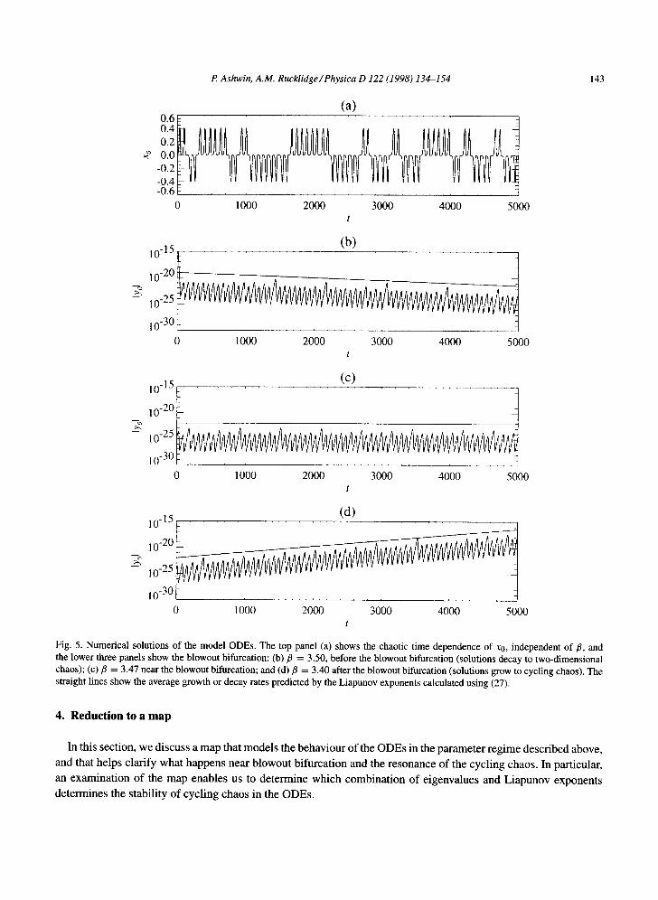
Fig. 5. Numerical solutions of the model ODEs. The top panel (a) shows the chaotic time dependence of x0, independent of t , and the lower three panels show the blowout bifurcation: (b) fl = 3.50, before the blowout bifurcation (solutions decay to two-dimensional chaos); (c) fl = 3.47 near the blowout bifurcation; and (d) fl = 3.40 after the blowout bifurcation (solutions grow to cycling chaos). The straight lines show the average growth or decay rates predicted by the Liapunov exponents calculated using (27).

4. R e d u c t i o n to a m a p

In this section, we discuss a map that models the behaviour of the ODEs in the parameter regime described above,

and that helps clarify what happens near blowout bifurcation and the resonance of the cycling chaos. In particular,

an examination of the map enables us to determine which combination of eigenvalues and Liapunov exponents determines the stability of cycling chaos in the ODEs.


.=_

4000

3000

2000

1000

. . . . . . . . . I . . . . . . . . . I . . . . . . . . .

[3 = 1.64, 1.63

e~t

f [3 = 1.62

[3= 1.61

13 = 1.60

, i i i i , i i i [ , J i i , i i ~ i I i , , , i i i , ,

0 100 200 300 switch

Fig. 6. Time intervals between switches between Px and Py with/~ in the range 1.60-1.64. The intervals between switches increase by a factor of about 1.03 and 1.02 per switch for/~ = 1.64 and 1.63, respectively. The switching times stop increasing once the values of variables become so small that the cubic terms in the ODEs cannot be represented accurately with double-precision numbers (and calculations were terminated once any variable went below 10-1°°). For fl = 1.61 and 1.60, the system approaches a periodic orbit and the intervals between switches go to a constant (though in the case of fl = 1.61, the periodic orbit is only achieved after 1500 switches).

4.1. Derivation

We rely on a map derived for the two-dimensional dynamics by breaking up the flow into pieces near and

between equilibrium points [20]. Within the Px subspace, the leading stable eigendirection of the origin (that is,

the eigendirection with negative eigenvalue closest to zero) is in the (xe, a) plane, and the unstable direction of

the origin is along the x0 axis. All trajectories leaving the origin in that direction follow the structurally stable

connection within Rx to one or other of the x-roll equilibrium points. The one-dimensional unstable manifold of

x-rolls lies within Px, and the chaotic attractor is associated with a global bifurcation at which that unstable manifold

collides with the origin. Near this global bifurcation, the dynamics within Px is modelled by an augmented Lorenz

map:

(xo, x2 = =El) ~-+ ( sgn(xo) ( -x + C11xol~), - x e ) (7)

defined as a map from the surface of section Ix2[ = h to itself. Details of the derivation are given in [20], but

briefly, t¢ is a parameter related to / z in the ODEs, with x = 0 at the global bifurcation; h is a small positive

constant that we scale to one; sgn(x) = +1 if x > 0 and - 1 if x < 0; 81 depends on the ratio of various stable

and unstable eigenvalues at the origin and the x-roll equilibrium points (with 0 < 81 < 1); and C1 is a (negative)

constant. It is a straightforward matter to include the effect of a small perturbation in the y0 and Y2 directions. Near the Px

subspace, Yo and Y2 will grow linearly at a rate that depends on xo. This means that we get a mapping of the form

(xo, x2 = q-l, Yo, Y2) ~-~ ( sgn(x0) ( -x + C1 Ix0181), - x 2 , C2yolxo[ ~2, CayElxol~3), (8)

where C2 and Ca are constants and the exponents 82 and 83 again depend on ratios of eigenvalues, with 82 < 0 and 83 > 0. The exponent 82 is negative since a small value of x0 implies that the trajectory spends longer near the

P Ashwin, A.M. Rucklidge/Physica D 122 (1998) 134-154 145

origin, so YO has a longer time to grow. Similarly, near Py we get the mapping

(xo, x2, YO, Y2 = -4-1) ~ (CexolYo182, C3x2lYo183, s g n ( y o ) ( - x + CI lYol 8~), - y e ) , (9)

as long as xo is much smaller than yo. These maps are valid provided that the trajectory remains close to the Px or Py subspaces. We model the switch

from behaviour near Px to near Py by assuming that (8) holds provided that Ixol > l Yol; otherwise, the trajectory leaves the neighbourhood of the origin along the yo-axis, visits a y-roll equilibrium point and returns to the surface of section ty21 = 1 near the origin:

(X0, X2 = "4-1, Y0, Y2) ~ ( f a x 0 l Y2184 lY0182, +C5 l Y2185 l Y0183 ,

s g n ( y o ) ( - x + C61Y21861Yols~), sgn(y2)), (10)

where, as above, C4, C5 and C6 are constants and 34, 85 and 8 6 are ratios of eigenvalues. Similarly, (9) holds if

Ixol < lYol; otherwise the trajectory switches from Py to Px:

(xo, x2, Yo, y2 = + I ) ~ ( sgn (xo ) ( -x + C61x21861xo181), sgn(x2),

C4YO IX2184 IX0182 , "1-C5 Ix2185 IX0183). (11)

Then in the full map, as long as Ixol > lYol, the trajectory behaves chaotically under (8) (near the Px subspace), with xo obeying a Lorenz map and Y0 growing or decaying according to the value of x0. If Y0 grows sufficiently that l yol > Ix01, there is one iterate of map (10), which makes xo small as the system switches from Px to Py, followed by many iterates of (9), and one iterate of (11) as the system switches back to Px.

The 8 exponents can be determined from the eigenvalues of the trivial solution and of x-rolls. The relevant

eigenvalues of the origin are (in the notation of [20]) the growth rate/z of x0 and Y0 and the slowest decay rate )~¢ of (x2, a), determined by the eigenvalue of

closest to zero. The relevant eigenvalues of x-rolls are the growth rate )~+ and the slowest decay rate ~.~- of (x 1, x2, a), determined by the eigenvalues of

y - a . (13) (

The other important eigenvalues at the x-roll equilibrium point are the decay rate of Y0 ( - f l / z ) and the decay rate

of y2 0~¢). Then we have

81 : (1 -~- 86) , 82 = -- 1, 83 = (1 + 85), /x /z /z (14)

~ - ~ -~2 84 = ~-~ , 85 -- ~+ , 86 - - ~+ •

From fitting the map to trajectories of the ODEs with fl = 3.47 (see Fig. 5(b)), we find values for the constants:

x = -0 .014072,

C1 = -0 .12450 , C2 = 0.27200, C3 = 0.16791, (15) C4 = 609.65, C5 = 0.86515, C6 = 0.0015974.


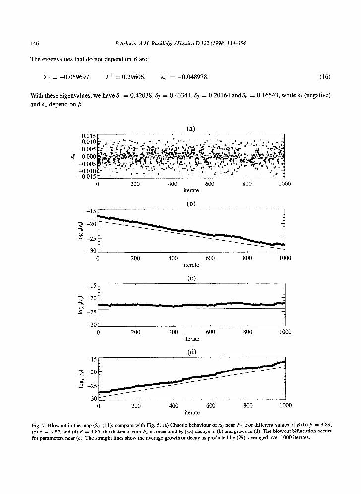
The eigenvalues that do not depend on 13 are:

k t = - 0 . 0 5 9 6 9 7 , L + = 0 . 2 9 6 0 6 , 3+ 2 = - 0 . 0 4 8 9 7 8 . (16)

W i t h t h e s e e i g e n v a l u e s , w e h a v e +l = 0 . 4 2 0 3 8 , 63 = 0 . 4 3 3 4 4 , ~5 = 0 . 2 0 1 6 4 a n d ~6 = 0 . 1 6 5 4 3 , w h i l e ~2 ( n e g a t i v e )

a n d t~ 4 d e p e n d o n 13.

(a) 0.015 ~ + + ++ • J 0 . 0 1 0 ~ - + . + : : ~* ++++ + + +~ + J + + ÷ +++ ÷,~' + % ++++. .÷:+ . ++ . -~ . . . . ~..¢+ +.,. ++ +,',+++_ .,¢ +~.,..,,++ + ++ +.+e÷ ++,.++++?../. ++++~+++.£.~ +~.+.+ .+ +++++.,,.,,..+.,+++_+~ o . t . t u 3 ~ .+ ~ ,+¢+J~+4 + ++ ~;t,,+k~+ t~÷c+ic~ tat~i~t t ~ +Jt+ +'~+;C+'+r-¢ + ¢+t ++"¢÷" +~

• ~+~mP+ ~ . ' , ~ ~ ~a,".r-t ~ .+-~+.,++:nr+Z ~ ' " ~ ~ + ,,+,,'" ++"+-.,'+,,+++ ++,..,,"+...~+ ~ , , ' . , , +-, ~~ Fu~ I~.'+-++~ + ~ ~ ..~'++"+-+"+- .+.t. "+t&+.+t-++'e~+t++ "+,+~+ +",,.,+ +++~..<+++~t ++~'t"'~.~++.'+ +_,.,.+ r,+~ . . . . . +.,,-+++'++.+-+,,.++;+++ +++++++++.+,.+" + ++++ .,,. +u +..,.+*+,,.,. + +.+ + + _++ .,,++ .+y .,,,,- ,+ .,.+.,,+~ - 0 . 0 1 0 ~ +÷ + + ++ ++ +++++ + + + . . . . + + + + _++-,-+ :,.+2 "+ ++- ++~

+- + + + + .I- + ÷ + + , i ,

-0.015 + . . . . . . . . . . . . . . . . . 0 200 400 600 800 1000

iterate

-15 i

~ - 2 0

- 2 5

(b)

- 3 0 L - ~

0 200 400 600 800 1000 iterate

(c)

'5 L j - 2 0

+ _ .

- - - 2 5

- 3 0 . . . . . . . .

0 200 400 600 800 1000 iterate

- 1 5

(d)

~+ - 2 0

t a t )

_o - 2 5

- 3 0 ~ - - 0 200 400 600 800 1000

iterate

Fig. 7. Blowout in the map (8)-(11): compare with Fig. 5. (a) Chaotic behaviour of x0 near Px. For different values of fl (b) fl = 3.89, (c)/~ = 3.87, and (d) fl = 3.85, the distance from Px as measured by lY0[ decays in (b) and grows in (d). The blowout bifurcation occurs for parameters near (c). The straight lines show the average growth or decay as predicted by (29), averaged over 1000 iterates.


0

~ -200

-400

(a)

II[[[[[[[[[[[I ° . . . . . . . . . 100

(b)

-600 0 10000 0 20 40 60 80 100

iterme switch

(c) 0 ~ 1000

-200 - -400

600 -800 .E

-1000 -1200

0

(d)

100 0 20 5• 104 40 60 80 100

iterate switch

Fig. 8. Resonance in the map (8)-(11): compare with Figs. 3 and 6. (a) and (b): fl = 1.100, showing the approach to cycling chaos and the increase in number of iterates between switches (p = 1.011). (c) and (d):/~ = 1.088, showing growth away from cycling chaos (p = 0.9984) and saturation to a periodic orbit. The dashed lines in (c) and (d) show the predicted rate of increase or decrease of the switching times from (39).

4.2. Iterating the map

We seek to reproduce in the map what we have observed in the ODEs: the blowout bifurcation that creates cycling chaos, and the loss of attractiveness of cycling chaos. The first of these (Fig. 7) is straightforward: typical Lorenz-like

chaos is shown in Fig. 7(a), while the change from decay towards Px to growth away from Px at fl ~ 3.87 is shown

in (b)-(d). Cycling chaos is found after the blowout bifurcation (Fig. 8(a)): the system switches between chaos in Px and

chaos in Py, getting closer and closer to the invariant subspaces after each switch and spending longer between

switches (Fig. 8(b)). The rate of increase of the intervals between switches depends on 13, and is about a factor of 1.01 per switch for 13 = 1.10. Decreasing/~ to 1.088 (Figs. 8(c) and (d)) results in growth away from cycling chaos

and saturation to a periodic orbit. These calculations required formulating the map (8)-(11) in terms of the logarithms of the variables in order to

cope with the large (10 l°°°) dynamic range. The one place in which accuracy is inevitably lost is in the switch from

Px to Py (and back), using (10): the C6[yel~61yol ~l term is swamped by the order one x. As a result of this, the chaotic trajectories start in exactly the same way each time the system switches from one invariant subspace to the

other. In terms of the ODEs, the trajectory entering a neighbourhood of Px close to x-rolls shadows the unstable

manifold of that equilibrium point (lying inside Px and leading to the chaotic set Ax) until the switch to Pv. This is

in agreement with the ODE behaviour shown in Fig. 2.


5. Analysis of the blowout bifurcation

We briefly review some definitions. If A is a compact flow-invariant subset then we define the unstable set

}VU(A) = {x ~ R 9 : Or(X) __. A} (17)

and the stable set (or basin of attraction)

~'VS(A) = {x E R 9 : O)(X) __. A}, (18)

where or(x) (resp. w(x)) is the limit set of a trajectory of the ODE passing through x in the limit t ---> -cx~ (resp.

oo). We say a compact invariant set A is an attractor in the sense of Milnor if

£(WS(A)) > 0, (19)

where £(.) is Lebesgue measure on R 9. It is said to be a minimal Miinor attractor if there are no proper compact invariant subsets S C A with e(WS(A)\Ws(s)) > 0 [15].

As shown in [ 1], Milnor attractors can occur in a robust manner if the attractor lies within an invariant subspace.

Suppose P is an invariant subspace and A is a compact invariant set in P such that A is a minimal Milnor attractor

for the flow restricted to P and such that A has a natural ergodic invariant measure # for the flow restricted to P.

It is possible to show (under certain additional hypotheses [1]) that A is an attractor in the full system if and only

if A(lz) < 0, where A is the most positive Liapunov exponent for # in a direction transverse to P (see [5] for a

detailed discussion). If we have access to a normal parameter [5] such that we can vary the normal dynamics without

changing the dynamics in P , we can vary A through zero and observe loss of attractiveness of A at what Ott and Sommerer have termed a blowout bifurcation [16].

5.1. Set criticality of a blowout bifurcation

Ott and Sommerer identify two possible scenarios at blowout. At a supercritical blowout the attractor bifurcates

to a family of attractors displaying on-of f intermittency [17], with trajectories that come arbitrarily close to A and

thus linger near A for long times (but with a well-defined mean length of lingering or 'laminar phase'). At subcritical blowout there are no nearby attractors after loss of stability of A. Note that Ref. [3] discusses the question of how to distinguish these cases.

However, what we see in this paper is that there is at least one other possibility at blowout bifurcation that is

also robust to normal perturbations, namely a bifurcation to a cycling state or a robust heteroclinic cycle between

chaotic invariant sets. This can be seen to be set supercritical but not supercritical, in the following sense.

By reparametrising if necessary we can assume that we have a normal parameter

c = A(~z), (20)

so A undergoes a blowout bifurcation at c = 0. By the argument above, A is an attractor only if c < 0.

If there is a family of minimal Milnor attractors Ac, c > 0 such that for all e > 0

U Ac _ A, (21) c~(O,~)

P Ashwin, A.M Rucklidge/Physica D 122 (1998) 134-154 149

then we say that the blowout is set supercritical. Note that as discussed in [16] and implied by the very word

'blowout', we cannot typically expect the limit of the attractors to just be the set A.

If in addition Ac supports a family of natural ergodic invariant measures #c (c > 0) and/Zc ~ / z as c ~ 0 then

we say the blowout is measure supercritical or just supercritical. (Convergence is in the C* topology on probability

measures.) This definition of criticality was used in [3].

If the blowout is not set supercritical then we say the blowout is subcritical. It seems that one will often get bifurcations in symmetric systems that are set supercritical but not supercritical.

For example one can generically get a blowout from a group orbit of attractors (under a finite group) which yields

a single attractor that limits onto the whole group orbit. Moreover, in the cycling chaos studied here, the attractor

after blowout includes not only the chaotic invariant sets, but also fixed points involved in the heteroclinic cycle.

As it is a cycle, it does not possess a natural ergodic invariant measure [21] and averages of observables from the

system in this state will typically not converge but continue to oscillate more and more slowly.

The blowout scenario described above holds only for variation of normal parameters; in general the varia-

tion of a parameter will affect both the normal dynamics and the dynamics within the invariant subspace. If the

dynamics in the invariant subspace is chaotic, we can expect to see a large number of bifurcations happening

within the invariant subspace and these will cause the blowout to be spread over an interval of parameter values;

there is no reason why A(lzx) should vary continuously with a parameter that varies ~x in a very discontinuous

manner.

Nevertheless, for the numerical results presented in Section 3 the dynamics in the invariant subspace vary in quite

regular way. This is because in our system the parameter/3 is a normal parameter for the attractor Ax; for more discussion of normal parameters, see [5,8].

5.2. Evidence of blowout bifurcation in the ODE model

By mechanisms described in [20] the pure x and y chaotic dynamics corresponding to dynamics within Px and Pv respectively, can become chaotic by means of a symmetric global bifurcation that generates Lorenz-like

attractors approaching the equilibrium solution with full symmetry and x-roll or y-roll equilibrium solutions in Rx or Ry.

Now suppose there exist chaotic attractors Ax and Ay contained in Px and Pv (on the average they have more

symmetry). From here on we will mostly discuss Ax but note that as Ay is a conjugate attractor, the same will hold for Ay.

These attractors contain a saddle equilibrium e in F (the trivial solution) and so in particular they cannot be

Liapunov stable attractors. This is because WU(e) n Px must be non-trivial manifold (otherwise e is an attractor;

thus W u n Pv is also non-trivial as Iso(Py) is conjugate to Iso(Px). Therefore

WU(Ax) ~ Ax, (22)

and so Ax cannot be Liapunov stable. However, it is possible that Ax is an attractor in the sense of Milnor; this will imply that the basin will be locally riddled in the sense of [5].

We assume that Ax and Ay are minimal Milnor attractors containing e. We also assume that they have natural

ergodic invariant measures/Zx and #y supported on them. We now concentrate on Ax. Whether Ax is an attractor

depends on its the spectrum of normal Liapunov exponents. Note that the zero Liapunov exponent corresponding to time translation always corresponds to a perturbation tangential to the invariant subspace. If

A(#x) < 0, (23)


where A (#) is the most positive normal Liapunov exponent for the measure IX, it is possible to show that Ax satisfies (19) [5], and hence that Ax is a Milnor attractor.

It is comparatively easy to compute A(IXx) in that case, as the largest transverse Liapunov exponent of Ax in the parameter regime discussed corresponds to directions in the Qx direction, where linearised perturbations are described by

Yo = (Ix + O(t) - /sxo(t)2)yo. (24)

Thus we can see that

A(Ixx) = Ix + (O).x - / 5 ( x Z ) . x , (25)

where ( f ( x ) ) u = f f ( x ) dIx(x). From the equation for 0 it is possible to show that

T T

if lim 0 dt = lim -- Xo 2 dt (26) T--+~ T T--+~ T

along bounded trajectories of the ODE. For the given parameter values it is possible to approximate (O)ux = -0 .03703 and so (x2)ux = 0.03703. Thus

A(Ixx) = Ix - (x2)ux - /5(x2)ux = 0.12847 - 0.03703/5, (27)

implying that the blowout bifurcation occurs at approximately/5 = 3.47, which is in good agreement with the

simulations (Fig. 5(b)). Note that whenever e is hyperbolic and within the attractor Ax there exists at least one ergodic invariant measure

Ixe (in particular that one supported on e) such that A(Ixe) > 0. In particular, this means that the basins of the

attractors Ax and Ay are riddled for all parameter values in our problem!

Likewise, in the map (8) near Px, the logarithm of Y0 obeys

log lYol ~ log lY01 + log C2 + 82 log [x0l, (28)

where 82 is a function of/5. The most positive normal Liapunov exponent in this case is then

A = log C2 + 82(log Ix01), (29)

where the average is taken over the Lorenz attractor. Averaging over 107 iterates of (7) yields (log Ix01) = -5 .9233 and, solving (29) for/5, we obtain/5 = 3.869 at the blowout bifurcation, in agreement with the data in

Fig. 7(b). As A(Ixx) passes through 0, Ax loses stability and becomes a chaotic saddle, and in doing so it creates a

continuum of connections from Ax to the fixed point (y-rolls) in Ry. These connections are robust to G-equivariant perturbations, as y-rolls are sinks within Qx, and so there is a robust cycle alternating between the equilibrium

points in Rx and Ry and the chaotic sets in Px and Py. We observed in Sections 3 and 4 that this cycling chaos is attractive once it is created; we turn to the stability of

cycling chaos in the next section.

6. Analysis of the resonance of cycling chaos

It is clear from Figs. 3, 6 and 8 that the key to understanding the loss of stability of cycling chaos lies in obtaining the rate at which trajectories approach that state. It is possible to estimate this rate for the map, and we


use information gained in this calculation to carry out the same estimate in the ODEs, and thus are able to obtain the values of/3 at which the loss of stability occurs, in the map and in the ODEs. What is remarkable is that, once a single average over Ax has been computed numerically, the value of/~ at the bifurcation point can be obtained analytically.

6.1. Rate of approach to cycling chaos

We suppose that (in the map) the system arrives near Px with given values of (xo, 1, Yo, Y2), iterates using (8) n times (n >> 1), ending up in a state (x~, 1, y~, y~) with lY~I > [x~l. There follows one iterate of (10), leaving the system near Py inastate (x 0," x2," Yo," 1) (we are ignoring changesofsignofthevariables).Weneedto establish an estimate of (x~', x~'), a measure of the distance from Py, given that (yo, y2) were small when the system started close to Px.

Properly, the value of y~ after n iterates will depend on the values of xo over those n iterates, but if n is large, we approximate the detailed history of xo by its average and obtain

log lY~I = log lYol + nAe,

log lY~I = log lY21 + nAc,

(30)

(31)

where

Ae = log C2 + Be(log Ix01), (32)

Ac = log C3 + 33 (log Ix01) (33)

are Liapunov exponents in the expanding and contracting directions around Px. Ae is precisely the Liapunov exponent that went through zero at the blowout bifurcation in (29). Note that we have effectively approximated the chaotic set Ax by an equilibrium point.

The trajectory escapes from the neighbourhood of Px once l Y~I > I x~l; since x0 is typically of order one (compared to the tiny initial value of Y0), we assume that the escape takes place when lY~I = 1, so obtaining

1 n = - A---T log ly01, (34)

Ac log lYe[ = log lY21 -Aee log lY01, (35)

t and ~ both of order one. with x 0 Y0 One iterate of (10) now yields

log Ix~'l = log Ix~l + logf4 + 32 log lY~I + 341og lY~I, (36)

log Ix~'l = log C5 + 33 log lY~I + 35 log lY~I. (37)

These expressions will be dominated by log lY~[ once the trajectory is very close to the heteroclinic cycle, so, neglecting terms of order one, we obtain

log Ix~'l [ - 3 4 - ~ 34 ] ( log ly0l ) _t_ O(1) ' (38) ) loglx~11, -35A~ 35 ~l°glY2l

for large negative values of log lyol and log ly21. A conjugate map will describe the return from Py to p~. One eigenvalue of the matrix is zero because of the way we approximated the behaviour near the chaotic set; the other eigenvalue is


8 Ac (39) p = 85 - - 4 A e '

which we refer to as the stability index. The zero eigenvalue forces log Ix~'[ = (84/85) log [x~2'l, so after one iterate of the composite map (38), the dynamics

will obey

log Ix;'[ ) ( l o g ly0[) (40) Ioglx~'l = p \ log ly21 '

Clearly if p > 1, log Ix01 and log ly01 will tend to - o o and the trajectory will asymptote to attracting cycling chaos. Conversely, if p < 1, cycling chaos is unstable and trajectories will leave the domain of validity of the approximations we have made. We can also deduce from (34) that the number of iterates between each switch will increase by a factor of p per switch.

At the point at which cycling chaos is created (as Ae increases through zero), we see that p is much greater than one, provided that Ac is negative and 84 is positive, both of which are true in the examples we have discussed. We deduce that cycling chaos is attracting near to its creation at the blowout bifurcation.

6.2. Loss of stability of cycling chaos

From the condition that p = 1 at the loss of stability of the chaotic cycle, we determine that this bifurcation occurs in the map at/3 = 1.0896, in agreement with the data in Fig. 8.

Returning to the ODEs, we observe that in (39) 84 and 85 are ratios of eigenvalues of x-rolls (proportional to

decay rates of Y0 and Yx), while Ae and Ac are the growth rate of Y0 and the decay rate of Y2 near the chaotic set Ax. In the ODEs, the linearisation of (1) about Ax yields ~ for the decay rate of Y2, while the growth rate of Y0 is given by (29). Hence we have the stability index

85 - - 84 A-~-~e~ e (41) P

for the ODEs, where Ae is given by (29). Note that 84 and Ae are both functions of/3. The condition p = 1 is readily solved for/3, and has solution/3 = 1.63. At/3 = 1.63 the ODEs are still approaching cycling chaos, with switching times increasing by a factor of above 1.02 per switch (see Fig. 6). However, the ODEs have not yet reached their asymptotic rate of slowing down, resolving this small discrepancy.

On decreasing/3 below 1.63, the stability index p decreases below unity and the cycling chaos will no longer be attracting. This loss of stability can broadly be classed as a resonance of Liapunov exponents. Observe that the resonance will be located at different/3 for different invariant measures supported on Ax,y and so we expect the presence of riddling and associated phenomena found in [2] at a resonance of a simpler model displaying cycling chaos.

We note that constructing and analysing the map was required in order to determine the combination of eigenvalues and Liapunov exponents that governs the stability index p in the ODEs.

We observe that for/3 below the resonance bifurcation, the system exhibits behaviour that is numerically indistin- guishable from periodic: there appear to be a large number of coexisting apparently periodic orbits. We hypothesize that the resonance creates a branch of 'approximately periodic attractors', i.e., attractors that have a well-defined finite mean period of passage around the cycle, going to infinity at the resonance [2]. These might lock onto long periodic orbits for progressively smaller/3, as found in the numerical simulations. For this example, the approximately periodic attractor branches set supercritically from the cycling chaos; however, one presumes that subcritical


branching is also possible. Research is presently in progress on understanding the more detailed branching behaviour at this bifurcation.

7. Discussion

This study has shown that one possible, apparently generic scenario for loss of stability of a chaotic attractor in

an invariant subspace on varying a normal parameter is as follows: there is a blowout bifurcation that creates an attracting, robust heteroclinic cycle between chaotic invariant sets (cycling chaos). The bifurcation is set supercritical

but not supercritical, i.e., the bifurcated attractors contain the attractor for the system in the invariant subspace,

but unlike in a supercrifical bifurcation (to an on-off intermittent state) the length of laminar phases increases unboundedly along a single trajectory even at a finite distance from the blowout.

This cycling chaotic state can be modelled well by the network shown in Fig. 4 although in reality the network is complicated by the facts that (a) there are other fixed points contained in the closure of unstable manifolds and

(b) the fixed points in Rx and Ry are actually contained in the chaotic sets Ax and Ay rather than being isolated. We suspect this may have the consequence that there is no Poincar6 section to the flow and so the cycle is 'dirty' in the terminology of [2]. Nevertheless, the normal Liapunov spectrum of the invariant chaotic set seems to determine the attraction or not of the cycle.

The attracting cycling chaos is observed to lose stability via a mechanism that resembles a resonance of eigenvalues

in an orbit heteroclinic to equilibria. Such a resonance has been seen to occur in special classes of systems with skew product structure [2], in analogy to the branching of periodic orbits at a homoclinic resonance investigated by [7].

Throughout this investigation, it has been necessary to monitor carefully several numerical effects. In particular, for trajectories that display asymptotic slowing down characteristic of cycling chaos there will be a point at which rounding errors cause the dynamics either to transfer to the invariant subspace, or keep the dynamics a finite distance

from the invariant subspace. In the context of physical systems there will always be imperfections in the system and noise that will destroy the invariant subspaces. Nevertheless the perfect symmetry model will be very useful in describing what one expects to see in such imperfect situations.

It still remains to prove rigorously that the observed scenario is generic and so of interest to other, less specific models and in particular PDE models of which this is a truncation. We would like to emphasise that the behaviour

we see occurs for a reasonably large region of physically relevant parameters in the ODE model and moreover we are unaware of any other classification which explains and predicts the observed dynamics to the degree that we

have done here. In principle, cycling chaos can be seen in ODE models down to dimension 4, though not smaller than this; thus this dynamics should be seen as something that will not be created at a generic bifurcation from a trivial state, but rather in a more complicated dynamical regime far from primary bifurcation.

We have discussed a possible route to cycling chaos through a blowout bifurcation, and how cycling chaos might cease to be attracting, both in general terms and in the context of a specific model. Our general results ought to be applicable to a variety of other problems. In particular, behaviour that might be understood in terms of cycling

chaos has been seen by Knobloch et al. [12] in an ODE model of the dipole~quadrupole interaction in the solar dynamo. In their model, there is a weakly broken symmetry between the dipole and quadrupole subspaces, and the system switches between the two subspaces, favouring one over the other since they are not equivalent.

Finally, one comment that deserves to be made is that the choice of/3 as the parameter allows an important simplification because of this parameter is normal for dynamics within Px and Py. One assumes that similar

behaviour will be observed for non-normal parameters with the exception that the chaos in the invariant subspace will be fragile [6] and destroyed by many arbitrarily small perturbations; see [8].

154

Acknowledgements

P. Ashwin, A.M. Rucklidge / Physica D 122 (1998) 134-154

We acknowledge very interest ing conversat ions with Mike Field, Marty Golubi tsky and Edgar Knobloch con-

cerning this work. The research of PA was partially supported by a Nuffield 'Newly Appoin ted Science Lecturer '

award and EPSRC grant GR/K77365. A M R is grateful for support f rom the Royal Ast ronomica l Society.

References

[1] J.C. Alexander, I. Kan, J.A. Yorke, Zhiping You, Riddled basins, Int. J. Bifur. and Chaos 2 (1992) 795-813. [2] P. Ashwin, Cycles homoclinic to chaotic sets; robustness and resonance, Chaos 7 (1997) 207-220. [3] P. Ashwin, P. Aston, M. Nicol, On the unfolding of a blowout bifurcation, Physica D 111 (1998) 81-95. [4] P. Ashwin, J. Buescu, I.N. Stewart, Bubbling of attractors and synchronisation of oscillators, Phys. Lett. A 193 (1994) 126-139. [5] P. Ashwin, J. Buescu, I.N. Stewart, From attractor to chaotic saddle: a tale of transverse instability, Nonlinearity 9 (1996) 703-737. [6] E. Barreto, B. Hunt, C. Grebogi, J. Yorke, From high dimensional chaos to stable periodic orbits: the structure of parameter space,

Phys. Rev. Lett. 78 (1997) 4561--4564. [7] S.-N. Chow, B. Deng, B. Fiedler, Homoclinic bifurcation at resonant eigenvalues, J. Dyn. Diff. Eqns. 2 (1990) 177-244. [8] E. Covas, P. Ashwin, R. Tavakol, Non-normal parameter blowout bifurcation: an example in a truncated mean-field dynamo model,

Phys. Rev. E 56 (1997) 6451--6458. [9] M. Dellnitz, M. Field, M. Golubitsky, A. Hohmann, J. Ma, Cycling chaos, IEEE Trans. Circuits and Systems-142 (1995) 821-823.

[10] M. Field, Lectures on Bifurcations, Dynamics and Symmetry, Pitman Research Notes in Mathematics, vol. 356, Pitman, London, 1996.

[11] J. Guckenheimer, P. Holmes, Structurally stable heteroclinic cycles, Math. Proc. Camb. Phil. Soc. 103 (1988) 189-192. [ 12] E. Knobloch, S.M. Tobias, N.O. Weiss, Modulation and symmetry changes in stellar dynamos, Mort. Not. Roy. Astr. Soc. 297 (1998)

1123-1138. [13] M. Krupa, I. Melbourne, Asymptotic stability of heteroclinic cycles in systems with symmetry, Ergod. Th. Dyn. Sys. 15 (1995)

121-147. [14] P.C. Matthews, A.M. Rucklidge, N.O. Weiss, M.R.E. Proctor, The three-dimensional development of the shearing instability of

convection, Phys. Fluids 8 (1996) 1350-1352. [15] J. Milnor, On the concept of attractor, Commun. Math. Phys. 99 (1985) 177-195; Comments, Commun. Math. Phys. 102 (1985)

517-519. [16] E. Ott, J.C. Sommerer, Blowout bifurcations: the occurrence of riddled basins and on-off intermittency, Phys. Lett. A 188 (1994)

39-47. [17] N. Platt, E.A. Spiegel, C. Tresser, On-off intermittency: a mechanism for bursting, Phys. Rev. Lett. 70 (1993) 279-282. [18] W.H. Press, B.P. Flannery, S.A. Teukolsky, W.T. Vetterling, Numerical Recipes - The Art of Scientific Computing, Cambridge

University Press, Cambridge, 1986. [19] A.M. Rucklidge, P.C. Matthews, The shearing instability in magnetoconvection, in: A. Brandt, H.J.S. Fernando (Eds.) Double-

Diffusive Convection, American Geophysical Union, Washington, 1995, pp. 171-184. [20] A.M. Rucklidge, P.C. Matthews, Analysis of the sheafing instability in nonlinear convection and magnetoconvection, Nonlinearity

9 (1996) 311-351. [21] K. Sigmund, Time averages for unpredictable orbits of deterministic systems, Ann. Opera. Res. 37 (1992) 217-228.

Documents

Cycling chaos: its creation, persistence and loss of stability in a model of nonlinear magnetoconvection