Cybersecurity Insurance: Modeling and Pricing...has been reiterated in the workshop and roundtable of the US Department of Homeland Security’s (DHS) National Protection and Programs

Cybersecurity Insurance: Modeling and Pricing

March 2017

2

Copyright © 2017 Society of Actuaries


Maochao Xu Department of Mathematics Illinois State University, USA Lei Hua, ASA Division of Statistics Northern Illinois University, USA

Caveat and Disclaimer The opinions expressed and conclusions reached by the authors are their own and do not represent any official position or opinion of the Society of Actuaries or its members. The Society of Actuaries makes no representation or warranty to the accuracy of the information. Copyright © 2017 by the Society of Actuaries. All rights reserved.

3


Contents

Acknowledgments ................................................................................................................. 4

Section 1: Introduction and Motivation ................................................................................. 4

Section 2: Models for Cybersecurity Risks .............................................................................. 7

Section 3: Epidemic Spreading Models ................................................................................... 8 3.1 Markov Model ..........................................................................................................................9 3.2 Non-Markov Model ................................................................................................................ 12

Section 4: Simulation and Pricing ......................................................................................... 19 4.1 Independent Cybersecurity Risks ............................................................................................. 21

4.1.1 Exponential Distribution ............................................................................................................ 21 4.1.2 Weibull Distribution ................................................................................................................... 23 4.1.3 Log-normal Distribution ............................................................................................................. 26

4.2 Dependent Cybersecurity Risks ............................................................................................... 28 4.2.1 Gaussian Copula ......................................................................................................................... 28 4.2.2 Clayton Copula ........................................................................................................................... 30

4.3 Pricing .................................................................................................................................... 32

Section 5: Conclusion ........................................................................................................... 35

References .......................................................................................................................... 36

4



Cybersecurity risk has attracted considerable attention in recent decades. However, modeling the cybersecurity risk

is still in its infancy, mainly because of its unique characteristics. In this paper, we develop a framework for modeling

and pricing cybersecurity risk. The proposed model consists of three components: epidemic models, loss functions

and premium strategies. We study the dynamic upper bounds for the infection probabilities based on both Markov

and non-Markov models. A simulation approach is proposed to compute the premium for the cybersecurity risk for

practical use. The effects of different infection distributions and dependence among infection processes on the

losses are studied as well.

Acknowledgments The authors are very grateful to the members of the Project Oversight Group for their insightful and constructive

comments, which led to this improved version of the paper. This research is supported by the Society of Actuaries

(SOA). Any opinions, findings, and conclusions or recommendations expressed in this material are those of the

authors and do not necessarily reflect the views of SOA.

Section 1: Introduction and Motivation Cybersecurity insurance, which is designed to transfer the economic losses associated with network and computer

incidents to a third party, has attracted much attention from professionals and researchers recently. The problem

has been reiterated in the workshop and roundtable of the US Department of Homeland Security’s (DHS) National

Protection and Programs Directorate (NPPD) (2012, 2013) [8]. The eighth Emerging Risks Survey by the Society of

Actuaries indicates that, according to risk managers, cybersecurity risk is the greatest emerging risk. The

cybersecurity insurance market continues to broaden, and more and more small to midsize companies show interest

in cybersecurity insurance. Many companies are seeking coverages for the value of data loss, lost revenue due to

loss of data or downtime, legal expenses for damage to the third party, notification of potentially affected customers

and regulatory fines and penalties [13, 2]. It is estimated that the annual gross written premium is $3.25 billion for

2016, compared to $2.75 billion in 2015 [2]. However, the contributions to modeling the cybersecurity risk in the

literature are largely descriptive, which is mainly because cyber risk is very different from the traditional risks

covered by indemnity insurance. The significant property that distinguishes cyber risk from conventional risk is that

information and communication technology (ICT) resources are interconnected in a network, and therefore the

analysis of risk and its related potential losses needs to take into account the network topology. Further, if ICT

resources are hijacked, then benign sources (e.g., computers) may become threats to other sources [4].

Traditionally, pricing insurance products relies on actuarial tables constructed from historical records. Unlike

traditional insurance policies, however, cybersecurity insurance has no standard scoring systems or actuarial tables

5


for rate making. Cybersecurity risks are relatively new, and the data about security breaches and losses do not exist

or exist only in small quantities. This difficulty may be further exacerbated by the reluctance of organizations to

reveal details of security breaches due to loss of market share, loss of reputation and so forth. Pricing cybersecurity

risks is still a challenging question, although many insurance companies do provide cybersecurity insurance products.

The insurers tend to increase the premiums for the larger companies, and the coverage may be limited and very

expensive for the companies without good cybersecurity protection [2].

The literature reveals several efforts to study the cybersecurity risk via mathematical models. For example, Gordon

et al. [11] discuss a general framework on pricing and the adverse selection issues of cyber insurance, and they

propose a four-step cyber risk decision plan. Bohme and Kataria [3] consider the correlation between cyber risks and

use the beta-binomial and one-factor latent risk model for modeling purposes. In particular, Bohme and Kataria

discuss the internal correlation of cybersecurity risk within a firm and the global correlation of cybersecurity risk at

the global level. Bohme and Schwartz [4] discuss a framework for dealing with the specific properties of cybersecurity

risk, including interdependent security, correlated risk and information asymmetry. They also present a survey on

existing models of cybersecurity insurance. A discrepancy between informal arguments in favor of cybersecurity

insurance as a tool to improve network security is discussed there.

A Bayesian brief network approach is proposed in Mukhopadhyay et al. [17] for modeling the cybersecurity risk.

They use the multivariate Gaussian copula to model the joint distribution and conditional distribution of each node

on the network. The premiums are calculated as a function of expected value of claim severity. Herath and Herath

[12] propose a copula-based actuarial model for pricing cybersecurity risk, where they model three risk variables:

occurrence of the event, the time of payment and the amount of payment. The premiums for first-party losses due

to epidemic attacks are calculated by using three types of insurance policy models: policy with a zero deductible,

policy with deductibles and policy with coinsurance and limits. Schwartz and Sastry [22] present a framework for

managing cybersecurity risk in a large-scale interdependent network. They consider the cyber insurers as strategic

players, and they derive the solution for user optimal security in environments with and without cyber insurers.

Yang and Lui [29] use the Bayesian network game to model the security investment, where the network externality

effect is considered. It is shown there that nodes with more degrees are more likely to be infected and have higher

chances to be affected by others’ decisions. One may refer to Kosub [16] and Eling and Schnell [10] for

comprehensive reviews on cybersecurity risk modeling and management of cybersecurity risk.

Our work in this paper is different from those in the literature in the following aspects: (1) We use stochastic

processes (Markov and non-Markov) to describe the dynamics of epidemic spreading over time, while most of the

aforementioned works are static. (2) We propose to use the copula to capture the dependence among the time-to-

6


infection distributions, whereas in the literature it is often assumed to be independent. (3) We suggest using Monte

Carlo simulations to evaluate the security level of networks, and the security level includes the number of incidents,

the infection probabilities of nodes and the total losses.

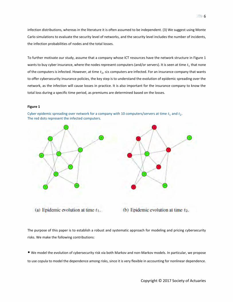
To further motivate our study, assume that a company whose ICT resources have the network structure in Figure 1

wants to buy cyber insurance, where the nodes represent computers (and/or servers). It is seen at time 𝑡1 that none

of the computers is infected. However, at time 𝑡2, six computers are infected. For an insurance company that wants

to offer cybersecurity insurance policies, the key step is to understand the evolution of epidemic spreading over the

network, as the infection will cause losses in practice. It is also important for the insurance company to know the

total loss during a specific time period, as premiums are determined based on the losses.

Figure 1

Cyber epidemic spreading over network for a company with 10 computers/servers at time 𝑡1 and 𝑡2. The red dots represent the infected computers.

The purpose of this paper is to establish a robust and systematic approach for modeling and pricing cybersecurity

risks. We make the following contributions:

• We model the evolution of cybersecurity risk via both Markov and non-Markov models. In particular, we propose

to use copula to model the dependence among risks, since it is very flexible in accounting for nonlinear dependence.

7


• We study the dynamic upper bounds for the infection probabilities of nodes over time. We show that the

independence assumption among risks would lead to upper bounds for the infection probabilities.

• We propose to use Monte Carlo simulations to study the pricing strategies in practice. Specifically, we simulate

the evolution of epidemic spreading over a network, and hence, derive three key quantities: the number of incidents,

the infection probabilities and the total losses.

The rest of the paper is organized as follows. Section 2 discusses the framework for modeling cybersecurity risks by

using a renewal process. In Section 3, the evolution of epidemic spreading is modeled by both Markov and non-

Markov models, and some upper bounds are discussed. Section 4 presents the simulation and pricing strategies. In

the last section, we conclude our results and present some points for discussion.

Section 2: Models for Cybersecurity Risks Assume that a company has a network that could be described as an undirected graph Γ = (𝑉; 𝔼), where 𝑉 is the

node set and 𝔼 is the edge set. Note that Γ abstracts the network structure according to which the cyber attacks

take place (e.g., malware spreading), where (𝑢, 𝑣) ∈ 𝔼 abstracts that nodes 𝑢 and 𝑣 can attack each other

(undirected graph). In principle, Γ can range from a complete graph (i.e., any 𝑢 ∈ 𝑉 can attack any 𝑣 ∈ 𝑉) to any

specific graph structure. Denote by 𝐴 = (𝑎𝑣𝑢) the adjacency matrix of Γ, where 𝑎𝑣𝑢 = 1 if and only if (𝑢, 𝑣) ∈ 𝔼,

and 𝑎𝑣𝑢 = 0 otherwise. Note that the problem setting naturally implies 𝑎𝑣𝑣 = 0. Denote by 𝑑𝑒𝑔(𝑣) the degree of

node 𝑣, and 𝑁 = |𝑉| the total number of nodes. Node 𝑣 ∈ 𝑉 is either secure (but vulnerable to attacks) or infected

(and can attack other nodes) at any time 𝑡 = 0,1, ⋯. The status of this network at time t can be represented as

(𝐼1(𝑡), ⋯ , 𝐼𝑁(𝑡))

where 𝐼𝑣(𝑡) = 1 represents that node v is in infection status at time t, while 𝐼𝑣(𝑡) = 0 represents that node 𝑣 is

secure at time 𝑡. The infection probability vector is denoted by

𝒑𝑇(𝑡) = (𝑝1(𝑡), ⋯ , 𝑝𝑁(𝑡)),

where 𝑝𝑗(𝑡) = 𝑃(𝐼𝑗 = 1), for 𝑗 = 0,1, ⋯ , 𝑁.

We consider two threats faced by each node: (1) threats outside the network (i.e., node 𝑣 is infected because it is

attacked or its user visits a malicious website); and (2) threats inside the network (i.e., node 𝑣 is infected, then node

𝑣 attacks its neighbors). We also assume that if node 𝑣 is infected, it will be repaired or cleaned to return to secure

status. Extensive work has been done modeling the epidemic spreading over the network in the communities of

physics and cybersecurity. One may refer to [1, 26, 28, 27, 19] for comprehensive discussions and reviews on this

topic.

8


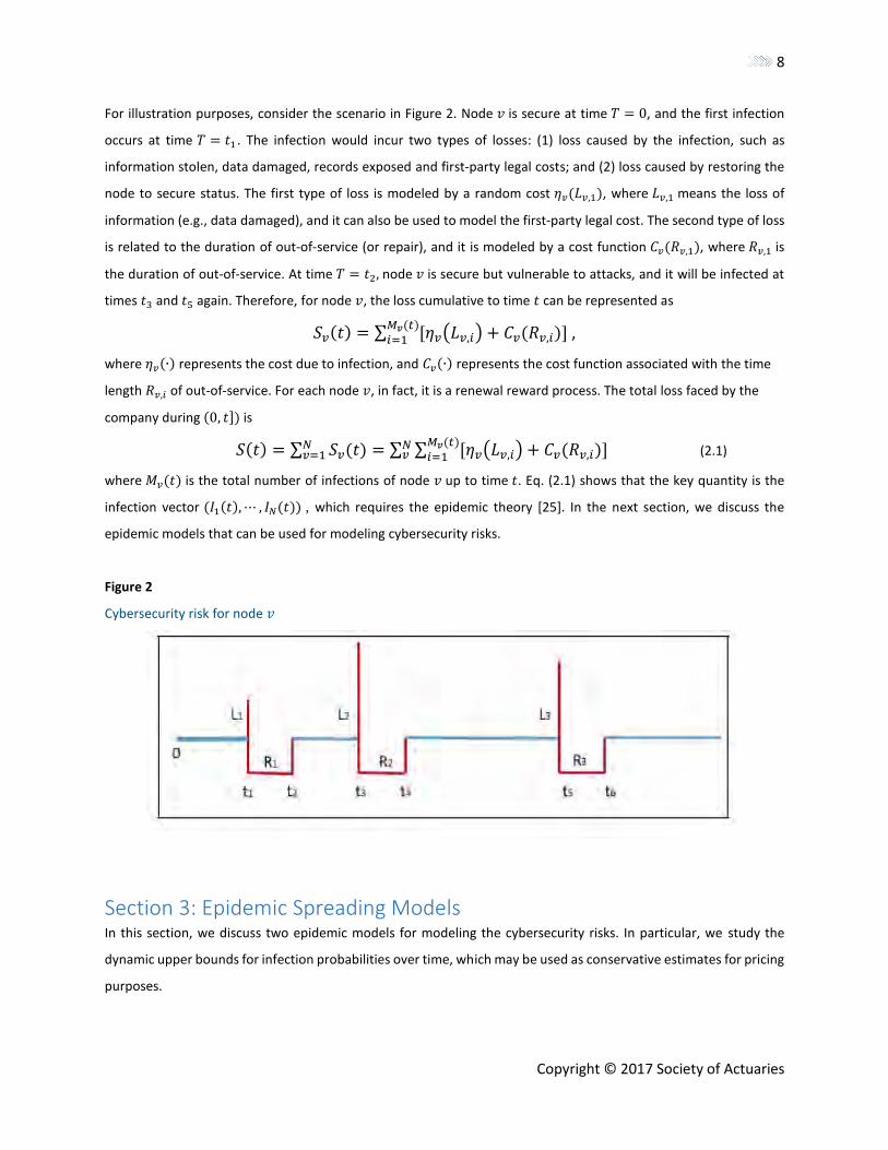
For illustration purposes, consider the scenario in Figure 2. Node 𝑣 is secure at time 𝑇 = 0, and the first infection

occurs at time 𝑇 = 𝑡1 . The infection would incur two types of losses: (1) loss caused by the infection, such as

information stolen, data damaged, records exposed and first-party legal costs; and (2) loss caused by restoring the

node to secure status. The first type of loss is modeled by a random cost 𝜂𝑣(𝐿𝑣,1), where 𝐿𝑣,1 means the loss of

information (e.g., data damaged), and it can also be used to model the first-party legal cost. The second type of loss

is related to the duration of out-of-service (or repair), and it is modeled by a cost function 𝐶𝑣(𝑅𝑣,1), where 𝑅𝑣,1 is

the duration of out-of-service. At time 𝑇 = 𝑡2, node 𝑣 is secure but vulnerable to attacks, and it will be infected at

times 𝑡3 and 𝑡5 again. Therefore, for node 𝑣, the loss cumulative to time 𝑡 can be represented as

𝑆𝑣(𝑡) = ∑ [𝜂𝑣(𝐿𝑣,𝑖) + 𝐶𝑣(𝑅𝑣,𝑖)]𝑀𝑣(𝑡)𝑖=1 ,

where 𝜂𝑣(∙) represents the cost due to infection, and 𝐶𝑣(∙) represents the cost function associated with the time

length 𝑅𝑣,𝑖 of out-of-service. For each node 𝑣, in fact, it is a renewal reward process. The total loss faced by the

company during (0, 𝑡]) is

𝑆(𝑡) = ∑ 𝑆𝑣(𝑡)𝑁𝑣=1 = ∑ ∑ [𝜂𝑣(𝐿𝑣,𝑖) + 𝐶𝑣(𝑅𝑣,𝑖)]

𝑀𝑣(𝑡)𝑖=1

𝑁𝑣 (2.1)

where 𝑀𝑣(𝑡) is the total number of infections of node 𝑣 up to time 𝑡. Eq. (2.1) shows that the key quantity is the

infection vector (𝐼1(𝑡), ⋯ , 𝐼𝑁(𝑡)) , which requires the epidemic theory [25]. In the next section, we discuss the

epidemic models that can be used for modeling cybersecurity risks.

Figure 2

Cybersecurity risk for node 𝑣

Section 3: Epidemic Spreading Models In this section, we discuss two epidemic models for modeling the cybersecurity risks. In particular, we study the

dynamic upper bounds for infection probabilities over time, which may be used as conservative estimates for pricing

purposes.

9


3.1 Markov Model For this model, we assume the recovering process of any infected node 𝑣 is a Poisson process with 𝛿𝑣. The infection

process per link is also a Poisson process with 𝛽 due to the infected neighbors inside the network. We also assume

that for any infected node, it may be infected with a Poisson 𝜖𝑣 due to the threat outside the network. The infection

processes and recovering processes are assumed to be independent. This model, in fact, is known as 𝜖-SIS model

[26] or push-pull model [27] in the literature. For any node 𝑣, the infection and recovery processes form the following

Markov process:

𝐼𝑣(𝑡) = 0 → 1 at rate 𝛽 ∑ 𝑎𝑣𝑗𝐼𝑗(𝑡) + 𝜖𝑣𝑛𝑗=1 ;

𝐼𝑣(𝑡) = 1 → 0 at rate 𝛿𝑣.

The following result provides a dynamic upper bound for infection probabilities, which may be used as a conservative

estimate for infections over the network.

Theorem 3.1 Let 𝑄 = diag((𝛽𝛿𝑣)/(𝛿𝑣 + 𝜖𝑣))𝐴 − diag(𝛿𝑣 + 𝜖𝑣). Then the dynamic upper bound for

the infection probability is

𝑝∗(𝑡) = 𝑒𝑄𝑡𝑝∗(0) + 𝑄−1(𝑒𝑄𝑡 − 𝐼)𝝐,

where 𝜖𝑇 = (𝜖1, ⋯ , 𝜖𝑛), and

𝑒𝑄𝑡 = ∑𝑄𝑡𝑘𝑡

𝑘!

∞𝑘=1 .

Proof: The epidemic spreading process can be written as the following master equation:

𝑑𝔼[𝐼𝑣(𝑡)]

𝑑𝑡= 𝔼[(1 − 𝐼𝑣(𝑡))(𝛽 ∑ 𝑎𝑣𝑗𝐼𝑗(𝑡) + 𝜖𝑣

𝑁𝑗=1 )] − 𝛿𝑣𝔼[𝐼𝑣(𝑡)], 𝑣 = 1, ⋯ , 𝑁. (3.1)

That is,

𝑝𝑣′ (𝑡) = 𝔼[(1 − 𝐼𝑣(𝑡))(𝛽 ∑ 𝑎𝑣𝑗𝐼𝑗(𝑡) + 𝜖𝑣

𝑁𝑗=1 )] − 𝛿𝑣𝔼[𝐼𝑣(𝑡)],

which could be rewritten as

𝑝𝑣′ (𝑡) = 𝛽 ∑ 𝑎𝑣𝑗𝑝𝑗(𝑡) + 𝜖𝑣

𝑁𝑗=1 − 𝛽 ∑ 𝑎𝑣𝑗𝔼[𝐼𝑗(𝑡)𝐼𝑣(𝑡)]𝑁

𝑗=1 − 𝜖𝑣𝑝𝑣(𝑡) − 𝛿𝑣𝑝𝑣(𝑡).

Note that the dependence among 𝐼𝑗(𝑡) and 𝐼𝑣(𝑡) are generally positive [6]. Then we have

𝑝𝑣′ (𝑡) ≤ 𝛽 ∑ 𝑎𝑣𝑗𝑝𝑗(𝑡) + 𝜖𝑣

𝑁𝑗=1 − (𝛿𝑣 + 𝜖𝑣)𝑝𝑣(𝑡) − 𝛽 ∑ 𝑎𝑣𝑗𝑝𝑗(𝑡)𝑝𝑣(𝑡)𝑁

𝑗=1 . (3.2)

It can be represented in the matrix form as

𝒑(𝑡) ≤ [𝛽𝐴 − 𝑑𝑖𝑎𝑔(𝛿𝑣 + 𝜖𝑣)]𝒑(𝑡) + 𝝐 − 𝛽𝑑𝑖𝑎𝑔(𝑝𝑣(𝑡))𝐴𝒑(𝑡).

Note that, for any 𝑡 ≥ 0,

𝑝𝑣(𝑡) ≥𝜖𝑣

𝛿𝑣+𝜖𝑣 , 𝑣 = 1, ⋯ , 𝑁.

This is because we could consider the infection 𝛽 = 0, which would lead to a two-state continuous Markov chain.

Now, let

10


𝑄 = diag (𝛽𝛿𝑣

𝛿𝑣+𝜖𝑣) 𝐴 − diag(𝛿𝑣 + 𝜖𝑣).

Therefore, it holds that

𝒑′(𝑡) ≤ 𝑄𝒑(𝑡) + 𝝐.

Consider the following equation:

𝒑∗′(𝑡) − 𝑄𝒑∗(𝑡) = 𝝐. (3.3)

This is a nonhomogeneous linear differential equation of order 1, and it can be solved explicitly as follows:

𝒑∗(𝑡) = 𝑒𝑄𝑡𝒑∗(0) + ∫ 𝑒𝑄(𝑡−𝑠)𝝐𝑑𝑠𝑡

0

= 𝑒𝑄𝑡𝒑∗(0) + 𝑄−1[𝑒𝑄𝑡 − 𝐼]𝝐

where

𝑒𝑄𝑡 = ∑𝑄𝑡𝑘𝑡

𝑘!

∞𝑘=0 .

Note that given the same initial probabilities 𝒑∗(0) = 𝒑(0), it holds that 𝒑(𝑡) ≤ 𝒑∗(𝑡) for any 𝑡 > 0. The proof is

completed. ∎

Remarks: Note that 𝑄 is symmetric, and it can be diagonalized as

𝑄 = 𝑀𝐷𝑀−1,

where 𝑀 is a real orthogonal matrix and 𝐷 is a diagonal matrix. If all eigenvalues of the matrix 𝑄 have a negative

real part, then Eq. (3.3) is stable [7], and the solution of Eq. (3.3) could be rewritten as

𝒑∗(𝑡) = 𝒑∗ + 𝑒𝑄𝑡[𝒑∗(0) − 𝒑∗],

where 𝒑∗ = −𝑄−1𝝐 if 𝑄 is invertible.

To illustrate, we present the following examples. For different scenarios presented in the paper, we use letter 𝑀for

those based on Markov models and 𝑁 for those based on non-Markov models.

Example 3.2 Consider the network in Figure 1. For simplicity, we assume that all the nodes have the same infection

and recovery rates.

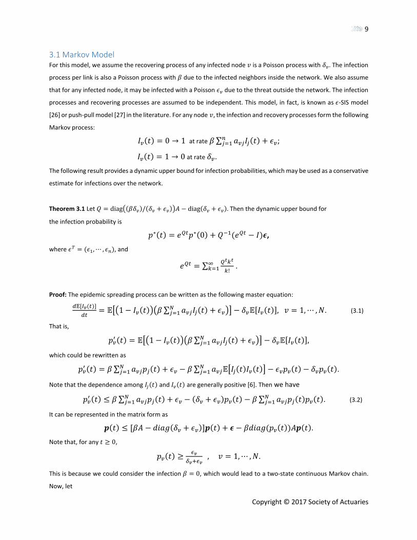
• Scenario M1: Assume the initial infection probability is 0, and 𝛽 = .01, 𝜖 = .05 and 𝛿 = .5. In Figure 3(a), we plot

the upper bounds 𝑝∗(𝑡)′𝑠 for nodes 3, 1, 6 and 4. We observe that the upper bounds for the probabilities of all nodes

increase during the initial period and then become stable. It is also seen that node 3 has the largest infection

probability, while node 4 has the smallest infection probability. This can be explained by the degree of nodes, since

node 3 has the largest number of degrees, 6, but node 4 has only 1 degree.

• Scenario M2: Assume the initial infection probability is .0005, 𝛽 = 𝜖 = .01 and 𝛿 = .5. In Figure 3(b), we plot the

upper bounds 𝑝∗(𝑡)′𝑠 for nodes 3, 1, 6 and 4. We again observe that the upper bound for probabilities of all nodes

11


increase during the initial period and then become stable. Node 3 has the largest infection probability, while node 4

has the smallest infection probability.

Figure 3 Upper bounds for the infection probabilities of epidemic spreading over the network in Figure 1, where x-axis is time,

and y-axis is the corresponding infection probabilities.

Comparing Scenarios M1 and M2, it is seen that the infection probabilities are larger in Scenario M2. This is because

the infections 𝛽 and 𝜖 are larger in Scenario M2. We observe that both scenarios have the constant upper bounds

for the infection probabilities after the initial periods. This is, in fact, not surprising, as the evolution of epidemic

spreading would enter the stable state, that is, the infection probabilities are constant, and this is known as the

stationary state in the epidemic literature. Refer to Van Mieghem, Van Mieghem and Cator, and Xu, Da, and

Xu [25, 26, 27] for more discussions on this topic.

Since the evolution of epidemic spreading can enter the stationary state, the following result presents the stationary

probabilities.

Proposition 3.3 If the evolution of epidemic spreading enters the stationary state, then the stationary probability

of infection for node 𝑣 is

𝑝𝑣 =𝛽 ∑ 𝑎𝑣𝑗𝑝𝑗(𝑡)+𝜖𝑣

𝑁𝑗=1

𝛽 ∑ 𝑎𝑣𝑗𝑝𝑗(𝑡)+𝜖𝑣𝑁𝑗=1 +𝛿𝑣

, 𝑣 = 1, ⋯ , 𝑁.

Proof: If the evolution of epidemic spreading enters the stationary state, then for any node 𝑣, 𝑝𝑣′ (𝑡) = 0.

According to Eq. (3.2), we have

12


0 = 𝛽 ∑ 𝑎𝑣𝑗𝑝𝑗(𝑡) + 𝜖𝑣𝑁𝑗=1 − 𝑝𝑣[ 𝛽 ∑ 𝑎𝑣𝑗𝑝𝑗(𝑡) + 𝜖𝑣

𝑁𝑗=1 + 𝛿𝑣] .

Note that here we use the equality instead of the inequality in Eq. (3.2) for the approximation, which can be

considered as conservative estimates of stationary probabilities; see also Van Mieghem and Cator [26]. Therefore,

we have

𝑝𝑣 =𝛽 ∑ 𝑎𝑣𝑗𝑝𝑗(𝑡)+𝜖𝑣

𝑁𝑗=1

𝛽 ∑ 𝑎𝑣𝑗𝑝𝑗(𝑡)+𝜖𝑣𝑁𝑗=1 +𝛿𝑣

, 𝑣 = 1, ⋯ , 𝑁.

Since the stationary probability is relatively easy to use, it can be used as an estimate of infection probabilities in

practice. We present the following result for illustration.

Example 3.4 (Example continued.) Consider the scenarios in Example 3.2. We compute the stationary probabilities

for both scenarios according to Eq. (3.4).

• For Scenario M1, the stationary probabilities are 𝑝 = (.0988, .0973, .1004, .0925, .0942, .0958, .0958,

. 0987, .0958, .0942). Compared to the upper bounds in Figure 3(a), the upper bounds here are very tight for this

case.

• For Scenario M2, the stationary probabilities can be calculated as 𝑝 =

(.3225, .3098, .3538, .2092, .2511, .2843, .2856, .3223, .2843, .2475). Compared to the upper bounds in Figure

3(b), the upper bounds here may be used as conservative estimates for infection probabilities.

The dynamic bounds in Theorem 3.1 may be used as conservative estimates of dynamic infection probabilities. The

stationary probabilities may also be used as the estimates for infection probabilities as long as the evolution enters

the stable state. The advantage of the Markov model is that it is simple and straightforward. However, in practice,

the infection time may not be exponential [9]. Further, there may exist dependence among the infection processes.

In the next section, we discuss a general model that would allow not only a general distribution for the infection

time but also dependence among the infection processes.

3.2 Non-Markov Model For the non-Markov model, we assume that for any node 𝑣, there exists 𝐷𝑣 infected by neighbors launching attacks

via links, where the times to infections from neighbors are modeled as random variables (𝑌𝑣1, ⋯ , 𝑌𝑣𝐷𝑣

) with the

same marginal distribution 𝐹 . The time to infection by the threats outside the network is modeled by random

variable 𝑍𝑣 with distribution 𝐺𝑣 . Therefore, the time to infection for node 𝑣 is

𝑇𝑣 = min(𝑌𝑣1, ⋯ , 𝑌𝑣𝐷𝑣

, 𝑍𝑣).

We further assume that if node 𝑣 is infected, then the attacks will stop, and after node 𝑣 is recovered, the attacks

will resume. The recovery time needed for an infected node 𝑣 is 𝑅𝑣. Note that

𝐷𝑣 = ∑ 𝑎𝑣𝑗𝐼𝑗𝑁𝑗=1 ,

13


where 𝐼𝑗 is the status of node 𝑗 and

𝑝𝑗 = 𝑃(𝐼𝑗 = 1).

Therefore, we have

𝔼[𝐷𝑣] = ∑ 𝑎𝑣𝑗𝑝𝑗𝑁𝑗=1 .

The non-Markov model may be considered as the stationary state of epidemic spreading. It is known from the theory

of renewal process that the infection and recovery processes of node 𝑣 can be regarded as an alternating renewal

process with renewal interval 𝑅𝑣 + 𝑇𝑣 [21, 15]. By the standard theory of alternating renewal processes, it holds that

𝑝𝑣 =𝔼[𝑅𝑣]

𝔼[𝑅𝑣]+𝔼[𝑇𝑣]. (3.4)

Therefore, the key quantity is 𝔼(𝑇𝑣), the average infection time for node 𝑣, and the quantity can be represented as

follows:

𝔼[𝑇𝑣] = 𝔼[min (𝑌𝑣1, ⋯ , 𝑌𝑣𝐷𝑣

, 𝑍𝑣)]

= 𝔼[𝔼[min (𝑌𝑣1, ⋯ , 𝑌𝑣𝐷𝑣

, 𝑍𝑣)|𝐷𝑣]]

= ∑ 𝑃(𝐷𝑣 = 𝑑𝑣)deg (𝑣)𝑑𝑣=0 ∫ �̅�𝑑𝑣

(𝑥, ⋯ , 𝑥)�̅�𝑣(𝑥)∞

0𝑑𝑥

where

�̅�𝑑𝑣(𝑥, ⋯ , 𝑥) = 𝑃(𝑌𝑣1

> 𝑥, ⋯ , 𝑌𝑣𝑑𝑣> 𝑥) (3.5)

for 𝑑𝑣 ≥ 1, 𝐻0 ≡ 1, and

�̅�𝑣(𝑥) = 𝑃(𝑍𝑣 > 𝑥).

In the literature, there are only a few works on the non-Markov model of epidemic spreading [28, 5, 24, 19]. Our

model is different from those in the literature in two respects: (1) It is often assumed that the infected neighbors

may still attack node 𝑣 even if node 𝑣 is infected, while our model assumes that the infected neighbors stop

attacking when node 𝑣 is infected; and (2) the attack processes are often assumed to be independent, while our

model can accommodate the dependence among attacks. The work in Xu and Xu [28] is mostly related to our

proposed model, but the network topology is not utilized there.

Eq. (3.5) indicates that the dependence among attacks from neighbors is modeled by the joint survival distribution.

The literature demonstrates that copula can be an efficient and flexible way for capturing high-dimensional

dependence among various univariate marginals. In what follows, we briefly review the notion of copulas.

Copula is widely used for modeling dependence between random variables [14, 18]. The idea is to separate the

modeling of univariate marginals and their dependence structures. The function 𝐶: [0; 1] → [0; 1] is referred to

as a copula of dimension n if it has the following properties:

• 𝐶(𝑢1, ⋯ , 𝑢𝑛) is increasing in 𝑢𝑧 for 𝑧 ∈ {1, ⋯ , 𝑛}.

14


• 𝐶(𝑢1, ⋯ , 𝑢𝑧−1, 0, 𝑢𝑧+1, ⋯ , 𝑢𝑛) = 0 for all 𝑢𝑗 ∈ [0,1] where 𝑗 ∈ 1, ⋯ , 𝑛 and 𝑗 ≠ 𝑧.

• 𝐶(1, ⋯ ,1, 𝑢𝑧, 1, ⋯ ,1) = 𝑢𝑧 for all 𝑢𝑧 ∈ [0.1] where 𝑧 = 1, ⋯ , 𝑛.

• 𝐶 is 𝑛-increasing, namely, for all (𝑢1,1, ⋯ , 𝑢1,𝑛) and (𝑢2,1, ⋯ , 𝑢2,𝑛) in [0; 1]𝑛 with 𝑢1,𝑗 ≤ 𝑢2,𝑗 for all

𝑗 = 1, ⋯ , 𝑛, it holds that

∑ ⋯ ∑ (−1)∑ 𝑧𝑗𝑛𝑗=12

𝑧𝑛=12𝑧1=1 𝐶(𝑢𝑧1,1, ⋯ , 𝑢𝑧𝑛,𝑛) ≥ 0.

Let 𝑋1, ⋯ , 𝑋𝑛 be random variables with distribution functions respectively denoted by 𝐹1, ⋯ , 𝐹𝑛 . Consider the

joint distribution function 𝐹(𝑥1, ⋯ , 𝑥𝑛) = 𝑃(𝑋1 ≤ 𝑥1, ⋯ , 𝑋𝑛 ≤ 𝑥𝑛). The famous Sklar’s theorem [23] says

that there exists a copula 𝐶 such that

𝐹(𝑥1, ⋯ , 𝑥𝑛) = 𝐶(𝐹1(𝑥1), ⋯ , 𝐹𝑛(𝑥𝑛)).

There are many copula structures [14, 18]. As examples, we will consider the following two families of dependence

structures. The first example is the Gaussian copula

𝐶(𝑢1, ⋯ , 𝑢𝑛) = ΦΣ(Φ−1(𝑢1), ⋯ , Φ−1(𝑢𝑛)),

where Φ−1 is the inverse cumulative distribution of the standard normal distribution, and ΦΣ is the joint cumulative

distribution of a multivariate normal distribution with mean vector zero and covariance matrix equal to the

correlation matrix Σ. For simplicity, we will assume that the correlation matrix has the form

Σ = (

1𝜌

𝜌1

⋯𝜌𝜌

⋮ ⋱ ⋮𝜌 𝜌 ⋯ 1

) (3.6)

where 𝜌 is the correlation between the two relevant random variables. In this case, the Gaussian copula can be

rewritten as

𝐶(𝑢1, ⋯ , 𝑢𝑛) = Φ𝜌(Φ−1(𝑢1), ⋯ , Φ−1(𝑢𝑛)). (3.7)

The other example is the Archimedean copula, namely,

𝐶(𝑢1, ⋯ , 𝑢𝑛) = 𝜓𝜌(𝜓−1(𝑢1), ⋯ , 𝜓−1(𝑢𝑛)),

where 𝜓 is the Archimedean generator of 𝐶. A particular case is the Clayton copula when the generator takes the

form 𝜓𝜃(𝑠) = (1 + 𝑠)−1/𝜃, and

𝐶(𝑢1, ⋯ , 𝑢𝑛) = [∑ 𝑢𝑗−𝜃 − 𝑛 + 1𝑛

𝑗=1 ]−1/𝜃, 𝜃 > 0. (3.8)

The Clayton copula models a positive dependence, especially a lower-tail dependence [14, 18].

Note that the joint survival function 𝐻𝑑𝑣 can be rewritten as

�̅�𝑑𝑣(𝑥, ⋯ , 𝑥) = 𝐶(�̅�1(𝑥), ⋯ , �̅�𝑣𝑑𝑣

(𝑥)), (3.9)

15


where 𝐶 is the survival copula of (𝑌1, ⋯ , 𝑌𝑣𝑑). We remark that if there exists positive lower orthant dependence

among 𝑌1, ⋯ , 𝑌𝑣𝑑𝑣, then it follows that, for 𝑑𝑣 ≥ 1,

�̅�𝑑𝑣(𝑥, ⋯ , 𝑥) ≥ ∏ �̅�𝑖(𝑥)𝑑𝑣

𝑖=1 = �̅�𝑑𝑣(𝑥), (3.10)

where the right side of the equation is, in fact, the independent case. We use the term positive dependence for the

positive lower orthant dependence in the follow discussion.

It is often reasonable to consider that if two nodes are connected with each other directly, then the dependence is

stronger than that for those disconnected. If two nodes are not connected directly, the dependence between them

can be weaker and even independence can be assumed. Now, we use a copula 𝐶 to model the dependence between

the time-to-infection random variables (𝑌1, ⋯ , 𝑌𝑣𝑑𝑣) as in Eq. (3.9). However, for those 𝑣-neighbors (𝑣1, ⋯ , 𝑣𝑑𝑣

), we

assume that there is an adjacency matrix 𝐴𝑣 that describes whether two of those 𝑣-neighbors are connected or not,

with 1: connected, and 0: otherwise.

Then a multivariate Gaussian copula for those 𝑣-neighbors has the following correlation matrix:

𝐴𝑣 ⋅ Σ = 𝐴𝑣 ⋅ (

1𝜌

𝜌1

⋯𝜌𝜌

⋮ ⋱ ⋮𝜌 𝜌 ⋯ 1

) (3.11)

where ⋅ is the element-wise multiplication and 𝜌 is the correlation between the two relevant random variables. Such

a neighboring effect due to 𝐴𝑣, together with the case without neighboring effects as in Eq. (3.6), will be considered

in a simulation study in Section 4.2. The result follows immediately from Eq. (3.10), which presents an upper bound

for the infection probability.

Proposition 3.5 If there exists a positive dependence among the successful infection times among neighbors, then

an upper bound for infection probability of node 𝑣 is given by

𝑝𝑣 ≤𝔼[𝑅𝑣]

𝔼[𝑅𝑣]+∑ 𝑃(𝐷𝑣=𝑑𝑣) ∫ 𝐹𝑑𝑣(𝑥)�̅�𝑣(𝑥)∞

0 𝑑𝑥deg (𝑣)𝑑𝑣=0

. (3.12)

Note that Eq. (3.12) simply implies that an upper bound for 𝑝𝑣 is achieved when the times to infection from

neighboring random variables 𝑌𝑣𝑖’s are independent. However, the infection information of degree distribution (i.e.,

the distribution of 𝐷𝑣) is required for the upper bound. One may refer to Xu and Xu [28] for the discussion of upper

bounds when the degree distribution is known. In the following discussion, we examine how to approximate the

upper bounds without the infection information of degree distributions.

Note that for the independent case, we have

𝔼[𝑇𝑣] = 𝔼[∫ �̅�𝐷𝑣(𝑥)�̅�𝑣(𝑥)∞

0𝑑𝑥].

16


By Jensen’s inequality, it follows that

𝔼[∫ �̅�𝐷𝑣(𝑥)�̅�𝑣(𝑥)∞

0𝑑𝑥] ≥ ∫ �̅�𝔼[𝐷𝑣](𝑥)�̅�𝑣(𝑥)

∞

0𝑑𝑥.

Therefore,

𝑝𝑣 ≤𝔼[𝑅𝑣]

𝔼[𝑅𝑣]+∫ 𝐹𝔼[𝐷𝑣](𝑥)�̅�𝑣(𝑥)∞

0 𝑑𝑥 . (3.13)

Now, let us consider the following epidemic equation,

𝑝𝑣∗ =

𝔼[𝑅𝑣]

𝔼[𝑅𝑣]+∫ 𝐹∑ 𝑎𝑣𝑗𝑝𝑗

∗𝑁𝑗=1 (𝑥)�̅�𝑣(𝑥)

∞0 𝑑𝑥

, (3.14)

which may be used as an approximation for the upper bound in practice.

Next, we derive the upper bounds for several general distributions for the time-to-infection random variables. Note

that here we do not need the dependence structures to derive such an upper bound. The dependence structures

discussed earlier will be used in Section 4.2 for simulation studies on how dependence structures and network

topologies affect the infection probabilities.

• Exponential infection and recovery. In this case, we assume that the infection processes follow the exponential

distributions. Specifically, we assume that

�̅�(𝑥) = 𝑒−𝛽𝑥

and

�̅�𝑣(𝑥) = 𝑒−𝜖𝑣𝑥.

Then, we have

𝑝𝑣∗ =

𝔼[𝑅𝑣]

𝔼[𝑅𝑣]+1/(𝜖𝑣+𝛽 ∑ 𝑎𝑣𝑗𝑝𝑗∗𝑁

𝑗=1 ) .

If we further assume that the recovery process also follows an exponential distribution, we get

𝑆�̅�(𝑥) = 𝑃(𝑅𝑣 > 𝑥) = 𝑒−𝛽𝑣𝑥.

It then reduces to the Markov model in the previous section (see Proposition 3.3). That is, we have

𝑝𝑣∗ =

1/𝛿𝑣

1/𝛿𝑣+1/(𝜖𝑣+∑ 𝑎𝑣𝑗𝑝𝑗∗𝑁

𝑗=1 )=

𝜖𝑣+𝛽 ∑ 𝑎𝑣𝑗𝑝𝑗∗𝑁

𝑗=1

𝜖𝑣+𝛽 ∑ 𝑎𝑣𝑗𝑝𝑗∗𝑁

𝑗=1 +𝛿𝑣 .

We remark that when 𝜖𝑣 = 0, this case coincides with the one in Cator, Van de Bovenkamp, and Van Mieghem [5],

where the authors study the general model from a different perspective.

• Weibull infection and recovery. In this case, we assume that the infection processes follow Weibull distributions.

That is,

�̅�(𝑥) = 𝑒−(𝛽𝑥)𝛼1

and

17


�̅�𝑣(𝑥) = 𝑒−(𝜖𝑣𝑥)𝛼2

where 𝛽 and 𝜖𝑣 are scale parameters, and 𝛼1 and 𝛼2 are the shape parameters. Then,

𝔼[𝑇𝑣∗] = ∫ 𝑒−[(𝜖𝑣𝑥)𝛼2+(𝛽𝑥)𝛼1 ∑ 𝑎𝑣𝑗𝑝𝑗

∗𝑁𝑗=1 ]

∞

0

𝑑𝑥

= ∫ 𝑒−[𝜖𝑣𝛼2 𝑥𝛼2+(𝛽𝑥)𝛼1 ∑ 𝑎𝑣𝑗𝑝𝑗

∗𝑁𝑗=1 ]

∞

0

𝑑𝑥

= 𝜙(𝜖𝑣, 𝛽, 𝛼1, 𝛼2, 𝒑∗).

Note that when 𝛼1 = 𝛼2 = 𝛼, it holds that

𝜙(𝜖𝑣, 𝛽, 𝛼1, 𝛼2, 𝒑∗) =

1

[𝜖𝑣𝛼+𝛽𝛼 ∑ 𝑎𝑣𝑗𝑝𝑗

∗𝑁𝑗=1 ]

1/𝛼 Γ(1 +1

𝛼).

If we further assume that the recovery also follows a Weibull distribution with survival function

𝑆�̅�(𝑥) = 𝑒−(𝛿𝑣𝑥)𝛼3 ,

then

𝔼[𝑅𝑣] =1

𝛿𝑣 Γ(1 +

1

𝛼).

Hence, the infection probability can be rewritten as

𝑝𝑣∗ =

Γ(1+1

𝛼3)

Γ(1+1

𝛼3)+𝛿𝑣𝜙(𝜖𝑣,𝛽,𝛼1,𝛼2, 𝒑∗)

. (3.16)

• Log-normal infection and recovery. For this case, we assume that the infection processes follow log-normal

distributions. Given that, the density function of 𝑌𝑣𝑗 can be written as

𝑓𝑣𝑗(𝑥) =

1

𝑥𝜎1√2𝜋exp [−

ln(𝑥)−𝜇1

2𝜎12 ],

and the density for 𝑍𝑣 is

𝑔(𝑥) =1

𝑥𝜎2√2𝜋exp [−

ln(𝑥)−𝜇2

2𝜎22 ].

Therefore, we have

𝔼[𝑇𝑣∗] = ∫ [1 − Φ(

ln(𝑥)−𝜇1

𝜎1)][1 − Φ(

ln(𝑥)−𝜇2

𝜎2)]∑ 𝑎𝑣𝑗𝑝𝑗

∗𝑁𝑗=1

∞

0𝑑𝑥

=∶ Ψ(𝜇1, 𝜇2, 𝜎1, 𝜎2, 𝒑∗).

If we assume that the recovery process also follows a log-normal distribution with distribution function

𝑆𝑣(𝑥) = Φ(ln(𝑥)−𝜇𝑣

𝜎𝑣) ,

then it holds that

𝔼[𝑅𝑣] = exp (𝜇𝑣 + 𝜎𝑣2/2) .

Hence, we have

18


𝑝𝑣∗ =

exp (𝜇𝑣+𝜎𝑣2/2)

exp (𝜇𝑣+𝜎𝑣2/2) +Ψ(𝜇1,𝜇2,𝜎1,𝜎2,𝒑∗)

.

Note that the choices of the distributions for recovery processes, infection processes from outside sources and

infection processes from neighbors all affect the infection probability simultaneously. Here we choose the same

distribution family for the infection and recovery processes to illustrate the idea, and the general model proposed

allows different distributions for those processes. To illustrate, we present the following examples for the Weibull

distribution.

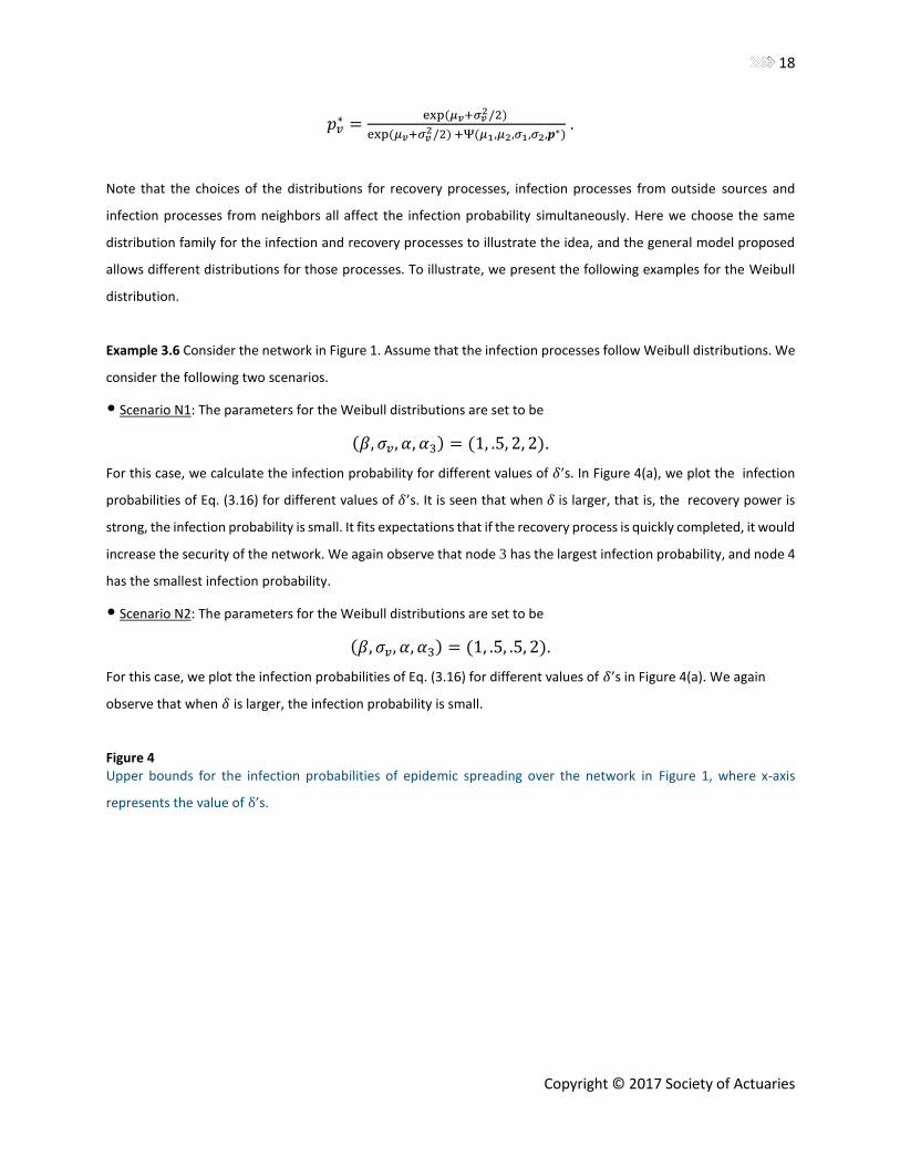
Example 3.6 Consider the network in Figure 1. Assume that the infection processes follow Weibull distributions. We

consider the following two scenarios.

• Scenario N1: The parameters for the Weibull distributions are set to be

(𝛽, 𝜎𝑣, 𝛼, 𝛼3) = (1, .5, 2, 2).

For this case, we calculate the infection probability for different values of 𝛿’s. In Figure 4(a), we plot the infection

probabilities of Eq. (3.16) for different values of 𝛿’s. It is seen that when 𝛿 is larger, that is, the recovery power is

strong, the infection probability is small. It fits expectations that if the recovery process is quickly completed, it would

increase the security of the network. We again observe that node 3 has the largest infection probability, and node 4

has the smallest infection probability.

• Scenario N2: The parameters for the Weibull distributions are set to be

(𝛽, 𝜎𝑣, 𝛼, 𝛼3) = (1, .5, .5, 2).

For this case, we plot the infection probabilities of Eq. (3.16) for different values of 𝛿’s in Figure 4(a). We again

observe that when 𝛿 is larger, the infection probability is small.

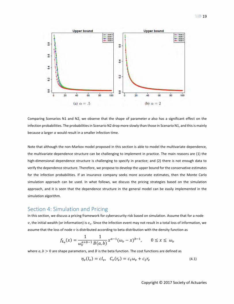
Figure 4 Upper bounds for the infection probabilities of epidemic spreading over the network in Figure 1, where x-axis

represents the value of δ’s.

19


Comparing Scenarios N1 and N2, we observe that the shape of parameter 𝛼 also has a significant effect on the

infection probabilities. The probabilities in Scenario N2 drop more slowly than those in Scenario N1, and this is mainly

because a larger 𝛼 would result in a smaller infection time.

Note that although the non-Markov model proposed in this section is able to model the multivariate dependence,

the multivariate dependence structure can be challenging to implement in practice. The main reasons are (1) the

high-dimensional dependence structure is challenging to specify in practice; and (2) there is not enough data to

verify the dependence structure. Therefore, we propose to develop the upper bound for the conservative estimates

for the infection probabilities. If an insurance company seeks more accurate estimates, then the Monte Carlo

simulation approach can be used. In what follows, we discuss the pricing strategies based on the simulation

approach, and it is seen that the dependence structure in the general model can be easily implemented in the

simulation algorithm.

Section 4: Simulation and Pricing In this section, we discuss a pricing framework for cybersecurity risk based on simulation. Assume that for a node

𝑣, the initial wealth (or information) is 𝑒𝑣. Since the infection event may not result in a total loss of information, we

assume that the loss of node 𝑣 is distributed according to beta distribution with the density function as

𝑓𝑳𝒗(𝑥) =

1

𝜔𝑣𝑎+𝑏−1

1

𝐵(𝑎, 𝑏)𝑥𝑎−1(𝜔𝑣 − 𝑥)𝑏−1, 0 ≤ 𝑥 ≤ 𝜔𝑣

where 𝑎, 𝑏 > 0 are shape parameters, and 𝐵 is the beta function. The cost functions are defined as

𝜂𝑣(𝑙𝑣) = 𝑐𝑙𝑣, 𝐶𝑣(𝑟𝑣) = 𝑐1𝜔𝑣 + 𝑐2𝑟𝑣 (4.1)

20


where 𝑐 means the cost rate due to infection, 𝑐1 represents the cost rate based on the initial value and 𝑐2

represents the cost rate of the recovery process. It is seen that the cost function defined in Eq. (4.1) depends on

not only the duration of downtime but also the wealth of the node.

We study a one-year insurance contract, and two premium principles are considered. The first one is the standard

deviation premium principle:

𝐻(𝑥) = 𝔼[𝑋] + 𝜆√𝑉𝑎𝑟(𝑋) , (4.2)

where 𝜆 > 0 is the risk loading. The second one is the principle of equivalent utility, where the premium 𝐻(𝑋) solves

the equation

𝑢(𝜔𝑣)= 𝔼[𝑢(𝜔𝑣 − 𝑋 + 𝐻(𝑋))] , (4.3)

where 𝑢 is an increasing concave utility of wealth and 𝜔 is the initial wealth. In the rest of the discussion, we consider

the constant relative risk-averse utility function, which is commonly used in the literature [20, 4]:

{

𝜔1−𝛾

1 − 𝛾 , 𝛾 ≠ 1 > 0

log(𝜔) , 𝛾 = 1

,

where 𝛾 is the parameter for the degree of risk aversion. In what follows, we study the pricing strategies based on

the proposed models. The experiment is based on 3,000 Monte Carlo simulations. The parameters for the loss model

are assumed to be (𝑎, 𝑏, 𝑐, 𝑐1, 𝑐2) = (2, 4, .001, .1 × 10−6, .5 × 10−4), and we assume that the initial wealth of

each node is 𝜔𝑣 = 1000 dollars. The simulation algorithm is shown in Algorithm 1.

21


Algorithm 1 allows us to record the evolution of network status during the contract year, and we can calculate the

cumulative loss for each node at any time 𝑡.

4.1 Independent cybersecurity risks In this section, the simulation is based on the assumption that the infection processes are independent. The

quantities we are interested in for each node include (1) the total number of incidents; (2) the infection probability;

and (3) the total loss. The network topology used for the simulation is from Figure 1. We assume that there is no

infection at the beginning, 𝑇 = 0.

4.1.1 Exponential Distribution For this section, we consider the Markov model in Section 3.1. The following two scenarios are considered.

a) Scenario M3: We assume that for any node 𝑣, 𝑣 = 1, ⋯ , 𝑁, the parameters are

(𝛽, 𝜖𝑣, 𝛿𝑣) = (. 2, .5, 1).

Then, it is easy to see that

𝐸(𝑅𝑣) = 1.

Using Eq. (3.15), we can solve the upper bounds for infection probabilities as

(.4833, .4667, .5092, .3737, .4112, .4419, .4429, .4831, .4419, .4094),

and the expected successful infection times can be computed as

22


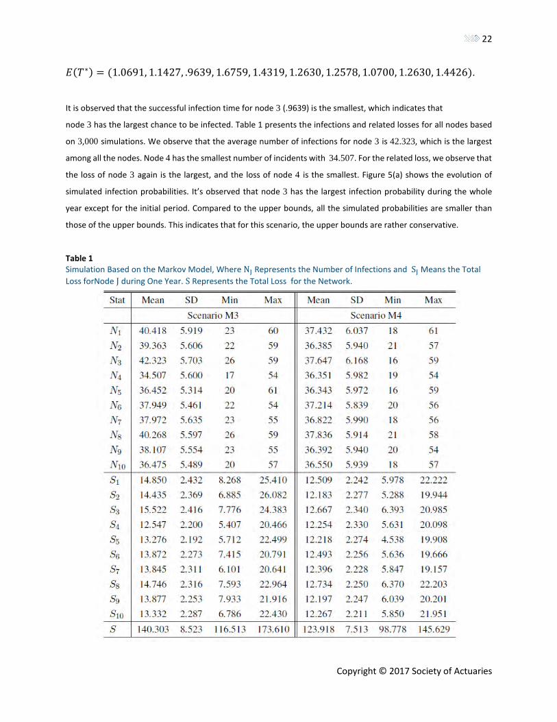
𝐸(𝑇∗) = (1.0691, 1.1427, .9639, 1.6759, 1.4319, 1.2630, 1.2578, 1.0700, 1.2630, 1.4426).

It is observed that the successful infection time for node 3 (.9639) is the smallest, which indicates that

node 3 has the largest chance to be infected. Table 1 presents the infections and related losses for all nodes based

on 3,000 simulations. We observe that the average number of infections for node 3 is 42.323, which is the largest

among all the nodes. Node 4 has the smallest number of incidents with 34.507. For the related loss, we observe that

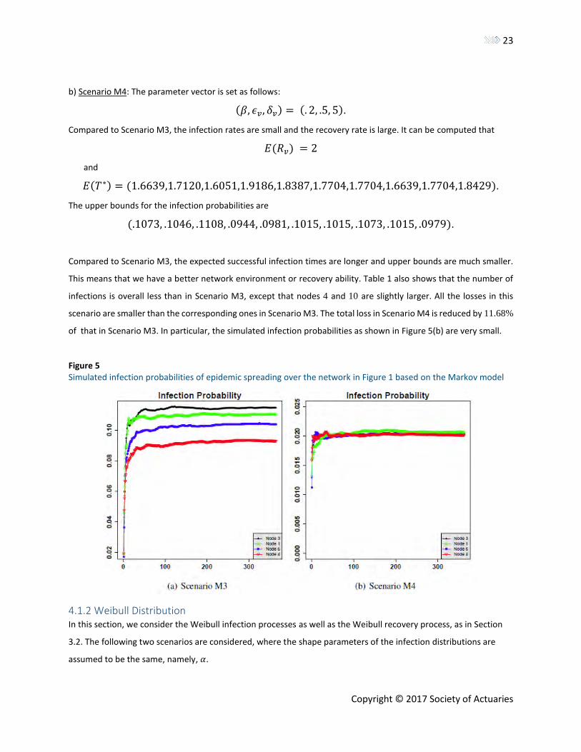
the loss of node 3 again is the largest, and the loss of node 4 is the smallest. Figure 5(a) shows the evolution of

simulated infection probabilities. It’s observed that node 3 has the largest infection probability during the whole

year except for the initial period. Compared to the upper bounds, all the simulated probabilities are smaller than

those of the upper bounds. This indicates that for this scenario, the upper bounds are rather conservative.

Table 1 Simulation Based on the Markov Model, Where NJ Represents the Number of Infections and SJ Means the Total

Loss forNode J during One Year. S Represents the Total Loss for the Network.

23


b) Scenario M4: The parameter vector is set as follows:

(𝛽, 𝜖𝑣, 𝛿𝑣) = (. 2, .5, 5).

Compared to Scenario M3, the infection rates are small and the recovery rate is large. It can be computed that

𝐸(𝑅𝑣) = 2

and

𝐸(𝑇∗) = (1.6639,1.7120,1.6051,1.9186,1.8387,1.7704,1.7704,1.6639,1.7704,1.8429).

The upper bounds for the infection probabilities are

(.1073, .1046, .1108, .0944, .0981, .1015, .1015, .1073, .1015, .0979).

Compared to Scenario M3, the expected successful infection times are longer and upper bounds are much smaller.

This means that we have a better network environment or recovery ability. Table 1 also shows that the number of

infections is overall less than in Scenario M3, except that nodes 4 and 10 are slightly larger. All the losses in this

scenario are smaller than the corresponding ones in Scenario M3. The total loss in Scenario M4 is reduced by 11.68%

of that in Scenario M3. In particular, the simulated infection probabilities as shown in Figure 5(b) are very small.

Figure 5 Simulated infection probabilities of epidemic spreading over the network in Figure 1 based on the Markov model

4.1.2 Weibull Distribution In this section, we consider the Weibull infection processes as well as the Weibull recovery process, as in Section

3.2. The following two scenarios are considered, where the shape parameters of the infection distributions are

assumed to be the same, namely, 𝛼.

24


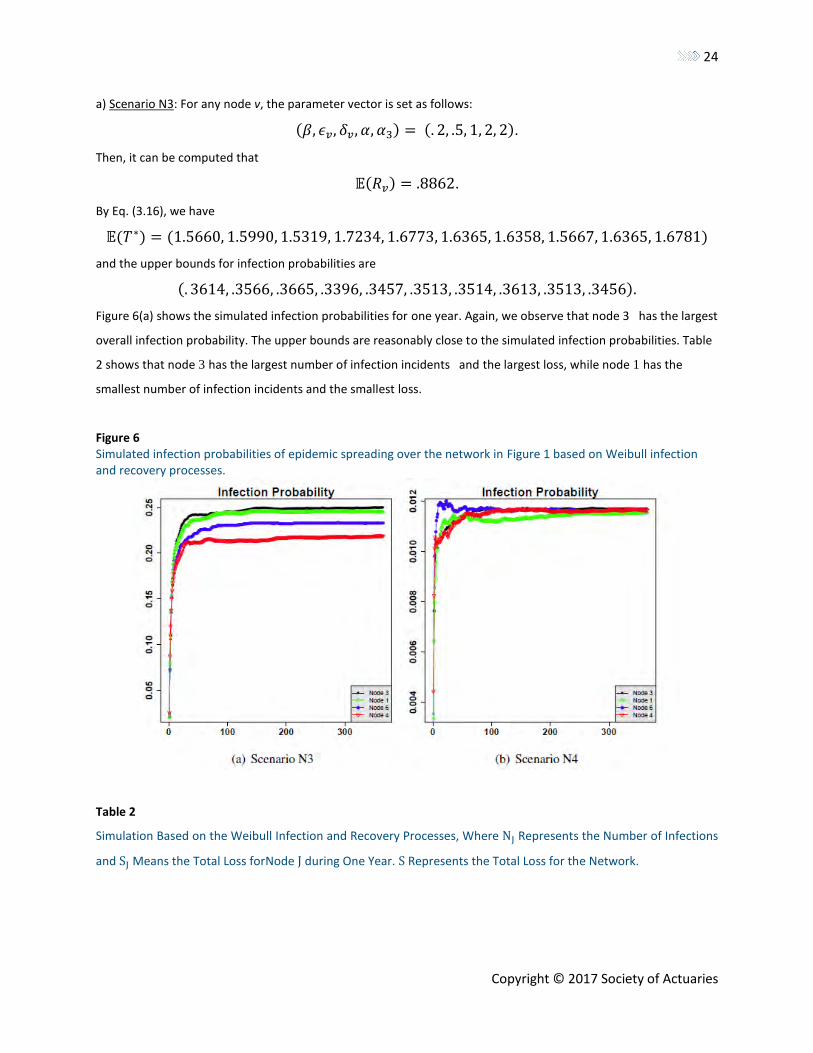
a) Scenario N3: For any node v, the parameter vector is set as follows:

(𝛽, 𝜖𝑣, 𝛿𝑣, 𝛼, 𝛼3) = (. 2, .5, 1, 2, 2).

Then, it can be computed that

𝔼(𝑅𝑣) = .8862.

By Eq. (3.16), we have

𝔼(𝑇∗) = (1.5660, 1.5990, 1.5319, 1.7234, 1.6773, 1.6365, 1.6358, 1.5667, 1.6365, 1.6781)

and the upper bounds for infection probabilities are

(. 3614, .3566, .3665, .3396, .3457, .3513, .3514, .3613, .3513, .3456).

Figure 6(a) shows the simulated infection probabilities for one year. Again, we observe that node 3 has the largest

overall infection probability. The upper bounds are reasonably close to the simulated infection probabilities. Table

2 shows that node 3 has the largest number of infection incidents and the largest loss, while node 1 has the

smallest number of infection incidents and the smallest loss.

Figure 6 Simulated infection probabilities of epidemic spreading over the network in Figure 1 based on Weibull infection and recovery processes.

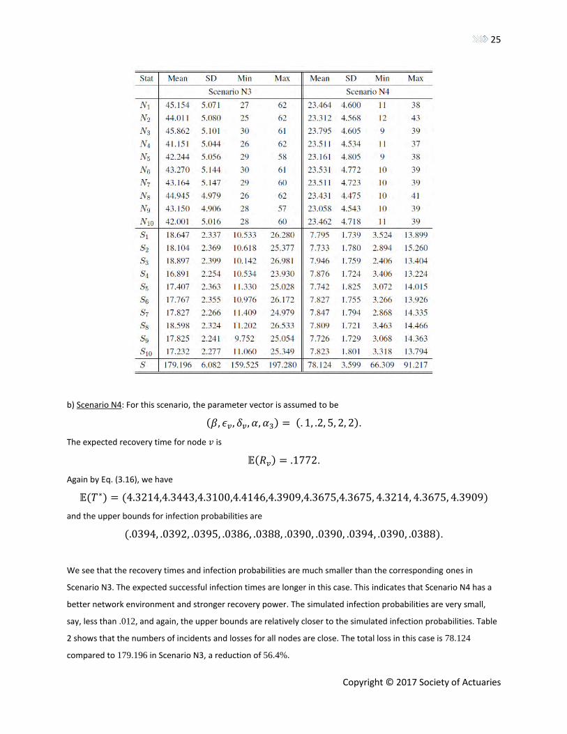
Table 2

Simulation Based on the Weibull Infection and Recovery Processes, Where NJ Represents the Number of Infections

and SJ Means the Total Loss forNode J during One Year. S Represents the Total Loss for the Network.

25


b) Scenario N4: For this scenario, the parameter vector is assumed to be

(𝛽, 𝜖𝑣, 𝛿𝑣, 𝛼, 𝛼3) = (. 1, .2, 5, 2, 2).

The expected recovery time for node 𝑣 is

𝔼(𝑅𝑣) = .1772.

Again by Eq. (3.16), we have

𝔼(𝑇∗) = (4.3214,4.3443,4.3100,4.4146,4.3909,4.3675,4.3675, 4.3214, 4.3675, 4.3909)

and the upper bounds for infection probabilities are

(.0394, .0392, .0395, .0386, .0388, .0390, .0390, .0394, .0390, .0388).

We see that the recovery times and infection probabilities are much smaller than the corresponding ones in

Scenario N3. The expected successful infection times are longer in this case. This indicates that Scenario N4 has a

better network environment and stronger recovery power. The simulated infection probabilities are very small,

say, less than .012, and again, the upper bounds are relatively closer to the simulated infection probabilities. Table

2 shows that the numbers of incidents and losses for all nodes are close. The total loss in this case is 78.124

compared to 179.196 in Scenario N3, a reduction of 56.4%.

26


4.1.3 Log-Normal Distribution In this section, we consider the log-normal infection processes as well as the log-normal recovery process, as in

Section 3.2. The following two scenarios are considered.

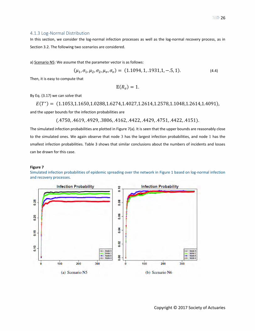
a) Scenario N5: We assume that the parameter vector is as follows:

(𝜇1, 𝜎1, 𝜇2, 𝜎2, 𝜇𝑣, 𝜎𝑣) = (1.1094, 1, .1931,1, −.5, 1). (4.4)

Then, it is easy to compute that

𝔼(𝑅𝑣) = 1.

By Eq. (3.17) we can solve that

𝐸(𝑇∗) = (1.1053,1.1650,1.0288,1.6274,1.4027,1.2614,1.2578,1.1048,1.2614,1.4091),

and the upper bounds for the infection probabilities are

(.4750, .4619, .4929, .3806, .4162, .4422, .4429, .4751, .4422, .4151).

The simulated infection probabilities are plotted in Figure 7(a). It is seen that the upper bounds are reasonably close

to the simulated ones. We again observe that node 3 has the largest infection probabilities, and node 1 has the

smallest infection probabilities. Table 3 shows that similar conclusions about the numbers of incidents and losses

can be drawn for this case.

Figure 7 Simulated infection probabilities of epidemic spreading over the network in Figure 1 based on log-normal infection and recovery processes.

27


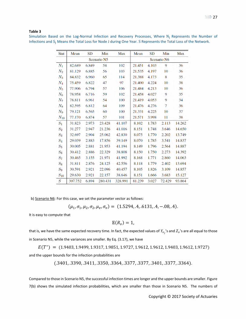
Table 3 Simulation Based on the Log-Normal Infection and Recovery Processes, Where NJ Represents the Number of

Infections and SJ Means the Total Loss for Node J during One Year. S Represents the Total Loss of the Network.

b) Scenario N6: For this case, we set the parameter vector as follows:

(𝜇1, 𝜎1, 𝜇2, 𝜎2, 𝜇𝑣, 𝜎𝑣) = (1.5294, .4, .6131, .4, −.08, .4).

It is easy to compute that

𝔼(𝑅𝑣) = 1,

that is, we have the same expected recovery time. In fact, the expected values of 𝑌𝑣𝑗’s and 𝑍𝑣’s are all equal to those

in Scenario N5, while the variances are smaller. By Eq. (3.17), we have

𝐸(𝑇∗) = (1.9403, 1.9499, 1.9317, 1.9851, 1.9727, 1.9612, 1.9612, 1.9403, 1.9612, 1.9727)

and the upper bounds for the infection probabilities are

(.3401, .3390, .3411, .3350, .3364, .3377, .3377, .3401, .3377, .3364).

Compared to those in Scenario N5, the successful infection times are longer and the upper bounds are smaller. Figure

7(b) shows the simulated infection probabilities, which are smaller than those in Scenario N5. The numbers of

28


incidents and losses for nodes are much less than the corresponding ones in Scenario N5. This indicates that the

smaller variances would lead to less risk. The total loss in Scenario N6 is 81.239 compared to 307.752 in Scenario N5,

a reduction of 73.6%. Therefore, we conclude that larger variances of infection processes result in larger risks.

4.2 Dependent Cybersecurity Risks In this section, we study the dependence effect on the evolution of epidemic spreading and related losses. The

Gaussian copula in Eq. (3.7) and the Clayton copula in Eq. (3.8) are considered in the simulation. For the Gaussian

copula, we consider the cases of using the correlation matrices (3.6) and (3.11), without neighboring effects and

with neighboring effects, respectively. For comparison, we consider the log-normal infection and recovery processes

in what follows.

4.2.1 Gaussian Copula We assume that the parameter vector is as follows:

(𝜇1, 𝜎1, 𝜇2, 𝜎2, 𝜇𝑣, 𝜎𝑣) = (1.1094, 1, .1931, 1, −.5, 1),

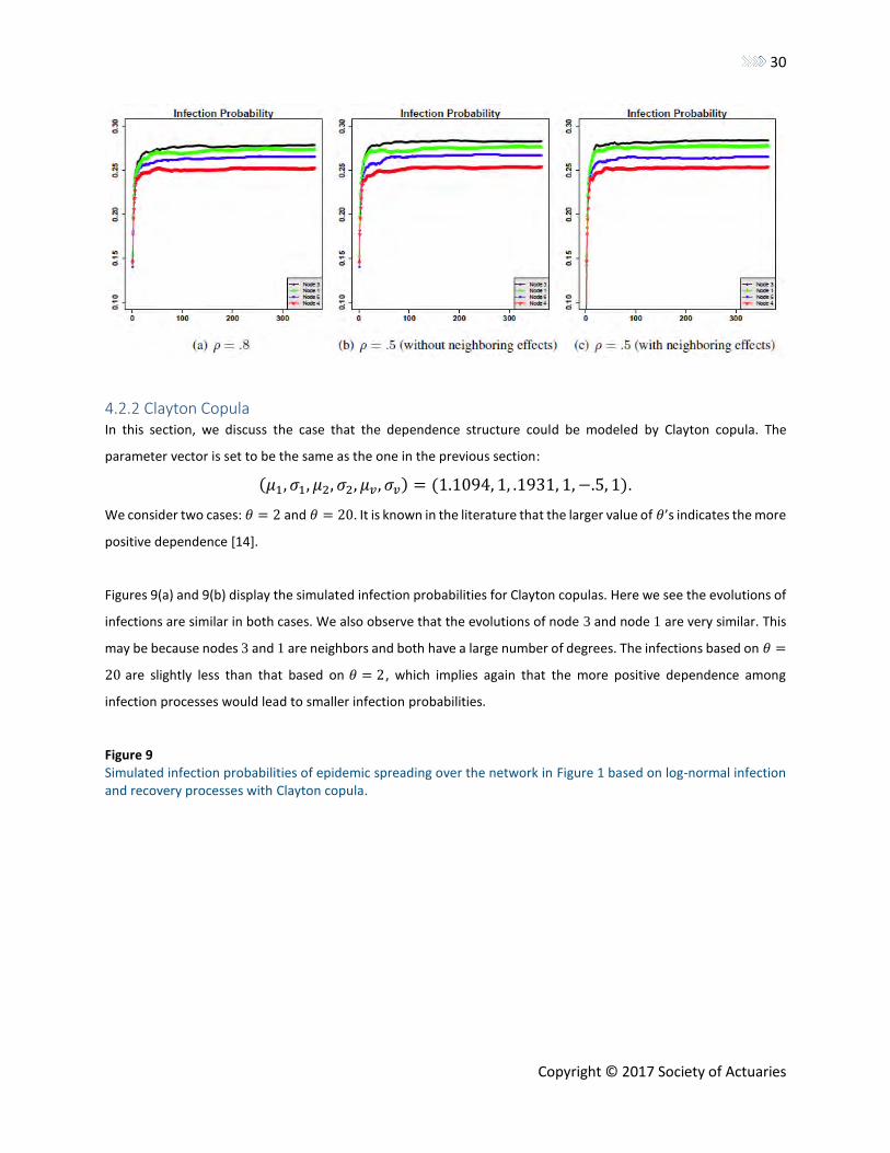
which is the same as that in Scenario N5 in Section 4.1.3. We consider three cases: 𝜌 = .8, 𝜌 = .5 (without

neighboring effects), and 𝜌 = .5 (with neighboring effects). It is known that a larger 𝜌 implies more positive

dependence. Further, the simulated infection probabilities in Figure 8(b) and 8(c) are slightly larger than those in

Figure 8(a), and this indicates that the more positive the dependence, the smaller the infection probabilities. All of

them show that node 3 has the largest overall infection probabilities, and node 4 has the smallest infection

probabilities.

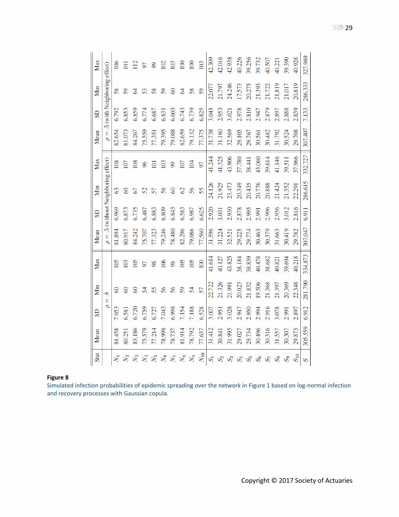
Table 4 shows the numbers of incidents and related losses. We can see that stronger dependence would lead to

fewer overall losses. For example, the total loss for 𝜌 = .8 is 305.559 while the total losses for 𝜌 = .5 are 307.047

and 307.407, respectively. The difference between the two cases of 𝜌 = .5, with and without the neighboring

effects, is very subtle due to the assumed mechanism of the attack spreading process; that is, as we have assumed

throughout the paper, as long as a node is infected, the other nodes will stop attacking it until it recovers. Therefore,

dependence between neighbors plays only a moderate role, as Figure 8(a) and Table 4 have illustrated. A similar

case can also be observed from the next case with Clayton copulas. Nevertheless, it is interesting to compare the

losses in Table 4 to Table 3, and we observe that the independent case (i.e., 𝜌 = 0) has the largest total loss.

Table 4 Simulation Based on the Log-Normal Infection and Recovery Processes with Gaussian Copula, Where NJ Represents

the Number of Infections for Node J during One Year and SJ the Total Loss for Node J during One Year. S Represents

the Total Loss for the Network.

29


Figure 8 Simulated infection probabilities of epidemic spreading over the network in Figure 1 based on log-normal infection and recovery processes with Gaussian copula.

30


4.2.2 Clayton Copula In this section, we discuss the case that the dependence structure could be modeled by Clayton copula. The

parameter vector is set to be the same as the one in the previous section:

(𝜇1, 𝜎1, 𝜇2, 𝜎2, 𝜇𝑣, 𝜎𝑣) = (1.1094, 1, .1931, 1, −.5, 1).

We consider two cases: 𝜃 = 2 and 𝜃 = 20. It is known in the literature that the larger value of 𝜃’s indicates the more

positive dependence [14].

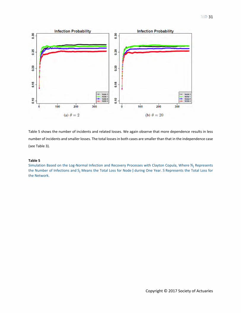
Figures 9(a) and 9(b) display the simulated infection probabilities for Clayton copulas. Here we see the evolutions of

infections are similar in both cases. We also observe that the evolutions of node 3 and node 1 are very similar. This

may be because nodes 3 and 1 are neighbors and both have a large number of degrees. The infections based on 𝜃 =

20 are slightly less than that based on 𝜃 = 2, which implies again that the more positive dependence among

infection processes would lead to smaller infection probabilities.

Figure 9 Simulated infection probabilities of epidemic spreading over the network in Figure 1 based on log-normal infection and recovery processes with Clayton copula.

31


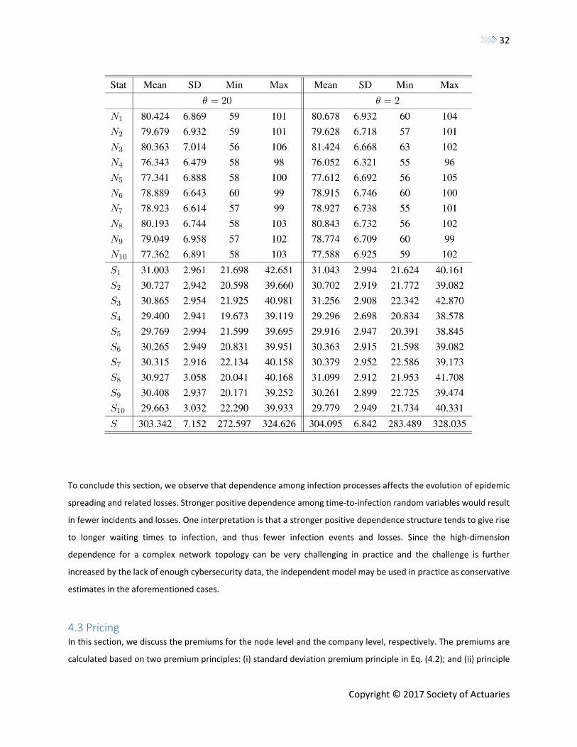
Table 5 shows the number of incidents and related losses. We again observe that more dependence results in less

number of incidents and smaller losses. The total losses in both cases are smaller than that in the independence case

(see Table 3).

Table 5 Simulation Based on the Log-Normal Infection and Recovery Processes with Clayton Copula, Where NJ Represents

the Number of Infections and SJ Means the Total Loss for Node J during One Year. S Represents the Total Loss for

the Network.

32


To conclude this section, we observe that dependence among infection processes affects the evolution of epidemic

spreading and related losses. Stronger positive dependence among time-to-infection random variables would result

in fewer incidents and losses. One interpretation is that a stronger positive dependence structure tends to give rise

to longer waiting times to infection, and thus fewer infection events and losses. Since the high-dimension

dependence for a complex network topology can be very challenging in practice and the challenge is further

increased by the lack of enough cybersecurity data, the independent model may be used in practice as conservative

estimates in the aforementioned cases.

4.3 Pricing In this section, we discuss the premiums for the node level and the company level, respectively. The premiums are

calculated based on two premium principles: (i) standard deviation premium principle in Eq. (4.2); and (ii) principle

33


of equivalent utility in Eq. (4.3). For each principle, we consider three scenarios based on log-normal infection and

recovery processes discussed in the previous sections: (1) independent model in Eq. (4.4); (2) Gaussian dependent

model with 𝜌 = .8; and (3) Clayton dependent model with 𝜃 = 20. For principle (i), 𝜆 = .2, and for principle (ii), 𝛾 =

.8. We assume that the parameter vector is as follows:

(𝜇1, 𝜎1, 𝜇2, 𝜎2, 𝜇𝑣, 𝜎𝑣) = (1.1094, 1, .1931, 1, −.5, 1),

which is the same as that in Scenario N5 in Section 4.1.3.

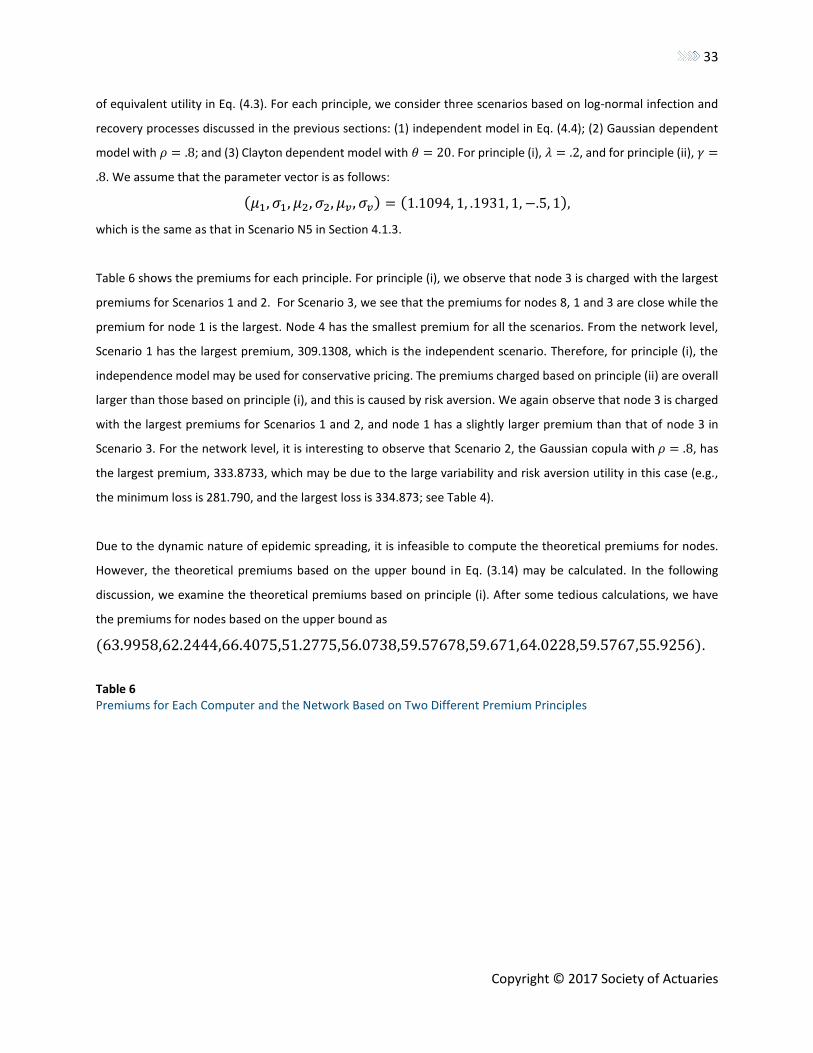
Table 6 shows the premiums for each principle. For principle (i), we observe that node 3 is charged with the largest

premiums for Scenarios 1 and 2. For Scenario 3, we see that the premiums for nodes 8, 1 and 3 are close while the

premium for node 1 is the largest. Node 4 has the smallest premium for all the scenarios. From the network level,

Scenario 1 has the largest premium, 309.1308, which is the independent scenario. Therefore, for principle (i), the

independence model may be used for conservative pricing. The premiums charged based on principle (ii) are overall

larger than those based on principle (i), and this is caused by risk aversion. We again observe that node 3 is charged

with the largest premiums for Scenarios 1 and 2, and node 1 has a slightly larger premium than that of node 3 in

Scenario 3. For the network level, it is interesting to observe that Scenario 2, the Gaussian copula with 𝜌 = .8, has

the largest premium, 333.8733, which may be due to the large variability and risk aversion utility in this case (e.g.,

the minimum loss is 281.790, and the largest loss is 334.873; see Table 4).

Due to the dynamic nature of epidemic spreading, it is infeasible to compute the theoretical premiums for nodes.

However, the theoretical premiums based on the upper bound in Eq. (3.14) may be calculated. In the following

discussion, we examine the theoretical premiums based on principle (i). After some tedious calculations, we have

the premiums for nodes based on the upper bound as

(63.9958,62.2444,66.4075,51.2775,56.0738,59.57678,59.671,64.0228,59.5767,55.9256).

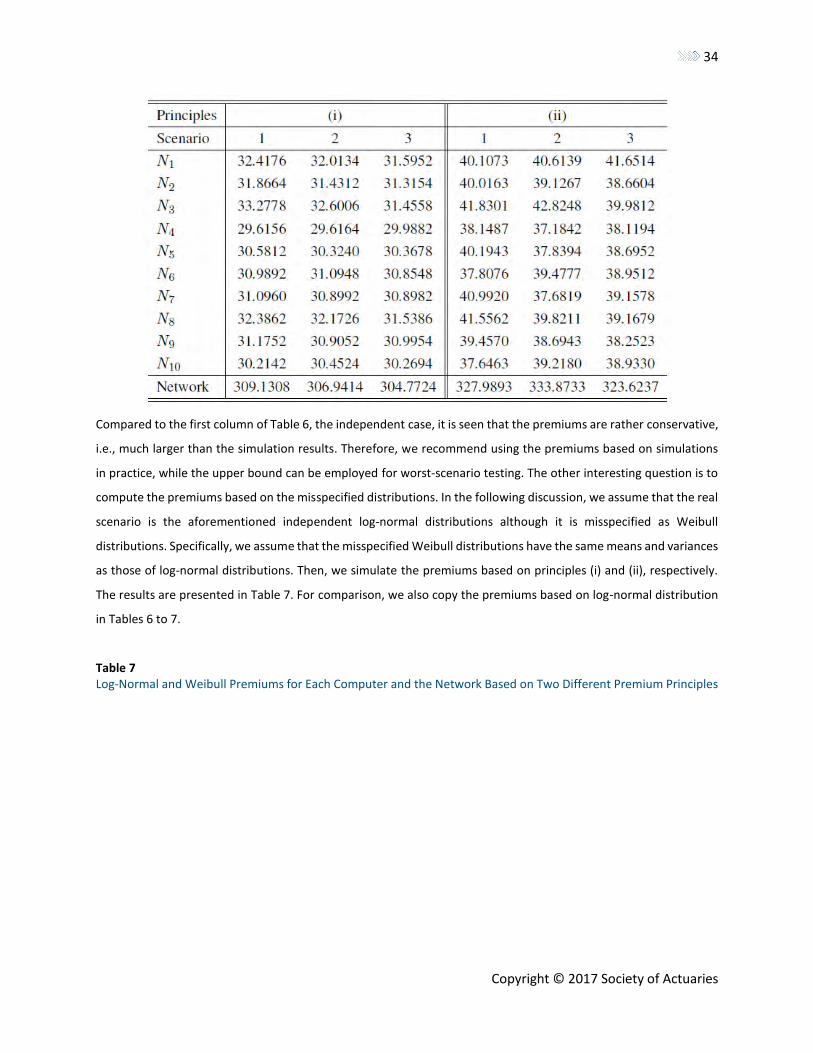
Table 6 Premiums for Each Computer and the Network Based on Two Different Premium Principles

34


Compared to the first column of Table 6, the independent case, it is seen that the premiums are rather conservative,

i.e., much larger than the simulation results. Therefore, we recommend using the premiums based on simulations

in practice, while the upper bound can be employed for worst-scenario testing. The other interesting question is to

compute the premiums based on the misspecified distributions. In the following discussion, we assume that the real

scenario is the aforementioned independent log-normal distributions although it is misspecified as Weibull

distributions. Specifically, we assume that the misspecified Weibull distributions have the same means and variances

as those of log-normal distributions. Then, we simulate the premiums based on principles (i) and (ii), respectively.

The results are presented in Table 7. For comparison, we also copy the premiums based on log-normal distribution

in Tables 6 to 7.

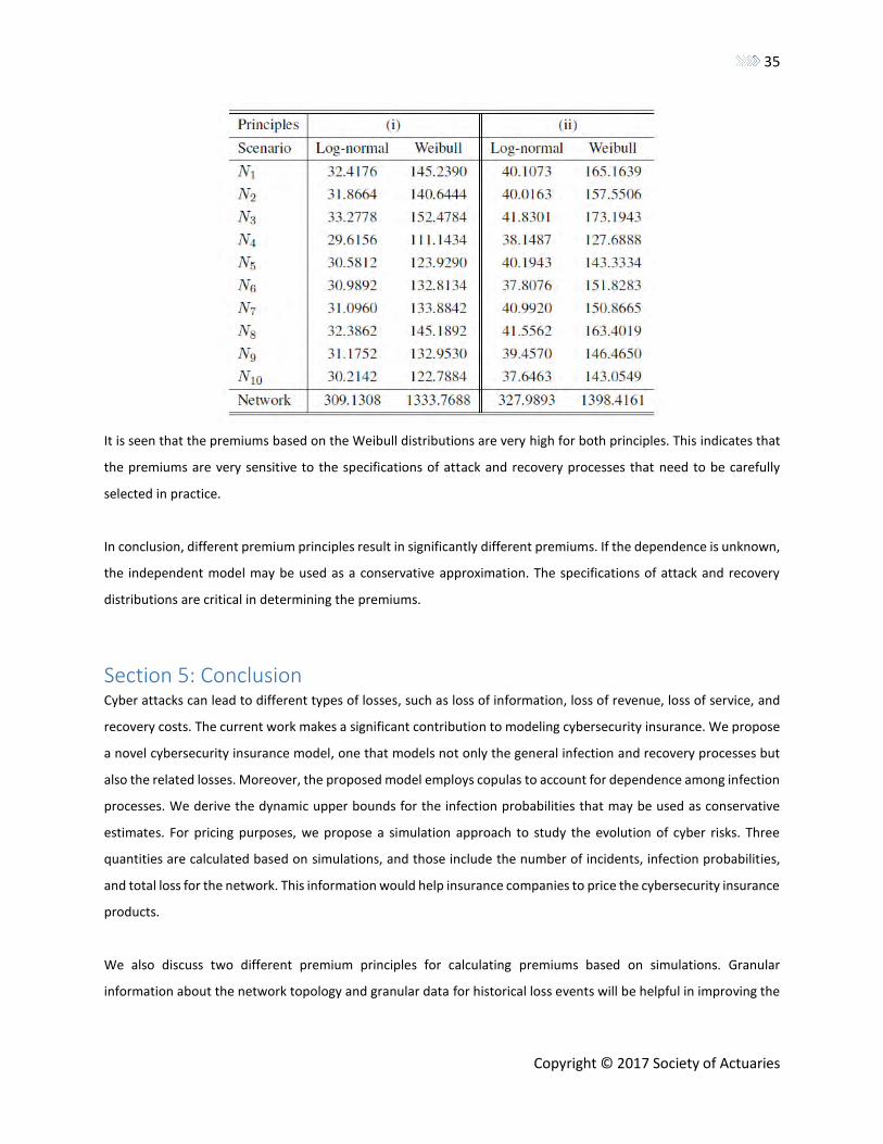
Table 7 Log-Normal and Weibull Premiums for Each Computer and the Network Based on Two Different Premium Principles

35


It is seen that the premiums based on the Weibull distributions are very high for both principles. This indicates that

the premiums are very sensitive to the specifications of attack and recovery processes that need to be carefully

selected in practice.

In conclusion, different premium principles result in significantly different premiums. If the dependence is unknown,

the independent model may be used as a conservative approximation. The specifications of attack and recovery

distributions are critical in determining the premiums.

Section 5: Conclusion Cyber attacks can lead to different types of losses, such as loss of information, loss of revenue, loss of service, and

recovery costs. The current work makes a significant contribution to modeling cybersecurity insurance. We propose

a novel cybersecurity insurance model, one that models not only the general infection and recovery processes but

also the related losses. Moreover, the proposed model employs copulas to account for dependence among infection

processes. We derive the dynamic upper bounds for the infection probabilities that may be used as conservative

estimates. For pricing purposes, we propose a simulation approach to study the evolution of cyber risks. Three

quantities are calculated based on simulations, and those include the number of incidents, infection probabilities,

and total loss for the network. This information would help insurance companies to price the cybersecurity insurance

products.

We also discuss two different premium principles for calculating premiums based on simulations. Granular

information about the network topology and granular data for historical loss events will be helpful in improving the

36


accuracy of rates. Nevertheless, the proposed framework for modeling and pricing of cyber risks for such a network-

based system can also be used as a scoring system for the purpose of internal and external cyber risk management.

The proposed approach can be considered as microlevel modeling of cybersecurity risks. That is, the dynamics of

attack and recovery processes are modeled, and the related losses are simulated. This proposed approach relies on

the underlying stochastic processes and epidemic theory, and it may require a large number of simulations based

on the scale and complexity of the network. Some other interesting future research includes exploration into the

macrolevel modeling of cybersecurity risks. That is, it becomes feasible to use information of network configurations,

network flows, historical cyber incidents, security protocols, and so forth to develop statistical models for modeling

and predicting cybersecurity risks, and, therefore, risk assessments for a large-scale network.

References [1] A. Barrat, M. Barthlemy, and A. Vespignani. Dynamical Processes on Complex Networks. Cambridge: Cambridge

University Press, 2008.

[2] R. S. Betterley. Cyber/privacy insurance market survey: A tough market for larger insureds, but smaller insureds

finding eager insurers. The Betterley Report, June 2016.

[3] R. Bohme and G. Kataria. Models and measures for correlation in cyber-insurance. In Fifth Presented at Workshop

on the Economics of Information Security, University of Cambridge, UK, June 2006.

[4] R. Bohme and G. Schwartz. Modeling cyber-insurance: Towards a unifying framework. In Ninth Presented at

Workshop on the Economics of Information Security, Harvard, June 2010.

[5] E. Cator, R. Van de Bovenkamp, and P. Van Mieghem. Susceptible-infected-susceptible epidemics on networks

with general infection and cure times. Physical Review E, 87(6):062816, 2013.

[6] E. Cator and P. Van Mieghem. Nodal infection in Markovian susceptible-infected-susceptible and susceptible-

infected-removed epidemics on networks are non-negatively correlated. Physical Review E, 89(5):052802, 2014.

[7] E. A. Coddington. An Introduction to Ordinary Differential Equations. North Chelmsford, MA: Courier Corporation,

2012.

[8] US Department of Homeland Security. Cybersecurity insurance. https://www.dhs.gov/cybersecurity-

insurance.

[9] C. Doerr, N. Blenn, and P. Van Mieghem. Log-normal infection times of online information spread. PloS One,

8(5):e64349, 2013.

[10] M. Eling and W. Schnell. What do we know about cyber risk and cyber risk insurance? The Journal of Risk

Finance, 17(5), 2016.

37


[11] L. A. Gordon, M. P. Loeb, and T. Sohail. A framework for using insurance for cyber- risk management.

Communications of the ACM, 46(3):81–85, 2003.

[13] V. S. B. Herath and T. C. Herath. Copula-based actuarial model for pricing cyber-insurance policies. Insurance

Markets and Companies: Analyses and Actuarial Computations, 2:7–20, 2011.

[14] H. Joe. Dependence Modeling with Copulas. Boca Raton, FL: CRC Press, 2014.

[15] S. Karlin. A First Course in Stochastic Processes. Cambridge, MA: Academic Press, 2014.

[16] T. Kosub. Components and challenges of integrated cyber risk management. Zeitschrift fur die gesamte

Versicherungswissenschaft, 104(5):615–634, 2015.

[17] A. Mukhopadhyay, S. Chatterjee, D. Saha, A. Mahanti, and S. K. Sadhukhan. e-Risk management with insurance:

A framework using copula aided Bayesian belief networks. In Proceedings of the 39th Annual Hawaii International

Conference on System Sciences (HICSS’06), vol. 6, 126.1–126.6. Hoboken, NJ: IEEE, 2006.

[18] R. B. Nelsen. An Introduction to Copulas. Vol. 139. New York: Springer Science & Business Media, 2013.

[19] R. Pastor-Satorras, C. Castellano, P. Van Mieghem, and A. Vespignani. Epidemic processes in complex networks.

Reviews of Modern Physics, 87(3):925, 2015.

[20] J. W. Pratt. Risk aversion in the small and in the large. In Foundations of Insurance Economics, 83–98. New York:

Springer, 1992.

[21] S. Ross. Stochastic Processes. Hoboken, NJ: Wiley and Sons, 1996.

[22] G. A. Schwartz and S. S. Sastry. Cyber-insurance framework for large-scale interdependent networks. In

Proceedings of the Third International Conference on High Confidence Networked Systems, 145–154. New York: ACM,

2014.

[23] A. Sklar. Distribution Functions of n dimensions and their margins. Publications de l’Institut de statistique de

l’Universite’ de Paris, 8:229–231, 1959.

[24] P. Van Mieghem and R. Van de Bovenkamp. Non-Markovian infection spread dramatically alters the susceptible-

infected-susceptible epidemic threshold in networks. Physical Review Letters, 110(10):108701, 2013.

[25] P. Van Mieghem. Performance Analysis of Complex Networks and Systems. Cambridge: Cambridge University

Press, 2014.

[26] P. Van Mieghem and E. Cator. Epidemics in networks with nodal self-infection and the epidemic threshold.

Physical Review E, 86(1):016116, 2012.

[27] M. Xu, G. Da, and S. Xu. Cyber epidemic models with dependences. Internet Mathematics, 11(1):62–92, 2015.

[28] M. Xu and S. Xu. An extended stochastic model for quantitative security analysis of networked systems. Internet

Mathematics, 8(3):288–320, 2012.

[29] Z. Yang and J. C. S. Lui. Security adoption and influence of cyber-insurance markets in heterogeneous networks.

Performance Evaluation, 74:1–17, 2014.

38


About The Society of Actuaries The Society of Actuaries (SOA), formed in 1949, is one of the largest actuarial professional organizations in the world, dedicated

to serving more than 27,000 actuarial members and the public in the United States, Canada and worldwide. In line with the SOA

Vision Statement, actuaries act as business leaders who develop and use mathematical models to measure and manage risk in

support of financial security for individuals, organizations and the public.

The SOA supports actuaries and advances knowledge through research and education. As part of its work, the SOA seeks to

inform public policy development and public understanding through research. The SOA aspires to be a trusted source of

objective, data-driven research and analysis with an actuarial perspective for its members, industry, policymakers and the public.

This distinct perspective comes from the SOA as an association of actuaries, who have a rigorous formal education and direct

experience as practitioners as they perform applied research. The SOA also welcomes the opportunity to partner with other

organizations in our work where appropriate.

The SOA has a history of working with public policy makers and regulators in developing historical experience studies and

projection techniques as well as individual reports on health care, retirement and other topics. The SOA’s research is intended to

aid the work of policymakers and regulators and follow certain core principles:

Objectivity: The SOA’s research informs and provides analysis that can be relied upon by other individuals or organizations

involved in public policy discussions. The SOA does not take advocacy positions or lobby specific policy proposals.

Quality: The SOA aspires to the highest ethical and quality standards in all of its research and analysis. Our research process is

overseen by experienced actuaries and nonactuaries from a range of industry sectors and organizations. A rigorous peer-review

process ensures the quality and integrity of our work.

Relevance: The SOA provides timely research on public policy issues. Our research advances actuarial knowledge while providing

critical insights on key policy issues, and thereby provides value to stakeholders and decision makers.

Quantification: The SOA leverages the diverse skill sets of actuaries to provide research and findings that are driven by the best

available data and methods. Actuaries use detailed modeling to analyze financial risk and provide distinct insight and

quantification. Further, actuarial standards require transparency and the disclosure of the assumptions and analytic approach

underlying the work.

Society of Actuaries 475 N. Martingale Road, Suite 600

Schaumburg, Illinois 60173 www.SOA.org

Documents

Cybersecurity Insurance: Modeling and Pricing...has been reiterated in the workshop and roundtable of the US Department of Homeland Security’s (DHS) National Protection and Programs