CVXR: An R Package for Disciplined Convex Optimization · CVXR: An R Package for Disciplined Convex Optimization Anqi Fu, Balasubramanian Narasimhan, and Stephen Boyd Abstract CVXR

CVXR: AN R PACKAGE FOR

DISCIPLINED CONVEX OPTIMIZATION

By

Anqi Fu Balasubramanian Narasimhan

Stephen Boyd

Technical Report No. 2017-14 November 2017

Department of Statistics STANFORD UNIVERSITY

Stanford, California 94305-4065

CVXR: AN R PACKAGE FOR

DISCIPLINED CONVEX OPTIMIZATION

By

Anqi Fu Balasubramanian Narasimhan

Stephen Boyd Stanford University

Technical Report No. 2017-14 November 2017

This research was supported in part by National Institutes of Health grant

1UL1 RR025744.

Department of Statistics STANFORD UNIVERSITY

Stanford, California 94305-4065

http://statistics.stanford.edu

CVXR: An R Package for Disciplined Convex

Optimization

Anqi Fu, Balasubramanian Narasimhan, and Stephen Boyd

Abstract

CVXR is an R package that provides an object-oriented modeling language for convexoptimization, similar to CVX, CVXPY, YALMIP, and Convex.jl. It allows the user toformulate convex optimization problems in a natural mathematical syntax rather thanthe restrictive standard form required by most solvers. The user specifies an objectiveand set of constraints by combining constants, variables, and parameters using a libraryof functions with known mathematical properties. CVXR then applies signed disciplinedconvex programming (DCP) to verify the problem’s convexity. Once verified, the problemis converted into standard conic form using graph implementations and passed to a conesolver such as ECOS or SCS. We demonstrate CVXR’s modeling framework with severalapplications.

Keywords: Convex Optimization, Disciplined Convex Optimization, Optimization, Regres-sion, Penalized Regression, Isotonic Regression, R package CVXR.

1. Introduction

Optimization plays an important role in fitting many statistical models. Some examplesinclude least squares, ridge and lasso regression, isotonic regression, Huber regression, supportvector machines, and sparse inverse covariance estimation. Many R packages exist for solvingfamilies of such problems. Our package, CVXR, solves the much broader class of convexoptimization problems, which encompasses these families and a wide range of other modelsand methods in statistics. Similar systems already exist for MATLAB (Grant and Boyd 2014;Lofberg 2004), Python (Diamond and Boyd 2016), and Julia (Udell, Mohan, Zeng, Hong,Diamond, and Boyd 2014). CVXR brings these capabilities to R, providing a domain-specificlanguage (DSL) that allows users to easily formulate and solve new problems for which customcode does not exist.

As an illustration, suppose we are given X ∈ Rm×n and y ∈ Rm, and we want to solve theordinary least squares (OLS) problem

minimizeβ

∥y −Xβ∥22

with optimization variable β ∈ Rn. This problem has a well-known analytical solution, whichcan be determined via a variety of methods such as glmnet (Friedman, Hastie, and Tibshirani2010). In CVXR, we can solve for β using the code

beta <- Variable(n)

obj <- sum((y - X %*% beta)^2)

2 CVXR: Disciplined Convex Optimization in R

prob <- Problem(Minimize(obj))

result <- solve(prob)

The first line declares our variable, the second line forms our objective function, the thirdline defines the optimization problem, and the last line solves this problem by converting itinto a second-order cone program and sending it to one of CVXR’s solvers. The results areretrieved with

result$value # Optimal objective

result$getValue(beta) # Optimal variables

result$metrics # Runtime metrics

This code runs slower and requires additional set-up at the beginning. So far, it does not looklike progress. However, suppose we add a constraint to our problem:

minimizeβ

∥y −Xβ∥22subject to βj ≤ βj+1, j = 1, . . . , n− 1.

This is a special case of isotonic regression. Now, we can no longer use glmnet for theoptimization. We would need to find another R package tailored to this type of problem orwrite our own custom solver. With CVXR though, we need only add the constraint as asecond argument to the problem:

prob <- Problem(Minimize(obj), list(diff(beta) >= 0))

Our new problem definition includes the coefficient constraint, and a call to solve with theassociated constraint will produce the solution. In addition to the usual results, we can getthe dual variables with

result$getDualValue(constraints(prob)[[1]])

This example demonstrates CVXR’s chief advantage: flexibility. Users can quickly modifyand re-solve a problem, making our package ideal for prototyping new statistical methods.Its syntax is simple and mathematically intuitive. Furthermore, CVXR combines seamlesslywith native R code as well as several popular packages, allowing it to be incorporated easilyinto a larger analytical framework. The user can, for instance, apply resampling techniqueslike the bootstrap to estimate variability, as we show in §3.2.3.DSLs for convex optimization are already widespread on other application platforms. InR, users have access to the packages listed in the CRAN Task View for Optimization andMathematical Programming. Packages like optimx (Nash and Varadhan 2011) and nloptr(Johnson 2008) implement many different algorithms, each with their own strengths andweaknesses. However, most are limited to a subset of the convex problems we handle orrequire analytical details (e.g., the gradient function) for a particular solver. ROI (Hornik,Meyer, Schwendinger, and Theussl 2017) is perhaps the package closest to ours in spirit. Itoffers an object-oriented framework for defining optimization problems, but still requires usersto explicitly identify the type of every objective and constraint, whereas CVXR manages thisprocess automatically.

Anqi Fu, Balasubramanian Narasimhan, Stephen Boyd 3

In the next section, we provide a brief mathematical overview of convex optimization. Inter-ested readers can find a full treatment in Boyd and Vandenberghe (2004). Then we give aseries of examples ranging from basic regression models to semidefinite programming, whichdemonstrate the simplicity of problem construction in CVXR. Finally, we describe the imple-mentation details before concluding. Our package and the example code for this paper areavailable on CRAN and the official CVXR site.

2. Disciplined Convex Optimization

The general convex optimization problem is of the form

minimizev

f0(v)

subject to fi(v) ≤ 0, i = 1, . . . ,MAv = b,

where v ∈ Rn is our variable of interest, and A ∈ Rm×n and b ∈ Rn are constants describingour linear equality constraints. The objective and inequality constraint functions f0, . . . , fMare convex, i.e., they are functions fi : R

n → R that satisfy

fi(θu+ (1− θ)v) ≤ θfi(u) + (1− θ)fi(v)

for all u, v ∈ Rn and θ ∈ [0, 1]. This class of problems arises in a variety of fields, includingmachine learning and statistics.

A number of efficient algorithms exist for solving convex problems (Wright 1997; Boyd, Parikh,Chu, Peleato, and Eckstein 2011; Andersen, Dahl, Liu, and Vandenberghe 2011; Skajaa andYe 2015). However, it is unnecessary for the CVXR user to know the operational details ofthese algorithms. CVXR provides a DSL that allows the user to specify the problem in anatural mathematical syntax. This specification is automatically converted into the standardform ingested by a generic convex solver. See §4 for more on this process.

In general, it can be difficult to determine whether an optimization problem is convex. Wefollow an approach called disciplined convex programming (DCP) (Grant, Boyd, and Ye 2006)to define problems using a library of basic functions (atoms), whose properties like curvature,monotonicity, and sign are known. Adhering to the DCP rule,

f(g1, . . . , gk) is convex if f is convex and for each i = 1, . . . , k, either

• gi is affine,

• gi is convex and f is increasing in argument i, or

• gi is concave and f is decreasing in argument i,

we combine these atoms such that the resulting problem is convex by construction. Users willneed to become familiar with this rule if they wish to define complex problems.

The library of available atoms is provided in the documentation. It covers an extensive arrayof functions, enabling any user to model and solve a wide variety of sophisticated optimizationproblems. In the next section, we provide sample code for just a few of these problems, manyof which are cumbersome or impossible to solve with other R packages.

https://CRAN.R-project.org/package=CVXR

https://cvxr.rbind.io


3. Examples

In the following examples, we are given a dataset (xi, yi) for i = 1, . . . ,m, where xi ∈ Rn andyi ∈ R. We represent these observations in matrix form as X ∈ Rm×n with stacked rows xTiand y ∈ Rm. Generally, we assume that m > n.

3.1. Regression

Robust (Huber) Regression

In §1, we saw an example of OLS in CVXR. While least squares is a popular regression model,one of its flaws is its high sensitivity to outliers. A single outlier that falls outside the tailsof the normal distribution can drastically alter the resulting coefficients, skewing the fit onthe other data points. For a more robust model, we can fit a Huber regression (Huber 1964)instead by solving

minimizeβ

∑mi=1 ϕ(yi − xTi β)

for variable β ∈ Rn, where the loss is the Huber function with threshold M > 0,

ϕ(u) =

{u2 if |u| ≤ M

2Mu−M2 if |u| > M.

This function is identical to the least squares penalty for small residuals, but on large residuals,its penalty is lower and increases linearly rather than quadratically. It is thus more forgivingof outliers.

In CVXR, the code for this problem is

beta <- Variable(n)

obj <- sum(huber(y - X %*% beta, M))



Note the similarity to the OLS code. As before, the first line instantiates the n-dimensionaloptimization variable, and the second line defines the objective function by combining thisvariable with our data using CVXR’s library of atoms. The only difference this time is we callthe huber atom on the residuals with threshold M, which we assume has been set to a positivescalar constant. Our package provides many such atoms to simplify problem definition forthe user.

Quantile Regression

Another variation on least squares is quantile regression (Koenker 2005). The loss is the tiltedl1 function,

ϕ(u) = τ max(u, 0)− (1− τ)max(−u, 0) =1

2|u|+

(τ − 1

2

)u,

where τ ∈ (0, 1) specifies the quantile. The problem as before is to minimize the total residualloss. This model is commonly used in ecology, healthcare, and other fields where the mean


alone is not enough to capture complex relationships between variables. CVXR allows us tocreate a function to represent the loss and integrate it seamlessly into the problem definition,as illustrated below.

quant_loss <- function(u, tau) { 0.5*abs(u) + (tau - 0.5)*u }

obj <- sum(quant_loss(y - X %*% beta, t))



Here t is the user-defined quantile parameter. We do not need to create a new Variable

object, since we can reuse beta from the previous example.

Censored Regression

Data collected from an experimental study is sometimes censored, so that only partial infor-mation is known about a subset of observations. For instance, when measuring the lifespanof mice, we may find a number of subjects live beyond the duration of the project. Thus, allwe know is the lower bound on their lifespan. This right censoring can be incorporated intoa regression model via convex optimization.

Suppose that only K of our observations (xi, yi) are fully observed, and the remaining arecensored such that we observe xi, but only know yi ≥ D for i = K + 1, . . . ,m and someconstant D ∈ R. We can build an OLS model using the uncensored data, restricting thefitted values yi = xTi β to lie above D for the censored observations:

minimizeβ

∑Ki=1(yi − xTi β)

2

subject to xTi β ≥ D, i = K + 1, . . . ,m.

This avoids the bias introduced by standard OLS, while still utilizing all of the data pointsin the regression. The constraint requires only one more line in CVXR.

beta <- Variable(n)

obj <- sum((y[1:K] - X[1:K,] %*% beta)^2)

constr <- list(X[(K+1):m,] %*% beta >= D)

prob <- Problem(Minimize(obj), constr)


We can just as easily accommodate left censoring, interval censoring, and other loss functionswith minor changes to the code above.

Elastic Net Regularization

Often in applications, we encounter problems that require regularization to prevent overfitting,introduce sparsity, facilitate variable selection, or impose prior distributions on parameters.Two of the most common regularization functions are the l1-norm and squared l2-norm,combined in the elastic net regression model (H. Zou 2005; Friedman et al. 2010),

minimizeβ

12m∥y −Xβ∥22 + λ(1−α

2 ∥β∥22 + α∥β∥1).


Here λ ≥ 0 is the overall regularization weight and α ∈ [0, 1] controls the relative l1 versussquared l2 penalty. Thus, this model encompasses both ridge (α = 0) and lasso (α = 1)regression.

To solve this problem in CVXR, we first define a function that calculates the regularizationterm given the variable and penalty weights.

elastic_reg <- function(beta, lambda = 0, alpha = 0) {

ridge <- (1 - alpha) * sum(beta^2)

lasso <- alpha * p_norm(beta, 1)

lambda * (lasso + ridge)

}

Then, we add it to the scaled least squares loss.

loss <- sum((y - X %*% beta)^2)/(2*m)

obj <- loss + elastic_reg(beta, lambda, alpha)



The advantage of this modular approach is that we can easily incorporate elastic net regu-larization into other regression models. For instance, if we wanted to run regularized Huberregression, CVXR allows us to reuse the above code with just a single changed line,

loss <- huber(y - X %*% beta, M)

Logistic Regression

Suppose now that yi ∈ {0, 1} is a binary class indicator. One of the most popular methodsfor binary classification is logistic regression (Cox 1958; Freedman 2009). We model theconditional response as y|x ∼ Bernoulli(gβ(x)), where gβ(x) =

1

1+e−xT βis the logistic function,

and maximize the log-likelihood function, yielding the optimization problem

maximizeβ

∑mi=1{yi log(gβ(xi)) + (1− yi) log(1− gβ(xi))}.

CVXR provides the logistic atom as a shortcut for f(z) = log(1 + ez), so our problem issuccinctly expressed as

obj <- -sum(logistic(-X[y == 0,] %*% beta)) - sum(logistic(X[y == 1,] %*% beta))

prob <- Problem(Maximize(obj))


The user may be tempted to type log(1 + exp(X %*% beta)) as in conventional R syntax.However, this representation of f(z) violates the DCP composition rule, so the CVXR parserwill reject the problem even though the objective is convex. Users who wish to employa function that is convex, but not DCP compliant should check the documentation for acustom atom or consider a different formulation.

We can retrieve the optimal objective and variables just like in OLS. More interestingly,we can evaluate various functions of these variables as well by passing them directly intoresult$getValue. For instance, the log-odds are


log_odds <- result$getValue(X %*% beta)

This coincides with the ratio we get from computing the probabilities directly:

beta_res <- result$getValue(beta)

y_probs <- 1/(1 + exp(-X %*% beta_res))

log(y_probs/(1 - y_probs))

Many other classification methods fit into the convex framework. For example, the supportvector classifier is the solution of a l2-norm minimization problem with linear constraints,which we have already shown how to model. Support vector machines are a straightforwardextension. The multinomial distribution can be used to predict multiple classes, and esti-mation via maximum likelihood produces a convex problem. To each of these methods, wecan easily add new penalties, variables, and constraints in CVXR, allowing us to adapt to aspecific dataset or environment.

Sparse Inverse Covariance Estimation

Assume we are given i.i.d. observations xi ∼ N(0,Σ) for i = 1, . . . ,m, and the covariancematrix Σ ∈ Sn

+, the set of symmetric positive semidefinite matrices, has a sparse inverseS = Σ−1. Let Q = 1

m−1

∑mi=1(xi− x)(xi− x)T be our sample covariance. One way to estimate

Σ is to maximize the log-likelihood with the prior knowledge that S is sparse (Friedman,Hastie, and Tibshirani 2008), which amounts to the optimization problem

maximizeS

log det(S)− tr(SQ)

subject to S ∈ Sn+,

∑ni=1

∑nj=1 |Sij | ≤ α.

The parameter α ≥ 0 controls the degree of sparsity. Our problem is convex, so we can solveit with

S <- Semidef(n)

obj <- log_det(S) - matrix_trace(S %*% Q)

constr <- list(sum(abs(S)) <= alpha)

prob <- Problem(Maximize(obj), constr)


The Semidef constructor restricts S to the positive semidefinite cone. In our objective, weuse CVXR functions for the log-determinant and trace. The expression matrix_trace(S

%*% Q) is equivalent to sum(diag(S %*% Q)), but the former is preferred because it is moreefficient than making nested function calls. However, a standalone atom does not exist forthe determinant, so we cannot replace log_det(S) with log(det(S)) since det is undefinedfor a Semidef object.

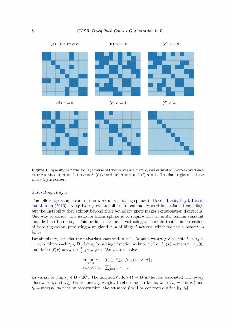
Figure 1 depicts the solutions for a particular dataset withm = 1000, n = 10, and S containing26% non-zero entries represented by the black squares in the top left image. The sparsityof our inverse covariance estimate decreases for higher α, so that when α = 1, most of theoff-diagonal entries are zero, while if α = 10, over half the matrix is dense. At α = 4, weachieve the true percentage of non-zeros.


(a) True Inverse (b) α = 10 (c) α = 8

(d) α = 6 (e) α = 4 (f) α = 1

Figure 1: Sparsity patterns for (a) inverse of true covariance matrix, and estimated inverse covariancematrices with (b) α = 10, (c) α = 8, (d) α = 6, (e) α = 4, and (f) α = 1. The dark regions indicatewhere Sij is nonzero.

Saturating Hinges

The following example comes from work on saturating splines in Boyd, Hastie, Boyd, Recht,and Jordan (2016). Adaptive regression splines are commonly used in statistical modeling,but the instability they exhibit beyond their boundary knots makes extrapolation dangerous.One way to correct this issue for linear splines is to require they saturate: remain constantoutside their boundary. This problem can be solved using a heuristic that is an extensionof lasso regression, producing a weighted sum of hinge functions, which we call a saturatinghinge.

For simplicity, consider the univariate case with n = 1. Assume we are given knots t1 < t2 <· · · < tk where each tj ∈ R. Let hj be a hinge function at knot tj , i.e., hj(x) = max(x− tj , 0),

and define f(x) = w0 +∑k

j=1wjhj(x). We want to solve

minimizew0,w

∑mi=1 ℓ(yi, f(xi)) + λ∥w∥1

subject to∑k

j=1wj = 0

for variables (w0, w) ∈ R×Rk. The function ℓ : R×R → R is the loss associated with everyobservation, and λ ≥ 0 is the penalty weight. In choosing our knots, we set t1 = min(xi) andtk = max(xi) so that by construction, the estimate f will be constant outside [t1, tk].


We demonstrate this technique on the bone density data for female patients from Hastie,Tibshirani, and Friedman (2001, §5.4). There are a total of m = 259 observations. Ourresponse yi is the change in spinal bone density between two visits, and our predictor xi isthe patient’s age. We select k = 10 knots about evenly spaced across the range of X and fita saturating hinge with squared error loss ℓ(yi, f(xi)) = (yi − f(xi))

2.

In R, we first define the estimation and loss functions:

f_est <- function(x, knots, w0, w) {

hinges <- sapply(knots, function(t) { pmax(x - t, 0) })

w0 + hinges %*% w

}

loss_obs <- function(y, f) { (y - f)^2 }

This allows us to easily test different losses and knot locations later. The rest of the set-up issimilar to previous examples. We assume that knots is a R vector representing (t1, . . . , tk).

w0 <- Variable()

w <- Variable(k)

loss <- sum(loss_obs(y, f_est(X, knots, w0, w)))

reg <- lambda * p_norm(w, 1)

obj <- loss + reg

constr <- list(sum(w) == 0)



The optimal weights are retrieved using separate calls, as shown below.

w0s <- result$getValue(w0)

ws <- result$getValue(w)

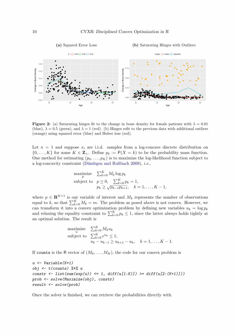
We plot the fitted saturating hinges in Figure 2a. As expected, when λ increases, the splineexhibits less variation and grows flatter outside its boundaries. The squared error loss workswell in this case, but as we saw in §3.1.1, the Huber loss is preferred when the dataset containslarge outliers. We can change the loss function by simply redefining

loss_obs <- function(y, f, M) { huber(y - f, M) }

and passing an extra threshold parameter in when initializing loss. In Figure 2b, we haveadded 50 randomly generated outliers to the bone density data and plotted the re-fittedsaturating hinges. For a Huber loss with M = 0.01, the resulting spline is fairly smooth andfollows the shape of the original data, as opposed to the spline using squared error loss, whichis biased upwards by a significant amount.

3.2. Nonparametric Estimation

Log-Concave Distribution Estimation


(a) Squared Error Loss

●

●

●

●

●●

●

●

●

●

●

●

●

●

●

●

●

●

●

●

●

●

●

●

●

●

●

●●

●

●

●

●

●

●

●

●

●

●

●

●

●

●

●●

●

●

●●

●

●

●

●

●

●

●

●

●

●

●

●

●

●

●

●

●

●

●

●

●

●

●

●

●

●

●

●

●●

●

●

●●

●

●●

●●

●

●

●

●

●

●

●●

●

●

●

●

●●

●

●●

●

●

●●

●

●

●●●

●

●

●

●

●

●●●

●

●

●

●

●

●

●

●

●

●

●●

●

●

●●

●

●

●

●

●

●

●

●

●

●

●

●

●

●

●

●●●

●

●

●

●

●

●

●

●

●

●

●

●

●●

●

●●

●

●

●

●●●

●

●

●●

●

●●

●

●

●

●

●●

●●

●

●●

●

●

● ●

●●

●

●

●

●●

●

●●●

●●●

●

●●

●●

●

●

●

●

●

●

●

●●

●

●

●

●

●●

●

●

●

●●

●

●

●

●

●●●

●

●

●●

●

●

●●

●

●

● ●

−0.05

0.00

0.05

0.10

0.15

0.20

10 15 20 25

Age

Cha

nge

in B

one

Den

sity

λ 1.00 0.50 0.01

(b) Saturating Hinges with Outliers

●

●

●●

●●

●

●

●

●

●

●

●

●

●●●

●

●

●

●

●

●

●

●

●

●●●

●

●

●

●

●

●●

●

●●

●●

●

●●●●

●

●●

●

●●

●●

●

●

●

●

●

●●

●

●●

●

●●

●

●●

●●●

●

●

●

●

●●

●

●

●●●●●●●

●●

●

●

●●●●

●●●

●●●

●

●●

●

●

●●●

●●●●●●●

●●●●●●●●

●

●●●

●

●●

●●●●●●●●●●

●

●

●

●

●●●●●●●●●●●●●●●

●●

●

●●●●●●

●

● ●●●●

●●●●●●●●●●

●●●

●●●

●●●●●

●

●● ●

●●●●●

●●●●●●●●●● ●●

●●●●●●

●●

●

●●●●

●

●●●

●●●●●●

●●

●●●●

●

●●●

●●●●●

●

● ●

●

●

●

●

●●

●

●

●

●

●

●

●

●

●

●

●

●

●

●

●

●

●●

●

●●

●

●

●

●

●

●

●

●

●

●

●

●

●

●

●

●

●

● ●

●●

●

●

0.00

0.25

0.50

0.75

10 15 20 25

Age

Cha

nge

in B

one

Den

sity

Loss Huber Squared

Figure 2: (a) Saturating hinges fit to the change in bone density for female patients with λ = 0.01(blue), λ = 0.5 (green), and λ = 1 (red). (b) Hinges refit to the previous data with additional outliers(orange) using squared error (blue) and Huber loss (red).

Let n = 1 and suppose xi are i.i.d. samples from a log-concave discrete distribution on{0, . . . ,K} for some K ∈ Z+. Define pk := P(X = k) to be the probability mass function.One method for estimating (p0, . . . , pK) is to maximize the log-likelihood function subject toa log-concavity constraint (Dumbgen and Rufibach 2009), i.e.,

maximizep

∑Kk=0Mk log pk

subject to p ≥ 0,∑K

k=0 pk = 1,pk ≥ √

pk−1pk+1, k = 1, . . . ,K − 1,

where p ∈ RK+1 is our variable of interest and Mk represents the number of observationsequal to k, so that

∑Kk=0Mk = m. The problem as posed above is not convex. However, we

can transform it into a convex optimization problem by defining new variables uk = log pkand relaxing the equality constraint to

∑Kk=0 pk ≤ 1, since the latter always holds tightly at

an optimal solution. The result is

maximizeu

∑Kk=0Mkuk

subject to∑K

k=0 euk ≤ 1,

uk − uk−1 ≥ uk+1 − uk, k = 1, . . . ,K − 1.

If counts is the R vector of (M0, . . . ,MK), the code for our convex problem is

u <- Variable(K+1)

obj <- t(counts) %*% u

constr <- list(sum(exp(u)) <= 1, diff(u[1:K)]) >= diff(u[2:(K+1)]))

prob <- solve(Maximize(obj), constr)


Once the solver is finished, we can retrieve the probabilities directly with


(a) Probability Mass Function

0.000

0.005

0.010

0.015

0.020

0 25 50 75 100

x

Est

imat

e

Type True Empirical Optimal

(b) Cumulative Distribution Function

0.00

0.25

0.50

0.75

1.00

0 25 50 75 100

x

Est

imat

e

Type True Empirical Optimal

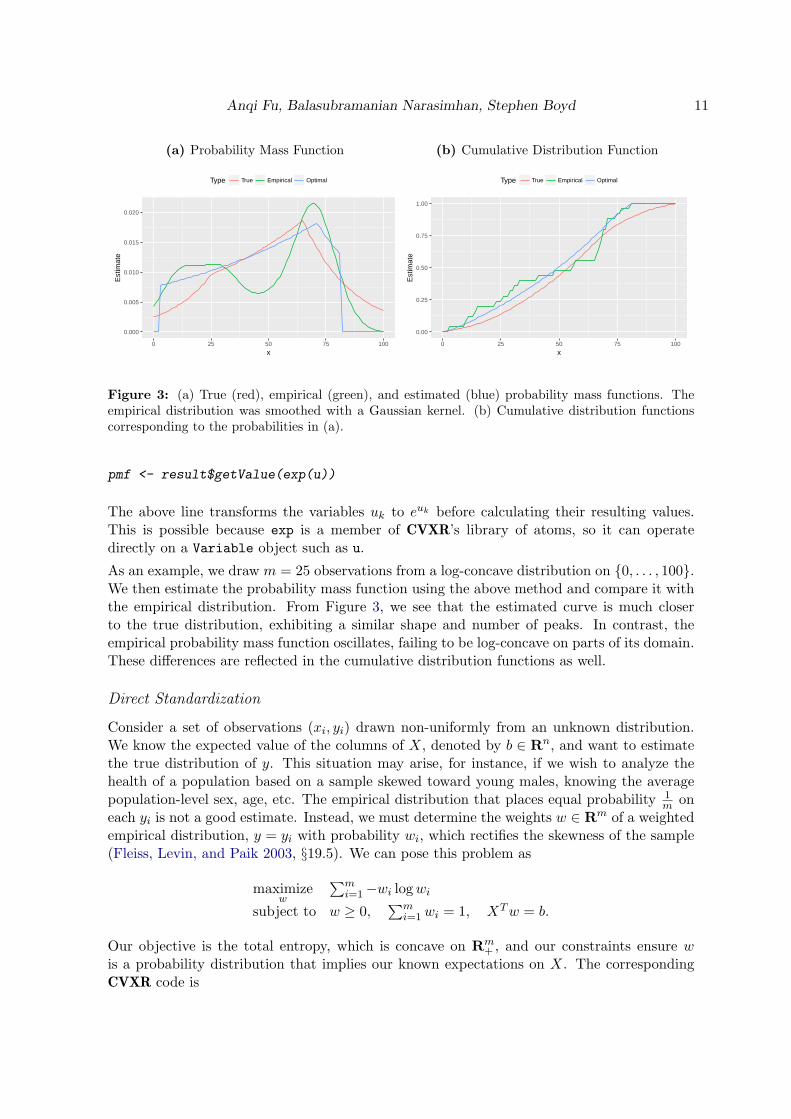
Figure 3: (a) True (red), empirical (green), and estimated (blue) probability mass functions. Theempirical distribution was smoothed with a Gaussian kernel. (b) Cumulative distribution functionscorresponding to the probabilities in (a).

pmf <- result$getValue(exp(u))

The above line transforms the variables uk to euk before calculating their resulting values.This is possible because exp is a member of CVXR’s library of atoms, so it can operatedirectly on a Variable object such as u.

As an example, we draw m = 25 observations from a log-concave distribution on {0, . . . , 100}.We then estimate the probability mass function using the above method and compare it withthe empirical distribution. From Figure 3, we see that the estimated curve is much closerto the true distribution, exhibiting a similar shape and number of peaks. In contrast, theempirical probability mass function oscillates, failing to be log-concave on parts of its domain.These differences are reflected in the cumulative distribution functions as well.

Direct Standardization

Consider a set of observations (xi, yi) drawn non-uniformly from an unknown distribution.We know the expected value of the columns of X, denoted by b ∈ Rn, and want to estimatethe true distribution of y. This situation may arise, for instance, if we wish to analyze thehealth of a population based on a sample skewed toward young males, knowing the averagepopulation-level sex, age, etc. The empirical distribution that places equal probability 1

m oneach yi is not a good estimate. Instead, we must determine the weights w ∈ Rm of a weightedempirical distribution, y = yi with probability wi, which rectifies the skewness of the sample(Fleiss, Levin, and Paik 2003, §19.5). We can pose this problem as

maximizew

∑mi=1−wi logwi

subject to w ≥ 0,∑m

i=1wi = 1, XTw = b.

Our objective is the total entropy, which is concave on Rm+ , and our constraints ensure w

is a probability distribution that implies our known expectations on X. The correspondingCVXR code is


w <- Variable(m)

obj <- sum(entr(w))

constr <- list(w >= 0, sum(w) == 1, t(X) %*% w == b)



(a) Probability Distribution Function

0.00

0.05

0.10

0.15

0 5 10 15

x

Est

imat

e

Type True Sample Weighted

(b) Cumulative Distribution Function

0.00

0.25

0.50

0.75

1.00

0 5 10

x

Est

imat

e

Type True Sample Weighted

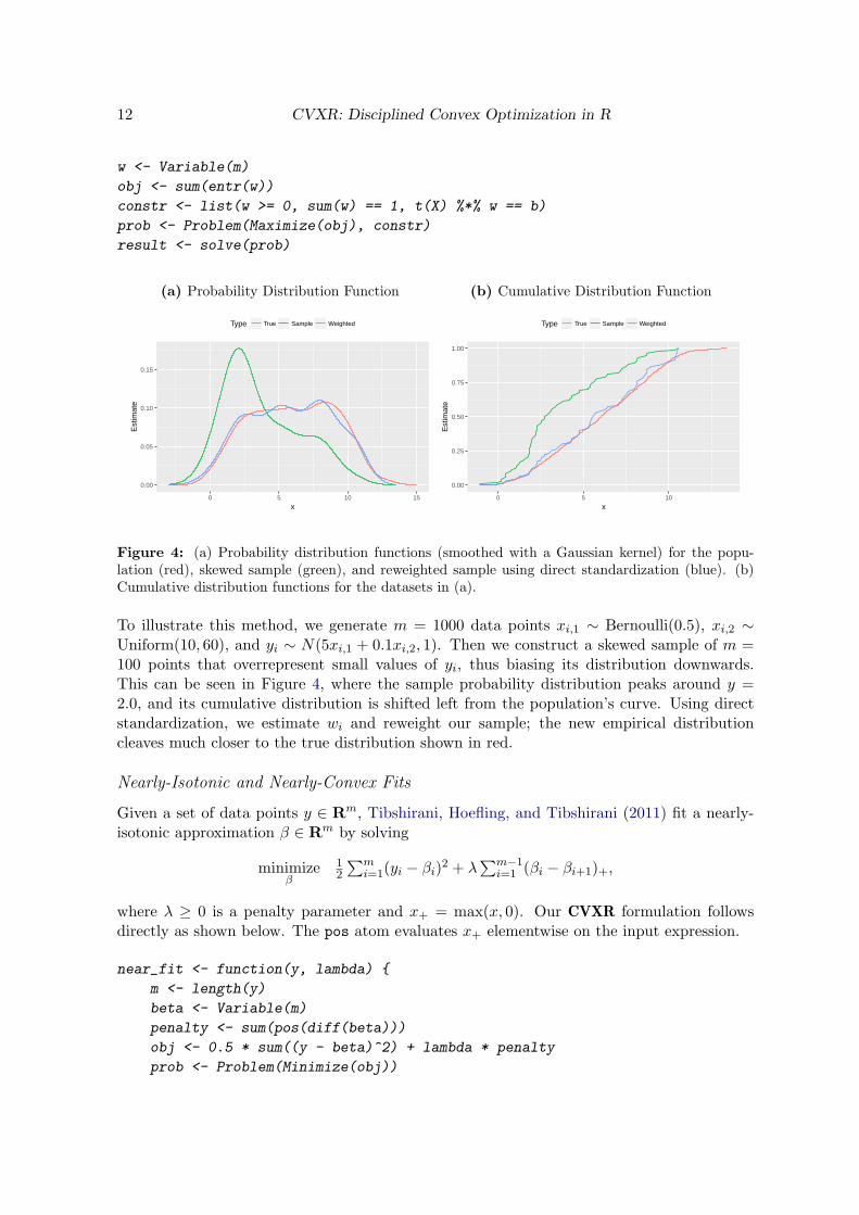
Figure 4: (a) Probability distribution functions (smoothed with a Gaussian kernel) for the popu-lation (red), skewed sample (green), and reweighted sample using direct standardization (blue). (b)Cumulative distribution functions for the datasets in (a).

To illustrate this method, we generate m = 1000 data points xi,1 ∼ Bernoulli(0.5), xi,2 ∼Uniform(10, 60), and yi ∼ N(5xi,1 + 0.1xi,2, 1). Then we construct a skewed sample of m =100 points that overrepresent small values of yi, thus biasing its distribution downwards.This can be seen in Figure 4, where the sample probability distribution peaks around y =2.0, and its cumulative distribution is shifted left from the population’s curve. Using directstandardization, we estimate wi and reweight our sample; the new empirical distributioncleaves much closer to the true distribution shown in red.

Nearly-Isotonic and Nearly-Convex Fits

Given a set of data points y ∈ Rm, Tibshirani, Hoefling, and Tibshirani (2011) fit a nearly-isotonic approximation β ∈ Rm by solving

minimizeβ

12

∑mi=1(yi − βi)

2 + λ∑m−1

i=1 (βi − βi+1)+,

where λ ≥ 0 is a penalty parameter and x+ = max(x, 0). Our CVXR formulation followsdirectly as shown below. The pos atom evaluates x+ elementwise on the input expression.

near_fit <- function(y, lambda) {

m <- length(y)

beta <- Variable(m)

penalty <- sum(pos(diff(beta)))

obj <- 0.5 * sum((y - beta)^2) + lambda * penalty




result$getValue(beta)

}

(a) Nearly-Isotonic

●

●●

●●●

●

●●

●

●

●

●

●

●

●●

●

●●●

●

●

●

●●●

●

●

●●●●

●

●●●

●

●

●

●

●

●●

●●

●●

●

●

●

●

●

●

●

●

●

●

●●●

●

●●

●

●

●

●

●

●●

●

●●●

●

●

●●

●

●

●

●

●

●

●●

●●

●

●●

●●

●

●

●●●

●

●

●

●

●

●

●

●

●

●●

●

●●●

●

●

●●

●

●

●

●

●

●

●

●

●

●

●

●●

●

●

●

●●

●

●●

●

●

●

●

●

●

●

●

●

●

●●

●

●●

●

●

●●

●

●

●

●

●●

●

●

−0.4

0.0

0.4

0.8

1850 1900 1950 2000

Year

Tem

pera

ture

Ano

mal

ies

(b) Nearly-Convex

●

●●

●●●

●

●●

●

●

●

●

●

●

●●

●

●●●

●

●

●

●●●

●

●

●●●●

●

●●●

●

●

●

●

●

●●

●●

●●

●

●

●

●

●

●

●

●

●

●

●●●

●

●●

●

●

●

●

●

●●

●

●●●

●

●

●●

●

●

●

●

●

●

●●

●●

●

●●

●●

●

●

●●●

●

●

●

●

●

●

●

●

●

●●

●

●●●

●

●

●●●

●

●

●

●

●

●

●

●

●

●

●●

●

●

●

●●

●

●●

●

●

●

●

●

●

●

●

●

●

●●

●

●●

●

●

●●

●

●

●

●

●●

●

●

−0.4

0.0

0.4

0.8

1850 1900 1950 2000

Year

Tem

pera

ture

Ano

mal

ies

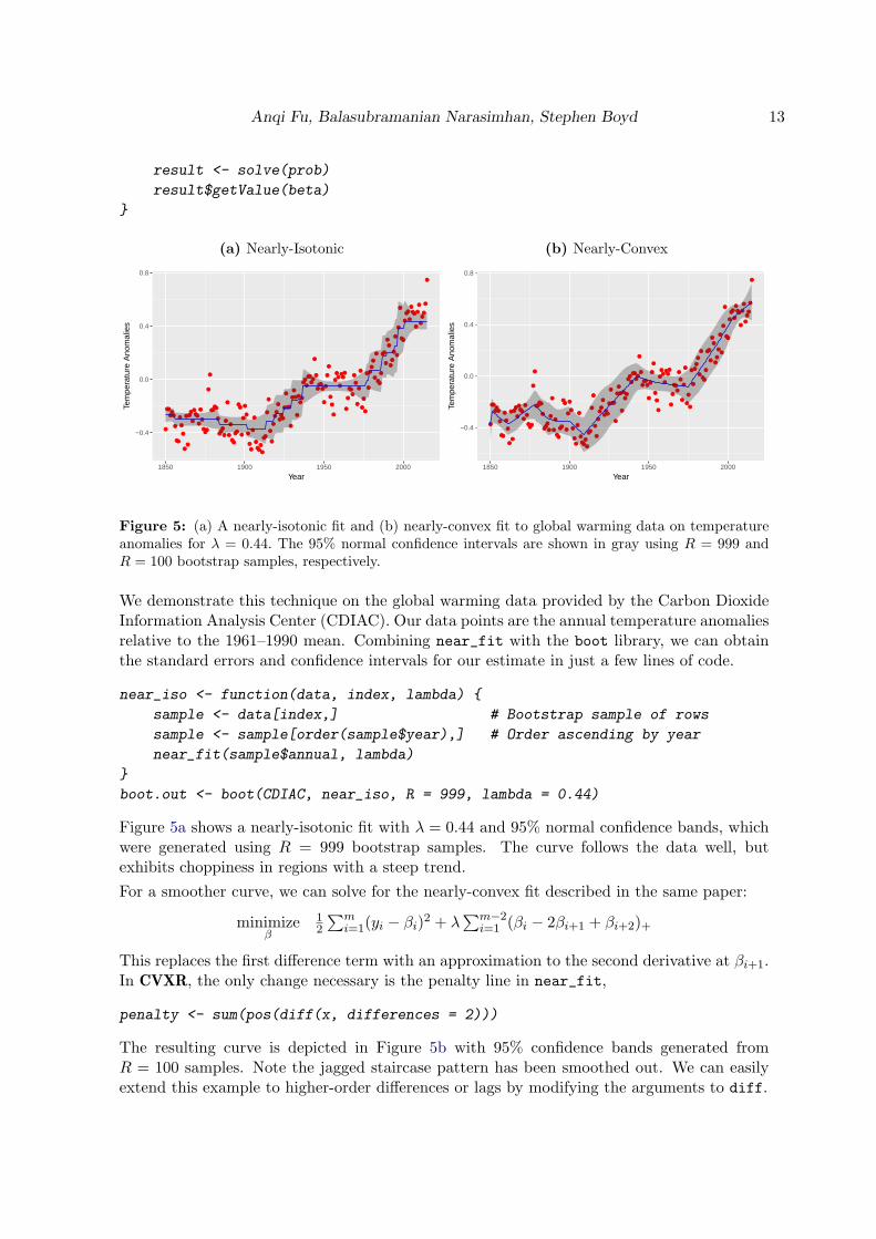
Figure 5: (a) A nearly-isotonic fit and (b) nearly-convex fit to global warming data on temperatureanomalies for λ = 0.44. The 95% normal confidence intervals are shown in gray using R = 999 andR = 100 bootstrap samples, respectively.

We demonstrate this technique on the global warming data provided by the Carbon DioxideInformation Analysis Center (CDIAC). Our data points are the annual temperature anomaliesrelative to the 1961–1990 mean. Combining near_fit with the boot library, we can obtainthe standard errors and confidence intervals for our estimate in just a few lines of code.

near_iso <- function(data, index, lambda) {

sample <- data[index,] # Bootstrap sample of rows

sample <- sample[order(sample$year),] # Order ascending by year

near_fit(sample$annual, lambda)

}

boot.out <- boot(CDIAC, near_iso, R = 999, lambda = 0.44)

Figure 5a shows a nearly-isotonic fit with λ = 0.44 and 95% normal confidence bands, whichwere generated using R = 999 bootstrap samples. The curve follows the data well, butexhibits choppiness in regions with a steep trend.

For a smoother curve, we can solve for the nearly-convex fit described in the same paper:

minimizeβ

12

∑mi=1(yi − βi)

2 + λ∑m−2

i=1 (βi − 2βi+1 + βi+2)+

This replaces the first difference term with an approximation to the second derivative at βi+1.In CVXR, the only change necessary is the penalty line in near_fit,

penalty <- sum(pos(diff(x, differences = 2)))

The resulting curve is depicted in Figure 5b with 95% confidence bands generated fromR = 100 samples. Note the jagged staircase pattern has been smoothed out. We can easilyextend this example to higher-order differences or lags by modifying the arguments to diff.


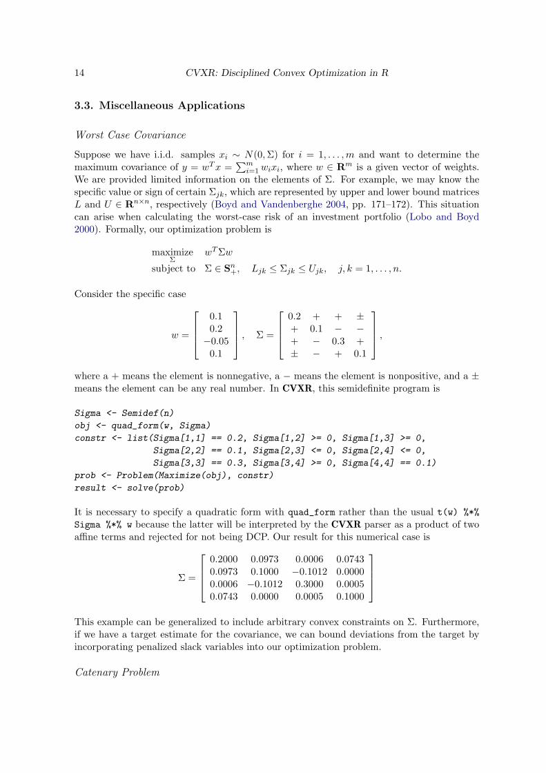
3.3. Miscellaneous Applications

Worst Case Covariance

Suppose we have i.i.d. samples xi ∼ N(0,Σ) for i = 1, . . . ,m and want to determine themaximum covariance of y = wTx =

∑mi=1wixi, where w ∈ Rm is a given vector of weights.

We are provided limited information on the elements of Σ. For example, we may know thespecific value or sign of certain Σjk, which are represented by upper and lower bound matricesL and U ∈ Rn×n, respectively (Boyd and Vandenberghe 2004, pp. 171–172). This situationcan arise when calculating the worst-case risk of an investment portfolio (Lobo and Boyd2000). Formally, our optimization problem is

maximizeΣ

wTΣw

subject to Σ ∈ Sn+, Ljk ≤ Σjk ≤ Ujk, j, k = 1, . . . , n.

Consider the specific case

w =

0.10.2

−0.050.1

, Σ =

0.2 + + ±+ 0.1 − −+ − 0.3 +± − + 0.1

,

where a + means the element is nonnegative, a − means the element is nonpositive, and a ±means the element can be any real number. In CVXR, this semidefinite program is

Sigma <- Semidef(n)

obj <- quad_form(w, Sigma)

constr <- list(Sigma[1,1] == 0.2, Sigma[1,2] >= 0, Sigma[1,3] >= 0,

Sigma[2,2] == 0.1, Sigma[2,3] <= 0, Sigma[2,4] <= 0,

Sigma[3,3] == 0.3, Sigma[3,4] >= 0, Sigma[4,4] == 0.1)



It is necessary to specify a quadratic form with quad_form rather than the usual t(w) %*%

Sigma %*% w because the latter will be interpreted by the CVXR parser as a product of twoaffine terms and rejected for not being DCP. Our result for this numerical case is

Σ =

0.2000 0.0973 0.0006 0.07430.0973 0.1000 −0.1012 0.00000.0006 −0.1012 0.3000 0.00050.0743 0.0000 0.0005 0.1000

This example can be generalized to include arbitrary convex constraints on Σ. Furthermore,if we have a target estimate for the covariance, we can bound deviations from the target byincorporating penalized slack variables into our optimization problem.

Catenary Problem


●

●

0.00

0.25

0.50

0.75

1.00

0.00 0.25 0.50 0.75 1.00

x

y

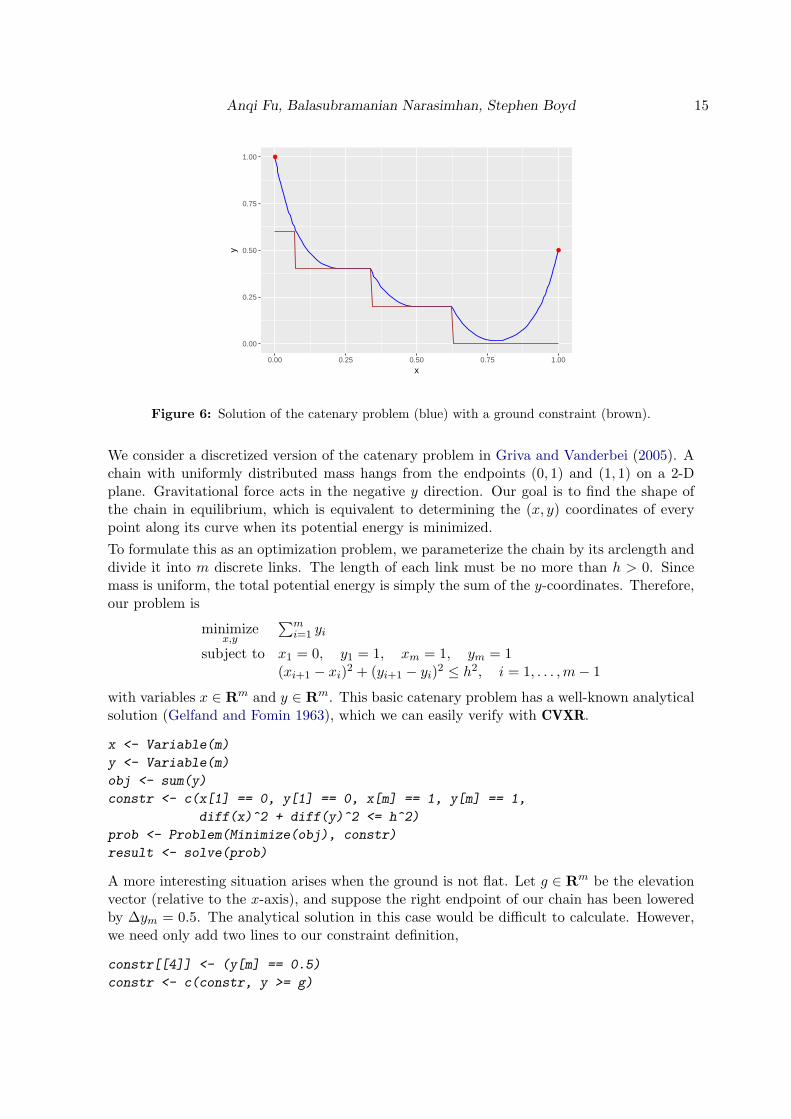
Figure 6: Solution of the catenary problem (blue) with a ground constraint (brown).

We consider a discretized version of the catenary problem in Griva and Vanderbei (2005). Achain with uniformly distributed mass hangs from the endpoints (0, 1) and (1, 1) on a 2-Dplane. Gravitational force acts in the negative y direction. Our goal is to find the shape ofthe chain in equilibrium, which is equivalent to determining the (x, y) coordinates of everypoint along its curve when its potential energy is minimized.

To formulate this as an optimization problem, we parameterize the chain by its arclength anddivide it into m discrete links. The length of each link must be no more than h > 0. Sincemass is uniform, the total potential energy is simply the sum of the y-coordinates. Therefore,our problem is

minimizex,y

∑mi=1 yi

subject to x1 = 0, y1 = 1, xm = 1, ym = 1(xi+1 − xi)

2 + (yi+1 − yi)2 ≤ h2, i = 1, . . . ,m− 1

with variables x ∈ Rm and y ∈ Rm. This basic catenary problem has a well-known analyticalsolution (Gelfand and Fomin 1963), which we can easily verify with CVXR.

x <- Variable(m)

y <- Variable(m)

obj <- sum(y)

constr <- c(x[1] == 0, y[1] == 0, x[m] == 1, y[m] == 1,

diff(x)^2 + diff(y)^2 <= h^2)



A more interesting situation arises when the ground is not flat. Let g ∈ Rm be the elevationvector (relative to the x-axis), and suppose the right endpoint of our chain has been loweredby ∆ym = 0.5. The analytical solution in this case would be difficult to calculate. However,we need only add two lines to our constraint definition,

constr[[4]] <- (y[m] == 0.5)

constr <- c(constr, y >= g)


to obtain the new result. Figure 6 depicts the solution of this modified catenary problemfor m = 101 and h = 0.04. The chain is shown hanging in blue, bounded below by the redstaircase structure, which represents the ground.

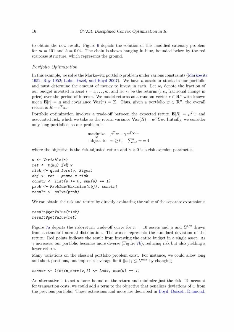
Portfolio Optimization

In this example, we solve the Markowitz portfolio problem under various constraints (Markowitz1952; Roy 1952; Lobo, Fazel, and Boyd 2007). We have n assets or stocks in our portfolioand must determine the amount of money to invest in each. Let wi denote the fraction ofour budget invested in asset i = 1, . . . ,m, and let ri be the returns (i.e., fractional change inprice) over the period of interest. We model returns as a random vector r ∈ Rn with knownmean E[r] = µ and covariance Var(r) = Σ. Thus, given a portfolio w ∈ Rn, the overallreturn is R = rTw.

Portfolio optimization involves a trade-off between the expected return E[R] = µTw andassociated risk, which we take as the return variance Var(R) = wTΣw. Initially, we consideronly long portfolios, so our problem is

maximizew

µTw − γwTΣw

subject to w ≥ 0,∑n

i=1w = 1

where the objective is the risk-adjusted return and γ > 0 is a risk aversion parameter.

w <- Variable(n)

ret <- t(mu) %*% w

risk <- quad_form(w, Sigma)

obj <- ret - gamma * risk

constr <- list(w >= 0, sum(w) == 1)



We can obtain the risk and return by directly evaluating the value of the separate expressions:

result$getValue(risk)

result$getValue(ret)

Figure 7a depicts the risk-return trade-off curve for n = 10 assets and µ and Σ1/2 drawnfrom a standard normal distribution. The x-axis represents the standard deviation of thereturn. Red points indicate the result from investing the entire budget in a single asset. Asγ increases, our portfolio becomes more diverse (Figure 7b), reducing risk but also yielding alower return.

Many variations on the classical portfolio problem exist. For instance, we could allow longand short positions, but impose a leverage limit ∥w∥1 ≤ Lmax by changing

constr <- list(p_norm(w,1) <= Lmax, sum(w) == 1)

An alternative is to set a lower bound on the return and minimize just the risk. To accountfor transaction costs, we could add a term to the objective that penalizes deviations of w fromthe previous portfolio. These extensions and more are described in Boyd, Busseti, Diamond,


(a) Risk-Return Curve

●

●

●

●

●

●

●

●

●

●

●

●

●

●

γ = 0.03γ = 0.09

γ = 0.29

γ = 0.93

0.0

0.5

1.0

1.5

1 2 3

Risk (Standard Deviation)

Ret

urn

(b) Asset Portfolios

0.00

0.25

0.50

0.75

1.00

γ = 0.03 γ = 0.09 γ = 0.29 γ = 0.93

Risk Aversion

Fra

ctio

n of

Bud

get

Figure 7: (a) Risk-return trade-off curve for various γ. Portfolios that invest completely in one assetare plotted in red. (b) Fraction of budget invested in each asset.

Kahn, Koh, Nystrup, and Speth (2017). The key takeaway is that all of these convex problemscan be easily solved in CVXR with just a few alterations to the code above.

Kelly Gambling

In Kelly gambling (Kelly 1956), we are given the opportunity to bet on n possible outcomes,which yield a random non-negative return of r ∈ Rn

+. The return r takes on exactly K valuesr1, . . . , rK with known probabilities π1, . . . , πK . This gamble is repeated over T periods. In agiven period t, let bi ≥ 0 denote the fraction of our wealth bet on outcome i. Assuming thenth outcome is equivalent to not wagering (it returns one with certainty), the fractions mustsatisfy

∑ni=1 bi = 1. Thus, at the end of the period, our cumulative wealth is wt = (rT b)wt−1.

Our goal is to maximize the average growth rate with respect to b ∈ Rn:

maximizeb

∑Kj=1 πj log(r

Tj b)

subject to b ≥ 0,∑n

i=1 bi = 1.

In the following code, rets is the K × n matrix of possible returns with row ri, while ps isthe vector of return probabilities (π1, . . . , πK).

b <- Variable(n)

obj <- t(ps) %*% log(rets %*% b)

constr <- list(b >= 0, sum(b) == 1)



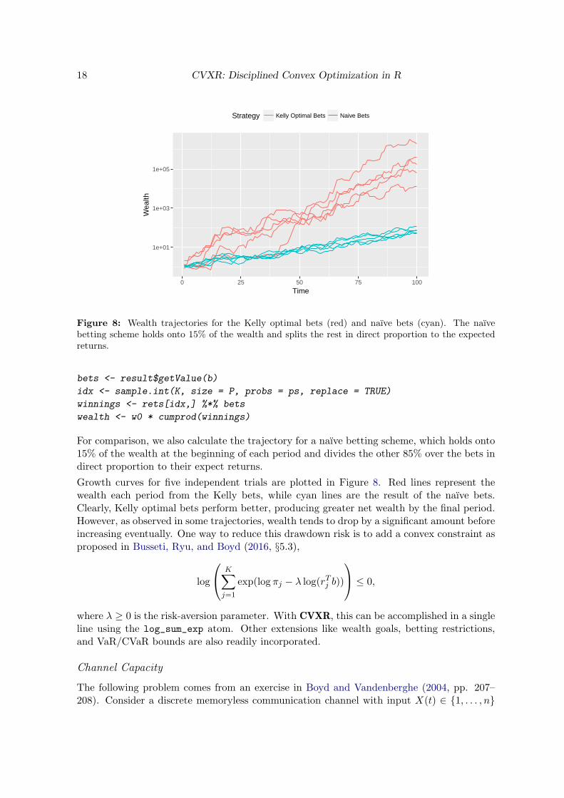
We solve the Kelly gambling problem for K = 100 and n = 20. The probabilities πj ∼Uniform(0, 1), and the potential returns rj ∼ Uniform(0.5, 1.5) except for rn = 1, whichrepresents the payoff from not wagering. With an initial wealth of w0 = 1, we simulate thegrowth trajectory of our Kelly optimal bets over P = 100 periods, assuming returns are i.i.d.over time.


1e+01

1e+03

1e+05

0 25 50 75 100

Time

Wea

lth

Strategy Kelly Optimal Bets Naive Bets

Figure 8: Wealth trajectories for the Kelly optimal bets (red) and naıve bets (cyan). The naıvebetting scheme holds onto 15% of the wealth and splits the rest in direct proportion to the expectedreturns.

bets <- result$getValue(b)

idx <- sample.int(K, size = P, probs = ps, replace = TRUE)

winnings <- rets[idx,] %*% bets

wealth <- w0 * cumprod(winnings)

For comparison, we also calculate the trajectory for a naıve betting scheme, which holds onto15% of the wealth at the beginning of each period and divides the other 85% over the bets indirect proportion to their expect returns.

Growth curves for five independent trials are plotted in Figure 8. Red lines represent thewealth each period from the Kelly bets, while cyan lines are the result of the naıve bets.Clearly, Kelly optimal bets perform better, producing greater net wealth by the final period.However, as observed in some trajectories, wealth tends to drop by a significant amount beforeincreasing eventually. One way to reduce this drawdown risk is to add a convex constraint asproposed in Busseti, Ryu, and Boyd (2016, §5.3),

log

K∑j=1

exp(log πj − λ log(rTj b))

≤ 0,

where λ ≥ 0 is the risk-aversion parameter. With CVXR, this can be accomplished in a singleline using the log_sum_exp atom. Other extensions like wealth goals, betting restrictions,and VaR/CVaR bounds are also readily incorporated.

Channel Capacity

The following problem comes from an exercise in Boyd and Vandenberghe (2004, pp. 207–208). Consider a discrete memoryless communication channel with input X(t) ∈ {1, . . . , n}


and output Y (t) ∈ {1, . . . ,m} for t = 1, 2, . . .. The relation between the input and output isgiven by a transition matrix P ∈ Rm×n

+ with

Pij = P(Y (t) = i|X(t) = j), i = 1, . . . ,m, j = 1, . . . , n

Assume that X has a probability distribution denoted by x ∈ Rn, i.e., xj = P(X(t) = j) forj = 1, . . . , n. A famous result by Shannon and Weaver (1949) states that the channel capacityis found by maximizing the mutual information between X and Y ,

I(X,Y ) =n∑

j=1

xj

m∑i=1

Pij log2 Pij −m∑i=1

yi log2 yi.

where y = Px is the probability distribution of Y . Since I is concave, this is equivalent tosolving the convex optimization problem

maximizex,y

∑nj=1 xj

∑mi=1 Pij logPij −

∑mi=1 yi log yi

subject to x ≥ 0,∑m

i=1 xi = 1, y = Px

for x ∈ Rn and y ∈ Rm. The associated code in CVXR is

x <- Variable(n)

y <- P %*% x

c <- apply(P * log2(P), 2, sum)

obj <- c %*% x + sum(entr(y))

constr <- list(sum(x) == 1, x >= 0)



The channel capacity is simply the optimal objective, result$value.

Fastest Mixing Markov Chain

This example is derived from the results in Boyd, Diaconis, and Xiao (2004, §2). LetG = (V, E) be a connected graph with vertices V = {1, . . . , n} and edges E ⊆ V × V. Assumethat (i, i) ∈ E for all i = 1, . . . , n, and (i, j) ∈ E implies (j, i) ∈ E . Under these conditions, adiscrete-time Markov chain on V will have the uniform distribution as one of its equilibriumdistributions. We are interested in finding the Markov chain, i.e.constructing the transitionprobability matrix P ∈ Rn×n

+ , that minimizes its asymptotic convergence rate to the uni-form distribution. This is an important problem in Markov chain Monte Carlo (MCMC)simulations, as it directly affects the sampling efficiency of an algorithm.

The asymptotic rate of convergence is determined by the second largest eigenvalue of P , whichin our case is µ(P ) := λmax(P − 1

n11T ) where λmax(A) denotes the maximum eigenvalue of

A. As µ(P ) decreases, the mixing rate increases and the Markov chain converges faster toequilibrium. Thus, our optimization problem is

minimizeP

λmax(P − 1n11

T )

subject to P ≥ 0, P1 = 1, P = P T

Pij = 0, (i, j) /∈ E .


(a) Triangle + 1 Edge

0.55

0.36

0.36

0.45

0.45

0.27

0.27

0.27

0.360.27

0.36

1

2

3

4

(b) Bipartite 2 + 3

0.14

0.43

0.14

0.43

0.43

0.29

0.29

0.29

0.29

0.29

0.29

0.29

0.29

0.29

0.29

0.29

0.29

1

2

3

4

5

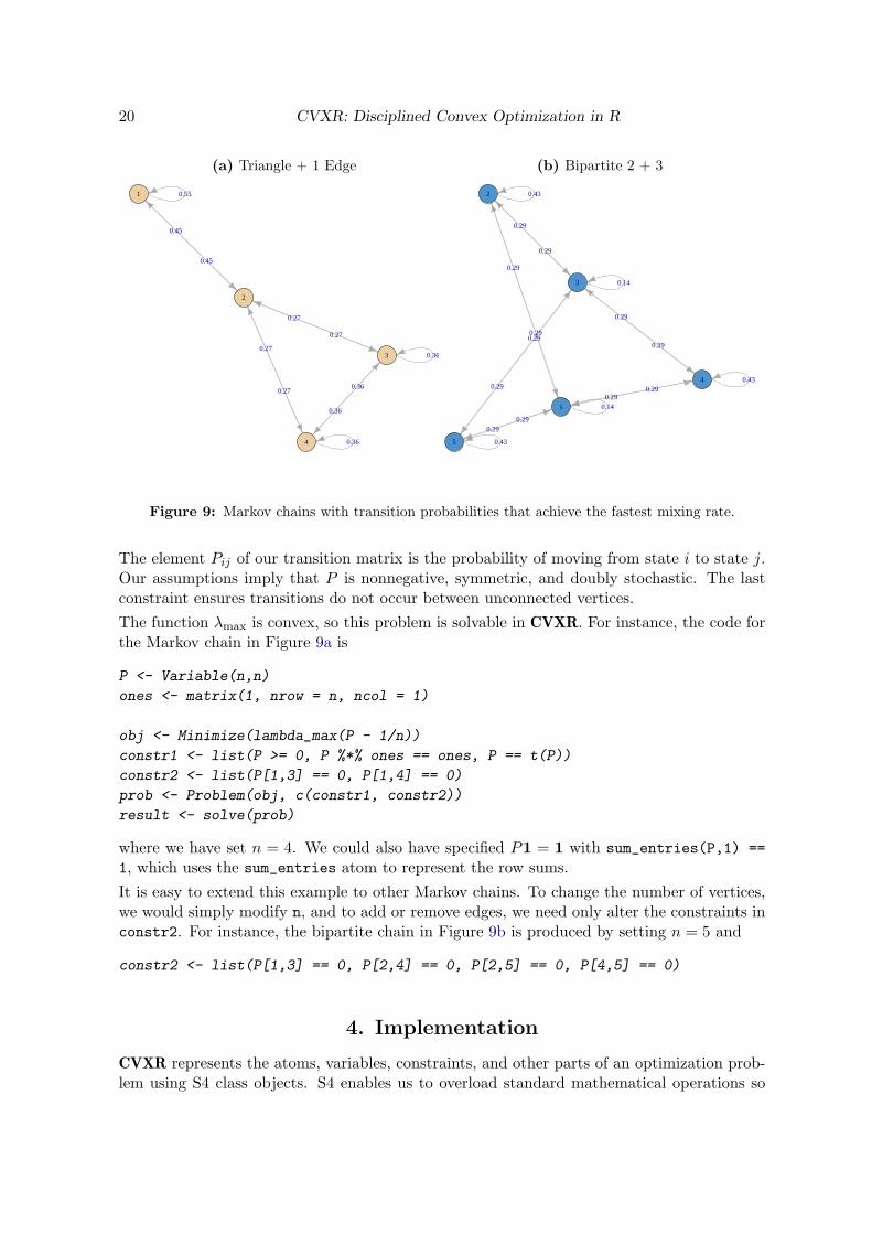
Figure 9: Markov chains with transition probabilities that achieve the fastest mixing rate.

The element Pij of our transition matrix is the probability of moving from state i to state j.Our assumptions imply that P is nonnegative, symmetric, and doubly stochastic. The lastconstraint ensures transitions do not occur between unconnected vertices.

The function λmax is convex, so this problem is solvable in CVXR. For instance, the code forthe Markov chain in Figure 9a is

P <- Variable(n,n)

ones <- matrix(1, nrow = n, ncol = 1)

obj <- Minimize(lambda_max(P - 1/n))

constr1 <- list(P >= 0, P %*% ones == ones, P == t(P))

constr2 <- list(P[1,3] == 0, P[1,4] == 0)

prob <- Problem(obj, c(constr1, constr2))


where we have set n = 4. We could also have specified P1 = 1 with sum_entries(P,1) ==

1, which uses the sum_entries atom to represent the row sums.

It is easy to extend this example to other Markov chains. To change the number of vertices,we would simply modify n, and to add or remove edges, we need only alter the constraints inconstr2. For instance, the bipartite chain in Figure 9b is produced by setting n = 5 and

constr2 <- list(P[1,3] == 0, P[2,4] == 0, P[2,5] == 0, P[4,5] == 0)

4. Implementation

CVXR represents the atoms, variables, constraints, and other parts of an optimization prob-lem using S4 class objects. S4 enables us to overload standard mathematical operations so


CVXR combines seamlessly with native R script and other packages. When an operation isinvoked on a variable, a new object is created that represents the corresponding expressiontree with the operator as the root node and the arguments as leaves. This tree grows auto-matically as more elements are added, allowing us to encapsulate the structure of an objectivefunction or constraint.

Once the user calls solve, DCP verification occurs. CVXR traverses the expression treerecursively, determining the sign and curvature of each sub-expression based on the propertiesof its component atoms. If the problem is deemed compliant, it is transformed into anequivalent cone program using graph implementations of convex functions (Grant et al. 2006).Then, CVXR passes the problem’s description to the CVXcanon C++ library, which generatesdata for the cone program, and sends this data to the solver-specific R interface. The solver’sresults are returned to the user in a list. This object-oriented design and infrastructure werelargely borrowed from CVXPY. Currently, the canonicalization and construction of data inR for the solver dominates computation time.

CVXR interfaces with the open-source cone solvers ECOS (Domahidi, Chu, and Boyd 2013)and SCS (O’Donoghue, Chu, Parikh, and Boyd 2016) through their respective R packages.ECOS is an interior-point solver, which achieves high accuracy for small and medium-sizedproblems, while SCS is a first-order solver that is capable of handling larger problems andsemidefinite constraints. Both solvers run single-threaded at present. Support for multi-threaded SCS will be added in the future, along with solvers like MOSEK (Andersen andAndersen 2000), GUROBI (Gurobi Optimization, Inc 2016), etc. It is not difficult to con-nect additional solvers so long as the solver has an API that can communicate with R.Users who wish to employ a custom solver may obtain the canonicalized data directly withget_problem_data.

We have provided a rich library of atoms, which should be sufficient to model most convexoptimization problems. However, it is possible for a sophisticated user to incorporate newatoms into this library. The process entails creating a S4 class for the atom, overloadingmethods that characterize its DCP properties, and representing its graph implementation as alist of linear operators that specify the corresponding feasibility problem. A full mathematicalexposition may be found in Grant et al. (2006, §10). Many problems can be reformulatedto comply with DCP by defining new variables and constraints as illustrated in Boyd andVandenberghe (2004). In general, we suggest users try this approach first before attemptingto add a novel atom.

5. Conclusion

Convex optimization plays an essential role in many fields, particularly machine learning andstatistics. CVXR provides an object-oriented language with which users can easily formulate,modify, and solve a broad range of convex optimization problems. While other R packagesmay perform faster on a subset of these problems, CVXR’s advantage is its flexibility andsimple intuitive syntax, making it an ideal tool for prototyping new models for which customR code does not exist. For more information, see the official CRAN site and documentation.

https://cran.r-project.org/package=CVXR


Acknowledgements

The authors would like to thank Trevor Hastie, Robert Tibshirani, John Chambers, DavidDonoho, and Hans Werner Borchers for their thoughtful advice and comments on this project.We are grateful to Steven Diamond, John Miller, and Paul Kunsberg Rosenfield for theircontributions to the software’s development. In particular, we are indebted to Steven for hiswork on CVXPY. Most of CVXR’s code, documentation, and examples were ported from hisPython library.

Anqi Fu’s research was supported by the Stanford Graduate Fellowship and DARPA X-DATAprogram. Balasubramanian Narasimhan’s work was supported by the Clinical and Transla-tional Science Award 1UL1 RR025744 for the Stanford Center for Clinical and TranslationalEducation and Research (Spectrum) from the National Center for Research Resources, Na-tional Institutes of Health.

References

Andersen ED, Andersen KD (2000). “The MOSEK Interior Point Optimizer for Linear Pro-gramming: An Implementation of the Homogeneous Algorithm.” In High PerformanceOptimization, pp. 197–232. Springer.

Andersen M, Dahl J, Liu Z, Vandenberghe L (2011). “Interior-Point Methods for Large-ScaleCone Programming.” Optimization for machine learning, 5583.

Boyd N, Hastie T, Boyd S, Recht B, Jordan M (2016). “Saturating Splines and FeatureSelection.” arXiv preprint arXiv:1609.06764.

Boyd S, Busseti E, Diamond S, Kahn RN, Koh K, Nystrup P, Speth J (2017). “Multi-PeriodTrading via Convex Optimization.” Foundations and Trends in Optimization.

Boyd S, Diaconis P, Xiao L (2004). “Fastest Mixing Markov Chain on a Graph.” SIAMReview, 46(4), 667–689.

Boyd S, Parikh N, Chu E, Peleato B, Eckstein J (2011). “Distributed Optimization andStatistical Learning via the Alternating Direction Method of Multipliers.” Foundations andTrends in Machine Learning, 3(1), 1–122.

Boyd S, Vandenberghe L (2004). Convex Optimization. Cambridge University Press.

Busseti E, Ryu EK, Boyd S (2016). “Risk–Constrained Kelly Gambling.” Journal of Investing,25(3), 118–134.

Cox DR (1958). “The Regression Analysis of Binary Sequences.” Journal of the Royal Statis-tical Society. Series B (Methodological), 20(2), 215–242.

Diamond S, Boyd S (2016). “CVXPY: A Python-Embedded Modeling Language for ConvexOptimization.” Journal of Machine Learning Research, 17(83), 1–5.

Domahidi A, Chu E, Boyd S (2013). “ECOS: An SOCP Solver for Embedded Systems.” InProceedings of the European Control Conference, pp. 3071–3076.


Dumbgen L, Rufibach K (2009). “Maximum Likelihood Estimation of a Log-Concave Densityand its Distribution Function: Basic Properties and Uniform Consistency.”Bernoulli, 15(1),40–68.

Fleiss JL, Levin B, Paik MC (2003). Statistical Methods for Rates and Proportions. Wiley-Interscience.

Freedman DA (2009). Statistical Models: Theory and Practice. Cambridge University Press.

Friedman J, Hastie T, Tibshirani R (2008). “Sparse Inverse Covariance Estimation with theGraphical Lasso.” Biostatistics, 9(3), 432–441.

Friedman J, Hastie T, Tibshirani R (2010). “Regularization Paths for Generalized LinearModels via Coordinate Descent.” Journal of Statistical Software, 33(1), 1–22.

Gelfand IM, Fomin SV (1963). Calculus of Variations. Prentice-Hall.

Grant M, Boyd S (2014). “CVX: MATLAB Software for Disciplined Convex Programming,Version 2.1.” http://cvxr.com/cvx.

Grant M, Boyd S, Ye Y (2006). “Disciplined Convex Programming.” In L Liberti, N Maculan(eds.), Global Optimization: From Theory to Implementation, Nonconvex Optimization andits Applications, pp. 155–210. Springer.

Griva IA, Vanderbei RJ (2005). “Case Studies in Optimization: Catenary problem.” Opti-mization and Engineering, 6(4), 463–482.

Gurobi Optimization, Inc (2016). Gurobi Optimizer Reference Manual. http://www.gurobi.com.

H Zou TH (2005). “Regularization and Variable Selection via the Elastic–Net.” Journal ofthe Royal Statistical Society. Series B (Methodological), 67(2), 301–320.

Hastie T, Tibshirani R, Friedman J (2001). The Elements of Statistical Learning. Springer.

Hornik K, Meyer D, Schwendinger F, Theussl S (2017). ROI: R Optimization Infrastructure.https://CRAN.R-project.org/package=ROI.

Huber PJ (1964). “Robust Estimation of a Location Parameter.” Annals of MathematicalStatistics, 35(1), 73–101.

Johnson SG (2008). The NLopt Nonlinear-Optimization Package. http://ab-initio.mit.edu/nlopt/.

Kelly JL (1956). “A New Interpretation of Information Rate.” Bell System Technical Journal,35(4), 917–926.

Koenker R (2005). Quantile Regression. Cambridge University Press.

Lobo M, Boyd S (2000). “The Worst-Case Risk of a Portfolio.” http://stanford.edu/

~boyd/papers/pdf/risk_bnd.pdf.

Lobo MS, Fazel M, Boyd S (2007). “Portfolio Optimization with Linear and Fixed TransactionCosts.” Annals of Operations Research, 152(1), 341–365.

http://cvxr.com/cvx

http://www.gurobi.com

http://www.gurobi.com

https://CRAN.R-project.org/package=ROI

http://stanford.edu/~boyd/papers/pdf/risk_bnd.pdf

http://stanford.edu/~boyd/papers/pdf/risk_bnd.pdf


Lofberg J (2004). “YALMIP: A Toolbox for Modeling and Optimization in MATLAB.” InProceedings of the IEEE International Symposium on Computed Aided Control SystemsDesign, pp. 294–289. http://users.isy.liu.se/johanl/yalmip.

Markowitz HM (1952). “Portfolio Selection.” Journal of Finance, 7(1), 77–91.

Nash JC, Varadhan R (2011). “Unifying Optimization Algorithms to Aid Software SystemUsers: optimx for R.” Journal of Statistical Software, 43(9), 1–14.

O’Donoghue B, Chu E, Parikh N, Boyd S (2016). “Conic Optimization via Operator Splittingand Homogeneous Self-Dual Embedding.” Journal of Optimization Theory and Applica-tions, pp. 1–27.

Roy AD (1952). “Safety First and the Holding of Assets.” Econometrica, 20(3), 431–449.

Shannon CE, Weaver W (1949). The Mathematical Theory of Communication. University ofIllinois Press.

Skajaa A, Ye Y (2015). “A Homogeneous Interior-Point Algorithm for Nonsymmetric ConvexConic Optimization.” Mathematical Programming, 150(2), 391–422.

Tibshirani RJ, Hoefling H, Tibshirani R (2011). “Nearly-Isotonic Regression.” Technometrics,53(1), 54–61.

Udell M, Mohan K, Zeng D, Hong J, Diamond S, Boyd S (2014). “Convex Optimizationin Julia.” In Proceedings of the Workshop for High Performance Technical Computing inDynamic Languages, pp. 18–28.

Wright SJ (1997). Primal-Dual Interior-Point Methods. SIAM.

http://users.isy.liu.se/johanl/yalmip


Affiliation:

Anqi FuDepartment of Electrical EngineeringDavid Packard Building350 Serra MallStanford, CA 94305E-mail: [email protected]: https://web.stanford.edu/~anqif/

Balasubramanian NarasimhanDepartment of Biomedical Data Sciences, andDepartment of StatisticsStanford University390 Serra MallStanford, CA 94305E-mail: [email protected]: https://statistics.stanford.edu/~naras/

Stephen BoydDepartment of Electrical EngineeringDavid Packard Building350 Serra MallStanford, CA 94305E-mail: [email protected]: https://web.stanford.edu/~boyd/

mailto:[email protected]

https://web.stanford.edu/~anqif/


https://statistics.stanford.edu/~naras/


https://web.stanford.edu/~boyd/

Documents

CVXR: An R Package for Disciplined Convex Optimization · CVXR: An R Package for Disciplined Convex Optimization Anqi Fu, Balasubramanian Narasimhan, and Stephen Boyd Abstract CVXR