Embed Size (px)
Citation preview
GROUND STATES FOR FRACTIONAL MAGNETIC OPERATORS
PIETRO D’AVENIA AND MARCO SQUASSINA
Abstract. We study a class of minimization problems for a nonlocal operator involving anexternal magnetic potential. The notions are physically justified and consistent with the case ofabsence of magnetic fields. Existence of solutions is obtained via concentration compactness.
Contents
1. Introduction and results 12. Functional setting 43. Preliminary stuff 84. Existence of minimizers 154.1. Subcritical symmetric case 154.2. Subcritical case 164.3. Critical case 19References 21
1. Introduction and results
Since the late nineties, nonlocal integral operators like
(1.1) (−∆)su(x) = cs limε0
∫Bcε(x)
u(x)− u(y)
|x− y|3+2sdy = F−1(|ξ|2sF(u)(ξ))(x), u ∈ C∞c (R3),
where s ∈ (0, 1) and
cs = s22s Γ(
3+2s2
)π3/2Γ(1− s)
,
being Γ the Gamma function, have been widely used in the theory of Levy processes. Indeed, inview of the Levy-Khintchine formula, the generator H of the semigroup on C∞c (R3) associatedto a general Levy process is given by
(1.2) H u(x) = −aij∂2xixju(x)−bi∂xiu(x)− lim
ε0
∫Bcε(0)
(u(x+y)−u(x)−1|y|<1(y)y ·∇u(x)
)dµ,
with summation on repeated indexes and where µ is a Levy nonnegative measure, namely∫R3
|y|2
1 + |y|2dµ <∞.
The last contribution in (1.2) represents the purely jump part of the Levy process, while thefirst two terms represent a Brownian motion with drift. It is now well established that Levyprocesses with jumps are more appropriate for some mathematical models in finance. AmongLevy processes, the only stochastically stable ones having jump part are those corresponding toradial measures as
dµ =cs
|y|3+2sdy,
2010 Mathematics Subject Classification. 49A50, 26A33, 74G65, 82D99.Key words and phrases. Fractional magnetic operators, minimization problems, concentration compactness.
1

2 P. D’AVENIA AND M. SQUASSINA
hence the importance of the definition (1.1). Moreover, the fractional Laplacian (1.1) allows todevelop a generalization of quantum mechanics and also to describe the motion of a chain or arrayof particles that are connected by elastic springs and unusual diffusion processes in turbulent fluidmotions and material transports in fractured media (for more details see e.g. [1,9,22,26] and thereferences therein). Due to the results of Bourgain-Brezis-Mironescu [5, 6], up to correcting theoperator (1.1) with the factor (1−s) it follows that (−∆)su converges to −∆u in the limit s 1.Thus, up to normalization, we may think the nonlocal case as an approximation of the local case.A pseudorelativistic extension of the Laplacian is the well known pseudodifferential operator√−∆ +m2 −m where m is a nonnegative number. This operator appears in the study of free
relativistic particles of mass m and√−∆ +m2 is defined by F−1(
√|ξ|2 +m2F(u)(ξ)) (see [23]
for more details). We observe that for m = 0 we have the operator in (1.1) with s = 1/2.An important role in the study of particles which interact, e.g. using the Weyl covariant derivative,with a magnetic field B = ∇×A, A : R3 → R3, is assumed by another extension of the Laplacian,namely the magnetic Laplacian (∇− iA)2 (see [3,27]). Nonlinear magnetic Schrodinger equationslike
−(∇− iA)2u+ u = f(u)
have been extensively studied (see e.g. [2, 8, 12,15,21,28]).In [19], Ichinose and Tamura, through oscillatory integrals, introduce the so-called Weyl pseudo-differential operator defined with mid-point prescription
HAu(x) =1
(2π)3
∫R6
ei(x−y)·ξ√∣∣∣ξ −A(x+ y
2
)∣∣∣2 +m2u(y)dydξ
=1
(2π)3
∫R6
ei(x−y)·
(ξ+A(x+y
2
))√|ξ|2 +m2u(y)dydξ
as a fractional relativistic generalization of the magnetic Laplacian (see also [17], the review
article [18] and the references therein). The operator HA takes the place of√−∆ +m2 and it is
possible to show that for all u ∈ C∞c (R3,C),
HAu(x) = mu(x)− limε0
∫Bcε(0)
[e−iy·A
(x+ y
2
)u(x+ y)− u(x)− 1|y|<1(y)y · (∇− iA(x))u(x)
]dµ
= mu(x) + limε0
∫Bcε(x)
[u(x)− ei(x−y)·A(x+y
2 )u(y)]µ(y − x)dy,
where
dµ = µ(y)dy =
2(m2π
)2 K2(m|y|)|y|2 dy, m > 0,
1π2|y|4dy, m = 0,
and K2 is the modified Bessel function of the third kind of order 2 (see e.g. [18, Subsection 3.1]).In this paper we are concerned with the operator
(1.3) (−∆)sAu(x) = cs limε0
∫Bcε(x)
u(x)− ei(x−y)·A(x+y2 )u(y)
|x− y|3+2sdy, x ∈ R3,
and, in particular, with ground state solutions of the equation
(Ps,A) (−∆)sAu+ u = |u|p−2u in R3.
The operator (1.3) is consistent with the definition of fractional Laplacian given in (1.1) if A = 0and with HA for m = 0 and s = 1/2. To our knowledge, this is the first mathematical contributionto the study of nonlinear problems involving operator (1.3).
For the sake of completeness we mention that there exist other different definitions of themagnetic pseudorelativistic operator (see [18, 20, 23]) and in [16] a fractional magnetic operator

GROUND STATES FOR FRACTIONAL MAGNETIC OPERATORS 3
(∇− iA)2s is defined through the spectral theorem (see also discussion on the different definitionsin [18, Proposition 2.6]).
Throughout the paper we consider magnetic potentials A’s which have locally bounded gradient.We now state our results.Let 2 < p < 6/(3− 2s) and consider the minimization problem
(MA) MA = infu∈S
(∫R3
|u|2dx+cs2
∫R6
|e−i(x−y)·A(x+y2 )u(x)− u(y)|2
|x− y|3+2sdxdy
),
where
S =u ∈ Hs
A(R3,C) :
∫R3
|u|pdx = 1
and HsA(R3,C) is a suitable Hilbert space defined in Section 2. Once a solution to MA exists,
due to the Lagrange Multiplier Theorem, we get a weak solution to (Ps,A), see Sections 2 and 4.When S is restricted to radially symmetric functions, the problem is denoted by MA,r.
First we give the following
Definition 1.1. We say that A satisfies assumption A , if for any unbounded sequence Ξ =ξnn∈N ⊂ R3 there exist a sequence Hnn∈N ⊂ R3 and a function AΞ : R3 → R3 such that
(1.4) limnAn(x) = AΞ(x) for all x ∈ R3 and sup
n‖An‖L∞(K) <∞ for all compact sets K,
where An(x) := A(x+ ξn) +Hn and ξn is a subsequence of Ξ such that |ξn| → ∞.
We also set X := Ξ = ξnn∈N unbounded : condition (1.4) holds. Observe that, if A admitslimit as |x| → ∞, then it satisfies assumption A .Our main result is
Theorem 1.2 (Subcritical case). The following facts hold:
(i) MA,r has a solution;(ii) if A is linear, then MA has a solution;
(iii) if A satisfies A and MA < infΞ∈X MAΞ, then MA has a solution.
We also consider the minimization problem
(M cA) M c
A := infu∈S c
cs2
∫R6
|e−i(x−y)·A(x+y2 )u(x)− u(y)|2
|x− y|3+2sdxdy,
where
S c =u ∈ Ds
A(R3,C) :
∫R3
|u|6/(3−2s)dx = 1
and DsA(R3,C) is a suitable Hilbert space defined in Subection 4.3. We are able to prove
Theorem 1.3 (Critical case). The following facts hold:
(i) if M cA has a solution u, there exist z ∈ R3, ε > 0 and ϑA : R3 → R such that
u(x) = ds
(ε
ε2 + |x− z|2
) 3−2s2
eiϑA(x);
(ii) if for some k ∈ N and E ⊂ R6 of positive measure
(x− y) ·A(x+ y
2
)6≡ 2kπ for all (x, y) ∈ E,
then M cA has no solution u of the form eiϑv(x) where ϑ ∈ R and v of fixed sign.

4 P. D’AVENIA AND M. SQUASSINA
The local version of the above results can be found in the work [15] by Esteban and Lions. In [14],for the case without magnetic field and with subcritical nonlinearities, existence of ground stateswas obtained using different arguments, namely without involving concentration compactnessarguments, but instead symmetrizing the minimizing sequences, by using∫
R6
||u(x)|∗ − |u(y)|∗|2
|x− y|3+2sdxdy ≤
∫R6
|u(x)− u(y)|2
|x− y|3+2sdxdy,
for all u ∈ Hs(R3), where v∗ denotes the Schwarz symmetrization of v : R3 → R+. On thecontrary, when A 6≡ 0, the inequality∫
R6
|e−i(x−y)·A(x+y2 )|u(x)|∗ − |u(y)|∗|2
|x− y|3+2sdxdy ≤
∫R6
|e−i(x−y)·A(x+y2 )u(x)− u(y)|2
|x− y|3+2sdxdy,
does not seem to work and a different strategy for the proof has to be outlined. Dealing with thenonlocal case, it is natural to expect that, in the study of minimizing sequences, the hardest stageis that of ruling out the dichotomy in the concentration compactness alternative. This is in factthe case, but thanks to a careful analysis developed in Lemma 3.9, dichotomy can be ruled outallowing for tightness and hence the strong convergence of minimizing sequences up translationsand phase changes.
We organize the paper in the following way: in Section 2 we introduce the functional setting ofthe problem and we provide some basic properties about it; in Section 3 we show further technicalfacts on the functional setting as well as some preliminary results about the Concentration-Compactness procedure; finally, in Section 4, we complete with the proofs of our results.
Acknowledgments. The research was partially supported by Gruppo Nazionale per l’AnalisiMatematica, la Probabilita e le loro Applicazioni (INdAM).
Notations. We denote by BR(ξ) a ball in R3 of center ξ and radius R. For a measurable setE ⊂ R3 we denote by Ec the complement of E in R3, namely Ec = R3 \ E. We denote by 1Ethe indicator function of E. The symbol Ln(Ω) stands for the Lebesgue measure of a measurablesubset Ω ⊂ Rn. For a complex number z ∈ C, the symbol <z indicates its real part and =z itsimaginary part. The modulus of z is denoted by |z|. The standard norm of Lp spaces is denotedby ‖ · ‖Lp .
2. Functional setting
Let L2(R3,C) be the Lebesgue space of complex valued functions with summable square endowedwith the real scalar product
〈u, v〉L2 := <∫R3
uvdx, for all u, v ∈ L2(R3,C),
and A : R3 → R3 be a continuous function. We consider the magnetic Gagliardo semi-normdefined by
[u]2s,A :=cs2
∫R6
|e−i(x−y)·A(x+y2 )u(x)− u(y)|2
|x− y|3+2sdxdy,
the scalar product defined by
〈u, v〉s,A := 〈u, v〉L2 +cs2<∫R6
(e−i(x−y)·A(x+y
2 )u(x)− u(y))(
e−i(x−y)·A(x+y2 )v(x)− v(y)
)|x− y|3+2s
dxdy,
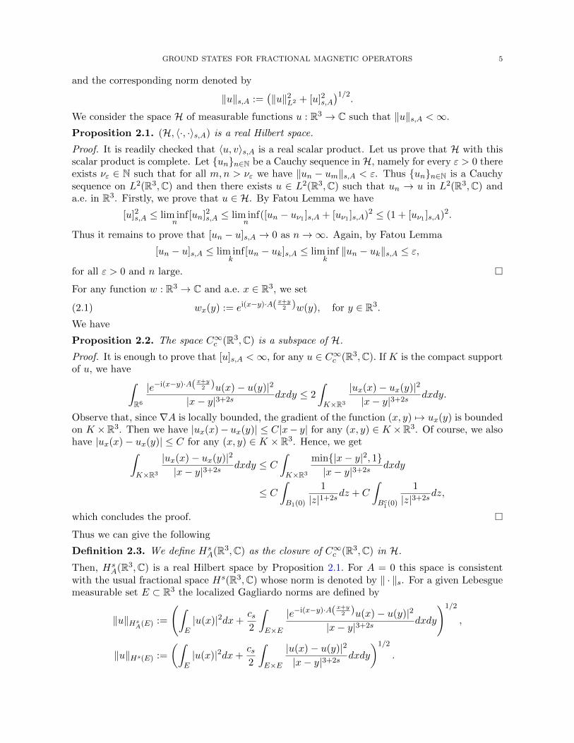
GROUND STATES FOR FRACTIONAL MAGNETIC OPERATORS 5
and the corresponding norm denoted by
‖u‖s,A :=(‖u‖2L2 + [u]2s,A
)1/2.
We consider the space H of measurable functions u : R3 → C such that ‖u‖s,A <∞.Proposition 2.1. (H, 〈·, ·〉s,A) is a real Hilbert space.
Proof. It is readily checked that 〈u, v〉s,A is a real scalar product. Let us prove that H with thisscalar product is complete. Let unn∈N be a Cauchy sequence in H, namely for every ε > 0 thereexists νε ∈ N such that for all m,n > νε we have ‖un − um‖s,A < ε. Thus unn∈N is a Cauchysequence on L2(R3,C) and then there exists u ∈ L2(R3,C) such that un → u in L2(R3,C) anda.e. in R3. Firstly, we prove that u ∈ H. By Fatou Lemma we have
[u]2s,A ≤ lim infn
[un]2s,A ≤ lim infn
([un − uν1 ]s,A + [uν1 ]s,A)2 ≤ (1 + [uν1 ]s,A)2.
Thus it remains to prove that [un − u]s,A → 0 as n→∞. Again, by Fatou Lemma
[un − u]s,A ≤ lim infk
[un − uk]s,A ≤ lim infk‖un − uk‖s,A ≤ ε,
for all ε > 0 and n large.
For any function w : R3 → C and a.e. x ∈ R3, we set
(2.1) wx(y) := ei(x−y)·A(x+y2 )w(y), for y ∈ R3.
We have
Proposition 2.2. The space C∞c (R3,C) is a subspace of H.
Proof. It is enough to prove that [u]s,A <∞, for any u ∈ C∞c (R3,C). If K is the compact supportof u, we have∫
R6
|e−i(x−y)·A(x+y2 )u(x)− u(y)|2
|x− y|3+2sdxdy ≤ 2
∫K×R3
|ux(x)− ux(y)|2
|x− y|3+2sdxdy.
Observe that, since ∇A is locally bounded, the gradient of the function (x, y) 7→ ux(y) is boundedon K ×R3. Then we have |ux(x)− ux(y)| ≤ C|x− y| for any (x, y) ∈ K ×R3. Of course, we alsohave |ux(x)− ux(y)| ≤ C for any (x, y) ∈ K × R3. Hence, we get∫
K×R3
|ux(x)− ux(y)|2
|x− y|3+2sdxdy ≤ C
∫K×R3
min|x− y|2, 1|x− y|3+2s
dxdy
≤ C∫B1(0)
1
|z|1+2sdz + C
∫Bc1(0)
1
|z|3+2sdz,
which concludes the proof.
Thus we can give the following
Definition 2.3. We define HsA(R3,C) as the closure of C∞c (R3,C) in H.
Then, HsA(R3,C) is a real Hilbert space by Proposition 2.1. For A = 0 this space is consistent
with the usual fractional space Hs(R3,C) whose norm is denoted by ‖ · ‖s. For a given Lebesguemeasurable set E ⊂ R3 the localized Gagliardo norms are defined by
‖u‖HsA(E) :=
(∫E|u(x)|2dx+
cs2
∫E×E
|e−i(x−y)·A(x+y2 )u(x)− u(y)|2
|x− y|3+2sdxdy
)1/2
,
‖u‖Hs(E) :=
(∫E|u(x)|2dx+
cs2
∫E×E
|u(x)− u(y)|2
|x− y|3+2sdxdy
)1/2
.
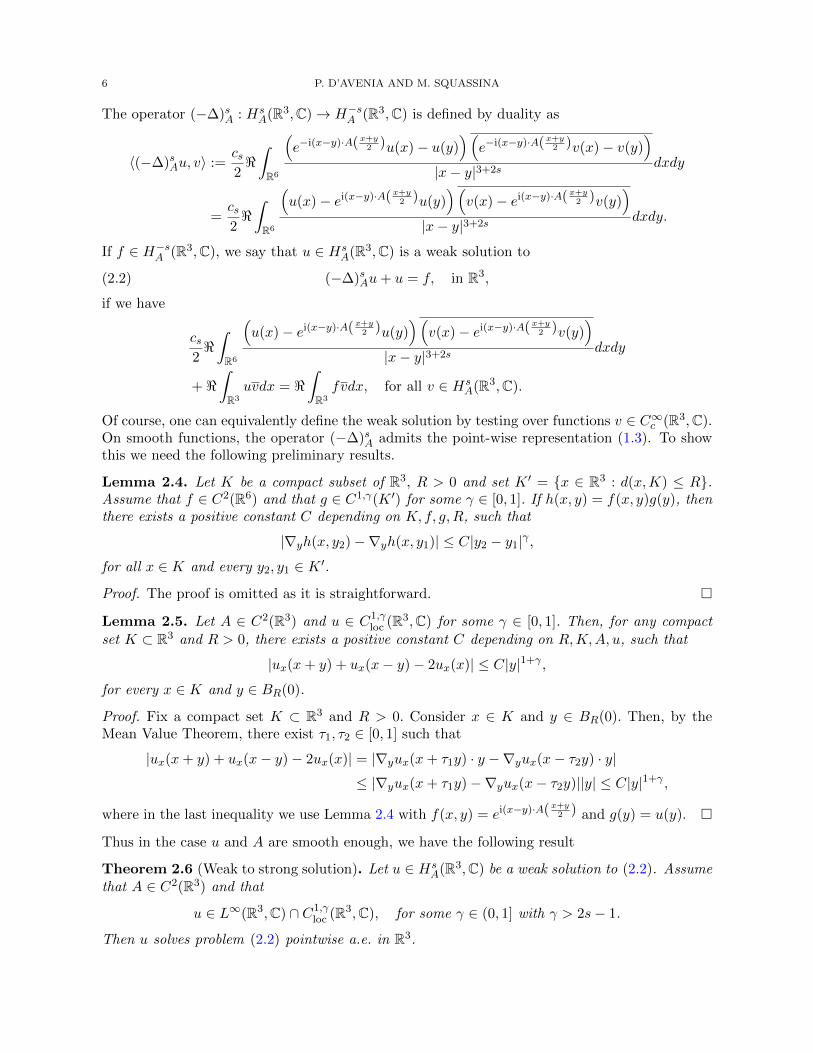
6 P. D’AVENIA AND M. SQUASSINA
The operator (−∆)sA : HsA(R3,C)→ H−sA (R3,C) is defined by duality as
〈(−∆)sAu, v〉 :=cs2<∫R6
(e−i(x−y)·A(x+y
2 )u(x)− u(y))(
e−i(x−y)·A(x+y2 )v(x)− v(y)
)|x− y|3+2s
dxdy
=cs2<∫R6
(u(x)− ei(x−y)·A(x+y
2 )u(y))(
v(x)− ei(x−y)·A(x+y2 )v(y)
)|x− y|3+2s
dxdy.
If f ∈ H−sA (R3,C), we say that u ∈ HsA(R3,C) is a weak solution to
(2.2) (−∆)sAu+ u = f, in R3,
if we have
cs2<∫R6
(u(x)− ei(x−y)·A(x+y
2 )u(y))(
v(x)− ei(x−y)·A(x+y2 )v(y)
)|x− y|3+2s
dxdy
+ <∫R3
uvdx = <∫R3
fvdx, for all v ∈ HsA(R3,C).
Of course, one can equivalently define the weak solution by testing over functions v ∈ C∞c (R3,C).On smooth functions, the operator (−∆)sA admits the point-wise representation (1.3). To showthis we need the following preliminary results.
Lemma 2.4. Let K be a compact subset of R3, R > 0 and set K ′ = x ∈ R3 : d(x,K) ≤ R.Assume that f ∈ C2(R6) and that g ∈ C1,γ(K ′) for some γ ∈ [0, 1]. If h(x, y) = f(x, y)g(y), thenthere exists a positive constant C depending on K, f, g,R, such that
|∇yh(x, y2)−∇yh(x, y1)| ≤ C|y2 − y1|γ ,
for all x ∈ K and every y2, y1 ∈ K ′.
Proof. The proof is omitted as it is straightforward.
Lemma 2.5. Let A ∈ C2(R3) and u ∈ C1,γloc (R3,C) for some γ ∈ [0, 1]. Then, for any compact
set K ⊂ R3 and R > 0, there exists a positive constant C depending on R,K,A, u, such that
|ux(x+ y) + ux(x− y)− 2ux(x)| ≤ C|y|1+γ ,
for every x ∈ K and y ∈ BR(0).
Proof. Fix a compact set K ⊂ R3 and R > 0. Consider x ∈ K and y ∈ BR(0). Then, by theMean Value Theorem, there exist τ1, τ2 ∈ [0, 1] such that
|ux(x+ y) + ux(x− y)− 2ux(x)| = |∇yux(x+ τ1y) · y −∇yux(x− τ2y) · y|≤ |∇yux(x+ τ1y)−∇yux(x− τ2y)||y| ≤ C|y|1+γ ,
where in the last inequality we use Lemma 2.4 with f(x, y) = ei(x−y)·A(x+y2 ) and g(y) = u(y).
Thus in the case u and A are smooth enough, we have the following result
Theorem 2.6 (Weak to strong solution). Let u ∈ HsA(R3,C) be a weak solution to (2.2). Assume
that A ∈ C2(R3) and that
u ∈ L∞(R3,C) ∩ C1,γloc (R3,C), for some γ ∈ (0, 1] with γ > 2s− 1.
Then u solves problem (2.2) pointwise a.e. in R3.

GROUND STATES FOR FRACTIONAL MAGNETIC OPERATORS 7
Proof. With the notation introduced in (2.1), the definition of weak solution writes as
(2.3)cs2<∫R6
(ux(x)− ux(y)) (vx(x)− vx(y))
|x− y|3+2sdxdy + <
∫R3
uvdx = <∫R3
fvdx,
for all v ∈ C∞c (R3,C). Let us fix a v ∈ C∞c (R3,C) and set K := supp(v). Now, for any ε > 0, weintroduce the auxiliary function gε : K → R defined by
gε(x) :=cs2
∫R3
ux(x)− ux(y)
|x− y|3+2s1Bcε(x)(y)dy.
Note that for all x ∈ K we have that
(2.4) gε(x)→ 1
2(−∆)sAu(x), as ε→ 0 whenever the limit exists.
Simple changes of variables show that gε can be equivalently written as
gε(x) = −cs4
∫R3
ux(x+ y) + ux(x− y)− 2ux(x)
|y|3+2s1Bcε(0)(y)dy.
Furthermore, by Lemma 2.5, there exist C > 0 and R > 0 such that
|ux(x+ y) + ux(x− y)− 2ux(x)| ≤ C|y|1+γ , for x ∈ K and y ∈ BR(0).
Therefore, taking into account that |ux(y)| ≤ ‖u‖L∞ for all y ∈ R3, we have the inequality
|ux(x+ y) + ux(x− y)− 2ux(x)||y|3+2s
≤ C
|y|2+2s−γ 1BR(0)(y) +C
|y|3+2s1BcR(0)(y),
for some constant C. Due to the assumption γ > 2s− 1, the right hand side belongs to L1(R3).Then, by dominated convergence, the limit of gε(x) as ε→ 0 exists a.e. in K and it is thus equalto 1
2(−∆)sAu(x) by (2.4). Since also |gε(x)| ≤ C a.e. in K, again the dominated convergenceyields
(2.5) gε →1
2(−∆)sAu, strongly in L1(K).
Now, the first term in formula (2.3) can be treated as follows
cs2
∫R6
(ux(x)− ux(y)) (vx(x)− vx(y))
|x− y|3+2sdxdy
= limε→0
cs2
∫R6
(ux(x)− ux(y)) (vx(x)− vx(y))
|x− y|3+2s1Bcε(x)(y)dxdy
= limε→0
(∫R3
gε(x)v(x)dx− cs2
∫R6
(ux(x)− ux(y)) vx(y)
|x− y|3+2s1Bcε(x)(y)dxdy
).
By Fubini Theorem on the second term of the last equality, switching the two variables andobserving that
− (uy(y)− uy(x)) vy(x)1Bcε(y)(x) = (ux(x)− ux(y))v(x)1Bcε(x)(y)
yields
cs2
∫R6
(ux(x)− ux(y)) (vx(x)− vx(y))
|x− y|3+2sdxdy = lim
ε→0
∫R3
2gε(x)v(x)dx =
∫R3
(−∆)sAu(x)v(x)dx,
where we used (2.5) in the last equality. Then, from formula (2.3), we conclude that
<(∫
R3
((−∆)sAu+ u− f
)vdx
)= 0, for all v ∈ C∞c (R3,C),
yielding (−∆)sAu+ u = f a.e. in R3. The proof is complete.

8 P. D’AVENIA AND M. SQUASSINA
We conclude the section with an observation about the formal consistency of the spacesHsA(R3,C),
up to suitably correcting the norm, with the usual local Sobolev spaces without magnetic field inthe singular limit as s→ 1 and A→ 0 pointwise. Consider the modified norm
|||u|||s,A :=(‖u‖2L2 + (1− s)[u]2s,A
)1/2.
By arguing as in the proof of Lemma 4.6, it follows that
limA→0
[u]2s,A = [u]2s,0, for all u ∈ C∞c (R3,C).
Moreover, from the results of Brezis-Bourgain-Mironescu [5, 6], we know that
lims→1
(1− s)[u]2s,0 = ‖∇u‖2L2 , for all u ∈ C∞c (R3,C).
In conclusionlims→1
limA→0|||u|||s,A = ‖u‖H1(R3), for all u ∈ C∞c (R3,C).
Hence |||u|||s,A approximates the H1-norm for s ∼ 1 and A ∼ 0.
3. Preliminary stuff
In this section we provide some technical facts about the functional setting of the problem aswell as some preliminary results about the Concentration-Compactness procedure.
Lemma 3.1 (Diamagnetic inequality). For every u ∈ HsA(R3,C) it holds |u| ∈ Hs(R3). More
precisely‖|u|‖s ≤ ‖u‖s,A, for every u ∈ Hs
A(R3,C).
Proof. For a.e. x, y ∈ R3 we have
<(e−i(x−y)·A(x+y
2 )u(x)u(y))≤ |u(x)||u(y)|.
Therefore, we have
|e−i(x−y)·A(x+y2 )u(x)− u(y)|2 = |u(x)|2 + |u(y)|2 − 2<
(e−i(x−y)·A(x+y
2 )u(x)u(y))
≥ |u(x)|2 + |u(y)|2 − 2|u(x)||u(y)| = ||u(x)| − |u(y)||2,which immediately yields the assertion.
Remark 3.2 (Pointwise Diamagnetic inequality). There holds
||u(x)| − |u(y)|| ≤ |e−i(x−y)·A(x+y2 )u(x)− u(y)|, for a.e. x, y ∈ R3.
We have the following local embedding of HsA(R3,C).
Lemma 3.3 (Local embedding inHs(R3,C)). For every compact set K ⊂ R3, the space HsA(R3,C)
is continuously embedded into Hs(K,C).
Proof. Fixed a compact K ⊂ R3, we have
‖u‖2Hs(K) =
∫K|u(x)|2dx+
cs2
∫K×K
|u(x)− u(y)|2
|x− y|3+2sdxdy
≤∫R3
|u(x)|2dx+ C
∫K×K
|e−i(x−y)·A(x+y2 )u(x)− u(y)|2
|x− y|3+2sdxdy
+ C
∫K×K
|u(x)|2|e−i(x−y)·A(x+y2 ) − 1|2
|x− y|3+2sdxdy
≤ C‖u‖2s,A + CJ,
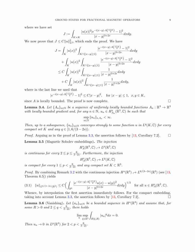
GROUND STATES FOR FRACTIONAL MAGNETIC OPERATORS 9
where we have set
J :=
∫K×K
|u(x)|2|e−i(x−y)·A(x+y2 ) − 1|2
|x− y|3+2sdxdy.
We now prove that J ≤ C‖u‖2L2 , which ends the proof. We have
J =
∫K|u(x)|2
∫K∩|x−y|≥1
|e−i(x−y)·A(x+y2 ) − 1|2
|x− y|3+2sdxdy
+
∫K|u(x)|2
∫K∩|x−y|≤1
|e−i(x−y)·A(x+y2 ) − 1|2
|x− y|3+2sdxdy
≤ C∫K|u(x)|2
∫K∩|x−y|≥1
1
|x− y|3+2sdxdy
+ C
∫K|u(x)|2
∫K∩|x−y|≤1
1
|x− y|1+2sdxdy,
where in the last line we used that
|e−i(x−y)·A(x+y2 ) − 1|2 ≤ C|x− y|2, for |x− y| ≤ 1, x, y ∈ K,
since A is locally bounded. The proof is now complete.
Lemma 3.4. Let Ann∈N be a sequence of uniformly locally bounded functions An : R3 → R3
with locally bounded gradient and, for any n ∈ N, un ∈ HsAn
(R3,C) be such that
supn∈N‖un‖s,An <∞.
Then, up to a subsequence, unn∈N converges strongly to some function u in Lq(K,C) for everycompact set K and any q ∈ [1, 6/(3− 2s)).
Proof. Arguing as in the proof of Lemma 3.3, the assertion follows by [13, Corollary 7.2].
Lemma 3.5 (Magnetic Sobolev embeddings). The injection
HsA(R3,C) → Lp(R3,C)
is continuous for every 2 ≤ p ≤ 63−2s . Furthermore, the injection
HsA(R3,C) → Lp(K,C)
is compact for every 1 ≤ p < 63−2s and any compact set K ⊂ R3.
Proof. By combining Remark 3.2 with the continuous injection Hs(R3) → L6/(3−2s)(R3) (see [13,Theorem 6.5]) yields
(3.1) ‖u‖L6/(3−2s)(R3) ≤ C(∫
R6
|e−i(x−y)·A(x+y2 )u(x)− u(y)|2
|x− y|3+2sdxdy
)1/2for all u ∈ Hs
A(R3,C).
Whence, by interpolation the first assertion immediately follows. For the compact embedding,taking into account Lemma 3.3, the assertion follows by [13, Corollary 7.2].
Lemma 3.6 (Vanishing). Let unn∈N be a bounded sequence in Hs(R3) and assume that, forsome R > 0 and 2 ≤ q < 6
3−2s , there holds
limn
supξ∈R3
∫B(ξ,R)
|un|qdx = 0.
Then un → 0 in Lp(R3) for 2 < p < 63−2s .

10 P. D’AVENIA AND M. SQUASSINA
Proof. See [11, Lemma 2.3].
Lemma 3.7 (Localized Sobolev inequality). Let ξ ∈ R3 and R > 0. Then, for u ∈ Hs(BR(ξ)),
‖u‖L
63−2s (BR(ξ))
≤ C(s)
(1
R2s
∫BR(ξ)
|u(x)|2dx+
∫BR(ξ)×BR(ξ)
|u(x)− u(y)|2
|x− y|3+2sdydx
)1/2
for some constant C(s) > 0. In particular for every 1 ≤ p ≤ 63−2s there holds
‖u‖Lp(BR(ξ)) ≤ C(s,R)‖u‖Hs(BR(ξ))
for some constant C(s,R) > 0 and all u ∈ Hs(BR(ξ)).
Proof. See [4, Proposition 2.5] for the first inequality. The second inequality immediately follows.
Lemma 3.8 (Cut-off estimates). Let u ∈ HsA(R3,C) and ϕ ∈ C0,1(R3) with 0 ≤ ϕ ≤ 1. Then,
for every pair of measurable sets E1, E2 ⊂ R3, we have∫E1×E2
|e−i(x−y)·A(x+y2 )ϕ(x)u(x)− ϕ(y)u(y)|2
|x− y|3+2sdxdy ≤ C min
∫E1
|u|2dx,∫E2
|u|2dx
+ C
∫E1×E2
|e−i(x−y)·A(x+y2 )u(x)− u(y)|2
|x− y|3+2sdxdy,
where C depends on s and on the Lipschitz constant of ϕ.
Proof. The proof follows by arguing as in [13, Lemma 5.3], where the case A = 0 and E1 = E2 isconsidered. For the sake of completeness, we show the details. We have∫
E1×E2
|e−i(x−y)·A(x+y2 )ϕ(x)u(x)− ϕ(y)u(y)|2
|x− y|3+2sdxdy
≤ C∫E1×E2
|e−i(x−y)·A(x+y2 )u(x)− u(y)|2
|x− y|3+2sdxdy + C
∫E1×E2
|u(y)|2|ϕ(x)− ϕ(y)|2
|x− y|3+2sdxdy.
On the other hand, the second integral splits as∫E2
|u(y)|2∫E1∩|x−y|≤1
1
|x− y|1+2sdxdy+
∫E2
|u(y)|2∫E1∩|x−y|≥1
1
|x− y|3+2sdxdy ≤ C
∫E2
|u|2dy.
Analogously, we have∫E1×E2
|ϕ(x)u(x)− ei(x−y)·A(x+y2 )ϕ(y)u(y)|2
|x− y|3+2sdxdy
≤ C∫E1×E2
|e−i(x−y)·A(x+y2 )u(x)− u(y)|2
|x− y|3+2sdxdy + C
∫E1×E2
|u(x)|2|ϕ(x)− ϕ(y)|2
|x− y|3+2sdxdy,
and the second term can be estimated as before by∫E1|u|2dx. The assertion follows.
Thus we can prove
Lemma 3.9 (Dicothomy). Let unn∈N be a sequence in HsA(R3,C) such that, for some L > 0,
‖un‖Lp(R3) = 1, limn‖un‖2s,A = L,
and let us set
µn(x) = |un(x)|2 +
∫R3
|e−i(x−y)·A(x+y2 )un(x)− un(y)|2
|x− y|3+2sdy, x ∈ R3, n ∈ N.

GROUND STATES FOR FRACTIONAL MAGNETIC OPERATORS 11
Assume that there exists β ∈ (0, L) such that for all ε > 0 there exist R > 0, n ≥ 1, a sequenceof radii Rn → +∞ and ξnn∈N ⊂ R3 such that for n ≥ n∣∣∣∣∫
R3
µ1n(x)dx− β
∣∣∣∣ ≤ ε, µ1n := 1BR(ξn)µn,∣∣∣∣∫
R3
µ2n(x)dx− (L− β)
∣∣∣∣ ≤ ε, µ2n := 1BcRn (ξn)µn,∫
R3
|µn(x)− µ1n(x)− µ2
n(x)|dx ≤ ε.(3.2)
Then there exist u1nn∈N, u2
nn∈N ⊂ HsA(R3,C) such that dist(supp(u1
n), supp(u2n))→ +∞ and∣∣‖u1
n‖2s,A − β∣∣ ≤ ε,(3.3) ∣∣‖u2
n‖2s,A − (L− β)∣∣ ≤ ε,(3.4)
‖un − u1n − u2
n‖s,A ≤ ε,(3.5) ∣∣∣1− ‖u1n‖
pLp(R3)
− ‖u2n‖
pLp(R3)
∣∣∣ ≤ ε(3.6)
for any n ≥ n.
Proof. Notice that we have∫R3
µ1ndx =
∫BR(ξn)
|un|2dx+
∫BR(ξn)×BR(ξn)
|e−i(x−y)·A(x+y2 )un(x)− un(y)|2
|x− y|3+2sdxdy
+
∫BR(ξn)×Bc
R(ξn)
|e−i(x−y)·A(x+y2 )un(x)− un(y)|2
|x− y|3+2sdxdy,
(3.7)
as well as∫R3
µ2ndx =
∫BcRn (ξn)
|un|2dx+
∫BcRn (ξn)×BcRn (ξn)
|e−i(x−y)·A(x+y2 )un(x)− un(y)|2
|x− y|3+2sdxdy
+
∫BcRn (ξn)×BRn (ξn)
|e−i(x−y)·A(x+y2 )un(x)− un(y)|2
|x− y|3+2sdxdy,
and, from inequality (3.2), we have, for n ≥ n,∫R≤|x−ξn|≤Rn×R3
|e−i(x−y)·A(x+y2 )un(x)− un(y)|2
|x− y|3+2sdxdy ≤ ε,(3.8)
∫R3×R≤|y−ξn|≤Rn
|e−i(x−y)·A(x+y2 )un(x)− un(y)|2
|x− y|3+2sdxdy ≤ ε,(3.9) ∫
R≤|x−ξn|≤Rn|un|2dx ≤ ε.(3.10)
For every r > 0, let ϕr ∈ C∞(R3) be a radially symmetric function such that ϕr = 1 on Br(0)and ϕr = 0 su Bc
2r(0). In light of Lemma 3.8 applied with E1 = E2 = R3, for any n ∈ N, we canconsider the functions
u1n := ϕR(· − ξn)un ∈ Hs
A(R3,C), u2n := (1− ϕRn/2(· − ξn))un ∈ Hs
A(R3,C).
We observe for further usage that the functions ϕR(· − ξn) and 1−ϕRn/2(· − ξn) have a Lipschitz
constant which is uniformly bounded with respect to n. Moreover, dist(supp(u1n), supp(u2
n))→∞.

12 P. D’AVENIA AND M. SQUASSINA
Let us consider u1nn∈N. We have [u1
n]2s,A =∑5
i=1 Iin, where
I1n :=
∫BR(ξn)×BR(ξn)
|e−i(x−y)·A(x+y2 )un(x)− un(y)|2
|x− y|3+2sdxdy,
I2n :=
∫B2R(ξn)\BR(ξn)×B2R(ξn)\BR(ξn)
|e−i(x−y)·A(x+y2 )u1
n(x)− u1n(y)|2
|x− y|3+2sdxdy,
I3n := 2
∫B2R(ξn)\BR(ξn)×BR(ξn)
|e−i(x−y)·A(x+y2 )u1
n(x)− u1n(y)|2
|x− y|3+2sdxdy,
I4n := 2
∫B2R(ξn)\BR(ξn)×Bc
2R(ξn)
|e−i(x−y)·A(x+y2 )u1
n(x)− u1n(y)|2
|x− y|3+2sdxdy,
I5n := 2
∫BR(ξn)×Bc
2R(ξn)
|e−i(x−y)·A(x+y2 )u1
n(x)− u1n(y)|2
|x− y|3+2sdxdy.
Concerning Iin with i = 2, 3, 4, since for suitable measurable sets Ei2 ⊂ R3 and ci > 0,
Iin = ci
∫B2R(ξn)\BR(ξn)×Ei2
|e−i(x−y)·A(x+y2 )u1
n(x)− u1n(y)|2
|x− y|3+2sdxdy,
in light of Lemma 3.8 and inequalities (3.8)-(3.10), we have
Iin ≤ C
[∫B2R(ξn)\BR(ξn)
|un|2dx+
∫B2R(ξn)\BR(ξn)×Ei2
|e−i(x−y)·A(x+y2 )un(x)− un(y)|2
|x− y|3+2sdxdy
]≤ Cε,
(3.11)
being B2R(ξn) \BR(ξn) ⊂ R ≤ |x− ξn| ≤ Rn for every n large enough.Concerning I5
n, we have
I5n = 2
∫BR(ξn)×2R≤|y−ξn|≤Rn
|e−i(x−y)·A(x+y2 )u1
n(x)− u1n(y)|2
|x− y|3+2sdxdy
+ 2
∫BR(ξn)×BcRn (ξn)
|e−i(x−y)·A(x+y2 )u1
n(x)− u1n(y)|2
|x− y|3+2sdxdy.
Then, arguing as in (3.11) for Iin (i = 2, 3, 4) we get∫BR(ξn)×2R≤|y−ξn|≤Rn
|e−i(x−y)·A(x+y2 )u1
n(x)− u1n(y)|2
|x− y|3+2sdxdy ≤ Cε,
for large n. On the other hand, as far as the second term in concerned, we get∫BR(ξn)×BcRn (ξn)
|e−i(x−y)·A(x+y2 )u1
n(x)− u1n(y)|2
|x− y|3+2sdxdy =
∫BR(ξn)×BcRn (ξn)
|un(x)|2
|x− y|3+2sdxdy,

GROUND STATES FOR FRACTIONAL MAGNETIC OPERATORS 13
since u1n(y) = 0 for all y ∈ Bc
Rn(ξn) and u1
n(x) = un(x) for all x ∈ BR(ξn). Observe first that if
(x, y) ∈ BR(ξn)×BcRn
(ξn), then |x− y| ≥ Rn − R→∞, as n→∞. We thus have∫BR(ξn)×BcRn (ξn)
|un(x)|2
|x− y|3+2sdxdy
≤ 1
(Rn − R)δ
∫BR(ξn)
|un(x)|2(∫|x−y|≥1
1
|x− y|3+2s−δ dy
)dx ≤ C
(Rn − R)δ≤ Cε,
(3.12)
where 0 < δ < 2s. Here we have used the boundedness of unn∈N in L2(R3,C). So we have that[u1n]2s,A = I1
n + ςn,ε with ςn,ε ≤ Cε for n large, which implies on account of (3.10)
(3.13) ‖u1n‖2s,A =
∫BR(ξn)
|un|2dx+ I1n + ςn,ε, ςn,ε ≤ Cε.
A similar argument involving unn∈N in place of u1nn∈N shows that formula (3.7) writes as
(3.14)
∫R3
µ1ndx =
∫BR(ξn)
|un|2dx+ I1n + ςn,ε, ςn,ε ≤ Cε.
Indeed, since∫BR(ξn)×Bc
R(ξn)
|e−i(x−y)·A(x+y2 )un(x)− un(y)|2
|x− y|3+2sdxdy
≤∫BR(ξn)×R≤|y−ξn|≤Rn
|e−i(x−y)·A(x+y2 )un(x)− un(y)|2
|x− y|3+2sdxdy
+ C
[∫BR(ξn)×BcRn (ξn)
|un(x)|2
|x− y|3+2sdxdy +
∫BR(ξn)×BcRn (ξn)
|un(y)|2
|x− y|3+2sdxdy
],
by (3.9) and arguing as in (3.12) we can conclude. By combining (3.13) and (3.14) we finallyobtain the desired estimate (3.3).
Now, concerning u2nn∈N, we have [u2
n]2s,A =∑5
i=1 Jin, where we have set
J1n :=
∫BcRn (ξn)×BcRn (ξn)
|e−i(x−y)·A(x+y2 )un(x)− un(y)|2
|x− y|3+2sdxdy,
J2n :=
∫BRn (ξn)\BRn/2(ξn)×BRn (ξn)\BRn/2(ξn)
|e−i(x−y)·A(x+y2 )u2
n(x)− u2n(y)|2
|x− y|3+2sdxdy,
J3n := 2
∫BRn (ξn)\BRn/2(ξn)×BRn/2(ξn)
|e−i(x−y)·A(x+y2 )u2
n(x)− u2n(y)|2
|x− y|3+2sdxdy,
J4n := 2
∫BRn (ξn)\BRn/2(ξn)×BcRn (ξn)
|e−i(x−y)·A(x+y2 )u2
n(x)− u2n(y)|2
|x− y|3+2sdxdy,
J5n := 2
∫BRn/2(ξn)×BcRn (ξn)
|e−i(x−y)·A(x+y2 )u2
n(x)− u2n(y)|2
|x− y|3+2sdxdy.
Concerning J in with i = 2, 3, 4, observe that the integration domains are BRn(ξn)\BRn/2(ξn)×Ei2,
for suitable measurable Ei2’s, and they are subset of R ≤ |x− ξn| ≤ Rn × R3 for n sufficiently

14 P. D’AVENIA AND M. SQUASSINA
large. Thus we can argue as in (3.11). Finally, J5n can be estimated with similar arguments to
that used in (3.12) and, as for µ1n, using also (3.10), we obtain∫
R3
µ2n(x)dx =
∫BcRn (ξn)
|un|2dx+ J1n + ςn,ε, ςn,ε ≤ Cε.
By combining all these estimates we get (3.4) for any n large.Conclusion (3.5) follows by (3.8)-(3.10). In fact, setting
vn := un − u1n − u2
n = (ϕRn/2(· − ξn)− ϕR(· − ξn))un,
for all n, inequality (3.10) yields∫R3
|vn|2dx =
∫R3
(ϕRn/2(x− ξn)− ϕR(x− ξn))2|un|2dx ≤∫R≤|x−ξn|≤Rn
|un|2dx ≤ ε.
Furthermore, [vn]2s,A =∑4
i=1Kin, where
K1n :=
∫BRn (ξn)\BR(ξn)×BRn (ξn)\BR(ξn)
|e−i(x−y)·A(x+y2 )vn(x)− vn(y)|2
|x− y|3+2sdxdy,
K2n := 2
∫BRn (ξn)\BR(ξn)×BR(ξn)
|e−i(x−y)·A(x+y2 )vn(x)− vn(y)|2
|x− y|3+2sdxdy,
K3n := 2
∫BRn (ξn)\BR(ξn)×BcRn (ξn)
|e−i(x−y)·A(x+y2 )vn(x)− vn(y)|2
|x− y|3+2sdxdy.
Since vn = ϕun with ϕ := (ϕRn/2(· − ξn)− ϕR(· − ξn)), we can repeat the arguments performedin (3.11). Concerning the final assertion (3.6), we have for some ϑ > 0,
1− ‖u1n‖
pLp − ‖u
2n‖
pLp =
∫R3
(1− ϕp
R(x− ξn)− (1− ϕRn/2(x− ξn))p
)|un|pdx
≤∫R≤|x−ξn|≤Rn
|un|pdx
≤(∫R≤|x−ξn|≤Rn
|un|2dx)ϑp
2(∫
R3
|un|6
3−2sdx) (1−ϑ)p(3−2s)
6
≤ ε,
in light of (3.10) and Lemma 3.5. This concludes the proof.
Lemma 3.10 (Partial Gauge invariance). Let ξ ∈ R3 and u ∈ HsA(R3,C). For η ∈ R3, let us set
v(x) = eiη·xu(x+ ξ), x ∈ R3.
Then v ∈ HsAη
(R3,C) and
‖u‖s,A = ‖v‖s,Aη , where Aη := A(·+ ξ) + η.
Proof. Of course ‖v‖L2 = ‖u‖L2 . Moreover, a change of variables yields∫R6
|e−i(x−y)·Aη(x+y2 )v(x)− v(y)|2
|x− y|3+2sdxdy =
∫R6
|e−i(x−y)·A(x+y2
+ξ)u(x+ ξ)− u(y + ξ)|2
|x− y|3+2sdxdy
=
∫R6
|e−i(x−y)·A(x+y2 )u(x)− u(y)|2
|x− y|3+2sdxdy,
which yields the assertion.

GROUND STATES FOR FRACTIONAL MAGNETIC OPERATORS 15
If A is linear, then, taking η = −A(ξ) in Lemma 3.10, we get Aη = A and hence
Lemma 3.11 (Partial Gauge invariance). Let ξ ∈ R3 and u ∈ HsA(R3,C). Assume that A is
linear and let us set
v(x) = e−iA(ξ)·xu(x+ ξ), x ∈ R3.
Then v ∈ HsA(R3,C) and ‖u‖s,A = ‖v‖s,A.
4. Existence of minimizers
Let 2 < p < 6/(3 − 2s) and consider the minimization problem (MA). First of all observe thatby Sobolev embedding, MA > 0. Once a solution to (MA) exists, due to the Lagrange MultiplierTheorem, there is λ ∈ R such that
cs2<∫R6
(e−i(x−y)·A(x+y
2 )u(x)− u(y))(e−i(x−y)·A(x+y
2 )v(x)− v(y))
|x− y|3+2sdxdy
+ <∫R3
uvdx = λ<∫R3
|u|p−2uvdx, for all v ∈ HsA(R3,C).
A multiple of u removes the Lagrange multiplier λ and provides a weak solution to (Ps,A).Moreover, if we set
MA(λ) := infu∈S (λ)
‖u‖2s,A,
where
S (λ) :=
u ∈ Hs
A(R3,C) :
∫R3
|u|pdx = λ
,
we have that for every λ > 0
(4.1) MA(λ) = λ2pMA.
4.1. Subcritical symmetric case. Let 2 < p < 63−2s and consider the problem
MA,r = infu∈Sr
‖u‖2s,A,
where
Sr =
u ∈ Hs
A,rad(R3,C) :
∫R3
|u|pdx = 1
.
First we give the following preliminary result.
Lemma 4.1 (Compact radial embedding). For every 2 < q < 6/(3− 2s), the mapping
HsA,rad(R3,C) 3 u 7→ |u| ∈ Lq(R3),
is compact.
Proof. By Lemma 3.1, namely the Diamagnetic inequality, we know that the mapping
HsA(R3,C) 3 u 7→ |u| ∈ Hs(R3,R),
is continuous. Then, the assertion follows directly by [24, Theorem II.1].
We are ready to prove (i) of Theorem 1.2
Theorem 4.2 (Existence of radial minimizers). For any 2 < p < 6/(3 − 2s), the minimizationproblem MA,r admits a solution. In particular, there exists a nontrivial radially symmetric weaksolution u ∈ Hs
A,rad(R3,C) to the problem (Ps,A).

16 P. D’AVENIA AND M. SQUASSINA
Proof. Let unn∈N ⊂ Sr be a minimizing sequence for MA,r, namely ‖un‖Lp(R3) = 1 for all n
and ‖un‖2s,A →MA,r, as n→∞. Then, up to a subsequence, it converges weakly to some radialfunction u. On account of Lemma 3.5, un → u a.e. up to a subsequence. By Lemma 4.1, up toa subsequence |un|n∈N converges strongly to some v in Lq(R3) for every 2 < q < 6/(3 − 2s).Of course, v = |u| by pointwise convergence. In particular we can pass to the limit into theconstraint ‖un‖Lp(R3) = 1 to get ‖u‖Lp(R3) = 1. Then u is a solution to MA,r, since by virtue ofFatou Lemma
MA,r ≤∫R3
|u(x)|2dx+
∫R6
|e−i(x−y)·A(x+y2 )u(x)− u(y)|2
|x− y|3+2sdxdy
≤ lim infn
(∫R3
|un(x)|2dx+
∫R6
|e−i(x−y)·A(x+y2 )un(x)− un(y)|2
|x− y|3+2sdxdy
)= MA,r.
This concludes the proof.
4.2. Subcritical case. In this subsection we study the minimization problem (MA) in the case2 < p < 6
3−2s .
4.2.1. Constant magnetic field case. Let us consider (MA) under the assumption that A : R3 →R3 is linear. The local case was extensively studied in [15] for the magnetic potential
A(x1, x2, x3) =b
2(−x2, x1, 0), b ∈ R \ 0.
Hence we can prove (ii) of Theorem 1.2.
Theorem 4.3 (Existence of minimizers, I). Assume that the potential A : R3 → R3 is linear.Then, for any 2 < p < 6
3−2s the minimization problem (MA) admits a solution.
Proof. Let unn∈N ⊂ S be a minimizing sequence for MA, namely ‖un‖Lp = 1 for all n and‖un‖2s,A → MA, as n → ∞. We want to develop a concentration compactness argument [25] onthe measure of density defined by
µn(x) := |un(x)|2 +
∫R3
|e−i(x−y)·A(x+y2 )un(x)− un(y)|2
|x− y|3+2sdy, x ∈ R3, n ∈ N.
Notice that µnn∈N ⊂ L1(R3) and, since ‖un‖2s,A = MA + on(1),
supn∈N
∫R3
µn(x)dx <∞.
More precisely, we shall apply [25, Lemma I.1] by taking ρn = µn. Only vanishing, dichotomyor tightness (yielding compactness) are possible. Vanishing can be ruled out. In fact, assume bycontradiction that, for all R > 0 fixed, there holds
limn
supξ∈RN
∫BR(ξ)
µn(x)dx = 0,
namely
limn
supξ∈RN
(∫BR(ξ)
|un(x)|2dx+
∫BR(ξ)×R3
|e−i(x−y)·A(x+y2 )un(x)− un(y)|2
|x− y|3+2sdxdy
)= 0.
By Remark 3.2 it follows that
limn
supξ∈RN
(∫BR(ξ)
|un(x)|2dx+
∫BR(ξ)×R3
||un(x)| − |un(y)||2
|x− y|3+2sdxdy
)= 0.

GROUND STATES FOR FRACTIONAL MAGNETIC OPERATORS 17
In particular, we get
limn
supξ∈RN
‖|un|‖2Hs(BR(ξ)) = 0
and this implies, by virtue of Lemma 3.7, that for any R > 0
limn
supξ∈RN
∫BR(ξ)
|un(x)|pdx = 0.
Thus, in light of Lemma 3.6, un → 0 in Lp which violates the constraint ‖un‖Lp = 1. Whence,vanishing cannot occur.We now exclude the dicothomy. According to [25, Lemma I.1], this, precisely, means that thereexists β ∈ (0,MA) such that for all ε > 0 there are R > 0, n ≥ 1, a sequence of radii Rn → +∞and ξnn∈N ⊂ R3 such that for n ≥ n∣∣∣∣∫
R3
µ1n(x)dx− β
∣∣∣∣ ≤ ε, µ1n(x) := 1BR(ξn)µn,∣∣∣∣∫
R3
µ2n(x)dx− (MA − β)
∣∣∣∣ ≤ ε, µ2n(x) := 1BcRn (ξn)µn,∫
R3
|µn(x)− µ1n(x)− µ2
n(x)|dx ≤ ε.
Then, by virtue of Lemma 3.9, there exist two sequences u1nn∈N, u2
nn∈N ⊂ HsA(R3,C) such
that dist(supp(u1n), supp(u2
n))→ +∞ and∣∣‖u1n‖2s,A − β
∣∣ ≤ ε,(4.2) ∣∣‖u2n‖2s,A − (MA − β)
∣∣ ≤ ε,(4.3) ∣∣1− ‖u1n‖
pLp − ‖u
2n‖
pLp
∣∣ ≤ ε,(4.4)
for any n ≥ n. Up to a subsequence, in view of (4.4), there exist ϑε, ωε ∈ (0, 1) such that
‖u1n‖
pLp =: ϑn,ε → ϑε, ‖u2
n‖pLp =: ωn,ε → ωε, |1− ϑε − ωε| ≤ ε, as n→∞.
Notice that ϑε does not converge to 1 as ε→ 0, otherwise by (4.1) and (4.2), for ε small we get
β + ε ≥ lim supn‖u1
n‖2s,A ≥ lim supn
MA(ϑn,ε) = MAϑ2/pε > β + ε.
Of course ϑε does not converge to 0 either, as ε→ 0, otherwise ωε → 1 and a contradiction wouldagain follow by arguing as above on u2
n and using (4.3). Whence, by means of (4.1), (4.2), (4.3),
and since λ2/p + (1− λ)2/p > 1 for any λ ∈ (0, 1), if ε is small enough
MA + 2ε ≥ lim supn
(‖u1
n‖2s,A + ‖u2n‖2s,A
)≥ lim sup
n(MA(ϑn,ε) + MA(ωn,ε))
= MA
(ϑ2/pε + ω2/p
ε
)> MA + 2ε,
a contradiction. This means that tightness needs to occur, namely there exists a sequence ξnn∈Nsuch that for all ε > 0 there exists R > 0 with∫
BcR(ξn)|un(x)|2dx+
∫BcR(ξn)×R3
|e−i(x−y)·A(x+y2 )un(x)− un(y)|2
|x− y|3+2sdxdy < ε
for any n. In particular, setting un(x) := un(x+ ξn), for all ε > 0 there is R > 0 such that
(4.5) supn∈N
∫BcR(0)
|un(x)|2dx < ε.

18 P. D’AVENIA AND M. SQUASSINA
Let us consider
vn(x) := e−iA(ξn)·xun(x), x ∈ R3.
Since, by Lemma 3.11, ‖vn‖s,A = ‖un‖s,A, we have that vnn∈N is bounded in HsA(R3,C). Notice
also that, since |vn(x)| = |un(x)| for a.e. x ∈ R3 and any n ∈ N, by (4.5) we have that for allε > 0 there is R > 0 such that
(4.6) supn∈N
∫BcR(0)
|vn(x)|2dx < ε.
Thus, in view of the compact injection provided by Lemma 3.5, up to a subsequence, vnn∈Nconverges weakly, strongly in L2(BR(0),C) and point-wisely to some function v. Moreover, by(4.6), it follows that vn → v strongly in L2(R3,C) as well as in Lq(R3,C) for any 2 < q < 6/(3−2s),via interpolation. Hence ‖v‖Lp = 1. Hence, by Fatou’s lemma, we have
MA ≤ ‖v‖2s,A ≤ lim infn‖vn‖2s,A = lim inf
n‖un‖2s,A = MA,
which proves the existence of a minimizer.
4.2.2. Variable magnetic field case. We now prove (iii) of Theorem 1.2.
Theorem 4.4 (Existence of minimizers, II). Assume that the potential A : R3 → R3 satisfiesassumption A and that
(4.7) MA < infΞ∈X
MAΞ.
Then, for any 2 < p < 63−2s , the minimization problem (MA) admits a solution.
Proof. By arguing as in the proof of Theorem 4.3, if unn∈N is a minimizing sequence for MA,we can find a sequence ξnn∈N such that for all ε > 0 there exists R > 0 with∫
BcR(ξn)|un(x)|2dx+
∫BcR(ξn)×R3
|e−i(x−y)·A(x+y2 )un(x)− un(y)|2
|x− y|3+2sdxdy < ε
for any n. In particular, setting again un(x) := un(x+ ξn), for all ε > 0 there is R > 0 such that
supn∈N
∫BcR(0)
|un(x)|2dx < ε.
Assume by contradiction that the sequence ξnn∈N is unbounded. Then, since A satisfies con-dition A , there exists a sequence Hnn∈N ⊂ R3 such that (1.4) holds. We thus consider thesequence
vn(x) := eiHn·xun(x), x ∈ R3.
By virtue of Lemma 3.10 it follows that
supn∈N‖vn‖s,An = sup
n∈N‖un‖s,A <∞, An(x) = A(x+ ξn) +Hn.
Then, by combining Lemma 3.4 with
supn∈N
∫BcR(0)
|vn(x)|2dx < ε,
up to a subsequence, vnn∈N is strongly convergent in Lq(R3) for all q ∈ [2, 6/(3− 2s)) to somefunction v which satisfies the constraint ‖v‖Lp = 1. By combining Lemma 3.10 with Fatou’s

GROUND STATES FOR FRACTIONAL MAGNETIC OPERATORS 19
Lemma and (4.7), we get
MAΞ≤ ‖v‖2s,AΞ
=
∫R3
|v|2dx+
∫R6
|e−i(x−y)·AΞ(x+y2 )v(x)− v(y)|2
|x− y|3+2sdxdy
≤ limn
∫R3
|vn|2dx+ lim infn
∫R6
|e−i(x−y)·An(x+y2 )vn(x)− vn(y)|2
|x− y|3+2sdxdy
= limn
∫R3
|un|2dx+ lim infn
∫R6
|e−i(x−y)·A(x+y2 )un(x)− un(y)|2
|x− y|3+2sdxdy
= MA < infΞ∈X
MAΞ≤MAΞ
,
a contradiction. Therefore, it follows that ξnn∈N is bounded. The assertion then immediatelyfollows arguing on the original sequence unn∈N.
4.3. Critical case. Let DsA(R3,C) be the completion of C∞c (R3,C) with respect to the semi-
norm [·]s,A. The functions of DsA(R3,C) satisfy the Sobolev inequality stated in formula (3.1).
The space DsA(R3,C) is a real Hilbert space with respect to the scalar product
(u, v)s,A :=cs2<∫R6
(e−i(x−y)·A(x+y
2 )u(x)− u(y))(
e−i(x−y)·A(x+y2 )v(x)− v(y)
)|x− y|3+2s
dxdy.
We consider the minimization problem (M cA). Of course, by density, we have
M cA = inf
u∈S c∩C∞c (R3,C)[u]2s,A, M c
0 = infu∈S c
0 ∩C∞c (R3,C)[u]2s,0.
where S c0 = u ∈ Ds(R3,C) : ‖u‖L6/(3−2s) = 1. Moreover, since [|u|]s,0 ≤ [u]s,0, we have
(4.8) M c0 = inf
u∈S c0 ∩C∞c (R3,R)
[u]2s,0.
Remark 4.5. It is known [7,10] that all the real valued fixed sign solutions to M c0 are given by
Uz,ε(x) = ds
(ε
ε2 + |x− z|2
) 3−2s2
for arbitrary ε > 0, z ∈ R3 and that these are also the unique fixed sign solutions to
(−∆)su = u3+2s3−2s in R3.
We now prove the following crucial lemma
Lemma 4.6. It holds M cA = M c
0 .
Proof. Let ε > 0 and u ∈ C∞c (R3,R) be such that∫R3
|u|6/(3−2s)dx = 1, [u]2s,0 ≤M c0 + ε,
in light of formula (4.8) for M c0 . Consider now the scaling
uσ(x) = σ−3−2s
2 u(xσ
), σ > 0, x ∈ R3.
It is readily checked that∫R3
|uσ|6/(3−2s)dx =
∫R3
|u|6/(3−2s)dx = 1, [uσ]s,0 = [u]s,0, for all σ > 0.

20 P. D’AVENIA AND M. SQUASSINA
There holds that
[uσ]2s,A =
∫R6
|e−iσ(x−y)·A(σ x+y2 )u(x)− u(y)|2
|x− y|3+2sdxdy.
Then, we compute
[uσ]2s,A − [u]2s,0 =
∫R6
|e−iσ(x−y)·A(σ x+y2 )u(x)− u(y)|2 − |u(x)− u(y)|2
|x− y|3+2sdxdy
=
∫R6
Θσ(x, y)dxdy =
∫K×K
Θσ(x, y)dxdy,
where K is the compact support of u and
Θσ(x, y) :=2<((
1− e−iσ(x−y)·A(σ x+y2 ))u(x)u(y)
)|x− y|3+2s
=2(1− cos
(σ(x− y) ·A
(σ x+y
2
)))u(x)u(y)
|x− y|3+2s,
a.e. in R6. Of course Θσ(x, y)→ 0 for a.e. (x, y) ∈ R6 as σ → 0. Since A is locally bounded then
1− cos(σ(x− y) ·A
(σx+ y
2
))≤ C|x− y|2 x, y ∈ K.
Therefore, since u is bounded, it follows that for some C > 0
|Θσ(x, y)| ≤ C
|x− y|1+2s, for x, y ∈ K with |x− y| < 1,
|Θσ(x, y)| ≤ C
|x− y|3+2s, for x, y ∈ K with |x− y| ≥ 1.
Then overall, we have
|Θσ(x, y)| ≤ w(x, y), w(x, y) = C min
1
|x− y|1+2s,
1
|x− y|3+2s
for x, y ∈ K,
for a suitable constant C > 0. Notice that w ∈ L1(K ×K), since∫K×K
w(x, y)dxdy =
∫(K×K)∩|x−y|<1
w(x, y)dxdy +
∫(K×K)∩|x−y|≥1
w(x, y)dxdy
≤ C∫|z|<1
1
|z|1+2sdz + C
∫|z|≥1
1
|z|3+2sdz <∞.
Then, by the Dominated Convergence Theorem, we obtain
M cA ≤ lim
σ→0[uσ]2s,A = [u]2s,0 ≤M c
0 + ε,
hence M cA ≤ M c
0 by the arbitrariness of ε. Since the opposite inequality is trivial through theDiamagnetic inequality, the desired assertion follows.
Thus we can prove (i) of Theorem 1.3.
Theorem 4.7 (Representation of solutions). Assume that M cA admits a solutions u ∈ Ds
A(R3,C).Then there exist z ∈ R3, ε > 0 and a function ϑA : R3 → R such that
u(x) = ds
(ε
ε2 + |x− z|2
) 3−2s2
eiϑA(x), x ∈ R3.

GROUND STATES FOR FRACTIONAL MAGNETIC OPERATORS 21
Proof. If u ∈ DsA(R3,C) is a solution to M c
A, then by the Diamagnetic inequality and Lemma 4.6,
M cA = M c
0 ≤ [|u|]2s,0 ≤ [u]2s,A = M cA.
Then, it follows that M c0 = [|u|]2s,0, which implies the assertion by Remark 4.5.
For a function u ∈ DsA(R3,C) we define ΥA
u : R6 → R by setting
ΥAu (x, y) := 2<
(|u(x)||u(y)| − e−i(x−y)·A
(x+y
2
)u(x)u(y)
), a.e. in R6.
Finally we have
Theorem 4.8 (Nonexistence). Assume that for a function u ∈ DsA(R3,C) we have
(4.9) ΥAu (x, y) > 0 on E ⊂ R6 with L6(E) > 0.
Then u cannot be a solution to problem M cA.
Proof. For every u ∈ DsA(R3,C) we have |u| ∈ Ds(R3) and there holds
[u]2s,A − [|u|]2s,0 =
∫R6
ΥAu (x, y)dxdy.
Assume by contradiction that u solves M cA. Then, since ‖u‖L6/(3−2s) = 1, by Lemma 4.6 and
assumption (4.9), we conclude that M c0 = M c
A = [u]2s,A > [|u|]2s,0 ≥M c0 , a contradiction.
As a consequence we get (ii) of Theorem 1.3.
Corollary 4.9 (Nonexistence of constant phase solutions). Assume that
(x− y) ·A(x+ y) 6≡ kπ, for some k ∈ N and on some E ⊂ R6 with L6(E) > 0.
Then M cA does not admit solutions u ∈ Ds
A(R3,C) of the form u(x) = eiϑv(x) for some ϑ ∈ Rand v ∈ Ds
A(R3,R) of fixed sign.
Proof. Assumption (4.9) is fulfilled, since
ΥAu (x, y) = 2
(1− cos
((x− y) ·A
(x+ y
2
)))v(x)v(y) > 0, for a.e. (x, y) ∈ E.
Hence, the assertion follows from Theorem 4.8.
References
[1] A. Applebaum, Levy processes and Stochastic Calculus, Cambridge Studies in Advanced Mathematics 116,Cambridge University Press, Cambridge, 2009. 2
[2] G. Arioli, A. Szulkin, A semilinear Schrodinger equation in the presence of a magnetic field, Arch. Ration.Mech. Anal. 170 (2003), 277–295. 2
[3] J. Avron, I. Herbst, B. Simon, Schrodinger operators with magnetic fields. I. General interactions, Duke Math.J. 45 (1978), 847–883. 2
[4] L. Brasco, E. Parini, The second eigenvalue of the fractional p-Laplacian, Adv. Calc. Var. 9 (2016), 323–355.10
[5] J. Bourgain, H. Brezis and P. Mironescu, Another look at Sobolev spaces, in Optimal Control and PartialDifferential Equations. A Volume in Honor of Professor Alain Bensoussan’s 60th Birthday (eds. J. L. Menaldi,E. Rofman and A. Sulem), IOS Press, Amsterdam, 2001, 439–455. 2, 8
[6] J. Bourgain, H. Brezis and P. Mironescu, Limiting embedding theorems for W s,p when s ↑ 1 and applications,J. Anal. Math. 87 (2002), 77–101. 2, 8
[7] W. Chen, C. Li, B. Ou, Classification of solutions for an integral equation, Comm. Pure Appl. Math. 59(2006), 330–343. 19
[8] S. Cingolani, S. Secchi, Semiclassical limit for nonlinear Schrodinger equations with electromagnetic fields, J.Math. Anal. Appl. 275 (2002), 108–130. 2

22 P. D’AVENIA AND M. SQUASSINA
[9] R. Cont, P. Tankov, Financial modeling with jump processes, Chapman & Hall/CRC Financial MathematicsSeries, Chapman & Hall/CRC, Boca Raton, FL, 2004. 2
[10] A. Cotsiolis, N.K. Tavoularis, Best constants for Sobolev inequalities for higher order fractional derivatives, J.Math. Anal. Appl. 295 (2004), 225–236. 19
[11] P. d’Avenia, G. Siciliano, M. Squassina, On fractional Choquard equations, Math. Models Methods Appl. Sci.25 (2015), 1447–1476. 10
[12] J. Di Cosmo, J. Van Schaftingen, Semiclassical stationary states for nonlinear Schrodinger equations under astrong external magnetic field, J. Differential Equations 259 (2015), 596–627. 2
[13] E. Di Nezza, G. Palatucci, E. Valdinoci, Hitchhiker’s guide to the fractional Sobolev spaces, Bull. Sci. Math.136 (2012), 521–573. 9, 10
[14] S. Dipierro, G. Palatucci, E. Valdinoci, Existence and symmetry results for a Schrodinger type problem involvingthe fractional Laplacian, Le Matematiche 68 (2013), 201–216. 4
[15] M. Esteban, P.L. Lions, Stationary solutions of nonlinear Schrodinger equations with an external magneticfield, Partial differential equations and the calculus of variations, Vol. I, 401–449, Progr. Nonlinear DifferentialEquations Appl. 1, Birkhauser Boston, Boston, MA, 1989. 2, 4, 16
[16] R.L. Frank, E.H. Lieb, R. Seiringer, Hardy-Lieb-Thirring inequalities for fractional Schrodinger operators, J.Amer. Math. Soc. 21 (2008), 925–950. 2
[17] T. Ichinose, Essential selfadjointness of the Weyl quantized relativistic Hamiltonian, Ann. Inst. H. PoincarePhys. Theor. 51 (1989), 265–297. 2
[18] T. Ichinose, Magnetic relativistic Schrodinger operators and imaginary-time path integrals, Mathematicalphysics, spectral theory and stochastic analysis, 247–297, Oper. Theory Adv. Appl. 232, Birkhauser/SpringerBasel AG, Basel, 2013. 2, 3
[19] T. Ichinose, H. Tamura, Imaginary-time path integral for a relativistic spinless particle in an electromagneticfield, Comm. Math. Phys. 105 (1986), 239–257. 2
[20] V. Iftimie, M. Mantoiu, R. Purice, Magnetic pseudodifferential operators, Publ. Res. Inst. Math. Sci. 43 (2007),585–623. 2
[21] K. Kurata, Existence and semi-classical limit of the least energy solution to a nonlinear Schrodinger equationwith electromagnetic fields, Nonlinear Anal. 41 (2000), 763–778. 2
[22] N. Laskin, Fractional Schrodinger equation, Phys. Rev. E 66 (2002), 056108. 2[23] E.H. Lieb, R. Seiringer, The stability of matter in quantum mechanics, Cambridge University Press, Cambridge,
2010. 2[24] P.-L. Lions, Symetrie and compacite dans le espaces de Sobolev, J. Funct. Anal 49 (1982), 315–334. 15[25] P.-L. Lions, The concentration-compactness principle in the calculus of variation. The locally compact case I,
Ann. Inst. H. Poincare Anal. Non Lineaire 1 (1984), 109–145. 16, 17[26] R. Metzler, J. Klafter, The restaurant at the random walk: recent developments in the description of anomalous
transport by fractional dynamics, J. Phys. A 37 (2004), R161–R208. 2[27] M. Reed, B. Simon, Methods of modern mathematical physics, I, Functional analysis, Academic Press, Inc.,
New York, 1980. 2[28] M. Squassina, Soliton dynamics for the nonlinear Schrodinger equation with magnetic field, Manuscripta Math.
130 (2009), 461–494. 2
(P. d’Avenia) Dipartimento di Meccanica, Matematica e ManagementPolitecnico di Bari, Via Orabona 4, I-70125 Bari, ItalyE-mail address: [email protected]
(M. Squassina) Dipartimento di Matematica e FisicaUniversita Cattolica del Sacro Cuore, Via dei Musei 41, I-25121 Brescia, ItalyE-mail address: [email protected]


![arXiv:1601.04230v2 [math.AP] 9 Nov 2016 · 2 P. D’AVENIA AND M. SQUASSINA hence the importance of the definition (1.1). Moreover, the fractional Laplacian (1.1) allows to develop](https://img.pdfslide.us/doc/110x75/5c6f604c09d3f29e208c1454/arxiv160104230v2-mathap-9-nov-2016-2-p-davenia-and-m-squassina-hence.jpg)