Embed Size (px)
Citation preview
Novel Heuristic and Metaheuristic
Approaches to Cutting and Packing
by Glenn Whitwell, BSc
Thesis Submitted to the University of Nottingham
for the degree of Doctor of Philosophy
School of Computer Science and Information Technology
September 2004

Table of Contents
TABLE OF CONTENTS
List of Figures..............................................................................................................................vi List of Tables ...............................................................................................................................xi Abstract......................................................................................................................................xiv Publications Produced ............................................................................................................... xv Acknowledgements ...................................................................................................................xvi
PART A – CUTTING AND PACKING 1
1 Introduction..........................................................................................................................2
1.1 Background and Motivation.........................................................................................2
1.2 Aims and Scope ...........................................................................................................4
1.3 Contributions................................................................................................................6
1.4 Overview of the Thesis ................................................................................................7
2 The Stock Cutting Problem ................................................................................................9
2.1 Cutting and Packing: An Overview ...........................................................................10
2.2 Two Dimensional Orthogonal Packing......................................................................17
2.3 Rectangular Benchmark Problems from the Literature .............................................32
2.4 Two Dimensional Irregular Packing ..........................................................................33
2.5 Irregular Benchmark Data from the Literature ..........................................................46
2.6 Optimisation and Search Methods .............................................................................48
2.7 Packing within Industry .............................................................................................55
2.8 Cutting and Packing: Summary .................................................................................64
ii

Table of Contents
PART B – RECTANGULAR PACKING 65
3 The Best-Fit Placement Heuristic.....................................................................................68
3.1 Overview....................................................................................................................68
3.2 Implementation ..........................................................................................................71
3.3 Benchmark Problems .................................................................................................79
3.4 Experimentation and Results .....................................................................................80
3.5 Summary ....................................................................................................................88
4 A Metaheuristic Hybrid Approach ..................................................................................89
4.1 Overview of the Hybrid Metaheuristic Approach......................................................89
4.2 Motivation of the Hybrid Strategy .............................................................................90
4.3 Development of a Floating Point Skyline Representation .........................................93
4.4 Best-Fit Conversion to Bottom-Left-Fill Representation ..........................................94
4.5 Hybrid Approach Summary.......................................................................................95
4.6 Benchmark Test Data.................................................................................................96
4.7 Experimentation and Results .....................................................................................97
4.8 Summary ..................................................................................................................112
5 An Interactive Approach ................................................................................................113
5.1 An Overview of the New User-Guided Approach...................................................113
5.2 User-Guided Procedure............................................................................................115
5.3 Benchmark Data.......................................................................................................118
5.4 Experimentation and Results ...................................................................................119
5.5 Summary ..................................................................................................................126
iii

Table of Contents
PART C – IRREGULAR PACKING 127
6 Geometry, Trigonometry and the No-Fit Polygon........................................................131
6.1 Geometry Libraries ..................................................................................................131
6.2 Shape Representation...............................................................................................132
6.3 The No-Fit Polygon .................................................................................................134
6.4 No-Fit Polygon Versus Standard Trigonometry Overlap Detection........................136
6.5 Generation of the No-Fit Polygon: Previous Literature Approaches and their
Degeneracies ............................................................................................................139
7 Automated Packing using Trigonometric Approaches ................................................149
7.1 Motivation for the Approach....................................................................................149
7.2 The New Bottom-Left-Fill Approach ......................................................................153
7.3 Benchmark Problems ...............................................................................................171
7.4 Experiments .............................................................................................................172
7.5 Summary ..................................................................................................................179
8 The No-Fit Polygon: A Robust Implementation ...........................................................180
8.1 The New No-Fit Polygon Construction Algorithm..................................................180
8.2 Orbiting / Sliding .....................................................................................................182
8.3 Start Points ...............................................................................................................191
8.4 Pseudocode ..............................................................................................................196
8.5 Problem Cases..........................................................................................................198
8.6 Generation Times on the Benchmark Data ..............................................................202
8.7 Summary ..................................................................................................................205
iv

Table of Contents
9 Automated Packing using the No-Fit Polygon ..............................................................206
9.1 Modifying the No-Fit Polygon Generation Algorithm to Handle Arcs ...................207
9.2 An Amended Packing Algorithm using the No-Fit Polygon ...................................224
9.3 Experimental Results ...............................................................................................226
9.4 Summary ..................................................................................................................235
PART D – DISCUSSION 236
10 Conclusions.......................................................................................................................237
10.1 Discussion ................................................................................................................237
10.2 Future Work .............................................................................................................243
11 Dissemination ...................................................................................................................250
11.1 Academic Community .............................................................................................250
11.2 Industrial Partner......................................................................................................252
11.3 Commercial Exploitation .........................................................................................253
REFERENCES 255
APPENDICES 275
12 APPENDIX A – Layouts for Rectangular Benchmarks ...............................................276
13 APPENDIX B – Layouts for Irregular Benchmarks ....................................................286
14 APPENDIX C – New Rectangular Benchmark Instances ............................................299
15 APPENDIX D – New Irregular Benchmark Instances.................................................308
v
List of Figures
LIST OF FIGURES
Figure 2.1. A Bottom-Left Method (Jakobs, 1996) [91].............................................................. 24
Figure 2.2. An Improved Bottom-Left Method (Liu and Teng, 1999) [93]................................ 24
Figure 2.3. Storing placement locations for one implementation of bottom-left-fill .................. 25
Figure 2.4. A comparison of the BL and BLF placement heuristics when adding a rectangle... 25
Figure 2.5. Nuances of the knife cutting procedure .................................................................... 61
Figure 2.6. Expanding shapes by ½ kerf width........................................................................... 62
Figure 3.1. Placement next to tallest neighbour.......................................................................... 70
Figure 3.2. Placement next to shortest neighbour ....................................................................... 70
Figure 3.3. Storing the skyline heights of the layout on a sheet of width 9 units when empty and
after packing seven rectangles.................................................................................. 72
Figure 3.4. Finding a new gap when the old gap has not been completely filled ....................... 74
Figure 3.5. Procedure when no rectangle will fit gap ................................................................. 75
Figure 3.6. Processing of the ‘tower’ rectangles......................................................................... 76
Figure 3.7. The solutions achieved by each of the placement policies: a) Leftmost, b) Tallest
Neighbour, and c) Smallest Neighbour on problem C2P3 from Hopper and Turton
(2001) [95]................................................................................................................ 81
Figure 3.8. The resultant packing of the best-fit heuristic with Ramesh Babu’s data. ............... 85
Figure 3.9. A comparison of the a) best-fit heuristic, b) bottom-left-fill + GA and c) bottom-
left-fill + SA using problem C7P2 from Hopper and Turton (2001) [95] ................ 85
Figure 3.10. The resultant packing from data N13 involving 3152 rectangles. A packing of
height 964 is achieved using best-fit, which is only 4 over optimum ...................... 87
Figure 4.1. General overview of the proposed hybrid approach................................................. 90
vi

List of Figures
Figure 4.2. Floating-point representation of the skyline ............................................................. 93
Figure 4.3. Conversion of best-fit’s skyline into bottom-left-fill’s placement positions ............ 94
Figure 4.4. A summary of the proposed strategy ........................................................................ 95
Figure 4.5. Two possible solutions of identical total height but vastly different skyline area
evaluations................................................................................................................ 97
Figure 4.6. Comparison graphs of the percentage above optimal when varying phase switch
parameter, m ........................................................................................................... 100
Figure 4.7. Solutions obtained by a) solitary best-fit heuristic, b) best-fit with tabu bottom-left-
fill, c) best-fit with simulated annealing bottom-left-fill and d) best-fit with genetic
algorithm bottom-left-fill on problem C5P1. ......................................................... 105
Figure 4.8. Best solutions for C7P1 (Height = 244 units) and PathP2 (Height = 103.4 units) . 106
Figure 4.9. The optimal solution found for C2P2 using tabu (height = 15 units, area = 600) .. 107
Figure 4.10. Best solutions obtained for the extended problems (from left to right): N10 (height
= 151, area = 10530), N11 (height = 152, area = 10581) and N12 (height = 304, area
= 30281) ................................................................................................................. 108
Figure 5.1. Initial solution produced by the best-fit placement heuristic (height = 124, area =
9664, eval = 244.8)................................................................................................. 115
Figure 5.2. Selection of unacceptable regions involving holes................................................. 116
Figure 5.3. Solution before (left) and after (right) metaheuristic is invoked (height = 122, area =
9636, eval = 242.45)............................................................................................... 117
Figure 5.4. Solution generated for dataset C5P1 with user interactivity (size = 72, height = 90
units, time = 11 mins)............................................................................................. 120
Figure 5.5. Example solutions generated for some of the larger problem instances using the new
interactive approach ............................................................................................... 122
Figure 6.1. The no-fit polygon of two shapes A and B............................................................. 135
Figure 6.2. Using the no-fit polygon to test for intersection between polygons A and B......... 136
vii

List of Figures
Figure 6.3. Intersection testing with the no-fit polygon............................................................ 138
Figure 6.4. No-fit polygon generation with convex shapes ...................................................... 140
Figure 6.5. Bitmap representations of non-convex pieces with a 0-1 representation or index
optimisations .......................................................................................................... 141
Figure 6.6. Convex Decompositions: a) irregular polygon, b) triangulation, c) convex division
(vertex to vertex), d) convex division (vertex to edge) .......................................... 144
Figure 6.7. a) Non-star-shaped polygon, b) Star-shaped polygon ............................................ 145
Figure 7.1. a) low resolution grid approach b) high resolution grid approach c) variable shift
approach ................................................................................................................. 151
Figure 7.2. Shape containing holes ............................................................................................ 153
Figure 7.3. Overlapping Shapes................................................................................................. 154
Figure 7.4. Line and arc x spans ................................................................................................ 156
Figure 7.5. Resolution of intersecting line primitives............................................................... 157
Figure 7.6. A line arc example where points in range are insufficient to resolve overlap........ 159
Figure 7.7. Using tangent points to resolve overlap with the line arc case ............................... 159
Figure 7.8. Resolving overlap using the tangent point method with the arc line case .............. 161
Figure 7.9. Resolving arc intersections using the points in range............................................. 162
Figure 7.10. Using the Pythagorean theorem to resolve arc intersections (method 1).............. 162
Figure 7.11. Using the Pythagorean theorem to resolve arc intersections (method 2).............. 163
Figure 7.12. Resolving a contained shape.................................................................................. 165
Figure 7.13. Contained shape and overlap is not fully resolved ................................................ 166
Figure 7.14. Density Measures ................................................................................................. 172
Figure 7.15. SWIM 100 iteration solution (6462.4 units, 607 seconds) .................................... 175
Figure 7.16. TROUSERS extended run solution (243.4 units, 3612 seconds) .......................... 177
Figure 7.17. Best solutions for Profiles1 (1377.74 units) & Profiles9 (1290.67 units) ............. 177
Figure 8.1. Initial translation of the orbiting polygon to touch the stationary polygon ............ 181
viii

List of Figures
Figure 8.2. Identification of touching edge pairs ...................................................................... 183
Figure 8.3. Translation vector: a) derived from edge a3, b) derived from edge b1 .................. 184
Figure 8.4. Touching edge-pair types ....................................................................................... 184
Figure 8.5. Two polygons touching at two separate positions and vertex-vertex touch cases... 186
Figure 8.6. Identifying the feasible angular range of translations (indicated by the arc).......... 187
Figure 8.7. Elimination of potential translation vector, a1 ....................................................... 188
Figure 8.8. Two polygons involving exactly fitting ‘passageways’ ......................................... 188
Figure 8.9. A translation vector that requires ‘trimming’ to avoid intersection........................ 189
Figure 8.10. Trimming with projections from polygon A ........................................................ 190
Figure 8.11. Interlocking concavities: a) polygons, b) no-fit polygon using sliding alone, c) the
complete no-fit polygon ......................................................................................... 191
Figure 8.12. Vertex alignment of polygon B to polygon A using edge a5: a) invalid alignment,
b) valid alignment................................................................................................... 193
Figure 8.13. Start point generation process............................................................................... 194
Figure 8.14. Multiple interlocking positions............................................................................. 198
Figure 8.15. Exact fit sliding through a “passageway”............................................................. 199
Figure 8.16. Jigsaw pieces: a) outer NFP loop, b) singular feasible internal position.............. 200
Figure 8.17. No-fit polygon of two polygons, one of which involves multiple holes .............. 201
Figure 8.18. A selection of pieces and no-fit polygons from the “Profiles 9” (letters) and
“Swim” datasets ..................................................................................................... 203
Figure 9.1. No-Fit Polygon of Two Circles .............................................................................. 208
Figure 9.2. Movement of the Touching Positions of the Circles .............................................. 208
Figure 9.3. Finding circle tangents (A and B are convex) ........................................................ 209
Figure 9.4. Creating the partial no-fit polygon circle from the arc tangents............................. 209
Figure 9.5. No arc tangent points available .............................................................................. 210
Figure 9.6. No-fit polygon of two circles in the concave case.................................................. 210
ix

List of Figures
Figure 9.7. Finding circle tangents (A is concave, B is convex) .............................................. 211
Figure 9.8. Creating the partial no-fit polygon (A is concave, B is convex) ............................ 211
Figure 9.9. Touching edges with two distinct touch positions (edge a2 and b3) ....................... 213
Figure 9.10. Non-tangential touching arcs................................................................................ 214
Figure 9.11. Potential translation vector derived in case (ii): arc B’s start/end point touches the
middle of arc A....................................................................................................... 215
Figure 9.12. Potential translation vector derived in case (ii) when a tangent point is present: arc
B’s start/end point touches the middle of arc A ..................................................... 215
Figure 9.13. Potential translation vector derived in case (iii): arc A’s start/end point touches the
middle of arc B ....................................................................................................... 216
Figure 9.14. Tangents with lines and arcs................................................................................. 217
Figure 9.15. Conversion to tangential lines at the touch point of an arc................................... 218
Figure 9.16. Two touching arcs and a potential arc translation ................................................ 219
Figure 9.17. Creating the tangential lines ................................................................................. 219
Figure 9.18. Revisiting the line method of section 8.2.3 using tangential lines ....................... 219
Figure 9.19. Tangential trimming of the feasible translation from an arc and a line, a4 and b4 221
Figure 9.20. Tangential trimming of the feasible translation from two arcs............................. 221
Figure 9.21. Annotated examples of no-fit polygons including arcs ........................................ 222
Figure 9.22. More annotated examples of no-fit polygons including arcs................................ 223
Figure 9.23. New best layouts for previously extended literature benchmark problems: i) Blasz1
(Length = 26.8), ii) SHAPES0 (Length = 60), iii) SHAPES1 (Length = 55)......... 232
Figure 9.24. New best layout for TROUSERS data (Length = 243.0, Density1 = 89.8%) ...... 233
Figure 10.1. Clustering potential of no-fit polygons................................................................. 247
Figure 10.2. Greedy leftmost placement and a better placement position ................................ 248
Figure 10.3. Developed Test Bed Application for Three-Dimensional Packing ...................... 249
x

List of Tables
LIST OF TABLES
Table 2.1. Selected surveys and bibliographies for cutting and packing problems .................... 16
Table 2.2. Rectangular benchmark instances from the literature................................................ 32
Table 2.3. Length evaluated irregular benchmark problems from the literature......................... 47
Table 2.4. Density evaluated irregular benchmark problems from the literature........................ 47
Table 3.1. Generated Benchmark Problems................................................................................ 79
Table 3.2. Comparison of Placement Policies and their Cumulative Performances................... 80
Table 3.3. Comparison of the best-fit heuristic to bottom left and bottom-left-fill heuristics
(percentage over optimal)......................................................................................... 82
Table 3.4. Comparison of the Best-Fit heuristic against the metaheuristic methods (GA+BLF,
SA+BLF) .................................................................................................................. 84
Table 3.5. A comparison of execution time ................................................................................ 87
Table 4.1. Advantages and disadvantages of the best-fit heuristic and metaheuristic bottom-left
methods .................................................................................................................... 91
Table 4.2. New test data with unknown optimal heights ............................................................ 96
Table 4.3. New test data with known optimal heights ................................................................ 96
Table 4.4. Varying the phase switch parameter, m ..................................................................... 99
Table 4.5. Comparison of new hybrid approach to the best-fit heuristic using test problems from
the literature............................................................................................................ 101
Table 4.6. Comparison of the new hybrid approach with the metaheuristic bottom-left-fill
algorithm as used in [94,95] ................................................................................... 102
Table 4.7. Results of extended experiments using m = 150 and run times of 5 minutes ........... 107
Table 4.8. Best and average results using phase two durations of 60 seconds .......................... 110
xi

List of Tables
Table 4.9. Best and average results using phase two durations of 300 seconds ........................ 111
Table 4.10. Best and average results using phase two durations of 600 seconds ...................... 111
Table 5.1. New benchmark data................................................................................................ 119
Table 5.2. Comparison of the new interactive approach against previous methods from the
literature (no result available indicated by ‘-‘) ....................................................... 121
Table 5.3. Comparison of the proposed interactive approach and metaheuristic bottom-left-fill
algorithm when employed with identical time ....................................................... 124
Table 5.4. Percentage over optimal for the best solution generated by the user interactivity
approach and the metaheuristic bottom-left-fill methods using equivalent execution
times ....................................................................................................................... 125
Table 5.5. Solutions on the newly presented benchmark problems using the user interaction
approach ................................................................................................................. 125
Table 7.1. Possible intersection types ....................................................................................... 155
Table 7.2. Notation for diagrams and descriptions ................................................................... 156
Table 7.3. New benchmark problems ....................................................................................... 171
Table 7.4. Experiments on length evaluated literature benchmark problems ............................ 174
Table 7.5. Experiments on density evaluated literature benchmark problems........................... 174
Table 7.6. Summary of best results using 100 iteration runs ..................................................... 175
Table 7.7. Summary of the results from the extended experiments........................................... 176
Table 7.8. Experiments on new benchmark problems ............................................................... 178
Table 7.9. Summary of best results for new benchmark problems ............................................ 178
Table 8.1. Deriving the potential translation when both edges touch at vertices...................... 185
Table 8.2. No-fit polygon generation times for 32 datasets of the literature ............................ 202
Table 8.3. Comparison of generation times of the Minkowski approach of Bennell, Dowsland
and Dowsland (2001) with the presented orbital approach on 5 literature datasets.
................................................................................................................................ 204
xii

List of Tables
Table 9.1. Experiments on length evaluated literature benchmark problems ............................ 227
Table 9.2. Experiments on density evaluated literature benchmark problems........................... 227
Table 9.3. Summary of the best results from the no-fit polygon approach of this chapter to that
of the previous best results from the literature and the trigonometry approach of
chapter seven .......................................................................................................... 228
Table 9.4. Comparison of the best solutions achieved by the proposed approach (using 5 minute
runs) to the literature and the approach of chapter seven on the previously extended
problems ................................................................................................................. 231
Table 9.5. Extended experiments with the no-fit polygon packing approach........................... 233
Table 9.6. Experiments on new benchmark problems ............................................................... 234
Table 9.7. Summary of best results for new benchmark problems ............................................ 234
xiii

Abstract
ABSTRACT
This thesis develops and investigates new approaches for two-dimensional stock cutting
problems. These problems occur in several important manufacturing industries where the
application of automatic packing algorithms can yield considerable cost savings through the
redeployment of human ‘solvers’ and better utilisation of raw material (which also has
ecological benefits).
Three rectangle packing approaches and two irregular packing approaches are developed and
presented within this thesis which have produced the best-known solutions for all of the readily
available benchmark data drawn from over twenty years of cutting and packing literature (34
rectangular instances and 26 irregular instances), some of which had not been improved upon
for over 10 years. Further to this, initial benchmark solutions are given for new problem
instances that are presented in this thesis for both variants of the problem. In particular, the new
irregular benchmark problems contain shapes which consist of arcs and holes. Shapes with
these features are infrequently represented within the literature. Another major contribution of
this work is the development of a no-fit polygon generation algorithm that does not suffer from
degenerate cases that are found in other approaches from the literature. As far as the author is
aware, this is the first time that no-fit polygons can be generated both accurately and robustly.
Furthermore, the approach is then extended to handle shapes which contain arcs. This is the first
no-fit polygon algorithm that is able to deal with shapes consisting of arcs as well as lines. The
underlying consideration for this research programme has been to produce algorithms that are
suitable for use in the real world industrial setting. The developed approaches are able to
quickly and accurately pack irregular shapes (consisting of lines, arcs and holes) and have
produced the best-known solutions on all of the readily available datasets. This makes these
algorithms very strong candidates for use in real world industrial settings.
xiv

Publications Produced
PUBLICATIONS PRODUCED
During the course of this Ph.D. research programme, the following publications have been
produced from the work presented within this thesis. The chapter of the thesis on which each
publication is based is also shown.
Burke, E. K., Kendall, G., Whitwell, G., 2004, “A New Placement Heuristic for the Orthogonal Stock
Cutting Problem”, Operations Research, Vol. 52, No. 4, July-August 2004, pp. 655-671. [1]
(This work was drawn from chapter three of this thesis)
Burke, E. K., Hellier, R. S. R., Kendall, G., Whitwell, G., 2005, “A New Bottom-Left-Fill Algorithm for
the Two-Dimensional Irregular Packing Problem”, Accepted for Operations Research. [2]
(This work was drawn from chapter six and chapter seven of this thesis)
Burke, E. K., Kendall, G., Whitwell, G., 2005, “Metaheuristic Enhancements of the Best-Fit Heuristic for
the Orthogonal Stock Cutting Problem”, INFORMS Journal on Computing (in review). [3]
(This work was drawn from chapter four of this thesis)
Burke, E. K., Hellier, R. S. R., Kendall, G., Whitwell, G., 2005, “Complete and Robust No-Fit Polygon
Generation for the Irregular Stock Cutting Problem” Operations Research (in review). [4]
(This work was drawn from chapter eight of this thesis)
Burke, E. K., Kendall, G., Whitwell, G., 2005, “The Two-Dimensional Orthogonal Stock Cutting
Problem: A User-Guided Hybrid Approach”, Journal of the ACM (in review). [5]
(This work was drawn from chapter five of this thesis)
Burke, E. K., Kendall, G., Whitwell, G., 2005, “Irregular Packing using the Line and Arc No-Fit
Polygon”, In Preparation for Operations Research. [6]
(This work was drawn from chapter eight and chapter nine of this thesis)
xv

Acknowledgements
ACKNOWLEDGEMENTS
Firstly, I would like to take this opportunity to thank the many people who have provided
academic and personal support throughout the course of this work. In particular, my supervisors
Edmund Burke and Graham Kendall have been invaluable in guiding my development as a
member of the academic community and in providing a knowledgeable framework that
encourages high quality academic research.
I also thank Robert Hellier for his considerable support from countless brainstorming sessions
and software development that took place over the course of this research. Along with my
supervisors, his consultancy has been of considerable benefit to the work presented in this thesis.
I would also like to express my thanks and gratitude to Jon Garibaldi (internal examiner) and
Janet Efstathiou (external examiner). Their helpful comments and suggestions have improved
the thesis considerably.
In addition, I express my gratitude to the United Kingdom Engineering and Physical Sciences
Research Council (EPSRC) and Esprit Automation Ltd for supporting this research programme.
Finally, I would like to express my deepest and sincerest love and gratitude to my parents, John
and Janet, and my brother, Jonathan. Their unerring love has provided me with both support
and security to enable my continuation through academia and to pursue the other opportunities
that have arisen from this work.
xvi

Part A – Cutting And Packing
PART A – CUTTING AND PACKING
Cutting and packing is an increasingly active area within the academic community and can yield
considerable cost benefits within industrial and manufacturing sectors as well as providing
environmental benefits through a reduction of raw materials required. This thesis specifically
addresses the two-dimensional packing problem which is commonplace within a wide variety of
industrial settings. This work has been developed under two Engineering and Physical Sciences
Research Council research grants. The first involved a CASE award (Cooperative Awards in
Science and Engineering) in partnership with a local manufacturing company, Esprit
Automation Limited, who manufacture oxy-fuel plasma cutting machines and a software suite
that offers both computer aided design and automated packing. The second of these grants had
been obtained to further develop algorithms for the robust generation of a geometric tool known
as the no-fit polygon (discussed in chapters six, eight and nine).
Part A of this thesis provides an introduction to this work and presents a review of the related
literature. Chapter one discusses the motivation for the research and examines the involvement
of our industrial partner, Esprit Automation Limited. This thesis also presents an overview of
the research programme and a discussion of the contributions and impact that this work brings to
the research area. The second chapter provides a review of the relevant areas within the field of
cutting and packing. Within this chapter, a discussion of the published literature is presented,
with emphasis on the two-dimensional rectangular and irregular variants of cutting and packing.
Also, some of the unique problems and requirements that exist within the industrial setting are
identified and discussed.
1
Part A – Cutting And Packing
CHAPTER ONE
Introduction
This thesis is the culmination of four years research investigating state-of-the-art automated
packing algorithms. This chapter introduces the background and requirements for the research
programme and then details its aims and objectives. Following this, an overview of each
chapter of the thesis is provided and the key contributions of this work are discussed.
1.1 Background and Motivation
This research programme was conceived to provide a continuation of the work into cutting and
packing conducted by Dr. Graham Kendall during his PhD research programme which was
completed in December 2000 [7,8,9,10,11,12,13]. During his research, Dr. Kendall (supervised
by Professor Edmund Burke) had worked closely with a local company, Esprit Automation
Limited, who manufacture cutting machines for the metal cutting industry. Esprit Automation
also contains a small software development team who produce CAD (Computer Aided Design)
software and CNC (Computer Numerical Control) code to interface with their cutting machines
through their “Procut” software suite. Automated packing is an important part of their
software. Approximately 10 years previous to the start of this research programme, Esprit’s
automated packing algorithm was regarded as one of the best in the world both in terms of
solution quality and speed. However, in the intervening years, Esprit’s competitors have
conducted research and development into automated packing whereas Esprit has been pursuing
other software developments. Further to this, the extra processing power of hardware has
allowed for more varied and intelligent approaches to automated packing and this has resulted in
a significant increase in the competition within the marketplace. This has led to the Procut suite
2

Part A – Cutting And Packing
failing to keep up with state-of-the-art automated packing technology and losing its status as one
of the industry leaders. The cutting machine / software partnership is important to Esprit’s
business model because the provision of superior software and packing algorithms provides
greater marketing power for selling cutting machines and vice versa. In order to rectify the
situation with their packing algorithms, Esprit Automation contacted Professor Edmund Burke
and Dr. Graham Kendall at the University of Nottingham and committed £53,600 for the part
funding of an Engineering and Physical Sciences Research Council (EPSRC) programme and a
Teaching Company Scheme (TCS) which were to operate in conjunction for a period of three
years:
(i) EPSRC CASE for New Academics (Ref: CNA 00802329)
“Applying Metaheuristics and Hyperheuristic to the Stock Cutting Problem”
The author of this thesis was the investigator on the CASE award and primarily focussed on the
development of new algorithms for automated packing. The award required the author to work
at the company for a period of three months of each year of the programme.
(ii) TCS (Teaching Company Scheme) Award (No. 3074)
“New Approaches to Produce Efficient Nesting Patterns”
The TCS award (now known as Knowledge Transfer Partnerships) programme involved pre-
defined objectives that had been set out by the company and involved the transfer of technology
into their Procut software suite. The investigator on this award, Robert Hellier, was required to
work at the company on a full-time basis, although he was employed by the University of
Nottingham.
3

Part A – Cutting And Packing
The industrial involvement in this project not only enabled the comparison of results against a
commercial algorithm but also allowed, where applicable, for the reuse and modification of
Esprit Automation’s existing geometry library. A further benefit to using the company’s
software framework was that the CAD interface could be utilised for the input, representation
and displaying of shapes.
The final year of this research has been conducted under a fully funded EPSRC research grant
and focuses on the robust generation of no-fit polygons and their applications to packing
problems:
iii) EPSRC Research Grant (Ref: GR/S52414/01)
“An Investigation of Cutting, Packing and Planning using Automated Algorithm Selection”
The work conducted under this research grant has already led to a significant commercial
opportunity which is discussed in chapter eleven of the thesis.
1.2 Aims and Scope
The fundamental aim of this project was to investigate two-dimensional packing problems and
to develop state-of-the-art algorithms that could be used in an industrial setting. For this to be
achieved it was important that any packing algorithm that was developed could produce very
good solutions within reasonable time where “reasonable time” is considered to be around
twenty minutes. This is the approximate time taken by a human operator to produce a good
quality layout within Esprit’s client base and was found from consultation with the industrial
partner and attendance at industrially focussed workshops. Due to these observations, heuristic
and metaheuristic searches were identified as the most suitable algorithms and part of this
4

Part A – Cutting And Packing
project was to hybridise packing algorithms with such optimisation techniques. The
development and evaluation of novel metaheuristic hybridised packing algorithms forms a major
contribution of this thesis.
Obviously, any industrial applicable packing algorithm must be flexible enough to allow for
solutions to be produced more quickly if the user so requires. The user may also wish to allow
longer durations if the solution will be used as a template to cut multiple identical layouts from
several sheets or if material unit costs are high. In this instance, any additional improvements in
solution quality, material and cost savings are multiplied several times and, therefore,
justification can be made for the additional time taken to produce a solution.
As mentioned above, part of the funding for the research programme was provided by Esprit
Automation who would like to include successfully developed algorithms into their own
software. Therefore, a further necessity was that any developed packing algorithms must be
able to robustly handle the geometry involved in the automated packing process. This is an
important factor in the industrial setting as users expect software to work without errors. Any
software malfunctions are unacceptable as they would severely affect our industrial partner’s
reputation for developing software.
A further objective was to produce packing algorithms that could correctly handle floating point
based line and arc geometry. The inclusion of such geometry can offer considerable advantages
in terms of accuracy and speed gains. Academically, this is a challenging undertaking and
offers improvements over previous approaches from the literature as any shapes that involve arc
were previously represented by their line approximations which inevitably affects accuracy and
is undesirable within the industrial environment. The inclusion of arcs has been a major
consideration for the irregular packing approaches that have been developed during this work
(and described within Part C of this thesis).
5
Part A – Cutting And Packing
1.3 Contributions
This thesis makes several contributions to the field of rectangular and irregular two-dimensional
packing. The contributions are briefly summarised in the list below (each contribution is
discussed in greater detail within section 10.1):
• Development of a New Fast and Effective Rectangle Packing Heuristic (see section
10.1.1)
• Hybridisation of Two Packing Algorithms to Combine Relative Strengths (see section
10.1.2)
• Introduction of User Interaction (see section 10.1.3)
• Presentation of a New Placement Technique for Irregular Packing (see section 10.1.4)
• Development of a Complete and Robust Algorithm for Generation of No-Fit Polygons
involving Non-Convex Polygons (see section 10.1.5)
• Modification of the Developed No-Fit Polygon Generation Algorithm to Allow Shapes
Containing Arcs (see section 10.1.6)
• Identification of No-Fit Polygon Properties and Applicability of Caching within the
Generation Process for Packing Problems (see section 10.1.7)
• Generation of the Best-Known Solutions for 60 Benchmark Datasets (Both Rectangular
and Irregular) Gathered from over Twenty Years in Cutting and Packing Research (see
section 10.1.8)
• Introduction of New Benchmark Problem Instances to the Literature (see section 10.1.9)
6

Part A – Cutting And Packing
1.4 Overview of the Thesis
This thesis is divided into four logical sections:
Part A - Chapters One and Two
This part is concerned with the introduction of this thesis and a discussion of the related
literature. Chapter one has placed the thesis in the context in which this research has been
undertaken. Chapter two provides an overview to the problem that has been attempted and the
related literature.
Part B - Chapters Three to Five
The initial research focussed on the rectangle packing problem. This is the subject of Part B
which is arranged such that three successive chapters introduce three newly developed packing
strategies, with each improving over the previous algorithm. Chapter three introduces a fast new
placement heuristic that uses the principles of best-fit. Chapter four modifies this strategy to
work with floating-point data and hybridises it with another metaheuristic based packing
strategy from the literature. Chapter five presents an extension to the work of chapter four that
allows the user to interact with the automation process in order to obtain further improvements
in solution quality.
Part C - Chapters Six to Nine
Part C specifically focuses on the irregular packing problem and automation approaches and
consists of four chapters. Firstly, chapter six introduces some of the geometric considerations
that have been utilised within this work and presents a review of the no-fit polygon. Next,
chapter seven develops a new approach for the packing of irregular shapes through
trigonometric intersection approaches and is shown to outperform other methods from the
7

Part A – Cutting And Packing
literature in terms of solution quality and time taken. Chapter eight, for the first time, presents a
complete and robust no-fit polygon generation algorithm (the no-fit polygon is a geometric
construct that defines the intersection relationship between two shapes, see section 6.3) that does
not suffer from the degenerate cases that are found within the other methods from the literature.
In chapter nine, the no-fit polygon is modified to work with circular arcs and the packing
strategy of chapter seven is reimplemented using the no-fit polygon. Once more, experiments
are conducted on the benchmark problems and comparisons are made between using
trigonometric and no-fit polygon based intersection testing.
Part D – Chapters Ten and Eleven
The final part summarises the work produced in this thesis. Chapter ten presents conclusions
from the approaches of the previous chapters and indicates possible extensions to this research.
Chapter eleven provides an insight to how this research has been disseminated into the academic
community and discusses the benefits for our industrial partner. The chapter finally discusses
the new commercialisation opportunities that have arisen as a direct result of the work in this
thesis and describes the launch of a new spin-out company to exploit the packing algorithms that
have been developed.
8

Part A – Cutting And Packing
CHAPTER TWO
The Stock Cutting Problem
Packing problems occur in many different situations within everyday life. An individual is
subjected to several circumstances where packing ‘skills’ are required such as the placing of
clothes into a suitcase or placing foodstuffs in a freezer. Humans seem to be able to solve
packing problems relatively well through the use of intuition and spatial awareness. However in
an industrial setting, where there are a multitude of similar instances of packing problems, it is
usually not feasible or cost effective to solve such problems through manual means alone and
more than likely it is not cost effective if several human ‘solvers’ have to be employed. The
computer aided automation of packing problems offers a solution to this problem and has been
the focus of over fifty years of research by the academic and industrial communities. Unlike
their human counterparts, computers have no intuition or spatial awareness and thus algorithmic
strategies must be developed for the generation of layouts. Industrially, the problem is often
more complicated and requires further representation and the modelling of additional constraints
and objectives. Due to the involvement of an industrial partner within this research programme,
the work presented in this thesis brings together both academic and industrial aspects of the
problem. This chapter firstly provides a broad overview of stock cutting problems and methods
of categorising them. In particular, the chapter provides a special focus on the related literature
to the two-dimensional rectangular and irregular stock cutting problems. Related literature to
computational geometry and optimisation search methods are also reviewed. Finally, the
chapter presents a discussion of considerations that are specific to automated packing within the
industrial environment.
9

Part A – Cutting And Packing
2.1 Cutting and Packing: An Overview
Since their formulation in the 1950’s [14], stock cutting problems have received interest from
manufacturing industries as a means of increasing profitability by reducing costs and have also
become an increasingly active research area within the academic community. There are many
facets of research that exist under the ‘umbrella’ term of “cutting and packing”. However, the
basic form of such problems remains consistent: (i) a number of available resources and (ii) a
number of items that must be assigned to the resources. In the general case, the main objective
is to assign all of the items whilst minimising the usage of the resources and satisfying certain
problem specific constraints. In the industrial setting, this has particular financial benefits when
resources have high unit cost. Relaxations of stock cutting problems also lend themselves to
research within the academic community as they are simple, well-formed but still NP-Complete
and thus it is believed that they cannot be solved with a polynomial time algorithm (Garey and
Johnson, 1979) [15].
2.1.1 Types of Problem
The term “cutting and packing” has become synonymous with a wide range of subtly different
problems. These are identified below:
Bin Packing
This problem is concerned with the determination of the minimum number of bins that are
needed to pack a set of items. Several different versions of the problem exist and can have
single dimension or multidimensional items and bins. The problem appears in a broad range of
applications including: industrial manufacturing, vehicle loading, scheduling, vehicle routing
and integrated circuit manufacturing. For a detailed survey on bin packing, see Coffman, Garey
and Johnson (1997) [16].
10

Part A – Cutting And Packing
Knapsack Problem
The problem consists of an object (the knapsack) of fixed capacity and a set of items (camping
equipment) which each have a size and evaluation (or measure of usefulness). The objective is
to pack the subset of items with the maximal total evaluation whilst observing the capacity
constraint of the knapsack. The knapsack problem is closely related to bin packing [17].
Space Allocation / Capacity Allocation
Space (or capacity) allocation problems are closely related to bin packing and knapsack
problems and involve the distribution of space to a set of items (i.e. assigning people to office
space) whilst observing additional constraints (more details can be found in [18,19]).
Orthogonal Packing / Strip Packing
This involves the packing of rectangles where their sides are always parallel to the x and y axis
(i.e. only 90° rotations are allowed). The problem can exist with sheets of limited or unlimited
height. With unlimited height (also known as “Strip Packing”), a roll of material is assumed.
Trim-Loss Problem
This involves the minimisation of the “trim-loss” or sheet wastage that is incurred as a result of
laying out irregular shapes (i.e. non-rectangular). Industrially, the problem can become more
complicated when partially used sheets can be restocked for use in future packing operations but
requires the correct identification and definition of regions that are “trim”.
Nesting
This is a term used to represent two-dimensional irregular shape packing and is usually found
within the metal cutting industry. The problem is often made more difficult by packing onto
multiple or non-rectangular sheets. A packed arrangement of shapes is referred to as a “nest”
within the metal cutting industry.
11

Part A – Cutting And Packing
Loading Problem
The loading problem is explicitly used for regular three-dimensional packing whereby boxes
must be placed within a container. There can often be further constraints and objectives
involved within industry. An example of this is the loading of a delivery lorry. An additional
constraint might be “larger boxes may not be placed on smaller fragile boxes” whereas
additional objectives could be to place boxes that will be delivered first at the back of the lorry,
or to spread weight evenly over the axles.
Marker Layout Problem (Textiles)
This problem is concerned with the two-dimensional irregular packing problem. The term
‘marker’ is used to refer to an item that must be cut within the textile industry. As clothing is
generally made up of several pieces, the problem can involve highly irregular pieces. A further
complication to this style of problem is that defects may be present within the sheet or roll of
material. An example of this is that differing qualities and strengths exist within certain areas of
cow hides that are used for production of shoes within the footwear industry. It is important that
certain parts of the shoe, such as the toe, are produced from the strongest leather but less
structural pieces can be produced from lesser quality regions. The defective regions that cannot
be used in the manufacture of the shoe can be utilised in other ways (e.g. one manufacturer uses
the offcut pieces to produce “classy” labels for the shoe). This information was relayed to the
author at an industrial focussed workshop into the leather and footwear industry.
Assortment Problem
This problem is a concern to industry and involves stock sheet holdings. The idea is to
determine which stock sheet sizes should be maintained within the warehouse such that wastage
is reduced (or so that fewer cuts are needed to simplify the cutting operations).
12
Part A – Cutting And Packing
2.1.2 Typological Categorisation
Due to the multitude of problem names that exist within the cutting and packing industry (and
academic literature) and the fact that several of these refer to the same types of problem, it was
important to classify the problems in a more sensible way to investigate the underlying structure
within cutting and packing problems and to facilitate the cross-fertilisation of research within
the academic community. In 1990, Dyckhoff proposed such a typology that could describe
problem types based on four characteristics [20].
The first characteristic involves identification of the dimensionality of the problem: one, two,
three and N-dimensional. These are all self explanatory except for the N-dimensional packing.
As an example of an N-dimensional problem consider lorry loading. This intrinsically involves
three spatial dimensions but a further non-spatial dimension can be added if weight is also an
important factor. Now each item has four dimensions: length, height, width and weight. An
example of the loading problem including weight considerations is presented in Davis and
Bischoff (1999) [21]. Others examples that can be modelled as an N-dimensional stock cutting
are the capital budgeting problem (Lorie and Savage, 1955) [22] and the dynamic allocation of
computer memory for data storage (Garey and Johnson, 1981) [23].
The second characteristic is drawn from the type of assignment that is involved. Two options
are provided: i) resources accommodate all of the items, ii) resources are limited and cannot
accommodate all of the items. In the first case, the emphasis is placed on finding a good
arrangement of the items, whereas, in the second case, the aim is to assign as many items as
possible to the limited resources to minimise some objective function. An example of the first
case is the packing of a few markers onto a long roll of material. The roll is sufficient to
produce all of the markers. An example of where resources are limited might be where multiple
13

Part A – Cutting And Packing
letter shapes are required to be cut out of a metal sheet for stock piling. As there are no specific
quantities required, the sheet should be used in order to maximise utilisation.
The third characteristic involves the assortment of the available resources (sheets in two-
dimensional packing). The options discussed are: i) a singular resource, ii) multiple identical
resources, and iii) multiple different resources. The practical difference in the first case is that
there is no interaction between resources (this can be seen when a roll of material is used). With
multiple identical resources, the order in which resources are used has no impact on the solution
quality but a new resource must be started if the current resource becomes full. In the final case,
the order in which resources are used has a direct impact on the quality of solutions produced
and, once again, we must identify when to start a new resource if another becomes full.
The final characteristic is concerned with the assortment of the items (shapes in two-
dimensional packing). The types take the following forms: i) identical items, ii) few and
different items, iii) many copies but few different items, and iv) many copies and many different
items. Examples of case i) include the cutting of metal blanks where a sheet is cut into multiple
identical smaller sheets by a stamping procedure and the pallet loading problem. The other
cases are dependent on specific instances of problem rather than problem types.
These four characteristics can be combined to form a classification for stock cutting problems.
The following examples show the categorisations for the pallet loading and the nesting problem:
Pallet Loading Problem:
2-dimensional | resources cannot accommodate all items | singular resource | identical items
Nesting Problem:
2-dimensional | resources accommodate all items | many identical resources | many different items
14

Part A – Cutting And Packing
However, the typology proposed by Dyckhoff [20] has not been as widely used because of
several drawbacks that have been discussed by Wäscher, Haußner and Schumann (2004) [24].
Firstly, not every cutting and packing problem can be uniquely defined by just one of the
classifications. For example, the vehicle loading problem can be categorised into the following
two classifications:
i) 1-dimensional | resources accommodate all items | many identical resources | many different items
ii) 1-dimensional | resources accommodate all items | many identical resources | few different items
Further to this, the representation of the typology is partially inconsistent because quite different
problems can be classified under the same classification (such as the strip packing and bin
packing problems). As such, the method does not result in homogeneous problem categories
(Gradisar et. al, 2002) [25]. It is partly due to these reasons that there has been a concerted
effort by the research community to define a more descriptive typology to eliminate the
problems that have been highlighted in [24].
15

Part A – Cutting And Packing
2.1.3 Applicability, Surveys and Bibliographies
Aspects of cutting and packing can be applied to many diverse problems within many different
disciplines. Research has been conducted within the following areas, as identified by Dyckhoff:
computer science, operations research, logistics, management science, industrial engineering,
engineering science, combinatorial optimisation, production research, mathematics and, finally,
manufacturing. There have been several survey papers and research bibliographies into stock
cutting problems from the many disciplines listed above. Many of these are shown in table 2.1
which have been derived from [8,20,26] but include several papers identified by the author:
Author(s) Year
Brown [27] 1971 Salkin and de Kluyver [28] 1975 Golden [29] 1976 Hinxman [30] 1980 Garey and Johnson [23] 1981 Israni and Sanders [31] 1982 Sarin [32] 1983 Rayward-Smith and Shing [33] 1983 Coffman, Garey and Johnson [34] 1984 Berkey and Wang [35] 1985 Dowsland [36] 1985 Dyckhoff, Kruse, Abel and Gal [37] 1985 Israni and Sanders [38] 1985 Dudzinski and Walukiewicz [39] 1987 Martello and Toth [40] 1987 Rode and Rosenberg [41] 1987 Dyckhoff, Finke and Kruse [42] 1988 Coffman and Shor [43] 1990 Martello and Toth [17] 1990 Dyckhoff and Wäscher [44] 1990 Dowsland [45] 1991
Author(s) Year
Haessler and Sweeney [46] 1991 Dowsland and Dowsland [47] 1992 Dyckhoff and Finke [48] 1992 Sweeney and Paternoster [49] 1992 Haessler [50] 1992 Lirov [51] 1992 Ram [52] 1992 Gritzmann and Wills [53] 1993 Gerasch and Wang [54] 1994 Cheng, Feiring and Cheng [55] 1994 Dowsland and Dowsland [56] 1995 Sixt [57] 1996 Hopper and Turton [58] 1997 Dyckhoff, Scheithauer and Terno [59] 1997 Mavridou and Pardalos [60] 1997 Hopper [26] 2000 Hopper and Turton [61] 2001 Lodi, Martello and Vigo [62] 2002 Cagan, Shimada and Yin [63] 2002 Lodi, Martello and Monaci [64] 2003 Oliveira [65] 2003
Table 2.1. Selected surveys and bibliographies for cutting and packing problems
16

Part A – Cutting And Packing
2.2 Two Dimensional Orthogonal Packing
Early cutting and packing research focussed on the two-dimensional orthogonal stock cutting
problem. The problem is also of interest because it has applications to other areas such as
dynamic memory allocation, multi-processor scheduling problems and general layout problems
(Coffman, Garey and Johnson, 1978 [66]; Garey and Johnson, 1981 [23]; Coffman and
Leighton, 1989 [67]; Dyckhoff, 1990 [20]). These problems have a similar logical structure and
can be modelled by a set of rectangular pieces that must be arranged on a pre-defined stock
sheet (or sheets) so that each rectangular piece does not overlap with another and also remains
within the confines of the stock sheet. The problem occurs, with different constraints, within
manufacturing industries including paper, wood, glass, and metal cutting. For example, paper
cutting is generally concerned with the guillotine packing (where only straight vertical or
horizontal cuts across the entire sheet region are allowed) of rectangular items from a stock roll
of fixed width whereas applications in metal and shipbuilding are often concerned with the
cutting of irregular shapes from a stock sheet. However, in most industrial applications the
goals are similar: to produce good quality arrangements of items on the stock sheet in order to
maximise material utilisation and, therefore, minimise wastage. The time allowed for any
specific problem is usually dependent on the material cost and the urgency of a solution. For
example, when packing onto a metal sheet with a two inch thickness (and thus, probably
expensive) you would probably allow the packing algorithm more time as a small improvement
in the solution quality can result in large cost savings. With a metal sheet of 1mm thickness,
there may be more emphasis in finding solutions quickly as small reductions in packing quality
may only yield negligible savings. These processes are most heavily associated with mass
production operations and it is usually very important to produce better quality solutions, in
quicker time, with less wastage in order to maximise profits. In some industrial situations, this
optimisation task is still undertaken by skilled experts. However, due to the large costs,
17

Part A – Cutting And Packing
performance fall-off and the liability inherent with employed labour, automated packing
approaches have been more widely used in recent years. The solution quality of automated
packing approaches can often be equal or better than that of their human counterparts (Roberts,
1984 [68]; Li and Milenkovic, 1995 [69]) and are usually performed more quickly (Hower,
Rosendahl and Köstner, 1996) [70].
2.2.1 Related Literature for Rectangular Problems
This area has been the subject of several decades of research from its formulation in the 1950s
where Paull addressed the newsprint layout problem (Paull, 1956) [14]. There have been many
approaches to producing automated rectangular packing algorithms. The approaches can be
broadly categorised into three methods: exact, problem specific heuristics and, more recently,
metaheuristic algorithms. The key papers within these groupings are discussed below:
Exact methods were originally investigated by Gilmore and Gomory in the 1960s and form the
first era of cutting and packing research [71]. They used linear programming techniques to
solve instances to optimality for one-dimensional problems. However, only small problem
instances could be solved due to the computational time required. In 1963, the authors extended
their algorithms to solve instances from the paper roll cutting industry in, what is considered to
be, the first real industry applicable research into stock cutting. They state that the problem
instances can involve several million possible cutting layouts but also show how this complexity
can be reduced by using column generation techniques [72]. In 1965, Gilmore and Gomory
extended their linear programming algorithms for solving the two-dimensional problem [73].
Due to an infeasible number of columns being required, they imposed a restriction to the
guillotine variant of the problem. They show that this significantly reduces the number of
required columns and is justified because many of these restrictions exist within the paper
industry anyway. A year later, Gilmore and Gomory used dynamic programming techniques to
18

Part A – Cutting And Packing
solve the knapsack problem (Gilmore and Gomory, 1966) [74]. The research conducted by
Gilmore and Gomory is considered to be the seminal work for the domain of cutting and
packing with their papers being cited most frequently within the literature. Further to this, many
approaches have been based on modified versions of the Gilmore and Gomory linear
programming model (Dyson, 1974 [75]; Haessler, 1980 [76]; Dyckhoff, 1981 [77]; Viswanathan
and Bagchi, 1993 [78]; Hifi and Roucairol, 2001 [79]).
In 1967, Barnett and Kynch produced an algorithm that was simpler than previous exact
approaches [80]. A requirement for this was that the problem had to be relaxed to allow non-
guillotine arrangements. This is the first instance of research into the non-guillotine rectangle
packing that has been found.
Haessler (1971) [81] and, subsequently, Haessler (1975) [82] approached the stock cutting
problem from a dual evaluation perspective based on industrial observations. Within industry,
there is usually a cost involved in the setting up of cutting machines and cutting operations.
Haessler suggests that this must also be considered during layout generation even if it produces
less optimal solutions. Haessler indicates the need for a balance between packing quality and
the cost of cutting. This was achieved through mathematical modelling and aspiration levels.
Dyson (1974) also attempted a problem that is typically found within the industrial setting [75].
This involved the situation where the pieces within many cutting jobs/orders pass through a
production line in a fragmented manner. That is, a particular job might not be completed on a
contiguous number of sheets which requires temporary storage of pieces until all parts of the
order can be shipped. A Gilmore and Gomory style linear program was used as the main solver
with an extension that penalised greater distances between the individual pieces of a job as it is
more desirable to keep pieces of a job together.
19

Part A – Cutting And Packing
An iterative recursive approach was presented in Herz (1972) [83] for the multistage cutting
problem in the guillotine variant. Further improvements in performance were reported over
previous exact approaches for small instances. Adamowicz and Albano (1976) [84] used
dynamic programming methods for the placing of rectangles that had been sorted into groups
consisting of dimensional commonality. These groups were then packed into columns or strips.
The authors report that good quality solutions are produced in “reasonable time” although
wastage occurs when rectangles do not have dimensions that can form groups. In the same year,
the authors also utilised rectangle packing techniques for the packing of irregular shapes [85].
This was achieved by firstly placing the shapes into rectangular modules that were then, in turn,
packed.
Christofides and Whitlock (1977) used a tree search method to solve the two-dimensional
guillotine stock cutting problem to optimality [86], as does Beasley (1985a) with the non-
guillotine variant [87]. These methods can solve problems involving up to 20 and 10 rectangles
respectively. In the same year Beasley also compares both optimal and heuristic algorithms
using dynamic programming on the guillotine variant [88]. However, on medium to large
problem instances exact methods become time infeasible even on restricted instances of the
rectangular problem (Albano and Orsini, 1980) [89]. In 1983, Wang presented two exact
algorithms for the constrained cutting problem. These methods joined rectangular pieces
together to form good arrangements for guillotine cutting. The exactness is found by
enumerating all of the possible combinations in which pieces can be placed [90].
The following ten years of rectangular stock cutting research (1985-1995) seemed to be mainly
dominated by heuristic methods. However, there was resurgence in the use of exact approaches
in 1995 when Christofides and Hadjiconstantinou (1995) [91] produced a new tree-search
procedure that is guaranteed to solve medium sized problems for the guillotine variant. Their
20

Part A – Cutting And Packing
approach achieved the optimal solution for 8 of 18 problems but report computation times for
the procedure of between 0.8 and 167 minutes depending on the size and complexity of the
problem instances. In the same year, Fayard and Zissimopoulos approached the same problem
by producing optimal subsets of strips by solving a sequence of one-dimensional knapsack
problems. They reported a good average worst-case approximation of around 0.98 and optimal
solutions are produced for 91% of the attempted solutions. The largest problem size used
involved 60 rectangles [92]. A further linear-programming approach was presented by Valerio
de Carvalho and Guimaraes Rodrigues in the same year. The approach is worthy of note
because it solved the two-stage cutting problem within a made-to-order steel roll cutting facility.
The authors indicate that, once again, reduction in the setup cost of cutting layouts must also be
factored alongside layout quality [93].
More recently, Hifi and Zissimopolous (1997) presented an exact algorithm that improves on
Christofides and Whitlocks’ approach [94]. In 2002, this was improved upon by GG and Kang
who describe an approach to calculate a new upper bound [95]. This is achieved by solving two
knapsack problems at the beginning of the algorithm. In comparisons against [94], the authors
reported that a 95% reduction is observed when the new upper bound is applied to Hifi and
Zissimopolous’ exact algorithm. Hifi (1997) modifies Viswanathan and Bagchi’s tree search
procedure presented in (Viswanathan and Bagchi, 1993) [78] by introducing one-dimensional
bounded knapsacks and dynamic programming techniques to allow for considerable branch cuts
to be made to reduce the complexity of search trees. The author reports an average computation
time saving of, on average, 34.89% although it is also suggested that further gains are achieved
as the size of the problem increases [96].
Parada et al. examines the behaviour of five algorithms for generating guillotine layouts [97].
The algorithms are: i) exact method proposed by Wang in [90], ii) improvement over [90]
21

Part A – Cutting And Packing
presented by Oliveria and Ferreira in [98], iii) and/or graph approach, iv) heuristic with
simulated annealing and v) heuristic with evolutionary algorithm. The authors determine that on
medium to large instances the exact method (i) requires high running times, the improved exact
method (ii) requires medium running times but the other approaches are all capable of producing
solutions using little computation time. The authors report that only the simulated annealing and
evolutionary approaches can produce solutions for all instances with the evolutionary method
producing the best solutions but requiring greater time than the simulated annealing approach.
Cung, Hifi and Le Cun (2000) developed a new version of the algorithm proposed in [94] that
uses a best-first branch-and-bound approach to solve exactly some variants of two-dimensional
cutting stock problems [99]. Although branch-and-bound eliminates some of the computational
time required with the exact approaches, the major drawback of these methods still persists, they
cannot provide good results for large instances of the problem.
In 1998, Faggioli and Bentivoglio investigated both heuristic and exact methods in a three phase
approach [100]. This involved firstly producing a good starting solution with a greedy
algorithm, improving with tabu search (or other local searches) and then using exact implicit
enumeration procedures with the previously best found solution as the upper bound. The
authors report that their approach improved upon the heuristic approaches in [101,102] but
involves greater computational effort. The authors also state that their algorithm can solve
instances up to 40 patterns but requires a whole day’s computation in the worst case which, in
some situations, may not be acceptable. The research conducted by Faggioli and Bentivoglio
typifies the need for fast heuristic approaches that can provide good, although not necessarily
optimal, solutions on medium to large problem instances (50 rectangles or more).
22

Part A – Cutting And Packing
There have been many heuristic approaches that have been formulated to produce good packings
in an acceptable timeframe, even with large stock cutting instances. Examples of approaches
that have handled large problem instances includes Albano and Orsini (1980) [89] and Benati
(1997) [103]. Albano and Orsini used a heuristic method that packs similar rectangles into strips
for large problem instances consisting of between 400 to 4000 rectangles (Albano and Orsini,
1980) [89]. Benati approached two-stage cutting guillotine packing using a heuristic approach
based on the partial enumeration of all feasible layouts [103]. Benati demonstrated that the
approach could produce layouts with, on average, 2% trim loss on real world problem instances
of 1000 rectangles although, as problem size decreases, the trim loss percentage increases.
Bengtsson presented a heuristic solution that achieved trim loss of between 2% and 5% by
sorting rectangles and then arranging them into piles (Bengtsson, 1982) [104]. One of the
features of Bengtsson’s approach was the dismissal of partial solutions for which it was
impossible to produce a better solution than the best already seen. This required an assumption
that all remaining rectangles would be packed with no wastage.
The most documented heuristic approaches are the bottom-Left (BL) and bottom-left-fill (BLF)
methods. These are described in greater detail because they are used extensively within the
experimentation of Part B of this thesis. The bottom-left heuristic was presented in Baker,
Coffman and Rivest in 1980. It involved placing rectangles sequentially in a bottom-left most
position. They examined different input sequences and determined that a sorted order of
decreasing width results in a layout with no more than three times the optimal height [105].
Jakobs (1996) used a bottom-left method that takes as input a list of rectangles and places each
one in turn onto the stock sheet [106]. The bottom-left placement strategy firstly places the
rectangle in the top right location and makes successive moves of sliding it as far down and left
23

Part A – Cutting And Packing
as possible (figure 2.1). Jakobs then applied a genetic algorithm to manipulate permutations of
rectangle sequences which are then ‘decoded’ into a layout by the bottom-left placement
heuristic and evaluated based on their height. In 1980, Brown examined the lower bound of the
bottom-left placement strategy and showed that there are groups of rectangles for which it is
unable to produce the optimal solution [107]. This is the main disadvantage of the bottom-left
placement heuristic.
Figure 2.1. A Bottom-Left Method (Jakobs, 1996) [106]
Lui and Teng developed an improved bottom-left heuristic giving downward movement priority
so that shapes only slide leftwards if no downwards movement is possible (figure 2.2) [108]. It
was shown that, unlike the Jakobs method, there was always at least one rectangle sequence that
could be decoded into the optimal solution.
Figure 2.2. An Improved Bottom-Left Method (Liu and Teng, 1999) [108]
The second method, bottom-left-fill, is a modified version of the bottom-left placement
heuristic. One implementation (used in [109]) maintains a list of location points in bottom left
ordering to indicate where shapes may be placed. When placing a shape, the algorithm starts
with the lowest and leftmost point, places the shape and left justifies it, then checks whether the
shape would overlap with any other shape and that it stays within the confines of the sheet. If it
24

Part A – Cutting And Packing
does not overlap, the shape is placed and the point list is updated to indicate new placement
positions. If the shape would overlap, the next point in the point list is selected until the shape
can be placed without overlap occurring. Figure 2.3 shows an example of available points for
placement.
with
e newly developed algorithms of this thesis in Part B. The difference between the two
placement heuristics is shown when adding a fifth shape to the above packing (figure 2.4).
Figure 2.3. Storing placement locations for one implementation of bottom-left-fill
In figure 2.3, when placing a fifth shape the algorithm tries to place at the bottommost point first
(with points at the same height being resolved by leftmost first). Therefore bottom-left-fill can
overcome the problem of holes by the storage of possible location points. Specifically, this
location-point procedure for the bottom-left-fill approach has been used for comparisons
th
Figure 2.4. A comparison of the BL and BLF placement heuristics when adding a rectangle
BLF
BL
1st Attempt 2nd Attempt Points List Updated
25

Part A – Cutting And Packing
Figure 2.4 shows that bottom-left-fill is able to fill holes by using rectangles later in the packing,
whereas using bottom-left results in a hole in the final packing. This hole will never be filled
(even if a later rectangle would fit) and therefore the space can be considered to be wasted. An
important aspect of these algorithms is that the sequence of rectangles supplied can greatly
fluence the quality of the solution. in
In experiments between the algorithms, Hopper and Turton found that bottom-left-fill
outperformed bottom-left by up to 25% and that pre-ordering the shapes by decreasing widths or
decreasing heights for both algorithms increased the packing quality by up to 10% compared to
random sequences. The main advantage for using bottom-left is its time complexity of O(N2)
(Hopper and Turton, 2001) [110]. The bottom-left-fill algorithm is disadvantaged by its worse
time complexity of O(N3) (Chazelle, 1983) [111]. Consequently, execution times can become
large for bottom-left-fill with increasing problem sizes.
Healy, Creavin and Kuusik presented a new generalised placement heuristic for the bottom-left
placement of rectangles [112]. They reduce the problem of finding a feasible location for any
given rectangle by performing a series of one-dimensional sweeps over the partial layout.
Although the authors report that the approach performs with O(n log n) time, no experimental
results have been given. An overriding feature of these placement heuristics is that they are
deterministic and therefore the generated solution will be the same if supplied with an identical
rectangle input sequence. They attempt to produce good quality packings in one attempt,
reducing the time required to achieve solutions.
Nagao et al. approach the rectangle packing problem from the perspective of VLSI (very large
scale integration) chip design [113]. This type of problem has the property that the size of the
sheet is not prespecified but its rectangular area should be minimised (an important factor within
26

Part A – Cutting And Packing
microelectronics). Their approach involves calculating the boundary of the shapes that have
been placed. This boundary has the property that it always travels across and up the boundary of
the shapes within the partial layout and allows for definition of placement locations in the
ositions whereby the boundary element moves upwards. They show two examples produced
have an average trim-loss (called the ‘unpack ratio’)
f 2.68%.
recent trend has been to utilise metaheuristic approaches in conjunction with placement
1999 [109]; Healy, Creavin and Kuusik, 1999 [112]; Hopper and Turton, 2001 [110]).
p
by the approach, with and without rotations, and generate solutions of 2.91% over optimal
without rotation and 1.65% with rotations within a few minutes. Further work has been
conducted by Wu et al. who developed a “quasi-human” heuristic for approaching a similar non-
bounded rectangle packing problem [114]. Their “less-flexibility-first” heuristic has been
developed from observations of the techniques employed by skilled human ‘solvers’ and
involves placement of larger pieces into the corners (where they can fit well) and packing the
smaller objects in the spaces. The solutions
o
In 2003, Lins, Lins and Morabito draw on their experience with the pallet loading problem to
apply a recursive approach for congruent non-guillotine rectangle packing (multiple copies of
just one rectangle) [115]. The algorithm groups rectangles into larger rectangles or L-shaped
pieces which, in turn, are also grouped into rectangles or L-shapes. The authors claim that the
approach has produced optimal solutions for all congruent problem instances (including 18
‘hard’ instances which other heuristics cannot solve). The main drawback is that the approach
can require significant memory overheads.
A
heuristics in order to search for better packings. These are usually hybridised algorithms
involving the generation of input sequences that are then interpreted by placement heuristics
such as bottom-left or bottom-left-fill (Jakobs, 1996 [106]; Ramesh Babu and Ramesh Babu,
27

Part A – Cutting And Packing
However, alternative methods have been developed to allow temporarily infeasible solutions by
placing all of the shapes onto the stock sheet and then applying small movements to the shapes
order to maximise the packing density whilst minimising an overlap penalty function (Dagli
ifference process algorithm, which recursively defines rectangular regions of
].
in
and Hajakbari, 1990 [116]; Dowsland and Dowsland, 1992 [47]).
Dagli and Hajakbari utilised metaheuristics and applied them to the rectangle packing problem.
This was one of the first applications of metaheuristics to packing problems. They used a
simulated annealing algorithm to pack irregular shapes using their rectangular bounding boxes
onto a sheet of finite dimensions (Dagli and Hajakbari, 1990) [116]. As such, the generated
layouts contain significant wastage when shapes are non-rectangular.
Other work has since appeared on the applications of simulated annealing to the stock cutting
problem. Lai and Chan also use simulated annealing and test their difference process algorithm
with real data from a printing company and report that their algorithm performs well with
problems where less than 15 rectangles need to be packed (Lai and Chan, 1997) [117]. Further
to this, the authors show how their packing approach can be generalised to the three-dimensional
packing problem. In 2001, this work was extended by Leung, Yung, and Troutt who compared
the sequence-pair d
free space and holes within the sheet when placing shapes, to the bottom-left algorithm
(presented in [105]) when both algorithms are hybridised with simulated annealing and genetic
algorithms [118]. The authors report that the genetic algorithm approach generated layouts with
less trim-loss than when hybridising with simulated annealing and, in general, the difference
process placement algorithm outperformed the bottom-left approach. The bottom-left-fill
approach, which is known to perform better than bottom-left, was not compared. Further
examination of the sequence-pair approach was presented in the same year by Imahori, Yagiura
and Ibaraki [119
28

Part A – Cutting And Packing
Faina applies simulated annealing to both the guillotine and non-guillotine variants of the
also been applied to bin packing problems (Falkenauer, 1996) [123] and
uillotine variants of the orthogonal stock cutting problem (Valenzuela and Wang, 2001) [124].
problem and show that, for larger problems, non-guillotine significantly outperforms guillotine
with only a small computational overhead (Faina, 1999) [120]. In the non-guillotine algorithm,
a randomised bottom-left placement heuristic (although it was not called this in the paper) is
employed that places the first shape in the bottom leftmost corner and then places subsequent
rectangles randomly at the bottom right or top left corner of the first item. This placement
algorithm is unlike the previously described bottom-left methods due to the randomness within
placements.
Genetic algorithms have also been extensively studied for this problem over the last decade.
Kröger used genetic algorithms for guillotine bin packing and introduced the idea of
‘metarectangles’, which are groupings of rectangles that can pack well together and can be
treated as one single rectangle in future search iterations (Kröger, 1995) [121]. Kröger
examined the genetic approach against random search and simulated annealing with the
conclusion that the genetic method is superior. Ramesh Babu and Ramesh Babu detail
improvements over the genetic method proposed by Jakobs in [106]. Their approach is able to
pack onto many finite sheets by also including an ordering of sheets at the start of the
chromosome of each population member (Ramesh Babu and Ramesh Babu, 1999) [109].
Hopper and Turton provide a review of genetic approaches that have been applied to the
rectangle packing problem. They found that a genetic algorithm with bottom-left-fill placement
outperformed a genetic algorithm with bottom-left placement (Hopper and Turton, 1999) [122].
Genetic methods have
g
Valenzuela and Wang compare three approaches: i) a simple level oriented approaches (whereby
rectangles are placed in successive rows), ii) split algorithm (which involves defining two new
sheets each time a shape is placed), and iii) the authors genetic bottom-up constructive approach
29

Part A – Cutting And Packing
(combining rectangles into pairs and then recombining recursively). The authors report that the
genetic approach produced better results than the other methods for instances of less than 100
rectangles but was outperformed by a simple first-fit-decreasing-height level oriented heuristic
on larger problems.
In 2003, Onwubolu and Mutingi proposed a genetic approach for the guillotine rectangle
packing problem [125]. The approach firstly places the initial rectangle and then searches for a
rectangle that can be attached to the first whilst maintaining the guillotine cut constraint. The
chromosome within the genetic algorithm represents the piece pairs that are to be attached and
the orientation in which they should be placed. The authors reported an improvement on over
ng of between 20 and 100 rectangles are used. The
uthors state that the block structure representation offers an alternative to the more common
s using both bottom-left and
60% of the problems used in the work of Benati in [103]. In 2004, Mukhacheva and
Mukhacheva approached the rectangle packing problem using block structures (defining the
horizontal and vertical divisions between placed rectangles) in conjunction with local search and
genetic algorithms [126]. The genetic approach produces the best solutions although only small
to medium problem instances consisti
a
placement heuristic and can be used in conjunction with exact, heuristic and parallel approaches.
Dagli and Poshyanonda compare the nesting of rectangular patterns using two methods
involving artificial neural networks [127]. This is a continuation from their previous work
presented in [128]. The first neural network method was trained through back propagation. The
second method involved a neural network / genetic algorithm combination. Their methods
produced an average waste of 7.88%.
Hopper and Turton compare several metaheuristics including genetic algorithms, simulated
annealing, naïve evolution, hill climbing, and random searche
30
Part A – Cutting And Packing
bottom-left-fill placement heuristics. Genetic algorithms, simulated annealing, and naïve
is way, the authors generate orderings that are slight variations on the presorted sequences that
n from variations of the presorted inputs whereas the
bottom-left-fill heuristic alone only tries the presorted input. The authors also develop a user
evolution (with the bottom-left-fill placement heuristic) all gave similar results and the authors
show that they are better than using the bottom-left-fill heuristic with height or width sorted
input sequence although extra computation time is required (Hopper and Turton, 2001) [110].
Metaheuristic algorithms generate a number of different solutions i.e. the metaheuristic
algorithms are guided through the problem’s search space by previous attempts. However, there
are usually search variables that must be tuned to achieve best performance. Metaheuristic
techniques are used for rectangle packing in Part B of this thesis.
In 2003, Lesh et al. examined the effectiveness of the bottom-left-fill approach and hybridised
the algorithm with a localised random search algorithm that generates random orderings chosen
from a distribution determined by the Kendall-tau distance (also known as the ‘bubblesort
distance’) from the presorted orderings (decreasing height, width, area and perimeter) [129]. In
th
are known to perform well. Lesh et al. showed that the bottom-left-fill heuristic alone is
outperformed by the random search version. This is not surprising as the random search tries
several orderings that have been draw
interface and allow the user to interact with the system to move individual rectangles, ‘freeze’
rectangles, or apply the randomised search to the ‘unfrozen’ rectangles. Through this user
interaction, they report improved solutions on problem instances involving up to 97 rectangles.
In chapter five, an interactive user-guided approach is demonstrated and investigated using the
new algorithms that are developed within chapters three and four on the set of literature
benchmark problems (see section 2.3).
31

Part A – Cutting And Packing
2.3 Rectangular Benchmark Problems from the Literature
been developed in this thesis to other heuristic and metaheuristic approaches, thirty-four
In order to compare the relative performance of the rectangular packing approaches that have
rectangular test problems from the literature have been gathered and are summarised in table
2.2. Perhaps the most extensive data given for this problem is found in Hopper and Turton
(2001) [ ctan e pres seven d sized
cate h categ has three problems of sim and obje imension) zuela
and Wang provide floating-point data sets of bo rly dimensioned rectan amed
‘nice’ data) and vastly fering di (named ‘pathological’ dat Each cate data
ranging from 25 to 1000 rectangles (Valenzuela and ang, 2001) ]. Ramesh Babu and
Ramesh Babu [109] use a test problem to compare their GA method against the GA method
pro 06]. The optimal ts r all of e instanc are
create he decons on of gu rando sections
ProCategory
Test Problems Given
NumRec
Optimal Height
Ob ct
110] where 21 problem instances of re gle data ar ented in ifferent
gories (eac ory ilar size ct d . Valen
th simila gles (n
dif mensions a). gory has
W [124
posed in [1
d by t
solution heigh are known fo thes es as they
tructi a larger rectan lar sheet with m dis .
Data Source blem ber of tangles
jeDimensions
Hopper and
Turton, 2001
2001
Ramesh Babu
C1
C2
C3
C5
C7
Path
P1, P2, P3
P1, P2, P3
P1, P2, P3
P1, P2, P3
P1, P2, P3
P1, P2, P3, P4,
P1
16 or 17
25
28 or 29
72 or 73
196 or 197
25,50,100,200,
50
20
15
30
90
120
240
100
375
20 x 20
40 x 15
60 x 30
60 x 60
60 x 90
80 x 120
160 x 240
100 x 100
1000 x 375
C4 P1, P2, P3 49 60
C6 P1, P2, P3 97
Valenzuela
and Wang,
and Ramesh
Babu, 1999
Nice
P1, P2, P3, P4,
P5, P6
P5, P6
25,50,100,200,
500,1000
500,1000
100
100 x 100
Table 2.2. Rectangular benchmark instances from the literature
32

Part A – Cutting And Packing
2.4 Two Dimensional Irregular Packing
since the formulation of cutting and packing in the 1950s, the irregular variant of the problem
Whereas rectangle packing problems have been the focus of considerable academic research
had not received as much interest until the last 20 years. This is inevitably due to the irregular
geometry that must be modelled and computationally expensive geometric operations that are
needed to perform manipulations upon the shapes. However, as the irregular problem occurs
ic and industrial interest.
Along with improvements in computing technology, this has rapidly driven forward the research
area with an increasing number of novel strategies being developed and disseminated within the
dimensional packing is the subject of the following section (2.4.1). Once again, the literature is
discussed chronologically.
2.4.1 Related Literature for Irregular Problems
The majority of the work conducted on irregular packing before 1980 was concerned with firstly
clustering into rectangles and then using exact approaches to pack the rectangular modules. One
minimum bounding rectangles and then packed them using an approach based on dynamic
programming [130]. The author conducted this work within a Ph.D. thesis but then extended the
Adamowicz and Albano (1976) also cluster shapes into their minimum bounding rectangle by
not intersect (originally proposed by Art in 1966 [ ] and discussed further in chapters six and
eight of this thesis). These modules are then packed onto the stock sheet using dynamic
within several important industries, it has seen considerable academ
academic community and industry. The related literature for irregular variants of two-
of the first instances is found in Haims (1966) who firstly clustered irregular shapes into their
work in Haims and Freeman (1970) [131].
the use of the no-fit polygon which defines the positions with which two polygons touch but do
132
33

Part A – Cutting And Packing
programming approaches. This work was extended in [85] where the authors investigated
methods of determining whether two polygons can be packed together efficiently to produce a
sub-cluster. Albano appreciated that unless the rectangular modules could be completely filled
by the shapes, there would be intra-rectangle trim-loss that could not be recovered during the
packing phase [133]. In order to rectify this, the solution produced by their dynamic
programming methods was displayed and the user was allowed to manually adjust the layouts in
order to create tighter packings.
Some of the most significant of the earlier papers on irregular packing was conducted by Albano
and Sapuppo (1980) who approached the two dimensional problem using a nesting algorithm
which also utilised the no-fit polygon (NFP) in addition to a profile simplification method to
reduce the geometric complexity of the nesting process (the profile represents the leading edge
of the shapes placed on the nest). Available space behind the leading edge is ignored causing
is method to perform as a bottom-left (BL) packing algorithm (i.e. with no hole filling
] although they did not include an improvement phase
nlike the approach of Albano and Sapuppo which used a simple A* heuristic search.
th
capabilities) [134]. Each shape was placed in turn by examining the right profile of the partial
layout and using the no-fit polygon to place the shape in the left and lowest feasible position.
This was one the first times that an irregular packing approach was not required to pack into
rectangular modules first (this was also the first time that the specific term “no-fit polygon” had
been used). Other non-rectangular based approaches have been presented that operate directly
on the irregular shapes in [135] and [136
u
In 1984, Dori and Ben-Bassat considered the template layout problem involving the tiling of a
shape onto a stock sheet [137]. The first stage of their proposed algorithm was to calculate the
convex hull of the shape. The convex hull is the minimum convex shape that encloses the shape
(this can be pictured by imagining the path which an elastic band would take when stretched
34

Part A – Cutting And Packing
around a shape). Finally, the convex hull was placed inside one of a set of tessellatable tiles
which was then repeated over the sheet.
Qu and Sanders (1987) proposed an approach that used a bottom-left style placement algorithm
nd two possible strategies of shape representation [138]. The first of these involved
rasad and Somasundaram (1991) [139], and subsequently Prasad et al. (1995) [140], addressed
]. When the authors compared their proposed method to a
ulti-start hill climbing approach, they report solutions with significantly improved trim-loss.
a
representing the irregular shape as a set of rectangular building blocks and the second involved
the rectangular enclosure. The building block representation inherently introduces a certain
degree of inaccuracy into the problem but the authors explain that this can be avoided by using
smaller blocks. Therefore, irregular shape data is converted to a set of rectangles which allows
for the faster rectangle overlap testing to be employed. A vector based representation was
discarded because the geometric calculation was too great (with the improvement of computer
technology, this is no longer such a significant factor).
P
the metal blank nesting problem. This problem usually involves only one shape (although the
authors report up to three being nested). They used an algorithm based on sliding techniques to
find all possible arrangements of two shapes. After clustering two items, their boundaries are
combined to create a ‘supershape’. This supershape can then be clustered with another shape
and so forth. In 1990, Jain et al. also approached the blank nesting problem but used a simulated
annealing heuristic approach [141
m
Marques, Bispo and Sentieiro (1991) approached the problem by using a grid approximation to
reduce the complexity of the nesting process [142]. This, in combination with a simulated
annealing search (to control compaction via Markov chains), produces a result for their data set
in just over 24 hours. Whilst it is difficult to determine the exact quality of the produced solution
35

Part A – Cutting And Packing
because numerical results are not given, the density of the solution has been estimated as 69%
from the figure within the paper.
ujita, Akagi and Hirokawa (1993a) presented a two part approach consisting of a GA
is based on a bitmap raster
presentation of the shapes to be nested. This approximation allows for the fast generation of
Blazewicz, Hawryluk & Walkowiak (1993) presented an extension to the work performed by
Albano & Sapuppo (1980) [134]. Their method produces a bottom-left-fill style algorithm which
performs well against their chosen data sets. Their approach attempts to backfill holes in the
existing layout before attempting to place a shape on the leading edge of the nest. The technique
utilised a tabu search method to produce moves from one nest to another. The authors noted that
the main problem is in the definition of an algorithm for checking the feasibility of the move
produced by the process [143].
F
combinatorial search and a local minimisation function for nesting [144]. The GA manipulates
shape pairs which hold information about their positional relationship with one another. A
hybrid crossover operator produces child chromosomes which are used to create a nest via the
local minimisation function. The method then attempts to place these shape pairs in a bottom
left fashion. Overlapping solutions are not allowed but overhang from the required sheet width
is acceptable, although penalised in the evaluation function. They only use convex shapes to
reduce the time complexity of identifying shape intersections.
Oliveira & Ferreira (1993) discussed two approaches to the problem. Both are driven by a
simulated annealing algorithm [145]. The first approach
re
solutions but suffers from inaccuracy, caused by the approximation inherent in the raster
representation. The second approach uses a polygon-based representation where D-Functions
(Konopasek, 1981) [146] are used to identify and resolve overlap in the solutions. Both methods
36

Part A – Cutting And Packing
allow overlap in the solutions, the extent of which is penalised by the evaluation function. The
algorithm aims to reduce the overlap to zero, but allows worse moves based on the cooling
schedule applied. The second implementation always produces feasible results but performs five
times slower than the first method where overlap is allowed.
Dowsland & Dowsland (1993) discussed simple geometric techniques for the identification of
overlaps in a nested solution and they present several new algorithms which use these
techniques [147]. They also presented and discussed computational results for the various
methods that they develop. One method in particular, the jostle algorithm, produces excellent
results when used to improve an existing nest. The jostle procedure iteratively shifts all shapes
of their compaction and separation algorithms is the
to the right and then the leftmost boundaries of the plate. Hole filling is attempted on each
move. The method gradually fills holes in the packing and improves the solution. A significant
benchmark of 63 units length was set for one particular benchmark instance, SHAPES0 (see
table 2.3), using this algorithm. This represents an improvement of 20.6% on the previous best
solution from Oliveira & Ferreira (1993) [145]. Other algorithms presented in the work also
surpass the previous best solution for SHAPES0 but not to the degree of the jostle algorithm, or
with the speed of the jostle algorithm which is able to improve solutions within a “few minutes”.
Li and Milenkovic investigated compaction and separation methods that can be used to generate
solutions of less trim-loss [69]. The authors stated that compaction can be thought of as
simulating ‘forces’ upon the shapes and develop a velocity based optimisation model based on
the laws of physics. Also presented is a positional optimisation model which uses linear
programming techniques and runs in half the time of the velocity based method. The authors
also consider the problem of separating overlapping polygons using the least amount of motion.
Using the compaction and separation methods, solutions of a quality that approach human
performance are reported. A key feature
37

Part A – Cutting And Packing
no-fit polygon which can be used to calculate the distance required to move one polygon such
(1985) [150] by adding geometric
xtensions to cope with irregular polygons [151]. Their use of a complex genetic algorithm
er, Coffman and Rivest
980) [105], using a GA approach to improve on the orthogonal results of earlier work. The
that it touches another or, conversely, to remove overlap using the smallest distance.
Milenkovic has conducted a considerable amount of further work using similar approaches for
rotational polygon overlap minimisation, compaction, containment and for calculating minimum
enclosures [148,149]. Milenkovic summarised that compaction and separation approaches can
further improve layout quality in these problems. An example is given for a textile
manufacturer who outlays $100 million in cloth costs. It is approximated that $250,000 is saved
each year through compaction processes.
Dighe & Jakiela (1996) extended the work of Smith
e
chromosome which is able to avoid the generation of solutions with overlap significantly
improves the performance of previous work. Their two stage approach generates clusters of
shapes, in valid and tightly packed positions, which are then manipulated through a tree
structure by a GA searching for the best arrangement of those clusters. The generated solutions
are evaluated by the area of the rectangular enclosure around the clusters. Dighe and Jakiela’s
problems are jigsaw in nature in that they were generated from a single rectangle through a
process of subdivision and therefore have known optima.
Jakobs (1996) tackled problems found within the sheet steel stamping/punching industry [106].
The work developed upon the rectangle packing approaches from Bak
(1
paper then extends this to irregular polygons. Jakobs’s approach used polygons in their
minimum bounding rectangle orientation and places them using the orthogonal method followed
by a compaction phase. The compaction is a step wise bottom left algorithm that continues until
no shape can be moved any further towards the bottom or left of the sheet respectively. Jakobs
38

Part A – Cutting And Packing
also discussed the idea of clustering several shapes, finding the minimum bounding rectangle of
these clusters and packing them orthogonally with the use of the same compaction phase to
improve the layout but the results from this approach are not reported.
Bounsaythip & Maouche (1997) utilised an evolutionary algorithm approach which improves on
the results from Fujita, Akaji & Hirokawa (1993) [144]. The solution uses ‘comb codes’ to
t comparison of results is
roblematic. The nesting of shapes is again performed on two levels: the lower level uses the
ttling of granular products within a container when repeatedly shaken up and down [155]. The
represent the rectangular deficiency (the free regions within the bounding rectangle) that exists
when shapes are placed together [152]. They approach the problem from a textile industry
perspective, where the practicalities of cutting mean that strips of a user defined length across
the sheet of fixed width are preferable. This means that direc
p
comb approach to find the minimum bounding rectangle for two shapes and the upper level
employs an evolutionary algorithm to search through a tree of possible combinations.
Ratanapan & Dagli (1997) described an improved approximation method, similar to the
computer graphics technique of anti-aliasing (Foley et. al, 2003) [153], with the aim of reducing
the computational time required to generate solutions. The authors reported high densities
achieved during runs with a higher resolution approximation [154].
In 1998, Dowsland, Dowsland and Bennell developed a ‘jostle’ approach that is inspired by the
se
algorithm starts by placing all shapes onto the sheet using a bottom-left placement heuristic
(given an initial ordering). After all pieces have been placed, they are reordered in decreasing
order of their rightmost x coordinates and packed using a rightmost placement policy. The
pieces are then reordered in an increasing order of their leftmost points and the process repeats
for a fixed number of iterations. The authors used both traditional trigonometry intersection
39

Part A – Cutting And Packing
calculations and the no-fit polygon. The authors report promising results for data with different
characteristics with the exception of problems in which pieces have the same or similar lengths.
Grinde and Daniels (1999) presented an approach that tackles a problem from the textile
industry and, in particular, with layouts for the cutting of trouser parts [156]. This style of
problem involves distinct large and small pieces (such as leg panels and pockets respectively).
The authors reported that in an ideal situation the larger pieces are placed onto the material and
the smaller pieces can fill the holes that occur. They presented a heuristic for the assigning of
smaller items to the set of container objects (holes) that are defined by the larger pieces and,
therefore, both the sheets (holes) and the items are highly irregular in nature. High quality
lutions are reported (including some best-known solutions) but it is reported that the required
the possible orientations of the piece and spatial
lationships that exist between copies [158]. Then they utilise a genetic algorithm to modify
so
time varies considerably. Anand, McCord and Sharma (1999) also tackled problems for the
apparel industries and propose a genetic algorithm approach which the authors stated can also be
adapted to fit the special requirements of other problems [157]. The sheets and parts can
involve irregular shapes although arcs are represented by line approximations (polygonisation)
which, as the authors conceded, is introduced at the cost of inaccuracy and error. In Part C of
this thesis approaches are developed for the fast and accurate nesting of irregular shapes that can
include full arc primitives without line approximations.
Cheng and Rao (2000) tackled the clustering and nesting of multiple congruent pieces. They
proposed an algorithm that evaluates
re
both the nesting direction and the orientation in which pieces are to be placed (the orientation is
maintained for all copies due to machine setups). This work was an extension from the authors’
previous work on blank nesting and clustering of pieces that was presented in [159] and [160].
The authors also proposed a method for the nesting of multiple pieces but did not investigate this
40

Part A – Cutting And Packing
extensively and conclusions cannot be drawn [160]. Other work on the packing of congruent
polygons has been conducted by Joshi and Sudit (1994) [161], Watson and Tobias (1999) [162]
and Stoyan and Pankratov (1999) [163].
The packing of circles still offers a considerable academic challenge but benefits from more
simple intersection detection. If the distance between two circle centres is smaller than the sum
of the radii then the circles must be overlapping. The problem has been the subject of two
recent papers. In 2001, WenQi, Yu and RuChu explained that there has been no significant
research into the packing of different sized circles into a circular container and propose the
modelling of the physical system of potential energy and elasticity (found within particle
systems) to solve the problem [164]. The aim is to minimise the radius of the containing circle
of an arrangement of smaller circular pieces. The authors show how this approach can be
represented as a steepest decent gradient search (i.e. hill-climbing) and report results for
roblems of up to 19 pieces. Although the authors present very good results, execution times
lised within a cost function
nd a method for approximating the horizontal overlap of pieces using shape bounding boxes is
presented [166]. The authors extensively investigate the parameters for tabu search and report
p
can become large and can take several hours on the largest of the instances. Hifi and M’Hallah
approached the problem of packing different sized circles onto rectangular sheets in 2004 [165].
They use two heuristic methods to produce solutions: i) a constructive heuristic and a genetic
algorithm based heuristic. In comparisons against other exact approaches the simple
constructive heuristic produces solutions with a worse material utilisation whereas the genetic
method improves upon the previous literature methods (obtaining material utilisations of around
80% in each instance).
In 1999, Bennell and Dowsland utilised a tabu-thresholding approach for irregular packing. The
main feature of the approach is that overlaps are allowed but are pena
a
41

Part A – Cutting And Packing
that their presented tabu method is competitive to many other generic approaches within the
literature. In 2001, the authors extended this work by hybridising the tabu approach with a
further optimisation phase to find the best solution within an infinite neighbourhood [167]. Also
presented was a second hybrid that allowed neighbourhood moves that were not in the scope of
the original algorithm. The authors reported significant improvements over their previous work.
One important aspect of their work is that rotations were disallowed.
Hopper (2000) was the first practitioner in this area to collate numerous examples of problems
from different papers and to attempt to produce results for all the gathered data [26]. A genetic
algorithm in combination with bottom-left and bottom-left-fill approaches are reported in this
work for both orthogonal and irregular nesting problems. Within the orthogonal field both
uillotine and non-guillotine problems are attempted. The irregular nesting approach also g
includes results gathered from commercial nesting software, which sometimes outperformed the
presented methods. The work contains information on many authors’ approaches. Further to the
collection of data from other authors, usually through a process of scanning shapes from
illustrations in publications, Hopper added nine new polygon based problems to her results.
These problems are randomly generated convex and concave polygons ranging from fifteen to
seventy five in quantity.
Oliveira, Gomes & Ferreira (2000) approached the irregular nesting problem with a no-fit
polygon solution that produces good results [168]. They tackled several problems; most of
which have been generated by the authors in previous papers (from the fabric cutting industry).
They also tackle one problem from the paper presented by Blazewicz, Hawryluk & Walkowiak
(1993) [143]. They produced new best-known benchmarks for the majority of the problems.
Their approach involved generating an outline polygon for all shapes already nested onto a
sheet. This polygon is then used in the generation of a no-fit polygon for the next shape to be
42

Part A – Cutting And Packing
nested. The algorithm is controlled with either the aim of producing a nest with the minimum
bounding rectangle or minimum length. The shape will be nested in a non-overlapping position
uching at least one other shape already on the plate, allowing its addition to the profile of the
ickinson and Knopf (2000) presented a method for evaluating the quality of a produced layout.
to
shapes on the sheet before beginning the process again. Oliveira et al. compared their results
against an implementation of the Albano & Sapuppo (1980) algorithm [134] and against results
achieved in Blazewicz, Hawryluk & Walkowiak (1993) [143] and Dowsland & Dowsland
(1993) [147]. They report improvements on three of the five attempted problems, the best result
being 6.2% better than any known solution and the worst being 4% worse than the best known
solution. The work also provides the data for these problems, in vertex form, as an appendix.
D
The motivation for the new metric is that traditional material utilisation evaluation functions are
unable to distinguish between layouts that exist in the same amount of space [169]. The authors
stated that the optimal clustering of shapes exists in when they are placed within a circle and
describe a point moment based approach. Several examples of it use are provided and it is
shown how the approach can be used for three-dimensional and N-dimensional problems with
which the optimal arrangements exist in a sphere and hyper-sphere respectively.
In 2001, Ramesh Babu and Ramesh Babu approached the problem of packing pieces onto
irregular shaped sheet through the use of a novel indexed bitmap representation that stores
horizontal scan information of the distance that each pixel of the shape is from its rightmost non-
shape pixel [170]. This allows overlaps to be detected more efficiently when coupled with a
layout generation process (which is hybridised with genetic and heuristic algorithms). The
authors reported improved material utilisation compared to previous approaches from the
literature including their own work presented [109] and the work of Jakobs in [106].
43

Part A – Cutting And Packing
The problem of nesting onto irregular sheets with genetic algorithms was also tackled by Tay,
Chong and Lee (2002) [171]. The fundamental principal of the procedure is that any shape can
be placed such that at least one of its vertices touches the stock sheet boundary. The optimal
osition along the boundary is found using a genetic algorithm. The chromosome indicates both
n to the extension of the geometric
chniques, the paper introduces a 2-exchange heuristic for manipulating the order of shapes
p
the distance along the boundary from an origin point (also on the boundary) and the angle with
which the shape is to be placed. Once a shape is placed, it is negated from the sheet boundary
which creates a new boundary for future shape placements. The process continues until all
shapes have been placed. The authors state that as the boundary space becomes smaller the
genetic algorithm’s parameters need to be further tuned to perform a more extensive search. In
particular, they recommend that the population size and the number of generations should be
increased in such circumstances.
Gomes and Oliveira (2002) [172] developed shape ordering heuristics for an extended nesting
algorithm similar to that used in the authors’ previous work of [168] and [173]. The nesting
algorithm is improved by the introduction of the inner-fit rectangle which is the interior no-fit
polygon for a shape about to be nested and the rectangle of the sheet on which the nest is
generated. The vertices and intersection points of the inner-fit rectangle with the separate no-fit
polygons of the shapes already nested, and the shape to be nested, produces all the non-
overlapping feasible positions for the shape. In additio
te
which are then nested onto a sheet. The paper presented results for numerous experiments
which use various initial ordering criteria, e.g. random, longest length and greatest area, using
the 2-exchange heuristic to develop better solutions over a number of iterations. The results for
the improved geometry and new heuristic set new benchmarks for the SHAPES1, SHAPES2,
SHIRTS and TROUSERS data sets. Only the SHAPES0 data set is not improved upon, the best
44
Part A – Cutting And Packing
solution of 63 units from Dowsland & Dowsland (1993) [147]. However, Gomes and Oliveira
improve on their own best solution for the problem [168].
Dowsland, Vaid and Dowsland (2002) presented an irregular packing approach using the
bottom-left methodology [174]. In particular the authors used the no-fit polygon (although no
implementation details are given for its creation) in order to resolve overlaps and pack shapes in
bottom-left strategy. One simplification employed by the authors is that the shapes must
In 2003, Wu et al. addressed the problem of nesting onto multiple sheets [175]. They propose
an algorithm that revisits the packing of irregular shapes into rectangular modules and suggest a
greedy heuristic rule that can determine the number of embedding rectangles to use in order to
maximise material utilisation. An additional constraint is that each piece has an associated
‘minimum demand’ which must be observed. Both simulated annealing and genetic algorithms
are proposed for an iterative improvement phase (extended from [109]) and a compaction phase
is included to move pieces together at the end of the search. The authors report computational
results on data from the literature and examples from the footwear industry with which an
average material utilisation of around 70% is reported.
a
remain in their original orientations (i.e. they may not be rotated). They suggested methods to
improve the algorithm efficiency that includes maintaining the front and back edges of the
polygons and storing the location of previously placed shapes (as future shape copies may start
from the position that the last copy was placed). The algorithm was only investigated with a
one-pass solution based on sorted orderings, that is to say, there was no iterative improvement
searches. Nesting specific algorithmic efficiencies that have been employed in the developed
approaches during this research programme for irregular packing are described in chapter seven
of this thesis.
45

Part A – Cutting And Packing
2.5 Irregular Benchmark Data from the Literature
In order to compare the irregular packing algorithms that have been developed within Part C of
this thesis, all the relevant test problems from the literature have been gathered (at least, all that
could be found). Most of these problems were first collected by Hopper (2000) [26] and now
also feature on the EURO Special Interest Group on Cutting and Packing (ESICUP) website1.
Hopper introduced 10 new problems, 9 of which were randomly generated and consist of
varying quantities of similar polygonal shapes [26]. Hopper used the minimum bounding
rectangle orientations for these problems and, therefore, it is necessary to rotate the shapes into
their minimum bounding rectangle orientation before applying each problem’s rotation criteria.
The remaining problem is an existing literature instance with new rotational criteria applied.
Oliveria, Gomes & Ferreira (2002) presented 5 new problems, 3 of which are drawn from the
textile industry [172]. Blazewicz, Hawryluk & Walkowiak (1993) [176], Jakobs (1996) [106]
and Dighe & Jakiela (1996) [151] introduced two problems each to the collection. The
remaining problems have each been contributed by different practitioners.
Table 2.3 shows the 21 problems and provides the best known results using a length based
evaluation. Table 2.4 contains 5 problems where the best known solution is evaluated by
density measures.
Further to these problems, the author has provided ten more irregular problem instances
involving shapes that are common to the metal cutting industry (presented in section 7.3).
1 http://www.apdio.pt/sicup/
46
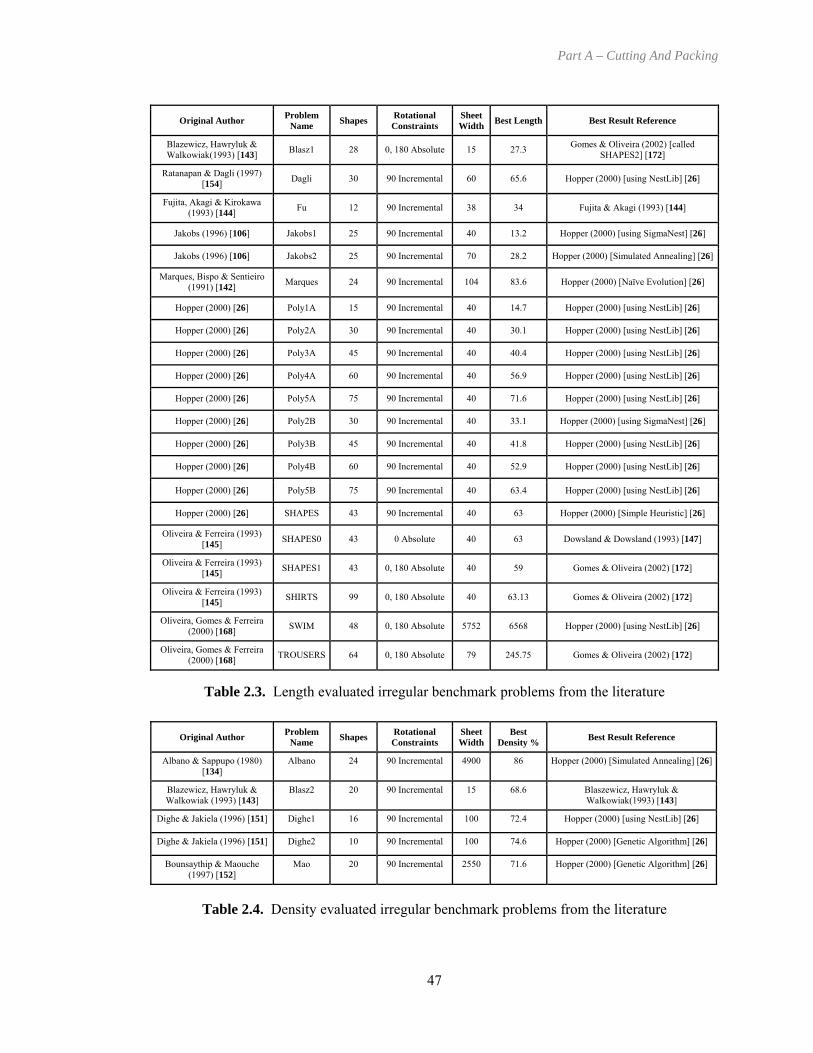
Part A – Cutting And Packing
Original Author Problem Name Shapes Rotational
Constraints Sheet Width Best Length Best Result Reference
Blazewicz, Hawryluk & Walkowiak(1993) [143] Blasz1 28 0, 180 Absolute 15 27.3 Gomes & Oliveira (2002) [called
SHAPES2] [172]
Ratanapan & Dagli (1997) [154] Dagli 30 90 Incremental 60 65.6 Hopper (2000) [using NestLib] [26]
Fujita, Akagi & Kirokawa (1993) [144] Fu 12 90 Incremental 38 34 Fujita & Akagi (1993) [144]
Jakobs (1996) [106] Jakobs1 25 90 Incremental 40 13.2 Hopper (2000) [using SigmaNest] [26]
Jakobs (1996) [106] Jakobs2 25 90 Incremental 70 28.2 Hopper (2000) [Simulated Annealing] [26]
Marques, Bispo & Sentieiro (1991) [142] Marques 24 90 Incremental 104 83.6 Hopper (2000) [Naïve Evolution] [26]
Hopper (2000) [26] Poly1A 15 90 Incremental 40 14.7 Hopper (2000) [using NestLib] [26]
Hopper (2000) [26] Poly2A 30 90 Incremental 40 30.1 Hopper (2000) [using NestLib] [26]
Hopper (2000) [26] Poly3A 45 90 Incremental 40 40.4 Hopper (2000) [using NestLib] [26]
Hopper (2000) [26] Poly4A 60 90 Incremental 40 56.9 Hopper (2000) [using NestLib] [26]
Hopper (2000) [26] Poly5A 75 90 Incremental 40 71.6 Hopper (2000) [using NestLib] [26]
Hopper (2000) [26] Poly2B 30 90 Incremental 40 33.1 Hopper (2000) [using SigmaNest] [26]
Hopper (2000) [26] Poly3B 45 90 Incremental 40 41.8 Hopper (2000) [using NestLib] [26]
Hopper (2000) [26] Poly4B 60 90 Incremental 40 52.9 Hopper (2000) [using NestLib] [26]
Hopper (2000) [26] Poly5B 75 90 Incremental 40 63.4 Hopper (2000) [using NestLib] [26]
Hopper (2000) [26] SHAPES 43 90 Incremental 40 63 Hopper (2000) [Simple Heuristic] [26]
Oliveira & Ferreira (1993) [145] SHAPES0 43 0 Absolute 40 63 Dowsland & Dowsland (1993) [147]
Oliveira & Ferreira (1993) [145] SHAPES1 43 0, 180 Absolute 40 59 Gomes & Oliveira (2002) [172]
Oliveira & Ferreira (1993) [145] SHIRTS 99 0, 180 Absolute 40 63.13 Gomes & Oliveira (2002) [172]
Oliveira, Gomes & Ferreira (2000) [168] SWIM 48 0, 180 Absolute 5752 6568 Hopper (2000) [using NestLib] [26]
Oliveira, Gomes & Ferreira (2000) [168] TROUSERS 64 0, 180 Absolute 79 245.75 Gomes & Oliveira (2002) [172]
Table 2.3. Length evaluated irregular benchmark problems from the literature
Original Author Problem
Name Shapes Rotational Constraints
Sheet Width
Best Density % Best Result Reference
Albano & Sappupo (1980) [134]
Albano 24 90 Incremental 4900 86 Hopper (2000) [Simulated Annealing] [26]
Blazewicz, Hawryluk & Walkowiak (1993) [143]
Blasz2 20 90 Incremental 15 68.6 Blaszewicz, Hawryluk & Walkowiak(1993) [143]
Dighe & Jakiela (1996) [151] Dighe1 16 90 Incremental 100 72.4 Hopper (2000) [using NestLib] [26]
Dighe & Jakiela (1996) [151] Dighe2 10 90 Incremental 100 74.6 Hopper (2000) [Genetic Algorithm] [26]
Bounsaythip & Maouche (1997) [152]
Mao 20 90 Incremental 2550 71.6 Hopper (2000) [Genetic Algorithm] [26]
Table 2.4. Density evaluated irregular benchmark problems from the literature
47

Part A – Cutting And Packing
2.6 Optimisation and Search Methods
This section details some of the search methods that have been used for automated packing
approaches. The seminal literature for each search method is provided where known and some
examples of where they have been applied to stock cutting problems are given.
2.6.1 Iterative Improvement Searches
The first class of searches involve so-called “iterative improvement searches” whereby the next
solution to evaluate belongs to the neighbourhood of the current solution. Such searches require
the definition of a suitable neighbourhood function to obtain a neighbouring solution. In terms
of rectangle packing, it is common to use a placement heuristic that places rectangles onto the
sheet in a given sequence. The sequence of rectangle identification numbers can be used to
generate a neighbouring solution, for example, by swapping two of the elements of the sequence
such as:
1,2,3,4,5,6,7,8 1,6,3,4,5,2,7,8
In this example, rectangles 2 and 6 have been swapped to produce a neighbouring solution
which can then be evaluated. After evaluating the sequence (by packing the rectangles using a
placement heuristic and examining the height and/or density), an action must be taken based on
the knowledge that is drawn from the evaluation. The nature of this action depends on the
specific search that is undertaken.
A further point of note is that all searches require an initial solution to be generated. Generally,
this is achieved by applying a constructive (normally quick) heuristic. In the case of the work
within this thesis, the initial solution is always based on the sequence produced by sorting the
shapes by decreasing height, width or area. This offers a reasonably good solution because the
48

Part A – Cutting And Packing
larger shapes are placed first and the smaller shapes can be placed in the holes between the
larger shapes or at the end of the layout. If the sequence was generated in the reverse, then the
larger shapes would all be placed at the end of the layout which would adversely affect the
solution quality.
2.6.1.1 Hill Climbing
The hill climbing algorithm (also known as the “gradient descent algorithm” when an evaluation
function is to be minimised) probably offers one of the simplest strategies for optimisation
problems. It involves maintaining one current solution and generating one neighbouring
solution, which is then evaluated. If the neighbour evaluates to a better quality solution than the
current solution, the current solution is replaced by the neighbour and the search continues by
generating a neighbour solution of the new current solution. If the neighbour is of worse quality
than the current solution, it is discarded and the process continues with the original solution. At
the end of the search, the best solution seen is returned (this will always be the current solution
in the case of hill climbing).
The main drawback of hill climbing is that it can pursue areas of the search space that result in
only a local optimum being found and because there is no means of backtracking or acceptance
of worse solutions. One proposed solution to avoid this problem is to randomly restart the
search if there has not been an improvement in solution quality for a specified number of
iterations.
Multi-neighbourhood hill climbing techniques have been utilised within chapter seven and
chapter nine of this thesis.
49

Part A – Cutting And Packing
2.6.1.2 Tabu Search
The tabu search algorithm extends the idea behind hill climbing and was first proposed in
Glover (1977) [177] but was not widely known and adopted until after Glover (1989) [178,179].
Unlike hill climbing, tabu search evaluates a subset of neighbouring solutions at each iteration
of the search and moves to the solution with the best evaluation value. The current solution is
always replaced with the best neighbour even if the new solution has a worse quality evaluation.
In addition to this, the approach also maintains a bounded list that contains a history of
previously seen solutions. This “tabu” list is used to avoid revisiting areas that have already
been examined in the recent history of the search. If this was not employed with a full
neighbourhood search, the search could potentially get stuck by alternating between the two
solutions (or a cycle of more than two moves) with the locally best quality evaluations. The
tabu list is not so important when only evaluating a subset of the neighbourhood as long as the
neighbouring solutions are chosen randomly.
Tabu search is used within chapters three, four, seven and nine of this thesis. Other examples
can be drawn from the following cutting and packing literature: [143,166,167,176,180].
2.6.1.3 Simulated Annealing
Simulated annealing originates from an algorithm presented by Metropolis et al. for the
simulation of the annealing of solids (Metropolis et al., 1953) [181] although the first application
of simulated annealing to searching within combinatorial optimisation problems was proposed
by (Kirkpatrick, Gelatt and Vecchi, 1983) [182]. The algorithm behaves the same as hill
climbing in accepting the neighbour solution when it is better than the current solution (i.e. the
neighbour replaces the current solution). However, one of the main features behind simulated
annealing is that it is able to accept worse solutions based on a probability function consisting of
two parameters: i) the difference in the evaluation quality of the current and neighbour solutions
50

Part A – Cutting And Packing
(known as the change in energy, ∆E), and ii) the duration of the search (known as the
temperature, T). The standard formula to calculate the probability of a worse solution being
accepted is e(-∆E/T). The temperature parameter is directly controlled by the cooling schedule
which is usually a linear or geometric scale that is applied to reduce the temperature after each
or a certain number of iterations.
It can be seen that as the temperature decreases or the neighbour solution becomes increasingly
worse than the current solution, there is less probability of accepting the neighbour solution.
Therefore, at the outset of the search there is a less stringent acceptance criterion and the
probability of accepting worse solutions is high whereas, as the search progresses and the
temperature is cooled, there is less probability of accepting a solution. When the temperature
becomes zero, the algorithm becomes the equivalent of hill climbing.
Simulated annealing is used in chapters three, four and five of this thesis but has also been
applied to packing problems in [116,117,118,120,142,183,184,185,186,187,188,189,190].
2.6.2 Genetic and Evolutionary Algorithms
Genetic algorithms are population based search methods inspired by the principal of evolution
found within the natural world. Although genetic algorithms were first conceived by Fraser in
1957 [191] and Bremermann in 1958 [192], Holland’s book of 1975 [193] is recognised as an
important work on the subject. A genetic algorithm maintains several solutions which are
known as individuals (or chromosomes). Each individual is composed of several separate parts
which are called genes. The actual values that are assigned to genes are called alleles. The
individuals of a population represent different solutions and, thus, it is important to evaluate the
quality of each individual. The numerical evaluation of an individual is known as its fitness.
51

Part A – Cutting And Packing
Throughout the course of the genetic algorithm, the population is constantly being replaced by
new individuals (i.e. new populations). This is achieved by applying two types of operator that
mimic the evolution of natural systems. The first operator is known as crossover and can be
thought of as the process of breeding. In the genetic algorithm, this is achieved by taking two
individuals, known as the parents, and recombining genetic material from within their genes in
order to produce new individuals or children. An important aspect of the algorithm is that
parents are selected in proportion of their fitness. This means that the fitter members of the
population are selected to breed more often than less fit individuals. Hopefully, the good
properties from a chromosome are propagated into new individuals and the population should
steadily improve as individuals become increasingly better. The second operator that is
commonly used is mutation. This aims to introduce diversity and allows for new genetic
material to be injected into the population. Usually, this takes the form of random value changes
to genes with a low probability. Genetic algorithms require specification of the following
operators and parameters:
Population Size: the number of individuals within the population
Measure of Fitness: the method used to determine the quality of individuals
Crossover Operators: how two chromosomes will be combined to produce children
Crossover Probability: individuals breed with some probability
Mutation Operators: how to mutate values within chromosomes
Mutation Probability: mutation is carried out with some (usually small) probability
Elitism: the best m individuals are carried forward into the next generation
A detailed analysis of genetic algorithms is provided by Goldberg [194]. A bottom-left-fill
hybridised genetic approach is examined as part of chapter three of this thesis but other
examples of genetic algorithms used for packing problems are found in the following:
[106,108,109,118,121,123,125,128,144,151,157,170,171,195,196,197,198,199,200,201,202,203
204,205,206]
52

Part A – Cutting And Packing
2.6.3 Other Search Methods
Two other optimisation techniques that have been applied to packing problems are: i) artificial
neural networks and ii) ant algorithms. Although these are not investigated within this work,
they are included here for completeness.
i) Artificial Neural Networks
Artificial neural networks are based on the modelling of information processing that occurs in
the brain. The system is made up of many simple nodes or neurons. Each neuron receives one
or more weighted inputs and then outputs some value depending on whether the total has
exceeded an activation level threshold value. A neuron is said to have ‘fired’ when it outputs a
value. Inputs can be excitatory or inhibitory. Excitatory inputs contribute positively to a
neuron’s total and inhibitory inputs contribute negatively. The outputs from neurons are inputs
to other neurons and, hence, complex networks can be created. Some neurons receive external
inputs which propogate through the neural network, inducing some to fire and others not to fire.
The network as a whole exhibits some behaviour through output nodes. The seminal study of
neural networks was conducted in 1943 by McCulloch and Pitts [207]. Within the domain of
cutting and packing, neural networks are generally combined with other search techniques and
can be used to produce input sequences to dictate the order in which shapes are to be packed.
They have also been used to create placement strategies for use in automated packing [26].
Examples of neural networks can be found in the following literature within the cutting and
packing field: [128,186,208,209].
ii) Ant Algorithms
The ant algorithm is a relatively new search methodology based on the observation that ants can
find the shortest route between their habitat and a food source, even though they are almost
53

Part A – Cutting And Packing
completely blind. Ant algorithms (also known as ant systems) are also population based
strategies with each ant representing one potential solution. The ants ‘communicate’ by
depositing of pheromone trails. An example of the ant algorithm in operation can be drawn
from a simple problem, discussed in the seminal work by Dorigo in 1996, involving a problem
whereby ants must travel between two locations (i.e. a nest and a food source) [210]. In the
simplest case, the ants only need to travel in a straight line. However, if an object is blocking
the path of the ants then the ants must decide whether to move left or right around the object.
Assume that the path to the right is shorter than the left path. Also assume that ants deposit
pheromone trails as they move and that ants prefer to follow paths which have been taken by
other ants. When the first ant reaches the object, there will be no pheromone trail to guide the
ant’s decision. Therefore a random choice will be made. When subsequent ants reach the object
they will either go left or right around the object (laying pheromone trails as they move). Now
the first ant returns from the food source and reaches the object once more. This time there will
be higher levels of pheromone on the shorter path as more ants have reached the end of this path
(because the ants have travelled less distance than ants taking the other path) and, therefore, the
ants returning from the food source are under greater influence to take this path as it has a
stronger pheromone trail. The system works with positive feedback whereby the greater the
number of ants that follow a particular path, the larger the pheromone trail becomes on that path
and the more desirable it becomes for future ants.
Ant algorithms have been used in the following packing approaches within the following
literature: [7,9,211,212].
2.7
54

Part A – Cutting And Packing
Packing within Industry
Packing problems occur in many important mass-production industries. Within this section,
these industries are identified and the related academic literature that has specifically attempted
problems arising from the industrial setting are discussed.
2.7.1 Identification of Applicable Industries
2.7.1.1 Paper
The first work into cutting and packing was conducted in the 1950-1960s and addressed
problems from within the paper industry. This initial research was conducted to find the optimal
way that a roll of paper may be cut into desired pieces and used linear programming techniques
on a restricted guillotine variant of the orthogonal packing problem [213,214]. More recent
examples of research that has been based on the paper industry are presented by Johnson,
Rennick and Zak (1997) who extend the one-dimensional stock cutting problem to include the
process of “skiving” (joining of lengths of paper) [215]. The authors stated that, through the
skiving process, solutions can be found for instances that could not be solved previously. A
heuristic and exact method is described that can produce a solution to a 30 roll problem within
around one minute of computation time. Harjunkoski, Westerlund, Porn and Skrifvars (1998)
presented two integer programming algorithms for cutting larger stock rolls of paper into
product paper rolls and compare them using a real-world instance from a Finnish paper
converting mill [216]. Aboudi and Barcia (1998) used linear programming methods for the
paper cutting industry but also deal with defective areas that can appear through manufacturing
glitches [217]. A defective area cannot be used when cutting out product rolls. Defective sheets
were first investigated by Hahn in 1968. Hahn produced an optimal algorithm based on Gilmore
and Gomory (1966) [74] for cutting out multiple identical sheets containing rectangularly
55

Part A – Cutting And Packing
defined defective areas [218]. An important feature of the algorithm was that larger rectangles
were placed first because the sheets had more restricted potential positions because of the
defects. McDiamid (1999) presented heuristic methods for a very restricted case of the stock
cutting problem [219]. Once more, jumbo reels (or “raws”) must be cut into smaller product
reels (or “finals”) but it is known that it is only ever possible to cut two product reels out of each
jumbo (never three or more). McDiamid stated that even this problem is strongly NP-hard.
Menon and Schrage (2002) provided an integer programming approach to solve instances of the
problem involving the order allocation problem on multiple parallel cutting machines [220].
Their approach produced solutions in 10.12, 37.04 and 118.39 seconds, respectively, for two,
three and four parallel machine problems. Multiple parallel machines are the focus of Giannelos
and Georgiadis (2001) who also used exact techniques [221].
2.7.1.2 Wood
The wood cutting industry has also been the subject of stock cutting research. Morabito and
Garcia (1998) tackled a similar problem to the paper industry except that sheets of hardboard are
dissected into smaller rectangular by circular saws (and thus the problem is guillotine as the
blades may not turn mid-cut) [222]. They compared two techniques to solve problem instances
that are taken from the Brazilian hardboard industry. The first is a dynamic programming based
integer program and the second is a simple extension of the algorithm presented in Gilmore and
Gomory (1963) [72]. The flat-pack furniture producing industry is the subject of Morabito and
Arenales (2000) [223]. The authors draw particular attention to the balance between producing
less wastage and producing more simple layouts that can be cut with less complication. The unit
cost of material is factored into the algorithms such that, for cheap material, the layout becomes
secondary to the simplicity of the cutting process. However as unit cost rises, there becomes
more emphasis on the reduction of waste (at the expense of cutting difficulty).
56

Part A – Cutting And Packing
2.7.1.3 Glass
Glass cutting almost always involves the rectangular guillotine variant of the stock cutting
problem. This is because the glass must firstly be ‘scored’ and then snapped over a flat edge.
Bisotto, Corno, Prinetto, Rebaudengo and Reorda (1997) [224] hybridise a greedy placement
heuristic with a genetic algorithm in order to solve the trim loss glass production problem. The
purpose of the genetic algorithm is to generate orderings of the rectangles which are then
decoded into different layouts by the placement heuristic. The approach compares favourably
against other approaches and has now been adopted by one manufacturer of glass cutters.
Puchinger, Raidl and Koller (2004) [225] developed evolutionary algorithms to solve glass
cutting problems from the real world. They compared a greedy first-fit heuristic, two branch-
and-bound tree search procedures and different variants of an evolutionary approach. They
suggested that the evolutionary algorithms perform well in practice although they are
occasionally outperformed by the other methods.
2.7.1.4 Textiles
The textiles industry also provides a test bed in which to apply automated packing research. The
cutting of clothes from material rolls offers many difficulties and nuances that must be handled
by any automated approach. Such problems may include patterned rolls of materials and, hence,
rotational constraints on the orientations in which clothing can be cut (when pieces are stitched
together, patterns must be aligned). Further to this, highly irregular shapes are usually involved,
requiring complex geometric handling, and defective areas may be present within the material
rolls (which, in general, must be identified by human operators). Although the general irregular
problem has its foundations with Adamowicz and Albano (1976) [85], there has not been
substantial research interest in the textile problem until the last ten years. This could potentially
be explained by complex modelling that is required by the high irregularities within shapes and
sheets. However, there are now many instances of literature on this problem due to additional
57

Part A – Cutting And Packing
cooperation and funding from within the textile industry. Chryssolouris, Papakostas and
Mourtzis (2000) tackled the scheduling of nesting operations that takes into account both nesting
efficiency and further production objectives such as meeting due dates, minimising cost,
maximising machine throughput and maximising material utilisation [226]. They produce a
scheduling approach and then use rule based transformations to also produce nesting solutions
for the rectangular version of the problem. The work was conducted with a carpet weaving firm.
In 2002, Degraeve, Gochet and Jans extended the work presented by Degraeve and Bandebreok
(1998) [227] using mixed integer programming methods for solving marker layout problems in
the fashion industry. They factor ‘bill of material’ requirements (the demand and requirement of
individual pieces to fulfil an order) into the objective and evaluation criteria. The authors then
further extended the model to include different colours of materials [228]. Yeung and Tang
(2003) approach the strip packing problem for the cutting of larger rolls of material into smaller
rectangular pieces within Hong Kong’s clothing industry (note the similarity to the paper
industry above) [201]. They utilised a genetic algorithm based approach to generate
permutations for the so-called lowest-fit-left-aligned decoder heuristic (although this is similar
to the bottom-left class of heuristics, they use a similar representation of the height ‘skyline’ of a
partial layout as is presented for the best-fit heuristic in chapter three).
2.7.1.5 Leather and Footwear
The leather cutting industry has also been the focus of some of the latest work into cutting and
packing. Crispin, Clay, Taylor, Bayes and Reedman, in 2003, addressed the problem of leather-
lay planning for the footwear industry [200]. Leather ‘hides’ have considerable variability in: i)
the strength of the leather, ii) direction of this strength and iii) regions of differing quality.
These factors often severely restrict potential placements of shapes and the variability in hides
generally requires human operator input to either oversee the entire process or to define the
areas of strength (unless X-ray techniques are used). The authors use an imaging technique to
58

Part A – Cutting And Packing
generate no-fit polygons of the sheet and the shapes and then use genetic algorithms to generate
shape angles and nesting direction. This is complicated by almost free rotation being allowed
(shape angles are mutated in 5° increments) and many no-fit polygon generations must be made
on-line. The algorithm cannot perform within the same timeframes as skilled experts. Other
approaches that focus on leather lay-planning can be found in Bounsaythip, Maouche and Neus
(1995) [229] where the authors approached the layout problem by using evolutionary search
techniques and in Heistermann and Lengauer (1995) [230] who highlighted some of the
problems that are found within the industry.
2.7.1.6 Plastics and Foam
Whilst the author has been unable to establish academic literature that specifically addresses the
plastic cutting industry, the problem does not differ from those found in the other industries and,
therefore, the majority of techniques from other methods can be applied. The problem usually
includes the multisheet two-dimensional irregular variant but shapes are generally convex. This
information was gathered during this research programme through correspondence and visits to
Ultraframe Limited, a UK conservatory manufacturer who are required to cut roofing panels
from polycarbonate sheets.
2.7.1.7 Metals
Metal cutting is of interest because of the wide range of operational considerations that may
occur. For example, the material costs can vary considerably, from thin aluminium to processed
metals that can have thicknesses of several centimetres (or even metres in the case of power
station reactor linings). This generally has an impact on the amount of computation time that
one would be willing to allow an automated strategy. In the aluminium case the importance of
generating the optimal layout is probably secondary to producing a quick solution as minimal
cost savings can be achieved and it is important to keep the production line operating. However,
59

Part A – Cutting And Packing
thick processed metals have high unit cost and every improvement in material utilisation can
yield significant cost savings. Nonås and Thorstenson (2000) [231] attempted a stock cutting
problem from a Norwegian off-road truck production company whereby the majority of the
parts required for production of the trucks are made in-house. The authors presented three local
searches and column generation approaches but restrict the problem such that only sheets with
common dimensions are used. In 2002, Kos and Duhovnik used the steel structure production
industry where cutting beams into smaller pieces is of importance [232]. They showed that a
genetic algorithm with domain specific information and a local search can achieve
improvements of around 5% over initial solutions. Further examples can be drawn from the
literature that was discussed in section 2.3.
2.7.2 Cutting Technologies and their Implications
The purpose of this section is to highlight some of the real world difficulties that occur from the
use of different types of cutting technology. This information is reported to show the complex
nature of industrial problems and was gathered from discussions with our industrial partner.
2.7.2.1 Stamping
Stamping is mainly used to cut multiple identical shapes out of a sheet of material (mainly
metals) as different shapes require costly production stoppages to change the cutting plate. The
process involves applying a large downward force onto the sheet by a heavy block of metal with
a cut plate attached to its face.
2.7.2.2 Knife Cutting
Knife cutting offers its own challenges because the blade has limited freedom once a cut is
started (i.e. it cannot make lateral movements). Therefore, when cutting shape corners, the
blade must be removed, rotated and then pierced back into the material. Another complication
60
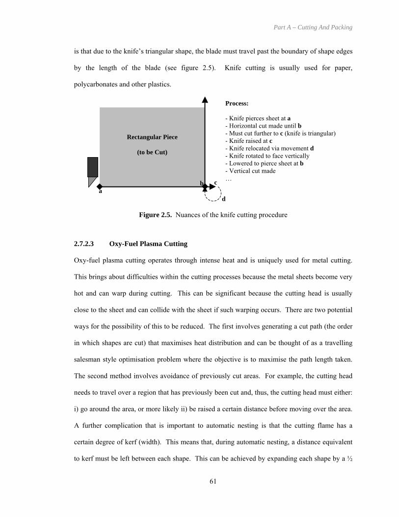
Part A – Cutting And Packing
is that due to the knife’s triangular shape, the blade must travel past the boundary of shape edges
by the length of the blade (see figure 2.5). Knife cutting is usually used for paper,
polycarbonates and other plastics.
Rectangular Piece
(to be Cut)
d
Process: - Knife pierces sheet at a - Horizontal cut made until b - Must cut further to c (knife is triangular)- Knife raised at c - Knife relocated via movement d - Knife rotated to face vertically - Lowered to pierce sheet at b - Vertical cut made … c b
a
Figure 2.5. Nuances of the knife cutting procedure
2.7.2.3 Oxy-Fuel Plasma Cutting
Oxy-fuel plasma cutting operates through intense heat and is uniquely used for metal cutting.
This brings about difficulties within the cutting processes because the metal sheets become very
hot and can warp during cutting. This can be significant because the cutting head is usually
close to the sheet and can collide with the sheet if such warping occurs. There are two potential
ways for the possibility of this to be reduced. The first involves generating a cut path (the order
in which shapes are cut) that maximises heat distribution and can be thought of as a travelling
salesman style optimisation problem where the objective is to maximise the path length taken.
The second method involves avoidance of previously cut areas. For example, the cutting head
needs to travel over a region that has previously been cut and, thus, the cutting head must either:
i) go around the area, or more likely ii) be raised a certain distance before moving over the area.
A further complication that is important to automatic nesting is that the cutting flame has a
certain degree of kerf (width). This means that, during automatic nesting, a distance equivalent
to kerf must be left between each shape. This can be achieved by expanding each shape by a ½
61

Part A – Cutting And Packing
kerf before automatic nesting commences. This expansion operation generally introduces arcs
into shapes where none existed before (see figure 2.6).
Figure 2.6. Expanding shapes by ½ kerf width
Further problems can occur from ‘burring’ when travelling around corners. This is mainly due
to the cutting flame being in contact with a singular point for longer duration and causing u
½ Kerf
½ Kerf
ntidy
dges. Referring to figure 2.6, when the cutting flame cuts around the triangle corners, it is in
whole time and the continuous high temperatures can result
be used on any material. It benefits
e s of oxy-fuel plasma cutting are avoided,
purposes of automatic nesting within the industrial setting.
e
contact with the triangle vertices the
in less defined corners due to heat damage. A solution to this is to perform what are known as
“butterfly cuts” which perform a similar cutting path to the knife cutting example of figure 2.5.
This ensures that crisp edges are cut but it requires the use of additional parts of the sheet.
2.7.2.4 Water-jet Cutting
Water-jet cutting involves the high-powered streaming of water reinforced with sand grits. This
cutting technology is the most flexible and can, generally,
from b ing a cool cutting method, and so the problem
but it still has a certain amount of kerf. Also as the cutter moves, the angle of the jet will alter in
proportion to its speed. These are all practical factors that must be dealt with during cutting but
it is only really kerf width (and hence, arcs) that needs to be handled appropriately for the
62

Part A – Cutting And Packing
2.7.3 Additional Objectives and Considerations
Automatic nesting software within the industrial setting may be required to cope with other
bjectives (apart from utilisation). Whilst these considerations do not feature in this work, they
problems that appear within the industrial domain and,
me cutting technologies can have multiple cutting heads to reduce the throughput time of
cutting heads move using the same CNC cutting machine
.7.3.2 Multiple Sheets
erent-dimensioned sheets also add extra complication as
of
the sheet through CAD definitions, then the process can be slow. Previously, industry has taken
straight line offcuts of the sheet to avoid this problem (by creating another rectangular sheet). If
o
do provide an interesting insight into
therefore, some of these are briefly described below and have been discovered from time spent
with the industrial partner.
2.7.3.1 Multi-head Cutting
So
cutting operations. Generally, the
controller code and therefore make identical cuts (at an offset). In order to utilise such facilities,
nesting algorithms should place multiple shapes copies within the correct offset bounds.
2
The inclusion of multiple diff
algorithms must ‘decide’ which sheet sizes to employ for particular jobs. The correct selection
of sheets can drastically reduce trim-loss and restocking costs.
2.7.3.3 Partial Sheet Usage
One important aspect of increased profitability is the reutilisation of partly used sheets. Any
areas of the sheet which have not been used can be restocked and presented in future jobs.
However, if the task of reintroducing the sheet to nesting is performed through manual input
nesting operations can effectively store offcuts (as a post process) into a database of available
sheets, the entire offcut can be reused (even with considerable irregularities and holes).
63

Part A – Cutting And Packing
2.8 Cutting and Packing: Summary
interrelated problems that exist within the research area were described. The typological
In this chapter, an overview of the field of cutting and packing was provided and some of the
categorisation of problems was discussed, indicating the deficiencies in the current system
(presented by Dyckhoff in [20]), and reported on the concerted efforts to produce a better
typological categorisation model within the academic community. Further to this, 42 survey
and packing.
the remainder of this thesis, namely non-guillotine two-dimensional rectangular packing and
irregular packing. These reviews included the publications that the author of this thesis has
ost useful for the work presented in this thesis. Both reviews concluded with a
summary of the readily available benchmark datasets and their sources from within the
literature.
processes are an important consideration. Further to this, a summary of published work that has
addressed problems from each of the identified industries was given. The implications that
problem have also been discussed. Finally, additional considerations that are related to
production management within the industrial setting were highlighted. A large proportion of
this information was obtained through discussions with the industrial partner and is, therefore,
biased towards the metal cutting industry. However, many of the issues found in metal cutting
processes can be directly related to problems within other industries.
papers were identified that provide good overviews and bibliographies for the field of cutting
After this, two literature reviews were provided for the packing problems that are the focus of
found the m
The chapter concluded by identifying the different industries for which cutting and packing
cutting technology has on the process of automatic packing for real world applications of the
64

Part B – Rectangular Packing
PART B – RECTANGULAR PACKING
The two-dimensional orthogonal stock cutting problem consists of the assignment or placement
of rectangular pieces onto a larger rectangular sheet of material such that pieces do not overlap
and the total height required is minimised. This problem has been shown to be NP-hard and,
therefore, it is strongly believed that it cannot be solved within polynomial time (Garey and
Johnson, 1978) [15]. The problem exists in two variants, guillotine and non-guillotine, which
mainly depends on the cutting technology being employed. The key feature of the guillotine
variant is that pieces must be assigned to the sheet so that they may be cut out from the sheet by
successive guillotine cuts that span the entire width or length of the sheet. The non-guillotine
variant does not have this constraint but does require a cutting technology that can either change
direction whilst cutting or one that can pierce the middle of a sheet. These are practical issues
that are important when a particular layout will be physically cut from a sheet of material.
The work presented in this section of the thesis specifically addresses the non-guillotine variant
of the problem in which we are not restricted to only performing full horizontal or vertical cuts
from one sheet edge to another (unlike guillotine packing). All items in the set of rectangles
must be packed onto the object sheet and pieces can undergo rotations of 90° to allow rectangles
to be placed in either their portrait or landscape orientations. The author has evaluated the
presented approaches on a wide range of benchmark data involving 34 problem instances from
various sources within the literature and, further to this, has generated and presented 28 new
rectangular benchmark problem instances to the academic community to aid comparison
65

Part B – Rectangular Packing
between previous approaches and the new methods presented in this thesis. The author also
hopes that this will help to facilitate further research within the field of cutting and packing.
The first chapter in this section, chapter three, introduces an extremely fast heuristic placement
approach that is based on the principals of best-fit. The heuristic yields significant
improvements over the previous state-of-the-art approaches from within the literature when
applied to readily available benchmark problems (of which the author of this thesis is aware
from previously published datasets) that have been provided by other researchers within the
field. Specifically, the quality of solutions generated with the best-fit heuristic can be within 2%
of the optimal solutions and, furthermore, are produced within a few seconds. Two
implementations are provided to cope with integer and floating point data respectively. This was
the first significant contribution that the author has brought to the field of cutting and packing
during the course of the research programme and was published in the following publication:
Burke, E. K., Kendall, G., Whitwell, G., 2004, “A New Placement Heuristic
for the Orthogonal Stock Cutting Problem”, Operations Research, Vol. 52,
No. 4, July-August 2004, pp. 655-671. [1]
Chapter four presents a new hybrid approach that combines the respective strengths of the best-
fit heuristic (from chapter three) and state-of-the-art metaheuristic bottom-left-fill approaches
that had previously produced the best quality solutions to benchmark datasets. The main
principle of the approach is that the best-fit heuristic produces the initial layout and then the
metaheuristic approach is applied to the last m rectangles to evaluate different rectangle
arrangements. Once again, experimentation is performed on the benchmark problem instances
to i) identify the optimal value for m, ii) compare against the best-fit heuristic and the
metaheuristic bottom-left-fill methods alone, and iii) investigate the impact of longer run times.
Further improvements in solution quality are achieved over best-fit and other previous
66

Part B – Rectangular Packing
approaches by using the presented hybrid approach. The hybrid approach appears in the
following contribution:
Burke, E. K., Kendall, G., Whitwell, G., 2005, “Metaheuristic Enhancements
of the Best-Fit Heuristic for the Orthogonal Stock Cutting Problem”,
INFORMS Journal on Computing (in review). [3]
The last chapter of this section, chapter five, investigates the advantages that can be achieved, in
terms of solution quality, through the utilisation of user interaction in order to ‘guide’ the
automation. This is achieved by revisiting the hybrid approach of chapter four except that it is
modified to allow user interaction through the selection of unsatisfactory regions within the
generated layouts (that is the rectangles are now selected by the user). A metaheuristic search
can then be invoked to specifically concentrate on the user-defined regions. This process can be
repeated until no more improvements in quality are achieved or until the user is satisfied with the
solution. One of the main principles of the approach is that the user retains control over the
automation process but is abstracted away from directly moving individual rectangles. Once
again, large improvements in solution quality are made over the previous techniques from the
literature (and methods from chapters four and five) against the benchmark problems. The
interactive approach presented within chapter five is the focus of the following paper:
Burke, E. K., Kendall, G., Whitwell, G., 2005, “The Two-Dimensional
Orthogonal Stock Cutting Problem: A New User-Guided Hybrid Approach”,
Journal of the ACM (in review). [5]
The data for the newly generated rectangular problem instances that are used within this thesis
are provided in appendix C and the solutions produced for the entire set of rectangle benchmark
problem instances are displayed in appendix A of the thesis.
67

Part B – Rectangular Packing
CHAPTER THREE
The Best-Fit Placement Heuristic
3.1 Overview
Unlike the bottom-left and bottom-left-fill methods (described in section 2.2.1) that make
placements which are based on the sequence of rectangles supplied to them, the proposed
heuristic method dynamically selects the next rectangle for placement during the packing stage.
This enables the algorithm to make informed decisions about which rectangle should be packed
next and where it should be placed. A best-fit type strategy is adopted for this purpose. This is,
essentially, a greedy algorithm that attempts to produce good quality packings by examining the
available space within the stock sheet and then placing the rectangle that best fits the lowest
space available. There are some inherent problems with respect to the time complexity of the
algorithm and the quality of the solution. In order to find the lowest available gap, the stock
sheet and current assignment of shapes must be examined. Once the lowest gap is found, the list
of rectangles must be searched in order to find the best fitting shape. Both of these operations
must be conducted at each step of the algorithm and therefore they contribute towards increasing
the time complexity. In section 3.2.1, methods are addressed that can be employed to reduce
this complexity bottleneck.
At the beginning of the packing process there will not be any shapes assigned to locations on the
stock sheet. Therefore, the lowest available gap or ‘niche’ for placement of a shape will be the
entire width of the stock sheet. As shapes are placed, the lowest gap will change with respect to
both location and width. The best fitting shape is always selected and placed within this gap.
68

Part B – Rectangular Packing
There are three possibilities: i) there is a shape with a dimension (either width or height) that
exactly fits the gap, ii) there is a shape with a dimension smaller than the gap, or iii) there are no
shapes that will fit the gap. In the first case, the rectangle placement is easy because there is a
perfect fit (where there are several shapes that would fit exactly, the rectangle with the largest
area is chosen). However, in the second case the shape that consumes the largest portion of the
gap is placed. As this shape does not completely fill the gap, it needs to be defined how a shape
should be placed within the gap. This has been termed the niche placement policy. The third
case gives rise to an important property of using the best-fit methodology. If none of the
available rectangles can fit within the lowest gap then the relevant space can be considered
wastage. This is clear because if none of the shapes fit the space now then none of the
remaining shapes will be able to fit in the space in future iterations because new rectangles are
never added to the list of shapes to be placed. Therefore, unlike the bottom-left placement
heuristic, this method only ever creates holes that cannot be filled and unlike bottom-left-fill, all
holes that are created can be ‘forgotten’. This leads to another important feature of the best-fit
heuristic. Many algorithms, such as bottom-left and bottom-left-fill, require a costly ‘overlap’
function. This performs an overlap test between the current shape and each of the shapes that
have previously been placed onto the sheet. Obviously the more rectangles that have been
packed, the more overlap tests have to be performed thus resulting in the process becoming
increasingly slower as each rectangle is placed. However, because of the best-fit approach and
the implementation (presented in section 3.2), this operation is not required as it is always the
case that the shapes being placed do not overlap with other rectangles.
3.1.1 Niche Placement Policies
The best-fit heuristic is a combination of three niche placement policies with each policy
indicating how a shape could be placed when it does not exactly fit the lowest niche. The
heuristic never deliberately creates a niche but, if no rectangle can fit the gap completely, there
69

Part B – Rectangular Packing
is no option but to create one. In the following niche placement policies, it is assumed that the
stock sheet sides are ‘infinitely tall’ to simulate a roll of material.
Place at Leftmost
The leftmost niche placement policy places a non-exact fitting rectangle at the left side of the
niche. Note: if a rightmost niche placement policy were used, the resultant packing would be a
mirror image of the leftmost policy.
Place Next to Tallest Neighbour
In this placement policy the two rectangles on the stock sheet that define the lowest gap are
examined. The best fitting rectangle is then placed within the gap next to the tallest gap-
defining rectangle (see figure 3.1). If the lowest gap is defined by a rectangle and the sheet side,
then the rectangle is placed next to the sheet side.
Lowest Tallest Neighbour
Best Shortest Neighbour
Figure 3.1. Placement next to tallest neighbour
Place Next to Shortest Neighbour
This placement policy is the opposite of the tallest neighbour policy described above. This time,
rectangles are placed next to the shortest neighbour. An example is given in figure 3.2.
Figure 3.2. Placement next to shortest neighbour
Lowest Tallest Neighbour
Shortest Neighbour Best
70

Part B – Rectangular Packing
3.1.2 Improving the Packing
A drawback of using the proposed method is that it can create poorer quality packings due to
‘towers’. Towers are produced when long thin rectangles have not been placed until the latter
stages of the layout. The algorithm may place these rectangles in portrait orientation near to the
top of the layout where they can negatively affect the solution quality. Due to this problem, a
further step is conducted after all rectangles have been placed. This searches for the shape that
is currently adding the greatest height to the packing and determines if it is a tower by
examining if the rectangle’s height is greater than its width. If the rectangle is identified as a
tower, the rectangle is removed from the packing, is rotated by 90 degrees and then repacked in
e new orientation on top of the layout. If the solution quality is improved by this step then it
is repeated on a new ‘tower’. This process continues until there is no improvement in solution
ore detail in implementation section 3.2.3.
eet at every time step of the algorithm. These are
omputationally expensive operations and the algorithm would benefit if these could be
. The inputs to the algorithm are a list of rectangles in random
th
quality. The procedure is described in m
3.2 Implementation
The description of the algorithm above requires a search for both the best fitting rectangle and
the lowest space within the stock sh
c
simplified or, better still, removed
order and the width of the stock sheet.
3.2.1 Pre-Processing Stage
Firstly, the problem of representation is addressed. Some algorithms store this information
using location points as in the bottom-left-fill algorithms (Chazelle, 1983) [111] and/or collision
detection by the sliding of shapes such as the bottom-left algorithms (Jakobs, 1996 [106]; Liu
and Teng, 1999 [108]). Others avoid the problem by packing in rows with a new row starting
71

Part B – Rectangular Packing
from the highest point of the previous one (Bengtsson, 1982) [104]. However, these methods
require the maintenance of potential location lists that must be traversed and/or collision
detections on each rectangle placement. Collision detection is computationally expensive due to
the need to examine all of the already placed rectangles when adding a shape. Therefore when
adding the last piece in a problem of n shapes, n – 1 collision tests are required to ensure that
there are no overlaps with other placed shapes. In the case of Bengtsson’s row packing
approach, there is no overlap detection but there can be a significant increase in sheet wastage
between rows. The proposed approach eliminates the need for intersection testing by
representing the stock sheet as a linear array in which the number of elements is equal to the
width of the stock sheet. Whilst this is sufficient for integer data, floating point data must be
scaled and rounded to the desired accuracy for the representation (see section 3.2.4). Each
element of the array holds the total height of the packing at that x coordinate of the stock sheet.
can be thought of as maintaining the height profile or “skyline” of the layout.
Two xamples are given in figure 3.3 to show a sheet of 9 units width when empty and the same
sheet after packing seven rectangles.
he lowest space of the stock sheet can be found by locating the
775 4 0
Thus this array
e
Figure 3.3. Storing the skyline heights of the layout on a sheet of width 9 units when empty and
after packing seven rectangles
Therefore, the coordinate of t
smallest valued entry of the array. The width of the gap can be found by examining how many
consecutive array items of equal value exist. In figure 3.3, the lowest available space is located
at x = 0 and has a width of 3.
4 4 4 7 7 5 5 61 2 3 6 8Array Index
075 4 0
0 0 0 0 0 0 0 01 2 3 6 8
0 1
3 4
2
5 6
0 1 2
5 6
3 4
7 7
72

Part B – Rectangular Packing
The other problem encountered is caused by the best-fit methodology. The rectangle data is
defined as a list of rectangles each denoted by a (width, height) pair. In an unsorted list all n
rectangles must be examined to be sure that there is not a ‘better’ fitting rectangle available for
placement. However, the list of rectangles can be sorted once before packing commences so
that the nu erage per
rectangle placement). The first stage of this restructuring is to rotate any rectangle for which the
,5), (5,2), (1,1), (7,3), (1,2) } becomes { (5,3), (5,2), (1,1), (7,3), (2,1) }
Next, the rectangles are sorted into decreasing width order (resolving equal widths by decreasing
le 1. The search must continue because there may be a rectangle with a width of 4
mber of rectangles that need to be examined can be reduced to ½ n (on av
height is greater than the width. For example:
{ (3
height order):
{ (5,3), (5,2), (1,1), (7,3), (2,1) } becomes { (7,3), (5,3), (5,2), (2,1), (1,1) }
This list of rectangles can now be examined for the best fitting rectangle without the need to
search the entire list. For example, suppose we require a shape to fill a gap of 6 units. The first
rectangle in the list is examined, (7,3). Note that this rectangle could fill 3 units of the gap if
rotated. The second rectangle in the list, (5,3), can occupy a gap of 5 units. At this point the
search can be terminated, as all remaining rectangles have dimensions of equal or lower value
than 5. Assume that this time there is a gap of 4 units. The first rectangle in the list is
examined, (7,3). It can fill 3 units if rotated. The second rectangle is examined, (5,3).
Although it has an equal capacity as the first rectangle to fill 3 units of the gap, it is preferable to
pack larger rectangles first and so the search continues. The third rectangle, (5,2), is not better
than rectang
units. The fourth rectangle is examined, (2,1). Now the width of this rectangle is worse than the
current best so the search can terminate. The first rectangle would be returned as the best fitting
rectangle.
73

Part B – Rectangular Packing
Also note that as soon as a rectangle that fits exactly is found, it is selected. This reduces the
search time of the process and, due to the list structure, rectangles will have smaller dimensions
s the list is traversed. In general, it is better to place shapes with larger dimensions earlier in
he end of the packing where they may be allowed to protrude at the
the rectangle from the rectangle list and update
e stock sheet array. If the best fitting rectangle does not completely fill the gap, then there is
p
last shape placed left in gap then: New Gap Location = (Gap Location) + (Placed Rectangle Width)
l s p l d n p e New Gap Location = Gap Location
: New Gap Width = (Gap Width) – (Placed Rectangle Width)
a
the packing than towards t
top of the layout and affect solution quality.
3.2.2 Packing Stage
Firstly, the stock sheet is examined to find the lowest available gap (initially at x = 0, y = 0, and
lasting the entire sheet width). The rectangle list is examined and the best fitting rectangle
returned. This is placed within the gap depending on the current placement policy (as described
in section 2). The rectangle is assigned coordinates and removed from the rectangle list.
Finally, the relevant stock sheet array elements are incremented by the rectangle height. The
process continues: find the position of the lowest gap, find the width of the lowest gap, find the
best fitting rectangle, assign coordinates, remove
th
no need to locate the lowest gap for the next rectangle because it is a portion of the recent ga
and can be found by the following (figure 3.4):
If
If
The gap’s width is found by
ast ha e p ace right i ga th n:
4 4 4 0 0 0 0 6 6 4 4 4 2 2 0 0 6 6
Figure 3.4. Finding a new gap when the old gap has not been completely filled
Location = 3 Width = 4
New Location = Old Location + Rectangle Width = 3 + 2 = 5 New Width = Old Width – Rectangle Width = 4 – 2 = 2
74

Part B – Rectangular Packing
If a gap is found for which no remaining rectangle can fit, then this is wasted space and the stock
sheet array elements that reference the gap are raised up to the lowest neighbour. Assume there
a gap of 2 units but that there are no rectangles with a dimension of 2 units or less within the
rectangle list (figure 3.5).
ap is examined, a height of 2 to the left and 6 to the right. The array elements that define the
f the lowest neighbour element (in this case to a height of 2).
er
is
Figure 3.5. Procedure when no rectangle will fit gap
In figure 3.5 there is a gap for which no rectangle is small enough to fit. Each neighbour of the
g
gap are incremented to the height o
The array is now re-checked for the lowest gap and packing continues. In raising some of the
array elements it cannot be assumed that the new lowest gap is at a height of 2 because there
may be more gaps at a height of 0 or 1, so the array must be rechecked.
3.2.3 Post-Processing Stage
Once every rectangle is packed, all of the rectangles are examined to find if any are protruding
from the top of the packing and negatively affecting solution quality. When the highest
positioned rectangle is found, if the rectangle is orientated in such a way that its height is greater
than its width then it is removed from the packing and the stock sheet array is reduced by the
relevant rectangle height. Note that if the rectangle is found orientated with its width greater
than its height, then the height of the packing cannot be improved (reduced) as this rectangle is
in the lowest position possible. Then the rectangle is rotated so that its width has the larg
4 4 4 2 2 0 0 6 6 4 4 4 2 2 0 0 6 6
Waste
4 4 4 2 2 2 2 6 6
75
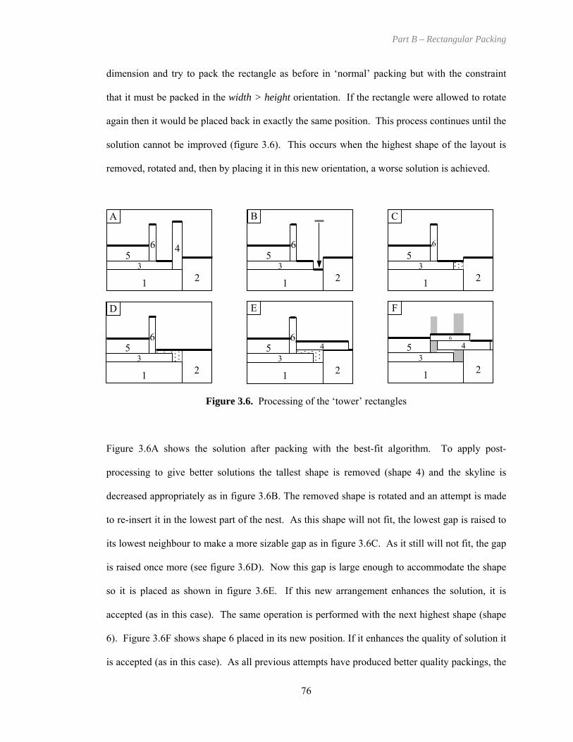
Part B – Rectangular Packing
dimension and try to pack the rectangle as before in ‘normal’ packing but with the constraint
ust be packed in the width > height orientation. If the rectangle were allowed to rotate
again then would be placed back in exactl e position. This process continues until the
solution cannot be improved (figure 3.6). This occurs when the highest shape of the layout is
removed, rotated and, then by placing it in this new orientation, a worse solution is achieved.
ccepted (as in this case). The same operation is performed with the next highest shape (shape
placed in its new position. If it enhances the quality of solution it
is accepted (as in this case). As all previous attempts have produced better quality packings, the
that it m
it y the sam
1 2 3
4 5
6
1 2
Figure 3.6. Processing of the ‘tower’ rectangles
Figure 3.6A shows the solution after packing with the best-fit algorithm. To apply post-
processing to give better solutions the tallest shape is removed (shape 4) and the skyline is
decreased appropriately as in figure 3.6B. The removed shape is rotated and an attempt is made
to re-insert it in the lowest part of the nest. As this shape will not fit, the lowest gap is raised to
its lowest neighbour to make a more sizable gap as in figure 3.6C. As it still will not fit, the gap
is raised once more (see figure 3.6D). Now this gap is large enough to accommodate the shape
so it is placed as shown in figure 3.6E. If this new arrangement enhances the solution, it is
35
6
1 2 3
5 6
a
6). Figure 3.6F shows shape 6
1 2 3
45 6
1 2
5 6
1 2
456
A B C
E FD
33
76

Part B – Rectangular Packing
highest shape is selected once more. The highest shape is shape 6 once again and its width is
greater than its height so the procedure terminates and the layout is returned as the final solution.
3.2.4 Floating Point Data
As the implementation is based on the faster integer data type, floating-point data must be
converted to integer format by multiplying each rectangle by a scaling factor depending on the
egree of accuracy required. Some of the literature test problems which have been used for the
Note: in chapter four of this thesis, a fully accurate alternative for representation of the skyline is
presented (i.e. without requiring floating point to integer data conversions). However, it is also
shown that this comes at a slight expense of speed.
d
experimentation of this chapter are based on readily available floating point data (Valenzuela
and Wang, 2001) [124]. This data has been scaled to maintain accuracy for the experiments of
this chapter.
77

Part B – Rectangular Packing
3.2.5 Summary of the Process
The final algorithm is based on the best solution returned after trying three packings with each
utilising a different placement policy. The whole process can be summarised by the following
pseudocode:
Obtain Stock Sheet Dimensions Obtain List of n Rectangles Rotate each Rectangle so that Width >= Height Sort Rectangle List by Decreasing Width (resolving equal widths by decreasing heights) Initialize Skyline Array of n Elements for Each Placement Policy (Leftmost, Tallest Neighbour, Smallest Neighbour) do while Rectangles Not Packed do
Find Lowest Gap if (Find Best-Fitting Rectangle == true) then
Place Best-Fitting Rectangle Using Placement Policy Raise Array to Appropriately Reflect Skyline
else Raise Gap to Lowest Neighbour end if end while while Optimisation Not Finished do Find Highest Shape if (Shape Width >= Shape Height) then Optimisation Finished end if Remove Highest Shape Reduce Array to Reflect Skyline Rotate Shape by 90 Degrees if (Shape Fits) then Place Best-Fitting Rectangle Using Placement Policy Raise Array to Appropriately Reflect Skyline else Raise Gap to Lowest Neighbour end if if (Packing Better == False) then Optimisation Finished end if end while end for Return Best Solution
78

Part B – Rectangular Packing
3.3 Benchmark Problems
In order to compare the relative performance of the presented best-fit heuristic to other heuristic
and metaheuristic approaches, the 34 test problems from the literature (presented in table 2.2)
have been used. Further to this, 12 new test problems were generated at random in order to
extensively test the new approach, N1–12. The method chosen to do this involved supplying the
dimensions of a large rectangle, the number of smaller rectangles to be cut from this larger
rectangle, and finally the smallest dimension allowed for any rectangle. A list of rectangles was
maintained – initially with only the specified large rectangle. The algorithm selects any
rectangle from the list and makes a random vertical or horizontal guillotine cut through it at a
random point to create two new rectangles. This process continues, making sure that the
minimum dimension is observed, until the larger rectangle has been divided into the desired
number of rectangles. This allows data sets to be produced for which the optimal solution is
known. The final problem, N13, was obtained by a 4 by 4 multiplication of problem C7P2 from
(Hopper and Turton, 2001) [110]. Table 3.1 displays a summary of these new problems.
New Test Problems
Number of Rectangles
Optimal Height
Object Dimensions
N1
N2
N3
N4
N5
N6
N7
N8
N9
N10
N11
N12
N13
10
20
30
40
50
60
70
80
100
200
300
500
3152
40
50
50
80
100
100
100
80
150
150
150
300
960
40 x 40
30 x 50
30 x 50
80 x 80
100 x 100
50 x 100
80 x 100
100 x 80
50 x 150
70 x 200
70 x 200
100 x 300
640 x 960
Table 3.1. Generated Benchmark Problems
79
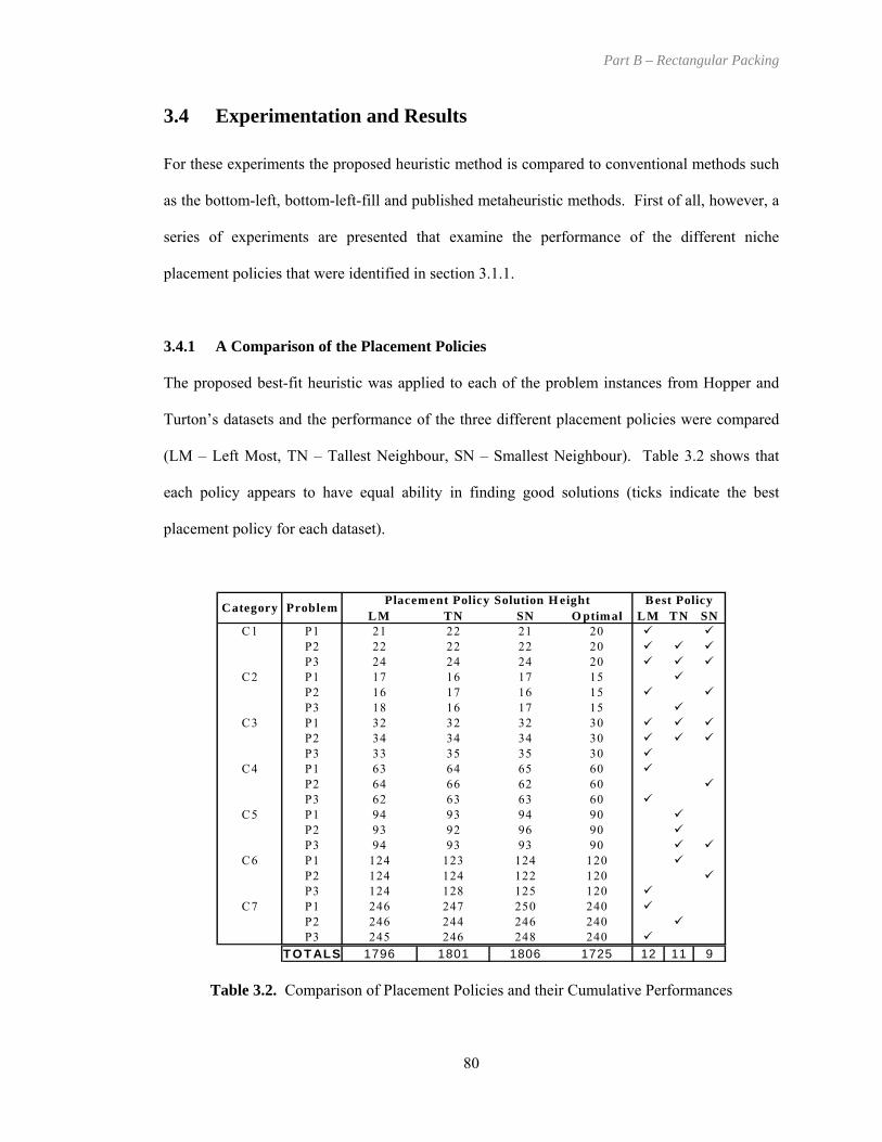
Part B – Rectangular Packing
3.4 Experimentation and Results
For these experiments the proposed heuristic method is compared to conventional methods such
as the bottom-left, bottom-left-fill and published metaheuristic methods. First of all, however, a
series of experiments are presented that examine the performance of the different niche
placement policies that were identified in section 3.1.1.
3.4.1 A Comparison of the Placement Policies
The proposed best-fit heuristic was applied to each of the problem instances from Hopper and
Turton’s datasets and the performance of the three different placement policies were compared
(LM – Left Most, TN – Tallest Neighbour, SN – Smallest Neighbour). Table 3.2 shows that
each policy appears to have equal ability in finding good solutions (ticks indicate the best
placement policy for each dataset).
LM TN SN O ptimal LM TN SNC1 P1 21 22 21 20
P2 22 22 22 20P3 24 24 24 20
C2 P1 17 16 17 15P2 16 17 16 15P3 18 16 17 15
C3 P1 32 32 32 30P2 34 34 34 30P3 33 35 35 30
C4 P1 63 64 65 60P2 64 66 62 60P3 62 63 63 60
C5 P1 94 93 94 90P2 93 92 96 90P3 94 93 93 90
C6 P1 124 123 124 120P2 124 124 122 120P3 124 128 125 120
C7 P1 246 247 250 240P2 246 244 246 240P3 245 246 248 240
T O T ALS 1796 1801 1806 1725 12 11 9
Category B est PolicyProblem Placement Policy Solution H eight
Table 3.2. Comparison of Placement Policies and their Cumulative Performances
80

Part B – Rectangular Packing
After 21 problems, all three policies perform within a cumulative height of only 10 units
difference and each policy creates an outright best solution in several of the problems. This
result validates the decision to allow all of three policies to be tried within the heuristic. As an
illustrative example, Figure 3.7 shows the solutions obtained by each placement policy with
problem C2P3 from (Hopper and Turton, 2001). The problem has 25 shapes and an optimal
solution of 15. The leftmost placement policy obtains a solution with a height of 18. The tallest
neighbour policy obtains a height of 16. The smallest neighbour policy achieves a height of 17.
a) b) c)
Figure 3.7. The solutions achieved by each of the placement policies: a) Leftmost, b) Tallest
Neighbour, and c) Smallest Neighbour on problem C2P3 from Hopper and Turton (2001) [110]
3.4.2 Comparison against Bottom-Left and Bottom-Left-Fill Algorithms
In Hopper and Turton’s comparison of bottom-left and bottom-left-fill algorithms, bottom-left-
fill produced the better packings although it took additional computation time. Also, the use of
pre-ordering shapes by decreasing width or decreasing height gave better quality solutions. As a
different quality measure is being used to that of Hopper and Turton, involving the total height
of the packing and not the density of the packing, the bottom-left and bottom-left-fill algorithms
have been implemented and tested using Hopper’s data. Table 3.3 shows that the bottom-left-
fill heuristic performs better than bottom-left and that the proposed best-fit heuristic outperforms
bottom-left-fill in all but two of the instances even when pre-ordering is allowed (DW =
decreasing width, DH = decreasing height, for unsorted random sequences are applied and the
average is taken). The best solutions are shown in bold type.
81

Part B – Rectangular Packing
Problem P1 P2 P3 P1 P2 P3 P1 P2 P3 P1 P2 P3 P1 P2 P3 P1 P2 P3 P1 P2 P3
BL 45 40 35 53 80 67 40 43 40 32 37 30 27 32 30 33 39 34 22 41 31BL-DW 30 20 20 13 27 27 10 20 17 17 22 22 16 18 13 22 25 18 16 19 17BL-DH 15 10 5 13 73 13 10 10 13 12 13 6.7 4.4 10 7.8 8.3 8.3 9.2 5 10 7.1
BLF 30 35 25 47 73 47 37 50 33 25 25 27 20 23 21 20 18 21 15 20 17BLF-DW 10 15 15 13 20 20 10 13 13 10 5 10 5.6 6.7 5.6 5 4.2 4.2 4.6 3.3 2.9BLF-DH 10 10 5 13 73 13 10 6.7 13 10 5 5 4.4 5.6 4.4 5 2.5 6.7 3.8 2.9 3.8NEW BF 5 10 20 6.7 6.7 6.7 6.7 13 10 5 3.3 3.3 3.3 2.2 3.3 2.5 1.7 3.3 2.9 1.7 2.1
C5 C6 C7C1 C2 C3 C4
No. of Rectangles
16 17 16 25 25 25 28 29 28 49 49 49 72 73 72 197 29697 97 97 196
Table 3.3. Comparison of the best-fit heuristic to bottom left and bottom-left-fill heuristics
(percentage over optimal)
3.4.3 Comparison against Metaheuristic Approaches
Hopper and Turton also show that the best packings are achieved when using the bottom-left-fill
algorithm along with a metaheuristic/evolutionary algorithm (simulated annealing or genetic
algorithm). Both of these algorithms were implemented to obtain a comparison with the new
best-fit heuristic. The metaheuristics both operate on the rectangle input sequence which is then
decoded into a layout using the bottom-left-fill placement heuristic. The fitness is based on two
distinct evaluators, a primary evaluator of the height of the layout and a secondary evaluator
based on the sheet area used. This is necessary in order to distinguish packings with identical
heights. The metaheuristics was allowed 5 runs on each problem.
Genetic Algorithm / Bottom-Left-Fill Decoder (GA+BLF)
A genetic algorithm approach was implemented with a population size of 50 and generation size
of 1000. Initially, each member of the population is a random ordering and orientation of the
input rectangles. At each generation, the sequences are decoded using bottom-left-fill to obtain
layouts. To improve the population after each generation, two parents are selected using linearly
normalised roulette wheel selection and then partially matched crossover is applied with a
probability of 60%. Two mutations are used with each occurring with a probability of 3%. The
82

Part B – Rectangular Packing
first mutation randomly swaps two rectangles within an input sequence and the second for the
flipping of a random rectangle’s orientation. Elitism is also used to preserve the best two
solutions of the population and the others are replaced by the children. The best solution seen
during the search is returned. The search parameters were set through initial experimentation.
Simulated Annealing / Bottom-Left-Fill Decoder (SA+BLF)
Simulated annealing was implemented and allowed 50000 iterations (same as the genetic
algorithm method). The initial solution is a randomly generated input sequence. To move to a
new candidate solution one of three neighbourhood operators are randomly chosen: i) swaps the
orientation of a randomly chosen rectangle, ii) moves a randomly chosen rectangle to a random
position, iii) swaps two randomly chosen rectangles. The starting temperature was calculated
based on the total area of the input rectangles for each problem. A geometric cooling schedule
of 0.9999 is applied after each iteration. If there is no improvement for 10 consecutive
iterations, the temperature is heated by applying a 1.01 times increase to the temperature. This
scheme has the effect of cooling to about a 10% acceptance rate where the search remains until
completion. After 50000 iterations, the best solution found during the process is returned. The
parameters for the simulated annealing metaheuristic were chosen through initial
experimentation.
3.4.4 Experiments on Published Data
Table 3.4 shows the resultant solutions from using the metaheuristic methods and the new best-
fit heuristic with test problems from the literature. For the metaheuristics, all times shown
indicate the time taken to achieve the solution and not the time taken to complete the run.
Therefore, the total time taken to finish the search will be of a longer duration. All experiments
were performed on a PC with an 850MHz CPU and 128MB RAM. For all instances the best
solution is shown in bold.
83

Part B – Rectangular Packing
Best Worst Time(s) Best Worst Time(s) Sol. Time(s) abs. % impv. abs. % impv.P1 16 20 20 21 3.4 20 21 1.1 21 <0.01 -1 -5.0% -1 -5.0%P2 17 20 21 21 0.5 21 21 0.8 22 <0.01 -1 -4.8% -1 -4.8%P3 16 20 20 21 7.1 20 21 0.8 24 <0.01 -4 -20.0% -4 -20.0%P1 25 15 16 16 1.3 16 16 6.5 16 <0.01 0 0% 0 0%P2 25 15 16 16 2.2 16 16 13.9 16 <0.01 0 0% 0 0%P3 25 15 16 16 1.0 16 16 13.6 16 <0.01 0 0% 0 0%P1 28 30 32 32 7.4 32 33 20.3 32 <0.01 0 0% 0 0%P2 29 30 32 32 12.4 32 32 22.5 34 <0.01 -2 -6.3% -2 -6.3%P3 28 30 32 32 11.6 32 33 18.3 33 <0.01 -1 -3.1% -1 -3.1%P1 49 60 64 64 35 64 64 65 63 <0.01 1 1.6% 1 1.6%P2 49 60 63 64 48 64 64 46 62 <0.01 1 1.6% 2 3.1%P3 49 60 62 63 61 63 64 70 62 <0.01 0 0% 1 1.6%P1 72 90 95 95 236 94 95 501 93 0.01 2 2.1% 1 1.1%P2 73 90 95 96 440 95 96 285 92 0.01 3 3.2% 3 3.2%P3 72 90 95 96 150 95 95 425 93 0.01 2 2.1% 2 2.1%P1 97 120 127 127 453 127 128 854 123 0.01 4 3.1% 4 3.1%P2 97 120 126 127 866 126 128 680 122 0.01 4 3.2% 4 3.2%P3 97 120 126 127 946 126 126 912 124 0.01 2 1.6% 2 1.6%P1 196 240 255 255 4330 255 256 4840 247 0.01 8 3.1% 8 3.1%P2 197 240 251 253 5870 253 253 5100 244 0.01 7 2.8% 9 3.6%P3 196 240 254 255 5050 255 255 6520 245 0.01 9 3.5% 10 3.9%P1 25 100 108.2 109.5 185 109.3 110.9 192 107.4 0.02 0.8 0.7% 1.9 1.7%P2 50 100 112.0 113.5 956 112.6 113.3 1358 108.5 0.01 3.5 3.1% 4.1 3.6%P3 100 100 113.0 114.0 2580 113.3 113.8 4130 107.0 0.01 6.0 5.3% 6.3 5.6%P4 200 100 113.2 114.0 1.6x10⁴ 113.4 113.8 2.3x10⁴ 105.3 0.03 7.9 7.0% 8.1 7.1%P5 500 100 111.9 112.3 5.1x10⁴ 111.9 112.2 7.3x10⁴ 103.5 0.08 8.4 7.5% 8.4 7.5%P6 1000 100 - - - - - - 103.7 0.26P1 25 100 106.7 108.4 148 109.6 110.8 122 110.1 0.04 -3.4 -3.2% -0.5 -0.5%P2 50 100 107.0 108.0 2417 108.7 109.5 1010 113.8 0.24 -6.8 -6.4% -5.1 -4.7%P3 100 100 109.0 110.1 4190 109.0 111.2 6865 107.3 0.15 1.7 1.6% 1.7 1.6%P4 200 100 108.8 109.0 1.6 x10⁴ 110.3 111.3 2.7x10⁴ 104.1 0.33 4.7 4.3% 6.2 5.6%P5 500 100 111.1 111.5 8.8x10⁴ 112.4 113.0 1.4x10⁵ 103.7 0.19 7.4 6.7% 8.7 7.7%P6 1000 100 - - - - - - 102.8 0.23
P1 50 400 400 400 5.7 400 400 6.4 400 0.01 0 0% 0 0%
No. of Shapes
Opt. Height
GAbest - BF SAbest - BFBest-Fit
Hop
per
and
Tur
ton
(200
1)
C1
C2
C3
C4
C5
C6
C7
SA+BLF
Ramesh Babu (1999)
Val
enzu
ela
and
Wan
g (2
001)
Nice
Path
GA+BLFData Set Cat. Problem
Table 3.4. Comparison of the Best-Fit heuristic against the metaheuristic methods (GA+BLF,
SA+BLF)
The final columns of table 3.4 show that the best-fit heuristic equals or outperforms both the
GA+BLF and the SA+BLF metaheuristic methods on most of the data. On closer inspection of
the cases where best-fit cannot better the metaheuristic methods, we see that this occurs on
problems involving fewer shapes. It seems that with up to around 50 shapes, which are small
problems, in general the metaheuristic methods produce the better solutions. As there are fewer
possible sequences of shapes, they are able to evaluate a larger area within the search space and,
are therefore, able to produce better solutions. On large problems, where there are more than 50
shapes to be packed, the best-fit heuristic provides the better solutions, in general. Figure 3.8
shows the best-fit solution to the problem given in (Ramesh Babu and Ramesh Babu, 1999).
84

Part B – Rectangular Packing
Figure 3.8. The resultant packing of the best-fit heuristic with Ramesh Babu’s data.
With Ramesh Babu’s data, the Best-Fit heuristic obtains a solution of 40mm which equals the
height returned from the implemented metaheuristic methods and Ramesh Babu’s genetic
method. It gives a better result than the solution of Jakobs’ genetic method, which only
achieved a solution of height of 45mm (Ramesh Babu and Ramesh Babu, 1999). The execution
time of Ramesh Babu’s genetic algorithm is given as 521s on a 100MHz processor. However,
the solution obtained using best-fit was achieved in 0.01 seconds. Although the best-fit solution
was achieved on a significantly faster processor, the reduction in the time required is significant.
a) b) c)
Figure 3.9. A comparison of the a) best-fit heuristic, b) bottom-left-fill + GA and c) bottom-
left-fill + SA using problem C7P2 from Hopper and Turton (2001) [110]
85

Part B – Rectangular Packing
As an illustrative example a comparison of the solutions obtained by each of the examined
methods is given in figure 3.9 using problem C7P2 of 197 shapes and where the optimal
solution is known to be 240 from (Hopper and Turton, 2001). Best-fit achieves a solution with
height of 244, GA+BLF finds a solution with height 251 using a population of 50 and several
runs of 1000 generation each, SA+BLF finds a solution with height 253 after several 50000
eration runs.
old.
The execution times from tables 3.4 and 3.5 indicate that the best-fit heuristic can reach good
solutions in significantly quicker time than the other methods. In fact, on the newly generated
problems in table 3.5, best-fit completes all solutions in a combined time of less than 2 seconds.
Due to the use of populations with the genetic algorithm and neighbourhood functions with
simulated annealing, there is an increase in execution time (because of their associated
operations).
it
With Valenzuala’s floating point based data, the best-fit heuristic performed consistently better
than the other methods. Due to the floating point nature of the data and the integer based
implementations, all methods took longer to execute than similarly sized integer problems due to
scaling. However, because the best-fit heuristic is a one-pass method, the overhead is not
exceptional.
3.4.5 Experiments on Randomly Generated Data
In many real world industrial applications there are time constraints and economic reasons for
reaching good solutions quickly, so to compare the various methods we should consider the time
used in finding the solution. Table 3.5 uses the newly presented data sets to show both solution
quality and difference in time taken to find the solution. Once again the best solutions are
presented in b
86

Part B – Rectangular Packing
Result Time(s) Result Time(s) Result Time(s) Abs. % imp. Abs. % imp.N1 10 40 40 1.02 40 0.24 45 <0.01 -5 -12.5% -5 -12.5%N2 20 50 51 9.2 52 8.14 53 <0.01 -2 -3.9% -1 -1.9%N3 30 50 52 2.6 52 39.5 52 <0.01 0 0% 0 0%N4 40 80 83 12.6 83 84 83 <0.01 0 0% 0 0%N5 50 100 106 52.3 106 228 105 0.01 1 0.9% 1 0.9%N6 60 100 103 261 103 310 103 0.01 0 0% 0 0%N7 70 100 106 671 106 554 107 0.01 -1 -0.9% -1 -0.9%N8 80 80 85 1142 85 810 84 0.01 1 1.2% 1 1.2%N9 100 150 155 4431 155 1715 152 0.01 3 1.9% 3 1.9%N10 200 150 154 2 x 10⁴ 154 6066 152 0.02 2 1.3% 2 1.3%N11 300 150 155 8 x 10⁴ 155 3 x 10⁴ 152 0.03 3 1.9% 3 1.9%N12 500 300 313 4 x 10⁵ 312 6 x 10⁴ 306 0.06 7 2.2% 6 1.9%N13 3152 960 - - - - 964 1.37
SAbest - BFGAbest - BFProblem
GA+BLF BF HeuristicSA+BLFNo. of Shapes
Optimal Height
Table 3.5. A comparison of execution time
Figure 3.10. The resultant packing from data N13 involving 3152 rectangles. A packing of
height 964 is achieved using best-fit, which is only 4 over optimum
87

Part B – Rectangular Packing
The power of the approach that has been presented is particularly illustrated by considering the
largest of the new problems N13. Note that the GA+BLF and SA+BLF methods were unable to
complete N13, due to its excessive time requirements (extrapolated to approximately 26-40
weeks of execution time). However, the best-fit heuristic was able to pack the 3152 shapes in
less than two seconds and gave a solution of 964, which is only 4 units above optimal. The
solution is presented in figure 3.10.
3.5 Summary
this chapter, a new heuristic based on a best fit methodology has been described and an
most of the problems. The new
heuristic has also produced better quality packings than the metaheuristic hybrids when given
problems of 50 shapes or more. Also, solutions were obtained in a significantly shorter period
of time by several orders of magnitude. The method also performs very well with datasets
containing similar sized rectangles and ones containing differing sized rectangles (such as the
problems represented by Valenzuela’s data). In Hopper and Turton (2001) [110], the authors
concluded that the methods that yielded the best results were GA+BLF and SA+BLF. It has
been demonstrated that, even with extremely large problems, the proposed best-fit heuristic is
able to outperform currently published and established heuristic and metaheuristic methods to
produce solutions that are very close to optimal using very small execution times.
In the next chapter, the best-fit placement heuristic is modified to perform accurately with
floating point data and the heuristic is hybridised with bottom-left-fill metaheuristic methods to
enable the automatic generation of even better quality layouts.
In
efficient implementation of the heuristic has been produced. Using data provided by other
researchers in the field of cutting and packing, the new best-fit heuristic has produced better
results than the bottom-left and bottom-left-fill heuristics for
88
Part B – Rectangular Packing
CHAPTER FOUR
A Metaheuristic Hybrid Approach
In this chapter, a hybridised best-fit / bottom-left-fill strategy is proposed. The chapter begins
with a broad overview of the approach and then a description of the modifications that are made
to the representation of the skyline from the previous chapter. It then describes how the best-fit
and bottom-left-fill elements can be combined to produce a strategy that outperforms other
approaches from the literature. Finally, comparisons are drawn to the previous literature and the
best-fit heuristic presented in chapter three on the set of literature benchmark problems as
detailed in table 2.2, the new data from the previous chapter (N1 – N13) and ten more randomly
generated benchmark datasets (MT1 – MT10).
4.1 Overview of the Hybrid Metaheuristic Approach
The method that is described in this section utilises two different packing algorithms to produce
a solution for a given orthogonal packing problem. These algorithms are: the best-fit heuristic
as presented in chapter three (modified to operate on floating point data without discretisation)
and the bottom-left-fill heuristic as developed by Hopper and Turton (2001) [110]. A solution is
generated by a two-step process firstly involving the application of the best-fit heuristic to place
an initial number of rectangles onto the stock sheet. The remaining unassigned rectangles are
placed using the bottom-left-fill heuristic with different input orderings as guided by tabu,
simulated annealing and genetic algorithm based metaheuristic search procedures. The positions
of the rectangles that are assigned to the sheet in the initial best-fit stage of the process remain
fixed throughout and form the first part of the solution whereas the rectangles placed during the
89
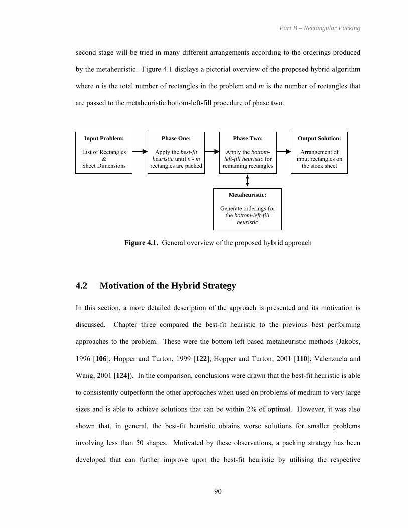
Part B – Rectangular Packing
second stage will be tried in many different arrangements according to the orderings produced
by the metaheuristic. Figure 4.1 displays a pictorial overview of the proposed hybrid algorithm
where n is the total number of rectangles in the problem and m is the number of rectangles that
are passed to the metaheuristic bottom-left-fill procedure of phase two.
Phase Two:
Apply the bottom-left-fill heuristic for remaining rectangles
Metaheuristic: Generate orderings for
the bottom-left-fill heuristic
Output Solution:
Arrangement of input rectangles on
the stock sheet
Phase One:
Apply the best-fit heuristic until n - m
rectangles are packed
Input Problem:
List of Rectangles &
Sheet Dimensions
Figure 4.1. General overview of the proposed hybrid approach
4.2 Motivation of the Hybrid Strategy
In this section, a more detailed description of the approach is presented and its motivation is
discussed. Chapter three compared the best-fit heuristic to the previous best performing
approaches to the problem. These were the bottom-left based metaheuristic methods (Jakobs,
1996 [106]; Hopper and Turton, 1999 [122]; Hopper and Turton, 2001 [110]; Valenzuela and
Wang, 2001 [124]). In the comparison, conclusions were drawn that the best-fit heuristic is able
to consistently outperform the other approaches when used on problems of medium to very large
sizes and is able to achieve solutions that can be within 2% of optimal. However, it was also
shown that, in general, the best-fit heuristic obtains worse solutions for smaller problems
involving less than 50 shapes. Motivated by these observations, a packing strategy has been
developed that can further improve upon the best-fit heuristic by utilising the respective
90

Part B – Rectangular Packing
strengths of both the best-fit heuristic and the metaheuristic bottom-left methods. The
advantages and disadvantages of the two strategies are summarised in table 4.1.
Best-Fit Heuristic
(Phase 1)
Metaheuristic Bottom-Left Methods
(Phase 2)
Advantages Disadvantages Advantages Disadvantages
Produces best published
results on a range of
medium/large standard
benchmark problems
Worse solutions
found when
problem size < 50
Optimal solutions
found on small
problems
Does not represent the
best approaches on
medium/large
problems
Fast solutions obtained
≈ 1000
rectangles/second
Arrangements at
the end of the
packing often
create holes/waste
Can execute for as
long as user allows
Similar input
sequences may
produce vastly
differing solutions
No parameters Definition of search
parameters is required
Table 4.1. Advantages and disadvantages of the best-fit heuristic and metaheuristic bottom-left
methods
Given an orthogonal stock cutting problem involving n rectangles, the best-fit heuristic is
invoked to pack the first n – m rectangles where m is the number of rectangles that are to be
carried over to phase 2. Phase 2 involves the packing of the remaining rectangles using the
metaheuristic bottom-left-fill combinatorial method for a suitable duration of time. At the
commencement of phase 2 it should be noted that we already have the foundations of a solution
because the best-fit heuristic (phase 1) has already placed a number of the rectangles on the
sheet. These rectangles will remain unchanged during the guided search procedure of phase 2.
91
Part B – Rectangular Packing
The reasoning for this approach can be seen by further examination of table 4.1. Phase 1 aims to
utilise the best-fit heuristic’s ability to produce high quality solutions in quick time. The earlier
termination of the best-fit process, before the entirety of the rectangles are packed, aims to
reduce the untidy arrangements that usually occur during the latter stages of best-fit solutions
due to the smaller number of rectangles that are available for selection. If a relatively small sub-
problem is passed to the metaheuristic method of phase 2, we can limit the problem of
excessively large search spaces therefore allowing good phase 2 partial solutions to be found
relatively quickly which can be concatenated to the partial solution of phase 1 in order to create
the overall layout. Although other factors may also be important such as sheet width or relative
size of the problem shapes, it can be seen how the proposed model aims to promote the
advantages of both methods whilst inhibiting their disadvantages.
The transition from one phase to the other is guided by the m variable. If m = 0 then all
rectangles are packed using the best-fit heuristic. However, if m >= n then only phase 2 is used
and the approach only uses the metaheuristic bottom-left-fill strategy. From the observations of
the previous chapter, the following prediction can be made: if m > 50 then the metaheuristic of
phase two will probably obtain a worse solution than if we used the standalone best-fit heuristic;
therefore an effective value for m may be somewhere in the range 0 < m < 50. In section 4.5.1
experiments are conducted to evaluate the given strategy and to examine the prediction for the
most productive value for m.
In the next two sections, 4.3 and 4.4, a new floating point representation for the best-fit skyline
is described and, because the bottom-left-fill placement heuristic uses a representation utilising
placement positions rather than the skyline, a method to convert the skyline to location points is
described. Only this representation conversion is needed to enable the new hybrid approach to
function properly. All other parameter settings remain the same as in chapter three.
92

Part B – Rectangular Packing
93
0
1
2
3
4
5
0 1 2 3 4 5 6 7
4.3 Development of a Floating Point Skyline Representation
In order to achieve full accuracy within the best-fit heuristic, this chapter uses a new floating
point capable representation. This is achieved through the use of a data structure that involves a
linked list containing the location and length of skyline sub-elements. Figure 4.2 displays the
new linked list representation of the skyline constructed from four skyline elements after
packing five rectangles and raising the gap once (due to no rectangle fitting the lowest space).
8
y
x
i = 1
i = 0i = 3
i = 2
i = 0 i = 1 i = 2 i = 3 (x = 0, y = 3.763) (x = 3.224, y = 4.377) (x = 4.263, y = 2.012) (x = 5.37, y = 3.399)
length = 3.224 length = 2.783 length = 1.039 length = 1.107
Figure 4.2. Floating-point representation of the skyline
Using this new floating-point data structure the lowest location and the size of this location on
the stock sheet can be found by traversing the linked-list for the skyline element with the
smallest y component. Due to the floating-point operations and the importance of handling
mathematical processor rounding errors, this method can take up to 5 times longer than the array
based method. However, this enhancement can be justified because of the extra accuracy on
floating-point datasets (as given in Valenzuela and Wang (2001) [124]) and also because the
execution times are still less than 1 second for all but the largest of the benchmark problems.

Part B – Rectangular Packing
4.4 Best-Fit Conversion to Bottom-Left-Fill Representation
One important consideration is how the solution of the best-fit heuristic can be converted into
the considerably different representation that is used by the bottom-left-fill approach. The best-
fit heuristic produces solutions by using a data structure to maintain the ‘skyline’ or the height
profile of a layout whereas the bottom-left-fill approach requires the maintenance of height
sorted (and left to right sorted) potential location points (see figure 2.3). After phase one of this
approach, the skyline data structure can be converted to a set of potential rectangle locations for
use with bottom-left-fill by extending each subelement of the skyline leftwards until it intersects
another part of the skyline or the sheet side (see figure 4.3). The placement locations must then
be sorted in increasing y coordinate order (and sorted by left to right where y coordinates are
equal). This overall state is stored so that it can be easily revisited because it is always the
starting point for the bottom-left-fill heuristic to evaluate the rectangle sequences that are
generated by the metaheuristic search techniques.
Figure 4.3. Conversion of best-fit’s skyline into bottom-left-fill’s placement positions
Given a specific ordering of the selected rectangles, the bottom-left-fill heuristic can now
produce a layout by taking the first rectangle
of the sequence and placing it at each location
point in turn until it does not intersect with an already placed rectangle. Once a valid position is
right corners of the placed
c can place the second rectangle and
so forth until all rectangles have been placed.
found, new potential location points, given by the top left and bottom
rectangle, are added to the list of locations and the heuristi
94

Part B – Rectangular Packing
4.5 Hybrid Approach Summary
The whole process is su
Figure 4.4. A summary of the proposed strategy
mmarised pictorially in figure 4.4.
Phase 1 (until n - m rectangles have been packed)
Phase 2 (for s seconds)
Best-Fit
Heuristic
Metaheuristic Simulated Annealing
01
Initial Temperature = 3Cooling = 0.999 Reheat = 1.00
Genetic Algorithms
Module (initially seeded by
height-decreasing order)
Pop Size = 30, Elite = 5
Mutation Rates: “Swap” = 0.03 “Orientation Fli
Tabu Search
Neighbourhood SizeTabu List Size = 1000
Crossover = PMX/Order-BasedCrossover Rate = 0.6 = 5
p” = 0.03
Inputs: x, y : sheet dimensions
s : phase 2 duration
-Left-Fill
Heuristic
Phase 1 solution skyline
m rectangles
Bottom
input se
solution
quence
n : number of rectanglesm: phase switch
95

Part B – Rectangular Packing
4.6 Benchmark Test Data
In order to rigorously evaluate the proposed approach, the entire set of literature benchmark
problems (see table 2.2) and the problems introduced in the last chapter, N1-13 (see table 3.1),
are used once more. Further to these, ten new problem instances have been introduced for this
chapter which are used to examine how solution quality is affected by different phase switch
values for m and longer search durations in section 4.5.4.
The first five of these problems, MT1-MT5, offer more realistic industrial problems because the
optimal solutions are not known (lower bounds of feasibility are calculated by dividing the total
area of the rectangles by the sheet width). The last five problems, MT5-MT10, have been
created through the dissection of a larger rectangular object and so for these problems the
optimal height is known. Table 4.2 summarises the first five datasets, MT1-MT5, for which the
optimal packing is unknown. The new datasets, for which optimal solutions are known, MT6-
MT10, are given in table 4.3. The data for all of these problems can be found in appendix C.
New Test
Problem
Number of
Rectangles
Lower Bound
Height
Object
Dimensions
MT1
MT2
MT3
MT4
MT5
100
150
200
300
500
492.63
760.90
767.31
1174.94
1264.86
400 x 600
300 x 900
400 x 900
600 x 1300
800 x 1400
Table 4.2. New test data with unknown optimal heights
New Test
Problem
Number of
Rectangles
Optimal
Height
Object
Dimensions
MT6
MT7
MT8
MT9
MT10
100
150
200
300
500
500
500
800
800
800
400 x 500
400 x 500
500 x 800
600 x 800
700 x 800
Table 4.3. New test data with known optimal heights
96

Part B – Rectangular Packing
4.7 Experimentation and Results
In this section, the results of the proposed method are compared with the results from the
approach of the previous chapter. Previously, a singular evaluation method of the total layout
height was used to compare the approaches. In order to make comparisons in this chapter, a
dual evaluation approach is introduced. This involves the height of the solution obtained (as
before) but a secondary measure of the total area underneath the skyline. The main objective is
to minimise the height of the packing but, as several different arrangements may have identical
heights, the area under the skyline can also be important because it quantifies the amount of
wasted space. If a smaller area is required, it means that the rectangles have been packed more
densely and therefore the solution has less wasted material and, hence, more of the sheet may be
reused in future cutting operations.
As an example, two arrangements that produce solutions of identical height but differing skyline
areas are shown in figure 4.5. The solution on the right in figure 4.5 is intuitively (and visually)
more desirable as it requires less sheet area so there is less trim-loss and more of the sheet could
normally be reused in future cutting processes.
H
Figure 4.5. Two possible solutions of identical total he
evaluations
97
= 36, Area = 1800
H = 36, Area = 2156ight but vastly different skyline area
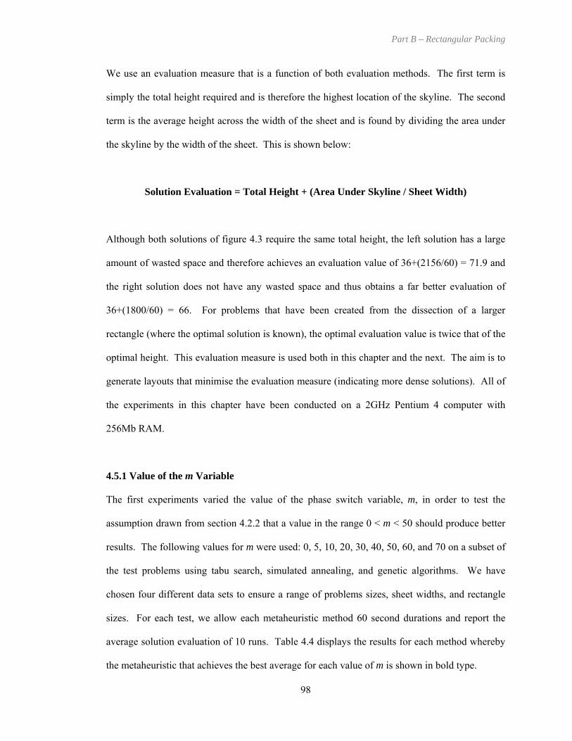
Part B – Rectangular Packing
We use an evaluation measure that is a function of both evaluation methods. The first term is
simply the total height required and is therefore the highest location of the skyline. The second
term is the average height across the width of the sheet and is found by dividing the area under
the skyline by the width of the sheet. This is shown below:
Solution Evaluation = Total Height + (Area Under Skyline / Sheet Width)
Although both solutions of figure 4.3 require the same total height, the left solution has a large
amount of wasted space and therefore achieves an evaluation value of 36+(2156/60) = 71.9 and
the right solution does not have any wasted space and thus obtains a far better evaluation of
36+(1800/60) = 66. For problems that have been created from the dissection of a larger
rectangle (where the optimal solution is known), the optimal evaluation value is twice that of the
optimal height. This evaluation measure is used both in this chapter and the next. The aim is to
generate layouts that minimise the evaluation measure (indicating more dense solutions). All of
the experiments in this chapter have been conducted on a 2GHz Pentium 4 computer with
256Mb RAM.
4.5.1 Value of the m Variable
The first experiments varied the value of the phase switch variable, m, in order to test the
assumption drawn from section 4.2.2 that a value in the range 0 < m < 50 should produce better
results. The following values for m were used: 0, 5, 10, 20, 30, 40, 50, 60, and 70 on a subset of
the test problems using tabu search, simulated annealing, and genetic algorithms. We have
chosen four different data sets to ensure a range of problems sizes, sheet widths, and rectangle
sizes. For each test, we allow each metaheuristic method 60 second durations and report the
average solution evaluation of 10 runs. Table 4.4 displays the results for each method whereby
the metaheuristic that achieves the best average for each value of m is shown in bold type.
98

Part B – Rectangular Packing
Eval % Over Opt Eval % Over Opt Eval % Over Opt0 244.01 1.67 244.01 1.67 244.01 1.675 243.98 1.66 243.98 1.66 243.98 1.66
10 243.88 1.62 243.88 1.62 243.88 1.6220 242.70 1.13 242.69 1.12 242.73 1.1430 242.66 1.11 242.71 1.13 243.15 1.3140 243.03 1.26 243.47 1.45 244.08 1.7050 243.57 1.49 244.05 1.69 244.95 2.0660 243.25 1.35 244.54 1.89 245.95 2.4870 243.64 1.52 245.10 2.13 246.91 2.880 489.12 1.90 489.12 1.90 489.12 1.905 489.12 1.90 489.12 1.90 489.12 1.90
10 489.71 2.02 489.71 2.02 489.71 2.0220 487.72 1.61 487.65 1.59 487.71 1.6130 487.70 1.60 487.74 1.61 488.11 1.6940 487.59 1.58 487.69 1.60 488.50 1.7750 488.10 1.69 488.58 1.79 488.26 1.7260 487.63 1.59 488.89 1.85 489.29 1.9370 488.08 1.68 490.10 2.10 491.30 2.350 209.63 4.82 209.63 4.82 209.63 4.825 209.54 4.77 209.54 4.77 209.54 4.77
10 209.11 4.55 209.11 4.55 209.11 4.5520 207.50 3.75 207.14 3.57 207.64 3.8230 207.48 3.74 207.38 3.69 208.07 4.0340 207.81 3.91 208.21 4.10 208.39 4.1950 208.01 4.00 208.51 4.26 208.94 4.4760 208.52 4.26 209.80 4.90 209.41 4.7170 208.79 4.39 209.78 4.89 210.19 5.100 1557.27 2.33 1557.27 2.33 1557.27 2.335 1552.70 2.03 1552.70 2.03 1552.70 2.03
10 1552.77 2.03 1552.77 2.03 1552.77 2.0320 1553.47 2.08 1549.90 1.85 1553.30 2.0730 1544.01 1.46 1544.06 1.46 1545.14 1.5340 1546.37 1.61 1544.71 1.51 1548.27 1.7450 1548.63 1.76 1547.78 1.71 1556.38 2.2760 1548.67 1.77 1549.93 1.85 1557.56 2.3570 1549.80 1.84 1552.92 2.04 1561.85 2.63
SAAverage Evaluation (10 runs)
GAProblemm
ValueOptim al
Evaluation
Hopper C7P1
(196 shapes)
Valenzuela Nice P4
(200 shapes)
New Data MT2
(150 shapes)
Tabu
Hopper C6P1
(97 shapes)240
480
200
Optimal Not Know n
(Low er Bound Eval =1521.8)
Table 4.4. Varying the phase switch parameter, m
From these results, the best setting for m is consistently between 20 and 40 for these sets of data
and a 60 second run. The average result returned over the range of m values is shown in the
graphs of figure 4.6. At lower values, the metaheuristics are not given enough shapes to be able
to make significant improvements on the best-fit result. Larger values of m seem to impair the
metaheuristics because of the larger search spaces but may produce better solutions if a greater
execution time were allowed (see sections 4.5.3 and 4.5.4). Other problem specific factors may
also be important such as the sheet width, rectangle sizes, and more importantly the quantity of
wasted space that is inherited from the result given by the best-fit heuristic. Due to these results,
the value of m is fixed at 30 for the experiments on the literature benchmark problems in section
4.5.2.
99

Part B – Rectangular Packing
1
1.5
2
2.5
3
0 5 10 20 30 40 50 60 70m
%overopt TABU
SAGA
Hopper - C6P1
1.5
1.7
1.9
2.1
2.3
2.5
0 5 10 20 30 40 50 60 70m
%overopt
TABUSAGA
Hopper - C7P1
1.3
1.7
2.1
2.5
2.9
0 5 10 20 30 40 50 60 70m
%overopt TABU
SAGA
New Data - MT2
3.5
4
4.5
5
5.5
0 5 10 20 30 40 50 60 70m
%overopt
TABUSAGA
Valenzuela - Nice P4
Figure 4.6. Comparison graphs of the percentage above optimal when varying phase switch
parameter, m
4.5.2 Evaluation of the Hybrid Metaheuristic Approach with the Benchmark Problems of
the Literature
The second set of experiments aimed to compare the proposed hybrid metaheuristic method to
other approaches from the literature including the standalone best-fit heuristic as proposed in
chapter three and Burke, Kendall, and Whitwell (2004) [1] and the metaheuristic bottom-left-fill
methods proposed in Hopper and Turton (2001) [110]. For all the experiments in this section m
remains fixed at 30 rectangles (given the results of section 4.5.1) and 60 seconds are allowed for
the metaheuristic search of phase 2. The best and average solution of ten runs is given for all the
problems from the literature in table 4.6. The best solution for each method is given in the final
columns as a percentage over optimal and the best method is highlighted in bold type.
100

Height Area Eval. Height Area Eval. Height Area Eval. Height Area Eval.P1 16 20 40 21 410 41.50 20 400 40.00 40.71 20 400 40.00 40.00 20 400 40.00 40.60 3.75 0.00 0.00 0.00P2 17 20 40 22 400 42.00 21 400 41.00 41.02 20 400 40.00 40.50 21 400 41.00 41.00 5.00 2.50 0.00 2.50P3 16 20 40 24 400 44.00 20 400 40.00 40.61 20 400 40.00 40.00 20 400 40.00 40.70 10.00 0.00 0.00 0.00P1 25 15 30 16 609 31.23 16 600 31.00 31.02 16 600 31.00 31.00 16 600 31.00 31.02 4.08 3.33 3.33 3.33P2 25 15 30 16 600 31.00 16 600 31.00 31.01 16 600 31.00 31.00 16 600 31.00 31.00 3.33 3.33 3.33 3.33P3 25 15 30 16 604 31.10 16 600 31.00 31.00 16 600 31.00 31.00 16 600 31.00 31.01 3.67 3.33 3.33 3.33P1 28 30 60 32 1814 62.23 31 1810 61.17 61.95 31 1818 61.30 61.59 31 1823 61.38 61.98 3.72 1.94 2.17 2.31P2 29 30 60 34 1801 64.02 32 1800 62.00 62.06 31 1814 61.23 61.72 32 1809 62.15 62.49 6.69 3.33 2.06 3.58P3 28 30 60 33 1806 63.10 31 1826 61.43 61.98 31 1808 61.13 61.46 31 1826 61.43 62.15 5.17 2.39 1.89 2.39P1 49 60 120 63 3623 123.38 62 3622 122.37 122.51 61 3621 121.35 122.08 62 3623 122.38 122.75 2.82 1.97 1.13 1.99P2 49 60 120 62 3621 122.35 62 3617 122.28 122.46 61 3618 121.30 122.20 62 3624 122.40 122.90 1.96 1.90 1.08 2.00P3 49 60 120 62 3621 122.35 61 3616 121.27 122.01 61 3608 121.13 121.53 62 3610 122.17 122.34 1.96 1.06 0.94 1.81P1 72 90 180 93 5444 183.73 92 5415 182.25 182.40 91 5419 181.32 182.33 92 5432 182.53 182.74 2.07 1.25 0.73 1.41P2 73 90 180 92 5413 182.22 92 5414 182.23 182.52 91 5410 181.17 182.18 92 5422 182.37 182.94 1.23 1.24 0.65 1.31P3 72 90 180 93 5469 184.15 92 5437 182.62 182.72 92 5438 182.63 182.79 92 5446 182.77 182.91 2.31 1.45 1.46 1.54P1 97 120 240 123 9681 244.01 122 9648 242.60 242.75 122 9652 242.65 242.80 122 9678 242.98 243.33 1.67 1.08 1.10 1.24P2 97 120 240 122 9632 242.40 121 9632 241.40 241.93 121 9632 241.40 241.42 121 9634 241.43 241.84 1.00 0.58 0.58 0.59P3 97 120 240 124 9664 244.80 122 9645 242.56 242.60 122 9647 242.59 242.63 122 9649 242.61 242.68 2.00 1.07 1.08 1.09P1 196 240 480 246 38899 489.12 245 38818 487.61 487.70 244 38839 486.74 487.75 245 38855 487.84 488.47 1.90 1.59 1.40 1.63P2 197 240 480 244 38715 485.97 244 38663 485.64 485.73 244 38667 485.67 487.02 244 38699 485.87 486.70 1.24 1.18 1.18 1.22P3 196 240 480 245 38864 487.90 245 38853 487.83 488.74 245 38850 487.81 488.17 245 38858 487.86 488.75 1.65 1.63 1.63 1.64P1 25 100 200 107.99 10267.7 210.67 106.93 10242.0 209.35 210.70 104.024 10049.5 204.52 207.25 108.42 10190.1 210.33 211.30 5.33 4.67 2.26 5.16P2 50 100 200 109.69 10423.8 213.93 106.64 10388.5 210.53 211.10 104.413 10221.0 206.62 208.24 106.87 10409.4 210.97 212.59 6.97 5.26 3.31 5.48P3 100 100 200 107.92 10273.2 210.65 105.23 10276.1 207.99 208.45 105.04 10335.0 208.39 208.69 105.94 10336.3 209.31 211.11 5.33 4.00 4.19 4.65P4 200 100 200 106.89 10274.1 209.63 104.21 10288.1 207.09 207.39 104.743 10266.7 207.41 207.59 104.89 10307.8 207.97 208.90 4.82 3.55 3.71 3.98P5 500 100 200 103.39 10195.4 205.35 103.18 10193.4 205.11 205.89 103.507 10199.3 205.50 206.01 103.48 10197.7 205.46 206.25 2.67 2.56 2.75 2.73P6 1000 100 200 103.84 10267.6 206.52 103.80 10268.2 206.48 206.73 103.756 10269.8 206.45 206.72 103.80 10271.7 206.52 207.02 3.26 3.24 3.23 3.26P1 25 100 200 110.19 10253.7 212.73 105.82 10345.9 209.28 209.87 103.09 10038.3 203.47 207.21 108.17 10250.6 210.68 212.88 6.36 4.64 1.74 5.34P2 50 100 200 113.65 10285.1 216.50 103.66 10080.2 204.46 204.79 103.4 10060.9 204.01 204.59 103.66 10085.0 204.51 204.92 8.25 2.23 2.00 2.26P3 100 100 200 106.75 10180.6 208.56 104.73 10084.9 205.58 206.47 103.037 10125.7 204.29 205.92 104.37 10217.6 206.55 207.52 4.28 2.79 2.15 3.27P4 200 100 200 104.12 10157.4 205.70 103.53 10058.3 204.11 204.51 103.419 10116.1 204.58 204.63 103.85 10068.3 204.53 204.73 2.85 2.06 2.29 2.26P5 500 100 200 103.81 10189.0 205.70 103.15 10210.4 205.25 205.38 103.479 10200.1 205.48 205.60 103.41 10209.0 205.50 206.22 2.85 2.63 2.74 2.75P6 1000 100 200 103.09 10173.0 204.82 102.80 10162.1 204.42 204.69 102.867 10165.0 204.52 204.68 102.90 10169.1 204.59 205.11 2.41 2.21 2.26 2.30P1 50 375 750 400 378125 778.13 400 367875 767.88 767.88 400 367875 767.88 767.88 400 367875 767.88 767.96 3.75 2.38 2.38 2.38N1 10 40 80 45 1800 90.00 40 1600 80.00 80.00 40 1600 80.00 80.00 40 1600 80.00 80.00 12.50 0.00 0.00 0.00N2 20 50 100 53 1542 104.40 50 1500 100.00 101.68 50 1500 100.00 101.68 50 1500 100.00 102.01 4.40 0.00 0.00 0.00N3 30 50 100 52 1525 102.83 51 1503 101.10 101.51 51 1500 101.00 101.32 52 1508 102.27 102.13 2.83 1.10 1.00 2.27N4 40 80 160 86 6547 167.84 83 6437 163.46 163.70 82 6455 162.69 163.50 83 6443 163.54 163.82 4.90 2.16 1.68 2.21N5 50 100 200 105 10154 206.54 103 10124 204.24 204.34 103 10122 204.22 204.29 104 10112 205.12 205.48 3.27 2.12 2.11 2.56N6 60 100 200 102 5061 203.22 102 5047 202.94 202.95 102 5047 202.94 202.94 102 5047 202.94 202.97 1.61 1.47 1.47 1.47N7 70 100 200 108 8230 210.88 105 8094 206.18 206.26 104 8117 205.46 205.97 104 8113 205.41 206.30 5.44 3.09 2.73 2.71N8 80 80 160 83 8116 164.16 82 8097 162.97 162.97 82 8097 162.97 162.97 82 8097 162.97 162.97 2.60 1.86 1.86 1.86N9 100 150 300 152 7556 303.12 152 7544 302.88 317.88 152 7544 302.88 317.88 152 7544 302.88 317.92 1.04 0.96 0.96 0.96
N10 200 150 300 152 10567 302.96 152 10570 303.00 303.00 152 10570 303.00 303.00 152 10570 303.00 303.00 0.99 1.00 1.00 1.00N11 300 150 300 153 10586 304.23 153 10586 304.23 304.23 153 10586 304.23 304.23 153 10586 304.23 304.23 1.41 1.41 1.41 1.41N12 500 300 600 306 30431 610.31 306 30431 610.31 610.31 306 30431 610.31 610.31 306 30431 610.31 610.31 1.72 1.72 1.72 1.72N13 3152 960 1920 964 615637 1925.9 964 615637 1925.9 1925.9 964 615629 1925.9 1925.9 964 615629 1925.9 1925.9 0.31 0.31 0.31 0.31
Cat.
C7
C5
C2
C3
C4
Avr. Eval
Bur
ke, K
enda
ll, W
hitw
ell
(2
004)
Ramesh Babu
Val
enzu
ela
and
Wan
g (2
001)
Nic
ePa
th
C1
Hop
per
and
Tur
ton
(200
1)
Data Set
C6
Prob No. Shapes
Opt Height
Best-FitOpt Eval
Best-Fit + Metaheuristic Bottom-Left-Fill
Solution ObtainedGenetic Algorithms
Best Solution Avr. EvalBest SolutionTabu Search
Avr. Eval
Simulated AnnealingBest Solution
Best Sol. % Over Optimal
BF BF + Tabu
BF + SA BF + GA
Table 4.5. Comparison of new hybrid approach to the best-fit heuristic using test problems from the literature

Height Area Eval. Height Area Eval. Height Area Eval. Height Area Eval.P1 16 20 40 20 400 40.00 40.82 20 400 40.00 40.00 20 400 40.00 40.71 20 400 40.00 40.00P2 17 20 40 21 400 41.00 41.00 20 400 40.00 40.73 21 400 41.00 41.02 20 400 40.00 40.50P3 16 20 40 20 400 40.00 40.50 20 400 40.00 40.10 20 400 40.00 40.61 20 400 40.00 40.00P1 25 15 30 16 600 31.00 31.00 15 600 30.00 30.90 16 600 31.00 31.02 16 600 31.00 31.00P2 25 15 30 16 600 31.00 31.00 16 600 30.00 31.00 16 600 31.00 31.01 16 600 31.00 31.00P3 25 15 30 16 600 31.00 31.00 16 600 30.00 31.00 16 600 31.00 31.00 16 600 31.00 31.00P1 28 30 60 31 1810 61.17 61.85 31 1800 61.00 61.36 31 1810 61.17 61.95 31 1818 61.30 61.59P2 29 30 60 32 1800 62.00 62.20 31 1801 61.02 61.63 32 1800 62.00 62.06 31 1801 61.02 61.59P3 28 30 60 31 1822 61.37 61.96 31 1810 61.17 61.52 31 1826 61.43 61.98 31 1808 61.13 61.46P1 49 60 120 62 3617 122.28 122.91 62 3643 122.72 123.92 62 3622 122.37 122.51 61 3621 121.35 122.08P2 49 60 120 62 3617 122.28 122.33 61 3620 121.33 122.66 62 3617 122.28 122.46 61 3618 121.30 122.20P3 49 60 120 62 3612 122.20 122.32 62 3619 122.32 122.43 61 3616 121.27 122.01 61 3608 121.13 121.53P1 72 90 180 92 5415 182.25 183.13 92 5462 183.03 183.84 92 5415 182.25 182.40 91 5419 181.32 182.33P2 73 90 180 92 5407 182.12 182.48 91 5422 181.37 183.24 92 5414 182.23 182.52 91 5410 181.17 182.18P3 72 90 180 92 5431 182.52 183.02 93 5460 184.00 184.12 92 5437 182.62 182.72 92 5438 182.63 182.79P1 97 120 240 122 9695 243.19 243.75 122 9694 243.18 244.32 122 9648 242.60 242.75 122 9652 242.65 242.80P2 97 120 240 122 9635 242.44 242.99 122 9668 242.85 244.20 121 9632 241.40 241.93 121 9632 241.40 241.42P3 97 120 240 122 9726 243.58 244.14 123 9703 244.30 244.52 122 9645 242.56 242.60 122 9647 242.59 242.63P1 196 240 480 246 38741 488.13 488.47 245 38915 488.22 489.39 245 38818 487.61 487.70 244 38839 486.74 487.75P2 197 240 480 244 38767 486.29 487.12 246 38873 487.72 488.13 244 38663 485.64 485.73 244 38667 485.67 487.02P3 196 240 480 245 38864 487.90 488.40 245 38899 488.12 488.52 245 38853 487.83 488.74 245 38850 487.81 488.17P1 25 100 200 106.63 10230.3 208.93 209.83 104.11 10049.5 204.61 207.31 106.93 10242.0 209.35 210.70 104.024 10049.5 204.52 207.25P2 50 100 200 109.13 10400.8 213.14 213.77 109.411 10392.2 213.33 214.50 106.64 10388.5 210.53 211.10 104.413 10221.0 206.62 208.24P3 100 100 200 108.83 10589.4 214.72 215.71 109.21 10614.8 215.36 216.79 105.23 10276.1 207.99 208.45 105.04 10335.0 208.39 208.69P4 200 100 200 110.93 10836.1 219.29 220.06 111.45 10787.1 219.32 219.67 104.21 10288.1 207.09 207.39 104.743 10266.7 207.41 207.59P5 500 100 200 110.45 10817.9 218.63 219.45 110.68 10736.5 218.04 218.45 103.18 10193.4 205.11 205.89 103.507 10199.3 205.50 206.01P6 1000 100 200 N/A N/A N/A N/A N/A N/A N/A N/A 103.80 10268.2 206.48 206.73 103.756 10269.8 206.45 206.72P1 25 100 200 106.22 10302.2 209.24 209.99 101.82 10030.6 202.13 205.61 105.82 10345.9 209.28 209.87 103.09 10038.3 203.47 207.21P2 50 100 200 105.01 10046.9 205.48 206.06 105.01 10072.8 205.74 206.32 103.66 10080.2 204.46 204.79 103.4 10060.9 204.01 204.59P3 100 100 200 104.03 10162.0 205.65 205.89 104.417 10216.5 206.58 208.03 104.73 10084.9 205.58 206.47 103.037 10125.7 204.29 205.92P4 200 100 200 104.37 10210.2 206.47 206.84 104.821 10236.0 207.18 207.67 103.53 10058.3 204.11 204.51 103.419 10116.1 204.58 204.63P5 500 100 200 106.71 10438.3 211.10 211.25 105.914 10452.5 210.44 211.49 103.15 10210.4 205.25 205.38 103.479 10200.1 205.48 205.60P6 1000 100 200 N/A N/A N/A N/A N/A N/A N/A N/A 102.80 10162.1 204.42 204.69 102.867 10165.0 204.52 204.68P1 50 375 750 400 375000 775.00 775.00 400 375000 775.00 775.00 400 376875 776.88 776.88 400 376875 776.88 776.88N1 10 40 80 40 1600 80.00 80.00 40 1600 80.00 80.00 40 1600 80.00 80.00 40 1600 80.00 80.00N2 20 50 100 50 1500 100.00 101.49 50 1500 100.00 101.42 50 1500 100.00 101.68 50 1500 100.00 101.68N3 30 50 100 51 1501 101.03 101.36 51 1500 101.00 101.34 51 1503 101.10 101.51 51 1500 101.00 101.32N4 40 80 160 82 6400 162.00 163.12 81 6403 161.04 162.98 83 6437 163.46 163.70 82 6455 162.69 163.50N5 50 100 200 104 10147 205.47 206.21 104 10071 204.71 205.56 103 10124 204.24 204.34 103 10122 204.22 204.29N6 60 100 200 102 5039 202.78 203.10 102 5016 202.24 203.36 102 5047 202.94 202.95 102 5047 202.94 202.94N7 70 100 200 101 8009 201.11 203.34 102 8022 202.18 203.12 105 8094 206.18 206.26 104 8117 205.46 205.97N8 80 80 160 82 8061 162.61 163.02 82 8057 162.57 163.41 82 8097 162.97 162.97 82 8097 162.97 162.97N9 100 150 300 152 7556 303.12 304.66 153 7557 304.14 304.80 152 7544 302.88 317.88 152 7544 302.88 317.88
N10 200 150 300 152 10582 303.14 303.46 153 10595 304.36 304.62 152 10570 303.00 303.00 152 10570 303.00 303.00N11 300 150 300 152 10583 303.19 304.18 153 10620 304.71 305.81 153 10586 304.23 304.23 153 10586 304.23 304.23N12 500 300 600 307 30524 612.24 612.51 306 30508 611.08 612.56 306 30431 610.31 610.31 306 30431 610.31 610.31N13 3152 960 1920 N/A N/A N/A N/A N/A N/A N/A N/A 964 615637 1925.9 1925.9 964 615629 1925.9 1925.9
Burk
e, K
enda
ll an
d W
hitw
ell
(200
4)
Valen
z-ue
la a
nd W
ang
(200
1)
Nice
Path
Ramesh Babu
Best Solution Avr. Eval
Hop
per a
nd T
urto
n (2
001)
C1
C2
C3
C4
C5
C6
C7
Best Solution Avr. Eval Best Solution Avr. Eval
O pt Height
O pt Eval
Metaheuristic Bottom-Left-Fill Best-Fit + Metaheuristic Bottom-Left-Fil lTabu Search Simulated Annealing Tabu Search Simulated Annealing
Best Solution Avr. EvalData Set Cat Prob No.
Shapes
Table 4.6. Comparison of the new hybrid approach with the metaheuristic bottom-left-fill algorithm as used in [109,110]

Part B – Rectangular Packing
Table 4.5 shows that of the 57 literature problems, the proposed hybrid metaheuristic method
can significantly improve upon 52 of these (91%) using just one minute of extra computation
time for the metaheuristic search. Of the five problems that are not improved by phase 2 of the
approach, one problem achieves a very good solution by employing best-fit alone and can only
be improved by achieving the optimal solution (C2P2). The other four problems have very small
rectangles at the top of the layout which consume all of the 30 rectangles and therefore there is
not enough scope for improvement (N10, N11, N12, N13). For these problems the phase switch
variable may need to be increased but this will also require a larger increase in the execution
time to achieve suitable exploration and exploitation of the search space. However, with a phase
switch setting of 30 rectangles, the proposed approach still manages to produce the equivalent
quality solution (to using best-fit alone) for these five problems. Experimentation is extended
for these five problems in section 4.5.3.
Table 4.6 compares the average solutions achieved by the new hybrid algorithm to one of the
best-performing approaches of the literature (and the phase 2 method), the metaheuristic bottom-
left-fill algorithm (the best average result is shown in bold). In this table, shading is used to
indicate all of the problem instances involving fewer than 30 rectangles because for these
problems both algorithms will perform equally as the hybrid approach will not use the best-fit
heuristic (phase 1) as the phase switch variable, m, has been fixed at 30 rectangles. Indeed this
is evident from the table because both algorithms achieve similar average solutions. The most
interesting problems occur when there are greater than 30 rectangles, thus allowing the approach
to utilise the respective advantages of both phases. In most of the datasets the approach obtains
much better average solutions than the metaheuristic bottom-left-fill algorithm on problems with
more than 30 rectangles. In the new datasets from the previous chapter, N1-N13, the algorithm
achieves improved results on over half of the problems and is competitive on the remaining
problems. The explanation of why the metaheuristic bottom-left-fill algorithm performs better
103

Part B – Rectangular Packing
on this dataset is due to each of these problems involving relatively few large rectangles and
many small rectangles that can be used to fill holes. Therefore it can place the larger rectangles
in any orientation and in potentially poor intermediary arrangements but, because of the vast
number of smaller rectangles, the holes can easily be filled to produce good layouts. The other
literature datasets do not share this property and thus it cannot perform so well on these whereas
the proposed approach can utilise best-fit to lay the foundations of good solutions.
It has been shown that the hybrid method can achieve better solutions than best-fit alone and
metaheuristic bottom-left-fill alone on most problems with only 60 seconds of additional
execution time. In terms of how the individual metaheuristics compared during the phase two
process, simulated annealing finds the best solution on 30 problems, and tabu search on 22
problems. The genetic algorithm suffers due to the loss of genetic structure when decoded in a
solution by the bottom-left-fill heuristic. It can only find the best solution on 10 of the problems
and outright best on only 1. This can be explained because, when using a metaheuristic with a
‘decoder heuristic’, such as bottom-left-fill, two input sequences that are very similar can
potentially produce very different solutions in terms of both visual appearance and solution
quality. This is because the bottom-left-fill heuristic is a ‘building block’ heuristic where each
successive rectangle depends on the placement of all the rectangles before it in the sequence. As
an example, the two input strings: i) 1, 2, 3, 4, 5, 6 and ii) 2, 1, 3, 4, 5, 6 are similar but for the
swap of rectangles at the start of the sequence. However, this change may be enough to
dramatically affect the placements of rectangles 3, 4, 5, and 6. If we take the two sequences: i)
1, 2, 3, 4, 5, 6 and ii) 1, 2, 3, 4, 6, 5 then these will be visually similar when decoded because
rectangles 1, 2, 3, and 4 will appear in the same locations in both solutions because they are not
affected by the later swap. This can create potential problems for genetic algorithms where the
best individuals are bred with the assumption that the children inherit the good (and possibly
bad) properties of the parents. However, it should be noted that all methods consistently
104

Part B – Rectangular Packing
outperformed best-fit alone which had previously produced the best results in the literature for
problem sizes larger than 50. Simulated annealing produced the best overall results on the test
problems although, as it required tuning of its search parameters to be most effective for the
testing criteria of 60 second runs with m = 30 rectangles, the tabu search may provide a better
alternative in the general case.
a) b) c) d)
age. Figures 4.7b, 4.7c and 4.7d show the
results of applying the three metaheuristic bottom-left-fill methods to the last 30 rectangles of
the initial packing given by the best-fit heuristic. In less than 60 seconds, all of the methods are
Figure 4.7. Solutions obtained by a) solitary best-fit heuristic, b) best-fit with tabu bottom-left-
fill, c) best-fit with simulated annealing bottom-left-fill and d) best-fit with genetic algorithm
bottom-left-fill on problem C5P1.
As an example, figure 4.7 shows the best solutions achieved by each method on the dataset C5P1
from Hopper and Turton. From figure 4.7a, it can be seen that by applying the best-fit heuristic
alone, a very good overall solution can be generated (3 units above optimal). Also it is apparent
that the heuristic produces very dense packings at the bottom of the sheet. However, at the top
of the packing there are fewer rectangles for the heuristic to select from and therefore the
arrangement begins to suffer from holes and thus wast
105

Part B – Rectangular Packing
able to improve upon the best-fit heuristics attempt at packing the last 30 rectangles both in
terms of total packing height and sheet area required. For this dataset, the best solution was
obtained by applying the simulated annealing bottom-left-fill method yielding a solution height
of 91 which is only 1 unit above the optimal solution. The best solutions for two other
problems, C7P1 and PathP2, are shown in figure 4.8.
Figure 4.8. Best solutions for C7P1 (Height = 244 units) and PathP2 (Height = 103.4 units)
4.5.3 Extended Experiments on Benchmark Problems from the Literature
In section 4.5.2 new best solutions were produced for 52 of the 57 literature benchmark
problems. In this section the experiments are extended for the 5 problems for which the
metaheuristic bottom-left-fill methods were unable to improve upon the best-fit heuristic’s
results. For these 5 problems further experiments are conducted using a phase switch value of
150 rectangles and the run times are extended to 5 minutes. In allowing more rectan
gles into the
second phase, each iteration takes longer due to the extra collision detections required within the
bottom-left-fill algorithm. For this reason, the starting temperature has been reduced to 2 units
for the simulated annealing algorithm so that cooling could progress thoroughly. All other
search parameters remain the same for all methods. The best and average solutions of 10 runs
for each of these extended experiments are shown in table 4.7 (best results in bold).
106

Part B – Rectangular Packing
Height Area Eval Height Area Eval Height Area Eval Height Area EvalC2P2 25 16 600 31.00 15 600 30.00 30.90 15 600 30.00 30.80 16 600 31.00 31.00
N11 300 153 10586 304.23 152 10585 303.21 303.23 152 10581 303.16 303.20 152 10589 303.27 303.30
N13 3152 964 615637 1925.9 964 615637 1925.9 1925.9 964 615637 1925.9 1925.9 964 615637 1925.9 1925.9
N10 200 152 10567 302.96 151 10530 301.43 302.07 152 10551 302.73 302.77 152 10590 303.29 303.36
N12 500 306 30431 610.31 304 30281 606.81 606.86 304 30288 606.88 607.00 304 30291 606.91 607.20
Test ta
SetSize
Best SolutionTabu Search
Best Solution Avr. Eval
Simulated AnnealingBest Solution Avr.
Eval
Genetic AlgorithmBest Solution Avr.
Eval
Best-Fit Heuristic Best-Fit + Metaheuristic Bottom-Left-Fill (m = 150, 5 min run)
Da
Table 4.7. Results of extended experiments using m = 150 and run times of 5 minutes
From table 4.7, the best performing methods were tabu search and simulated annealing with each
improving over best-fit alone on four of the five problems. Once again, the genetic algorithm
was the least productive method during phase two with no overall best results (although it
produced better results than best-fit alone on two problems). In section 4.5.2 it was suggested
at the solution given for problem C2P2 could not be improved by the proposed method
because the best-fit heuristic alone produces excellent solution. However, the optimal
so It
should be noted that only phase two is active in is problem anyway because the problem size is
th
an
lution for this problem was found by allowing more time to explore the search space.
th
smaller than m. This solution is shown in figure 4.9.
Figure 4.9. The optimal solution found for C2P2 using tabu (height = 15 units, area = 600)
107

Part B – Rectangular Packing
The final four problems, N10-N13, had the property that small rectangles consumed all of the
rectangles that are passed to phase two of the proposed method and thus the approach did not
have enough scope for improvement. Increasing the value of the phase switch variable has
allowed enough scope for improvement on three of these problems when using the proposed
hybrid approach. For example, the height of the solution obtained for N10 is only 1 unit above
optimal. The approach was unable to improve upon the largest of the problems, N13, due to the
slowdown inherent with the collision detection tests for the bottom-left-fill heuristic but an equal
solution of 4 units over optimal was achieved. The best solutions for the other three extended
problems for which the algorithm produced the best known results, N10-N12, are shown in
figure 4.10. Further improvements may be found by extending the problems further but this is
ultimately a time versus quality decision that would depend on the user’s requirements.
Figure 4.10. Best solutions obtained for the extended problems (from left to right): N10 (height
= 151, area = 10530), N11 (height = 152, area = 10581) and N12 (height = 304, area = 30281)
108

Part B – Rectangular Packing
4.5.4 Experiments on New Test Problems
In the final set of experiments, further comparisons are drawn into the improvements that the
new hybrid method can achieve with larger periods of time and larger values of m. Solutions are
generated for the ten new test problems given in table 4.2 and table 4.3 using the proposed
approach with values of 30, 50, and 100 rectangles for the phase switch variable, m. In order to
compare how time affects the results obtained, 60, 300, and 600 second phase 2 durations are
used (shown in tables 4.8, 4.9 and 4.10 respectively). In each case the best and average result of
ten runs is given. The best result for each row of the table is highlighted (black text on grey
shading). Also highlighted is the best evaluation average for each dataset within each table
(white text on black). This identifies the phase switch value that performed the best under each
phase two time duration. The tables show that allowing longer time durations, in general,
produces better average solutions given equal m values. This is not surprising as the
metaheuristic search has more time to explore the search space in order to find good solutions.
However, it is more interesting to observe how the best value of the phase switch variable m
changes with different time durations. The results show that low values of m yield the best
results given only small time durations for phase two. This is shown in table 4.8 where m = 30
gives the best average evaluation for eight of the ten problems. For the other two problems, the
best-fit heuristic creates solutions with several holes during the latter stages of packing and
therefore a larger value for m can allow these holes to be eliminated within the metaheuristic
packing phase. In order to obtain further improvements more rectangles may be passed to phase
two, although inevitably this requires longer execution times. This can be demonstrated by
problems MT1 and MT4. With 60 second durations, the best m value for these problems is 30
rectangles (see table 4.8). However, if a longer duration of 600 seconds is allowed both
problems exhibit better average evaluations using an m value of 50 rectangles (see table 4.10).
Increasing the number of rectangles passed to phase two can yield improvements, although
ltimately this depends somewhat on the quality of solution given by the best-fit heuristic. If the u
109

Part B – Rectangular Packing
best-fit heuristic produces very good solutions with very few holes towards the latter stages of
the packing then by increasing the number of rectangles passed to phase two, more of the best-fit
solution’s desirable layout is destroyed and must be rediscovered by the metaheuristic search.
This inevitably requires much longer search durations and could potentially not find an
equivalent layout given reasonable time. The results indicate this is especially the case with
problems created from the dissection of a large rectangle, MT6-MT10, because the best average
solutions are consistently obtained using an m value of 30 rectangles. Another factor to consider
is that the bottom-left-fill heuristic becomes slower with a greater number of rectangles due to
the extra collision detection tests that are required. Therefore this also favours smaller m phase
switch values.
Height Area Eval. Height Area Eval. Height Area Eval.30 505.05 198672.2 1001.73 1002.52 503.08 198729.6 999.90 1001.28 506.10 199240.2 1004.20 1004.8050 502.50 198926.4 999.82 1001.97 501.38 199053.4 999.01 1001.31 508.30 200137.3 1008.64 1009.30100 504.30 199886.0 1004.02 1007.24 504.50 199437.8 1003.09 1006.92 516.40 200379.8 1017.35 1017.3530 773.70 231121.1 1544.10 1545.99 775.20 231146.9 1545.69 1549.14 776.50 231554.6 1548.35 1549.8850 775.00 231083.9 1545.28 1548.12 774.00 230946.8 1543.82 1548.40 783.20 231162.7 1553.74 1555.70100 783.40 232513.5 1558.45 1562.37 781.50 232762.1 1557.37 1560.56 798.50 235898.6 1584.83 1592.1930 795.70 314251.7 1581.33 1583.14 793.20 313991.5 1578.18 1582.21 798.90 314288.2 1584.62 1586.7350 795.80 314391.0 1581.78 1583.07 794.00 313337.4 1577.34 1581.23 803.60 314885.5 1590.81 1594.01100 791.00 313942.5 1575.86 1578.53 793.00 313505.3 1576.76 1580.67 801.70 316915.2 1593.99 1594.4330 1201.00 714758.0 2392.26 2393.45 1199.00 714773.0 2390.29 2390.97 1201.00 715017.0 2392.70 2393.4350 1199.00 714822.0 2390.37 2392.27 1200.00 715022.0 2391.70 2392.79 1202.00 715905.0 2395.18 2396.07100 1208.00 717337.0 2403.56 2411.83 1211.00 720719.0 2412.20 2414.83 1220.00 722800.0 2424.67 2424.6730 1286.60 1020366.1 2562.06 2564.07 1286.60 1020656.6 2562.42 2563.63 1290.70 1021301.9 2567.33 2568.5750 1283.40 1020694.3 2559.27 2561.12 1283.10 1021290.7 2559.71 2563.03 1288.60 1022191.4 2566.34 2568.91100 1286.20 1021081.4 2562.55 2564.61 1285.00 1022023.3 2562.53 2564.48 1289.90 1023482.0 2569.25 2569.2530 513.83 203341.3 1022.18 1023.74 512.25 203351.0 1020.63 1022.84 516.03 203903.0 1025.79 1027.5850 516.81 203893.8 1026.54 1028.87 518.06 204174.6 1028.49 1029.95 518.68 204745.5 1030.55 1032.03100 526.54 206505.4 1042.80 1048.83 530.39 206802.9 1047.39 1050.49 542.82 209445.3 1066.43 1066.6830 508.34 201766.2 1012.75 1012.87 508.16 201621.9 1012.22 1012.67 510.05 201876.6 1014.74 1015.1450 509.37 201756.8 1013.76 1014.59 509.29 202175.7 1014.73 1015.69 512.98 202053.9 1018.11 1018.76100 511.99 202735.2 1018.83 1019.77 514.16 202695.8 1020.90 1022.02 516.50 203308.2 1024.77 1024.7730 819.02 406547.5 1632.12 1632.64 818.10 406701.3 1631.50 1632.51 820.96 407041.2 1635.04 1635.3450 821.99 406758.8 1635.51 1637.07 821.05 406762.7 1634.57 1635.83 825.00 407762.5 1640.53 1641.29100 825.45 407336.5 1640.12 1642.73 823.86 406911.6 1637.69 1642.60 830.75 409210.7 1649.17 1650.5530 816.18 485304.1 1625.02 1625.52 815.44 485287.6 1624.26 1624.85 817.60 485334.1 1626.49 1627.0750 816.41 485611.2 1625.77 1628.11 816.41 485544.2 1625.65 1627.76 820.16 485996.8 1630.16 1631.09100 896.13 485051.5 1704.55 1705.21 896.13 487239.4 1708.19 1709.21 823.74 489353.5 1639.33 1643.1030 1515.78 906963.9 3027.38 3028.89 1516.00 906931.1 3027.55 3028.31 1517.75 907106.3 3029.59 3030.5450 1517.34 906915.1 3028.87 3030.13 1520.56 907169.7 3032.51 3032.99 1521.41 907982.3 3034.71 3035.82100 1524.82 908585.9 3039.13 3040.60 1526.27 908840.3 3041.00 3042.56 1530.77 910407.6 3048.12 3048.77
Data Set
m Genetic AlgorithmBest SolutionBest Solution
Tabu SearchAvr.
Simulated AnnealingBest Solution Avr.
MT1
Prob.Size
100
Best-Fit + Metaheuristic Bottom-Left-Fills
Avr. EvalEval Eval
MT2 150
MT3 200
MT4 300
MT5 500
MT6 100
MT7 150
MT10 500
MT8 200
MT9 300
Table 4.8. Best and average results using phase two durations of 60 seconds
110

Part B – Rectangular Packing
Height Area Eval. Height Area Eval. Height Area Eval.30 502.78 198569.3 999.20 1000.36 502.78 198626.9 999.34 1001.36 502.78 198830.6 999.85 1002.0950 501.38 198663.1 998.04 1000.49 502.50 199153.5 1000.38 1001.49 505.68 199635.2 1004.77 1006.24
100 505.50 199195.6 1003.49 1006.93 504.50 199024.8 1002.06 1004.70 513.00 200670.3 1014.68 1016.8230 773.70 231121.1 1544.10 1544.60 773.70 231126.6 1544.12 1544.80 774.00 231287.3 1544.96 1545.8250 774.00 230771.8 1543.24 1545.41 773.20 230840.4 1542.67 1545.88 782.30 231121.1 1552.70 1553.47
100 782.40 232019.1 1555.80 1560.46 780.90 231832.8 1553.68 1558.23 796.70 235685.0 1582.32 1587.0430 795.10 313719.0 1579.40 1580.43 793.00 313508.1 1576.77 1579.05 798.90 313646.3 1583.02 1585.1050 796.50 313715.2 1580.79 1582.78 796.00 313531.9 1579.83 1582.36 799.60 315657.6 1588.74 1590.43
100 790.70 313718.7 1575.00 1576.29 790.60 312996.5 1573.09 1578.56 802.80 314891.6 1590.03 1593.1130 1199.00 714827.0 2390.38 2391.88 1198.00 715312.0 2390.19 2390.45 1199.00 714839.0 2390.40 2390.7850 1198.00 714600.0 2389.00 2390.13 1197.00 714443.0 2387.74 2390.25 1200.00 715764.0 2392.94 2394.92
100 1199.00 715191.0 2390.99 2392.19 1198.00 715015.0 2389.69 2392.50 1205.00 718542.0 2402.57 2403.6730 1286.60 1020264.6 2561.93 2562.72 1285.60 1020681.0 2561.45 2561.83 1289.50 1020601.9 2565.25 2566.7150 1282.50 1020156.8 2557.70 2558.95 1283.20 1020722.6 2559.10 2559.75 1288.80 1021177.9 2565.27 2566.14
100 1284.10 1021141.7 2560.53 2561.91 1283.40 1021242.7 2559.95 2562.39 1289.90 1023482.0 2569.25 2569.2530 515.03 203354.7 1023.41 1023.76 512.93 203303.9 1021.19 1022.29 514.46 203798.8 1023.96 1025.5950 517.43 204089.1 1027.66 1028.71 518.07 204032.7 1028.15 1029.32 515.85 204121.6 1026.15 1029.95
100 524.08 206168.9 1039.50 1046.21 527.48 206714.3 1044.27 1047.22 533.90 209937.2 1058.74 1063.4730 508.05 201628.7 1012.12 1012.61 507.19 201631.8 1011.27 1011.75 508.84 201698.2 1013.09 1013.7850 508.77 201837.4 1013.36 1014.23 508.56 201864.1 1013.22 1014.55 511.86 202116.2 1017.15 1017.56
100 511.39 202443.2 1017.50 1018.40 512.02 203152.6 1019.91 1021.52 516.59 202982.6 1024.05 1024.5830 818.73 406615.6 1631.96 1632.11 817.93 406622.6 1631.18 1631.53 819.74 406706.7 1633.16 1633.8050 819.76 406629.7 1633.02 1634.14 818.11 406667.9 1631.45 1633.72 823.59 407370.1 1638.33 1639.70
100 820.62 407242.2 1635.10 1637.84 823.91 407206.7 1638.32 1640.44 829.48 408452.6 1646.39 1647.6230 815.00 485178.9 1623.63 1624.08 814.67 485194.4 1623.32 1623.69 816.00 485144.7 1624.58 1625.7750 815.81 485471.6 1624.93 1626.19 814.21 485310.4 1623.07 1626.03 817.52 486130.0 1627.74 1629.06
100 896.13 484926.6 1704.34 1704.98 820.84 485492.0 1629.99 1676.41 824.47 488191.5 1638.13 1640.6230 1515.76 906799.0 3027.09 3027.48 1514.95 906697.6 3026.11 3026.62 1517.71 906998.5 3029.37 3029.8550 1516.68 906829.1 3028.07 3029.48 1517.93 907245.6 3030.01 3030.71 1520.99 907669.6 3033.78 3034.81
100 1521.59 908957.4 3036.52 3037.49 1523.89 909188.6 3039.21 3040.59 1527.53 910011.8 3044.21 3045.48
Data Set
m
MT1
Prob. Size
100
Best-Fit + Metaheuristic Bottom-Left-FillGenetic Algorithms
Best Solution Avr. Eval
Best SolutionTabu Search
Avr. Eval
Simulated AnnealingBest Solution Avr.
Eval
MT2 150
MT3 200
MT4 300
MT5 500
MT6 100
MT7 150
MT10 500
MT8 200
MT9 300
Table 4.9. Best and average results using phase two durations of 300 seconds
Height Area Eval. Height Area Eval. Height Area Eval.30 503.08 198616.3 999.62 1000.61 503.08 198574.8 999.51 1000.79 505.80 198630.2 1002.38 1002.9350 502.60 198995.1 1000.09 1001.58 502.50 198559.3 998.90 999.85 504.08 199835.3 1003.67 1005.70100 504.78 199031.6 1002.36 1007.23 502.88 199352.5 1001.26 1002.63 516.40 200379.8 1017.35 1017.3530 774.00 231117.6 1544.39 1544.46 774.00 231059.3 1544.20 1544.50 774.00 231126.6 1544.42 1546.3950 774.30 230803.5 1543.65 1545.86 772.80 230876.5 1542.39 1545.30 779.10 231039.2 1549.23 1551.19100 781.00 232070.6 1554.57 1558.70 779.70 232071.8 1553.27 1557.91 796.10 236024.1 1582.85 1588.5630 792.60 313922.3 1577.41 1579.66 794.10 313836.8 1578.69 1579.80 797.40 313929.2 1582.22 1584.12
100 791.80 312864.3 1573.96 1576.73 790.30 312690.7 1572.03 1575.14 800.70 315384.6 1589.16 1590.9230 1199.00 714748.0 2390.25 2390.75 1198.00 715012.0 2389.69 2390.21 1198.00 715133.0 2389.89 2390.46
100 1198.00 715013.0 2389.69 2393.16 1199.00 714488.0 2389.81 2391.65 1206.00 717656.0 2402.09 2403.1530 1286.60 1020295.3 2561.97 2562.05 1286.60 1020261.4 2561.93 2563.60 1286.60 1020758.7 2562.55 2564.69
100 1283.10 1021257.1 2559.67 2561.09 1282.80 1020929.0 2558.96 2561.89 1289.90 1023482.0 2569.25 2569.2530 513.00 203521.4 1021.81 1023.18 512.77 203451.1 1021.40 1022.17 514.15 203616.0 1023.19 1024.34
100 526.24 206319.8 1042.03 1046.47 525.25 206668.7 1041.93 1048.11 533.59 209332.3 1056.92 1062.1430 507.71 201642.4 1011.82 1012.36 507.08 201600.3 1011.08 1011.45 508.54 201697.6 1012.79 1013.61
100 511.54 202572.1 1017.97 1019.55 512.87 203155.2 1020.76 1022.40 515.42 203108.3 1023.19 1024.2930 817.83 406818.4 1631.47 1631.72 817.82 406520.0 1630.86 1631.09 819.94 406634.7 1633.21 1633.39
100 823.98 406826.9 1637.63 1639.38 823.91 407351.6 1638.61 1639.88 829.40 407566.9 1644.54 1646.1230 814.91 485146.4 1623.49 1623.92 814.20 485107.0 1622.71 1623.25 816.78 485207.4 1625.46 1625.8150 814.82 485298.6 1623.65 1624.61 815.46 485521.1 1624.66 1626.56 818.12 486059.5 1628.22 1628.94100 890.89 486519.3 1701.76 1704.95 820.64 487090.6 1632.45 1662.91 824.55 488241.2 1638.28 1639.9630 1516.20 906891.7 3027.69 3028.09 1514.91 906824.1 3026.28 3026.53 1517.30 907073.6 3029.08 3029.9550 1517.48 906813.8 3028.84 3029.62 1517.44 906775.1 3028.73 3029.87 1519.49 907608.6 3032.18 3033.99100 1521.20 908621.9 3035.57 3037.12 1522.51 908946.6 3037.42 3037.98 1528.09 910557.0 3045.69 3046.27
MT10 500
MT9 300
MT2 150
50 797.30 313759.2 1581.70 1582.84 794.00 313368.5 1577.42 1581.48 799.40 314650.1 1586.03 1588.58
50 1198.00 714250.0 2388.42 2389.62 1197.00 715158.0 2388.93 2390.13 1200.00 715988.0 2393.31 2393.97
50 1283.20 1020484.0 2558.81 2559.26 1282.50 1020353.7 2557.94 2559.29 1288.08 1021134.3 2564.50 2565.79
50 516.97 204263.1 1027.62 1029.26 517.17 203872.5 1026.85 1028.06 518.83 204077.2 1029.02 1029.78
50 509.67 201798.9 1014.17 1014.74 508.49 202030.2 1013.57 1014.27 510.61 202105.7 1015.87 1016.49
50 819.41 406432.1 1632.27 1633.95 817.85 406691.2 1631.24 1632.99 821.80 407189.2 1636.18 1638.06MT8 200
MT6 100
MT7 150
MT4 300
MT5 500
MT3 200
Best-Fit + Metaheuristic Bottom-Left-FillGenetic AlgorithmsTabu Search Simulated Annealin
Best Solution Avr. Eval
Best Solution Avr. Eval
gBest Solution Avr.
EvalSet
MT1
Size
100
Data mProb.
Table 4.10. Best and average results using phase two durations of 600 seconds
111

Part B – Rectangular Packing
4.8 Summary
the literature on problems which had more than 50 rectangles. Metaheuristic bottom-left-fill
problem. A new floating point skyline representation was implemented which is fully accurate,
of around 30 rectangles produced the best solutions with sixty-second execution times. Using 57
In chapter three, it was concluded that the best-fit heuristic outperformed other approaches from
methods produced better results on these smaller problems. In this chapter, a new hybrid has
been proposed which combines the relative strengths of both the best-fit heuristic and the
metaheuristic based bottom-left-fill methods for the two-dimensional orthogonal stock cutting
although best-fit execution times were marginally slower. Initial experiments involved using a
small subset of the test problems to discover the best value for m and it was shown that a value
test problems (most of which are provided by other researchers in the field of cutting and
packing) the proposed method can make significant improvements upon the solutions given by
using the best-fit heuristic alone on 52 of the literature problems using only small amounts of
additional time. For the remaining 5 literature problems, which could not initially be improved
upon, longer execution times were allowed for the metaheuristic search and the number of
rectangles being passed to phase 2 was increased. This resulted in a further 4 new overall best
solutions being produced. The problem for which the algorithm could not obtain improved
results was the largest of the instances, N13 (3152 rectangles) but, as the best-fit heuristic is
involved, a solution which had equal quality with the best result from chapter three was found.
Overall, the approach described within this chapter has obtained the best published results for 56
of the 57 problems that have previously appeared in the literature and an equivalent result for the
57th problem (N13). No method in the literature produces better results than the hybrid approach
presented in this chapter on such a wide range of standard benchmark problems. The hybrid
method can quickly and significantly improve upon layouts produced by other techniques of the
literature and it can achieve good solutions that are less than 1% over optimum in some cases.
112

Part B – Rectangular Packing
CHAPTER FIVE
An Interactive Approach
In the last two chapters, the best-fit placement heuristic was described and developed to allow
hybridisation with a metaheuristic bottom-left-fill method. The motivation for the hybrid
approach was that the best-fit heuristic produces excellent layouts when it can choose from many
rectangles but suffers in the latter stages of layout generation whereby holes can be created due
to the heuristic being too “greedy”. The last chapter has improved upon the best results from
within the literature but seem to be dependent on the relationship of the phase switch parameter,
m, the type of problem and the quality of the phase one layout produced by the best-fit heuristic.
The aim of this chapter is to eliminate the phase switch parameter, instead allowing a human
user to select the rectangles which should be presented to the metaheuristic bottom-left-fill
second phase through the definition of poorer regions within the layout. This approach enables
the specific targeting of unacceptable areas which, as shown in this chapter, yields significant
improvements in solution quality.
5.1 An Overview of the New User-Guided Approach
In this section, a description and the implementation details for the user-guided procedure are
given. The aim of the presented approach is to bring together the respective advantages of the
current state-of-the-art rectangle packing heuristics, metaheuristic algorithms and a mechanism
that allows the user to interact with the automation process. An important aspect of the
presented approach is that the user does not need to “micromanage” the packing process. This
113

Part B – Rectangular Packing
means that the user is abstracted away from directly altering the individual placement or rotation
of the rectangles and, instead, can direct the packing algorithms to concentrate on poorer regions
of the solution. An analogy can be drawn to a manufacturing business involving several skilled
engineers and a manager. The engineers are very proficient within their field of expertise (i.e.
producing products). However, the manager takes a broader view of the entire business to
ensure that orders are satisfied and, ultimately, that the business is profitable. The manager must
provide a link between the production of products by the engineers and the orders that must be
satisfied for the customers. The manager does not want to become involved in the process of
welding piece A to piece B because this distracts from their key role of managing the business.
In the same way the user within the automated packing model is better placed to direct the
automation algorithms rather than moving and adjusting individual rectangles. Automation
approaches are proficient at quickly examining a large number of possible layouts and are good
at placing rectangles together so that they touch whereas the user must use drag-and-drop style
interfaces which take longer and can result in rectangles that do not touch because of the
pixelisation of displayed solutions. However, humans excel in the quick analysis of layout
quality and identification of poor regions through the visualisation of holes (large amounts of
space within the layouts). Of course, such spatial awareness is an integral part of human life and
it is this that we seek to exploit.
The algorithm remains unchanged from the previous chapter except that the phase switch
parameter is removed in favour of user definition and, due to its success within the previous
experimentation, only the simulated annealing metaheuristic has been used within the
experiments of this chapter (the method and parameters for simulated annealing remain
unchanged). The method of user interaction and an illustrated example of the process is
presented in the next section.
114

Part B – Rectangular Packing
5.2 User-Guided Procedure
As it is imperative to provide a user-friendly graphical interface for interactive approaches, a
simple graphical interface testbed was developed. This provided the user with a display of the
last accepted solution and a display of the best solution currently produced throughout the
current metaheuristic search. For the following explanation of the procedure, it is assumed that
the best-fit placement heuristic has already provided an initial solution to the user. This is
shown on the left side of the screen within the software (see figure 5.1). The solution is also
displayed in larger scale on figure 5.1 for clarity. Note that the solutions are displayed with
height increasing downscreen.
Figure 5.1. Initial solution produced by the best-fit placement heuristic (height = 124, area =
9664, eval = 244.8)
5.2.1 Selection of Regions
The first procedure involves the identification of regions within which the arrangement of
rectangles is not acceptable. As with all interactive approaches, there is an element of
subjectivity involved in this process because different users will have differing ideas about
115

Part B – Rectangular Packing
acceptable wastage. Of course, this may also be a factor of the job being undertaken. For
example, if the solution will be used as a “template” for the cutting of multiple identical layouts
from an expensive material then the user will probably have a lower wastage acceptance
threshold as small improvements in solution quality are magnified several times in terms of
saved material and profitability. In the case of a one-off layout with cheaper material, the user
may have a higher acceptable wastage threshold as improvements may not yield significant cost
savings.
Within the proposed system the user defines a region, which they think could be improved, by
dragging a rectangle around the area that they wish to improve. All rectangles that are contained
within this region are now ‘selected’ (identified with shading) and will be available to the
metaheuristic search when invoked. This is shown in figure 5.2 where the user has selected
some of the regions involving holes and rectangles that increase the height of the layout.
Figure 5.2. Selection of unacceptable regions involving holes
Conversely, the rectangles that remain unselected (white rectangles within figure 5.2) are locked
in position and may not be moved by the automated approach. The user may identify any
116

Part B – Rectangular Packing
number of regions, select individual rectangles or deselect rectangles as they wish. However, as
discussed in chapter four the metaheuristic search works best with fewer rectangles as the search
space can be investigated more extensively. The user is advised to respect this observation
although is free to select as many rectangles as they wish (the user may even select all of them).
5.2.2 Invoking the Metaheuristic Search
The user must be able to specify the termination criterion for the metaheuristic bottom-left-fill
algorithm. In the proposed implementation this is achieved by either defining the time or the
number of iterations allowed. In reality, the user in industry would be more interested in using
the time allowed as the termination measure but the iteration based measure has been included to
facilitate easier comparisons whilst conducting this research. If the user is content with the best
solution produced so far from the metaheuristic bottom-left-fill algorithm or wants to define new
regions, the current search can be stopped before the termination criterion has been met.
Figure 5.3. Solution before (left) and after (right) metaheuristic is invoked (height = 122, area =
9636, eval = 242.45)
117

Part B – Rectangular Packing
Figure 5.3 shows a screenshot after the metaheuristic bottom-left-fill search runs for a few
seconds (the best solution is shown on the right side of the screenshot and is shown in larger
scale on the right of figure 5.3). The holes that existed previously are no longer present and the
overall height has been reduced by two units because of the new arrangement of the rectangles
within the selected regions.
After the metaheuristic search has stopped because of the termination criterion being met or
from user intervention then the new solution can be accepted, rejected or further time can be
allowed for continued searching. In the case that the solution is accepted, the new layout
becomes the editable solution and the user is once again free to define unacceptable regions on
the layout. If rejected the solution is deleted and the original solution, that existed before the
metaheuristic was invoked, is maintained and can be used for redefinition of regions once more.
It is possible that the solution is still improving when the search is terminated. In this case the
user may decide to allow the metaheuristic further search time to examine more layouts.
The procedure of defining unacceptable regions and then invoking the metaheuristic bottom-left-
fill algorithm in order to search for better quality layouts can continue indefinitely until the user
is satisfied with the solution.
5.3 Benchmark Data
In order to rigorously test the new approach against the other approaches of the literature all of
the literature benchmarks presented in table 2.2 and all of the newly generated benchmarks from
the previous chapters, N1-N13 and MT1-MT10, are used. Also presented are 5 new floating
point benchmark instances, U1-U5, for which the optimal solutions are not known (the lower
bound height is found by summing the rectangle area and dividing by the sheet width).
118

Part B – Rectangular Packing
The author of this thesis feels it is important to introduce more of these benchmarks to the
literature as they are typical of the style of problem that exists within an industrial setting (in that
the optimal solution is not known) and offer particular challenges for generating good quality
solutions. The problem sizes range from 50 to 200 rectangles and involve different
combinations of small and large pieces to represent the wide range of problem characteristics
that could occur (see table 5.1).
Problem Number of Rectangles
Lower Bound Height
Sheet Dimensions
U1
U2
U3
U4
U5
50
100
100
200
200
77.42
72.79
250.00
163.57
207.13
50 x 120
80 x 150
150 x 300
80 x 250
80 x 250
Table 5.1. New benchmark data
5.4 Experimentation and Results
This section compares the solutions generated using the new user-guided approach to that of the
approaches of chapter three, chapter four and previously published methods within the literature.
Once again, the secondary measure based on the containment area (the area beneath the solution
skyline) is also used. This enables layouts with identical height to be distinguished in terms of
quality because the secondary measure will quantify the used and, therefore, reusable area of the
sheet. An example of this was shown in figure 4.5.
Once again, all experiments have been conducted on a 2GHz Pentium 4 processor with 256MB
RAM. The author took on the role of the end user for the interactive experiments and set an
upper time limit of 30 minutes as this reflects the conditions that would be acceptable within
many industrial settings (within the author’s experience).
119

Part B – Rectangular Packing
5.4.1 Comparisons against Previous Approaches of the Literature
The first set of experiments involved producing layouts for the 57 existing benchmark problems
in order to compare against the previous approaches that had produced the best results on these
problems. The interactive approach is compared against: i) the best-fit heuristic, ii)
metaheuristic bottom-left-fill and iii) a hybrid best-fit heuristic combined with metaheuristic
bottom-left-fill. Table 5.2 shows the best result obtained using each method and the time taken
for it to be achieved. The best results given for methods involving metaheuristics (ii and iii) are
the best found during 30 runs of the algorithm (10 with each of tabu search, simulated annealing
and genetic algorithms) and are drawn from chapter four.
The table shows that the new approach produces solutions that are generally significantly better
or equal to the previous state-of-the-art approaches from the literature but for three problem
instances. However, this is at the expense of longer time durations because of the addition of the
user feedback. In particular, the user interaction seems to be able to produce almost optimal
solutions within reasonable time frames for many of the larger problems and in the case of
C5P1, involving 72 rectangles, the optimal solution is found using just 11 minutes of operation
(see figure 5.4).
Figure 5.4. Solution generated for dataset C5P1 with user interactivity (size = 72, height = 90
units, time = 11 mins)
120

Height Area Eval. T ime Height Area Eval. T ime Height Area Eval. T ime Height Area Eval. T imeP1 16 20 40 21 410 41.50 <0.1 s 20 400 40.00 60 s 20 400 40.00 60 s 20 400 40.00 <1 min 3.75 0.00 0.00 0.00P2 17 20 40 22 400 42.00 <0.1 s 20 400 40.00 60 s 20 400 40.00 60 s 20 400 40.00 <1 min 5.00 0.00 0.00 0.00P3 16 20 40 24 400 44.00 <0.1 s 20 400 40.00 60 s 20 400 40.00 60 s 20 400 40.00 <1 min 10.00 0.00 0.00 0.00P1 25 15 30 16 609 31.23 <0.1 s 15 600 30.00 60 s 16 600 31.00 60 s 15 600 30.00 <1 min 4.08 0.00 3.33 0.00P2 25 15 30 16 600 31.00 <0.1 s 16 600 31.00 60 s 15 600 30.00 5 min 15 600 30.00 4 min 3.33 3.33 0.00 0.00P3 25 15 30 16 604 31.10 <0.1 s 16 600 31.00 60 s 16 600 31.00 60 s 15 600 30.00 3 min 3.67 3.33 3.33 0.00P1 28 30 60 32 1814 62.23 <0.1 s 31 1800 61.00 60 s 31 1810 61.17 60 s 31 1800 61.00 3 min 3.72 1.67 1.94 1.67P2 29 30 60 34 1801 64.02 <0.1 s 31 1801 61.02 60 s 31 1801 61.02 60 s 31 1800 61.00 4 min 6.69 1.69 1.69 1.67P3 28 30 60 33 1806 63.10 <0.1 s 31 1810 61.17 60 s 31 1808 61.13 60 s 31 1800 61.00 2 min 5.17 1.94 1.89 1.67P1 49 60 120 63 3623 123.38 <0.1 s 62 3617 122.28 60 s 61 3621 121.35 60 s 61 3600 121.00 6 min 2.82 1.90 1.13 0.83P2 49 60 120 62 3621 122.35 <0.1 s 61 3620 121.33 60 s 61 3618 121.30 60 s 61 3600 121.00 8 min 1.96 1.11 1.08 0.83P3 49 60 120 62 3621 122.35 <0.1 s 62 3612 122.20 60 s 61 3608 121.13 60 s 61 3600 121.00 8 min 1.96 1.83 0.94 0.83P1 72 90 180 93 5444 183.73 <0.1 s 92 5415 182.25 60 s 91 5419 181.32 60 s 90 5400 180.00 11 min 2.07 1.25 0.73 0.00P2 73 90 180 92 5413 182.22 <0.1 s 91 5422 181.37 60 s 91 5410 181.17 60 s 91 5400 181.00 7 min 1.23 0.76 0.65 0.56P3 72 90 180 93 5469 184.15 <0.1 s 92 5431 182.52 60 s 92 5437 182.62 60 s 91 5400 181.00 11 min 2.31 1.40 1.45 0.56P1 97 120 240 123 9681 244.01 <0.1 s 122 9694 243.18 60 s 122 9648 242.60 60 s 121 9616 241.20 19 min 1.67 1.32 1.08 0.50P2 97 120 240 122 9632 242.40 <0.1 s 122 9635 242.44 60 s 121 9632 241.40 60 s 121 9615 241.19 12 min 1.00 1.02 0.58 0.49P3 97 120 240 124 9664 244.80 <0.1 s 122 9726 243.58 60 s 122 9645 242.56 60 s 121 9617 241.21 17 min 2.00 1.49 1.07 0.51P1 196 240 480 246 38899 489.12 0.1 s 245 38915 488.22 60 s 244 38839 486.74 60 s 243 38607 484.29 21 min 1.90 1.71 1.40 0.89P2 197 240 480 244 38715 485.97 0.1 s 244 38767 486.29 60 s 244 38663 485.64 60 s 242 38492 482.58 11 min 1.24 1.31 1.18 0.54P3 196 240 480 245 38864 487.90 0.1 s 245 38864 487.90 60 s 245 38850 487.81 60 s 243 38657 484.61 16 min 1.65 1.65 1.63 0.96P1 25 100 200 107.99 10267.7 210.67 <0.1 s 104.11 10049.5 204.61 60 s 104.02 10049.5 204.52 60 s 102.62 10147.2 204.09 8 min 5.33 2.30 2.26 2.05P2 50 100 200 109.69 10423.8 213.93 <0.1 s 109.13 10400.8 213.14 60 s 104.41 10221.0 206.62 60 s 102.33 10147.6 203.81 21 min 6.97 6.57 3.31 1.90P3 100 100 200 107.92 10273.2 210.65 <0.1 s 107.92 10273.2 210.65 60 s 105.23 10276.1 207.99 60 s 104.72 10272.0 207.44 22 min 5.33 5.33 4.00 3.72P4 200 100 200 106.89 10274.1 209.63 0.2 s 108.83 10589.4 214.72 60 s 104.21 10288.1 207.09 60 s 103.10 10188.5 204.98 13 min 4.82 7.36 3.55 2.49P5 500 100 200 103.39 10195.4 205.35 1.3 s 110.93 10836.1 219.29 60 s 103.18 10193.4 205.11 61 s 102.31 10155.2 203.87 26 min 2.67 9.65 2.56 1.93P6 1000 100 200 103.84 10267.6 206.52 6.9 s - - - - 103.76 10269.8 206.45 67 s 103.26 10244.0 205.70 21 min 3.26 - 3.23 2.85P1 25 100 200 110.19 10253.7 212.73 <0.1 s 101.82 10030.6 202.13 60 s 103.09 10038.3 203.47 60 s 101.59 10062.7 202.22 10 min 6.36 1.06 1.74 1.11P2 50 100 200 113.65 10285.1 216.50 <0.1 s 105.01 10046.9 205.48 60 s 103.40 10060.9 204.01 60 s 102.66 10095.8 203.61 11 min 8.25 2.74 2.00 1.81P3 100 100 200 106.75 10180.6 208.56 0.1 s 104.03 10162.0 205.65 60 s 103.04 10125.7 204.29 60 s 102.63 10098.6 203.61 15 min 4.28 2.83 2.15 1.81P4 200 100 200 104.12 10157.4 205.70 0.1 s 104.37 10210.2 206.47 60 s 103.53 10058.3 204.11 60 s 102.24 10151.6 203.76 12 min 2.85 3.24 2.06 1.88P5 500 100 200 103.81 10189.0 205.70 1.1 s 105.91 10452.5 210.44 60 s 103.15 10210.4 205.25 61 s 102.94 10194.1 204.88 18 min 2.85 5.22 2.63 2.44P6 1000 100 200 103.09 10173.0 204.82 6.0 s - - - - 102.80 10162.1 204.42 66 s 102.45 10176.0 204.21 28 min 2.41 - 2.21 2.11P1 50 375 750 400 378125 778.13 <0.1 s 400 375000 775.00 60 s 400 376875 776.88 60 s 375 375000 750.00 4 min 3.75 3.33 3.58 0.00N1 10 40 80 45 1800 90.00 0.1 s 40 1600 80.00 60 s 40 1600 80.00 60 s 40 1600 80.00 <1 min 12.50 0.00 0.00 0.00N2 20 50 100 53 1542 104.40 <0.1 s 50 1500 100.00 60 s 50 1500 100.00 60 s 50 1500 100.00 <1 min 4.40 0.00 0.00 0.00N3 30 50 100 52 1525 102.83 <0.1 s 51 1500 101.00 60 s 51 1500 101.00 60 s 50 1500 100.00 2 min 2.83 1.00 1.00 0.00N4 40 80 160 86 6547 167.84 <0.1 s 81 6403 161.04 60 s 82 6455 162.69 60 s 81 6400 161.00 6 min 4.90 0.65 1.68 0.63N5 50 100 200 105 10154 206.54 <0.1 s 104 10071 204.71 60 s 103 10122 204.22 60 s 101 10000 201.00 14 min 3.27 2.35 2.11 0.50N6 60 100 200 102 5061 203.22 <0.1 s 102 5016 202.32 60 s 102 5047 202.94 60 s 101 5000 201.00 13 min 1.61 1.16 1.47 0.50N7 70 100 200 108 8230 210.88 <0.1 s 101 8009 201.11 60 s 104 8117 205.46 60 s 101 8000 201.00 22 min 5.44 0.56 2.73 0.50N8 80 80 160 83 8116 164.16 <0.1 s 82 8057 162.57 60 s 82 8097 162.97 60 s 81 8005 161.05 25 min 2.60 1.61 1.86 0.66N9 100 150 300 152 7556 303.12 0.1 s 152 7556 303.12 60 s 152 7544 302.88 60 s 151 7500 301.00 22 min 1.04 1.04 0.96 0.33
N10 200 150 300 152 10567 302.96 0.2 s 152 10582 303.17 60 s 151 10530 301.43 5 min 151 10515 301.21 16 min 0.99 1.06 0.48 0.40N11 300 150 300 153 10586 304.23 0.2 s 152 10583 303.19 60 s 152 10581 303.16 5 min 151 10545 301.64 14 min 1.41 1.06 1.05 0.55N12 500 300 600 306 30431 610.31 0.4 s 306 30508 611.08 60 s 304 30281 606.81 5 min 303 30223 605.23 22 min 1.72 1.85 1.13 0.87N13 3152 960 1920 964 615637 1925.9 5.7 s - - - - 964 615637 1925.9 5 min 964 615605 1925.9 30 min 0.31 - 0.31 0.31MT1 100 492.63 985.26 506.80 198632.1 1003.38 <0.1 s - - - - 501.38 198663.1 998.04 5 min 500.90 198418.2 996.95 22 min 1.84 - 1.30 1.19MT2 150 760.90 1521.80 789.00 231582.9 1560.90 <0.1 s - - - - 772.80 230876.5 1542.39 10 min 771.70 230077.8 1538.63 17 min 2.57 - 1.35 1.11MT3 200 767.31 1534.62 803.30 314210.0 1588.83 0.1 s - - - - 790.30 312690.7 1572.03 10 min 779.70 309977.3 1554.64 19 min 3.53 - 2.44 1.30MT4 300 1174.94 2349.88 1204.00 715045.0 2395.74 0.2 s - - - - 1197.00 714443.0 2387.74 5 min 1197.00 712945.0 2385.24 21 min 1.95 - 1.61 1.50MT5 500 1264.86 2529.72 1299.50 1021018.5 2575.77 0.6 s - - - - 1282.50 1020156.8 2557.70 5 min 1280.60 1019857.8 2555.42 18 min 1.82 - 1.11 1.02MT6 100 500 1000 523.24 204072.4 1033.42 <0.1 s - - - - 512.25 203351.0 1020.63 1 min 513.53 203798.1 1023.03 15 min 3.34 - 2.06 2.30MT7 150 500 1000 516.93 201707.3 1021.20 <0.1 s - - - - 507.08 201600.3 1011.08 10 min 509.15 201501.4 1012.90 19 min 2.12 - 1.11 1.29MT8 200 800 1600 822.35 406800.7 1635.95 0.1 s - - - - 817.82 406520.0 1630.86 10 min 816.01 404173.7 1624.35 20 min 2.25 - 1.93 1.52MT9 300 800 1600 818.12 485271.2 1626.90 0.2 s - - - - 814.20 485107.0 1622.71 10 min 812.45 484752.7 1620.37 25 min 1.68 - 1.42 1.27
MT10 500 1500 3000 1521.88 907096.3 3033.71 0.8 s - - - - 1514.95 906697.6 3026.11 10 min 1514.69 905969.9 3024.64 28 min 1.12 - 0.87 0.82
O pt Eval
Best-Fit (BF) Metaheuristic Bottom-Left-Fill (MBLF)Data
Set Cat. Prob No. Shapes
Best-Fit + Metaheuristic Bottom-Left-Fill (BF+MBLF)
Proposed Interactive Approach (IA) Best Sol. % O ver O ptimal
Best Solution Best Solution Best Solution Solution O btained BF MBLF BF + MBLF
IA
Hopp
er an
d Tur
ton (2
001)
C1
C2
C3
C4
C5
C6
C7
O pt Height
Burk
e, Ke
ndall
, Whit
well
(C
hapte
r Thr
ee)Bu
rke,
Kend
all, W
hitwe
ll
(C
hapte
r Fou
r)
Valen
zuela
and W
ang (
2001
)
Nice
Path
R a m e s h B a bu
Table 5.2. Comparison of the new interactive approach against previous methods from the literature (no result available indicated by ‘-‘)

Part B – Rectangular Packing
Path200 (200 rectangles, optimal height = 100)
Height = 102.24, Time taken = 10 minutes
C7P2 (197 rectangles, optimal height = 240) MT10 (500 rectangles, optimal height = 1500)
Height = 242, Time taken = 8 minutes Height = 1514.69, Time taken = 21 minutes
Figure 5.5. Example solutions generated for some of the larger problem instances using the new
interactive approach
Figure 5.5 shows the solutions obtained for some larger problem instances. All of the solutions
produced with the proposed interactive approach for the literature benchmark problems are
presented in appendix A.
122

Part B – Rectangular Packing
The best-fit heuristic (i) produces solutions using the quickest execution times out of all of the
approaches but suffers due to holes being present during the latter stages of packing. The
metaheuristic bottom-left-fill algorithm can produce better solutions than the best-fit heuristic
for smaller problems (involving less than 50 rectangles) but cannot achieve this on larger
problem instances in reasonable time. The best solutions created through automation alone are
produced by the hybrid best-fit + metaheuristic bottom-left-fill algorithm (iii). This is because
the approach bases its foundations on the best-fit heuristic but also evaluates many arrangements
of the rectangles within the latter regions of the layouts (where holes are more likely to appear).
Further to this, it can produce some of the best known results using quick execution times of a
few minutes. However, the disadvantage of the approach is that it requires the predetermination
of the number of rectangles that are passed to the metaheuristic search bottom-left-fill phase of
the algorithm. In an industrial environment, where the characteristics of each problem may be
significantly different, it is not possible to generalise the optimal number of rectangles without
user specification or considerable computational pre-investigation of the problem and, hence,
user interaction can be of considerable benefit in such circumstances.
5.4.2 Evaluation of the Performance of Metaheuristic Bottom-Left-Fill
In the first set of experiments it was demonstrated that the interactive approach can produce
almost optimal solutions for the majority of the benchmark problems. Of course, this is
dependent upon the interaction of the user and, in particular, the user’s skill in picking out areas
of the layout that contain wasted spaced. Of course, this also leads to the solutions being
generated using longer durations than the other approaches. However, in the author’s
experience, this combination of the user and automated approach is a good balance between the
amount of time that a user wants to spend and the quality of the solution obtained. In practice
the user will only interact for as long as is necessary to produce the quality of solution that is
required. In the next set of experiments, ten of the benchmark problems are used to investigate
123

Part B – Rectangular Packing
the performance of the metaheuristic bottom-left-fill algorithm when it is allowed the same time
durations taken to produce the solutions with the interactive procedure. These instances have
been selected to reflect a wide range of different problem sizes (72 to 500 rectangles) and
durations (11 to 28 minutes). The metaheuristic bottom-left-fill algorithm was run three times
with both tabu search and simulated annealing using the same times taken to produce the
solutions with the interactive approach (the tabu and simulated annealing algorithms and
parameters remain unchanged from the previous chapters). Table 5.3 summarises the best
results achieved (and also average evaluation for the three metaheuristic bottom-left-fill runs).
As usual the best evaluations are shown in bold.
Height Area Eval Height Area EvalAverage
Eval Height Area EvalAverage
Eval
C5P3 72 11 91 5400.0 181.00 92 5436.0 182.60 183.15 92 5444.0 182.73 182.87
N8 80 25 81 8005.0 161.05 82 8017.0 162.17 162.53 82 8019.0 162.19 162.84
C6P1 97 19 121 9616.0 241.20 122 9632.0 242.40 243.78 123 9698.0 244.23 245.01
Nice P3 100 22 104.72 10272.0 207.44 109.52 10452.9 214.05 215.03 109.47 10615.5 215.63 216.03
MT2 150 17 771.70 230077.8 1538.63 790.50 233263.8 1568.05 1568.49 785.90 232253.5 1560.08 1561.31
C7P2 197 11 242 38492.0 482.58 243 38666.0 484.66 485.78 245 38805.0 487.53 488.03
Path P4 200 12 102.24 10151.6 203.76 104.46 10211.3 206.57 206.75 105.07 10211.2 207.18 207.66
MT8 200 20 816.01 404173.7 1624.35 842.47 415406.6 1673.28 1676.69 841.90 414640.4 1671.18 1674.06
N11 300 14 151 10545.0 301.64 152 10547.0 302.67 303.09 153 10610.0 304.57 305.22
MT10 500 28 1514.69 905969.9 3024.64 1580.43 942142.2 3150.67 3160.10 1591.40 948014.2 3171.43 3178.17
Metaheuristic Bottom-Left-Fill (MBLF)
Tabu Search Simulated AnnealingProblemNumber
of Shapes
Duration (mins)
Proposed Interactive Approach (IA)
Table 5.3. Comparison of the proposed interactive approach and metaheuristic bottom-left-fill
algorithm when employed with identical time
From table 5.3 it can be seen that the metaheuristic bottom-left-fill approaches are unable to find
equivalent or better solutions than the interactive approach within the same timeframes. In fact,
both the average solutions and the best solutions found using the metaheuristic bottom-left-fill
were considerably worse than the interactive approach. This can be seen more clearly in table
5.4 that shows the percentage over optimal for the best solutions produced by each approach.
124

Part B – Rectangular Packing
Height Area Eval Height Area Eval IA MBLF
C5P3 72 11 91 5400.0 181.00 92 5436.0 182.60 0.56 1.44
N8 80 25 81 8005.0 161.05 82 8017.0 162.17 0.66 1.36
C6P1 97 19 121 9616.0 241.20 122 9632.0 242.40 0.50 1.00
Nice P3 100 22 104.72 10272.0 207.44 109.52 10452.9 214.05 3.72 7.03
MT2 150 17 771.70 230077.8 1538.63 785.90 232253.5 1560.08 1.11 2.52
C7P2 197 11 242 38492.0 482.58 243 38666.0 484.66 0.54 0.97
Path P4 200 12 102.24 10151.6 203.76 104.46 10211.3 206.57 13.20 14.76
MT8 200 20 816.01 404173.7 1624.35 841.90 414640.4 1671.18 1.52 4.45
N11 300 14 151 10545.0 301.64 152 10547.0 302.67 0.55 0.89
MT10 500 28 1514.69 905969.9 3024.64 1580.43 942142.2 3150.67 0.82 5.02
Metaheuristic Bottom-Left-Fill Approach
(MBLF)% Over Optimal
ProblemNumber
of Shapes
Duration (mins)
Proposed Interactive Approach (IA)
Table 5.4. Percentage over optimal for the best solution generated by the user interactivity
approach and the metaheuristic bottom-left-fill methods using equivalent execution times
5.4.3 Experiments on New Benchmark Data
Finally, 5 new problems have been generated to aid further comparison and promote further
research within the academic community in this area. The results achieved by the interactive
approach are given in table 5.5.
ProblemNumber of
Shapes
Optimal Evaluation
(Lower Bound)Height Area Eval
Time Taken (mins)
U1 50 77.42 79.37 3946.2 158.29 15
U2 100 72.79 75.13 5906.6 148.96 15
U3 100 250.00 256.57 38059.2 510.30 22
U4 200 163.57 166.43 13201.4 331.45 9
U5 200 207.13 211.87 16775.7 421.57 17
Table 5.5. Solutions on the newly presented benchmark problems using the user interaction
approach
125

Part B – Rectangular Packing
5.5 Summary
In this chapter, a modified version of the hybrid approach of chapter four was proposed to allow
user-interaction through the definition of poor regions which are then rearranged by the
metaheuristic bottom-left-fill algorithm. Using the 57 benchmark problems from several sources
within the literature and chapter three and four of this thesis, it was demonstrated that, through
user interaction, the approach can produce optimal solutions up to 72 rectangles and almost
optimal solutions on larger problem instances. Furthermore, the generated solutions are
significantly better than previously published methods of the literature and approaches in the
earlier chapters of this thesis on 54 of the 57 benchmark problems. Due to the interaction within
the proposed approach, longer durations are required than the automated approaches but the
amount of interaction is the choice of the user. In the second set of experiments, it was shown
that the metaheuristic bottom-left-fill approach was unable to achieve such good solutions using
identical durations to the interactivity method on a subset of the problem instances (even with
multiple runs). Finally, initial solutions have been produced for 5 new industry-typical
benchmark problems (i.e. where the optimal is not known) to promote further research and
comparison between this and future approaches.
It has been shown that automation approaches can achieve significant performance benefits
when guided by their human counterparts and that very good quality solutions can be achieved
within reasonable time.
126

Part C – Irregular Packing
PART C – IRREGULAR PACKING
In Part B, the packing of rectangular items was discussed and three distinct packing strategies
were developed that produced the best known results for all of the gathered benchmark problems
from the literature. Irregular packing, the focus of this part of the thesis, follows a similar
problem definition to the rectangle variant where shapes must be placed onto a stock sheet such
that the total length of material required is minimised. The main difference between the two
problems is that intersection testing between irregular shapes is considerably more complicated
than is the case with their rectangular counterparts. With the rectangular intersection
calculations, determination whether two rectangles, A and B, overlap was achieved by
examining if rectangle B’s bottom left corner was above or right of rectangle A’s top right
corner. If this is satisfied then the two rectangles do not overlap. The rectangles also do not
overlap if rectangle B’s top right corner is lower or left of rectangle A’s bottom left corner.
Therefore the intersection testing between rectangles is straightforward as if these two tests are
false, then the rectangles intersect. It should be noted that rectangle intersection testing becomes
more complicated if the pieces are allowed to rotate by any angle other than 90° increments
because of the transition away from the orthogonal x and y axis representation. Whereas
rectangles have one standard form and can be examined using these specific properties, irregular
shapes have an infinite number of possible forms and require the development of more general
intersection routines.
The development of fast geometry routines and the presentation of reliable automated packing
strategies is the topic of the next four chapters.
127

Part C – Irregular Packing
As the geometry library is important for any technique that manipulates irregular shapes, this is
the purpose of chapter six. A significant contribution of this thesis is the packing of irregular
shapes that can be defined using lines and circular arcs. There have been few attempts to use
arcs within the literature because of the additional handling that must be contained within the
geometry library. Instead, practitioners have preferred to represent such shapes by
approximating arcs using several small lines. This is unsatisfactory because it can result in
shapes that are created from a larger number of primitives and therefore any geometrical
operation can require more computation time. Of course, speed may be retained by using fewer
lines to approximate the arc but this highlights a further drawback to arc approximation, there
exists an accuracy to speed trade-off. Using fewer lines can reduce this overhead but will
inevitably affect accuracy which may be acceptable for academic work but is definitely not
acceptable for the industrial setting. Further to the inclusion of arc primitives, the geometry
library that has been developed from this thesis can also handle shapes containing holes (defined
by lines and arcs once more). This means that smaller shapes can be packed in the ‘hole’ and
further savings can be made in material wastage. Currently, the literature does not provide the
facility of methods that can cope with shapes involving holes as it further complicates the
geometry routines.
Chapter seven presents a new approach for packing of irregular shapes using trigonometric
based intersection routines and a method of resolving intersection in the y axis. The method has
been applied to 26 literature benchmark problems drawn from over 20 years of cutting and
packing research and has achieved better solutions than the previous state-of-the-art published
methods on 25 of these. The datasets that have been gathered from the literature do not contain
shapes involving arcs or holes and so 10 new benchmark problems have been created to examine
the capabilities of the new approach and to promote the development of more algorithms that
128

Part C – Irregular Packing
can accurately and speedily cope with real shapes that are present within the industrial
environment. The work within chapter seven is presented in the following publication:
Burke, E. K., Hellier, R. S. R., Kendall, G., Whitwell, G., 2005, “A New
Bottom-Left-Fill Algorithm for the Two-Dimensional Irregular Packing
Problem”, Accepted for Operations Research. [2]
The no-fit polygon is a geometric concept that can significantly simplify intersection testing.
The no-fit polygon defines the path which one shape takes when orbiting around another fixed
shape such that the two shapes always touch. The polygon that is defined from this operation
(by tracing the path of one reference point on the orbiting polygon) reflects the intersection state
between the two polygons. If the two shapes are placed such that the reference point is inside
the no-fit polygon, then the shapes overlap. If the reference point exists on the boundary of the
no-fit polygon then the two shapes touch. Finally, if the reference point is outside of the no-fit
polygon then the two shapes do not intersect or touch. However, there has not been a robust
implementation that can generate no-fit polygons for all possible polygons involving lines.
Chapter eight presents a new approach for the generation of no-fit polygons that is robust and
can cope with the degenerate cases that the other approaches of the literature cannot handle.
This is the first no-fit polygon algorithm to not suffer from such degeneracies. Furthermore, the
approach can deal with polygons that contain holes. This algorithm is then extended to produce
no-fit polygons for shapes involving arcs. Previously, this has not been attempted within the
literature (possibly because of the degeneracy that existed within the line only case). The robust
no-fit polygon algorithm is presented in the following paper:
Burke, E. K., Hellier, R. S. R. Kendall, G., Whitwell, G., 2005, “Complete
and Robust No-Fit Polygon Generation for the Irregular Stock Cutting
Problem”, Operations Research (in review). [4]
129

Part C – Irregular Packing
The final chapter within this part of the thesis, chapter nine, combines the irregular packing
algorithm presented in chapter seven and the no-fit polygon of chapter eight to produce a
packing algorithm that achieves good quality layouts in quick time. Experiments are conducted
on the 36 benchmark problems once more (the 26 problems from the literature and the 10 new
benchmarks introduced in this thesis) and an investigation is made with respect to the speed
benefits that can be achieved from using faster no-fit polygon intersection testing. It is also
shown how the overlap resolution technique is simplified from using the no-fit polygon
construct. Although the general concept of the packing algorithm is identical to that of chapter
seven, the extra speed obtained from the use of the no-fit polygon results in significant
improvement over the majority of the best-known solutions. Furthermore, a 5% improvement is
found in just a few minutes over the best solution for the only dataset for which the best-known
solution was not found in chapter seven. The following work has been drawn from the
investigations of chapter nine:
Burke, E. K., Hellier, R. S. R., Kendall, G., Whitwell, G., 2005, “Irregular
Packing using the Line and Arc No-Fit Polygon”, In Preparation for
Operations Research. [6]
The data for the 10 newly generated irregular problem instances that are used within this thesis
are provided in appendix D and the solutions produced for the entire set of irregular benchmark
instances are displayed in appendix B of the thesis.
130

Part C – Irregular Packing
CHAPTER SIX
Geometry, Trigonometry and
the No-Fit Polygon
One of the most important aspects of any automated packing routine is the correct handling of
geometry. This is not only important from a functional perspective but can also significantly
affect solution quality. For example, the misreporting of results from intersections tests can
result in shapes not being positioned where they can be physically placed (if intersections are
reported where there are none) or, in the worst case, shapes may be placed overlapping with
other shapes (when reporting that no intersections are present when some really exist). Added
complications are found due to rounding errors inherent with computational floating point
arithmetic and geometry libraries should be able to cope with such problems.
6.1 Geometry Libraries
There are two main libraries that have been produced within the academic community and are
available for the representation and manipulation of geometric structures. The first of these is
LEDA, or Library of Efficient Datatypes and Algorithms, and was initiated from research
conducted by Mehlhorn and Naher in 1988 and produced a set of tools and algorithms for
combinatorial optimisation and computational geometry (amongst others) [233]. The second
library, CGAL (Computational Geometry Algorithm Library), is a joint project between several
131

Part C – Irregular Packing
universities and commercial companies to produce a general set of geometry representation and
operation tools (Overmars, 1996) [234].
During this study, a robust geometry library has been of paramount importance. Early in this
research programme, it was decided that the LEDA and CGAL libraries would not be used
because they required licensing for use in commercial software. This was not only unacceptable
to the industrial partner because of cost issues but also because there was already a significant
amount of geometry that could be reused from the existing Procut software suite. Furthermore,
these computational geometry libraries have been provided to only cover general geometric
disciplines and most of such functionality would remain redundant within nesting approaches. It
is not possible to describe all of the algorithms and approaches that have been developed for the
new vector geometry library. However, most of these algorithms can be found in computational
geometry texts such as Preparata and Shamos [235] and O’Rourke [236]. Details are given for
the geometric algorithms that may be of significance to the academic community that have been
developed during the course of this research (with particular emphasis on no-fit polygon
generation and its usage).
6.2 Shape Representation
Irregular shapes have been represented in many different ways within the literature. The
approaches used range from bitmap and other discretised methods to vector based
representations. Discretised methods are usually faster than the vector representations when
their resolutions are reduced but can be more computationally expensive if the resolutions of the
bitmapped shapes are high. Vector approaches do not suffer from inaccuracy other than the
floating point rounding errors inherent with mathematical operations on processors. These
observations have been drawn from experience with the industrial partner whose previous
132

Part C – Irregular Packing
implementation was based on bitmapped shapes. One of the reasons this research programme
was conceived is because the industrial partner recognised that, although very fast, their
algorithms suffered due to lack of accuracy. Therefore, the irregular packing algorithms
developed within this part of the thesis utilise full vector representation of shapes. The accuracy
issues are also a concern when representing arcs with their line approximations. Although this is
a common approach within the previous approaches of the literature, the author has strived to
represent arcs in their true vector form for the purposes of full and accurate geometry whereby
arcs are represented by the centre, radius, start angle and offset of the arc (with positive offsets
depicting convex arcs and negative offsets representing concave arcs). Lines can be represented
easily using just the start and end points.
In the vector form, shapes are represented using either clockwise or anticlockwise ‘paths’ (a
collection of consecutive lines and arcs that form a loop which begins and ends at the same
location). It is important that this is maintained throughout as this directionality can be used in
several geometric operations (such as the point-in-polygon test). Traditionally, the
representation of holes can be achieved by including further paths that have opposite
directionality. In the geometry representation of this research programme, an anticlockwise path
direction was chosen for both shape boundaries and holes. With this representation the holes
require a separate flag to indicate that they are holes. This allows the same functions to be used
for both types of path. An example can be seen with the point-in-polygon test. When testing if
a point is inside a polygon with holes, we firstly test if the point is inside the shape boundary
path. If it is not contained by the path then the point is not inside the shape whereas if the point
is inside the path we need to test if the point is inside any of the holes (internal paths). If the
point is inside any of the internal paths then the point is not inside the polygon. The benefit of
this representation can be seen because only one point-in-polygon function is required for both
external and internal paths.
133

Part C – Irregular Packing
6.3 The No-Fit Polygon
In this section the functionality of the no-fit polygon is described and a comparison to the more
traditional trigonometry based intersection testing is drawn. Also given are brief overviews of
the many techniques that have been used to generate no-fit polygons within the previous
literature.
The first application of no-fit polygon techniques within the field of cutting and packing was
given in Art (1966) although the term “shape envelop” was used instead [132]. It was ten years
later that the term “no-fit polygon” was introduced by Adamowicz and Albano who approached
the irregular stock cutting problem by using the no-fit polygons to pack shapes together using
their minimum enclosing rectangles [85]. The term “configuration space obstacle” is often used
to denote the NFP within the field of engineering and robot motion planning but the term has
also been used with respect to cutting and packing in Cuninghame-Green (1989) [237]. The
term “hodograph” is often used to describe the no-fit polygon by the mathematics community
(Stoyan and Ponomarenko, 1976 [238]; Bennell, Dowsland and Dowsland, 2001 [239];
Scheithauer and Terno, 1993 [240]). The main function of the no-fit polygon is to describe the
region in which two polygons intersect. The following example gives an overview as to the
construction of the no-fit polygon.
Given two polygons, A and B, the no-fit polygon can be found by tracing one shape around the
boundary of another. One of the polygons remains fixed in location and other polygon traverses
around the fixed polygon’s edges whilst ensuring that the two polygons always touch but never
intersect. Throughout this thesis, the convention of the first polygon being fixed and the second
being the traversing/orbiting polygon is adopted. Therefore when polygon B traces around the
fixed polygon A, the resulting no-fit polygon is denoted by NFPAB. In order to create the NFPAB
134

Part C – Irregular Packing
object we must choose a reference point from B which will be traced as B moves around A. In
the NFP implementations within this thesis the first point of a shape is always used as its
reference point (see figure 6.1).
Figure 6.1. The no-fit polygon of two shapes A and B
In order to test whether polygon B overlaps polygon A we use NFPAB and B’s reference point.
If polygon B is positioned such that its reference point is inside the polygon NFPAB then it
overlaps with polygon A. If the reference point is on the boundary of NFPAB then polygon B
touches polygon A. Finally, if the reference poin outside of NFPAB then polygons A and B
do not overlap or touch. The three possibilities that have been described above are displayed in
figure 6.2.
It should be noted that the reference point can be any arbitrary point providing it always
undergoes identical movements to the orbiting polygon. It is also important to maintain the
relative position of reference point with respect to polygon B as this is required when using the
NFP to test for overlap.
t is
BA A
B
BBB
BB
B
B
B
B
NFPAB
REF POINT
135

Part C – Irregular Packing
Figure 6.2. gon to test for intersection between polygons A and B
6.4 No-Fit Polygon Versus Standard Trigonometry Overlap
than even the most optimised trigonometry routines. For instance where we wish to attempt
Using the no-fit poly
The no-fit polygon is used within the following selection of papers from the literature (Grinde
and Calvalier, 1995 [241]; Ramkumar, 1996 [242]; Cheng and Rao, 1997 [159]; Dowsland,
Dowsland and Bennell, 1998 [155]; Milenkovic, 1999 [243]; Gomes and Oliveira, 2002 [172];
Dowsland, Vaid and Dowsland, 2002 [174]).
Detection
Although the no-fit polygon is an excellent tool for conducting intersection tests between pairs
of polygons, it has not been widely applied for two-dimensional packing problems in both the
literature and in real world manufacturing industries. Undoubtedly this is due to the no-fit
polygon’s complex implementation and the lack of complete and robust algorithms. Instead,
many intersection implementations use standard trigonometry approaches which especially
occur in the case of packing software for real-world applications wherein it is important that
distributed software is able to handle all possible polygons without errors. However, whilst both
approaches have the same overall effect, use of the no-fit polygon can be several times quicker
A
NFPAB
B REF POINT
AB
REF POINT A
B REF POINT B
a) Intersection b) Touching c) No Intersection
NFPAB NFPAB
136

Part C – Irregular Packing
numerous iterations of the same layout problem the pre-generation of no-fit polygons can
significantly improve the total computation time. Over numerous iterations, trigonometric
pproaches are likely to repeatedly detect and resolve the same overlapping shapes in repeated
addition to this when utilising the trigonometric overlap resolution technique, used in chapter
a
orientations and positions. Where a nesting overlap resolution approach requires that you
calculate all intersection points between two intersecting shapes the benefits of a no-fit polygon
approach are multiplied further as numerous intersection calculations are required for the full
detection of collision when the no-fit polygon method is not used. Therefore, by utilising no-fit
polygons, we can reduce the overlap detection problem, a major factor in the computational
overhead of nesting process, to a significantly less expensive point inside polygon test
(Dowsland, Vaid & Dowsland, 2002) [174].
In
seven and published in [1], whereby intersecting shapes are resolved through the repeated
resolution of intersecting edges in the y-axis direction, by utilising the no-fit polygon the
resolution technique is more efficient, resolving the y-axis overlap in one complete movement
(overlap resolution with the no-fit polygon is investigated in chapter nine). Further to this, the
no-fit polygon would also allow for the overlap to be resolved in any direction by casting out a
ray from the relevant reference point and finding the nearest intersection with the no-fit polygon
boundary.
The following section compares the computation necessary to detect and resolve the overlap
between two polygons where we have pre-calculated the NFP and where we have not. Given a
nesting method where we wish to detect all points of intersection for polygons A and B shown
in figure 6.3, every edge is tested against every other edge leading to 42 intersection tests to
determine the intersection status (given that polygon A has 7 edges and polygon B has 6 edges).
Furthermore if no intersection is found, in order to eliminate the possibility of the polygons
137

Part C – Irregular Packing
intersecting one another through their vertices or one polygon completely containing the other, a
point inside test must be performed for all points on both shapes, requiring 55 tests in total, in
the worse case. The number of tests can be generalised as: mn + m + n where m and n are the
number of edges within the two polygons, A and B, respectively (e.g. in the example provided,
x 6 = 42 line intersection tests, 7 + 6 = 13 point inside tests). These can be regarded as a large,
but in the main unavoidable, overhead for th two
polygons in a layout, which can only
edges to the polygons) to the solution. Whilst m tte and fast
intersection libraries can be developed this remains a considerable proportion of the
Figure 6.3 shows a possible arrangement of polygons A and B. The No Fit Polygon of these
polygons NFPAB is also shown at some arbitrary position in the problem space. In this case the
7
e detection of intersection between any
increase as we add an increasing number of polygons (or
any optimisations can be a mpted
computational overhead in the generation of packing solutions. Additionally, where you wish to
develop numerous solutions using a combinatorial optimisation approach these, often repeated,
calculations will have considerable impact on the overall computation time.
Figure 6.3. Intersection testing with the no-fit polygon
AB
tp
y
x
REF B REF A
NFPAB
REF NFPAB
138

Part C – Irregular Packing
NFPAB has been generated using the proposed edge sliding technique where polygon B traversed
the edges on the polygon A and the NFP was formed by tracking the reference point on the
aversing polygon, REF B. In the context of the overlap detection process the position of the
NFP is rendered inconsequential by generating the test point (tp) using a simple translation,
(REF NFPAB
referenc f the no-fit polygon during generation
lgorithm
98) [236]. If the point tp is found to be within NFPAB then the
e touching and if tp falls outside of NFPAB then the shapes are neither touching nor colliding.
Both touc g nesting
approache B sible pairs of
polygon ro ti
6.5 Generation of the No-Fit Polygon: Previous Literature
In this section, the main techniques that have previously been used for construction of no-fit
polygo within the literatu are reviewed ethod a brief overview of the approach
is given and any benefits and drawbacks that may occur from their usage are discussed.
1.1.1 Convex S
tr
namely + REF B – REF A – Offset), where Offset is the positional offset from the
e point of polygon A and the reference point o
(REF NFPAB – REF A).
The status of tp with respect to NFPAB can be calculated using a ray-crossing a
described in O’Rourke (19
polygons A and B are colliding with one another, colliding includes both intersection and
containment of one polygon by another. If tp falls on the NFPAB then the polygons are known to
b
hin and not colliding are viable states for polygon placement in numerous
s. y undertaking the calculation of all no-fit polygons for all pos
ta ons, considerable computation time can be saved for multiple iteration nesting.
Approaches and their Degeneracies
ns re . For each m
hapes
139

Part C – Irregular Packing
The basic form of no-fit polygon generation occurs when both polygons are convex. Given two
convex shapes, A and B, the no-fit polygon is created by the following steps:
- Orientate shape A anticlockwise and shape B clockwise (see figure 6.4a)
- Translate all edges from A and B to a single point (see figure 6.4b)
- Concatenating these edges in anticlockwise order yields the no-fit polygon (see
figure 6.4c)
Figure 6.4. No-fit polygon generation with convex shapes
Cuninghame-Green used this approach to produce “configuration space obstacles” between pairs
f convex polygons which are then used for intersection tests during the packing of shapes
n, 1989) [237]. For instances involving non-convex pieces, Cuninghame-
o
(Cuninghame-Gree
Green firstly calculates the convex hull of each non-convex shape (the minimal containing
convex polygon) and then produces no-fit polygons using the respective convex hulls. The
benefit of convex no-fit polygon generation is that it is simple and is extremely quick using a
standard sorting algorithm in combination with edge reordering through translation. The
obvious disadvantage is that no-fit polygons cannot be generated for non-convex shapes and the
reduction to convex hulls results in concavities being unavailable in packing and non-traversable
in robot motion planning. As this can adversely affect solution quality, other approaches are
required.
a b
c d
e A
f
gh
i B
cb
de
a
ih
gf
e
g
a h
b
d i
cf
A
B
a) b) c)
NFPAB
140
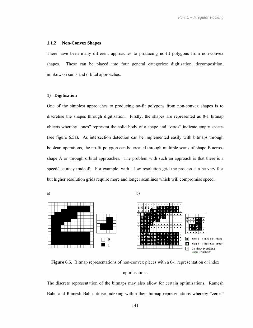
Part C – Irregular Packing
1.1.2 Non-Convex Shapes
There have been many different approaches to producing no-fit polygons from non-convex
shapes. These can be placed into four general categories: digitisation, decomposition,
minkowski sums and orbital approaches.
1) Digitisation
O
discretise the shapes through digitisatio shapes are represented as 0-1 bitmap
ne of the simplest approaches to producing no-fit polygons from non-convex shapes is to
n. Firstly, the
objects whereby “ones” represent the solid body of a shape and “zeros” indicate empty spaces
(see figure 6.5a). As intersection detection can be implemented easily with bitmaps through
boolean operations, the no-fit polygon can be created through multiple scans of shape B across
shape A or through orbital approaches. The problem with such an approach is that there is a
speed/accuracy tradeoff. For example, with a low resolution grid the process can be very fast
but higher resolution grids require more and longer scanlines which will compromise speed.
a) b)
Figure 6.5. Bitmap representations of non-convex pieces with a 0-1 representation or index
optimisations
The discrete representation of the bitmaps may also allow for certain optimisations. Ramesh
Babu and Ramesh Babu utilise indexing within their bitmap representations whereby “zeros”
141

Part C – Irregular Packing
and “ones” are replaced with index entries that indicate how many ‘pixels’ must be traversed
horizontally until an empty space is reached [170]. Although they do not calculate no-fit
olygons within their layout generation implementation, it is apparent that the fundamentals of
technique are also applicable to digitised no-fit polygon generation (see
to decompose any non-convex
apes into subpieces that can be ‘managed’ more easily. However, using decomposition
al subpieces and therefore several no-fit polygons must be created. In
subparts or holes are present. For example, Agarwal, Flato and Halperin conduct experiments
p
their indexed scanning
figure 6.5b). Another imaging technique has been used by Crispin et al. for the generation of
leather lay plan layouts within the footwear industry. The no-fit polygon is found using image
processing techniques by filtering an image of the cow hide boundary with an image of the
shape to be placed. The convolution between the two shape images yields the no-fit polygon
(Crispin et al., 2003) [200]. This is another form of the Minkoski sum that is described later.
Ultimately, all digitisation or imaging approaches will result in inaccurate no-fit polygons
because of the loss of information resulting from the discretisation of a continuous space. While
it is true that the resolution could be set to an arbitrarily high value, this may severely affect
computation times. One benefit of the digitisation approach is that it is able to handle most of
the traditional problem cases, such as holes and interlocking concavities. However, one
disadvantage may be that that jigsaw shapes may not fit together after digitisation whereas they
would in their pure vector form.
2) Decomposition
An alternative to the digitisation techniques described above is
sh
usually results in sever
order to conduct intersection testing, the no-fit polygons can remain decomposed or they can be
recombined through union operations. Where possible, a single no-fit polygon offers the fastest
computation time for intersection but will require additional calculations to recombine
constituent parts. This can be computationally expensive and is a difficult undertaking if several
142

Part C – Irregular Packing
on different decomposition and recombination operations with respect to constructing
Minkowski sums of non-convex polygons without holes [244]. They conclude that it is
ounterproductive to use optimal decompositions because the computation times that are
decomposition including
ng. Seidal suggests a fast polygon triangulation algorithm
which only has O(n log n) complexity [247]. Further implementation ails for triangulatio
can be found in Amenta (1997) [248]. However, the triangulation approaches produce more
subpieces than is necessary and ultimately impacts upon computation time within the generation
process. Unlike triangulation, which can be seen as a specialised case of convex partitioning,
generalised convex partitioning algorithms aim to represent polygons with as few convex pieces
as possible. The two key approaches are suboptimal partitioning, which has an O(n) complexity
(Hertel and Mehlhorn, 1983) [249] and optimal partitioning which has an O(n ) complexity
(Chazelle and Dobkin, 1985) [250]. Agarwal, Flato and Halperin (2002) state that it is generally
c
required to calculate them outweigh the benefits achieved during recombination. The authors
report that the recombination operations are the most costly and give example execution times
that range from a few seconds to produce the no-fit polygon for shapes involving a small amount
of concavities up to twenty minutes for highly irregular shapes.
a) Convex Pieces
It was already discussed that no-fit polygon generation is trivial when convex shapes are
involved. If shapes with concavities can be divided into convex pieces, the fast convex no-fit
polygon generation techniques can be employed. The simplification of geometrical intersection
through the decomposition of non-convex shapes to convex pieces was suggested and discussed
in Avnaim and Boissonnat (1987) [245] and Cuninghame-Green and Davis (1992) [246]. The
main difficulties with such an approach are the decomposition and recombination algorithms.
There are many well-known approaches that can be used for
triangulation and convex partitioni
det n
3
143

Part C – Irregular Packing
more efficient to use suboptimal partition algorithms because of the computational overhead
inherent with optimal partitioning but they also suggest that an alternative and possibly more
efficient approach is to perform convex covering instead [244]. Some possible decompositions
of an irregular polygon into convex pieces are shown in figure 6.6.
a) b) c) d)
Figure 6.6. Convex Decompositions: a) irregular polygon, b) triangulation, c) convex division
(vertex to vertex), d) convex division (vertex to edge)
Once irregular polygons have been decomposed into convex pieces, the no-fit polygon may be
generated by recombining the no-fit polygons produced by passing each convex piece of shape
B around each convex piece of shape A. Providing these no-fit regions have been generated in
relation to a reference point, they may then be recombined. The disadvantage with this
approach is that recombination can be difficult because the no-fit polygons of the convex
ay cross and, therefore, care must be taken when constructing the no-fit polygon
entity. Particular difficulty occurs if the original shapes contain holes as it is unclear whether
intersecting no-fit polygon subsections define holes or whether they define regions that may be
discarded.
b) Star-Sha
partitions m
ped Polygons
144

Part C – Irregular Packing
Li and Milenkovic decompose shapes into convex and star-shaped polygons. A star-shaped
polygon has the property that there exists at least one internal point, or ‘kernel point’, that can
see the entirety of the polygon (Preparata and Shamos, 1985 [235]; O’Rourke, 1998 [236]).
Figure 6.7 shows one non-star-shaped polygon and one star-shaped polygon. By extending the
concavity edges and elimination of invisible regions it is evident that the star-shaped polygon
has a region, Rkernel, that is defined within which a kernel point can be placed to see the entire
olygon boundary. Conversely, this is not the case with the non-star-shaped polygon because no
gion can be defined in which to place a kernel. Thus, star-shaped polygons are situated
convex and non-convex shapes in terms of generality.
p
re
somewhere between
Figure 6.7. a) Non-star-shaped polygon, b) Star-shaped polygon
The authors state that star-shaped polygons are ‘closed’ under Minkowski sum operations and
rovide a proof that the Minkowski sum of two star-shaped polygons also yields a star-shaped
vic, 1995) [69]. The no-fit polygon is then created through use of an
) Phi-Functions
p
polygon (Li and Milenko
angular sweep line algorithm. The authors do not state whether they recombine the no-fit
polygon regions into one no-fit polygon entity or whether they perform multiple no-fit polygon
intersection tests during the layout generation stage.
c
145

Part C – Irregular Packing
An alternative approach is presented by Stoyan and is based on the use of “phi-functions”
(Stoyan, Novozhilova and Kartashov, 1996) [251]. Phi-functions define mathematical
intersection relationships between pairs of standard or “primary” objects such as rectangles,
circles and convex polygons (Stoyan et al., 2001) [252]. The authors further develop their work
to enable the definition of mathematical intersection relationships for non-convex polygons
through the union, intersection and complement of primary objects (Stoyan et al., 2002) [253].
The resultant intersection test between two shapes during layout generation is performed
through comparisons of phi-functions between all pairs of the primary objects that define shape
A and shape B.
3) Minkowski Sums
The no-fit polygon construct can be unified through the use of Minkoski sums (a form of vector
addition) and was first suggested by (Stoyan and Ponomarenko, 1977) [238]. The concept is as
follows: given two arbitrary point sets, A and B, the Minkowski sum of A and B is defined by
the following:
A ⊕ B = {a + b: a ∈ A, b ∈ B}
In order to produce no-fit polygons the Minkowski difference can be used, A ⊕ −B,. This is
equivalent to the two input polygons in opposing orientations and is easily shown through
simple vector algebra (Bennell, Dowsland and Dowsland, 2001) [239]. We can verify that this
is the case using the simple convex only case (section 2.3.1) whereby we place shape A in its
anticlockwise orientation and shape B in its clockwise orientation. We can state that the method
of Cuninghame-Green [237], involving convex shapes only, is also using the Minkowski
difference in its most basic form.
146

Part C – Irregular Packing
Whilst non-mathematical implementation details of such approaches are scarce, Ghosh and
Bennell provide excellent explanations and implementation details for no-fit region calculation.
As such, their contributions are briefly summarised. Ghosh details the production of no-fit
polygons through the notion of Minkowski difference and demonstrates a simple extension to
the convex only case that allows for the generation of no-fit polygons for non-convex shapes.
The drawback is that this approach will only work providing that the concavities of the two
shapes do not interfere or interlock (Ghosh, 1991 [254]; Ghosh, 1993 [255]). Where this is not
the case, a modification is proposed but is only outlined briefly. Bennell, Dowsland and
Dowsland (2001) state that Ghosh’s modification would cause a “cumbersome tangle of
intersecting edges” which would be difficult to recombine to form the no-fit polygon [239].
They introduce a further implementation that reduces the amount of tangled edges and give
thorough implementation details and pseudocode of the entire process. They also report fast
generation times of around 0.3 seconds for each of five separate datasets from the literature.
However, they state that their approach cannot deal with internal holes as it is difficult to detect
which of the internal no-fit polygon edges can be discarded and which form the internal no-fit
regions. In chapter eight the robustness and speed of a new orbital approach is compared
through the reporting of generation times for 32 datasets of the literature some of which include
holes.
4) Orbital Sliding Approach
The orbital sliding approach is the main focus of chapter eight whereby a new approach is
presented based on the physical sliding of one polygon around another using standard
trigonometry. The no-fit polygon is defined by tracing the motion of a locus point of the sliding
polygon when orbiting. The first discussion and implementation of an orbiting approach for the
generation of ‘envelopes’ is detailed in Mahadevan (1984) [256] and is further investigated by
Kendall (2000) [8]. The key elements of Mahadevan’s approach are: calculation of touching
147

Part C – Irregular Packing
vertices and edges, determination of the translation vector and calculation of the translation
length. The calculation of intersecting edges is performed using the notion of D-functions which
ere introduced by Konopasek in 1981 [146]. Mahadevan modifies the D-function test to also
ed to calculate the translation distance. It
is also important to project the translation vector in the reverse direction of the stationary
polygon. The orbiting shape is then translated along the translation vector by the smallest
distance (from projection and intersection tests). This ensures the two polygons never intersect
but always touch. The process continues until the orbiting polygon returns to its original starting
position. A more detailed description of Mahadevan’s approach is deferred because many of its
features are also used within the newly proposed orbital approach which is described in chapter
eight (where applicable, Mahadevan’s approach is compared and improvements of the new
approach are stated). The major disadvantage with Mahadevan’s algorithm is that it cannot
generate the full no-fit polygon for shapes involving holes or some concavities. The problem
occurs when the orbiting polygon can be placed inside a concavity of the stationary polygon but
the concavity has a narrow entrance. In this case the orbiting polygon is too wide and will
simply slide over the concavity. Oliveria, Gomes and Ferreira also use Mahadevan’s
implementation within their work on irregular packing and include steps to detect such problems
(Oliveria, Gomes and Ferreira, 1996) [257].
This chapter provided a brief review of geometric considerations for automated packing and a
summary of the different approaches that have been used for the generation of no-fit polygons.
In chapter eight, a new orbital no-fit polygon procedure is described and is shown to be able to
handle all of the known classes of degenerate shapes.
w
calculate touching points which is a necessity for both Mahadevan’s algorithm and the new
approach presented in chapter eight. This information is then used to select a translation vector
based on the touching edge. The translation vector is then projected through each vertex of the
orbiting shape and then intersecting edge testing is us
148

Part C – Irregular Packing
CHAPTER SEVEN
Automated Packing using
Trigonometric Approaches
This chapter presents a method for irregular packing using an improved bottom-left fill strategy
through the use of new shape primitive overlap resolution techniques. These techniques
efficiently deal with the irregular nature of shapes in order to produce high quality solutions in
quick time. Furthermore, the proposed approach allows problems containing shapes consisting
of circular arcs and holes to be nested. In the vast majority of the irregular packing literature
(discussed in section 2.3), there have only been approaches that can handle circular arcs by using
line approximations. By combining the new techniques with both hill climbing and tabu local
search methods the proposed irregular packing approach has been tested using the 26 existing
problems from the literature (as discussed in section 2.3.2). Also introduced are 10 new
irregular benchmark problems that have been produced from industrial style shapes, five of
which contain circular arcs and three which include holes.
7.1 Motivation for the Approach
There have been many different approaches for producing solutions for the irregular two-
dimensional stock cutting problem. It should be noted that, in general, the approaches that have
achieved the best known results have used a no-fit polygon based technique to generate potential
placement positions and/or test for overlaps [172]. While the no-fit polygon is a powerful
geometric technique, there are several issues that make it limited in scalability for industrial
149

Part C – Irregular Packing
applications. No-fit polygon techniques are notorious for the large number of degenerate cases
that must be handled in order to be completely robust (as discussed in section 6.6). A further
problem with no-fit polygon generation techniques is that, as far as the author is aware, there has
previously been no algorithm that successfully handles true arc geometry.
As the previous no-fit polygon based packing techniques are unable to handle arcs, most
methods and test problems approximate arcs using a sequence of lines. The problem with
approximations is that there is an accuracy to time trade-off. That is to say, that if we model the
arc with fewer lines then the accuracy of the approximation is reduced but the shape is less
complex and if we increase the quantity of lines then accuracy is improved but the resultant
shape is made more complex. When performing translation or rotation operations, obviously
shapes with a larger number of lines will take longer to manipulate than a shape with fewer lines.
Ultimately, there will always be inaccuracy when modelling arcs as a series of lines and in
adding more lines to approximations, operating on that approximation required greater time.
The geometry implementation that has been developed is able to model shapes composed of both
lines and non-approximated arcs and is able to conduct fast shape intersection operations to an
accuracy of 10-9 metres. The development of such a geometry system is a complex and time-
consuming undertaking and the author would like to suggest that other practitioners may like to
consider general geometry libraries such as LEDA and CGAL (as discussed in section 6.1).
Note: a new no-fit polygon algorithm that is able to cope with such degeneracies is developed in
chapter eight but this had not been attempted until the latter stages of this research and,
therefore, was not available during the development for the approach in this chapter.
150

Part C – Irregular Packing
In real world industrial settings, and especially for profiling (sheet metal cutting) within the steel
cutting industry, it is imperative that automated packing approaches are able to handle arcs,
concavities and holes. These requirements mean that the no-fit polygon techniques that have
previously been discussed are not currently suitable. Traditionally, industry has used a bottom-
left-fill approach based on an iterative grid approximation in which arcs are represented by
approximated lines. The grid approach aims to reduce the infinite number of potential positions
(due to the continuous nature of space) to a fixed set of potential locations. The algorithm works
as follows: when placing a shape on the sheet the algorithm places the shape in the first grid
location (bottom-left point) and then checks for intersection with shapes already assigned to the
sheet. If there are no intersecting shapes then the shape is assigned to the sheet in its current
position and a new shape is packed starting from the first grid location. However, if the current
shape does intersect with another shape on the sheet then it is moved to the next grid position
and is tested for intersection again, continuing the process until a valid position is found. This
means that using a lower resolution grid will, in the general case, adversely affect the quality of
the solution because shapes are placed in later positions than they could otherwise be placed if a
higher resolution grid was used. This causes, as is often found in cutting and packing, an
accuracy to time trade-off.
Figure 7.1. a) low resolution grid approach b) high resolution grid approach c) variable shift
approach
151

Part C – Irregular Packing
Figure 7.1 shows the potential locations for two iterative grid approaches with differing
resolutions and also the proposed overlap resolution method. The packing method involves
placing shapes leftmost (and then bottommost) within the sheet. Therefore, in the two iterative
grid approaches, the first location tried is the bottom-left grid location and then the grid location
above it and so on until the shape is placed or moves off the top of the sheet. After moving off
the top of the sheet, the shape is relocated at the bottom of the next column of grid points and the
process continues. Therefore, with the grid approaches, there are a finite number of locations for
which shapes may be placed. The iterative grid approach of figure 7.1b has a higher resolution
than that in figure 7.1a and therefore has more potential placement locations and should result in
ore compact packings although this will require longer computation times as each shape must
e tried in many more potential positions than in figure 7.1a. The proposed variable shift
od and the proposed approach follow a similar
conceptual procedure when placing shapes, the proposed approach has both a faster and more
accurate method of producing solutions. For irregular packing, it is convention to minimise
horizontal length rather than height (as in rectangle packing), but as the two are conceptually
identical, the recognised convention will be used.
m
b
approach is shown in figure 7.1c and has an infinite number of potential locations due to its
continuous y axis property and therefore can produce more compact packings.
The approach that is described in the next section, unlike the iterative grid approach, is not
restricted to moving shapes by a fixed translation when intersecting with another shape. This is
achieved by using the underlying geometric primitives of intersecting shapes to resolve the
overlap. This has two main advantages in that intersecting shapes can be resolved so that they
touch exactly and, secondly, that this accuracy is achieved in a smaller number of steps than the
iterative grid mechanism. Although the grid meth
152

Part C – Irregular Packing
7.2 The New Bottom-Left-Fill Approach
In this section, the techniques used to resolve overlap are explained. The overall algorithm
pseudocode can be found in section 7.2.4.
7.2.1 Geometrical Definitions
In order to illustrate the new packing method the terms “primitive”, “loop” and “shape” are
defined. For the purposes of this discussion, a “primitive” is defined as either an arc or a line. A
line is represented by its start and end points whereas an arc is circular and is represented
through a centre point, radius, start angle and offset angle. A “loop” is defined as an anti-
clockwise closed list of primitives where each primitive’s end point is the start point of the next
primitive. Non-simple polygons are not allowed (essentially these are polygons where the edges
are allowed to intersect one another) as we are only interested in shapes that can be physically
cut from a material (O’Rourke, 1998) [236]. A “shape” is defined as one outer loop and 0….n
internal loops which can be thought of as holes in the shape. Figure 7.2 shows an example shape
where the solid line is used to represent the outer loop and dashed lines the holes (internal
loops).
Figure 7.2. Shape containing holes
153
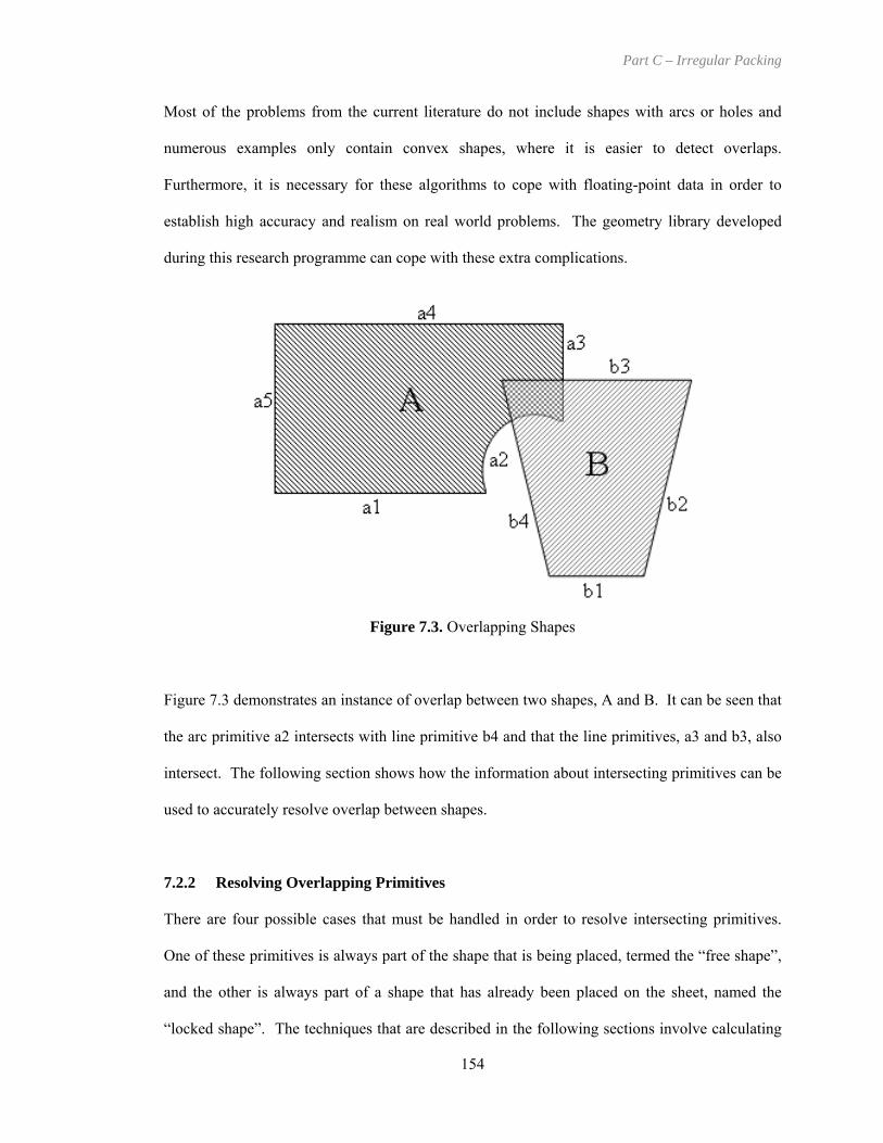
Part C – Irregular Packing
Most of the problems from the current literature do not include shapes with arcs or holes and
numerous examples only contain convex shapes, where it is easier to detect overlaps.
Furthermore, it is necessary for these algorithms to cope with floating-point data in order to
establish high accuracy and realism on real world problems. The geometry library developed
during this research programme can cope with these extra complications.
Figure 7.3. Overlapping Shapes
Figure 7.3 demonstrates an instance of overlap between two shapes, A and B. It can be seen that
the arc primitive a2 intersects with line primitive b4 and that the line primitives, a3 and b3, also
intersect. The following section shows how the information about intersecting primitives can be
used to accurately resolve overlap between shapes.
7.2.2 Resolving Overlapping Primitives
There are four possible cases that must be handled in order to resolve intersecting primitives.
One of these primitives is always part of the shape that is being placed, termed the “free shape”,
and the other is always part of a shape that has already been placed on the sheet, named the
“locked shape”. The techniques that are described in the following sections involve calculating
154

Part C – Irregular Packing
the positive e required t shape such tha primitives no
longer solv he two intersecting primitives, the
two shapes may resolved in other primitives belonging to the shapes may
also intersect or the free shape may be ent ed shape (discussed in
section 7.2.3). However, repeated applic of these techniques ways resolve
overlapping shapes with the ired. Table 7.1 shows the
ases that must be handled and the subsections in which the resolution method is discussed.
Intersecting Primitive Intersecting Primitive
vertical distanc
intersect. Whilst this re
o translate the free
es the overlap between t
t the two
still not be fully that
irely contained in the lock
ation will al
smallest positive vertical distance requ
c
Free Shape’s Locked Shape’s Section
Line Line 7.2.2.1
Line Arc 7.2.2.2
Arc Line 7.2.2.3
Arc Arc 7.2.2.4
Table 7.1. Possible intersection types
It should be noted that throughout all of the cases, the locked shape’s intersecting primitive,
which is called the “locked primitive”, is a primitive belonging to a shape that has already been
assigned to the sheet and its position may not change whereas the intersecting primitive,
belonging to free shape, is termed the “free primitive”. An explanation of the steps required in
resolving the intersections of these cases is provided but firstly some terminology is introduced.
The “x span” of a primitive can be thought of as the horizontal span of its bounding rectangle.
Figure 7.4 highlights the x spans for both primitive types. Another concept used is that of an
“infinite vertical line”. This is a vertical line that spans from negative infinity to positive infinity
congruent to the y axis. The notations that are used in the d and descriptions of the
following subsections are presen
iagrams
ted in table 7.2.
155

Part C – Irregular Packing
x span
x spa
Figure 7.4. Line and arc x spans
Symbol
Description
A1 A2 Primitive A (the free primitive). A1, A2 Start point (A1) and end point (A2) of primitive A B1 B2 B1, B2
Primitive B (the locked primitive). Start point (B1) and end point (B2) of primitive B
CP Centre point of an arc primitive c1…cn Intersection points t1, t2 Tangent points of a line on an arc Infinite vertical line
(short-dashed vertical line)
Perpendicular to a line primitive (long-dashed line)
Translation used to resolve overlap (bolded vertical arrow)
Table 7.2. Notation for diagrams and descriptions
n
Having established the required terminology and notation, each case is explained as outlined in
table 7.1.
7.2.2.1 Line & Line (Free Line moving through Locked Line)
In order to resolve any two intersecting lines we find the end points of each line, A and B, that
are within the x span of the other, these points are known as the points in range (pir). An infinite
vertical line is passed intersection points through each of the pir originating from line A and the
156

Part C – Irregular Packing
of these lines with line B are found. The distance is calculated for each pir from line A and its
corresponding intersection point on line B by using formula (1).
Infinite vertical lines are also passed through each of the pir originating from line B to find their
intersection points with line A. A different formula, formula (2), is used to calculate the
distances when the pir originates from the locked
distancePirA = intersectionPointB.y - pirA.y (1)
primitive (line B).
distancePirB = pirB.y - intersectionPointA.y (2)
For the resolution method, the overlap must always be resolved by translating line A in the
positive vertical direction. The distance formulae, given in formulas (1) & (2), may yield
negative results and, therefore, such results are not valid positive vertical movements and can be
eliminated. These distance formulae also form part of the strategy for resolving the other
intersection cases. Fo lt which can be used
vertically translate line A in order to fully resolve the intersection between the lines. An
r two lines, there always exists one valid positive resu
to
example of this approach is shown in figure 7.5.
A1 (pirA)
A2
B2 (pirB)
c1
c2
B1
A1 (pirA)
A2
B2 (pirB)
B1
A1
A2
B1
B2
(a) (b) (c)
itivesFigure 7.5. Resolution of intersecting line prim
157

Part C – Irregular Packing
Here, point A1 is within the x span of B1 B2 and B2 is within the x span of A1 A2. Let
these points be labelled pirA and pirB respectively (see figure 7.5a). An infinite vertical line is
passed through pirA to create intersection point c1 and another through pirB to create
intersection point c2 (shown in figure 7.5b). The distance between pirA and c1 is calculated
sing formula (1) and the distance between pirB and c2 is calculated using formula (2). In this
cond is negative. Formula (3)
yTranslation = max(c1.y - pirA.y , pirB.y - c2.y) (3)
The result of formula (3) is shown pictorially as the bolded arrow in figure 7.5b. Figure 7.5c
shows how the overlap has been resolved by vertically translating line A by this positive
translation. In practice, all of the primitives of shape A are translated vertically by this positive
distance, not just the line involved in the overlap.
7.2.2.2 Line & Arc (Free Line moving through Locked Arc)
In this case, where a line is intersecting with an arc, the positive vertical translation must be
found with which the line should be translated in order to completely resolve its intersection
with the arc. As with the Line & Line case (section 7.2.2.1), the points in range of each
primitive can be utilised. However, because an arc is involved, the use tangent points between
the arc and line primitives may be required. Figure 7.6 shows an example where applying the
points in range method alone is not sufficient to resolve the overlap.
u
example, the first distance yields a positive result whilst the se
shows how the distance formulae (1) & (2) may be combined into a “max” function call:
158
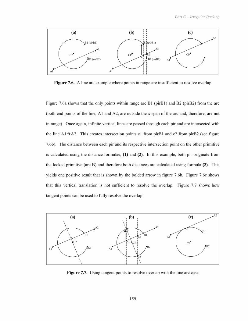
Part C – Irregular Packing
B2 (pirB2)B2 (pirB2)
B1 (pirB1)
CP
B1 (pirB1)
CP c1c2 CP
(a) (b) (c)
A1
A2
A1
A2
A1
A2
Figure 7.6. A line arc example where points in range are insufficient to resolve overlap
Figure 7.6a shows that the only points within range are B1 (pirB1) and B2 (pirB2) from the arc
(both end points of the line, A1 and A2, are outside the x span of the arc and, therefore, are not
in range). Once again, infinite vertical lines are passed through each pir and are intersected with
the line A1 A2. This creates intersection points c1 from pirB1 and c2 from pirB2 (see figure
7.6b). The distance between each pir and its respective intersection point on the other primitive
is calculated using the distance formulae, (1) and (2). In this example, both pir originate from
the locked primitive (arc B) and therefore both distances are calculated using formula (2). This
yields one positive result that is shown by the bolded arrow in figure 7.6b. Figure 7.6c shows
that this vertical translation is not sufficient to resolve the overlap. Figure 7.7 shows how
tangent points can be used to fully resolve the overlap.
B2
B1
CP B2
B1
CP CP
(a) (b) (c)
A1
A2
A1
A2
A1
A2
t1
c1
B2
B1 t1
t2
c2
Figure 7.7. Using tangent points to resolve overlap with the line arc case
159

Part C – Irregular Packing
The tangent points can be found by translating the perpendicular (or “normal”) of the line such
that it passes through the centre point of the arc, CP, as shown in figure 7.7a. The intersection of
the perpendicular with the arc gives the tangent points, t1 and t2 (see figure 7.7b). These tangent
oints are then used in a similar manner to the point in range technique whereby infinite vertical
line A1 A2 to give points c1
tion whereas t2 would give a
egative translation distance. Therefore, translating the line A1 A2 by the distance given by
e calculation: t1 - c1 will resolve the overlap (see figure 7.7c). It should be noted that if the
intersection of the perpendicular line with the arc yields no tangent points or the tangent points
result in negative translation distances using formula (4) then the point in range technique must
be able to resolve the overlapping primitives.
7.2.2.3 Arc & Line (Free Arc moving through Locked Line)
This case, where there is a free arc through a locked line, involves a similar approach to the free
line & and,
erefore, will not be repeated here. However, because the arc is now the free primitive (arc
p
lines are passed through each tangent point and intersected with
and c2. The translation distances can then be calculated by substituting each tangent point, t1
and t2, for pirB into formula (2). This gives formula (4).
distanceTangentB = tangentB.y - intersectionPointA.y (4)
In the example, it can be seen that t1 would yield a positive transla
n
th
locked arc case. Once again, the same technique for points in range applies
th
A1 A2) and the line is now the locked primitive (line B1 B2), we must substitute calculated
tangent points and their intersections into formula (1) instead of formula (2) (as was the previous
case in section 7.2.2.2). An example of this is shown in figure 7.8.
160

Part C – Irregular Packing
(a) (b)
A2 (pirA)
A1 CP
B1 (pirB)
B2
A2
A1CP
B1
B2
t1
(c) A2
A1 CP
B2
t1 c1
B1
Figure 7.8. Resolving overlap using the tangent point method with the arc line case
Figure 7.8a shows that points A2 and B1 are the points in range, pirA and pirB. However, both
of the pir produce negative translations (using formulae (1) and (2)) thus they cannot be used to
od must be used again. In the
.y (5)
Using formula (5) with the example yields a positive translation distance as shown by the bolded
arrow in figure 7.8b. The intersection is resolved by translating the arc, A1 A2, by this vertical
distance as shown in figure 7.8c. If the tangent point method does not find any tangent points or
no positive translation is found then the points in range method can fully resolve the intersection.
7.2.2.4 Arc & Arc (Free Arc moving through Locked Arc)
The arc through arc case initially uses the point in range technique. This will not be repeated in
detail here as it of the method
resolve the intersection). Therefore, the tangent points meth
example, only one tangent point is found because the perpendicular line intersects the arc in only
one place. Figure 7.8b shows that an infinite vertical line is passed through the tangent point, t1,
and is intersected with line B1 B2 to produce point c1. The translation distances can then be
calculated by substituting tangent points for pirA in formula (1). This gives formula (5).
distanceTangentA = intersectionPointB.y - tangentA
is used throughout the previous cases. However, a brief example
161

Part C – Irregular Packing
is shown in figure 7.9. Figure 7.9a shows the points in range, figure 7.9b shows the infinite line
intersections passing through the pir
7.9c shows the resolved overlap after translati e result of the distance formulae.
to create the intersection points, c1, c2 and c3, and figure
ng arc A by th
An example of arcs of opposite orientations is shown in figure 7.10.
CPb
A1
B1 (pirB1) B2 (pirB2)
CPa
CPb
A1 A2 (pirA2)
B1 (pirB1) B2 (pirB2)
CPa
A2 (pirA2)
c3c2
c1
Pb
C
A1
B1 B2
CPa
A2
(c) (a) (b)
Figure 7.9. Resolving arc intersections using the points in range
A1 ( ) ( )
aFigure 7.10. Using the Pythagorean theor
CPa
B1
B2
A1
A2
CPb dx
dy h
16
b
em to resolve arc intersections (method 1)
B1
B2
CPb dx
dy′h′
CPa
A2
2

Part C – Irregular Packing
For the situation of figure 7.10, where the point in range method is unable to resolve the
intersection between the two arc primitives, we use two circle tangent methods that utilise the
radii of the arcs and the Pythagorean theorem.
Given that rA is the radius of the free arc A1 A2 and rB is the radius of the locked arc B1 B2
we can make the following observations:
From figure 7.10a, when the arcs are intersecting: (rB – rA) < h < (rA + rB)
Therefore:
yTranslation = (dy′ - dy) : where dy′ = sqrt((h′ * h′) – (dx * dx)) (6)
This inte
A further arc through arc case that can occur involves two arcs of similar orientation as shown in
figure 7.11.
From figure 7.10b, when the intersection has been resolved: h′ = (rA + rB)
rsection can then be resolved by translating arc A by the result of formula (6).
B1B2
A1 A2
dx
dy h
CPa
CPb B1B2
A1 A2
dx
dy′ h′
(a) (b)
CPa
CPb
Figure 7.11. Using the Pythagorean theorem to resolve arc intersections (method 2)
163

Part C – Irregular Packing
Given that rA is the radius of the free arc A1 A2 and rB is the radius of the locked arc B1 B2,
the following observations can be made:
Therefore, the translation distance can be calculated by formula (7).
yTranslation = (dy – dy′) : where dy′ = sqrt((h′ * h′) – (dx * dx)) (7)
If the result of formula (7) is positive, applying this vertical translation to arc A will resolve the
overlap. It can be seen that, whereas the first circle tangent resolution method translates the free
arc to the exterior of the locke
From figure 7.11a, when the arcs are intersecting: (rB – rA) < h < (rA + rB)
From figure 7.11b, when the intersection has been resolved: h′ = (rB - rA)
d arc circle, the second method translates the free arc to be inside
f the arc circle. This is important for the correct manipulation of both convex and concave arcs.
icular of the line primitive is
isplaced through the arc’s centre point and is intersected with the arc to find tangent points.
d the line is the “free primitive” formula (4) is used to
circle tangent methods that can resolve intersections. The first method is calculated using
formula (6) and results in t rate. The sec method
o
7.2.2.5 Intersection Resolution Summary
The four possible intersection cases that may occur within intersecting shapes have been
described. It has been shown that each case may be resolved by using the points-in-range
method by using formulae (1) and (2). This will always resolve the intersection where two lines
are involved (see formula (3)). If arcs are involved, the point in range method may not be
sufficient to resolve intersections fully and other supplementary tangent based techniques may
be required. When an arc and line are intersecting, the perpend
d
Where the arc is the “locked primitive” an
calculate the vertical translation required. Formula (5) is utilised when the arc is the “free
primitive” and the line is locked. The final case, where two arcs are intersecting, introduced two
he respective arc’s p nt circles being sepaare ond
164

Part C – Irregular Packing
results in the respective free arc’s parent circle being contained by the locked arc’s parent circle
in the
plementation) whereby it is preferred to resolve line only cases if many intersecting pairs of
p
an the iterative grid method outlined in section 3.2. One further circumstance is the
ble that a shape may become entirely contained within other
already assigned shapes, as shown in figure 7.12.
(and is given in formula (7)).
It is of note that the most simple of the cases is where two lines are involved, as no extra tangent
calculations are required. This presents optimisation possibilities (which are included
im
rimitives between two shapes exist. Although repeated applications of these techniques may be
necessary to fully resolve the overlap between two shapes, this is more efficient and accurate
th
overlapping case in which one shape is completely contained within another. This requires
another resolution strategy as there are no intersecting primitives.
7.2.3 Dealing with Contained Shapes
During the nesting process it is possi
B
A
B
A
lpA
c1
c2
c3
c4
Figure 7.12. Resolving a contained shape
Here there are no intersecting primitives to resolve so another approach is required. As the free
shape A is contained by locked shape B the lowest point on shape A is used, lpA, through which
165

Part C – Irregular Packing
an infinite vertical line is passed. The resultant intersection of the infinite vertical line and shape
B gives the points c1 … cn. The translation that is performed is defined by formula (8):
yTranslation = min(c1.y – lpA.y, … cn.y – lpA.y) : where (ci.y – lpA.y) > 0, i = 1... n (8)
igure 7.13 shows an instance where employing this technique does not fully resolve overlap
there are
scribed for
employed. This process continues until the shape
tion is completely resolved.
resolving shape intersections, the vertical translations may cause the free shape to intersect
other already assigned shapes. These intersections must also be resolved until the shape
does not intersect and can be assigned to the sheet or until the shape has moved off the top of the
sheet. In the latter case, the shape must be translated back to the bottom of the sheet and the
shape’s x location is incremented and the process resumes until all shapes are placed.
In the example, the value for vertical translation would be c2.y – lpA.y.
F
between the shapes. However, shape A is no longer contained by shape B and
intersecting primitives once more. This allows the techniques that have been de
resolving primitive intersection to be
intersec
Figure 7.13. Contained shape and overlap is not fully resolved
In
with
B
A
c4
B
c3
Ac2
lpA
c1
166

Part C – Irregular Packing
7.2.4 Summary – The Bottom-Left-Fill Algorithm
Given the functionality outlined in the previous sections the bottom-left-fill process can be
describes using the following pseudo code:
Input Sequence : shapes[1..m][1..n] where m = number of different shapes, n = number of rotations for given shape[m] sheetshape[1..q] where array holds placed shapes on the sheet
x = current x position resolution = x increment step value
Begin
Place shapes[1][1] at bottom left of sheet (0,0); Add shapes[1][1] to sheetshape[1..q]; for (i = 2; i <= m; i++) { for (j = 1; j <= n; j++) {
while (Overlap(shapes[i][j], sheetshape[1..q]))
Get Intersecting Primitives of shape[i][j] and sheetshape[1..q];
if (shapes[i][j] off top of sheet) { x = x + resolution; place shape[i][j] at (x,0); }
positions[1..n] first available position for rotation of shape shapes[][1..n]
place shapes[i][j] at bottom left of sheet;
{
Resolve Overlapping primitives;
}
Add shapes[i][j]'s coordinate to positions[1..n]; }
Add shapes[i][1..j] with leftmost position[1..n] to sheetshape[1..q] }
This bottom-left-fill placement algorithm takes a sheet size and an input sequence of shapes and
their allowable rotations. The algorithm starts by placing the first shape in the lower left corner
of the sheet in its most efficient orientation. The most efficient orientation is the rotation which
yields the smallest bounding width for the shape, with equal widths being resolved by the
Return Evaluation (total length of packing); End
167

Part C – Irregular Packing
rotation that faces concavities to the right. This enables later shapes to easily be placed within
ther already placed
apes and the shape is within the remits of the sheet, then the location of the shape is valid and
solution).
the concavity regions. With subsequent shapes, if a copy of this shape has not been placed on
the sheet, the shape starts at the lower left corner of the sheet. If a copy of the shape has
previously been assigned to the sheet, then the new copy starts from where the previous copy of
the shape was placed. A valid location for placement is found by testing for intersections and
containment. If the shape is not intersecting or contained by (or containing) o
sh
therefore can be assigned to the sheet. When a shape is in a position that intersects with already
assigned shapes, the resolution techniques (described earlier in this section) are used to resolve
the overlap in a positive vertical direction (upwards congruent to the y axis of the sheet). If
resolving overlap results in the shape moving off the top of the sheet, then it is returned to the
bottom of the sheet and incremented along the positive x axis by a certain value (known as the
re
The process continues as before with overlap/intersection testing and resolution of the
intersections until the shape can be placed. Packing is completed when all shapes have been
assigned to the sheet and the solution can be returned to the user. Shapes are always packed in
the order they appear in the input sequence that is provided by the local search techniques.
168

Part C – Irregular Packing
7.2.5 Local Search
It is usual to apply some sorting criteria to the shapes of a given problem before packing, often
by decreasing length or area. Although these often yield solutions of reasonable quality, further
improvements can be found if a local search mechanism is applied to generate new input
orderings. This approach has been used during the experiments of section 7.4 by applying hill
climbing and tabu search for both area and length pre-sorted arrangements.
A standard hill climbing algorithm is used during the experiments which simply applies
erators to the current solution in order to find a neighbour of increased quality. If an improved
neig u bour
no provement on the current solution it is discarded and the search continues with other
neighbours. The best solution is returned at the end of the search.
The hanism implemented for the experiments is similar in nature to that
described in Glover (1993) [
s and the cycle continues. The use of a tabu list means that
ut this chapter,
size of 5 solutions and a tabu list length of 200 solutions are used. These
lu ere chosen from a set of possible values during initial experimentation.
The perators used throughout both search techniques are 1 Opt, 2 Opt, 3 Opt, 4 Opt and N Opt.
1 Opt removes a randomly chosen shape and inserts it at a random location in the sequence. 2
Opt swaps two randomly chosen shapes in the order, although not two of the same type as this
would produce the same result, this is extended up to 4 Opt where four randomly selected shapes
are swapped. N Opt selects a random number of shapes to swap and is likely to produce a
op
hbour is fo nd it is adopted as the current solution and the search continues. If the neigh
is t an im
tabu search mec
258]. The process generates a given number of neighbours and
moves to the best solution in this subset of the neighbourhood. This solution is then used to
g the next set of neighbourenerate
recently seen solutions, within a given list length, will not be revisited. Througho
a neighbourhood
va es w
o
169

Part C – Irregular Packing
radically different solution, and thus diversify the search. The solution operator is chosen by
pared to a weighted scale, which gives the particular
oblem Sha Quantiti e Rota Sheet Sirrent.ord g = Sort sing a ecreasing th)
Beg
cur ation = B m-Left-F ring)best = current; while (!Stopping Criteria) // either max number of iterations or time based { ct Operat 1,2,3,4, for (i = 0; i < {
neighbour[i].ordering = Generate NotTabu Neighbour(current ordering, opt); Bottom-Left-Fill(neighbour[i].ordering);
{
if (neighbour.evaluation <= current.evaluation) { current = neighbour; }
if (current.evaluation < best.evaluation) { best = current; }
return best;
means of a random number that is then com
operator to be used. Each operator has a different chance of selection, from 1 Opt which has the
largest chance of being selected down to N Opt which has a much lower chance of being
selected. This is because the less radical operators allow for concentration of the search and the
highly radical operators, e.g. N Opt, enable the search to escape local optima. The following
pseudocode shows how both of the local searches interface with bottom-left-fill:
INPUT: Pr pes, es and Allowabl tions, ze cu erin Ordering(decrea rea, d leng
in
rent.evalu otto ill(current.orde ;
opt = Sele or ( n Opt);
if (TABU) {
neighbourhood size; i++)
neighbour[i].evaluation = } current = GetBestNeighbour(neighbour[]); } else if (HILL CLIMBING)
neighbour.ordering = Generate Neighbour(current.ordering, opt); neighbour.evaluation = Bottom-Left-Fill(neighbour.ordering);
}
}
End
170

Part C – Irregular Packing
7.3 Benchmark Problems
In order to compare the proposed algorithm with the current state of the art, the literature
benchmarks are used (see table 2.3). Furthermore, ten new benchmark problems have been
created for the irregular stock cutting problem which include some shapes that are typical of the
metal cutting industry. Table 7.3 gives the details of these new problems including the sheet
width and rotational constraints. The raw data for these instances can be found in appendix D.
Problem Name
Number of Shapes
Rotational Constraints
Sheet Width
Optimal Known
Profiles1 32 90 Incremental 2000 No Profiles2 50 90 Incremental 2500 No Profiles3 46 45 Incremental 2500 No Profiles4 54 90 Incremental 500 No Profiles5 50 15 Incremental 4000 No Profiles6 69 90 Incremental 5000 No Profiles7 9 Yes 90 Incremental 500 Profiles8 Yes 18 90 Incremental 1000 Profiles9 57 90 Incremental 1500 No
Profiles10 91 0 Absolute 3000 No
Table 7.3. New benchmark problems
Line & Arc - Profiles1 to Profiles5
These new problems introduce arcs and holes to the set of benchmark problems. Some of these
shapes, in particular Profiles1 and Profiles2, have been chosen from a library of standard shapes
within the sheet metal profiling industry. All of these problems contain at least one shape
consisting of one or more arcs. For these problems the optimal solutions are not known.
L
A further five problems have be y non-arc implementations (but
also include shapes with holes). Once again al solutions are not known with the
rofiles9 is a novelty dataset involving a subset of letters
from the English alphabet. Profiles10 combines polygons from numerous literature benchmarks.
ine Only - Profiles6 to Profiles10
en created which can be tackled b
the optim
exception of Profiles7 and Profiles8 which are ‘jigsaw’ problems where the optimal solutions are
known (1000 units for both problems). P
171
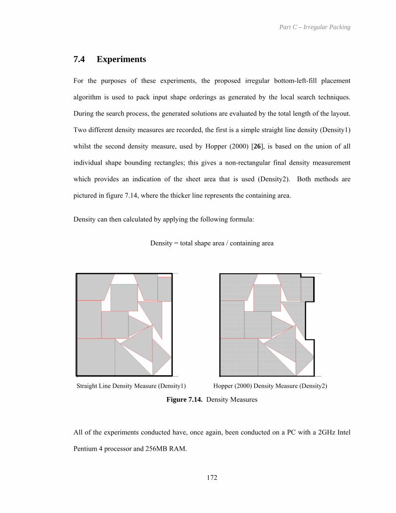
Part C – Irregular Packing
7.4 Experiments
For the purposes of these experiments, the proposed irregular bottom-left-fill placement
algorithm is used to pack input shape orderings as generated by the local search techniques.
During the search process, the generated solutions are evaluated by the total length of the layout.
Two different density measures are recorded, the first is a simple straight line density (Density1)
whilst the second density measure, used by Hopper (2000) [26], is based on the union of all
individual shape bounding rectangles; this gives a non-rectangular final density measurement
which provides an indication of the sheet area that is used (Density2). Both methods are
pictured in figure 7.14, where the thicker line represents the containing area.
Density can then calculated by applying the following formula:
Density = total shape area / containing area
A
P
S
traight Line Density Measure (Density1)Figure 7.14. De
ll of the experiments conducted have, once aga
entium 4 processor and 256MB RAM.
17
Hopper (2000) Density Measure (Density2)
nsity Measures
in, been conducted on a PC with a 2GHz Intel
2

Part C – Irregular Packing
173
7.4.1 Experiments on Literature Benchmark Problems
The literature problems have been divided into two groups, those for which the best known
result is measured using overall nest length and those which have been evaluated using density
measures (see table 2.3 and 2.4). Both the length and density measures are used with all of the
problem instances to facilitate easier comparison with future research. Table 7.4 presents the
results for the length evaluated problems using the tabu and hill climbing search met s
outlined previously (best results shown in bold). Each problem was run 10 times using
iteration runs, for both length and area initial orderings (resulting in a total of 40 runs for each
problem). It seems that tabu search outperforms hill clim ost cases. Table 7.5 shows
the results for the density evaluated problems. In table 7.7, the best results from table 7.4 & 7.5
are shown and include the average times per nest, time taken to find the best solution and the
percentage improvement on the best known result from the literature. For problems where there
has been an improvement upon the best known solution, the percentage is shown in bold
typeface. From these initial experiments, the algorithm proved upon 20 of the
available literature problems. The average overall improvem s is slightly
over 4% and is nearer 6% for the 20 problems where new best solutions have been found.
average the best solutions have been obtained within a few m execution time, although
many of the problems only a few seconds are necessary ance of the
presented algorithm. The average time per nest compares favourably with other literature
approaches utilising the no-fit polygon. For example, Gomes & Oliveira (2002) state that a
layout for the problem SHAPES1 can be generated within 6.18 seconds, on a 450MHz CPU, in
comparison with 0.82 seconds for a solution generated by the proposed automated nesting
approach [172]. The best solution for dataset SWIM was obtained in 607 seconds and is shown
in figure 7.15.
hod
100
26
On
for
bing for m
has im
ent over the 26 problem
inutes
due to the high perform

Le th nsity Dens y21 30 28.72 28 0 5.5% 78.0 8.57i 60 62.57 61 2 2.0% 84.1 2.28
00 33.57 33 0 6.4% 90.1 3.90bs1 20 12.40 12 0 1.7% 89.1 2.02bs2 20 26.40 26 0 4.2% 83.3 6.62ues 60 82.76 81 0 5.4% 88.6 1.97
1A 70 14.73 14 7 1.8% 76.0 4.402A 10 28.82 28 1 2.1% 77.5 8.683A 40 43.14 42 5 2.1% 74.3 2.494A 90 56.89 56 0 2.8% 74.6 6.935A 60 70.64 69 7 3.9% 75.7 1.252B 10 31.14 30 8 3.0% 77.1 1.153B 80 41.33 40 1 4.5% 77.1 1.134B 90 52.21 51 1 4.5% 76.5 2.565B 40 61.97 60 3 5.5% 77.2 1.19PES 00 60.00 59 0 7.4% 68.4 0.22PES0 00 66.50 66 0 0.5% 62.6 7.26PES1 00 63.38 62 0 4.3% 65.5 1.32TS 13 64.18 64 0 4.4% 85.7 5.06
M 65 8.00 6610. 646 40 8.4% 71. 6 13.08USER 2 75 251.3 24 67 7.7% 89.0 8.88
oblem st Lite ature
ll Clim ngL gth O ered
Avera Lengt
B t Res A erage ngthng De 1 it Length Density1 Density2 Length Density1 Density2 Length Density1 Density2
Blasz 27. .6 7 % 2 28.40 76.1% 81.0% 28.42 28.00 77.1% 78.5% 28.64 27.80 77.7% 79.9%Dagl 65. .8 8 % 6 61.67 82.2% 89.0% 62.15 61.10 83.0% 84.2% 61.98 60.57 83.7% 84.3%Fu 34. .0 8 % 3 00 86.4% 90.3% 33.58 32.80 86.9% 90.0% 33.67 33.00 86.4% 90.8%Jako 13. .0 8 % 1 0 81.7% 87.8% 12.08 12.00 81.7% 92.6% 11.95 11.86 82.6% 89.5%Jako 28. .0 7 % 2 0 74.2 77.8% 26.53 26.00 74.2% 80.8% 26.37 25.80 74.8% 83.1%Marq 83. .0 8 % 8 4 85.6 88.2% 84.20 83.00 83.3% 86.0% 81.10 80.00 86.5% 89.3%Poly 14. .2 7 % 1 3 73.1 77.5% 14.80 14.56 70.4% 76.0% 14.46 14.00 73.2% 78.2%Poly 30. .4 7 % 2 3 72.1 75.3% 28.76 28.26 72.5% 76.3% 28.42 28.17 72.8% 75.9%Poly 40. .6 7 % 4 7 73.6 75.5% 43.24 42.48 72.4% 74.0% 42.61 41.65 73.8% 74.8%Poly 56. .3 7 % 5 2 74.1 75.8% 56.14 54.93 74.6% 75.9% 56.07 55.51 73.9% 75.4%Poly 71. .3 7 % 7 2 72.5 74.0% 70.96 70.69 72.5% 73.4% 70.98 70.55 72.6% 73.8%Poly 33. .9 7 % 3 0 73.7 77.0% 31.26 31.09 72.7% 76.2% 31.05 30.00 75.4% 77.5%Poly 41. .9 7 % 4 7 74.8 76.4% 41.16 40.74 74.9% 76.5% 41.31 40.88 74.6% 76.4%Poly 52. .9 7 % 5 2 74.2 75.5% 52.11 51.73 74.8% 77.4% 52.05 51.78 74.7% 76.5%Poly 63. .8 7 % 6 54 75.8 76.9% 61.87 61.04 75.2% 76.6% 61.43 61.43 74.7% 75.3%SHA 63. .2 6 % 6 0 66.5 69.1% 59.72 59.00 67.6% 69.0% 60.00 60.00 66.5% 69.1%SHA 63. .0 6 % 6 0 59.8 62.0% 66.60 66.00 60.5% 62.3% 67.22 67.00 59.6% 61.6%SHA 59. .1 6 % 6 00 66.5 8.9% 62.36 61.00 65.4% 68.1% 62.18 62.00 64.4% 66.9%SHIR 63. .0 8 % 6 0 84.0 86.4% 64.24 63.80 84.6% 86.0% 64.99 64.04 84.3% 87.3%SWI 6 98 2. 6 6% 7 80 67.0 69.2% 6551.88 6489.80 68.2% 69.6% 6804.80 6723.70 65.8% 70.2%TRO S 45. 9 8. 8 % 24 98 88.3 90.1% 251.54 248.38 87.8% 88.6% 249.56 246.57 88.5% 89.7%
Pr Ber
Hi bien rd Area Ordered
geh
es ult vLe
Best Result
Tabu SearchLength Ordered Area Ordered
Average Length
Best Result Average Length
Best Result
33.12.026.080.814.028.441.755.370.730.740.752.160.60.066.760.64.3
6601.246.
%%%%%%%%%%%%%%%%%
6
gth Table 7.4. r ts on len evaluated literature benchmark problems
Expe imen
Le th nsity Dens y2no 86. (D2) 0465. 103 .80 4.1% 85.9 1 05.642 68. (D1) 25.85 25 0 3.6% 79.3 5.87e1 72. (D2) 1351. 132 .00 5.8% 76.9 1 42.74e2 74. (D2) 1302. 126 00 9.4% 83.3 1 03.36
71. (D2) 1875. 185 30 9.5% 82.0 1 89.32
st Lite ature
ll Clim ingL gth O ered
Avera Lengt
B t Res A erage ngth
oblemng De 1 it th Dens Density2 Length Density1 Density2 Length Density1 Density2
Alba 0% 1 16 54 8 % 05 2.90 84.6 86.2% 10426.76 10315.10 84.4% 86.5% 10406.74 10298.60 84.5% 85.8%Blasz 6% .6 7 % 2 28 74.5% 78.4% 25.86 25.38 74.2% 79.9% 25.70 25.38 74.2% 78.2%Digh 4% 10 0 7 % 3 60 75.5% 77.8% 1327.72 1307.20 76.5% 78.2% 1332.98 1292.30 77.4% 78.9%Digh 6% 20 0. 7 % 3 1270.70 78.7% 81.5% 1279.38 1270.70 78.7% 81.5% 1295.14 1260.00 79.4% 84.3%Mao 6% 52 4. 7 % 8 1863.40 79.1% 82.5% 1875.46 1854.30 79.5% 82.0% 1890.28 1867.00 78.9% 82.9%
Ber
Best Result
Hi b Tabu Searchen rd rea Ordered Length Ordered Area Ordered
Average Length
Best Resultgeh
es ult vLe
Best Re Average Length
Prity1%
sultLeng
102925.
1324.
A
Table 7.5. ents on density evaluated literature benchmark problems Experim
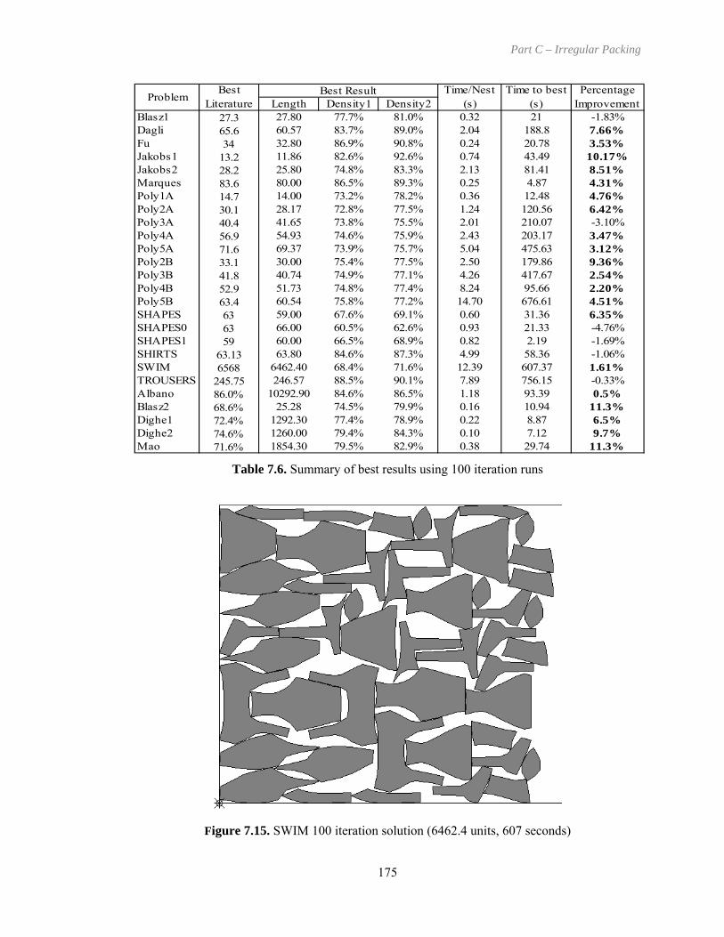
Part C – Irregular Packing
Length Density1 Density2Blasz1 27.3 27.80 77.7% 81.0% 0.32 21 -1.83%Dagli 65.6 60.57 83.7% 89.0% 2.04 188.8 7.66%Fu 34 32.80 86.9% 90.8% 0.24 20.78 3.53%Jakobs1 13.2 11.86 82.6% 92.6% 0.74 43.49 10.17%Jakobs2 28.2 25.80 74.8% 83.3% 2.13 81.41 8.51%Marques 83.6 80.00 86.5% 89.3% 0.25 4.87 4.31%
Poly2A 30.1 28.17 72.8% 77.5% 1.24 120.56 6.42%Poly3A 41.65 73.8% 75.5% 2.01 210.07 -3.10%
Time/Nest Time to best Percentage Problem
Best Best Result
Poly1A 14.7 14.00 73.2% 78.2% 0.36 12.48 4.76%
40.4ly4A 56.9 54.93 74.6% 75.9% 2.43 203.17 3.47%
Poly5A 71.6 69.37 73.9% 75.7% 5.04 475.63 3.12%Poly2B 33.1 30.00 75.4% 77.5% 2.50 179.86 9.36%Poly3B 41.8 40.74 74.9% 77.1% 4.26 417.67 2.54%Poly4B 52.9 51.73 74.8% 77.4% 8.24 95.66 2.20%Poly5B 63.4 60.54 75.8% 77.2% 14.70 676.61 4.51%SHAPES 63 59.00 67.6% 69.1% 0.60 31.36 6.35%SHAPES0 63 66.00 60.5% 62.6% 0.93 21.33 -4.76%SHAPES1 59 60.00 66.5% 68.9% 0.82 2.19 -1.69%SHIRTS 63.13 63.80 84.6% 87.3% 4.99 58.36 -1.06%SWIM 1.61%TROUSERS 245.75 -0.33%
bano 86.0% 10292.90 84.6% 86.5% 1.18 93.39 0.5%Blasz2 68.6% 25.28 74.5% 79.9% 0.16 10.94 11.3%
74.6%
(s) (s) ImprovementLiterature
Po
6568 6462.40 68.4% 71.6% 12.39 607.37246.57 88.5% 90.1% 7.89 756.15
Al
Dighe1 72.4% 1292.30 77.4% 78.9% 0.22 8.87 6.5%Dighe2 1260.00 79.4% 84.3% 0.10 7.12 9.7%Mao 71.6% 1854.30 79.5% 82.9% 0.38 29.74 11.3%
Table 7.6. Summary of best results using 100 iteration runs
Figure 7.15. SWIM 100 iteration solution (6462.4 units, 607 seconds)
175

Part C – Irregular Packing
Further extended experiments were then conducted for the problems in which the approach has
not set new benchmarks namely, Blasz1, SHAPES1, SHIRTS and TROUSERS. For these
runs the durations 551.73s, 2019.77s, 6367.57s and 13613.67s respectively are used as
upper limits in each run, as noted by the authors who have presented the best solutions (previous
to this thesis) for these problems (Gomes & Oliveira, 2002) [172]. For the problems SHAPES
and Poly3A the experiments were extended to 1000 iterations per run, as guidance on
computation times is not available in the literature. The algorithm was allowed a further 10 runs
on each of these benchmark problems for the extended durations specified. Table 7.7 shows the
best results of these runs including the time taken to find the best solution, the method that
generated that solution and percentage improvement on the best known solution. Of the 6
extended experiments, 5 new best benchmark solutions have been set for Blasz1, Poly3A,
SHAPES1, SHIRTS and TROUSERS. For the remaining problem, SHAPES0, the solution
matches the work of [172] (length of 65 units) but has not reached the best known solution of 63
units found in Dowsland & Dowsland (1993) [147]. Note: the approach of chapter nine
consistently improves over the literature best for the SHAPES0 benchmark within three minutes.
extended
Length Density1 Density2Blasz1 27.3 27.47 27.20 79.4% 80.7% Hill Climb/Length 501.91 0.37%Poly3A 40.4 41.45 40.33 76.2% 77.3% Tabu/Area 1515.49 0.18%SHAPES0 63 65.68 65.00 61.4% 63.6% Hill Climb/Area 332.39 -3.17%SHAPES1 59 60.53 58.40 68.3% 71.5% Tabu/Area 1810.14 1.02%SHIRTS 63.13 63.66 63.00 85.7% 88.1% Tabu/Length 806.5 0.21%TROUSERS 245.75 246.40 243.40 89.6% 91.1% Tabu/Area 3611.99 0.96%
Problem Percentage Improvement
Best Literature
Average Length
MethodBest Result Time to best (s)
Table 7.7. Summary of the results from the extended experiments
Of the 26 problems from the literature, using the proposed nesting algorithm, 25 new best
solutions have been produced. The author believes that this is the first time that an irregular
packing approach has attempted such a broad range of problems with such success. The solution
obtained for TROUSERS is shown in figure 7.16. All best solutions obtained for the literature
problems are shown in appendix B.
176

Figure 7.16. TROUSERS extended run solution (243.4 units, 3612 seconds)
nts on New Benchm s
The next set of experiments involved setting initial benchmarks for the new problem
(Profiles1 – Profiles10). Each problem es for 30 minute durations using hill
climbing and tabu search (with both length and area initial orderings) resulting in a total of 40
runs. Table 7.8 shows the results of these experiments, the best solutions are indicated bold
typeface, and table 7.9 is summary of the best results. Figure 7.17 shows the best solutions for
datasets Profiles1 and Profiles9. All best solutions obtained for these new problems also
shown in appendix B.
7.4.2 Experime
Figure 7.17. Best solutions for Profiles1 (1377.74 units) & Profiles9 (1290.67 units)
ark Problem
was run 10 tim
177
Part C – Irregular Packing
instances
in
are

Length Density1 Density2
Leng D1436.3225.8193. 92479.3332. 03146.1309.1341.1314.11555.
BeA a Ord
th ensity1 sit ng y en L nsit ensity2Profiles1 1417.50 1377.74 82.0% 85.2% 1443.21 20 78.4% 80.4% 1 05 % 84. 3.1 1 .1% 82.3%Profiles2 3285.67 3261.00 49.3% 50.5% 3291.01 54 49.8% 51.3 3 16 % 50. 4.8 3 .0% 50.0%Profiles3 8311.23 8228.55 50.7% 51.1% 8252.02 8 50.9% 52.6 8 31 % 51. 2.7 8 .3% 51.7%Profiles4 2489.54 2480.96 74.3% 75.1% 2492.88 30 74.3% 74.8% 2 60 % 75 6.5 24 2 .1% 75.7%Profiles5 3427.47 3360.57 69.6% 73.1% 3381.38 7 70.2% 71.1% 3 52 % 73 3.3 3 .6% 71.3%Profiles6 3180.16 3170.25 73.9% 76.7% 3177.91 82 74.4% 77.5% 3 97 % 77 2.7 3 .5% 77.0%Profiles7 1326.71 1296.30 77.1% 78.3% 1326.57 10 76.4% 80.2 1 09 % 79. 9.9 1 .4% 78.3%Profiles8 1330.88 1318.70 75.8% 77.2% 1361.02 92 74.5% 77.7% 1 22 % 78 5.0 1 .7% 76.4%Profiles9 1341.70 1332.98 51.4% 53.9% 1323.44 97 52.1% 54.3% 1 18 % 54. 5.7 12 7 .1% 54.9%Profiles10 11496.12 11410.60 64.7% 65.5% 11758.50 60 63.9% 64.6% 1 8 6 % 6. 7. 11 0 .9% 64.7%
Problem Resst Result A e Be s ra
gt
Hill Climbing SLength Ordered re ered Le Or a d
Average Length
Best Result Average Length y1 D
ultDen y2 Le th Densit 1 D sity2 ength De
431.45 14 .64 80.3 1% 145 2 427.64 79% 291.86 32 .10 50.0 8% 334 1 280.00 49% 323.90 82 .14 50.7 5% 839 9 290.49 50
488.86 24 .60 74.9 .7% 248 6 53.1 75405.22 33 .90 69.7 .6% 338 1 360.94 69147.11 30 .86 75.6 .8% 316 4 145.76 74
% 324.38 13 .10 76.4 6% 133 9 325.40 75337.57 13 .55 75.6 .0% 135 4 338.47 74350.47 13 .68 51.9 2% 130 0 90.6 531401.2 111 0.10 66.2 6 8% 1165 30 552.3 63
BestveragLength
st Re ult Ave ge Len h
Tabu earchngth dered Are Ordere
Table ents on ne n ark problems
7.8. Experim w be chm
Length Density De sity22.0% 8 2%0.0% 5 3%0.9% 5 6%5.1% 7 7%0.2% 7 6%5.6% 7 8%7.1% 8 2%5.8% 7 2%3.1% 5 9%6.2% 6 8%
Res1 n
le 1377.74 8 5.le 3216.10 5 1.le 8193.89 5 2.
Profile 2453.12 7 5.Profile 3332.70 7 3.Profile 3097.86 7 7.Profile 1296.30 7 0.Profile 1318.70 7 7.Profile 1290.67 5 4.Profile 11160.10 6 6.
le Best ult
Profi s1Profi s2Profi s3
s4s5s6s7s8s9s10
Prob m
Table 7.9. Summa best results e n ark problemsfor n w be chmry of
Part C – Irregular Packing
7.5 Summary
In this chapter, a new technique of primitive overlap resolution was introduced and it was
nerated that is able
to handle profiles with both circular arcs and holes. This algorithm produces layouts for realistic
ccuracy that makes it a strong candidate for industrial
een applied to 26 problems drawn from over 20 years
of cutting and packing research and, using only simple local search mechanisms, was able to
produce the best-known results for 25 of the 26 problems. The majority of these best solutions
were generated within 100 search iterations and yielded an average improvement of 5% over the
existing best solutions from the literature. Finally, the chapter introduced 10 new problems,
some of which involve profiles with both arcs and holes that have not previously been
represented within the literature, and set initial benchmark solutions to facilitate further
comparisons.
To the author’s knowledge this is the first time that an automated approach has attempted such a
broad range of problems from the literature and with such success.
demonstrated how an efficient bottom-left-fill nesting algorithm could be ge
problems both quickly and to a level of a
application. The proposed algorithm has b
179

Part C – Irregular Packing
CHAPTER EIGHT
degenerate shape cases and shapes involving holes.
, reasonable generation times are reported for the set of benchmark data that include
datasets of tables 2.3 & 2.4 and new benchmark
problems, Profiles6 – Profiles10).
ped during this work. It is also beneficial to
implement routines th ord promote fast no-fit
The No-Fit Polygon: A Robust
Implementation
Chapter six focussed on the geometric difficulties that this research has faced with specific
attention given to the no-fit polygon. The previous generation approaches were also discussed
with the main point that they all have disadvantages or degenerate shapes that cannot be
handled. In this chapter, a new no-fit polygon generation approach is presented that modifies
and extends the orbital trigonometry approach (as used by Mahadevan in 1984 [256]).
Furthermore, examples are provided to show how the developed approach is able to robustly
generate no-fit polygons for several known
Finally
shapes consisting of lines (all of the literature
8.1 The New No-Fit Polygon Construction Algorithm
For the intersection calculations within this presented implementation, it is important to use a
robust geometry library such as the one develo
at are as fast and optimised as possible in er to
polygon generation and packing algorithms. Once again, the author recommends that
practitioners who do not wish to develop such a library use the geometry modules of the LEDA
and CGAL libraries.
180

Part C – Irregular Packing
8.1.1 Overview
The new approach can be divided into two logical stages. Section 8.2 describes the procedure
gon slides around another to create the outer path of no-fit
ygon (i.e.
ontained by the outer path) and are not found using Mahadevan’s algorithm alone. For this
section we will ass polygons, A and B, that exist
somewhere within the no-fit polygon
NFPAB (orbiting po n that must be performed is to
translate polygon olygon A. This can be
achieved by transl is placed at the lowest y-
coordinate of polygon A (see figure 8.1).
Figure 8.1. Initial translation of the orbiting polygon to touch the stationary polygon
for the first of these where one poly
polygon of the two shapes. This follows a similar approach to that of Mahadevan’s algorithm
although a modified implementation is proposed. The second section introduces the notion and
identification of starting positions that allow the algorithm to find the remaining paths of the no-
fit polygon (see section 8.3). These paths will be internal holes of the no-fit pol
c
ume that we have two anticlockwise oriented
two-dimensional space and we are required to produce
lygon B around polygon A). The first operatio
B such that it is touching, but not intersecting, p
ating polygon B such that its largest y-coordinate
A B
PtB(ymax)
B A Trans
PtA(ymin)
A
B
181

Part C – Irregular Packing
Using these two verti and B will be non-
intersecting and touching. The translation at results in polygon B touching (but not
The main aim of the orbiting (or sliding) section of the algorithm is to detect the correct
movements that B must move to traverse around A in order to return to its original position.
This is an iterative procedure with each translation step creating an edge of the no-fit polygon.
This can be broken down into the following subparts which will be discussed in turn:
Section 8.2.1 - Detection of Touching Edges
Section 8.2.2 - Creation of Potential Translation Vectors
Section 8.2.3 - Finding a Feasible Translation
Section 8.2.4 - Trimming the Feasible Translation
Section 8.2.5 - Applying the Feasible Translation
8.2.1 Detection of Touching Edges
The ability to correctly detect touching and intersecting edges is paramount to the success of this
approach. This is achieved by testing each edge of polygon A against each edge of polygon B.
ces for alignment guarantees that polygons A
th
intersecting) polygon A is given by formula (1):
Trans B A = PtA(ymin) – PtB(ymax) (1)
In reality, any starting position may be used providing that it results in polygons A and B
touching and not intersecting. The orbital approach can now commence to generate the outer
path of the no-fit polygon by orbiting polygon B in an anticlockwise direction.
8.2 Orbiting / Sliding
182

Part C – Irregular Packing
Each pair of edges that touch (one from polygon A and one from polygon B) is stored along
with the position of the touching vertex.
Figure 8.2. Identification of touching edge pairs
Figure 8.2 shows the resulting set of touching edge pairs. This is in contrast to the approach of
Mahadevan who performs calculations using all edges at a touching vertex. For example on
figure 8.2, Mahadevan would present edges a2, a3, b1 and b4 on the same diagram. In the
authors experience with such algorithms, this makes the required calculations more complicated
and difficult to explain. These edge-pair diagrams will be used in the next stages to create the
potential translation vectors for polygon B and to eliminate the non-viable translation vectors.
8.2.2 Creation of Potential Translation Vectors
The vector with which polygon B must be translated to orbit polygon A must either be derived
from an edge of polygon A or from polygon B depending on the situation. Figure 8.3 shows an
example of each case. Note that in the second case (figure 8.3b), because polygon B slides
along one of its own edges, the translation vector is found by reversing the edge. This is further
examine on A is
latively moved along the edge b1. In reality, polygon A must remain fixed and B must be
translated and therefore, the translation vector is reversed in this situation.
A
B b1
b2b3
a
a2
a
a5
a6a7
b4
1
a3
4
a2
b1
a2
b4
a3b1
a3
b4
d through the relative movement of the polygon A with respect to B. Polyg
re
183
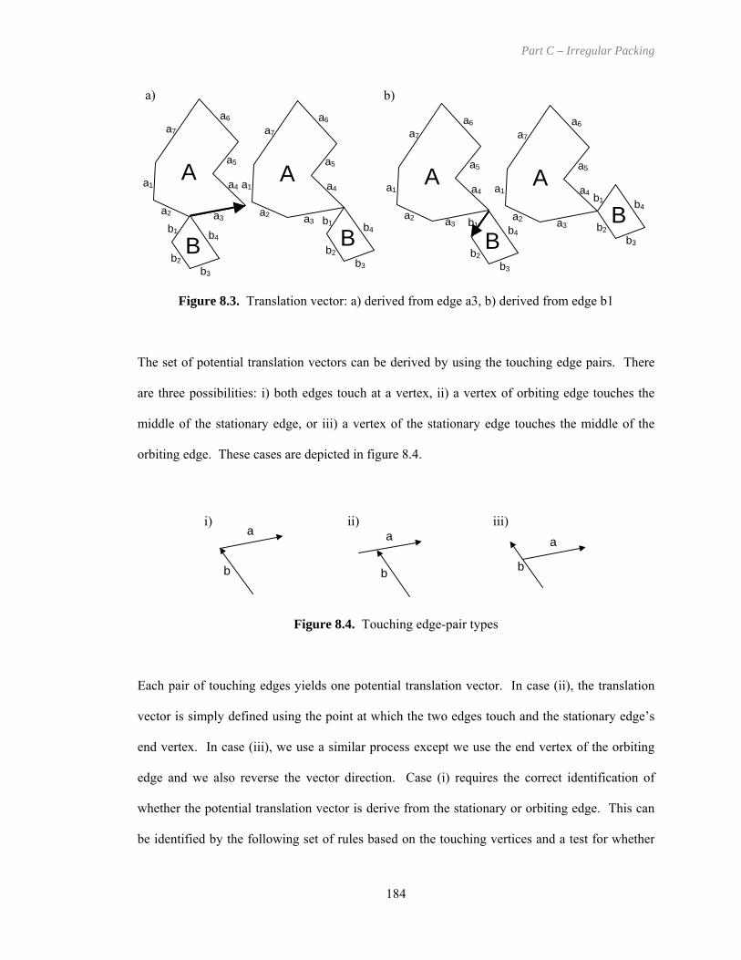
Part C – Irregular Packing
A
Figure 8.3. Translation vector: a) derived from edge a3, b) derived from edge b1
A
B b
bb
1
2
b
3
4
a1
a2 a3
a4
a5
a6a7
Bb1
b2b3
4b
a1
a2 a3
a4
a5
a6a7
A
Bb1
b2b
b4
3
a1
a2
a4
a5
a6a7
A B
b
bb
1
2
b
7
3
4
a1
a2 a3
a4
a5
a6a
b)a)
a3
The set of potential translation vectors can be derived by using the touching edge pairs. There
are three possibilities: i) both edges touch at a vertex, ii) a vertex of orbiting edge touches the
middle of the stationary edge, or iii) a vertex of the stationary edge touches the middle of the
orbiting edge. These cases are depicted in figure 8.4.
dentification of
hether the potential translation vector is derive from the stationary or orbiting edge. This can
n the touching vertices and a test for whether
Figure 8.4. Touching edge-pair types
Each pair of touching edges yields one potential translation vector. In case (ii), the translation
vector is simply defined using the point at which the two edges touch and the stationary edge’s
end vertex. In case (iii), we use a similar process except we use the end vertex of the orbiting
edge and we also reverse the vector direction. Case (i) requires the correct i
w
be identified by the following set of rules based o
a
b
aiii)i) ii)
a
b b
184

Part C – Irregular Packing
the orbiting edge, b, is left or right of the stationary edge, a. Table 8.1 shows the different
possibilities and the edge from which a potential translation vector is derived under each
circumstance.
Stationary Orbiting
1 Start Start Left Orbiting Edge
2 Start Start Right Stationary Edge
3 Start End
Touching Edge Vertex Relative Position of the Orbiting Edge to the Stationar
y Edge
Translatio Derived FromCase
Left -
5 End Start Left -
8 Parallel Either Edge
4 Start End Right Stationary Edge
6 End Start Right Orbiting Edge
7 End End -
n
Table 8.1. Deriving the potential translation when both edges touch at vertices
Clarification is now given as to why some potential translations can be eliminated in certain
cases of the table (an ‘-‘ entry in the table indicates that no translation is derived). Remember
that a translation that is derived from an edge is the resultant vector defined by touching point
end vertex (and then the vector is reversed for an orbiting edge). This allows the elimination of
case 7 of the table because both the stationary and orbiting edges touch on the end vertices and
this would yield a null translation vector. In cases 3 and 4, the orbiting edge touches at its end
vertex thus a translation cannot be derived from the orbiting edge. In cases 5 and 6, the
stationary edge cannot be used as it would produce a null vector. Figure 8.5 shows an example
for each of the cases using two polygons that touch at two separate places.
185

Part C – Irregular Packing
186
Case Edges Derived From1 (a3,b3) b3
2 (a1,b4) a1
3 (a3
4 (a1
,b2) -,b3) a1
5 (a5,b4) -6 (a2,b3) b3
7 (a2,b2) , (a5,b3) -
Figure 8.5. Two polygons touching at two separate positions and vertex-vertex touch cases
In cases 3 and 5, no translation can be derived because the edge of the orbiting polygon is left of
the edge from the stationary polygon. For example, edges a3 and b2 touch on their start and end
vertices respectively. As a null translation is produced using edge b2 (due to touching with the
end vertex), the only possibility is to derive a translation vector from the stationary edge, a3.
However, edge b2 is left of edge a3 and, if this translation vector were used, edge b2 would slide
along the inside of edge a3. Therefore, the positional “left test” eliminates the translations
whereby polygons tside of the edge.
Where edges are parallel, either the stationary or the orbiting edge may be used.
ersection. For example, returning to
igure 8.5, two potential translation vectors, a1 and -b3, have been generated. It can easily be
een that the orbiting polygon B must be translated using vector -b3 in order to move
nticlockwise around polygon A. If polygon B was to be translated along vector a1 instead, this
would result in an immediate intersection between edges a2 and b3 (and also a3 and b3). Once
again the set of touching edge-pairs, generated from section 8.2.1, contains all of the information
needed to determine a feasible translation vector.
A Ba1
a4
a5
b1
2
b4
2
a3
a
b3
b
would slide along the inside of an edge rather than the ou
8.2.3 Finding a Feasible Translation Vector
Once the potential translation vectors have been produced, the next stage is to select a
translation vector that does not result in an immediate int
f
s
a

Part C – Irregular Packing
The process here is simplified due to the proposed representation of touching edges and involves
h are not shown. These have been omitted for
brevity and because they are reasonably straightforward (the examples shown in figure 8.6
provide enough
3 and a1, were calculated for two touching polygons. Figure 8.7 uses the
1
1
1
taking each of the potential translation vectors in turn (identified in section 8.2.2) and placing
them on the touching position at each touching edge-pair. Positional relationships between the
stationary and orbiting edge can be defined based on the union of left/right regions that indicate
whether a particular potential translation will be suitable for those edges. For a potential
translation vector to be identified as feasible, it must be suitable for every pair of touching
edges. Figure 8.6 shows some examples of touching edge-pairs and the angular range of
feasible translations.
a a a a a a
Figure 8.6. Identifying the feasible angular range of translations (indicated by the arc)
b b b b b b
aright
∪ bright
aright
∪ bleft
aleft
∪ bright
aleft
∪ bleft
aright
bleft
There are other possibilities that can occur whic
information to derive the omitted relationships). In figure 8.5 two potential
translation vectors, –b
same example to demonstrate how the approach eliminates translation vector a (the edge-pairs
involving edge a have been omitted for brevity but these will be feasible translations because
the translation vector is also a ). In reality, once a potential translation fails on one of these
inated without further testing. tests, it is infeasible and can be elim
187

Part C – Irregular Packing
188
a3
a2
a4a5
a6
a
a10
a14
16
a1
b
Figure 8.7. Elimination of potential translation vector, a1
t this stage, one (or more) feasible translation vectors have been found. Usually there will only
an actual screenshot taken from the implementation). The reference point of
present, the edge that is nearest (in edge order) to the previous move is chosen. Therefore,
a7a9
8
a12a11
a13
a15
a
b1
b2
3
b4
A
be one translation vector but several may be present under the special circumstances as shown in
figure 8.8 (this was
the orbiting square has been set to the centre to aid clarity.
Figure 8.8. Two polygons involving exactly fitting ‘passageways’
This introduces another important aspect of the algorithm; we must maintain the edge that was
used to generate the previous translation vector. When several feasible translation vectors are
a2
b3
a3
A B a1
a4
a5
2
bb3
2
a3
a
b3
b1
b
4
Transa1 a1TransInfeasible Edge Translations
a2b2 a5
b3
a5 b4
Transa1 Transa1Transa1 a3
b2
Transa1
FeT
asible Edge ranslations

Part C – Irregular Packing
returning to figure 8.8, the square enters the passageway using edge a3 instead of sliding straight
8.2.4 Trimming the Feasible Translation Vector
B can be translated is to trim the translation vector. This important
Figure 8.9. A translation vector that requires ‘trimming’ to avoid intersection
In order to find the correct non-intersecting translation the translation vector is projected at each
of the vertices of po on B and is tested for intersection with all edges of polygon A. This
ensures that we correctly identify the vertices of polygon B that will cross into polygon A and
reduce the translation distance accordingly using formula (2).
over the opening using edge a14. Then, after sliding into the centre of the stationary polygon, the
square has four feasible translation vectors derived from edges a4, a7, a10 and a13. However, the
translation vector derived from edge a4 will be used because the edge that was used previously
was a3. This is another modification that has been made to the approach of Mahadevan.
The last step before polygon
because there may be other edges that can interfere with the translation of the orbiting polygon.
Figure 8.9a provides an example whereby applying the entire translation vector results in the
two shapes intersecting. In order to prevent the orbiting polygon entering the body of the
stationary polygon, the feasible translation, a7, must be trimmed to edge a1 (see figure 8.9b).
A B
A Ba
a
1
2a
a
3
a 6
a
a5
a74
5a
7
a1
a2a3
a4
a6
A A B
a
B
a5
a7
a5
a7
1
a2a3
a4
a6
a1
a2a3
a4
a6
b)a)
lyg
New Translation = IntersectionPt – TranslationStartPt (2)
189

Part C – Irregular Packing
The translation vector must also be projected back from all vertices of polygon A (by translating
the end vertex of the translation vector onto each vertex) and then test for intersection with all
edges of polygon B to examine if any will cross into polygon B. This is depicted in figure 8.10
using the same example but a different orbiting polygon.
a)
Figure 8.10. Trimming with projections from polygon A
completed. As the proposed algorithm trims at every intersection, the translation vector
considerably faster than performing full line intersection routines. The approach of Mahadevan
Once again, if there is an intersection, the translation distance should be reduced to reflect this
using formula (3).
New Translation = TranslationEndPt – IntersectionPt (3)
The new approach is fundamentally the same as used by Mahadevan except that the translation
vector is trimmed at the time of intersection whereas Mahadevan keeps the translation vector the
same but stores the minimal intersection distance and trims once after all projections have been
becomes shorter throughout the testing process which can reduce the number of intersections
that occur due to fast elimination tests through the use of bounding boxes which are
may need to calculate several more full intersection tests because the entire translation vector is
used at each projection and thus could potentially require more computation.
A Ab2b3
b)
B A A
b1
b2b3
Bb1
b2b3
B b1
b2b3 Bb1
190

Part C – Irregular Packing
8.2.5 Applying the Feasible Translation Vector
The final step is to append the trimmed translation vector to the end of the partial no-fit polygon
reated so far and polygon B is translated by the trimmed translation vector. This will move the
gon to the next ‘decision’ point and the process can restart from the detection of touching
edges (section 8.2.1). The only nuance to this proces that a test mu e p formed to detect
if the reference point of polygon B has returned to its initial starting position.
8.3 Start ts
Section 8.2 identified an approach for the orbiting of one polygon around another using edge
c
proposed by Mahadevan [256]. Howe ents have been proposed that result in
e procedure requiring less computation and allow the approach to be explained more easily.
c
poly
s is st b er
Poin
omparisons and edge sliding. The overall effect of the approach is similar to the algorithm
ver, some improvem
th
Therefore, the proposed approach currently has the same limitations as Mahadevan’s approach
(the inability to generate complete no-fit polygons for shapes involving interlocking concavities,
jigsaw pieces or holes). Figure 8.11a shows two polygons for which the sliding algorithm alone
does not produce the complete no-fit polygon. The polygons have concavities that can interlock
with each other to create a further no-fit polygon region but this is never found because of the
narrow entrance to the stationary polygon’s concavity (see figure 8.11b).
Figure 8.11. Interlocking concavities: a) polygons, b) no-fit polygon using sliding alone, c) the
complete no-fit polygon
b)a) c)
a
a1
2
a3
56
a8
a1
a3
56
a8
1
3
a a8
a4
aa
a7
a9
a2
a4
aa
a7
a9
a
a2
aa4
a5a6
7
a9A
B
A A
B B
191

Part C – Irregular Packing
In this section, an approach is given based on the identification of feasible touching but non-
intersecting start positions with which the previously described sliding technique can be
e yed to generate the remaining inner loops no-fit polygon construct. For example, if
polygon B can be placed in the location shown in figure 8.11c, then the sliding algorithm can be
employed (without change) t the internal no-fit polygon region (note that this loop
will be a clockwise loop indicating that it is an inner-fit polygon region). Feasible starting
odification of the approach detailed in section 8.2. Once again,
involves iding one polygon around the edges of the other. However, we are not interested
in sliding to trace the no-fit polygon but to resolve edge intersections whilst translating along a
particular edge vector.
I r to explain the process, an example of finding the start positions along one edge of
polygon A is given. This h edge of polygon A and
, e,
n B intersects with polygon A then further testing and edge sliding must
e performed to traverse along edge e until a non-intersecting position is found or the end of the
mplo of the
o generate
positions are found through a m
this sl
n orde
process can then easily be reproduced for eac
polygon B to create all feasible starting positions to allow polygon B to o it around polygon A
in order to create the entire no-fit polygon.
G n an edge of p gon A, the potential starting positions of an orbiting polygon B along e
can be found. The process involves translating polygon B such that each of its vertices, in turn,
are aligned to the start vertex of e. The following steps are performed for each position. If the
polygons do not intersect in this position, then this is noted as a feasible start position for the
two polygons. If polygo
rb
ive oly
b
edge is reached. In such an instance, the first test involves examining whether the two
connected edges of polygon B (joined at the touching vertex) are both right or parallel to the
edge e. If either of polygon B’s connected edges are left of e then they will translate on the
192

Part C – Irregular Packing
inside of polygon A and can be eliminated immediately because sliding along the vector derived
from edge e will never yield a feasible starting position.
Figure 8.12a shows an example of where the connected edge pair, b3 and b4, are eliminated from
sliding along a5 because b4 is left of a5 (note that this will not be eliminated when using edge b4
of the polygon B and connected edges a4 and a5 of polygon A). Figure 8.12b shows an example
of where both connected edges, b1 and b2, are right of edge a5.
Figure 8.12. Vertex alignment of polygon B to polygon A using edge a5: a) invalid alignment,
b) valid alignment
Now assuming both connected edges are right of edge e and polygons A and B intersect we can
attempt to resolve the overlap by translating the orbiting polygon along the translation vector
defined by e. As with the previous section, trimming can now be employed to this vector (the
procedure is identical). The resultant translation vector can then be applied to slide polygon B
along edge e and then another intersection test is performed. If the two polygons still intersect
then the process repeats with the translation vector derived from the touching point to the end
vertex of edge e. If the intersection has been resolved then the reference point of polygon B is a
potential start position. If the entirety of edge e is traversed and there is still an intersection then
no feasible starting position can be found along edge e and the aligned vertex / connected edges
a2
a3
a4
a5
a6
a7
a8
a9A
a1
B b1
b2
b3
b4
b5
b6 a2
a3
a5a6
a7
a8
A
a1
a4
a9
B
b2
b3b4
b5
b6
b1
b4
b3
a5
b2b1
a5
b)a)
193

Part C – Irregular Packing
of polygon B. The next vertex of polygon B is then considered and so forth until all edge vertex
ined. Note it is also important to examine the edges of polygon B
presented in figure 8.12b. When aligned using a5
edges b1 and b2, the two polygons are initially intersecting so we need
d from edge a5.
possibilities have been exam
with the vertices from polygon A but as this is an identical procedure and will not be discussed.
Figure 8.13 shows this process on the example
and the vertex connecting
to resolve the intersection along the vector derive
ab)a)
Figure 8.13. Start point generation process
a2
a3
a4
a5a6
a7
a9A
1
b1 b2
b b
b6
3 b45
a2
a3
a4
a
a7
a9
a56
A
a1
b1 bb
2 b4
b5
b6B
a8
3
Ba8
Pt
a2
a4
aa56
a7
a9A
a1d)c)
b1 b2 b4b3 b5
b6B
a
a4
a5a6
a9
a
2
a7
1
b1 b2 b3 b4b5
b6
Aa8 a8Pt
B
a3 a3
194

Part C – Irregular Packing
Figure 8.13a shows the trimming process and identification of the closest intersection point, Pt.
lygon B is then translated by the trimmed translation vector. The resulting position is shown
e touching point to the end vertex of edge a5 and is then
the important trim is shown). After applying this
tion to polygon B, the polygons are no longer intersecting and therefore a feasible start
dard orbital approach can be employed once more to generate
n the implementation is that the outer no-fit polygon
loop is calculated using the approach in section 8.2 and then the starting position procedure is
applied n A and polygon B in turn.
During the process, as soon as a feasible start position is found, the inner loop of the no-fit
lygon e flagged as they
t points which
already t have already been calculated.
a more edges become flagged as new no-
fit poly ps are produced, thus reducing the computational requirements for generating
new fea or no more
le and the complete no-fit polygon is returned.
Po
in figure 8.13b. The polygons are still intersecting so the procedure must be repeated. The
translation vector is calculated from th
trimmed as shown in figure 8.13c (only
transla
point has been found and the stan
the no-fit polygon loop.
An optimisation that has been included i
on the untraversed / unflagged edges from both polygo
po can be calculated using the orbital algorithm (as before, the edges ar
are traversed). This ensures that the algorithm does not attempt to find star
exist w thin one of the no-fit polygon loops thai
Therefore, this voids unnecessary calculations because
gon loo
sible start positions. The procedure repeats until all edges have been seen
feasible rt positions are availabsta
195

Part C – Irregular Packing
8.4 Pseudocode
The no-fit polygon algorithm can be described using the following pseudocode given the
functionality outlined in the previous sections:
PtB(ymax) = point of maximum x value of polygon B
Point NFPLoopStartRefPoint;
er of loops in NFP
A(ymin) B(ymax)
// Sort trimmed translations by length Touchers[] lengthSortedTouchers = Sort(trimmedTouchers);
//Translate polygon B along longest feasible translation vector B.Translate(lengthSortedTouchers[0].T
// Add translation to nfpEdges[loopCount].A A.MarkEdge(lengthSortedTranslations[0].StaticEdgeID);
if(NFPLoopStartRefPoint == PolygonB_RefPoint / co eted an NFP loop
; // find next feasible start point – reset PolygonB_RefPoint to relevant point
if(bStartPointExist)
B.Translate(PolygonB_RefPoint - nextStartPoint);
loopCount++;
else
}
NFPAB = Complete(nfpEdges); //Reconstitute NFP from nfpEdges
nd
Input : Polygons A and B PtA(ymin) = point of minimum x value of polygon A
IFP = initial feasible position Bool bStartPointAvailable = true;
Point PolygonB_RefPoint; Array[Line[]] nfpEdges; // an array of arrays of lines to store NFP edges Int loopCount = 0; // counter for numb Begin Place polygons in IFP using translation Pt – PtNFPLoopStartRefPoint = PtB(ymax); PolygonB_RefPoint = PtB(ymax); While(bStartPointAvailable) { bStartPointAvailable = false; // find touching segments & touching points on those, generate touching structures Touchers[] toucherStructures = FindTouchers(A, B);
// Eliminate non feasible touchers, ones that cause immediate intersection Touchers[] feasibleTouchers = CanMove(A, B, toucherStructures);
// Trim feasible translations against polygon A and B Touchers[] trimmedTouchers = Trim(feasibleTouchers, A, B);
ranslation);
nfpEdges & mark traversed edge on static dd(lengthSortedTranslations[0].Translation);
) / mpl { Point nextStartPoint
bStartPointExists = FindNextStartPoint(A,B,&nextStartPoint, &PolygonB_RefPoint);
{ //Translate polygon B to nextStartPoint
NFPLoopStartRefPoint = nextStartPoint;
} }
{ bStartPointAvailable = true; // allow edge traversal to continue
}
E
196
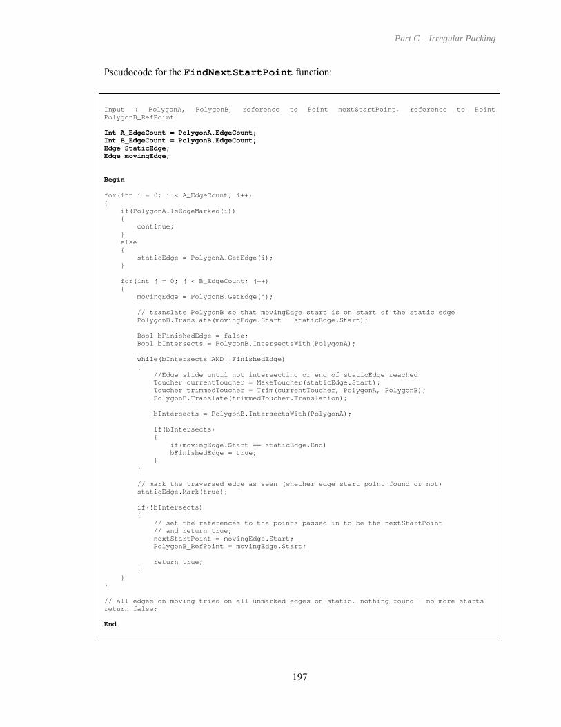
Part C – Irregular Packing
197
Pseudocode for the FindNextStartPoint function:
staticEdge = PolygonA.GetEdge(i); }
r( ; j++)
movingEdge = PolygonB.GetEdge(j);
PolygonB.Translate(movingEdge.Start – staticEdge.Start);
{
turn false;
Input : PolygonA, PolygonB, reference to Point nextStartPoint, reference to Point PolygonB_RefPoint Int A_EdgeCount = PolygonA.EdgeCount; Int B_EdgeCount = PolygonB.EdgeCount; Edge StaticEdge; Edge movingEdge; Begin for(int i = 0; i < A_EdgeCount; i++) { if(PolygonA.IsEdgeMarked(i)) { continue; } else {
fo int j = 0; j < B_EdgeCount {
// translate PolygonB so that movingEdge start is on start of the static edge
Bool bFinishedEdge = false; Bool bIntersects = PolygonB.IntersectsWith(PolygonA);
while(bIntersects AND !FinishedEdge)
//Edge slide until not intersecting or end of staticEdge reached Toucher currentToucher = MakeToucher(staticEdge.Start); Toucher trimmedToucher = Trim(currentToucher, PolygonA, PolygonB); PolygonB.Translate(trimmedToucher.Translation);
bIntersects = PolygonB.IntersectsWith(PolygonA);
if(bIntersects) {
if(movingEdge.Start == staticEdge.End) bFinishedEdge = true;
} } // mark the traversed edge as seen (whether edge start point found or not) staticEdge.Mark(true);
if(!bIntersects)
{ // set the references to the points passed in to be the nextStartPoint // and return true; nextStartPoint = movingEdge.Start; PolygonB_RefPoint = movingEdge.Start;
return true;
} } } // all edges on moving tried on all unmarked edges on static, nothing found – no more starts re End

Part C – Irregular Packing
8.5 Problem Cases
In this section each of the problem cases that cause difficulties with other methods are discussed
and it is shown how the proposed algorithm is able to handle them without specific case-by-case
implementations. In each figure of this section, the stationary and orbiting polygons are
represented by dark and light grey shading respectively and the reference point of the orbiting
polygon is shown as a black dot. This is used to trace the no-fit polygon loops (numbered).
8.5.1 Interlocking Concavities
pical problem case for the previous orbital sliding
concavities and, therefore, multiple feasible start points. The no-fit polygon of these two shapes
The interlocking of concavities is a ty
approaches of the literature such as (Mahadevan, 1984). Figure 8.14 displays a screenshot after
the algorithm has generated the complete no-fit polygon of identical shapes with one rotated
through 180°. The shapes in these orientations involve many different interactions of the
results in six loops within the no-fit polygon (one outer loop, 1, and five internal loops, 2-6).
Figure 8.14. Multiple interlocking position
1
4
6
2
35
198
s

Part C – Irregular Packing
8.5.2 Exact Fit: Sliding
The next case involves the sliding through exactly fitting “passageways” which cannot be
handled by either the Minkowski sum approach of (Bennell, Dowsland and Dowsland, 2001) or
the orbital approach given in (Mahadevan, 1984). An extension was proposed to Mahadevan’s
algorithm (in section 8.2.3) that can deal with such problems through the maintenance of the
previously traversed edge which enables consecutive edges of the stationary polygon to be used
in the next translation iteration. An example is shown in figure 8.15 (also see figure 8.8).
1
Figure 8.15. Exact fit sliding through a “passageway”
8.5.3 Exact Fit: Jigsaw Pieces
The problem case involving jigsaw pieces that link together exactly (also called “lock-and-key”)
is another form of the interlocking concavity case. However, the distinguishing feature of
jigsaw pieces is that they fit together with no movement, thus creating a singular feasible point
within the no-fit polygon (rather than an internal loop in the interlocking concavity case). In the
proposed approach, this position is found by the generation of feasible starting positions. Of
course, the algorithm will still try to slide the orbiting polygon along edges but, in this case,
there is no feasible translation vector which distinguishes that this position is just a singular
feasible point location (see figure 8.16). Most of the previous approaches have suffered from
199

Part C – Irregular Packing
such degeneracy including: the Minkowski sum approach where no boundary exists to identify
lock-and-key positions within the no-fit polygon, digitisation which suffers from loss of
accuracy, convex decomposition whereby it is not possible to find such positions through
recombination alone and the sliding algorithm of Mahadevan (which suffers identical difficulties
to that of interlocking concavities).
Singular Feasible
Point
1
a) b)
2
Figure 8.16. Jigsaw pieces: a
8.5.4 Holes
There hav
by the conca
aps within the larger hole of the sta
e been few approaches
containing holes. This could be du
involving holes. However, throug
polygon can be generated easily a
example involving a shape with two
regions of the holes. The figure s
concavities: loop 1 is the outer no-fi
4 and 8 are cases where
g
1
2
) outer NFP loop, b) singular feasible internal position
al sha
vity of the smaller orbiting shape interacts with the narr
tionary shape.
within the literature that operate on polygon
e to the difficulty of generation process for no-fit polygo
h the detection of feasible starting positions, the no
nd, more importantly, completely. Figure 8.17 shows
holes and a shape that can be placed within several disti
hows a mixture of cases involving holes and interlock
t polygon loop, loops 2,3,5,6,7 are all hole cases, and loo
200
pes
ow
ns
-fit
an
nct
ing
ps

Part C – Irregular Packing
201
1
4
5
6
23
7
8
Figure 8.17. No-fit polygon of two polygons, one of which involve
Convex decompositions can result in a larger number of pieces and becom
the introduction of holes. Therefore union or recombination is also com
larger number of intersecting sub-no-fit polygon elements that ne
Digitisation can generate no-fit polygons with holes but this is achieved w
the discretisation of a continuous space. The phi-function approach of S
m
will ultimatel
erformed (especially with very complex shapes). Previous orbital a
any of the degeneracies through the resolution of primary objects. H
y impact on the efficiency of intersection testing as many
p
produced the outer no-fit polygon loop and Minkowski sum approaches
due to the untangling of edges. The author is unaware of any previous no-
methods that have specifically presented no-fit polygon constructs for s
degeneracies.
s multiple holes
e more difficult with
promised due to the
ed to be untangled.
ith inaccuracy due to
toyan could deal with
pproaches have only
owever, this approach
separate tests must be
can become difficult
fit polygon generation
hapes involving such

Part C – Irregular Packing
8.6 Generation Times on the Benchmark Data
In order to demonstrate the speed and capabilities of the proposed no-fit polygon procedure, the
es for all of the literature benchmarks of table 2.3 & 2.4 and the new benchmark
problems containing shapes consisting of lines only, Profiles5 – Profiles10 are reported. For
each problem the total generation time and number of no-fit polygons generated per second are
given (see table 8.2). The “Logical Total Number of Shapes” (column E) is found by E = B * D
F = E2 . All experiments have
been conducted on a Pentium 4 2GHz processor with 256MB RAM.
generation tim
and the “Total Number of NFPs” (column F) is calculated by
A B C D E F G H
DatasetNumber of Different Shapes
Rotational Number of Rotations per Shape
Logical Total Number of
Shapes
Total Number Total
Generation Time (s)
NFPs Per
Albano180 8 180 2 16 256 0.32 800
Blasz1 7 180 2 14 196 0.21 933
Dagli 10 90 4 40 1600 0.93 1720Dighe1 16 90 4 64 4096 1.28 3200Dighe2 10 90 4 40 1600 0.62 2581
Fu 12 90 4 48 2304 0.52 4431
Jakobs2 25 90 4 100 10000Mao 9 90 4 36 1296
Constraints of NFPs Second
Albano90 8 90 4 32 1024 0.71 1442
Blasz2 4 90 4 16 256 0.19 1347
Jakobs1 25 90 4 100 10000 5.57 17955.07 19721.41 919
Marques 8 90 4 32 1024 0.79 1296Poly1a 15 90 4 60 3600 1.37 2628
Poly4a 15 90 4 60 3600 1.37 2628
Poly5b 75 90 4 300 90000 141.90 634
Shapes0 4 0 1 4 16 0.11 145
Profiles6 9 90 4 36 1296 0.86 1507s7 9 90 4 36 1296 0.58 2234
Profiles8 9 90 4 36 1296 0.56 2314Profiles9 16 90 4 64 4096 44.30 92Profiles10 13 0 1 13 169 0.55 307
Poly2a 15 90 4 60 3600 1.37 2628Poly3a 15 90 4 60 3600 1.37 2628
Poly5a 15 90 4 60 3600 1.37 2628Poly2b 30 90 4 120 14400 7.54 1910Poly3b 45 90 4 180 32400 27.14 1194Poly4b 60 90 4 240 57600 68.45 841
Shapes 4 90 4 16 256 0.38 674
Shapes1 4 180 2 8 64 0.19 337Shirts 8 180 2 16 256 0.33 776Swim 10 180 2 20 400 6.08 66
Trousers 17 180 2 34 1156 0.73 1584
Profile
Table 8.2. No-fit polygon generation times for 32 datasets of the literature
202

Part C – Irregular Packing
Table 8.2 shows that the no-fit polygon constructs can be generated within reasonable time
frames on most of the benchmark data. Typically the algorithm can generate about 1000 no-fit
polygons per second although this can vary drastically depending on the number of line
segments in each problem. For example, the two problems with the lowest no-fit polygons
generated per second, “Swim” and “Profiles9”, involve pieces with many line segments (up to
7) due to approximation of arcs and, further to this, “Profiles9” contains several shapes with
holes (see figure 8.18).
6
Figure 8.18. A selection of pieces and no-fit polygons from the “Profiles 9” (letters) and
“Swim” datasets
The slowest overall generation times occur within the Poly4b and Poly5b problems and are
simply due to the large number of no-fit polygons that must be generated. As mentioned in
section 8.3.2, other reported generation times for available benchmark problems of the literature
can be found in Bennell, Dowsland and Dowsland (2001) [239]. Table 8.3 shows a comparison
of the generation times of the new orbital approach to the Minkowski based approach of
Bennell, Dowsland and Dowsland using a DEC Alpha 3000/400. Each problem is set to use 0°
203

Part C – Irregular Packing
rotations for comparative purposes (polygons in the orientation they are drawn) as this was the
rotational constraint that was used in Bennell, Dowsland and Dowsland (2001).
Minkowski Approach (Bennell et al, 2002)
Orbital Approach (Presented)
DS1 0.32 0.23DS2 0.22 0.04
DS3
Dataset Total Generation Times (seconds)
(Shirts) 0.23 0.17DS4 (Shapes0) 0.38 0.11DS5 (Blasz1) 0.36 0.13
(0° rotation only)
Table 8.3. Comparison of generation times of the Minkowski approach of Bennell, Dowsland
and Dowsland (2001) with the presented orbital approach on 5 literature datasets.
The table shows that the new orbital approach generates the no-fit polygons quicker than the
Minkowski sum approach for all of the five datasets. Although there is an obvious difference in
the computing power available to the two approaches, the fact that they both perform with very
quick execution times shows that the overhead incurred in generating no-fit polygons is almost
negligible. The proposed algorithm is able to quickly and robustly generate all of the no-fit
polygons for the literature benchmark problems (including several datasets from the textiles and
metal cutting industries).
Whilst very large problems may require a few minutes to generate all of no-fit polygons, such as
the Poly4b and Poly5b test problems (requiring 68 and 142 seconds respectively), for repeated
automatic nesting it is likely that this overhead will more than be recovered by being able to use
the faster no-fit polygon based intersection testing.
204

Part C – Irregular Packing
8.7 Summary
In this chapter, a complete and robust implementation of the orbital no-fit polygon has been
s far as the author is aware, this is the first time that a no-fit polygon has been so successful
it polygon algorithm is modified to correctly handle
presented. The capabilities of the approach have been demonstrated using several examples of
degenerate cases that the previous methods cannot resolve easily. It was shown that the
execution times required to produce the no-fit polygons on the available benchmark problems
from the literature are reasonable and that they are consistent with other approaches such as
minkowski sums (Bennell, Dowsland and Dowsland, 2001) [239].
A
and rigorously investigated for robustness on the known degenerate cases. The approach is also
able to robustly generate all of the no-fit polygons for the entire set of the literature benchmark
problems and the five line-only new benchmarks that have been introduced in this thesis.
Hopefully, this will help in the further dissemination of the benefits of using the no-fit polygon
(as opposed to traditional trigonometry based approaches) within both industry and the academic
community.
In the next chapter, the presented no-f
shapes that consist of circular arcs. Also shown is how the trigonometry overlap resolution of
the packing approach of chapter six can be simplified and significantly improved in terms of
speed using the no-fit polygon. The additional speed also enables more of the search space to be
evaluated and, thus, better quality solutions can be produced.
205

Part C – Irregular Packing
CHAPTER NINE
that could be used in an industrial setting. It has been stated throughout this thesis that
the correct handling of arcs and holes was an important feature of this research. The new no-fit
polygon generation algorithm of chapter eight is not suitable due to it being incapable of dealing
with shapes that contain arcs. Therefore, the no-fit polygon generation algorithm is modified to
give extra functionality in order to deal with shapes that contain arcs. The author is unaware of
any previous no-fit polygon algorithm that can generate no-fit polygons for such shapes. The
packing algorithm presented in chapter seven is then reimplemented to utilise the newly
proposed arc capable no-fit polygon for intersection testing and overlap resolution (instead of the
previous trigonometric techniques). The concept of the packing strategy remains the same
whereby local searches are employed to generate input orderings which are then evaluated by the
new bottom-left-fill approach. In fact, both the trigonometric and no-fit polygon
implementations of the bottom-left-fill approach will produce identical layouts when presented
with the same input orderings although, as will be shown, the packing algorithm of this chapter
can obtain the layout in much quicker time. Experimentation is repeated for all of the
benchmark datasets to highlight this improvement in speed. This yields improved average and
best-known solutions for the majority of the literature benchmarks using just 5 minutes
computation time.
Automated Packing using the No-Fit
Polygon
This chapter unifies the work from the previous two chapters to produce a faster packing
strategy
206

Part C – Irregular Packing
9.1 Modifying the No-Fit Polygon Generation Algorithm to Handle
Arcs
A complete and robust algorithm for the generation of no-fit polygons was presented in chapter
provement over previous approaches. However, although
the algorithm created accurate no-fit polygons and could deal with all of the known degenerate
cases (for the first time), it cannot be employed for shapes that contain arcs in the current form.
Indeed, the use of arcs within the academic literature is very scarce and, furthermore, no-fit
polygon generation of shapes containing arcs has not previously been attempted.
In order to explain how the algorithm has been modified to generate no-fit polygons for shapes
involving arcs, two simplified cases are used: i) two circles and ii) a circle and a line (see section
9.1.1). Af r eight is
me examples of no-fit polygons that have been generated using the
modified algorithm on shapes containing arcs.
.1.1 Simplified Cases using Circles
maintained), is defined as the path
llowed by the reference point of B (the circle’s centre point) when circle B orbits circle A.
The no-fit polygon of two circles is a circle of radius equal to the sum of A and B’s radii (see
figure 9.1). From figure 9.1, it can also be seen that NFPAB shares circle A’s centre point.
eight which offered a considerable im
ter this, each stage of the no-fit polygon construction algorithm of chapte
revisited and details are given for the additional handling of arcs (see section 9.1.2). Finally,
section 9.1.3 provides so
9
In order to describe the arc modifications needed for no-fit polygon generation, it is beneficial to
firstly examine the cases involving circles. These concepts are then generalised to arcs and are
used throughout the no-fit polygon modifications of this chapter. The first case that will be
examined involves the no-fit polygon of two circles. The no-fit polygon of two circles, A and B
(the convention of shape B moving around shape A is
fo
207

Part C – Irregular Packing
CPA
CPB
rA
rB
NFPAB
Figure 9.1. No-Fit Polygon of Two Circles
This draws an interesting observation; the edges within a line-only no-fit polygon remain the
same as the shape edges from which they were derived (albeit trimmed). However, this is no
longer the case with arcs and can be seen from figure 9.1 whereby the no-fit polygon does not
take the form of the shape edges from which was derived. This is because the touching
position of each 9.2).
Figure 9.2. Movement of the Touching Positions of the Circles
it
arc moves position on both arcs as B moves around A (see figure
A A
A
B
208

Part C – Irregular Packing
The circul x arcs by
liminating the segment of the no-fit polygon for which the arcs will not touch on their radial
Figure 9.3. Finding circle tangents (A and B are convex)
circle is identified
s the angle represented by 2π - θAStart. If this angle exists on arc B then it is a valid tangent.
y 2π – θBEnd. The
ar no-fit polygon example presented in figure 9.1 can be generalised to conve
e
extents. This can be created by examining the start and end angles of the two arcs (figure 9.3a).
Arc
From figure 9.3b, the angular position of tangent point tpA on arc B’s parent
a
Likewise, tangent point tpB’s angular position on parent circle A is given b
partial no-fit polygon is then defined as the arc of radius rA + rB through the angular range of tpA
through to tpB. Figure 9.4 shows the start position whereby arc B touches arc A at tpA and, after
completing the partial no-fit polygon, the arcs touch at tpB.
Figure 9.4. Creating the partial no-fit polygon circle from the arc tangents
CPA
CPB
Arc
ArcB
A
CPB
PartialNFPAB
ArcB
tpB
tpA
A
CPB
ArcB
θ
θ
AEND
ASTART
2π - θASTART
START
tp
A
2π - θA
tpBA
CP
ArcB
θBEND
θBSTART
CPB CPA
ArcA
2π - θB
START
END
2π - θB
a) b)
209

Part C – Irregular Packing
If there are no tangent points, then the two arcs are unable to create any of the circular no-fit
polygon (see figure 9.5).
ArcArcA
CPA
Figure 9.5. No arc tangent points available
A further example must be examined whereby one of the circles exists in its concave form (i.e. a
hole) as this will allow for generalisations to be made for concave arcs. Figure 9.3 shows an
example of the no-fit polygon produced when a circle travels around the inside edge of another
circle. In figure 9.6, the no-fit polygon is a circle once again, but this time it has a radius equal
to r - r . Its centre point is the same as A’s centre point.
B
CPB
2π - θASTART
2π - θASTART
2π - θB
2π - θBSTART
END
A B
Figure 9.6. No-fit polygon of two circles in the concave case
CPA
CPB
rA
AB
rB
NFP
210

Part C – Irregular Packing
To create the partial circular no-fit polygon in this instance, the same tangent point procedure
ensues except that the start/end angles are not subtracted from 2π. An example is shown in
gure 9.7.
Figure 9.7. Finding circle tangents (A is concave, B is convex)
The partial circular no-fit polygon is defined by the arc of radius rA - rB and start and end angles
defined by the tangent point angles, tpB and tpA respectively.
Figure 9.8. Creating the partial no-fit polygon (A is concave, B is convex)
fi
In the case where arc A is convex and B is concave, the partial circular no-fit polygon can be
obtained by the same procedure as above. For this, arc A and B must be switched such that arc
B is now the convex arc and A is concave. Now by rotating the resultant partial circular no-fit
CPA
tpB
CPB
tpACPB
Partial NFPAB
ArcAArcB
ArcB
ArcA
θAEND θASTART
CPA
ArcB
θBEND
CPB
θBSTART
a) b)
ArcA
θAEND θASTARTCPA
ArcB
θBEND
θBSTART
CPB
tpB
tpA
211

Part C – Irregular Packing
polygon by 180°, the correct no-fit polygon arc for the original situation is produced. As
discussed in chapter eight, this is because as B moves in one direction, A can also be thought of
as moving relatively in the opposite direction. If one concave and one convex arc are involved
ger radiu
the convex arc.
Note: it is not physically possible for two concave arcs to orbit each other via the circular no-fit
polygon as the shapes with which they belong would have to be intersecting.
9.1.2 Arc Modifications for the No-Fit Polygon Generation Algorithm
Now that the concept of the circular no-fit polygon has been described, the modifications that are
required to extend the previously described no-fit polygon generation algorithm are presented.
The modifications are described using the same stages as the previous chapter:
Section 9.1.2.1 - Detection ouching Edges (Arc Modificatio
Section 9.1.2.2 - Creation of Potential Translation Vectors (Arc Modifications)
Section 9.1.2.3 - Finding a Feasible Translation (Arc Modifications)
Section 9.1.2.4 - Trimming the Feasible Translation (Arc Modifications)
Section 9.1.2.5 - Applying the Feasible Translation (Arc Modifications)
touching other arcs. Once again the touching edge pairs are created
s in section 8.2.1) and therefore, it is also important to identify the touching point of the
then a partial circular no-fit polygon is only possible if the concave arc has a lar s than
of T ns)
9.1.2.1 Detection of Touching Edges (Arc Modifications)
In itself, the detection of touching edges does not require modification of the previous no-fit
polygon generation algorithm except that the geometry must be able to detect that lines are
touching arcs or that arcs are
(a
touching edges. With concave arcs this opens the possibility of two edges touching at two
separate points. However, this additional complication can be eliminated by storing two sets of
touching edge pairs as shown in figure 9.9.
212

Part C – Irregular Packing
b) Touching Edge Pairs, a2 and b3a) Touching Shapes
Figure 9.9. Touching edges with two distinct touch positions (edge a2 and b3)
In figure 9.9a, both the start and end points of line, b3, touches the concave arc edge, a2.
Therefore, two touching entries are stored in the touching edge pair list to reflect this and are
shown by figure 9.9b (of course, edges b1 and b2 touch a2 and would also be included in the
touching edge pair list). There are no further modifications for this stage of the algorithm.
on for producing potential translation vectors for touching arc pairs will be
ddressed. As already discussed, the circular no-fit polygon can easily be created when convex
wo arc centres
is equal to the sum of the two radii (the maximal distance where the arcs can touch). In the case
9.1.2.2 Creation of Potential Translation Vectors (Arc Modifications)
The next stage is to create potential translation vectors using the touching edge pairs. In this
stage the inclusion of arc edges requires modifications based on the notion of the partial circular
no-fit polygon when two arcs are involved (described in section 9.1.1). Further to this, we must
also create potential translation vectors for touching edge pairs consisting of a line and an arc.
Potential Translation Vectors for Touching Pairs Involving Two Arcs
Firstly, the situati
a
arcs are touching at their tangent points. This is when the distance between the t
b1 b2
a
b3
a
1
2
a3
a4
a5
a6
b3
a2
a2
b3
pttouch1
pttouch2
213

Part C – Irregular Packing
of touching concave and convex arcs, the concave radius must be greater than the convex radius
and the distance between the two arc centres must equal to the convex radius subtracted from the
concave radius. In these situations, the potential translation is simply the partial circular no-fit
polygon (as defined in section 9.1.1).
Of course, arcs can also touch such that the distance between the centre points does not allow the
partial circular no-fit polygon to be used. Examples of this situation are shown in figure 9.10a
with touching convex arcs and figure 9.10b with touching concave and convex arcs.
and
en the orbiting arc, B. There are three possible cases (note the similarity to figure 8.4): i) the
bo uches the middle of arc A, or
b) Touching Concave / Convex Arcs a) Touching Convex Arcs
ArcA
Figure 9.10. Non-tangential touching arcs
In such situations two potential translations can be derived from firstly the stationary arc, A,
th
two arcs th touch on start/end points, ii) arc B’s start/end point to
iii) arc A’s start/end point touches the middle of arc B.
Cases (ii) and (iii) will be examined first as these were the most simple within the line case. In
section 8.2.2, given two touching lines, A and B, the potential translation vector for case (ii) was
the line defined by the touching point to the end point of line A (stationary line). The same
ArcB
CPA
CPB
d
d < rA + rB
rA
rB
pttouch
CPA
CPB
ArcB
ArcAd
rA
rB
d > rA - rB
214

Part C – Irregular Packing
principle is used for the arc case (ii), the potential translation vector is the arc defined by the
touch point to the end point of arc A (stationary arc) which also has the same centre point and
radius of arc A. Figure 9.11 shows an example of a potential translation vector for case (i).
Potential
Figure 9.11. Potential translation vector derived in case (ii): arc B’s start/end point touches the
middle of arc A
However, as shown in figure 9.11b, this potential translation could result in arc B intersecting
with arc A. On further examination, thi be explained because a tangent point exists before
the end point of uld be trimmed
to any tangent point that exists along the potential translation (figure 9.12b).
Figure 9 ent: arc
B’s start/end point touches the middle of arc A
s can
arc A (see figure 9.12a). Therefore, the potential translation sho
.12. Potential translation vector derived in case (ii) when a tangent point is pres
ArcA
CPA
ArcA
ArcB
CPA
BCP
ArcB
CPB
tpB
a) b)
tpB
ArcA
ArcB
CPA
CPB
TranslationArc
Arc
ArcB
A
CPA
CPB
ArcB
CPB
b) a)
215

Part C – Irregular Packing
Assuming that the translation of figure 9.12 is performed (and was not trimmed by later stages),
the next potential translation can now be derived from the circular no-fit polygon of the two arcs
(i.e. the distance between the arc centre points is equal to rA + rB in the convex case and equal to
rA – rB in the concave case).
The same principles found in case (ii) also apply for case (iii) whereby the start/end point of arc
A touches the middle of arc B (see figure 9.13a). Once again, we must firstly examine whether
the two arcs are tangential about their touch point. If this is the case then the partial circular no-
fit polygon can be derived as in section 9.1.1. If not then an arc is created from the touch point
to the end point of arc B (with the same centre point and radius of B). However, this defines the
potential translation vector with which arc A moves (relatively) so the translation vector must be
rotated by 180° to obtain the correct translation vector for arc B (see figure 9.13b).
Figure 9.13. Potential translation vector derived in case (iii): arc A’s start/end point touches the
middle of arc B
From figure 9.13b, it can be seen that when arc B is translated by the potential vector, the two
arcs remain in contact, without intersecting, throughout arc B’s translation. Once again, this
only holds true if there are no tangential positions along the translation. If one exists, the
ArcA
ArcB
CPA
CPB
b) a) ArcA
BArc
CPA
CPB
216

Part C – Irregular Packing
translation should be trimmed (as with the previous case). Although only convex cases have
been presented within the figures, the concave cases follow the same procedure except for the
calculation of the circular no-fit polygon (as detailed in section 9.1.1).
The final case to explain is case (i) whereby both arcs touch on their start or end points. Firstly
we must examine whether the two arcs are tange al usin he centre point distance calculati
If
potential translation vectors are derived from both of the arcs based on cases (ii) and (iii)
described previously. If the arc’s touching point is the end point, then no potential translation
can be created (i.e. a zero length arc translation would be create s the en also the
touch point). Also, if both arcs touch on their start points, then two potential translation vectors
will be produced
Potential Translation tors for uchin
The second type of touching edge pairs is touching lines and arcs. These are less complicated
than the touching arcs case but tangential points must still be identified (see figure 9.14).
same as the above). A potential translation arc is created from the touch point to the end
nti g t on.
they are tangential then the partial circular no-fit polygon can be used as before. If not, then
d a d point is
.
Vec To g Pairs Involving a Line and an Arc
Figure 9.14. Tangents with lines and arcs
The same three cases will be briefly summarised for touching lines and arcs (as the principles are
ArcA
the
CPA
LineB
tp
217

Part C – Irregular Packing
point o arc A in case (ii) where no tangent point exists and frf om the touch point to the tangent
(i)
handled by the techniques from cases (ii) and (iii). Once again, two potential translation
e derived from the arc and one from the line). As before, no potential
derived from a primiti point is also the touching point.
.1.2.3 Finding a Feasible Translation (Arc Modifications)
he next stage is to find a feasible translation from the set of potential translations. In the line
o-fit polygon approach, a potential translation is only feasible if it is feasible for each of the
uching edge pairs. In section 8.2.3, a set of rules was developed to indicate translation
easibility through the use of left/right line tests. Now that arcs are involved, it initially seems
at the problem is more complicated. However, the same method can be used providing that
oth the arcs within the touching pairs and potential arc translations are reduced to a tangential
ne at the touch point. Figure 9.15 shows how the tangential line is created depending on the
osition of the touching point: i) at a touching start point, the tangential line must start at the
uch point, ii) a mid-arc touch results in a tangential line d point on the touch point
nd iii) a touching end point requires that the tangential line also ends at the arc’s end point.
Figure 9.15. Conversion to tangential lines at the touch point of an arc
point where one does exist. It is important to detect whether there is a tangent point to avoid
translations that result in intersections. In case (iii) the potential translation vector is defined by
the end point of line B to the touch point (tangent points are not required here). Finally, case
is
vectors are produced (on
translation can be ve whereby its end
9
T
n
to
f
th
b
li
p
to with its mi
a
CP
tpend
tpmid
tpstart
t (iii)
t (i)
t (ii)
218

Part C – Irregular Packing
It is important that the directionality of the arc is maintained within the tangential line for the
method of section 8.2.3 to be app gth of the tangential line does not matter as it is
only used for left/right tests). Figures 9.16, 9.17 and 9.18 demonstrate the procedure.
Figure 9.16. Two touching arcs and a potential arc translation
Figure 9.17. Creating the tangential lines
Figure 9.18. Revisiting the line method of section 8.2.3 using tangential lines
Figure 9.16 shows an example of two touching arcs and a potential arc translation (arcA is
concave, arcB is convex and the touch point is tp). In figure 9.17, tangential lines are created for
the two touching arcs and the potential translation arc. In figure 9.18a, the method developed for
touching line edges (section 8.2.3) is used to define the feasible region and figure 9.18b shows
that the potential translation arc is feasible for this pair of touching edges.
licable (the len
ArcB
ArcA
Potential Translation
tp
ArcA
ArcBt ArcA
t ArcB
tp
tp
Potential ranslationT
t Trans
tp
t ArcA
t ArcB tp
t ArcA
t ArcB
t Trans
tp a) b)
aright
(See figure 8.6)
219

Part C – Irregular Packing
On further at is being
alculated. In order to show that a potential translation is feasible for a particular edge pair, it
ne . As the
lines of the arcs are used.
this was achieved by projecting the translation
for its intersection with lines of shape A. The
the same approach is taken as with the line case
ex etc.). However, an extra projection must
arcs. Given an arc and a line, the tangent point
vertex of the arc (i.e. the translation is also projected from the point). Similarly, when trimming
demonstrated in figure 9.20. In the arc/arc case, if no partial circular no-fit polygon exists for
two arcs then the start/end point projections will result in the correct trim.
examination why the tangential lines can be used, we must examine wh
c
only eds to shown that the translation will not immediately result in an intersection
tangential lines of arc primitives define the vector path of the arc at a particular position, the
same test routines can be used from the line-only case. The feasibility of any potential
translation and combination of touching edge pairs can be identified provided that the tangential
9.1.2.4 Trimming the Feasible Translation (Arc Modifications)
Referring back to section 8.2.4, once a feasible translation has been identified, it must be
trimmed to avoid intersections. In the line case,
vector through each vertex of shape B and testing
translation vector was also projected back from the vertices of shape A in order to test for
intersection with shape B’s primitives. In order to correctly handle arcs, the trimming procedure
only requires a simple modification in order to deal with: i) arc to arc trims, ii) line to arc trims
and iii) arc to line trims. For each of these,
(projecting the translation through each start/end vert
also be conducted from the tangent point of any
of the line and arc must be detected. This tangent point is then treated as if it were another
is performed on two arcs, we not only need to project from each start/end point but also from the
centre point of either of the arcs to test for any intersection with the partial circular no-fit
polygon of the two arcs. If there is an intersection, then the translation is trimmed as normal.
The line/arc trim procedure is demonstrated in figure 9.19 and the process for an arc/arc trim is
220

Part C – Irregular Packing
A a1
a
1 3
Tangential Point of line b4to arc a4
Figure 9.19. Tangential trimming of the feasible translation from an arc and a line, a4 and b4
Figure 9.20. Tangential trimming of the feasible translation from two arcs
A
B
Partial Circular No-Fit Polygon for Arcs a and b 4 2
a1
a2
a3
a5
a4
b2
1
b3
bb4
Feasible Translation a3
A
B
Intersection with Partial Circular No-Fit Polygon
a1
a2
a3
b2
1
b3
Projected from B’s Centre Point
a5
a4
bb4
Translation
A a1
a2
a3
a5
a4
Trimmed Translation
a) b)
c)
B b2
b1
b4
b3
A a1
a5
a
3
4
b) a) a5
4
a2
a3
b2
b1
b4
b3
Feasible Translation a
B a2
a3
b2
bb4
b
Translation Projected from Tangential Point
b4
Intersection 4with line b
B
A a
a
1
3
5
2
a
aa4
b2
bb1
b43
Trimmed Translation
B
c)
221

Part C – Irregular Packing
9.1.2.5 Applying the Feasible Translation (Arc Modifications)
it has been included for completeness. Now that
There are no arc modifications in this stage but
a feasible trimmed translation has been produced, shape B can be translated and then the
procedure continues until the shape returns to its initial location (indicating the no-fit polygon
loop has been created). For further implementation details refer back to chapter eight.
9.1.3 Examples of Generated No-Fit Polygons with Arcs
Examples of no-fit polygons that have been generated using the proposed no-fit polygon
algorithm are shown in figures 9.21 and 9.22. All of these shapes feature within the new
datasets of this thesis (specifically from the arc benchmark problems, Profiles1 to Profiles5).
Figure 9.21. Annotated examples of no-fit polygons including arcs
Tangential: Convex around Concave Partial Circular No-Fit Polygon
Non Tangential: Translation Derived from the Circle
Translation Derived from the Arc
222

Part C – Irregular Packing
223
Figure 9.22. More annotated examples of no-fit polygons including arcs
Tangential: Convex Partial Circular No-Fit Polygon
No-Fit Polygon Consisting of Arcs Only
… because this is a tangent point to the left edge of the ‘L’ shape
This is a tangential line/arc trim
A No-Fit Polygon consisting of many Lines and Arcs
…
Part C – Irregular Packing
9.2 An Amended Packing Algorithm using the No-Fit Polygon
The packing algorithm that was developed in chapter seven used trigonometry based intersection
and resolution. When a shape was placed in a position that intersected another shape that had
already been placed on the sheet, the overlap was resolved in the vertical axis by iteratively
resolving individual edge intersections until the shapes no longer intersected. Now, through the
development of the no-fit polygon, intersection testing between pairs of shapes can be performed
using just one point-in-polygon test and furthermore the overlap can be resolved by casting an
infinite vertical line from the test point and detecting its first intersection within the no-fit
polygon.
Whilst the use of no-fit polygons for intersection detection and overlap resolution offers
considerable advantages for nesting, the creation of no-fit polygons for all pairs of shapes and
each rotation would be costly both in terms of generation speed and memory requirements and,
therefore, two optimisations are proposed.
Faster Generation Times
The no-fit polygon of two shapes in their 180° orientations is identical to that of the same two
shapes in their 0° orientations albeit rotated by 180°. As long as the shapes remain in the same
r
b
ape B in its 180° rotation and shape A in its 45° rotation, when shape B is in its 190° rotation
elative orientations, the no-fit polygon is identical albeit rotated by the difference in angles
etween the two pairs of orientations. Therefore, if a no-fit polygon has been generated for
sh
and shape A is in its 55° rotation the previous no-fit polygon can simply be copied and rotated
by the difference (i.e. 10°). This can drastically reduce the number of no-fit polygons that
actually need to be calculated which reduces the overall generation times.
224

Part C – Irregular Packing
Reduced Memory Overheads
Although the required no-fit polygons can be generated faster using the previous method, the
problem of the memory overhead still remains. When explaining the no-fit polygon generation
algorithm it was discussed that the movement of shape B to shape A is the same relative
movement of shape A to shape B albeit in opposite directions. This leads to another property
that is exploited by the presented algorithms to reduce the total number of no-fit polygons that
must be generated. The no-fit polygon of shape B around shape A is the same as the no-fit
olygon of shape A around shape B. This property can be used so that only the no-fit polygon of p
shape B orbiting A is required (and not A around B). This yields a ½ reduction in the number of
generated no-fit polygons. However, this requires a modification to the intersection resolution
method that has been described as we do not have the required no-fit polygon for shape A
around shape B. The correct resolution can be achieved by using NFPAB and casting an infinite
line downwards (instead of upwards as before) and finding the distance, d, to the first
intersection with the no-fit polygon. Then by moving shape A by this distance, d, in the positive
vertical direction, the overlap is correctly resolved.
Other implementation details within the packing approach remain the same as with chapter
seven.
225

Part C – Irregular Packing
9.3 Experimental Results
eriments on the Literature Benchmarks
n the previous experimentation on the literature benchmark problems (section 7.4.1), 100
rted initial orderings) on the length
evaluated literature problems. Table 9.2 shows the results obtained on the literature problems
for which density is the evaluation measure. In each table, the best results are shown in bold.
In this section, solutions are generated for the entire set of literature benchmark problems and the
newly presented problem instances using the new bottom-left-fill implementation based on the
no-fit polygon. For comparative purposes, all of the experiments are conducted with the same
local search settings as used in chapter seven (unchanged hill climbing and tabu search with a
neighbourhood of 5 and history of 25). Once again, input orderings are produced by the local
search and 1, 2, 3, 4 and N opt operators are used to find neighbour solutions (see chapter seven).
The no-fit polygon implementation of the bottom-left-fill algorithm is used to ‘decode’ the
orderings into actual layouts. All of the experiments within this chapter have been conducted on
a 2GHz Intel Pentium 4 processor with 256MB RAM.
9.3.1 Exp
I
iterations were allowed. However, as both approaches produce identical layouts given the same
orderings, only allowing 100 iterations in these experiments would not yield useful comparisons
in the quality of solutions or average solutions produced. In light of this, each problem is only
allowed 5 minutes computation in these experiments as this was the timeframe in which most of
the solutions were produced using the trigonometric implementation of the algorithm. This will
allow comparisons to be made both in terms of the speed benefits (average time taken per nest)
and the effectiveness of finding better quality solutions (on average) using the no-fit polygon
approach as opposed to the trigonometric approach of chapter seven. Table 9.1 shows the
average solution and best solution found using 10 runs (each of 5 minutes) for hill climbing and
tabu search (once again with both length and area pre-so
226
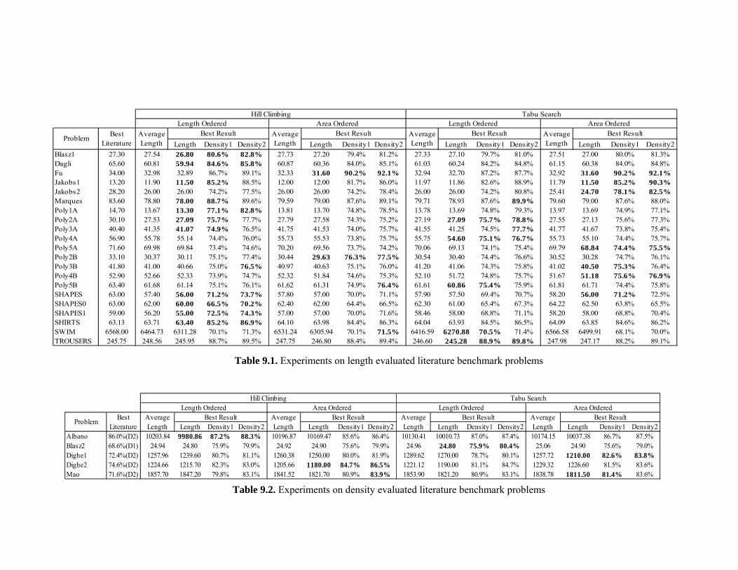
Le
ngth Dens y1 D sity227.30 27 4 6.80 80.6 8 8% 27.7365.60 60 1 9.94 84.6 8 8% 60.8734.00 32 8 2.89 86. 1% 32.3313.20 11 0 1.50 85.2 5% 12.0028.20 26 0 6.00 74. 5% 26.0083.60 78 0 8.00 88.7 6% 79.5914.70 13 7 3.30 77.1 8 8% 13.8130.10 27 3 7.09 75.7 7% 27.7940.40 41 5 1.07 74.9 5% 41.7556.90 55 8 5.14 74. 0% 55.7371.60 69 8 9.84 73. 6% 70.2033.10 30 7 0.11 75. 4% 30.4441.80 41 0 0.66 75. 7 5% 40.9752.90 52 6 2.33 73. 7% 52.3263.40 61 8 1.14 75. 1% 61.6263.00 57 0 6.00 71.2 7 7% 57.8063.00 62 0 0.00 66.5 7 2% 62.4059.00 56 0 5.00 72.5 7 3% 57.0063.13 63 1 3.40 85.2 8 9% 64.10568.0 646 73 11.28 70. 3% 6531.245.75 24 56 45.95 88. 5% 247.7
m Best teratu
Hill C mbingLengt Order
Av age Len th
Best R ult AveraLengtit en Len y s gt ensity1 ty Length Density1 Density2
Blasz1 .5 2 % 2. 27. % .2 10 79.7% % 27.51 27.00 80.0% 81.3%Dagli .8 5 % 5. 60. % .1 24 84.2% % 61.15 60.38 84.0% 84.8%Fu .9 3 7% 89. 31.60 % .1 70 87.2% % 32.92 31.60 90.2% 92.1%Jakobs1 .9 1 % 88. 12.00 % .0 86 82.6% % 11.79 11.50 85.2% 90.3%Jakobs2 .0 2 2% 77. 26.00 % .4 00 74.2% % 25.41 24.70 78.1% 82.5%Marques .8 7 % 89. 79.00 % .1 93 87.6% % 79.60 79.00 87.6% 88.0%Poly1A .6 1 % 2. 13.70 % .5 69 74.8% % 13.97 13.69 74.9% 77.1%Poly2A .5 2 % 77. 27.58 % .2 0 75.7% % 27.55 27.13 75.6% 77.3%Poly3A .3 4 % 76. 41.53 % .7 25 74.5% % 41.77 41.67 73.8% 75.4%Poly4A .7 5 4% 76. 55.53 % .7 6 75.1% % 55.73 55.10 74.4% 75.7%Poly5A .9 6 4% 74. 69.56 % .2 13 74.1% % 69.79 68.84 74.4% 75.5%Poly2B .3 3 1% 77. 29.63 % .5 40 74.4% % 30.52 30.28 74.7% 76.1%Poly3B .0 4 0% 6. 40.63 % .0 06 74.3% % 41.02 40.50 75.3% 76.4%Poly4B .6 5 9% 74. 51.84 % .3 72 74.8% % 51.67 51.18 75.6% 76.9%Poly5B .6 6 1% 76. 61.31 % .4 8 75.4% % 61.81 61.71 74.4% 75.8%SHAPES .4 5 % 3. 57.00 % .1 50 69.4% % 58.20 56.00 71.2% 72.5%SHAPES0 .0 6 % 0. 62.00 % .5 00 65.4% % 64.22 62.50 63.8% 65.5%SHAPES1 .2 5 % 4. 57.00 % .6 00 68.8% % 58.20 58.00 68.8% 70.4%SHIRTS .7 6 % 6. 63.98 % .3 93 84.5% % 64.09 63.85 84.6% 86.2%SWIM 6 0 4. 63 1% 71. 24 6305.94 % .5 6 0. 70.5% % 66.58 6499.91 68.1% 70.0%TROUSERS 8. 2 7% 89. 5 246.80 % .4 2 2 88.9% % 247.98 247.17 88.2% 89.1%
ProbleLi re
lih ed A rd
erg
es ge h
Be u
Tab rchng dered Area Ordered
A e Le
st Result verage ength
Best Resultgth Densit 1 Den ity2 Len h D20 79.4 81 % 27.33 27.36 84.0 85 % 61.03 60.
90.2 92 % 32.94 32.81.7 86 % 11.97 11.74.2 78 % 26.00 26.87.6 89 % 79.71 78.74.8 78 % 13.78 13.74.3 75 % 27.19 27. 974.0 75 % 41.55 41.73.8 75 % 55.75 54. 073.7 74 % 70.06 69.
76.3 77 % 30.54 30.75.1 76 % 41.20 41.74.6 75 % 52.10 51.74.9 76 % 61.61 60. 670.0 71 % 57.90 57.64.4 66 % 62.30 61.70.0 71 % 58.46 58.84.4 86 % 64.04 63.70.1 71 % 416.59 627 8888.4 89 % 46.60 245. 8
rea O eredst Res lt
Le th Orverag
ngthBe
Densi 281.084.887.788.980.8
89.979.3
78.877.776.775.476.675.875.775.970.767.371.186.571.4 65
89.8
u Sea
AL
perime a b mark p eTable 9.1. Ex nts on length evaluated liter ture ench
robl ms
Lengt Dens y1 D ity286.0% 2) 1 03.84 9980.8 87. % 8 3% 10196.68.6% 1) 94 24.80 75. 9% 24.9272.4% 2) 1 7.96 1239. 80. 1% 1260.374.6% 2) 1 4.66 1215. 82. 0% 1205.671.6% 2) 1 7.70 1847. 79. 1% 1841.5
A erage ngth
Best sult AveragLength
Hill Cl bingLeng Order
BesLitera e h it ens Length D 1 y sity1 Den Length Density1 Density2
Albano (D 02 6 2 8. 87 10169.47 8 % 13 1 3 0% 87 15 10037.38 86.7% 87.5%Blasz2 (D 24. 9% 79. 24.90 7 % 24. 9% 80. 24.90 75.6% 79.0%Dighe1 (D 25 60 7% 81. 8 1250.00 8 % 89 7% 80 2 1210.00 82.6% 83.8%Dighe2 (D 22 70 3% 83. 6 1180.00 8 % 21 1% 84 2 1226.60 81.5% 83.6%Mao (D 85 20 8% 83. 2 1821.70 8 % 53 9% 83 8 1811.50 81.4% 83.6%
Problem e Best ResultvLe
Re e Best lt ern
esult
im Sth ed Area Order gth O d Area Ordered
t tur sity2
.4% 10174.4% 25.06.1% 1257.7.7% 1229.3.1% 1838.7
AveragLength
Tabu earch
ensity Densit 2 Length Den5.6% 86.4 10 0.41 0010.7 87.5.6% 79.9 96 24.80 75.0.0% 81.9 12 .62 1270.00 78.4.7% 86.5 12 .12 1190.00 81.0.9% 83.9 18 .90 1821.20 80.
Resu Av age Le gth
Best Red Len rdere
periments on si a e ark eprobl ms den ty ev luat d literature benchmTable 9.2. Ex
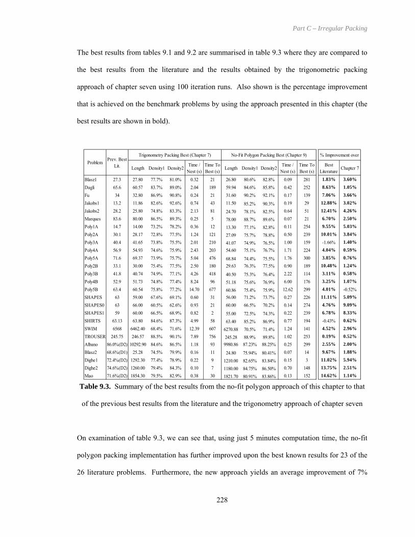
Part C – Irregular Packing
The best results from tables 9.1 and 9.2 are summ rised in table 9.3 where they are compared to
best results from the literature and the results obtained by the trigonometric packing
approach of chapter seven using 100 iteration runs. Also shown is the percentage improvement
that is achieved on the benchmark problems by using the approach presented in this chapter (the
best results are shown in bold).
a
the
Length Density1 Density2Time /
Nest (s) Best (s) Nest (s) Best (s) Literature
27.3 27.80 77.7% 81.0% 0.32 21 26.80 80.6% 82.8% 0.09 281 1.83%
Time To Length Density1 Density2
Time / Time To Best Chapter 7
Blasz1 3.60%
Dagli 65.6 60.57 83.7% 89.0% 2.04 189 59.94 84.6% 85.8% 0.42 252 8.63% 1.05%
Fu 34 32.80 86.9% 90.8% 0.24 21 31.60 90.2% 92.1% 0.17 139 7.06% 3.66%
1 0.19 29 12.88% 3.02%
s2 0.64 51 12.41% 4.26%
Marques 83.6 80.00 86.5% 89.3% 0.25 5 78.00 88.7% 89.6% 0.07 21 6.70% 2.50%
Poly2A 30.1 28.17 72.8% 77.5% 1.24 121 27.09 75.7% 78.8% 0.50 239 10.01% 3.84%
Poly4A 56.9 54.93 74.6% 75.9% 2.43 203 54.60 75.1% 76.7% 1.71 224 4.04% 0.59%
SHAPES0 63 66.00 60.5% 62.6% 0.93 21 60.00 66.5% 70.2% 0.14 274 4.76% 9.09%
SHAPES1 59 60.00 66.5% 68.9% 0.82 2 55.00 72.5% 74.3% 0.22 239 6.78% 8.33%
SHIRTS 63.13 63.80 84.6% 87.3% 4.99 58 63.40 85.2% 86.9% 0.77 194 -0.43% 0.62%
TROUSER
% Improvement overProblem
Prev. Best Trigonometry Packing Best (Chapter 7) No-Fit Polygon Packing Best (Chapter 9)
Jakobs 13.2 11.86 82.6% 92.6% 0.74 43 11.50 85.2% 90.3%Jakob 28.2 25.80 74.8% 83.3% 2.13 81 24.70 78.1% 82.5%
Poly1A 14.7 14.00 73.2% 78.2% 0.36 12 13.30 77.1% 82.8% 0.11 254 9.55% 5.03%
Poly3A 40.4 41.65 73.8% 75.5% 2.01 210 41.07 74.9% 76.5% 1.00 159 -1.66% 1.40%
Poly5A 71.6 69.37 73.9% 75.7% 5.04 476 68.84 74.4% 75.5% 1.76 300 3.85% 0.76%
Poly2B 33.1 30.00 75.4% 77.5% 2.50 180 29.63 76.3% 77.5% 0.90 189 10.48% 1.24%
Poly3B 41.8 40.74 74.9% 77.1% 4.26 418 40.50 75.3% 76.4% 2.22 114 3.11% 0.58%
Poly4B 52.9 51.73 74.8% 77.4% 8.24 96 51.18 75.6% 76.9% 6.00 176 3.25% 1.07%
Poly5B 63.4 60.54 75.8% 77.2% 14.70 677 60.86 75.4% 75.9% 12.62 299 4.01% -0.52%SHAPES 63 59.00 67.6% 69.1% 0.60 31 56.00 71.2% 73.7% 0.27 226 11.11% 5.09%
SWIM 6568 6462.40 68.4% 71.6% 12.39 607 6270.88 70.5% 71.4% 1.24 141 4.52% 2.96%
S 245.75 246.57 88.5% 90.1% 7.89 756 245.28 88.9% 89.8% 1.02 253 0.19% 0.52%
24.80 75.94% 80.41%
Albano 86.0%(D2) 10292.90 84.6% 86.5% 1.18 93 9980.86 87.23% 88.25% 0.25 299 2.55% 2.00%
Blasz2 68.6%(D1) 25.28 74.5% 79.9% 0.16 11 0.07 14 9.67% 1.88%
Dighe1 72.4%(D2) 1292.30 77.4% 78.9% 0.22 9 1210.00 82.65% 83.84% 0.15 3 11.02% 5.94%
Dighe2 74.6%(D2) 1260.00 79.4% 84.3% 0.10 7 1180.00 84.75% 86.50% 0.70 148 13.75% 2.51%
Mao 71.6%(D2) 1854.30 79.5% 82.9% 0.38 30 1821.70 80.91% 83.86% 0.13 152 14.62% 1.14%
Lit.
Table 9.3. Summary of the best results from the no-fit polygon approach of this chapter to that
of the previous best results from the literature and the trigonometry approach of chapter seven
On examination of table 9.3, we can see that, using just 5 minutes computation time, the no-fit
polygon packing implementation has further improved upon the best known results for 23 of the
26 literature problems. Furthermore, the new approach yields an average improvement of 7%
228
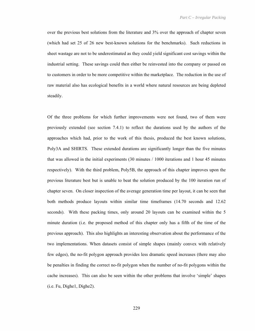
Part C – Irregular Packing
over the previous best solutions from the literature and 3% over the approach of chapter seven
(which had set 25 of 26 new best-known solutions for the benchmarks). Such reductions in
she the
dustrial setting. These savings could then either be reinvested into the company or passed on
in the use of
best known solutions,
oly3A and SHIRTS. These extended durations are significantly longer than the five minutes
s unable to beat the solution produced by the 100 iteration run of
chapter seven. On closer inspection of the average generation time per layout, it can be seen that
both methods produce layouts within similar time timeframes (14.70 seconds and 12.62
seconds). With these packing times, only around 20 layouts can be examined within the 5
minute duration (i.e. the proposed method of this chapter only has a fifth of the time of the
previous approach). This also highlights an interesting observation about the performance of the
two implementations. When datasets consist of simple shapes (mainly convex with relatively
few edges), the no-fit polygon approach provides less dramatic speed increases (there may also
be penalties in finding the correct no-fit polygon when the number of no-fit polygons within the
cache increases). This can also be seen within the other problems that involve ‘simple’ shapes
(i.e. Fu, Dighe1, Dighe2).
et wastage are not to be underestimated as they could yield significant cost savings within
in
to customers in order to be more competitive within the marketplace. The reduction
raw material also has ecological benefits in a world where natural resources are being depleted
steadily.
Of the three problems for which further improvements were not found, two of them were
previously extended (see section 7.4.1) to reflect the durations used by the authors of the
approaches which had, prior to the work of this thesis, produced the
P
that was allowed in the initial experiments (30 minutes / 1000 iterations and 1 hour 45 minutes
respectively). With the third problem, Poly5B, the approach of this chapter improves upon the
previous literature best but i
229

Part C – Irregular Packing
However, the benefit of the no-fit polygon is shown in the benchmark problems that have been
taken from the textile industry. For example, for the problems Marques and Mao, layouts are
generated three times as quickly
230
as the trigonometry approach. With Albano and Dagli there is a
fourfold increase in nesting speed, SHIRTS and TROUSERS are both seven times quicker and,
finally, layouts for the SWIM dataset (consisting of very complex pieces) can be produced in a
tenth of the time that is required by the trigonometry based approach. Therefore it can be seen
that the no-fit polygon provides the greatest speed improvements for the problems that contain
highly irregular shapes or shapes that are created from many primitives. However, on the
problems involving simple shapes (some of which have been identified) the no-fit polygon
yields speed improvements, albeit less dramatic. These speed increases can be used to exam
more of the search space (as successfully onstrated with the presented method) or it
provide the necessary additional speed to allow more complicated packing strategies to be
developed.
Referring back to the experiments of chapter seven (using the trigonometric implementation),
the literature benchmark problems that were not improved upon in the first set of experim
were extended to allow the same time as reported by the authors who produced the best-known
solutions (section 7.4.1). These problem
which were extended to allow durations of 551.73s, 2019.77s, 6367.57s and 13613.67s
respectively. Two other problems, SHAPES0 and Poly3A, were extended to allow 10,000
iterations as run times were not provided. This yielded new best solutions for five of these six
problems (all except SHAPES0). Table 9.4 compares the previous best-known solutions for
these problems and the solutions generated from the new approaches presented in this thesis.
Once again, the best solutions are shown in bold typeface.
still
ine
may
ents
dem
s were Blasz1, SHAPES1, SHIRTS and TROUSERS
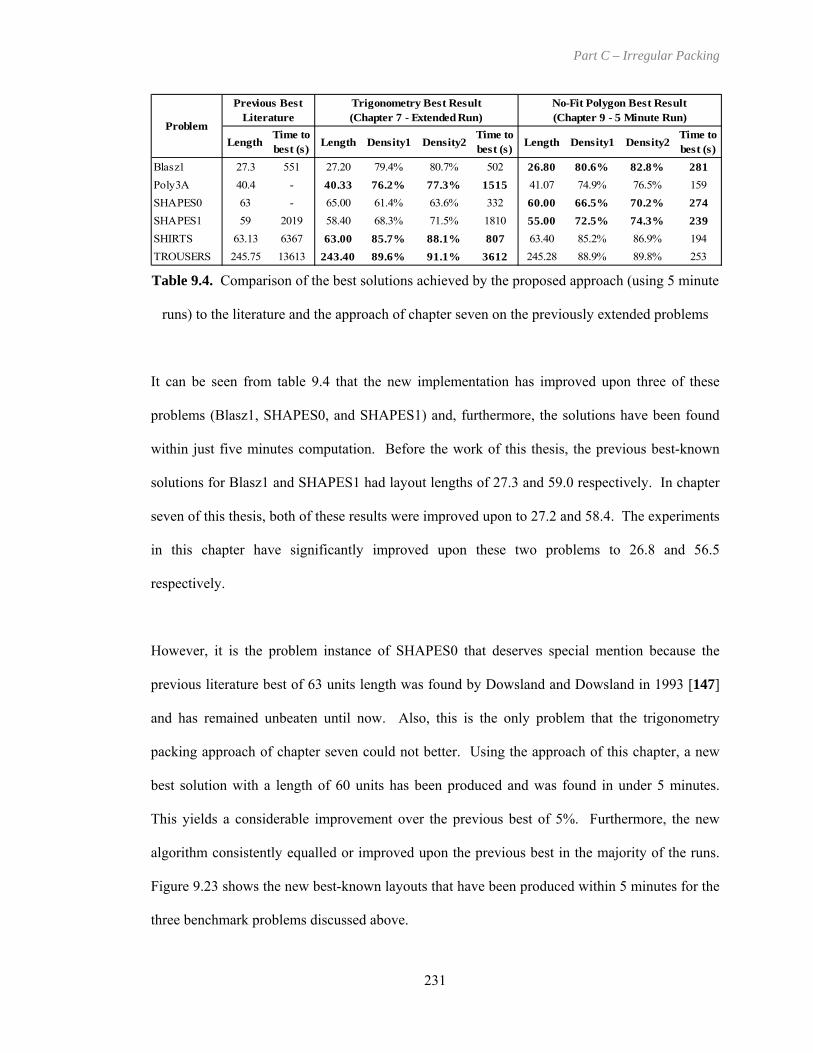
Part C – Irregular Packing
LengthTime t
Problemo
best (s) Length Density1 Density2Time to best (s) Length Density1 Density2
Time to best (s)
Poly3A 40.4 - 40.33 76.2% 77.3% 1515 41.07 74.9% 76.5% 159
SHAPES1 59 2019 58.40 68.3% 71.5% 1810
Trigonometry Best Result (Chapter 7 - Extended Run)
No-Fit Polygon Best Result (Chapter 9 - 5 Minute Run)
Previous Best Literature
Blasz1 27.3 551 27.20 79.4% 80.7% 502 26.80 80.6% 82.8% 281
SHAPES0 63 - 65.00 61.4% 63.6% 332 60.00 66.5% 70.2% 27455.00 72.5% 74.3% 239
SHIRTS 63.13 6367 63.00 85.7% 88.1% 807 63.40 85.2% 86.9% 194TROUSERS 245.75 13613 243.40 89.6% 91.1% 3612 245.28 88.9% 89.8% 253
Table 9.4. Comparison of the best solutions achieved by the proposed approach (using 5 minute
It can be seen from table 9.4 that the new implementation has improved upon three of these
within just five minutes computation. Before the work of this thesis, the previous best-known
solutions for Blasz1 and SHAPES1 had layout lengths of 27.3 and 59.0 respectively. In chapter
seven of this thesis, both of these results were improved upon to 27.2 and 58.4. The experiments
in this chapter have significantly improved upon these two problems to 26.8 and 56.5
respectively.
previous literature best of 63 units length was found by Dowsland and Dowsland in 1993 [147]
and has remained unbeaten until now. Also, this is the only problem that the trigonometry
best solution with a length of 60 units has been produced and was found in under 5 minutes.
This yields a considerable improvement over the previous best of 5%. Furthermore, the new
algorithm consistently equalled or improved upon the previous best in the majority of the runs.
three benchmark problems discussed above.
runs) to the literature and the approach of chapter seven on the previously extended problems
problems (Blasz1, SHAPES0, and SHAPES1) and, furthermore, the solutions have been found
However, it is the problem instance of SHAPES0 that deserves special mention because the
packing approach of chapter seven could not better. Using the approach of this chapter, a new
Figure 9.23 shows the new best-known layouts that have been produced within 5 minutes for the
231

Part C – IrregulPart C – Irregular Packing
i)
)
Figure 9.23. New bes
(Length = 2
9.3.2 Extended Exp
he next set of experim
ngth and area initial
hilst the proposed
ROUSERS dataset (
length measures to th
0.003%). However, th
better than the average
T
seven. The presented
runs and, therefore, o
10 runs were allowed
le
W
T
i
ii232
t layouts for previously extend
6.8), ii) SHAPES0 (Length =
eriments on the Literature B
ents involved extending the s
orderings. The best and avera
approach has only produce
see figure 9.24), the solution
e best solutions of chapter se
e average solutions produced
s of chapter seven for all three
approach has already improv
nly Poly3A, SHIRTS and TRO
for each problem using both h
ii)
ed literature benchmark problems: i) Blasz1
60), iii) SHAPES1 (Length = 55)
enchmarks
ame problems that were extended in chapter
ith decreasing
ge solutions are presented in table 9.5.
d one new best-known solution for the
s for the other two problems have similar
ven (both Poly3A and SHIRTS are within
by the proposed approach of this chapter are
of the problems.
ed upon three of these during the 5 minute
USERS have been extended. Once again,
ill climbing and tabu search w

Part C – Irregular Packing
Length Time to best (s) Length Density1 Density2 Time to
best (s) Length Density1 Density2 Time to best (s)
Poly3A 40.40 - 41.45 40.33 76.2% 77.3% 1515 40.95 40.45 76.0% 78.1% 429
SHIRTS 63.13 6368 63.66 63
TROUSERS 245.75 13614 246.40 243.
.00 85.7% 88.1% 807 63.61 63.16 85.5% 87.9% 806
40 89.6% 91.1% 3612 244.10 243.00 89.8% 90.8% 12484
No-Fit Polygon Best Result (Chapter 9)
Avr Length
Best Solution
ometry Best Result (Chapter 7)
Length
Best SolutionProblem
Trigon
Avr
Previous Literature Best
Table 9.5. Extended experiments with the no-fit polygon packing approach
Figure 9.24. New best layout for TROUSERS data (Length = 243.0, Density1 = 89.8%)
9.3.3 Experiments on the New Benchmark Problems (Profiles1 – Profiles10)
Finally, experiments were conducted on the new benchmark problems that were introduced in
chapter seven of this thesis (see section 7.3). For these problems, 10 runs were conducted with
both hill climbing and tabu search (with both length and area sorted orderings) where each run
was allowed 30 minutes computation time. These experiments have been repeated using the
packing approach presented within this chapter and the results are presented in table 9.6. The
best results are summarised in table 9.7 (best results are shown in bold).
These experiments have produced new best solutions for 7 of the 10 datasets. For the datasets in
which the new approach did not achieve improvements over chapter seven, solutions were only
slightly worse (within 1%).
233

L
engt De sity1 Dens 2 Le thiles1 138 14 1380.1 6% 83. 391.40 13 .00iles2 326 10 3216.0 0% 50. 230.98 31 19iles3 807 88 881. 5 9% 54.0 230.33 81 .66iles4 247 46 2452.4 2% 75. 475.58 24 .35iles5 339 32 3367.8 4% 70. 401.17 33 94iles6 313 01 121. 7 0% 78.6 172.97 31 .02iles7 130 78 292. 7 4% 79.9 307.44 12 30iles8 130 17 1268.9 8% 79. 283.19 12 .98iles9 131 73 278. 5 7% 54.2 298.42 12 .00iles10 113 .40 219. 6 8% 66.6 515.0 114 99
blem
H Clim ngLeng h Ord d rea O
Av ge Len th
Bes Resul veragngthh n ity ng y1 Den h en ity n y ensity2
Prof 9. 0 81. 0% 1 86 % 82. 2. 0 80. % 1 9 % 84.5%Prof 2. 6 50. 8% 3 94. % 51. 4. 0 49. % 3 23 % 50.8%Prof 3. 7 13 2. % 8 89 % 51. 4. 4 52. % 8 45 % 53.0%Prof 6. 2 75. 7% 2 64 % 75. 6. 2 6 6. % 2 82 % 74.8%Prof 4. 8 69. 6% 3 51. % 70. 5. 5 69. % 3 84 % 70.4%Prof 4. 3 36 5. % 3 56 % 75. 1. 6 74. % 3 61 % 76.3%Prof 5. 1 30 7. % 1 92. % 79. 6. 0 77. % 1 09 % 79.6%Prof 3. 8 78. 8% 1 68 % 79. 8. 8 77. % 1 3 % 82.1%Prof 4. 1 21 2. % 1 90 % 53. 8. 2 51. % 1 92 % 53.3%Prof 73 11 60 5. % 11 3 03. % 65.4% 2 1 50 65. % 11 0 8 % 64.7%
ProB suB sult a
gt A e
Le
ill bi a art ere A rd t ere A rd
erag
t t A e Le sity2 Lengt D sity1 Dens 2 Le gth Densit 1 D
5% 141 88 1404.8 2% 81.4 394.54 135 .90 82.85% 326 40 3252.7 4% 50.3 267.78 32 .30 49.87% 807 34 7999.7 1% 53.0 177.60 80 .84 51.84% 246 55 425.2 7 0% 76.5 486.49 24 .72 74.28% 338 32 3364.3 5% 70.5 399.48 33 .90 69.16% 316 51 3146.5 4% 76.8 176.52 31 .22 74.19% 131 32 1296.3 1% 77.7 313.44 13 .10 76.48% 130 61 1293.8 3% 77.5 285.44 126 .11 79.12% 130 93 1298.6 9% 52.9 303.43 12 .63 52.1
1139 .36 1302. 3% 66.0 653.4 115 5.81 63.7
est Re ltAver ge Len th
Bes Result veragngth
T bu Se chLeng h Ord d rea O ered
Densit81.350.350.974.869.874.277.478.852.264.8
est Reered
Table 9.6. E ri ts on new be ark problem
xpe men nchm s
Le gth Den y1P files1 74 82.P files2 10 50.P files3 89 50.P files4 12 75.P files5 70 70.P files6 86 75.P files7 30 77.P files8 70 75.P files9 67 53.Pr files1 10 66.
st So tion
T gono etry A proacChapt r 7)
P oblem
n sit D y2 Length s tyro 1377. 0% 1359.90 .8 % %ro 3216. 0% 3194.19 .3 % %ro 8193. 9% 7881.13 .9 % %ro 2453. 1% 2425.26 .0 % %ro 3332. 2% 3351.94 .8 % 8ro 3097. 6% 3121.36 .0 % 6ro 1296. 1% 1292.30 .4 % %ro 1318. 8% 1263.11 .1 % %ro 1290. 1% 1278.21 .7 % %o 0 11160. 2% 66.8% 11219.60 .8 % 3
P tIm e
erte
No-Fit Po oa stpt
Be lu B o
ri m p h ( e
r
Den ity1 Densi 282 % 85.4 1.2950 % 51.5 0.6852 % 54.0 3.8276 % 76.5 1.1469 % 70.8 -0.5 %75 % 78.6 -0.7 %77 % 79.9 0.3179 % 82.1 4.2252 % 54.2 0.9765 % 66.6 -0.5 %
ercen age prov ment
ov Chap r 7
lygon Appr ch Be (Cha er 9)est S lution
ensit85.2%51.3%52.6%75.7%73.6%77.8%80.2%77.2%54.9%
Best
Table 9.7. S f best results for n e mark problemew b nch summary o

9.4 Summary
he aim of this chapter was to develop a no-fit polygon packing algorithm that could be used
previously discussed, the fast and efficient handling
as investigated through repeated experiments on the literature benchmark
roblems and the new datasets. The packing approach yielded an average improvement in
and an average
T
within industrial settings. However, as has
of shapes containing both holes and arcs has been an underlying feature of this work. Therefore,
in the first part of the chapter, an algorithm was presented that can robustly generate no-fit
polygons for shapes, which may also consist of arcs, through extension of the previous no-fit
polygon generation algorithm of chapter eight. This is a significant milestone for the academic
community as there have not been any published approaches which address no-fit polygon
generation with shapes involving arcs. In the second part of the chapter, the packing approach
of chapter seven was reimplemented to utilise the arc/line no-fit polygon for the detection and
resolution of overlaps. The performance of the no-fit polygon based implementation of the
packing algorithm w
p
solution quality of 7% over the previous best solutions from the literature
improvement of 3% was achieved over the packing method presented within chapter seven
(which had, itself, produced the best known results for 25 of the 26 literature benchmark
problems). The presented packing approach of this chapter was able to achieve new best-known
solutions for 30 of the 36 benchmark problems (including a 5% improvement for the SHAPES0
problem which could not be improved upon by the packing approach of chapter seven).
Therefore, the two irregular packing approaches of this thesis have produced the best-known
solutions for all 26 of the literature benchmark problems. The approach also improved upon 7
of the 10 new benchmark datasets which contain shapes with lines, arcs and holes. The
additional speed gain from use of the no-fit polygon enables more layouts to be examined in less
computational time which, on average, allows for higher quality solutions to be obtained. These
features make the presented packing approach a strong candidate for use in the industrial setting.
235

Part D –Discussion
PAR T D – DISCUSSION
In Part B and Part C, new strategies for automating layout generation for the rectangular and
irregular variants of the two-dimensional packing problem were presented. The purpose of this
part of the thesis is to draw conclusions and to analyse the presented work, to discuss the future
research direction that could be undertaken and to show how the work has been disseminated.
Chapter ten provides a summary of the research conducted within this thesis and places it in
context to the field of cutting and packing, conclusions are drawn for the developed approaches
presented within this thesis and the possible future research direction that could be followed in
rder to improve or extend this work.
Chapter eleven provides an insight into why this work has been of significant benefit to both the
o
academic community and the industrial partner. Finally, the chapter presents an overview of the
commercialisation opportunities that have arisen as a direct result of this research.
236

Part D –Discussion
CHAPTER TEN
Conclusions
This thesis has provided several milestones for two-dimensional cutting and packing problems.
The main contributions of this thesis are summarised below giving particular attention to the
context of the work related to the previous literature.
10.1.1 Development of a New Fast and Effective Rectangle Packing Heuristic
The rectangul
10.1 Discussion
ar variant of the packing problem benefits from simpler implementation than the
of each shape is known and, therefore, specialised intersection
detection loyed. However, the show be NP-
Complete [15]. The best performing placement heuristics, prior to this thesis, have been
ottom-left-fill style algorithms. These operate by firstly sorting the rectangles into some order
revious state-of-the-art algorithms because
irregular variant because the form
routines can be emp problem has still been n to
b
(usually by decreasing height or decreasing width) and then placing each rectangle as close to
the bottom left corner of the sheet as possible. In order to fill holes, a list of potential placement
locations must be maintained and intersection testing must be performed between the rectangles
already assigned to the sheet and the current rectangle being placed. Both of these operations
can be expensive when the problem size becomes large. The bottom-left-fill algorithms
generally produce better results when hybridised with metaheuristics to generate different input
orderings that can then be evaluated. One of the first contributions of this work was the
development of a fast rectangle placement heuristic that is based on the principles of best-fit.
This is a completely different methodology to the p
237

Part D –Discussion
the list of available rectangles is examined at each placement step and the best-fitting rectangle
n dynamically. A novel method of representing the available sheet space is presented is chose
using the height profile of the layout. This representation, along with the best-fit method,
of the material required to fulfil an order is necessary to
rovide a competitive quotation).
ttom-left-fill algorithms produce
xcellent layouts on small problems as they can search many potential arrangements. It is
intuitive that the metaheuristic bottom-left-fill approach can be applied to the latter rectangles of
the solution produced by the best-fit heuristic. It has been shown that this approach makes
enables the heuristic to produce a layout very quickly because holes are never created unless
absolutely necessary and intersection testing is redundant (unlike the previous algorithms). The
algorithm produces solutions that are much denser (lower overall height required) than the other
approaches from the literature for medium and large problem instances and, furthermore, are
produced within just a few seconds. Although subsequent algorithms proposed in this thesis
have produced better solutions than the best-fit heuristic, the speed of the approach would allow
it to be employed where real-time packing is required such as dynamic problems (whereby new
orders arrive periodically and layouts should be repacked to include any new data) or online
quoting systems (whereby an indication
p
10.1.2 Hybridisation of Two Packing Algorithms to Combine Relative Strengths
A further contribution of this thesis is the hybridisation of the best-fit heuristic with the
metaheuristic bottom-left-fill placement heuristic method. The author believes this to be one of
the first approaches to combine the relative strengths of two separate packing algorithms to
generate layouts of a better quality than either of the constituent methods. It was emphasised
that the best-fit heuristic can produce extremely dense solutions at the start of packing when
there is a large selection of rectangles from which to choose. However, after placing the
majority of the rectangles, there is inevitably a smaller selection and therefore more wastage
occurs at the top of layouts. Conversely, the metaheuristic bo
e
238

Part D –Discussion
significant improvements over the best-known solutions on all of the benchmark problems of the
one minute of computation time.
ach further
proves on the newly presented rectangle packing algorithms within this thesis (which, as
oved on all benchmarks from the literature). However, the
0.1.4 Presentation of a New Placement Technique for Irregular Packing
s to rectangle packing,
literature using, in general, just
10.1.3 Introduction of User Interaction
A method is also presented to allow the user to interact with the algorithms by identifying poor
regions within the layout. The metaheuristic bottom-left-fill algorithm can then be invoked to
target the rectangles within the identified regions. The user interaction appro
im
stated above, have already impr
method requires more computational time due to the interactivity and obviously requires a
human operator to oversee the procedure. To the author’s knowledge, this is the first time that
user-interactive approaches have been evaluated using such a wide range of benchmark data
from the literature.
1
The irregular variant of the packing problem involves similar objective
that is to minimise the total length of sheet required and, as mentioned previously, the irregular
variant of the problem involves significantly more complex geometric modelling, which yields
its own difficulties. This thesis contributes a new heuristic algorithm which, through the use of
overlap resolution in the vertical axis, generates significantly better results than the previous
state-of-the-art on a wide range of established benchmark problems. The developed algorithm is
not only able to pack shapes involving the traditional line polygonal representation but can also
pack shapes that incorporate circular arcs and holes. This in itself represents a significant
improvement over the previous state-of-the-art. In general, an average improvement of 5% is
achieved over previous methods and solutions are produced within quick timeframes (5 minutes
for the majority of problems).
239

Part D –Discussion
10.1.5 Development of a Complete and Robust Algorithm for Generation of No-Fit
Polygons involving Non-Convex Polygons
The no-fit polygon defines the intersection relationship between pairs of shapes and is
considerably faster than its trigonometric counterpart. For this reason, there has been
considerable interest in using the no-fit polygon for automated packing. However, the
generation of the no-fit polygon becomes complicated in all but the simplest convex shape case
and previous generation algorithms for non-convex shapes have reported degenerate cases for
which the algorithms cannot derive the complete no-fit polygon. The author feels that one of the
major milestones that has been provided to the academic community through this research
programme has been the development of a complete and robust algorithm for calculating the no-
fit polygon between pairs of shapes. As this algorithm can generate no-fit polygons (for all of
e degenerate cases including shapes with holes) robustly and quickly, it offers significant
r g within an industrial setting.
th
comme cial advantages for faster automated packin
10.1.6 Modification of the No-Fit Polygon Generation Algorithm to Allow Shapes
Containing Arcs
In addition to presenting the first no-fit polygon not to suffer from degeneracies, large steps have
been taken into producing an arc-capable no-fit polygon algorithm through the modification of
the line based algorithm. Using the property that the no-fit polygon of two circles is also a
circle, it was shown how arcs create a section of the circular no-fit polygon (defined by tangent
points).
There have not been any previous attempts to generate no-fit polygons for shapes containing
arcs and the author considers this to be an important development for both industrial and
academic study.
240

Part D –Discussion
10.1.7 Identification of No-Fit Polygon Properties and Applicability of Caching within the
Generation Process for Packing Problems
In order to use the faster no-fit polygon based intersection during the packing phase, no-fit
olygons must be generated for all pairs of shapes. In normal circumstances, (nm)2 no-fit
s and m is the number of
p
polygons must be generated (where n is the number of unique shape
rotations). This generation procedure can be expensive and results in significant memory
overheads for larger problems. For example, with sixteen different shapes and 90° rotations
(four rotations: 0°, 90°, 180°, 270°), (4*16)2 = 4096 no-fit polygons must be produced. This
thesis identifies the rotational properties of no-fit polygons and shows that a reduction in the
number required can be achieved. The proposed method of reduction would result in only 408
no-fit polygons being generated in the example given above (as opposed to 4096 without
reductions). The reduced number of no-fit polygons that must be generated is generalised in
equation (1).
Number of NFPs = ( )
⎟⎟⎞
⎜⎜⎛
⎥⎥⎤
⎢⎢⎡ +
⎟⎠⎞
⎜⎝⎛ +
21
21 mnn
where n > 0, m > 0 (1) ⎠⎝
The possibility of reductions has not been reported previously in the literature and, thus, is
included in this work. Further to this, a modified version of the irregular packing technique
(discussed in 10.1.3 above) is presented that utilises the faster no-fit polygon intersection testing
during the nesting process. Although the packing algorithm is fundamentally the same, the
introduction of the no-fit polygon produces faster layouts and yields considerable time savings
which can be used to evaluate more of the problem search space. This is reflected in the quality
of solutions that are produced which are better than any other reported method within the
literature and the other trigonometric irregular packing implementation presented in chapter
seven of this thesis (and discussed in 10.1.3 above).
241

Part D –Discussion
10.1.8 Generation of the Best-Known Solutions for 60 Benchmark Datasets (Both
et, SHAPES0, has not been improved upon for over ten years
ut the no-fit polygon packing approach of chapter nine yields an improvement of around 5%
literature best
enchmarks are of particular interest as they present shapes
at have not been represented previously within the literature. Namely, the new benchmarks
l setting and consist of shapes
Rectangular and Irregular) Gathered from over Twenty Years in Cutting and
Packing Research
The techniques presented within this thesis have produced the best-known results for all of the
sixty benchmark problems that are readily available within the literature for both rectangular and
irregular packing. These datasets have been taken from over twenty years of cutting and
packing literature involving some invented problems and some problems that are drawn from
the textile industry. As a particular example of the advances that the new algorithms provide,
the solution to one irregular datas
b
over the previous best and consistently obtains better layouts than the previous
within three minutes of execution time.
10.1.9 Introduction of New Benchmark Problem Instances to the Literature
Twenty-eight new rectangle benchmark problems have been produced and provided to the
academic community. In addition to this, ten new benchmark problems for irregular packing
have been presented. The irregular b
th
include irregularities that are commonplace within the industria
that not only contain lines but arcs and holes as well. The author hopes that the introduction of
these new benchmark problems will facilitate greater research into the areas of rectangular and
irregular packing and, in the latter case, will promote the use of more typical shapes, containing
arcs and holes, which occur frequently in the industrial setting.
242

Part D –Discussion
10.2 Future Wo
This research programme has been very successful in producing state-of-the-art packing
algorithms and has achieved the best-known solutions on all of the readily available benchmark
problems from the literature. However, the author believes several modifications to this work
may yield further improvements in performance (both in the quality of solutions produced and
the time required to achieve them). The author is currently pursuing the following:
10.2.1 Algorithmic Analysis
Although the algorithms presented within this thesis have produced excellent layouts in very
quick time on a wide range of existing literature benchmark problems, it was beyond the scope
of this PhD programme to provide full algorithmic complexity analyses. However, it is
recognised that this represents an interesting future research direction to further investigate these
algorithms and to define what is and is not possible computationally in the best and worst cases.
10.2.2 Problem Categorisation and Automatic Algorithm Selection
One area that has not been explored within this work is the categorisation of problems.
Fundamentally, it could be said that the problems used within this thesis have been manually
categorised into rectangular and irregular data with different algorithms being applied to these
types. However, further benefits might be achieved through automatic categorisation and
statistical analysis of input data before an approach is selected from a suite of different packing
algorithms. As an example, assume we have some data which we analyse and find to contain
only rectangles. In such instances, we know that there are good packing algorithms to tackle
this data (i.e. the best-fit heuristic or metaheuristic bottom-left-fill approaches). An indication of
problem size should also be considered (e.g. the best-fit heuristic was found to perform the best,
in general, for problems involving 50 or more rectangles). Other data characteristics may also
rk
243

Part D –Discussion
influence the choice of one algorithm over another such as the distribution of rectangle sizes
(maybe there are only a few distinct sizes of rectangle but with m
further example, assume we have some irregular data tain any shape). Analysis of
the data may show that there are a number of rectangles, circles and unidentified shapes. In
such instances, several algorithms that are tailored to specific data may be used to produce the
overall layout (perhaps the best-fit heuristic algorithm the rectangles then a circle
packing approach for the circular objects and finally the packing approach of chapter nine). In
addition to t different
earch algorithms (and search parameters) perform better on certain types of data and this would
e informed automatic selection of
e main features of a
yperheuristic is that there is a layer of abstraction between the hyperheuristic and the problem
bstraction means that the
nsive methods and may
deliver better average and worst-case performance than other heuristic methods. Hyperheuristic
approaches have already been successfully applied to bin packing in Ross et al. (2002) [261] and
ultiple instances of each). As a
(i n.e. can co
to pack
the automatic selection of packing algorithms, it may also be the case tha
s
also be an interesting avenue for further investigation. Th
algorithms and search parameters should allow for better layouts to be produced.
10.2.3 Hyperheuristics and Packing Problems
Hyperheuristics are a new search paradigm for solving optimisation problems and can be
thought of as heuristics that choose low-level heuristics [259,260]. One of th
h
domain (and related low-level heuristics). This layer of a
hyperheuristic cannot utilise any domain specific information (unlike other specific solution
approaches) and, instead, may only use general domain-independent feedback from the search to
guide low-level heuristic selection (e.g. improvement in evaluation, time taken, recently
employed heuristics, good sequences of heuristics). This maintains the generality of the
hyperheuristic which enables it to be transferred and applied across a wide range of optimisation
problems without change. Therefore, hyperheuristic methods will be appreciably cheaper in
terms of implementation costs and easier to use than knowledge-inte
244

Part D –Discussion
subsequently in Ross et al. (2003) [262]. Therefore, it would be an interesting extension to
apply and evaluate hyperheuristic approaches on the two-dimensional packing problems that
have been addressed within this thesis.
10.2.4 Automatic Identification of Poor Regions within a Layout
In chapter four, the best-fit heuristic was hybridised with a metaheuristic bottom-left-fill
method. This involved packing the first n rectangles with the best-fit heuristic and then allowing
the metaheuristic bottom-left-fill method to produce good layouts with the remaining rectangles.
It was shown that this outperforms both of the constituent algorithms but requires the pre-
specification of the number of rectangles to pass to the metaheuristic bottom-left-fill phase.
However, because different problems can have vastly different characteristics, an interactive
approach was developed to allow users to target the metaheuristic bottom-left-fill at the poorer
regions of a layout (thus removing the need for pre-specification of the num er of rectangles to
be passe through
the user interaction method achieved significant benefits in solution quality it has two
drawbacks: i) the approach can require longer computational time due to requiring feedback
from the user and, more importantly, ii) the approach requires a human operator. If we could
develop algorithms to detect poorer regions within layouts then both pre-specification and the
user can be removed from the system. This has benefits because the algorithms can then operate
out of working hours (i.e. overnight). Thus, the algorithm can use longer durations and this
alone should facilitate better quality solutions.
b
d to the metaheuristic bottom-left-fill phase). Although the solutions produced
245

Part D –Discussion
10.2.5 Applying Similar User Interaction Models to Irregular Packing
One improvement that could be advantageous for irregular packing is the provision of a similar
user interaction procedure as was developed for the rectangle packing approach of chapter five.
packing approaches operate by decoding piece orderings,
the presented user interaction method can be directly applied to irregular packing without
0.2.6 Extension of Arc No-Fit Polygon Generation to Include Start Points
In chapter nine, the complete and robust line no-fit polygon generation algorithm from chapter
eight was extended to allow shapes containing arcs. Although this is the first time any no-fit
general, the space is more difficult to utilise). We can see that this is also
entified by a large fluctuation in the path of the no-fit polygon (i.e. a ‘sharp’ concavity).
As both the rectangular and irregular
change (the user selects poor quality regions or clusters of shapes which are then removed and
repacked in different combinations whilst unselected shapes remain fixed). The author expects
similar improvements in solution quality to be achieved for the irregular packing as was
achieved with rectangle packing.
1
polygon approach has attempted shapes containing arcs, the idea of start points (presented in
section 8.3) must be extended to ensure no-fit polygon completeness. The extension of start
points to arcs requires similar concepts to that provided in chapter nine and the author is
currently pursuing this development.
10.2.7 Preprocessing into Clusters using the No-Fit Polygon
In this thesis, the no-fit polygon was identified as a geometric tool for faster detection and
resolution of overlapping shapes. However, analysis of the no-fit polygon may also be
beneficial for the pre-clustering of shapes. For example, figure 10.1 revisits the no-fit polygon
of two shapes from the SWIM dataset, it can be seen that the most efficient clustering of these
two shapes occurs when one shape is placed inside the other shape’s concavity (it is beneficial to
fill concavities as, in
id
246

Part D –Discussion
Figure 10.1. Clustering potential of no-fit polygons
If this fluctuation can be detected algorithmically, we can cluster a large proportion of the
permutation approaches (such as the
ones presented in this thesis).
10.2.8 Development of More Intelligent Packing Algorithms
The irregular packing approaches developed w bottom-
left packing shape in its
leftmost position on the sheet. However, this may not always be the best policy. For example,
take the shape of figure 10.1 that contains the concavity and assume that it may be placed in
either its 0° or 180° orientation (with concavity facing left or right respectively). Generally, it is
better to face concavities to the right (i.e. facing the open sheet) as a left facing concavity
becomes ‘clo pace within
the concavity
orientations orientations
can be place hape is placed in its
less desirable orientation (left-facing
the shape. ents as the
concavity’s space can be exploited by more shapes (i.e. the other shape from figure 10.1).
shapes before packing commences. A nesting algorithm would then treat these clusters as a
single shape which would reduce the search space for shape
ithin this thesis follow the well-known
methodology. This involves a greedy placement heuristic that places a
sed’ (i.e. a hole) which limits the number of shapes that can utilise the s
. Figure 10.2 shows the leftmost position of the example shape in each of its
in a typical packing scenario. In figure 10.2 we can see that the two
d at almost the same position along the x axis. However, the s
concavity) because it is marginally the leftmost position for
In this instance, the other position may allow for better future placem
247

Part D –Discussion
Figure 10.2. Greedy leftmost placement and a better placement position
10.2.9 Dynamic Layout Analysis and Online Clustering
Leftmost
Position
Position
Placement
Better Placement
(Potentially)
During the packing stages, a considerable amount of information is created about the positional
relationships of groups of shapes. However, in the current packing model, this information is
not exploited. One possible extension for the developed packing approaches is the algorithmic
analysis of layouts to identify high (and low) density sub-regions of the sheet. These regions
could be frozen or could be dynamically clustered for use in later iterations.
10.2.10 Three-Dimensional Packing: Lorry and Pallet Loading
As the rectangular packing algorithms presented in Part B of this thesis have been so successful
for the two-dimensional variant of the packing problem, it should be possible to extend these
algorithms for packing in three dimensions. Figure 10.3 shows a screenshot of the test bed
application that has been produced by the author to facilitate future research into three-
dimensional packing. The initial experimentation into the packing of boxes looks promising and
it is hoped that the modified two-dimensional packing approaches can be applied to three-
dimensional benchmark problems from the literature in the near future.
248

Part D –Discussion
Figure 10.3. Developed Test Bed Application for Three-Dimensional Packing
249

Part D –Discussion
CHAPTER ELEVEN
Dissemination
The dissemination of knowledge is an important part of any research programme. The focus of
this chapter is to provide an overview of the different ways in which this work has been of
benefit to the academic community and to outline avenues of commercial exploitation. Details
are presented about new commercial opportunities that have arisen as a direct result of the work
conducted within this thesis.
During the course of this research, the author has added to the state-of-the-art in two-
dimensional packing both in the regular and irregular variants. A
11.1 Academic Community
s far as the author is aware, the
search has produced the best published results for the sixty readily available benchmark
oblems from over twenty years of cutting and packing literature.
The developed algorithms and strategies have been the focus of six papers that have been
targeted at internationally leading journals. One of these has already been published (and
another accepted) by Operations Research which is one of the flagship journals for the OR
community. The other journals that have been targeted for this work are INFORMS Journal on
Computing which publishes a broad range of papers on the intersection of operations research to
computing and the Journal of the ACM which publishes significant work to the general field of
computer science.
re
pr
250

Part D –Discussion
Also, several new benchmark datasets have been introduced to the academic community for
lems. In particular, the ten irregular problem instances that
have been produced contain shapes involving both arcs and holes. These types of shapes have
ot been widely represented and certainly are not readily available for use by other practitioners.
he author hopes that this will facilitate further research and comparison into automated packing
the
ic com
Furthermore, this research has been presented in several seminars and conferences during the
course of
ted Kingdom.
CORS / INFORMS Joint International Meeting, May 16-19, 2004, The Banff
“A New Placement Heuristic for the Orthogonal Stock Cutting Problem”– 1st
“The Irregular Two-Dimensional Packing Problem” – Seminar, 12th
” –
both the regular and irregular prob
n
T
algorithms of a more industrial standard (shapes consisting of arcs and holes) within
academ munity.
the research programme. These are listed below:
“Automated Packing” – Invited Seminar, 9th June 2004, The University of
York, Uni
“A New Placement Heuristic for the Orthogonal Stock Cutting Problem” –
Centre, Banff Alberta, Canada.
“Automated Packing” – Invited Seminar, 21st April 2004, Institute of
Computing Science, Poznań University of Technology, Poland
ESICUP Meeting, 18-20 March, 2004, Lutherstadt Wittenberg, Germany.
Novemeber 2003, The University of Nottingham, United Kingdom.
“A New Placement Heuristic for the Orthogonal Stock Cutting Problem
Seminar, 16th January 2002, The University of Nottingham, United Kingdom.
251

Part D –Discussion
11.2 I
As described in chapter 1 of this thesis, an important part of the research programme was the
the
commenc lgorithms had fallen behind their
e
to being e
consisted of a bitmap geometry representation and single-pass nesting algorithm which resulted
f
computer technology has lessened the need for such a fast (but inaccurate) algorithm.
During th mme
ts
for mediu c, the
trigonometric packing algorithm was also produced and shown to perform better than the other
approaches of the literature (which include some comparisons of commercial software such as
“NestLib” g
algorithm ector based geometry environment, ii) a new
Esprit’s p of combinatorial optimisation techniques that are
h
minimisation. These facilities have been developed within the company’s software environment
t’s
position within the marketplace. A further benefit to Esprit is that they can exploit their
relationsh d to be a company that is proactive in the
ssible
marketing
ndustrial Partner
close collaboration with an industrial partner, Esprit Automation Ltd. Before
ement of this work, Esprit’s automated packing a
competitors’ packing algorithms. In particular, the irregular algorithm was limited in scope du
optimised for speed and not for producing good quality solutions. The softwar
in the production of quick layouts but this was at the expense of quality. The advancement o
e course of the three year period of industrial funding, this research progra
developed the best-fit rectangle packing heuristic that quickly produces the best-known resul
m to large problem instances. In addition to the rectangle packing heuristi
and “Sigmanest”). This algorithm improves upon the company’s old packin
in several aspects: i) a new accurate v
nesting algorithm in which shapes touch (this in itself results in significant improvements over
revious software) and iii) inclusion
used within nesting and have already been applied to other problems such as cut pat
(through both the CASE and the TCS research grants) and will significantly improve Espri
ip with the university to be perceive
conducting of research. This may be desirable to Esprit’s current clients and is a po
point when trying to sell to potential clients.
252

Part D –Discussion
11.3 Commercial Exploitation
The work developed within the last year of this research programme has led to significant
d
within this thesis have achieved considerable material savings over existing algorithms.
Specifica d its
application within the industrial domain offers considerable benefits. An example is to utilise
king
algorithms.
s
thesis as its Managing Director) to further develop and commercially exploit these algorithms
ation
Limited) such as the textile, polycarbonate and carbon fibre industries. Aptia Solutions Limited
has receiv
and has already successfully won two business grants to conduct market research, draw up a
Aptia Solutions will not only commercialise existing algorithms but will draw upon the
of
cutting a ree-
dimensional loading automation strategies). Aptia Solutions will release a library of their
automatic ing software produced by
is
will comm the performance
se
improvements over the state-of-the-art and the layouts produced by the algorithms presente
lly, the robust generation of no-fit polygons has led to faster geometrical testing an
some of the saved computation time for the development of more intelligence within the pac
In June 2004 a spin-out company, Aptia Solutions Limited, was formed (with the author of thi
within areas that are of no commercial interest to our industrial partner (Esprit Autom
ed full backing and support from The University of Nottingham (a major shareholder)
business plan and to continue its commercial software development.
knowledge gained from this research programme to develop new strategies for all aspects
nd packing problems (eventually including one-dimensional cutting and th
nesting algorithms that can be “plugged” into exist
development houses through the use of a “black-box” style DLL (dynamic link library). Th
ercially protect the algorithms whilst still providing access to
benefits that are obtained from their usage. Of course, many companies do not have in-hou
253

Part D –Discussion
development teams and Aptia will produce fully integrated software packages for distribution in
these situations. A further opportunity that will be exploited is integration into AutoCad, which
environment. This will allow further accessibility for those without tailored software suites.
-ins
(software that integrates with existing products) on a global scale. This
ted but
will also show that research conducted within United Kingdom is at the forefront of a domain
which ha of America.
g
Optimisation and Planning research group (within the School of Computer Science and
conducting innovative cutting and packing research will mean that this work is further improved
nd u
is the world’s leading CAD/CAM software package, through the use of AutoCad’s developers
Aptia Solution’s will exploit these algorithms, developed software packages and plug
by targeting industries
will ensure that the work conducted under this research programme is widely dissemina
d typically been dominated by companies from the United States
Furthermore, the commitment of the author, the supervisors, Automated Schedulin
Information Technology at the University of Nottingham) and Aptia Solutions Limited to
a sho ld remain the state-of-the-art for the foreseeable future.
254

References
REFERENCES
1. B t Heuristic for the Orthogonal Stock Cutting Problem, Operations Research, 52, 4, 655-671
2. B Bottom-Left-Fill Algorithm for the Two-Dimensional Irregular Packing Problem, Accepted for
3. Burke, E.K., Kendall, G., Whitwell, G., 2005, Metaheuristic Enhancements of the Best-
4. Burke, E.K., Hellier, R.S.R., Kendall, G., Whitwell, G., 2005, Complete and Robust No-Fit Polygon Generation for the Irregular Stock Cutting Problem, Operations Research
5. B Two-Dimensional Orthogonal Stock Cutting Problem: A User-Guided Hybrid Approach, Journal of the ACM (in review)
6. B ing using gon, In Preparation for Operations Research
Proceedings of Adaptive Computing in Design and Manufacture V (ACDM 2002),
8. Kendall, G., 2000, Applying Meta-Heuristic Algorithms to the Nesting Problem
oint Conference on Artificial Intelligence, Sydney, Australia, 6-10th December, Lecture Notes in
10. Burke, E.K. and Kendall, G., 1999, Comparison of Meta-Heuristic Algorithms for Clustering Rectangles, Computers and Industrial Engineering, 31, 1-2, 383-386
urke, E.K., Kendall, G., Whitwell, G., 2004, A New Placemen
urke, E.K., Hellier, R.S.R., Kendall, G., Whitwell, G., 2005, A New
Operations Research
Fit Heuristic for the Orthogonal Stock Cutting Problem, INFORMS Journal on Computing (in review)
(in review)
urke, E.K., Kendall, G., Whitwell, G., 2005, The
urke, E.K., Hellier, R.S.R., Kendall, G., Whitwell, G., 2005, Irregular Packthe Line and Arc No-Fit Poly
7. Burke, E.K. and Kendall, G., 2002, A New Approach to Packing Non-Convex Polygons Using the No Fit Polygon and Meta-Heuristic and Evolutionary Algorithms,
University of Exeter, UK, Springer Verlag, 193-204
Utilising the No Fit Polygon, Ph.D Thesis, School of Computer Science and Information Technology, The University of Nottingham
9. Burke, E.K. and Kendall, G., 1999, Applying Ant Algorithms and the No Fit Polygon to the Nesting Problem, Proceedings of the 12th Australian J
Artificial Intelligence (1747), 453-464
255
References
11. Burke, E.K. and Kendall, G., 1999, Evaluation of Two Dimensional Bin Packing Problem using the No Fit Polygon, Proceedings of the 26th International Conference on Computers and Industrial Engineering, Melbourne, Australia, 15-17th December,
12. Burke, E.K. and Kendall, G., 1999, Applying Simulated Annealing and the No Fit
Company, San Francisco, USA
Packing for NP-Hard Problems, Hochbaum, D.S. (eds), PWS Publishing Company, Boston, 46-93
17. M iley and Sons, Chichester
tive ccepted for INFORMS Journal on
Computing
19. L tive approaches for space allocation, Ph.D Thesis, School of Computer Science and Information Technology,
20. Dyckhoff, H., 1990, A typology of cutting and packing problems, European Journal of
21. Davis, A.P. and Bischoff, E., 1999, Weight Distribution Considerations in Container
22. Lorie, J. and Savage, L.J., 1955, Three problems in capital rationing, Journal of
23. G oximation algorithms for bin packing problems: A survey, in Analysis and Design of Algorithms in Combinatorial Optimization, Ausiello, D. and Lucertini, M. (eds), Wien, 147-172
286-291
Polygon to the Nesting Problem, Proceedings of WMC '99 : World Manufacturing Congress, Durham, UK, 27-30th September, 70-76
13. Burke, E.K. and Kendall, G., 1999, Applying Evolutionary Algorithms and the No Fit Polygon to the Nesting Problem, Proceedings of IC-AI'99 : The 1999 International Conference on Artificial Intelligence, Las Vegas, Nevada, USA, 28 June - 1 July, 51-57
14. Paull, A.E., 1956, Linear programming: A key to optimum newsprint production, Pulp and Paper Magazine of Canada, 57, 85-90
15. Garey, M.R. and Johnson, D.S., 1979, Computers and Intractability: A guide to the Theory of NP-Completeness, W. H. Freeman and
16. Coffman, E.G., Garey, M.R., Johnson, D.S., 1997, Approximation Algorithms for Bin-Packing - A Survey, in Approximation Algorithms for Bin
artello, S. and Toth, P., 1990, Knapsack Problems, W
18. Landa Silva, J.D. and Burke, E.K., 2005, Hybrid Metaheuristics Based on CooperaLocal Search for the Space Allocation Problem, A
anda Silva, J.D., 2003, Metaheuristics and multiobjec
The University of Nottingham, UK
Operations Research, 44, 145-159
Loading, European Journal of Operational Research, 114, 509-527
Business, 28, 229-239
arey, M.R. and Johnson, D.S., 1981, Appr
256

References
24. Wäscher, G., Haußner, H., Schumann, H., 2004, An Improved Typology of Cutting andPacking Problems, 1st ESICUP Meeti
ng, Lutherstadt Wittenberg, Germany, 18-20
March 2004
25. Gindustry, Computers and Operations Research, 24, 10, 945-953
26. H ing Evolutionary Algorithms and other Meta-heuristic Methods, Ph.D Thesis, School of Engineering, University of
27. Brown, A.R., 1971, Optimum Packing and Depletion: The Computer in Spare and
28. Salkin, H.M. and de Kluyver, C.A., 1975, The Knapsack Problem: A Survey, Naval
29. Golden, B.L., 1976, Approaches to the cutting stock problem, IIE Transactions, 8, 265-
30. Hinxman, A.I., 1980, The trim loss and assortment problem - a survey, Operations
31. Israni, S.S. and Sanders, J., 1982, Two-Dimensional Cutting Stock Problem Research: A
142-
ms,
36. Dowsland, W.B., 1985, Two and Three Dimensional Packing Problems and Solution
37. Dyckhoff, H., Kruse, H.J., Abel, D., Gal, T., 1985, Trim Loss and Related Problems, Omega, 13, 59-72
radišar, M., Jesenko, J., Resinovic, G., 2002, Optimization of roll cutting in clothing
opper, E., 2000, Two Dimensional Packing utilis
Wales, Cardiff
Resource Usage Problems, New York, London
Research Logistics Quarterly, 22, 127-144
274
Research, 5, 8, 8-18
Review and a New Rectangular Layout Algorithm, Journal of Manufacturing Systems, 1, 2, 169-182
32. Sarin, S.C., 1983, Two Dimensional Stock Cutting Problems and Solution Methodologies, ASME Journal of Engineering for Industry, 104, 3, 155-160
33. Rayward-Smith, V.J. and Shing, M.T., 1983, Bin packing, Bulletin of the IMA, 19,146
34. Coffman, E.G., Garey, M.R., Johnson, D.S., 1984, Approximation algorithms for bin packing - An updated survey, in Algorithm Design for Computer System Design, Ausielo, G., Lucertini, N., Serafini, P. (eds), Springer-Verlag, Vienna, 49-106
35. Berkey, J.O. and Wang, P.Y., 1985, Two-Dimensional Finite Bin-Packing AlgorithJournal of the Operational Research Society, 38, 423-429
Methods, New Zealand Journal of Operational Research, 13, 1-18
257

References
38. Israni, S.S. and Sanders, J.L., 1985, Performance testing of rectangular parts-nesheuristics, International Journal of Production Research, 23, 3, 437-456
ting
39. Dudzinski, K. and Walukiewicz, S., 1987, Exact methods for the knapsack problem and
40. Martello, S. and Toth, P., 1987, Algorithms for Knapsack Problems, Annals of Discrete
41. Rode, M. and Rosenberg, O., 1987, An Analysis of Heuristic Trim-Loss Algorithms, Engineering Costs and Production Economics, 12, 1-4, 71-78
42. Ds on Production Theory and Planning, 209-221
n
c
47. Dowsland, K.A. and Dowsland, W.B., 1992, Packing Problems, European Journal of
48. Dyckhoff, H. and Finke, V., 1992, Cutting and Packing in Production and Distribution,
49. Sweeney, P.E. and Paternoster, E.R., 1992, Cutting and Packing Problems: A
rocedures,
its generalizations, European Journal of Operational Research, 28, 3-21
Mathematics, 31, 213-258
yckhoff, H., Finke, V., Kruse, H.J., 1988, Standard Software for Cutting Stock Management, Essay
43. Coffman, E.G. and Shor, P.W., 1990, Average-case analysis of cutting and packing in two dimensions, European Journal of Operational Research, 44, 134-144
44. Dyckhoff, H. and Wascher, G., 1990, Special Issue on Cutting and Packing, EuropeaJournal of Operations Research, 44, 2
45. Dowsland, W.B., 1991, Three Dimensional Packing Solution approaches and HeuristiDevelopment, International Journal of Production Research, 29, 8, 1673-1685
46. Haessler, R.W. and Sweeney, P.E., 1991, Cutting stock problems and solution procedures, European Journal of Operational Research, 54, 141-150
Operations Research, 56, 2-14
Physica-Verlag, Heidelberg, Germany
Categorized Application-Orientated Research Bibliography, Journal of the Operational Research Society, 43, 7, 691-706
50. Haessler, R.W., 1992, One-dimensional cutting stock problems and solution pMathematical Computer Modelling, 16, 1, 1-8
51. Lirov, Y., 1992, Knowledge Based Approach to the Cutting Stock Problem, Mathematical Computer Modelling, 16, 1, 107-125
52. Ram, B., 1992, The Pallet Loading Problem: A survey, International Journal of Production Research, 28, 217-225
258
References
53. Gritzmann, P. and Wills, J.M., 1993, Finite packing and covering, Handbook of convex geometry, B, 861-898
54. Gerasch, T.E. and Wang, P.Y., 1994, A Survey of Parallel Algorithms for One-
55. Cheng, C.H., Feiring, B.R., Cheng, T.C.E., 1994, The Cutting Stock Problem - A Survey,
56. Dowsland, K.A. and Dowsland, W.B., 1995, Solution approaches to irregular nesting problems, European Journal of Operations Research, 84, 506-521
57. S ale Packprobleme, Peter Lang Verlag, ISBN 3-631-30193-6
58. H enetic Algorithms to Packing Problems: A Review, Proceedings of the 2nd On-line World Conference on Soft
, 393-413
ons, 7, 1, 111-126
acking Problems, Artificial Intelligence Review, 16, 257-300
ee-
64. Lodi, A., Martello, S., Monaci, M., 2003, Two-dimensional packing problems: A survey,
65. O sting problems with metaheuristics: a survey, ESICUP Meeting: 6-10 July, Istanbul, Turkey
Dimensional Integer Knapsack Problem, INFOR (Special Issue: Knapsack, Packing and Cutting), 32, 163-186
International Journal of Production Economics, 36, 291-305
ixt, M., 1996, Dreidimension
opper, E. and Turton, B.C.H., 1997, Application of G
Computing in Engineering Design and Manufacture, Springer Verlag, London, 279-288
59. Dyckhoff, H., Scheithauer, G., Terno, J., 1997, Cutting and Packing (C&P), in Annotated bibliography in combinatorial optimization, Dell Amico, M., Maffioli, F., Martello, S. (eds), Wiley, Chichester
60. Mavridou, T.D. and Pardalos, P.H., 1997, Simulated annealing and genetic algorithms for the facility layout problem: a survey, Computational Optimization and Applicati
61. Hopper, E. and Turton, B.C.H., 2001, A Review of the Application of Meta-Heuristic Algorithms to 2D Strip P
62. Lodi, A., Martello, S., Vigo, D., 2002, Recent advances on two-dimensional bin packing problems, Discrete Applied Mathematics, 123, 379-396
63. Cagan, J., Shimada, K., Yin, S., 2002, A survey of computational approaches to thrdimensional layout problems, Computer Aided Design, 34, 597-611
European Journal of Operations Research, 141, 241-252
liveira, J.F., 2003, Solving ne
259

References
66. Coffman, E.G., Garey, M.R., Johnson, D.S., 1978, An application of bin packing to multiprocessor scheduling, SIAM Journal of Computing, 7, 1-17
38, 2-35
al of the Operational Research Society, 35, 369-377
x 3, 539-
therlands, 663-680
72. Gilmore, P.C. and Gomory, R.E., 1963, A linear programming approach to the cutting
73. Gilmore, P.C. and Gomory, R.E., 1965, Multistage cutting-stock problems of two and
74. G computation of Knapsack Functions, Operations Research, 14, 1045-1075
75. D1-53
-
o 76
o-dimensional Two-staged Cutting Stock Problems, Journal of
Combinatorial Optimization, 5, 465-494
67. Coffman, E.G. and Leighton, F.T., 1989, A provably efficient algorithm for dynamic storage allocation, Journal of Computer and System Sciences,
68. Roberts, S.A., 1984, Application of Heuristic Techniques to the Cutting Stock Problem for Worktops, Journ
69. Li, Z. and Milenkovic, V., 1995, Compaction and separation algorithms for non-convepolygons and their applications, European Journal of Operations Research, 84, 561
70. Hower, W., Rosendahl, M., Kostner, D., 1996, Evolutionary Algorithm Design, in Artificial Intelligence in Design, Kluwer Academic Publishers, Ne
71. Gilmore, P.C. and Gomory, R.E., 1961, A linear programming approach to the cuttingstock problem, Operations Research, 9, 849-859
stock problem: part II, Operations Research, 11, 863-888
more dimensions, Operations Research, 13, 863-888
ilmore, P.C. and Gomory, R.E., 1966, The theory and
yson, R.G. and Gregory, A.S., 1974, The Cutting Stock Problem in the Flat Glass Industry, Operations Research Quarterly, 25, 4
76. Haessler, R.W., 1980, A note on some computational modifications to the GilmoreGomory cutting stock algorithm, Operations Research, 28, 1001-1005
77. Dyckhoff, H., 1981, A New Linear Programming Approach to the Cutting Stock Problem, Operations Research, 29, 1092-1104
78. Viswanathan, K.V. and Bagchi, A., 1993, Best-first search methods for constrained twdimensional cutting-stock problems, Operations Research, 41, 4, 768-7
79. Hifi, M. and Roucairol, C., 2001, Approximate and Exact Algorithms for Constrained(Un)Weighted Tw
260

References
80. Barnett, S. and Kynch, G.J., 1967, Exact Solution of a Simple Cutting Stock Problem, Operations Research, 15, 1051-1056
81. Haessler, R.W., 1971, A Heuristic Programming Solution to a Nonlinear Cutting Stock
82. Haessler, R.W., 1975, Controlling cutting pattern changes in one-dimensional trim problems, Operations Research, 23, 3, 483-493
83. H Computing Procedure for Two-Dimensional Stock Cutting, IBM Journal of Research Development, 16, 462-469
84. A tion of the rectangular cutting stock problem, IEEE Transactions on Systems, Man and Cybernetics, 6, 4, 302-310
85. A r modules, Computer Aided Design, 8, 27-33
86. C ing Research, 25, 1, 30-45
90. Wang, P.Y., 1983, Two algorithms for constrained two-dimensional cutting stock
91. Christofides, N. and Hadjiconstantinou, E., 1995, An exact algorithm for orthogonal 2-D cutting problems using guillotine cuts, European Journal of Operations Research,
92. F V., 1995, An approximation algorithm for solving unconstrained two-dimensional knapsack problems, European Journal of Operations
93. V n LP-based approach to a two-stage cutting stock problem, European Journal of Operations Research, 84, 580-589
Problem, Management Science, 17, 793-803
erz, J.C., 1970, A Recursive
damowicz, M. and Albano, A., 1976, A solu
damowicz, M. and Albano, A., 1976, Nesting two-dimensional shapes in rectangula
hristofides, N. and Whitlock, C., 1977, An Algorithm for Two-Dimensional CuttProblems, Operations
87. Beasley, J.E., 1985, An Exact Two-Dimensional Non-Guillotine Cutting Tree Search Procedure, Operations Research, 33, 1, 49-65
88. Beasley, J.E., 1985, Algorithms for unconstrained two-dimensional guillotine cutting, Journal of the Operational Research Society, 36, 4, 297-306
89. Albano, A. and Orsini, R., 1980, A heuristic solution of the rectangular cutting stock problem, The Computer Journal, 23, 4, 338-343
problems, Operations Research, 31, 573-586
83, 21-38
ayard, D. and Zissimopoulos,
Research, 84, 618-632
alerio de Carvalho, J.M. and Guimaraes, R., 1995, A
261

References
94. Hifi, M. and Zissimopoulos, V., 1997, Constrained two-dimensional cutting: an improvement of Christofides and Whitlock's exact algorithm, Journal of the Operational Research Society, 48, 342-331
l ch Society, 53, 587-591
ck, Computers and Operations Research, 24, 8, 727-736
97. Png problem, Annals of Operations Research,
96, 245-254
98. O two-ms, European Journal of Operational Research, 44, 256-266
ch, 110, 564-575
,
rnal
103. Benati, S., 1997, An algorithm for a cutting stock problem on a strip, Journal of the
104. Bengtsson, B.E., 1982, Packing Rectangular Pieces - A Heuristic Approach, The
105. B 0, Orthogonal packings in two dimensions, SIAM Journal of Computing, 9, 4, 846-855
106. Jas Research, 88, 1, 165-181
107. Brown, D.J., 1980, An improved BL bound, Information Processing Letters, 11, 1, 37-39
95. GG, Y. and Kang, M.K., 2002, A new upper bound for unconstrained two-dimensionacutting and packing, Journal of the Operational Resear
96. Hifi, M., 1997, An improvement of Viswanathan and Bagchi's exact algorithm for constrained two-dimensional cutting sto
arada, V., Palma, R., Sales, D., Gomes, A., 2000, A comparative numerical analysis for the guillotine two-dimensional cutti
liveira, J.F. and Ferreira, J.S., 1990, An improved version of Wang's algorithm for dimensional cutting proble
99. Cung, V.D., Hifi, M., Le Cun, B., 2000, Constrained two-dimensional cutting stockproblems: a best-first branch-and-bound algorithm, Transactions in Operations Research, 7, 185-210
100. Faggioli, E. and Bentivoglio, C.A., 1998, Heuristic and exact methods for the cutting sequencing problem, European Journal of Operations Resear
101. Yuen, B.J. and Richardson, K.V., 1995, Establishing the optimality of sequencing heuristics for cutting stock problems, European Journal of Operations Research, 84590-598
102. Yuen, B.J., 1995, Improved heuristics for sequencing cutting patterns, European Jouof Operational Research, 87, 57-64
Operational Research Society, 48, 288-294
Computer Journal, 25, 3, 353-357
aker, B.S., Coffman, E.G., Rivest, R.L., 198
kobs, S., 1996, On genetic algorithms for the packing of polygons, European Journal of Operation
262

References
108. Liu, D.Q. and Teng, H.F., 1999, An improved BL-algorithm for genetic algorithm of the orthogonal packing of rectangles, European Journal of Operations Research, 112, 2, 413-420
h, 37, 7, 1625-1643
packing problem, European Journal of Operations Research, 128, 34-57
111. C8, 697-707
ngle-
114. Wu, Y.L., Huang, W., Lau, S.C., Wong, C.K., Young, G.H., 2002, An effective quasi-l of
for the 2, 1, 115-127
e cutting stock problem, Computers and Industrial Engineering, 40, 201-214
119. Imlem with General Spatial Costs, 4th Metaheuristics International
Conference, Porto, Portugal
120. F Journal of Operations Research, 114, 542-556
109. Ramesh Babu, A. and Ramesh Babu, N., 1999, Effective nesting of rectangular parts inmultiple rectangular sheets using genetic and heuristic algorithms, International Journal of Production Researc
110. Hopper, E. and Turton, B.C.H., 2001, An empirical investigation of meta-heuristic and heuristic algorithms for a 2D
hazelle, B., 1983, The bottom-left bin packing heuristic, IEEE Transactions on Computers, 32,
112. Healy, P., Creavin, M., Kuusik, A., 1999, An optimal algorithm for rectangle placement, Operations Research Letters, 24, 73-80
113. Nagao, A., Sawa, T., Shigehiro, Y., Shirakawa, I., 2000, A New Approach to RectaPacking, Electronics and Communications in Japan Part 3, 83, 12, 94-104
human based heuristic for solving te rectangle packing problem, European JournaOperations Research, 141, 341-358
115. Lins, L., Lins, S., Morabito, R., 2003, An L-approach for packing (l,w)-rectangles intorectangular and L-shaped pieces, Journal of the Operational Research Society, 54, 777-789
116. Dagli, C.H. and Hajakbari, A., 1990, Simulated Annealing Approach for solving Stock Cutting Problem, IEEE
117. Lai, K.K. and Chan, J.W.M., 1997, Developing a simulated annealing algorithmcutting stock problem, Computers and Industrial Engineering, 3
118. Leung, T.W., Yung, C.H., Troutt, M.D., 2001, Applications of genetic search and simulated annealing to the two-dimensional non-guillotin
ahori, S., Yagiura, M., Ibaraki, T., 2001, Local Search Heuristics for the Rectangle Packing Prob
aina, L., 1999, An application of simulated annealing to the cutting stock problem, European
263

References
121. Kroger, B., 1995, Guillotineable bin packing: A genetic approach, European Journal Operations Research, 84, 645-661
of
ortugal
tting
126. Mukhacheva, E.A. and Mukhacheva, A.S., 2004, The Rectangular Packing Problem: te
Patterns, Journal of Intelligent Manufacturing, 3, 3, 177-190
128. Poshyanonda, P. and Dagli, C.H., 1992, A hybrid approach to composite stock cutting: nds
129. Lesh, N., Marks, J., McMahon, A., Mitzenmacher, M., 2003, New Heuristic and 3-
130. Haims, M.J., 1966, On the Optimum Two-Dimensional Allocation Problem, Ph.D
131. Haims, M.J. and Freeman, H., 1970, A multistage solution of the template layout
132. A ar cutting stock problem, Technical Report, 36-Y08, IBM Cambridge Scientific Centre Report
133. A yout, Computer Aided Design, 9, 48-52
122. Hopper, E. and Turton, B.C.H., 1999, A Genetic Algorithm for a 2D Industrial Packing Problem, Computers and Industrial Engineering, 37, 375-378
123. Falkenauer, E., 1996, A Hybrid Grouping Genetic Algorithm for Bin Packing, Journal ofHeuristics, 2, 5-30
124. Valenzuela, C.L. and Wang, P.Y., 2001, Heuristics for Large Strip Packing Problems with Guillotine Patterns: An Empirical Study, 4th Metaheuristics International Conference, Porto, P
125. Onwubolu, G.C. and Mutingi, M., 2003, A genetic algorithm approach for the custock problem, Journal of Intelligent Manufacturing, 14, 209-218
Local Optimum Search Methods Based on Block Structures, Automation and RemoControl, 65, 2, 248-257
127. Dagli, C.H. and Poshyanonda, P., 1997, New Approaches to Nesting Rectangular
neural network and genetic algorithms, Robotics and Manufacturing: Recent Trein Research, Education and Applications, 4, 775-780
Interactive Approaches to 2D Rectangular Strip Packing, Technical Report, TR20018, Mitsubishi Electric Research Laboratories
Thesis, Department of Electrical Engineering, New York University
problem, IEEE Transactions on Systems, Science and Cybernetics, 6, 145-151
rt, R.C., 1966, An approach to the two dimensional irregul
lbano, A., 1977, A Method to Improve Two-Dimensional La
264

References
134. Albano, A. and Sapuppo, G., 1980, Optimal Allocation of Two-Dimensional IrreguShapes Using Heuristic Search Methods, IEEE Transactions on Systems, Man andCybernetics, 10, 5, 242-248
lar
w York
137. Dori, D. and Ben-Bassatt, M., 1984, Efficient Nesting of Congruent Convex Figures,
138. Qu, W. and Sanders, J.L., 1987, A nesting algorithm for irregular parts and factors
139. Prasad, Y.K.D. and Somasundaram, S., 1991, CASNS - A Heuristic Algorithm for the
l
nealing,
annealing, International Conference on Industrial Electronics, Control and Instrumentation, Kobe, Japan, 1911-1916
143. B
, 313-325
Automation, 65, 1, 477-484
145. O orithms for Nesting Problems, in Lecture Notes in Economics and Mathematical Systems, Applied Simulated Annealing, Vidal,
146. Kcal Report, 99-26-90857-10, U.S. Department of Commerce Report
135. Moreau, G.R. and DeSaint Hardavin, P.T., 1969, Marker layout problem: An experimental attempt, Technical Report, No. 320-2978, IBM New York Scientific Center Ne
136. Tanaka, M. and Wachi, T., 1973, Computerized marker making, Textile Machinery Society of Japan, 19, 74-81
Communications of the ACM, 27, 228-235
affecting trim losses, International Journal of Operations Research, 25, 3, 381-397
Nesting of Irregular Shaped Sheet Metal Blanks, Computer Aided Engineering Journal, April, 69-73
140. Prasad, Y.K.D., Somasundaram, S., Rao, K.P., 1995, A sliding algorithm for optimanesting of arbitrarily shaped sheet metal blanks, International Journal of Production Research, 33, 1505-1520
141. Jain, P., Fenyes, P., Richter, R., 1990, Optimal blank nesting using simulated anTransaction of the ASME, 114, 160-165
142. Marques, V., Bispo, C., Sentieiro, J., 1991, A system for the compaction of two-dimensional irregular shapes based on simulated
lazewicz, J., Hawryluk, P., Walkowiak, R., 1993, Using a Tabu Search Approach for Solving the Two-Dimensional Irregular Cutting Problem, Annals of Operations Research, 41
144. Fujita, K., Akagi, S., HiroKawa, N., 1993, Hybrid approach for optimal nesting using a genetic algorithm and a local minimization algorithm, Advances in Design
liveira, J.F. and Ferreira, J.S., 1993, Alg
X. and Rene, V.V. (eds), Springer-Verlag, 255-273
onopasek, M., 1981, Mathematical Treatments of Some Apparel Marking and Cutting Problems, Techni
265

References
147. Dowsland, K.A. and Dowsland, W.B., 1993, Heuristic approaches to irregular cutting problems, Technical Report, Working Paper (EBMS/1993/13), European BusinessManagement School, UC Swansea, UK
148. Milenkovic, V., 1997, Rotational Polygon Overlap Minimization, Proceedings of the
149. M polygon overlap minimization and compaction, Computational Geometry, 10, 305-318
150. S l ce on Genetic Algorithms and Applications, Lawrence Erlbaum Associates,
Hillsdale, New Jersey, USA, 202-207
151. D lems with Genetic Algorithms Employing Task Decomposition and Contact Detection, Evolutionary
152. Bounsaythip, C. and Maouche, S., 1997, Irregular shape nesting and placing with
153. Foley, J., van Dam, A., Feiner, S., Hughes, J., 2003, Computer Graphics: Principals
154. Ratanapan, K. and Dagli, C.H., 1997, An object based evolutionary algorithm for
155. Dowsland, K.A., Dowsland, W.B., Bennell, J.A., 1998, Jostling for position - local
157. Anand, S., McCord, C., Sharma, R., 1999, An Integrated Machine Vision Based System al
158. Cheng, S.K. and Rao, K.P., 2000, Large-scale nesting of irregular patterns using
13th annual symposium on Computational Geometry
ilenkovic, V., 1998, Rotational
mith, D., 1985, Bin Packing with adaptive search, Proceeding of the First InternationaConferen
ighe, R. and Jakiela, M.J., 1996, Solving Pattern Nesting Prob
Computation, 3, 239-266
evolutionary approach, Orlando, USA, 4, IEEE International Conference on Systems, Man and Cybernetics, 3425-3430
and Practice in C (International Edition), Addison Wesley
solving irregular nesting problems, Proceedings for Artificial Neural Networks inEngineering Conference, New York, 7, 383-388
improvement for irregular cutting patterns, Journal of the Operational Research Society, 49, 6, 647-658
156. Grinde, R.B. and Daniels, K., 1999, Solving an apparel trim placement problem using amaximum cover problem approach, IIE Transactions, 31, 763-769
for Solving the Non-Convex Cutting Stock Problem Using Genetic Algorithms, Journof Manufacturing Systems, 18, 6, 396-415
compact neighbourhood algorithm, Journal of Materials Processing Technology, 103, 1, 135-140
266
References
159. Cheng, S.K. and Rao, K.P., 1997, Quick and precise clustering of arbitrarily shapedpatterns based on stringy effect, Computers and Industrial Engineering, 33, 3-4, 4488
flat 85-
t problems, IIE Transactions, 26, 27-37
162. Watson, P.D. and Tobias, A.M., 1999, An efficient algorithm for the regular W1 packing of polygons in the infinite plane, Journal of the Operational Research Society,
163. Stoyan, Y. and Pankratov, A.V., 1999, Regular packing of congruent polygons on the
164. WenQi, H., Yu, L., RuChu, X., 2001, Local search based on a physical model for solving a circle packing problem, 4th Metaheuristics International Conference, Porto,
165. Hifi, M. and M'Hallah, R., 2004, Approximate algorithms for constrained circular
166. Bennell, J.A. and Dowsland, K.A., 1999, A tabu thresholding implementation for the
tion
169. Dickinson, J.K. and Knopf, G.K., 2000, A moment based metric for 2D and 3D packing,
170. Ramesh Babu, A. and Ramesh Babu, N., 2001, A genetic approach for nesting of 2-D sign,
171. Tay, F.E.H., Chong, T.Y., Lee, F.C., 2002, Pattern nesting on irregular-shaped stock using genetic algorithms, Engineering Applications of Artificial Intelligence, 15, 6, 551-558
160. Cheng, S.K. and Rao, K.P., 1999, Concepts of neighbourhood and universal compact yield towards achieving best pattern layouts, International Journal of Production Research, 37, 16, 3643-3658
161. Joshi, S. and Sudit, M., 1994, Procedures for solving single-pass strip layou
50, 1054-1062
rectangular sheet, European Journal of Operations Research, 113, 653-675
Portugal
cutting problems, Computers and Operations Research, 31, 675-694
irregular stock cutting problem, International Journal of Production Research, 37, 18, 4259-4275
167. Bennell, J.A. and Dowsland, K.A., 2001, Hybridising Tabu Search with OptimisaTechniques for Irregular Stock Cutting, Management Science, 47, 8, 1160-1172
168. Oliveira, J.F., Gomes, A.M., Ferreira, J.S., 2000, TOPOS - A new constructive algorithm for nesting problems, OR Spektrum, 22, 2, 263-284
European Journal of Operations Research, 122, 133-144
parts in 2-D sheets using genetic and heuristic algorithms, Computer Aided De33, 879-891
267
References
172. Gomes, A.M. and Oliveira, J.F., 2002, A 2-exchange heuristic for nesting problems, European Journal of Operations Research, 141, 359-370
omes, A.M. and Oliveira, J.F., 173. G 2001, A GRASP approach to the nesting problem, 4th Metaheuristics International Conference, Porto, Portugal, 47-52
174. D t 371-381
3900
hader, M., Vebe, G. (eds), Physica, Heidelberg
177. G ts, Decisions Science, 8, 156-166
178. G
4-32
180. Kido, T., Takagi, K., Nakanishi, M., 1994, Analysis and Comparisons of Genetic
neering, 125, 53-70
n Journal of Operations Research
ed tting problem by simulated annealing, Computers and Operations
Research, 25, 1, 37-47
owsland, K.A., Vaid, S., Dowsland, W.B., 2002, An algorithm for polygon placemenusing a bottom-left strategy, European Journal of Operations Research, 141,
175. Wu, T.H., Chen, J.F., Low, C., Tang, P.T., 2003, Nesting of two-dimensional parts in multiple plates using hybrid algorithm, International Journal of Production Research,41, 16, 3883-
176. Blazewicz, J. and Walkowiak, R., 1993, An improved version of tabu search for irregular cutting problem, in Operations Research, Karmann, A., Mosler, K., Sc
lover, F., 1977, Heuristics for Integer Programming using Surrogate Constrain
lover, F., 1989, Tabu Search - Part I, ORSA Journal on Computing, 1, 3, 190-206
179. Glover, F., 1990, Tabu Search - Part II, ORSA Journal on Computing, 2, 1,
Algorithm, Simulated Annealing, TABU Search and Evolutionary Combination Algorithm, Informatica, 18, 399-410
181. Metropolis, N., Rosenbluth, A.W., Teller, A.H., Teller, E., 1953, Equation of State Calculation by Fast Computing Machines, Journal of Chemical Physics, 21, 1087-1091
182. Kirkpatrick, S., Gelatt, C.D., Veechs, M.P., 1983, Optimisation by simulated annealing, Science, 220, 671-680
183. Theodoracatos, V.E. and Grimsley, J.C., 1995, The optimal packing of arbitrarily-shaped polygons using (SA) and polynomial-time cooling schedules, Computer Methods in Applied Mechanical Engi
184. Hifi, M. and Paschos, V.T., 2003, A simulated annealing approach for the circular cutting problem, Europea
185. Parada, V., Sepulveda, M., Solar, M., Gomes, A., 1998, Solution for the constrainguillotine cu
268

References
186. Han, G.C. and Na, S.J., 1996, Two-stage approach for nesting in two-dimensional cutting problems using neural network and simulated annealing, IMechE Part B: Journal of Engineering Manufacture, 210, 509-519
187. Hthe Textile Manufacturing Industry, Annals of Operations Research, 57,
103-133
188. Zirability table for solution of facility layout problems, Journal
of the Operational Research Society of Japan, 38, 1, 1-20
189. Jain, P., Fenyes, P., Richter, R., 1992, Optimal blank nesting using simulated annealing, Transaction of the ASME, 114, 160-165
190. K nnals of Operations Research, 16, 327-332
191. F Biological Science, 10, 492-499
. 1, Contract No. 477(17), Department of Mathematics, University of Washington Seattle
193. H
195. Falkenauer, E. and Delchambre, A., 1992, A Genetic Algorithm for Bin Packing and s
EEE Computer Society Press, Los Alamitos, California, USA, 1186-1192
196. R. Baltzer A.G. Scientific Publishing Company
s,
ary s, Biethahn, J. and Nissen, V. (eds), Springer-
Verlag, 167-182
eckman, R. and Lengauer, T., 1995, A Simulated Annealing Approach to the Nesting Problem in
egordi, S.H., Itoh, K., Enkawa, T., Chung, S.L., 1995, Simulated Annealing scheme incorporating move des
ampe, T., 1988, Simulated Annealing: Use of a New Tool in Bin Packing, A
raser, A.S., 1957, Simulation of genetic systems by automatic digital computers, Australian Journal of
192. Bremermann, H.J., 1958, The Evolution of Intelligence: The Nervous System as a Model of its Environment, Technical Report, Technical Report No
olland, J.H., 1975, Adaptation in Natural and Artificial Systems, Ann Arbor: University of Michigan Press, Michigan
194. Goldberg, D.E., 1984, Genetic algorithms in search, optimization and machine learning, Addison-Wesley, Reading, MA, USA
Line Balancing, Proceedings of the 1992 IEEE International Conference on Roboticand Automation, I
eeves, C.R., 1995, Hybrid Genetic Algorithms for Bin Packing and Related Problems, Annals of Operations Research, J.C
197. Kado, K., 1995, An Investigation of Genetic Algorithms for Facility Layout ProblemPh.D Thesis, University of Edinburgh
198. Falkenauer, E., 1995, Tapping the full power of genetic algorithms through suitable representation and local optimization : application to bin packing, in EvolutionAlgorithms in Management Application
269

References
199. Daza, V.P., Munoz, R., Gomes de Alvarenga, A., 1995, A Hybrid Genetic Athe Two-Dimensional Guillotine Cutting Problem, in Evolutionary Algorithms in
lgorithm for
Management Applications, Biethahn, J. and Nissen, V. (eds), Springer-Verlag, 183-
200. C gorithms applied to leather lay plan material utilisation, IMechE Part B: Journal of Engineering
201. Yeung, L.H.W. and Tang, W.K.S., 2003, A Hybrid Genetic Approach for Garment
ure, PSG, Coimbatore, India, 387-394
etic Algorithms, 89-104
t B: Journal of Engineering Manufacture, 209, 115-124
207. M
stock mputer Integrated
Manufacturing, IEEE Computer Society Press, 531-537
209. P
-
196
rispin, A.J., Clay, P., Taylor, G.E., Bayes, T., Reedman, D., 2003, Genetic al
Manufacture, 217, 1753-1756
Cutting in the Clothing Industry, IEEE Transactions on Industrial Electronics, 50, 3,449-455
202. Bean, J.C., 2000, A multiple-choice genetic algorithm for a nonlinear cutting stock problem, Computing in Science and Engineering, 2, 2, 80-83
203. Jain, S. and Chang, H.G., 1998, Two-dimensional packing problems using genetic algorithms, Engineering Computing, 14, 206-213
204. Ramesh Babu, A. and Ramesh Babu, N., 1998, A genetic approach for nesting of two-dimensional complex parts, The 14th International Conference on CAD/CAM, Robotics and Factories of the Fut
205. Bounsaythip, C. and Maouche, S., 1996, A genetic approach to a nesting problem, Proceedings of the Second Nordic Workshop of Gen
206. Ismail, H.S. and Hon, K.K.B., 1995, The nesting of two-dimensional shapes using genetic algorithms, IMechE Par
cCulloch, W.S. and Pitts, W., 1943, A logical calculus of the ideas immanent in nervous activity, Bulletin of Mathematical Biophysics, 5, 115-137
208. Dagli, C.H., 1990, Neural network in manufacturing: possible impacts on cutting problem, Proceedings of the 2nd International Conference on Co
oshyanonda, P. and Bahrami, X., 1992, Artificial Neural Networks in Stock Cutting Problems, in Neural Networks in Manufacturing and Robotics, ASME Press, New York, 143-153
210. Dorigo, M., Maniezzo, V., Colorni, A., 1996, Ant System: Optimization by a Colony of Cooperating Agents, IEEE Transactions on Systems, Man and Cybernetics, 26, 1, 2941
270

References
211. Levine, J. and Ducatelle, F., 2003, Ants Can Solve Difficult Bin Packing Problems, ultidisciplinary International Conference on Scheduling
s (MISTA 2003), August 13-16th, Nottingham, UK
212. Levine, J. and Ducatelle, F., 2003, Ant Colony Optimisation and Local Search for Bin Packing and Cutting Stock Problems, Journal of the Operational Research Society, Special Issue on Local Search (accepted subject to minor revisions)
213. Eisemann, K., 1957, The Trim Problem, Management Science, 3, 279-284
214. Vajda, S., 1958, Trim Loss Reduction, Readings in Linear Programming, Wiley, New
., Zak, E., 1997, Skiving addition to the cutting stock problem in the paper industry, SIAM REV, 39, 3, 472-483
216. Harjunkoski, I., Westerlund, T., Porn, R., Skrifvars, H., 1998, Different transformations for solving non-convex trim loss problems by MINLP, European Journal of Operations Re
217. Abo atterns when defects are present
218. Hahn, S.G., 1968, On the Optimal Cutting of Defective Sheets, Operations Research, 16, 1100-1114
219. McDiarmid, C., 1999, Pattern minimisation in cutting stock problems, Discrete Applied Mathematics, 98, 121-130
220. Menon, S. and Schrage, L., 2002, Order allocation for stock cutting in the paper industry, Operations Research, 50, 2, 324-332
221. Giannelos, N.E. and Georgiadis, M.C., 2001, Scheduling of Cutting-Stock Processes on Multiple Parallel Machines, Chemical Engineering Research and Design, 79, 7, 747-753
222. Morabito, R. and Garcia, V., 1997, The cutting stock problem in a hardboard industry: a case study, Computers and Operations Research, 25, 6, 469-485
223. Morabito, R. and Arenales, M., 2000, Optimizing the cutting of stock plates in a furniture company, International Journal of Production Research, 38, 12, 2725-2742
Proceedings of the 1st MTheory and Application
York
215. Johnson, M.P., Rennick, C
search, 105, 594-603
udi, R. and Barcia, P., 1998, Determining cutting stock p, Annals of Operations Research, 82, 343-354
271

References
224. Bisotto, S., Corno, F., Loss in Flat Glass Cutting, IEE/IEEE International Conference on Genetic Algorithin Engineering Systems: Innovations and Applications (GALESIA97), September
Prinetto, P., ebaudengo, M., Reorda, M.S., 1997, Optimizing Area ms
1997, Glasgow, UK, 450-455
225. Puchinger, J., Raidl, G.R., Koller, G., 2004, Solving a real-world glass cutting problem, In Proceedings of the 4th International Conference on Combinatorial Optimization (EvoCOP 2004), April 2004, Coimbra, Portugal, Springer-Verlag, 162-173
226. Chryssolouris, G., Papakostas, N., Mourtzis, D., 2000, A decision-making approach for nesting scheduling: a textile case, International Journal of Production Research, 38, 17, 4555-64
227. Degraeve, Z. and Vandebroek, M., 1998, Mixed integer programming model for solving a layout problem in the fashion industry, Management Science, 44, 3, 301-310
229. Bounsaythip, C., Maouche, S., Neus, M., 1995, Evolutionary Search Techniques Application to Automated Lay-Planning Optimization Problem, Proceedings of IEEE SMC'95, 22-25 October 1995, Vancouver, Canada, 5, 4497-4503
g industry, esearch, 57, 103-
231. Nonas, S.L. and Thorstenson, A., 2000, A combined cutting-stock and lot-sizing problem, European Journal of Operations Research, 120, 327-342
232. Kos, L. and Duhovnik, J., 2002, Cutting optimization with variable-sized stock and inventory status data, International Journal of Production Research, 40, 10, 2289-2301
for combinat tric computing, Cambridge University Press, New York
234. Overmars, M., 1996, Designing the Computational Geometry Algorithms Library CGAL, Proceedings of the Workshop on Applied Computational Geometry, May 27-28 1996, Philadelphia, Pennsylvania
235. Preparata, F.P. and Shamos, M.I., 1985, Computational Geometry - An Introduction, Springer-Verlag, Berlin
236. O' Rourke, J., 1998, Computational Geometry in C, Cambridge University Press, Cambridge
228. Degraeve, Z., Gochet, W., Jans, R., 2002, Alternative formulations for a layout problem in the fashion industry, European Journal of Operations Research, 143, 80-93
230. Heistermann, J. and Lengauer, T., 1995, The nesting problem in the leather manufacturin Annals of Operations R 133
233. Mehlhorn, K. and Näher, S., 2000, LEDA: a platform orial and geome
272

References
237. Cuninghame-Green, R., 1989, Geometry, shoemaking and the milk tray problem, New Scientist, 12, 50-53
238. Stoyan, Y. and Ponomarenko, L.D., 1977, Minkowski sum and hodograph of the dense placement vector function, Technical Report, SER. A10, Reports of the SSR Academy of Science
239. Bennell, J.A., Dowsland, K.A., Dowsland, W.B., 2001, The irregular cutting-stock problem - A new procedure for deriving the no-fit polygon, Computers and Operations Research, 28, 271-287
240. Scheithauer, G. and Terno, J., 1993, Modelling of Packing Problems, Optimization, 28, 63-84
rinde, R.B. and Cavalier, 9 5, A new algorithm for the minimal-area convex
242. Ramkumar, G.D., 1996, An Algorithm to Compute the Minkowski Sum Outer-face of Two Simple Polygons, Proceedings of the 12th Annual Symposium on Computational Geometry, 234-241
243. Milenkovic, V., 1999, Rotational polygon containment and minimum enclosure using only robust 2D constructions, Computational Geometry, 13, 3-19
244. Agarwal, P.K., Flato, E., Halperin, D., 2002, Polygon decomposition for efficient construction of Minkowski sums, Computational Geometry Theory and Applications, 21, 39-61
245. Avnaim, F. and Boissonat, J., 1988, Polygon placement under translation and rotation, Proceedings of the 5th Annual Symposium on Theoretical Aspects of Computer Science, Lecture Notes in Computer Science, Springer, 294, 322-333
246. Cuninghame-Green, R. and Davis, L.S., 1992, Cut Out Waste!, Operations Research Insight, 5, 3, 4-7
247. Seidal, R., 1991, A simple and fast incremental randomized algorithm for computing trapezoidal decompositions and for triangulating polygons, Computational Geometry Theory and Applications, 1, 51-64
248. Amenta, N., 1997, Computational geometry software, in Handbook of Discrete and Computational Geometry, CRC Press LLC, Roca Raton, 951-960
249. Hertel, S. and Mehlhorn, K., 1997, Fast triangulation of simple polygons, Proceedings of the 4th International Conference on Foundations of Computational Theory, Springer-Verlag, Berlin, 158, 207-218
241. G T.M., 1 9enclosure problem, European Journal of Operations Research, 84, 522-538
273
References
250. Chazelle, B. and Dobkin, D.P., 1985, Optimal Convex Decompositions, in Computational Geometry, Toussaint, G.T. (eds), North-Holland, Amsterdam, 63-133
251. Stoyan, Y., Novozhilova, M.V., Kartashov, A.V., 1996, Mathematical model and method of searching for a local extremum for the non-convex oriented polygon allocation problem, European Journal of Operations Research, 92, 193-210
252. Stoyan, Y., Terno, J., Scheithauer, G., Gil, N., Romanova, T., 2001, Phi-functions for primary 2D-objects, Technical Report, MATH-NM-15-2001
253. Stoyan, Y., Scheithauer, G., Gil, N., Romanova, T., 2002, Phi-functions for complex 2D-objects, Technical Report, MATH-NM-2-2002
Ghosh, P.K., 1991, An algebra of polygons through the notion of negative shapes,
255. Ghosh, P.K., 1993, A unified computational framework for minkowski operations, Computers and Graphics, 17, 4, 357-378
256. Mahadevan, A., 1984, Optimisation in computer aided pattern packing, Ph.D Thesis, North Carolina State University
257. Oliveira, J.F., Gomes, A.M., Ferreira, J.S., 1996, A new constructive algorithm for nesting problems, IFORS, Vancouver, BC, Canada
259. Burke, E.K., Landa Silva, J.D., Soubeiga, E., 2005, Multi-objective Hyper-heuristic Approaches for Space Allocation and Timetabling, in Meta-heuristics: Progress as Real Problem Solvers, Ibaraki, T., Nonobe, K., Yagiura, M. (eds), Springer
260. Burke, E.K., Kendall, G., Soubeiga, E., 2003, A Tabu-Search Hyperheuristic for Timetabling and Rostering, Journal of Heuristics, 9, 6, 451-470
Ross, P., Schulenburg, S., Marín-Blázquez, J.G., Hart, E., 2002, Hyper-heuristics: Learning To Combine Simple Heuristics In Bin-packing Problems, Proceedings of the
, NY, USA, 942-948
262. Ross, P., Marín-Blázquez, J.G., Schulenburg, S., Hart, E., 2003, Learning a Procedure That Can Solve Hard Bin-Packing Problems: A New GA-Based Approach to Hyper-heuristics, Proceedings of the 2003 Genetic and Evolutionary Computation Conference (GECCO 2003), Chicago, IL, USA, July 12-16, 1295-1306
254. CVGIP: Image Understanding, 54, 1, 119-144
258. Glover, F., Taillard, E., de Werra, D., 1993, A user's guide to tabu search, Annals of Operations Research, 41, 3-28
261.
2002 Genetic and Evolutionary Computation Conference (GECCO 2002), New York
274

Appendices
APPENDICES
The following appendices are included to encourage further research and greater comparison
between the approaches presented in this thesis and future approaches in the area of two-
dimensional cutting and packing:
Appendix A – Layouts for Rectangular Benchmarks
Appendix B – Layouts for Irregular Benchmarks
Appendix C – New Rectangular Benchmark Instances
Appendix D – New Irregular Benchmark Instances
275

Appendices
APPENDIX A – Layouts for Rectangular Benchmarks
C1P1 (h = 20) C1P2 (h = 20) C1P3 (h = 20)
C2P1 (h = 15) C2P2 (h = 15) C2P3 (h = 15)
C3P1 (h = 31) C3P2 (h = 31) C3P3 (h = 31)
C4P1 (h = 61) C4P2 (h = 61)
C4P3 (h = 61)
276

Appendices
C5P1 (h = 90) C5P2 (h = 91) C5P3 (h = 91)
C6P1 (h = 121) C6P2 (h = 121) C6P3 (h = 121)
C7P1 (h = 243) C7P2 (h = 2 C7P342) (h = 243)
277

Appendices
NICE25 (h = 102.62) NICE50 (h = 102.33) NICE100 (h = 104.72)
NICE200 (h = 103.10) NICE500 (h = 102.31) NICE1000 (h = 103.26)
PATH25 (h = 101.59) PATH50 (h = 102.66) PATH100 (h = 102.63)
PATH200 (h = 102.24) PATH500 (h = 102.94) PATH1000 (h = 102.45)
278

Appendices
RAMESH BABU (h = 375)
279

Appendices
N1 (h = 40) N4 (h = 81) N5 (h = 101)
N2 (h = 50) N3 (h = 50) N6 (h = 101)
(h = 101) N8 (h = 81) N7
280

Appendices
N9 (h = 151) N10 (h = 151) N11 (h = 151)
N12 (h = 303) N13 (h = 964)
281

Appendices
MT1 (h = 500.90) MT6 (h = 513.53) MT7 (h = 509.15)
282

Appendices
MT3 (h = 779.70) MT4 (h = 1197.00) MT5 (h = 1280.60)
283

Appendices
MT8 (h = 816.01) MT9 (h = 812.45)
MT2 (h = 771.70) MT10 (h = 1514.69)
284
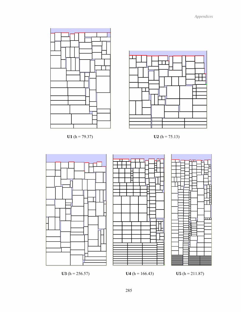
Appendices
U1 (h = 79.37) U2 (h = 75.13)
U3 (h = 256.57) U4 (h = 166.43) U5 (h = 211.87)
285

Appendices
APPENDIX B – Layouts for Irregular Benchmarks
B.1 – Solutions from Chapter Seven (Trigonometry Packing)
Albano: 10292.90 units (93.3s)
Blasz1: 27.20 units (501.9s) Blasz2: 25.28 units (10.9s)
286

Appendices
Dagli: 60.57 units (188.8s) Dighe1: 1292.30 units (8.8s) Dighe2: 1260.00 units (7.1s)
Fu: 32.80 units (20.7s Jakobs1: 11.86 units (43. Jakobs2: 25.80 units (81.4s) ) 4s)
287

Appendices
Mao: 1854.30 units (29.7s) Marques: 80.00 units (4.8s)
Poly1A: 14.00 units (12.5s) Poly2A: 28.17 units (120.6s) 0 3 units (1515.5s) Poly3A: 4 .3
Poly4A: 54.93 units (203.2s) Poly5A: 69.37 units (475.6s)
288

Appendices
Poly2B: 30.0 units (179.9s) Poly3B: 40.74 units (417.7s)
Poly4B: 51.73 un Poly5B: 60.54 units (676.6s) its (95.7s)
SHAPES0: 65.00 units (332.4s)
289

Appendices
APES1: 58.40 units (1810.1s) HAPES: 59.00 units (31.4s) SH S
: 63.00 units (806.5s) SWIM: 6462.40 units (607.4s)
SHIRTS
TROUSERS: 243.40 units (3612.0s)
290

Appendices
Profiles1: 1377.74 units Profiles2: 3216.10 units
Profiles3: 8193.89 units
Profiles4: 2453.12 units
291

Appendices
Profiles5: 3332.70 units rofiles6: 3097.86 units Profiles7: 1296.30 units P
Profiles8: 1318.70 units Profiles9: 1290.67 units
Profiles10: 11160.10 units
292
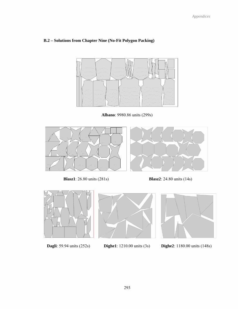
Appendices
B.2 – Solutions from Chapter Nine (No-Fit Polygon Packing)
Albano: 9980.86 units (299s)
Blasz1: 26.80 units (281s) Blasz2: 24.80 units (14s)
Dagli: 59.94 units (252s) Dighe1: 1210.00 units (3s) Dighe2: 1180.00 units (148s)
293

Appendices
Fu: 31.60 units (139s) Jakobs1: 11.50 units (29s) Jakobs2: 24.70 units (51s)
Mao: 1821.70 units (152s) Marques: 78.00 units (21s)
Poly1A: 13.30 units (254s) Poly2A: 27.09 units (239s) Poly3A: 40.45 units (429s)
294

Appendices
Poly4A: 54.60 units (224s) Poly5A: 68.84 units (300s)
Poly2B: 29.63 units (189s) Poly3B: 40.50 units (114s)
Poly4B: 51.18 units (176s) Poly5B: 60.86 units (299s)
295

Appendices
SHAPES0: 60.00 units (274s)
SHAPES1: 55.00 units (166s) SHAPES: 56.00 units (226s)
SHIRTS: 63.16 units (806s) SWIM: 6270.88 units (141s)
TROUSERS: 243.00 units (12484s)
296

Appendices
Profiles1: 1359.90 units Profiles2: 3194.19 units
Profiles3: 7881.13 units
Profiles4: 2425.26 units
297
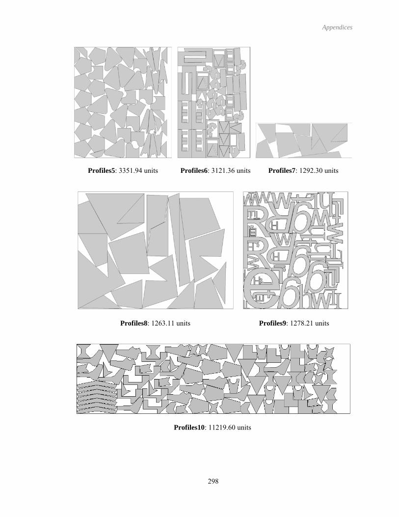
Appendices
Profiles5: 3351.94 units Profiles6: 3121.36 units Profiles7: 1292.30 units
Profiles8: 1263.11 units Profiles9: 1278.21 units
Profiles10: 11219.60 units
298
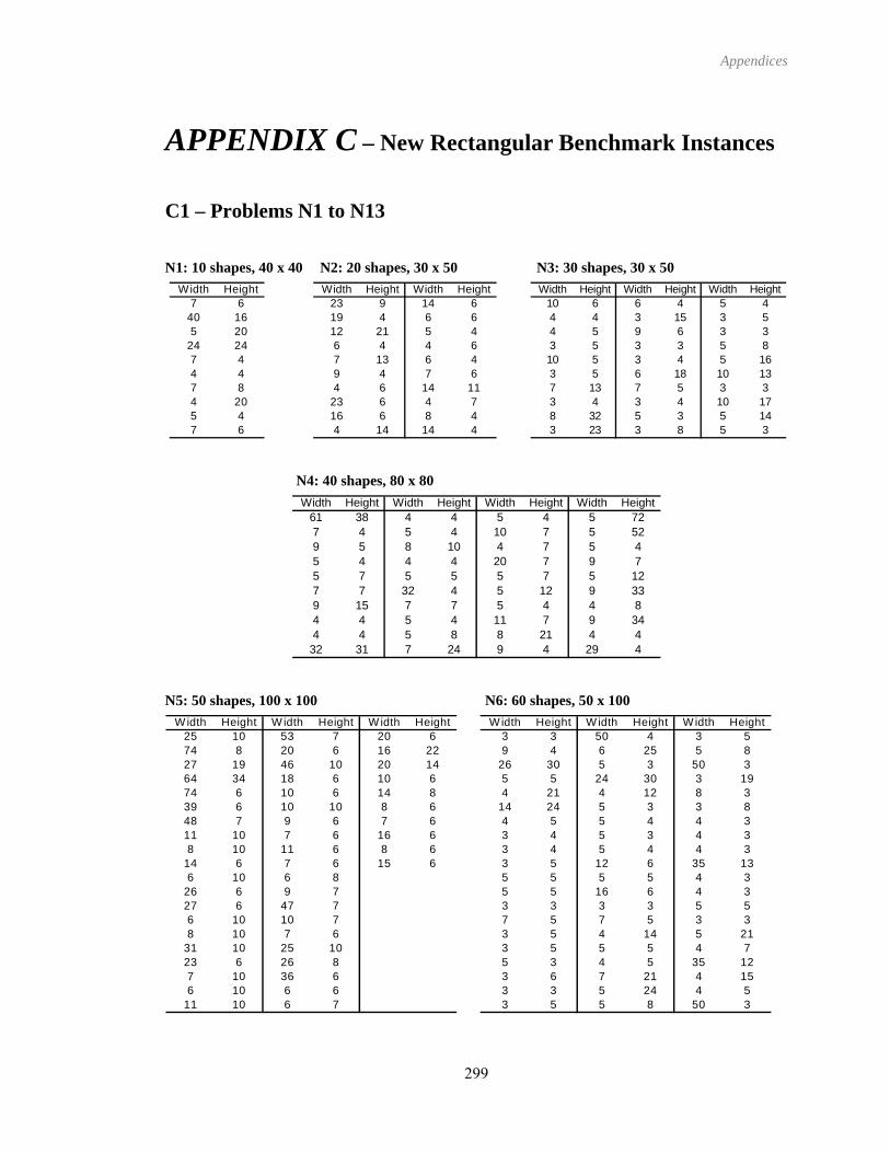
Appendices
APPENDIX C – New Rectangular Benchmark Instances
C1 – Problems N1 to N13
N1: 10 shapes, 40 x 40 N2: 20 shapes, 30 x 50 N3: 30 shapes, 30 x 50
Width Height7 6
40 165 20
24 247 44 47 84 205 47 6
Width Height Width Height23 9 14 619 4 6 612 21 5 46 4 4 67 13 6 49 4 7 64 6 14 11
23 6 4 716 6 8 44 14 14 4
Width Height Width Height Width Height10 6 6 4 5 44 4 3 15 3 54 5 9 6 3 33 5 3 3 5 810 5 3 4 5 163 5 6 18 10 137 13 7 5 3 33 4 3 4 10 178 32 5 3 5 143 23 3 8 5 3
N4: 40 shapes, 80 x 80
Width Height Width Height Width Height Width Height61 38 4 4 5 4 5 727 4 5 4 10 7 5 529 5 8 10 4 7 5 45 4 4 4 20 7 9 75 7 5 5 5 7 5 127 7 32 4 5 12 9 339 15 7 7 5 4 4 84 4 5 4 11 7 9 344 4 5 8 8 21 4 4
32 31 7 24 9 4 29 4 N5: 50 shapes, 100 x 100 N6: 60 shapes, 50 x 100
Width Height W idth Height W idth Height25 10 53 7 20 674 8 20 6 16 2227 19 46 10 20 1464 34 18 6 10 674 6 10 6 14 839 6 10 10 8 648 7 9 6 7 611 10 7 6 16 68 10 11 6 8 6
14 6 7 6 15 66 10 6 8
26 6 9 727 6 47 76 10 10 78 10 7 6
31 10 25 1023 6 26 87 10 36 66 10 6 6
11 10 6 7
Width Height W idth Height W idth Height3 3 50 4 3 59 4 6 25 5 8
26 30 5 3 50 35 5 24 30 3 194 21 4 12 8 3
14 24 5 3 3 84 5 5 4 4 33 4 5 3 4 33 4 5 4 4 33 5 12 6 35 135 5 5 5 4 35 5 16 6 4 33 3 3 3 5 57 5 7 5 3 33 5 4 14 5 213 5 5 5 4 75 3 4 5 35 123 6 7 21 4 153 3 5 24 4 53 5 5 8 50 3
299

Appendices
N7: 70 shapes, 80 x 100 N8: 80 shapes, 100 x 80
Width Height W idth Height W idth Height6 82 3 6 4 23 2 2 2 12 73 38 37 22 2 4
19 23 24 2 3 27 36 13 2 3 52
46 12 11 2 3 143 4 4 33 3 23 2 9 12 18 42 82 5 2 19 593 15 25 5 23 23 2 2 23 22 2 22 2 3 23 37 2 22 2 3 42 2 3 223 2 9 223 40 3 56 2 3 407 2 3 47 7 8 22 2 3 20
18 2 2 213 7 2 22 4 3 42 2 2 28 2 3 23 2 23 38
28 22 2 222 2 11 38
Width Height W idth Height W idth Height17 6 3 15 12 103 5 12 6 18 4
16 5 37 15 3 54 4 3 4 5 164 3 3 3 20 54 5 34 11 4 54 4 4 5 4 5
12 4 23 4 8 63 11 23 4 10 33 4 37 3 3 4
40 13 7 50 3 78 20 20 3 11 193 9 3 5 13 434 28 4 7 5 209 11 10 6 5 113 22 7 6 4 44 3 5 8 9 34 3 3 3 3 4
20 4 4 4 3 144 35 9 24 10 6
N9: 100 shapes, 50 x 150
W H W H W H W H W H W5 3 3 5 4 3 3 4 3 3 33 5 4 3 5 3 12 23 3 5 45 3 47 7 4 4 28 7 3 3 65 5 4 4 4 3 4 3 9 5 74 5 11 3 8 7 3 40 3 3 34 15 3 4 3 3 4 5 5 3 45 5 4 5 4 4 24 4 3 20 33 3 19 6 28 5 4 3 3 3 47
44 35 3 5 9 5 3 3 3 4 3
N10: 200 shapes, 70 x 150
W H W H W H W H W H W2 3 2 2 2 2 6 2 2 2 23 3 2 2 3 2 3 2 2 2 23 21 2 3 3 2 2 2 2 8 13
54 33 3 3 25 3 25 3 20 2 28 5 3 2 2 2 2 8 2 3 22 2 2 2 2 2 2 2 4 2 23 2 3 62 2 2 2 2 2 3 22 2 3 5 2 4 2 3 3 8 23 2 2 2 60 25 3 3 2 11 25 3 2 3 2 2 5 13 2 3 192 2 2 2 59 18 4 3 5 12 9
29 3 6 6 5 28 4 2 32 2 173 3 3 3 3 2 2 2 2 2 52 3 2 2 12 3 2 2 3 2 26 50 2 2 29 2 48 3 5 2 23 2 2 2 2 2 2 2 2 3 5
22 6 7 2 3 6 3 3 3 3 23
4 423 344 293 12
11 84 217 35
23 353 44 5
H W H W H6 4 28 5 35 3 5 4 35 3 3 28 113 4 4 3 38 4 4 4 35 3 35 10 35 3 13 10 54 4 3 3 83 3 3 3 4
H W H W H2 4 6 2 22 51 3 2 32 3 2 6 32 9 2 34 23 5 9 2 22 2 2 13 333 25 2 2 22 2 2 16 33 3 2 4 28 3 3 2 74 2 3 2 58 32 2 2 22 11 3 2 22 17 6 2 23 3 2 7 23 2 2 8 32 2 2 2 2
300
11 84 33 58 107 33 33 5
16 57 43 10
W H W H W H W H4 32 3 4 3 10 3 143 5 3 39 4 98 3 19 17 15 503 5 10 5 12 273 4 6 54 22 44 3 9 4 8 44 9 7 3 3 45 3 3 54 16 54 5 3 5 18 4
W H W H W H W H3 12 3 2 5 2 6 22 2 14 3 3 3 8 3
16 31 2 2 4 4 2 22 2 3 12 42 3 2 23 2 2 2 2 2 3 3
13 3 4 2 3 11 2 32 2 3 3 2 3 2 32 6 2 3 2 2 2 3
16 4 27 2 2 2 2 28 3 3 2 31 28 19 22 5 2 4 2 2 2 23 2 7 5 2 3 2 23 3 5 2 2 2 20 22 2 3 10 2 22 2 5 3 2 72 2 14 3 2 22 3 18 3 5 6

Appendices
N11: 300 shapes, 70 x 150
W H W H W H W H W H W H W H W H W H W H W H W H3 3 3 4 3 20 3 2 3 17 70 7 2 2 3 3 2 3 2 2 2 6 32 10
17 3 3 2 2 5 19 23 3 2 2 3 2 2 6 9 2 3 3 3 3 3 3 321 9 2 3 3 3 3 2 2 2 32 6 9 11 3 2 3 3 8 4 11 4 2 22 3 2 5 2 2 3 2 63 3 4 2 4 16 2 13 2 2 9 3 5 5 2 32 11 2 10 3 2 2 2 2 2 4 2 3 3 3 2 6 17 9 2 9 5 2 22 3 2 3 7 3 2 3 2 2 2 7 3 3 2 2 3 5 8 2 4 6 3 123 3 3 2 2 3 19 19 4 3 2 3 2 3 2 3 3 2 6 2 13 17 3 9
31 17 2 3 10 11 3 2 3 2 2 2 2 2 15 2 2 2 2 4 2 2 2 52 2 3 2 5 4 2 5 8 2 15 17 7 2 2 2 4 2 2 3 2 14 14 172 3 3 3 3 2 2 3 4 3 3 2 2 6 2 3 3 2 8 3 14 17 12 2
20 3 2 5 3 2 3 3 3 10 2 3 23 6 2 2 2 7 10 2 3 3 2 22 3 2 3 38 3 2 3 3 2 2 2 18 2 2 2 10 4 3 6 3 8 11 42 3 2 2 48 2 3 2 3 2 3 3 3 2 3 4 3 2 30 5 27 2 3 4
70 4 12 14 2 5 3 3 2 2 3 2 4 8 3 3 2 2 3 2 10 21 3 35 4 2 3 6 2 4 11 2 2 30 4 3 2 24 2 2 3 10 3 2 4 7 3
23 2 3 30 3 3 2 3 2 2 21 3 10 2 4 13 4 3 3 4 6 2 2 35 3 3 3 8 16 2 3 3 3 3 3 8 3 3 16 2 3 2 2 21 2 3 22 12 2 3 2 3 3 3 2 23 2 2 10 2 26 6 3 2 3 2 4 2 4 32 3 2 3 2 3 2 3 2 3 2 3 2 8 2 2 3 3 5 2 2 4 3 22 3 8 3 3 2 3 5 2 3 3 3 5 2 3 2 3 3 7 3 7 3 16 27 2 4 2 15 2 2 2 18 2 3 5 3 5 2 3 6 16 3 4 2 3 5 52 3 2 3 15 6 2 3 2 3 3 3 3 2 5 11 2 2 2 2 3 2 4 115 16 2 2 2 3 2 2 3 2 3 3 2 2 70 5 2 2 3 3 3 2 5 172 2 24 7 2 3 4 6 2 3 27 4 5 4 3 5 25 2 12 4 19 5 3 4
15 6 3 3 3 3 5 3 3 3 3 3 5 16 2 2 2 2 2 2 10 4 2 4
N12: 500 shapes, 100 x 300
W H W H W H W H W H W H W H W H W H W H W H W H5 4 4 3 5 3 3 5 3 4 9 3 4 4 2 8 3 7 5 3 4 7 5 3 7 5 33 1 3 1 2 3 3 5 2 0 5 5 3 1 2 3 3 3 4 4 3 3 4 8 6 1 0 1 2 5 4 4
4 9 3 3 5 3 2 6 3 3 3 3 3 3 3 4 3 4 3 5 2 2 5 3 5 6 9 83 5 3 3 5 3 4 4 3 3 4 3 5 4 3 2 9 3 1 0 4 6 4 5 3 35 5 4 4 1 7 3 3 3 3 3 5 1 6 5 5 3 3 3 4 9 2 3 5 6 9 53 5 3 5 5 7 3 3 3 3 3 3 6 3 4 3 5 3 4 3 7 5 9 4 3 35 5 5 5 5 9 3 3 5 1 0 4 5 3 4 4 7 3 4 1 2 3 1 6 8 3 33 3 5 4 3 7 3 1 6 3 3 5 4 3 3 1 2 3 3 3 3 1 3 4 3 3 44 1 0 7 3 5 4 1 3 3 5 3 3 3 2 1 3 3 3 3 8 4 1 5 8 4 4 1 0 2 73 4 5 3 1 0 1 0 1 2 3 3 3 3 3 4 3 8 5 8 3 4 4 3 3 3 3 2 14 1 1 5 4 1 4 3 3 5 3 5 4 3 3 3 1 4 5 3 6 8 3 9 5 1 8 1 0 1 73 7 5 3 3 4 3 3 3 1 3 3 4 3 3 5 4 7 1 5 3 1 2 4 5 3 39 8 3 4 3 3 3 4 3 3 5 3 3 3 4 5 5 4 3 3 5 5 3 97 3 3 3 4 3 5 5 3 3 3 3 4 3 3 3 4 3 3 3 6 2 7 3 3 3 5 15 5 3 5 3 3 4 4 4 5 3 3 5 3 5 4 5 2 0 3 8 3 1 0 8 9 85 3 3 3 3 3 5 3 4 5 3 5 3 6 3 4 6 5 5 5 1 4 3 6 74 5 3 4 3 3 5 4 3 3 3 4 3 3 4 7 3 3 3 3 5 3 3 3 3 35 4 7 3 3 3 5 5 5 4 1 9 4 1 0 3 1 2 3 4 3 4 3 4 3 2 5 7 2 05 3 5 8 3 3 3 1 8 5 3 2 1 3 3 3 3 5 4 3 5 8 4 3 3 83 5 3 4 1 2 5 6 3 3 1 2 3 3 3 2 2 1 0 6 1 6 3 5 3 3 4 9 4 3
1 2 5 5 5 5 3 3 6 5 1 0 4 5 4 6 3 5 4 1 0 3 1 0 3 3 4 1 33 3 3 6 5 5 3 3 3 3 3 4 2 0 4 3 5 9 3 5 3 3 6 3 43 4 3 3 3 4 3 4 1 5 2 3 3 7 4 5 5 5 5 1 1 4 1 6 3 3 6 3 53 3 3 3 5 3 3 3 3 3 7 4 3 3 3 5 4 3 3 4 1 8 2 4 3 53 5 5 3 4 4 3 3 5 5 3 1 1 3 3 3 4 5 5 4 3 3 9 3 3 45 3 3 5 3 3 4 3 3 3 3 3 4 4 3 5 3 3 4 5 4 5 3 63 5 3 3 3 4 3 3 3 4 3 3 3 7 3 4 5 3 3 3 5 7 3 43 7 5 3 1 4 2 7 7 6 1 9 1 2 4 3 3 3 3 5 3 4 3 3 4 1 1 4 35 5 3 3 3 3 4 3 4 3 3 5 3 3 3 5 4 1 4 1 8 3 9 3 2 4 45 3 3 4 3 4 3 3 5 1 8 8 7 3 4 4 3 1 8 2 5 5 4 3 1 2 3 65 3 3 5 1 1 3 1 2 1 9 3 3 3 3 1 2 4 3 4 4 3 3 2 1 3 6 3 3 4 33 7 5 3 3 3 3 1 7 3 4 4 2 4 5 4 3 5 3 4 3 2 3 3 4 5 65 3 3 2 1 4 4 3 3 3 3 1 8 5 3 3 8 3 1 2 1 0 2 5 3 3 1 6 8 3 0 43 3 4 4 3 3 3 3 3 4 3 3 5 5 3 4 1 1 4 9 5 1 3 3 6 3 33 4 3 2 8 3 4 3 5 3 7 4 4 3 4 4 5 5 3 3 5 2 3 3 4 1 7 35 4 3 3 3 3 3 5 3 1 0 3 5 1 8 5 3 3 5 4 4 3 1 1 3 5 4 54 4 3 1 4 4 5 3 3 4 3 4 3 3 5 3 3 5 3 3 3 4 2 6 5 53 4 3 1 5 4 5 4 3 4 5 1 8 2 5 3 3 5 3 1 5 4 3 1 6 1 4 3 3 63 3 3 3 3 5 4 3 5 1 1 3 3 4 3 2 8 5 3 3 3 3 4 1 04 8 4 4 1 8 9 3 3 4 4 3 3 4 6 4 5 8 3 3 3 3 45 4 3 5 4 1 6 4 3 3 3 3 3 9 5 3 3 4 5 4 5 4 0 1 05 3 5 3 3 4 3 4 3 1 0 3 4 3 5 3 5 6 1 2 3 1 1 9 1 8
301

Appendices
N13: 3152 shapes, 640 x 960
Obtained by a 4 x 4 extension of problem c7p2 (197 shapes) from (Hopper and Turton, 2001) [110].
C7P2C7P2 C7P2 C7P2
C7P2C7P2 C7P2 C7P2
C7P2C7P2 C7P2 C7P2
C7P2C7P2 C7P2 C7P2
640
960
240
160
302

Appendices
C2 – Problems MT1 to MT10
MT1 – Rectangles = 100, Sheet = 400 x 600 MT2 – Rectangles = 150, Sheet = 300 x 900
Width Height Quantity49.5 49.5 10
20.5 22.8 7
10
12.5 24.1 845.9 80.1 1032.8 45.2 1215.7 10.2 835.2 29.777 1030.5 176.8 57.5 105.8 3
31.4 10.8 970.4 93.410 30 8
Width Height Quantity
15
44.7 60 1531 20.3 15
50.6 5 1510 20 1530 58.8 15
60.5 50 1544.2 85 1532.3 3021 50.2 15
30.5 29 15
0
MT3 – Rectangles = 200, Sheet = 400 x 900 MT4 – Rectangles = 300, Sheet = 600 x 130
Width Height Quantity
12
8
7
42.5 65.5 1090.3 80.3 952.5 24.1 1645.9 80.1 1032.8 15.2 1515.7 10.2 831.2 9.777 1060.5 36.8 770.5 55.820.5 22.8 711.4 40.8 1550.4 56.4 1014 28
30.3 125.1 28.3 12.4 14
14.1 20.1 45.9 6.1 12
130.4 114.8 113.2 8.13.4 20.3 6
40.3 10.2 540.2 30.6 534.8 22.5 7
Width Height Quantity5
9
24
2
20
20 7043 71 1080 20 825 26 20
101 76 530 13 19
170 2010 15 2037 13 1599 55 12
111 52 440 50 1050 60 1010 15 2095 37 1767 8743 82 1034 57 2010 169 515 9018 18 520 15 1032 39 2062 80
303

Appendices
MT5 – Rectangles = 500, Sheet = 800 x 1400 MT6 – Rectangles = 100, Sheet = 400 x 500
Width Height Quantity20 70 543 71 1080 20 825 26 20
101 76 530 13 19
170 20 910 15 2037 13 1599 55 12
111 52 440 50 1050 60 1010 15 2095 37 1767 87 2443 82 1034 57 2010 169 515 90 218 18 520 15 1032 39 2062 80 20
Width Height Quant10916
80.1 10158
31.2 9.777 10
2
50
14 28 8
2130.4 114.8 1
76557
ity42.5 65.590.3 80.352.545.9
24.1
32.8 15.215.7 10.2
60.5 36.817
70.5 55.820.5 22.8 711.4 40.8 150.4 56.4 1
30.3 125.1 28.3 12.4 14
14.1 20.1 45.9 6.1 1
13.2 8.13.4 20.3
40.3 10.240.2 30.634.8 22.5
Width Height Width Height27.512 234.999 39.306 31.992199.36 33.779 31.982 39.161196.456 35.04 39.306 31.492180.646 41.972 44.37 26.295177.68 42.868 28.545 41.972170.417 37.106 44.37 25.49433.478 172.228 35.51 33.77939.306 159.304 26.956 41.97231.982 157.449 44.531 23.544106.471 81.204 42.603 25.45125.378 160.305 33.328 33.779158.302 19.435 33.153 33.77941.07 135.208 39.306 27.559
139.246 33.795 42.496 23.544137.903 25.451 22.971 42.868115.684 44.195 42.209 23.54432.775 126.51 21.769 42.86844.37 109.042 19.971 44.195
106.471 45.306 41.07 22.68538.817 23.544111.667 36.305
17.658 125.495 36.809 25.451104.507 23.544 38.595 23.54447.236 41.972 24.477 37.10644.44 44.195 24.354 37.10640.17 44.195 26.753 33.77947.525 36.305 23.07 37.10644.37 38.539 16.851 42.86839.421 42.868 23.09 36.30538.791 42.868 16.251 42.86841.07 40.182 17.063 41.97244.37 36.489 16.514 41.97242.835 37.106 15.596 41.972
MT7 – Rectangles = 150, Sheet = 400 x 500 Width Height Width Height Width Height Width Height Width Height Width Height202.076 33.656 37.913 12.586 27.544 35.951 16.711 33.656 7.302 25.987 14.725 21.89117.307 199.243 37.913 24.104 17.425 35.951
.339 10.01 21.8911
5612.162 14.279 35.951
19.55 33.656 25.208 25.987 8.172 21.89126.547 197.95 37.913 30.366 13.814 35.951 16.388 33.656 25.922 21197.837 21.891 37.913 35.627 30.359 35.951 33.566 21.891 25.754 10.646 16.5 21.89193.599 21.756 37.913 12.889 31.091 35.951 32.804 25.578 24.034 25.578 17.517 21.89116.023 193.293 37.913 17.879 33.608 35.951 32.592 19.854 14.79 25.578 11.937 21.7
32.508 25.987 19.477 25.578 20.915 21.756190.63 28.737 37.913190.63 177.112 37.913 18.428 35.444 35.951 8.393 31.436 6.61 25.578 14.659 21.75623.793 187.358 37.913 27.532 35.851 31.436 18.788 31.436 18.738 25.578 6.919 21.339
.177 17.307 21.275186.312 25.177 37.908 10.646 35.427 10.266 6.096 31.436 19.083 25185.174 19.854 37.473 19.854 34.974 21.339 15.889 31.436 23.094 25.177 20.212 10.646184.718 10.614 37.154 11.027 34.839 25.578 54
29 25.177 18.025 19.8547
7 054681
.671 16.176 10.348
31.162 25.987 21.316 25.177 8.307 19.834.457 184.483 37.154 28.582 23.793 34.60 30.954 21.339 20.426 25.177 12.866 19.854183.673 25.987 37.154 11.165 34.457 24.59 30.29 25.578 21.269181.449 25.578 37.154 22.976 34.457 17.64 17.307 27.967 24.503 10.646 8.683 19.85416.176 180.713 37.154 6.785 16.176 34.04 27.336 25.987 24.228 19.854 11.245 19.854178.305 10.646 37.154 6.75 33.905 25.17
11.989 22.309 33.65626.547 26.855 23.793 22.539 16.176 18.2
37.913 177.419 37.154 26.547 6.365 23.793 14.862 16.588 10.6176.29 35.951 37.154 10.495 6.897 33.656 26.547 17.964 23.793 10.598 16.176 9.6174.217 21.339 36.969 25.578 21.813 33.656 26.547 14.298 23.793 17173.4 31.436 16.176 36.758 14.269 33.656 26.547 18.662 23.793 13.63 16.023 12.556
171.226 10.266 36.555 25.177 8.266 33.656 26.547 23.889 23.494 19.854 13.898 10.64637.154 170.152 16.176 36.494 31.774 33.656 26.547 17.168 16.176 22.899 13.719 10.61438.572 10.646 36.316 10.646 18.591 33.656 15.029 25.987 22.585 21.339 7.944 10.64638.04 25.177 20.146 35.951 21.356 33.656 23.693 25.987 21.037 21.891 8.216 10.614
304
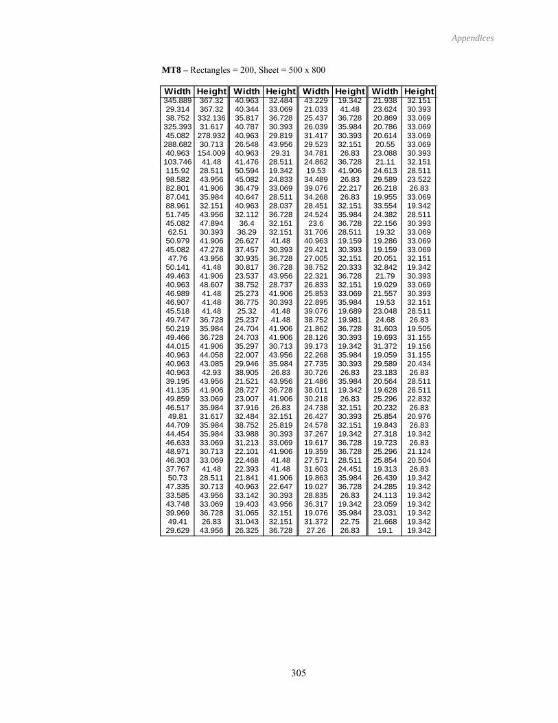
Appendices
MT8 – Rectangles = 200, Sheet = 500 x 800
Width Height Width Height Width Height Width Height345.889 367.32 40.963 32.484 43.229 19.342 21.938 32.15129.314 367.32 40.344 33.069 21.033 41.48 23.624 30.39338.752 332.136 35.817 36.728 25.437 36.728 20.869 33.069325.393 31.617 40.787 30.393 26.039 35.984 20.786 33.06945.082 278.932 40.963 29.819 31.417 30.393 20.614 33.069288.682 30.713 26.548 43.956
129.523 32.151 20.55 33.069
40.963 154.009 40.963 29.3 34.781 26.83 23.088 30.393103.746 41.48 41.476 28.511 24.862 36.728 21.11 32.151115.92 28.511 50.594 19.342 19.53 41.906 24.613 28.51198.582 43.956 45.082 24.833 34.489 26.83 29.589 23.52282.801 41.906 36.479 33.069 39.076 22.217 26.218 26.8387.041 35.984 40.647 28.511
37.728
34.268 26.83 19.955 33.06988.961 32.151 40.963 28.0 28.451 32.151 33.554 19.34251.745 43.956 32.112 3645.
24.524 35.984 24.382 28.511082 47.894 36.4 32.151 23.6 36.728 22.156 30.393
62.51 30.393 36.29 32.151 31.706 28.511 19.32 33.06950.979 41.906 26.627 41.48 40.963 19.159 19.286 33.06945.082 47.278 37.457 30.393 29.421 30.393 19.159 33.06947.76 43.956 30.935 36.728 27.005 32.151 20.051 32.15150.141 41.48 30.817 36.728 38.752 20.333 32.842 19.34249.463 41.906 23.537 43.956 22.321 36.728 21.79 30.39340.963 48.607 38.752 28.737 26.833 32.151 19.029 33.06946.989 41.48 25.273 41.906 25.853 33.069 21.557 30.39346.907 41.48 36.775 30.393 22.895 35.984 19.53 32.15145.518 41.48 25.32 41.48 39.076 19.689 23.048 28.51149.747 36.728 25.237 41.48 38.752 19.981 24.68 26.8350.219 35.984 24.704 41.906 21.862 36.728 31.603 19.50549.466 36.728 24.703 41.906 28.126 30.393 19.693 31.15544.015 41.906 35.297 30.713 39.173 19.342 31.372 19.15640.963 44.058 22.007 43.956 22.268 35.984 19.059 31.15540.963 43.085 29.946 35.984 27.735 30.393 29.589 20.43440.963 42.93 38.905 26.83 30.726 26.83 23.183 26.8339.195 43.956 21.521 43.956 21.486 35.984 20.564 28.51141.135 41.906 28.727 36.728 38.011 19.342 19.628 28.51149.859 33.069 23.007 41.906 30.218 26.83 25.296 22.83246.517 35.984 37.916 26.83
519
24.738 32.151 20.232 26.8349.81 31.617 32.484 32.1 26.427 30.393 25.854 20.97644.709 35.984 38.752 25.81 24.578 32.151 19.843 26.8344.454 35.984 33.988 30.393 37.267 19.342 27.318 19.34246.633 33.069 31.213 33.069 19.617 36.728 19.723 26.8348.971 30.713 22.101 41.906 19.359 36.728 25.296 21.12446.303 33.069 22.468 41.48 27.571 28.511 25.854 20.50437.767 41.48 22.393 41.48 31.603 24.451 19.313 26.8350.73 28.511 21.841 41.906 19.863 35.984 26.439 19.34247.335 30.713 40.963 22.647 19.027 36.728 24.285 19.34233.585 43.956 33.142 30.393 28.835 26.83 24.113 19.34243.748 33.069 19.403 43.956 36.317 19.342 23.059 19.34239.969 36.728 31.065 32.151 19.076 35.984 23.031 19.34249.41 26.83 31.043 32.151 31.372 22.75 21.668 19.34229.629 43.956 26.325 36.728 27.26 26.83 19.1 19.342
305
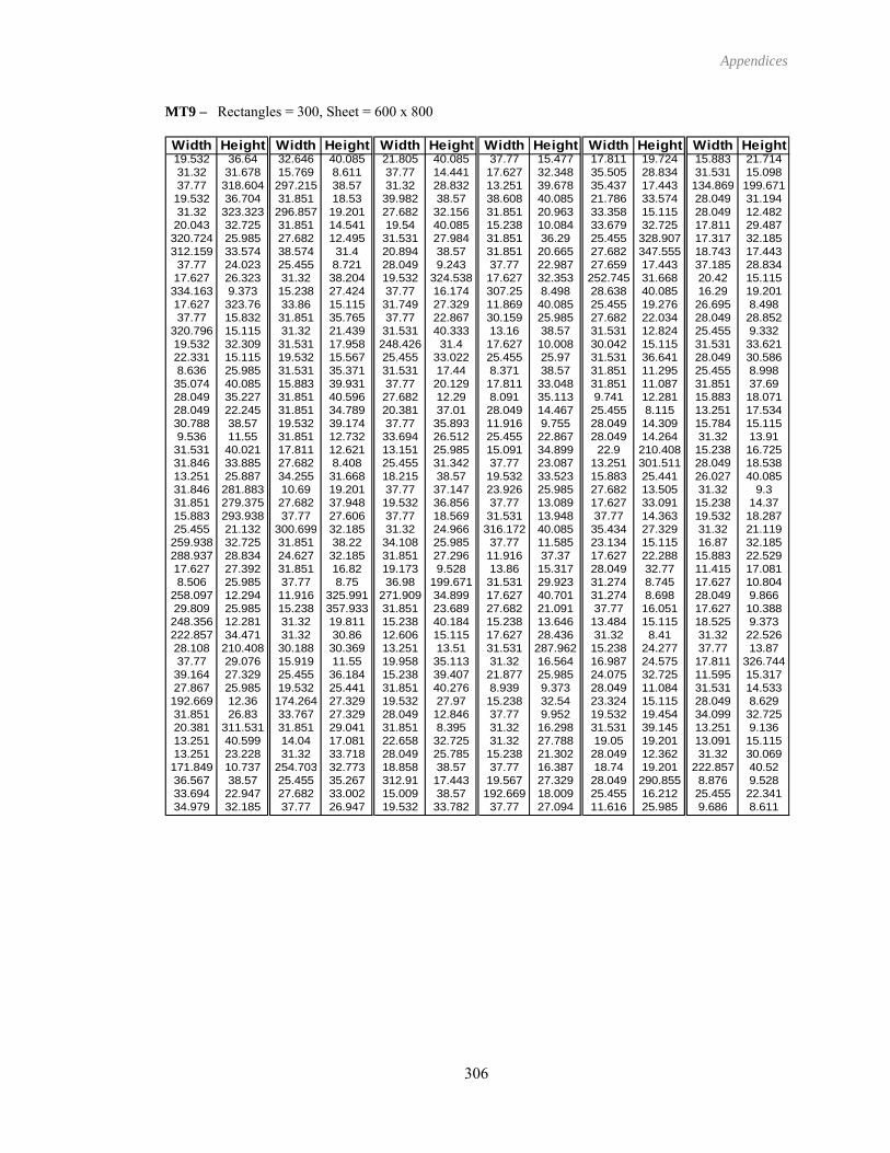
Appendices
MT9 – Rectangles = 300, Sheet = 600 x 800 Width Height Width Height Width Height htWidth Height Width Height Width Heig19.532 36.64 32.646 40.085 21.805 40.085 37.77 15.477 17.811 19.724 15.883 21.71431.32 31.678 15.769 8.611 37.77 14.441 17.627 32.348 35.505 28.834 31.531 15.09837.77 318.604 297.215 38.57 31.32 28.832 13.251 39.678 35.437 17.443 134.869 199.67119.532 36.704 31.851 18.53 39.982 38.57 38.608 40.085 21.786 33.574 28.049 31.19431.32 323.323 296.857 19.201 27.682 32.156 31.851 20.963 33.358 15.115 28.049 12.48220.043 32.725 31.851 14.541 19.54 40.085 15.238 10.084 33.679 32.725 17.811 29.487320.724 25.985 27.682 12.495 31.531 27.984 31.851 36.29 25.455 328.907 17.317 32.185312.159 33.574 38.574 31.4 20.894 38.57 31.851 20.665 27.682 347.555 18.743 17.44337.77 24.023 25.455 8.721 28.049 9.243 37.77 22.987 27.659 17.443 37.185 28.83417.627 26.323 31.32 38.204 19.532 324.538 17.627 32.353 252.745 31.668 20.42 15.115334.163 9.373 15.238 27.424 37.77 16.174 307.25 8.498 28.638 40.085 16.29 19.20117.627 323.76 33.86 15.115 31.749 27.329 11.869 40.085 25.455 19.276 26.695 8.49837.77 15.832 31.851 35.765 37.77 22.867 30.159 25.985 27.682 22.034 28.049 28.852
320.796 15.115 31.32 21.439 31.531 40.333 13.16 38.57 31.531 12.824 25.455 9.33219.532 32.309 31.531 17.958 248.426 31.4 17.627 10.008 30.042 15.115 31.531 33.62122.331 15.115 19.532 15.567 25.455 33.022 25.455 25.97 31.531 36.641 28.049 30.5868.636 25.985 31.531 35.371 31.531 17.44 8.371 38.57 31.851 11.295 25.455 8.99835.074 40.085 15.883 39.931 37.77 20.129 17.811 33.048 31.851 11.087 31.851 37.6928.049 35.227 31.851 40.596 27.682 12.29 8.091 35.113 9.741 12.281 15.883 18.07128.049 22.245 31.851 34.789 20.381 37.01 28.049 14.467 25.455 8.115 13.251 17.53430.788 38.57 19.532 39.174 37.77 35.893 11.916 9.755 28.049 14.309 15.784 15.1159.536 11.55 31.851 12.732 33.694 26.512 25.455 22.867 28.049 14.264 31.32 13.9131.531 40.021 17.811 12.621 13.151 25.985 15.091 34.899 22.9 210.408 15.238 16.72531.846 33.885 27.682 8.408 25.455 31.342 37.77 23.087 13.251 301.511 28.049 18.53813.251 25.887 34.255 31.668 18.215 38.57 19.532 33.523 15.883 25.441 26.027 40.08531.846 281.883 10.69 19.201 37.77 37.147 23.926 25.985 27.682 13.505 31.32 9.331.851 279.375 27.682 37.948 19.532 36.856 37.77 13.089 17.627 33.091 15.238 14.3715.883 293.938 37.77 27.606 37.77 18.569 31.531 13.948 37.77 14.363 19.532 18.28725.455 21.132 300.699 32.185 31.32 24.966 316.172 40.085 35.434 27.329 31.32 21.119259.938 32.725 31.851 38.22 34.108 25.985 37.77 11.585 23.134 15.115 16.87 32.185288.937 28.834 24.627 32.185 31.851 27.296 11.916 37.37 17.627 22.288 15.883 22.52917.627 27.392 31.851 16.82 19.173 9.528 13.86 15.317 28.049 32.77 11.415 17.0818.506 25.985 37.77 8.75 36.98 199.671 31.531 29.923 31.274 8.745 17.627 10.804
258.097 12.294 11.916 325.991 271.909 34.899 17.627 40.701 31.274 8.698 28.049 9.86629.809 25.985 15.238 357.933 31.851 23.689 27.682 21.091 37.77 16.051 17.627 10.388248.356 12.281 31.32 19.811 15.238 40.184 15.238 13.646 13.484 15.115 18.525 9.373222.857 34.471 31.32 30.86 12.606 15.115 17.627 28.436 31.32 8.41 31.32 22.52628.108 210.408 30.188 30.369 13.251 13.51 31.531 287.962 15.238 24.277 37.77 13.8737.77 29.076 15.919 11.55 19.958 35.113 31.32 16.564 16.987 24.575 17.811 326.74439.164 27.329 25.455 36.184 15.238 39.407 21.877 25.985 24.075 32.725 11.595 15.31727.867 25.985 19.532 25.441 31.851 40.276 8.939 9.373 28.049 11.084 31.531 14.533192.669 12.36 174.264 27.329 19.532 27.97 15.238 32.54 23.324 15.115 28.049 8.62931.851 26.83 33.767 27.329 28.049 12.846 37.77 9.952 19.532 19.454 34.099 32.72520.381 311.531 31.851 29.041 31.851 8.395 31.32 16.298 31.531 39.145 13.251 9.13613.251 40.599 14.04 17.081 22.658 32.725 31.32 27.788 19.05 19.201 13.091 15.11513.251 23.228 31.32 33.718 28.049 25.785 15.238 21.302 28.049 12.362 31.32 30.069171.849 10.737 254.703 32.773 18.858 38.57 37.77 16.387 18.74 19.201 222.857 40.5236.567 38.57 25.455 35.267 312.91 17.443 19.567 27.329 28.049 290.855 8.876 9.52833.694 22.947 27.682 33.002 15.009 38.57 192.669 18.009 25.455 16.212 25.455 22.34134.979 32.185 37.77 26.947 19.532 33.782 37.77 27.094 11.616 25.985 9.686 8.611
306

Appendices
MT10 – Rectangles = 500, Sheet = 700 x 800 Width Height Width Height Width Height Width Height Width Height Width Height Width Height Width Height
6 .3647 69 .552
.3516 21.7113 .125 21.373 25.85 20.3511 .9431 87 15 39 .346
44.592 31.399 42.488 19.979 9 28.9162.4 34.171 42.488 19.232
30.27523
29.44 20.122 25.641 19.4224.701
.3515525
485
71.522
19.80330.602 40.017 35.661
799
43.359.831.055.351.56
41.694 31.723 18.759 34.171 .19.553
.44 24.412 25.267 36.84621.711
.1691
.12917.774
28.25 29.44 423.136.048
27.86 44.465 42.488 37.355 34.345 38.548 29.44 36.799 933.083 3
33.096 25.521 40.017 33.215 141.13 5
27 578 33.029
482 29.44 18.536 34.878 28.525029 .904892 .97331 36.189
.341 17.202 20.341 19.173 20.341 26.999 18.454 18.15223.44
8993
206
19.499 19.803 45.522 43.102 44.592 19.211 41.627 28.91 17.156 48.523 19.813 35.089 22.675 35.089 29.44 1724.349 369.233 40.017 42.207 32.06 28.129 40.017 30.49 20.341 45.337 32.784 37.653 25.267 36.77 27.398 19.3440.193 38.178 46.281 42.141 43.241 34.171 24.367 28.12 40.017 35.95 68.631 191.739 31.125 23.263 27.007 1934.878 314.222 40.017 16.742 29.44 47.905 31.125 271.041 21.483 44.033 47.729 25.521 34.878 18.066 26.163
35.815 18.389 24.50120
40.017 16.016 17.267 42.141 40.017 37.304 40.017 38.60 26.697 38.729 25.267 26.923144.76 44.427 41.694 25.318 34.878 42.189 144.76 27.94 23.044 42.141 40.55 18.389 3129.292 176.546 40.017 47.512 29.973 47.059 39.097 36.98 17.935 47.245 22.372 37.426 34.878 21.623 47.134 22
20.29298.58 25.521 44.592 42.746 40.017 21.77 28.021 42.14 21.98 43.102 29.255 40.856 25.878 27.652 42.413285.122 37.426 43.986 43.327 32.88 43.327 25.878 40.96 31.125 33.88 32.836 26.803 34.878 19.977 250.273 20.3547.134 269.997 29.44 25.1 45.373 43.102 126.825 47.24 273.429 34.171 44.592 18.385 34.878 18.311 20.161 25.58270.36 39.989 48.034 38.729 22.308 38.306 20.309 33.02 22.723 34.171 40.017 19.32 34.878 18.102 22.14
25.878 27.897 26.181 33.029 244.818 43.996 276.136 19
25.878 38.901 29.44 45.64942.488 22.494 29.44 46.162 20.341 45.321 42.488 27.202 34.878 24.905 25.878 33.323 444.592 28.418 36.62 38.548 29.44 46.424 40.017 44.475 42.413 30.264 19.187 39.989 19.828 33.029 40.01738.913 38.729 30.169 18.664 42.488 33.346 20.341 32.264 20.448 25.521 25.878 33.228 16.118 20.351 23.388 43.10
24.8019.203 46.777 44.592 19.219 45.482 41.13 31.125 37.911 68.631 28.516 19.147 25.521 40.017 44.542 20.34122.873 27.258 42.488 42.806 42.488 27.456 20.341 41.708 144.76 27.084 41.694 38.73420.341 282.291 144.76 18.681 26.316 41.13 37.956 28.916 24.309 42.141 48.278 25.189 18.767 38.729 20.34138.477 20.351 37.166 19.346 42.488 30.716 25.878 43.002 20.341 47.991 31.125 27.743 19.248 43.102 24.656 20272.463 28.129 46.238 38.729 31.748 44.033 42.488 25.954 44.081 19.346 29.973 44.369 31.125 21.287 19.978 22.6523.781 20.351 40.017 44.788 25.878 46.776 26.065 28.916 41.694 21.723 44.592 43.125 19.303 33.029 36.043 44.4623.249 34.171 42.413 42.381 20.653 34.171 44.592 23.772 34.878 47.284 16.194 19.346 31.125 42.709 42.488 30.5225.878 270.435 28.143 20.351 43.277 43.102 20.341 25.479 47.22 38.178 37.826 41.13 29.44 22.669 21.716 22.65275.81 18.389 26.973 25.583 42.488 44.159 31.125 47.517 20.341 42.549 41.694 16.852 25.878 25.803 260.276 38.5268.605 25.189 22.937 33.029 29.44 45.556 25.878 42.442 25.878 36.933 20.18 38.306 23.436 24.831 29.44 38.
4.112
259.574 30.463 41.694 40.813 16.846 43.102 29.44 38.808 32.888 25.189 44.592 35.285 29.44 21.891 41.358 320.341 25.114 40.017 44.171 44.592 24.918 38.258 28.916 40.954 44.033 230.319 40.856 32.919 18.389 20.341
20.341 42.217 25.878 28.738 25.878 17.898 22.98922
41.694 29.302 41.694 42.464 31.125 43.629 23.653 44.46529.973 26.921 44.731 34.171 31.993 38.178 42.488 46.492 17.744 21.901 40.017 17.637 20.341261.119 26.803 41.694 42.325 44.592 46.079 246.811 36.189 42.488 33.285 34.878 22.743 34.878 47.461 42.249 38.62249.873 36.981 34.878 37.716 40.017 34.519 29.44 38.405 25.878 36.511 29.44 20.885 28.763 33.029 20.341 21.6240.017 21.673 39.458 43.327 41.37 33.029 31.125 36.448 42.689 41.13 18.139 369.233 30.169 20.065 16.608 25.1840.017 34.527 44.592 38.143 42.488 37.944 163.562 44.037 19.127 43.102 27.007 23.55 34.878 33.299 25.878 19.8235.971 44.465 44.592 39.887 31.125 43.183 29.44 48.055 29.039 42.141 25.878 31.568 16.851 21.977 22.056 1940.017 239.954 34.878 47.481 25.267 29.866 20.341 19.844 42.413 288.09 259.574 38.552 43.267 27.683 16.581 24240.328 38.627 41.694 19.648 40.017 34.058 29.973 275.225 29.44 46.254 31.822 25.521 34.878 23.713 20.341 21231.695 44.033 41.694 261.502 25.878 19.732 48.65 20.351 34.878 34.152 25.878 29.601 20.341 29.62 20.526 20255.094 19.346 40.017 45.681 17.679 44.465 29.44 32.34 45.921 41.13 20.341 25.323 30.56 19.169 42.488 33245.939 27.683 42.413 39.698 31.125 30.771 20.341 30.928 20.168 19.346 47.134 21
30.232 19.346 20.341 19293.955 16.299 17.158 43.102 16.708 19.346 47.134 40.777 47.742 18.389 25.878 40.33828.9 28.916 20.341 18.624 23.285 46.777 31.125 33.135 31.125 26.486 29.973 26.856 29
16.463 44.465 34.878 29.042 22.895 37.653 39.056 27.683 34.104 27.683 47.134 41.195 30.081 19.169 17.98746.837 220.255 233.868 37.653 30.973 42.141 20.341 25.036 34.878 39.891 44.592 37.079 20.341 28.523 20.48 1921.243 28.916 41.797 17.207 41.694 25.346 40.017 29.146 20.341 46.653 40.017 30.461 29.973 36.975 239.714 42.14244.774 43.327 39.655 19.346 20.341 24.302 40.017 17.576 21.926 38.627 27.529 28.916 29.973 38.074 33.476
17.722 48.523 29.4428
191.937 38.729 46.132 20.351 34.878 31.121 29.44 33.104 32.826 28.916 29.44 26.708208.479 19.169 34.878 45.117 42.488 30.476 23.03 43.327 42.488 41.619 44.592 301.283 20.34141.694 23.196 42.413 21.551 29.44 43.473 29.44 19.207 29.44 19.314 31.125 30.685 32.081 38.729 34.878 26
21.722 33.083 17.255 38.627 20.341 28.078 19.638 19.3540.017 45.274 40.017 44.726 31.125 33.016 18.295 29.973 44.214 36.661 19.169 21.791 20.351 44.592 18.03144.76 36.05 40.608 38.627 23.747 37.426 29.44 26.159 22.872 25.521 21.696 25.5217.134 21.901 40.017 17.028 29.292 43.709 208.724
43.344.592 16.574 29.973 35.9 25.878 22.459 40.017 34.90
16.7225.267 34.91 16.131 19.042 28.332 44.037 22.83 20.341 27.491 29.44 26.033 46.883 19.346 21.06125.878 36.34 20.341 22.881 291.007 38.178 34.878 31.2 20.341 17.152 25.878 29.458 27.796 20.206 256.34829.44 17.916 42.488 36.165 25.878 46.392 25.267 22. 40.017 20.841 36.105 19.16944.592 37.02 18.027 21.977 40.017 31.49 32.984 33. 16.8 44.033 17.023 33.029 19.686 44.033 25.878 1833.37 44.465 21.563 18.152 29.066 42.141 44.592 4
27.119 43.102 34.878 39.85. 35.153 25.521 41.694 26.672 20.341 17.26 29.44 18
44.592 46.074 20.341 29.779 16.28 38.102 31.125 23.798 34.878 23.916 42.73634.878 17.56 34.878 22.323 20 29.44 48.001 25.878 34.32642.488 47.632 28.312 38.102 34.878 36.084 42.413 40.017 21.758 20.341 17.31 25.267 277.92541.694 26.368 44.592 33.166 45.497 33.029 40.579 25.1 18.747 19.042 42.488 33 31.125 18.544.729 43.996 18.924 27.258 42.271 36.981 29.44 36.2 42.488 23.749 42.488 39.502 27.751 19.34618.956 16.725 25.878 34.195 16.053 19.42 16.796 20. 22.423 38.178 40.017 20.105 16.524 19.346
307

Appendices
APPENDIX D – New Irregular Benchmark Instances The data for the new benchmark problems introduced in this thesis is detailed below. For each dataset, the problem name is stated followed by the sheet
size (width, height), number of different shapes and finally the rotational constraints. After the problem definition, each shape of that dataset is defined.
The shape number, number of loops and quantity that must be packed onto the sheet are given. This is followed by a list of the closed loops that define
the shape. Each loop of the shape is defined by its number, whether it is external or internal and the number of line/arc primitives that define the loop.
Then a list of line/arc primitives is given for that closed loop. A line is defined by its start and end coordinates. An arc is described by its start and end
coordinates, a centre point coordinate, radius, start angle and offset angle (-ve offset is convex, +ve offset is concave). Although arcs can be defined
using less information than is given in these datasets, they are declared in this manner for improved compatibility between different implementations.
Profiles1: (4000,2000), Shapes: 8, Rotations: 90 incremental Shape 1 (Loops: 1, Quantity: 4) Loop 1 (external): 6 Primitives Line: (99.952271, 330.356628),(209.952271, 330.356628) Line: (209.952271, 330.356628),(209.952271, 210.356644) Line: (209.952271, 210.356644),(369.952271, 210.356644) Line: (369.952271, 210.356644),(369.952271, 90.356644) Line: (369.952271, 90.356644),(99.952271, 90.356644) Line: (99.952271, 90.356644),(99.952271, 330.356628) Shape 2 (Loops: 1, Quantity: 4) Loop 1 (external): 6 Primitives Line: (128.702362, 153.247681),(128.702362, 423.247681) Line: (128.702362, 423.247681),(202.820251, 423.247681) Arc: (202.820251, 423.247681),(454.584534, 423.247681), Cen: (328.702393, 423.247681), Rad: 125.882141, StAng: -3.141593, Offset 3.141593 Line: (454.584534, 423.247681),(528.702393, 423.247681) Line: (528.702393, 423.247681),(528.702393, 153.247681) Line: (528.702393, 153.247681),(128.702362, 153.247681) Shape 3 (Loops: 1, Quantity: 4) Loop 1 (external): 8 Primitives Line: (158.517273, 238.100677),(158.517273, 338.100677) Line: (158.517273, 338.100677),(278.517273, 338.100677) Line: (278.517273, 338.100677),(278.517273, 308.100677) Line: (278.517273, 308.100677),(248.517273, 308.100677) Line: (248.517273, 308.100677),(248.517273, 268.100677) Line: (248.517273, 268.100677),(218.517273, 268.100677) Line: (218.517273, 268.100677),(218.517273, 238.100677) Line: (218.517273, 238.100677),(158.517273, 238.100677) Shape 4 (Loops: 1, Quantity: 4) Loop 1 (external): 1 Primitives Arc: (315.091614, 272.041870),(315.091614, 272.041870), Cen: (250.091621, 272.041870), Rad: 64.999992, StAng: 0.000000, Offset -6.283185 Shape 5 (Loops: 1, Quantity: 4) Loop 1 (external): 1 Primitives Arc: (301.109985, 305.983063),(301.109985, 305.983063), Cen: (201.109993, 305.983063), Rad: 99.999992, StAng: 0.000000, Offset -6.283185 Shape 6 (Loops: 1, Quantity: 4) Loop 1 (external): 4 Primitives Line: (381.943237, 381.199280),(581.943237, 381.199280) Line: (581.943237, 381.199280),(781.943237, 181.199265) Line: (781.943237, 181.199265),(181.943268, 181.199265) Line: (181.943268, 181.199265),(381.943237, 381.199280) Shape 7 (Loops: 1, Quantity: 4) Loop 1 (external): 10 Primitives Line: (117.980972, 190.649583),(246.121307, 226.775071) Arc: (246.121307, 226.775071),(237.980957, 285.649583), Cen: (237.980934, 255.649556), Rad: 30.000026, StAng: -1.296006, Offset: 2.866801 Line: (237.980957, 285.649583),(237.980957, 370.649567) Line: (237.980957, 370.649567),(117.980972, 420.649567) Line: (117.980972, 420.649567),(117.980972, 470.649567) Line: (117.980972, 470.649567),(942.821777, 390.414704) Arc: (942.821777, 390.414704),(947.053282, 291.479534), Cen: (937.980947, 340.649583), Rad: 50.000009, StAng: 1.473828, Offset -2.862167 Line: (947.053282, 291.479534),(237.980957, 160.649583) Line: (237.980957, 160.649583),(117.980972, 160.649583) Line: (117.980972, 160.649583),(117.980972, 190.649583) Shape 8 (Loops: 1, Quantity: 4) Loop 1 (external): 6 Primitives Line: (110.497086, 255.303055),(110.497086, 355.303040) Line: (110.497086, 355.303040),(261.497070, 437.303040) Line: (261.497070, 437.303040),(861.497070, 437.303040) Line: (861.497070, 437.303040),(1012.497070, 355.303040) Line: (1012.497070, 355.303040),(1012.497070, 255.303055) Line: (1012.497070, 255.303055),(110.497086, 255.303055) Profiles2: (5000,2500), Shapes: 7, Rotations: 90 incremental Shape 1 (Loops: 4, Quantity: 5)
Loop 1 (internal): 1 Primitives Arc: (202.238806, 283.582090),(202.238806, 283.582090), Cen: (152.238806, 283.582090), Rad: 50.000000, StAng: 0.000000, Offset -6.283185 Loop 2 (internal): 1 Primitives Arc: (1002.238806, 283.582090),(1002.238806, 283.582090), Cen: (952.238806, 283.582090), Rad: 50.000000, StAng: 0.000000, Offset -6.283185 Loop 3 (internal): 1 Primitives Arc: (727.238806, 283.582090),(727.238806, 283.582090), Cen: (552.238806, 283.582090), Rad: 175.000000, StAng: 0.000000, Offset -6.283185 Loop 4 (external): 8 Primitives Arc: (787.506663, 469.724603),(913.002695, 428.359600), Cen: (881.613806, 544.181609), Rad: 120.000000, StAng: -2.472244, Offset 1.166101 Arc: (913.002695, 428.359600),(913.002695, 138.804579), Cen: (952.238806, 283.582090), Rad: 150.000000, StAng: 1.835449, Offset -3.670898 Arc: (913.002695, 138.804579),(787.506663, 97.439576), Cen: (881.613806, 22.982570), Rad: 120.000000, StAng: 1.306144, Offset 1.166101 Arc: (787.506663, 97.439576),(316.970949, 97.439576), Cen: (552.238806, 283.582090), Rad: 300.000000, StAng: -0.669348, Offset -1.802896 Arc: (316.970949, 97.439576),(191.474917, 138.804579), Cen: (222.863806, 22.982570), Rad: 120.000000, StAng: 0.669348, Offset 1.166101 Arc: (191.474917, 138.804579),(191.474917, 428.359600), Cen: (152.238806, 283.582090), Rad: 150.000000, StAng: -1.306144, Offset -3.670898 Arc: (191.474917, 428.359600),(316.970949, 469.724603), Cen: (222.863806, 544.181609), Rad: 120.000000, StAng: -1.835449, Offset 1.166101 Arc: (316.970949, 469.724603),(787.506663, 469.724603), Cen: (552.238806, 283.582090), Rad: 300.000000, StAng: 2.472244, Offset -1.802896 Shape 2 (Loops: 1, Quantity: 7) Loop 1 (external): 12 Primitives Line: (3.735266, 36.876257),(3.735266, 356.876257) Line: (3.735266, 356.876257),(33.735266, 386.876257) Line: (33.735266, 386.876257),(183.735266, 386.876257) Line: (183.735266, 386.876257),(183.735266, 371.876257) Arc: (183.735266, 371.876257),(228.735266, 326.876257), Cen: (228.735266, 371.876257), Rad: 45.000000, StAng: 3.141593, Offset 1.570796 Line: (228.735266, 326.876257),(473.735266, 326.876257) Line: (473.735266, 326.876257),(473.735266, 76.876257) Line: (473.735266, 76.876257),(228.735266, 76.876257) Arc: (228.735266, 76.876257),(183.735266, 31.876257), Cen: (228.735266, 31.876257), Rad: 45.000000, StAng: 1.570796, Offset 1.570796 Line: (183.735266, 31.876257),(183.735266, 16.876257) Line: (183.735266, 16.876257),(23.735266, 16.876257) Line: (23.735266, 16.876257),(3.735266, 36.876257) Shape 3 (Loops: 2, Quantity: 4) Loop 1 (internal): 4 Primitives Line: (244.630072, 188.544153),(244.630072, 633.651551) Line: (244.630072, 633.651551),(840.095465, 633.651551) Line: (840.095465, 633.651551),(840.095465, 188.544153) Line: (840.095465, 188.544153),(244.630072, 188.544153) Loop 2 (external): 4 Primitives Line: (196.897375, 143.198091),(196.897375, 681.384248) Line: (196.897375, 681.384248),(898.568019, 681.384248) Line: (898.568019, 681.384248),(898.568019, 143.198091) Line: (898.568019, 143.198091),(196.897375, 143.198091) Shape 4 (Loops: 1, Quantity: 6) Loop 1 (external): 8 Primitives Line: (193.648896, 229.989415),(193.648896, 129.989415) Line: (193.648896, 129.989415),(218.648896, 129.989415) Line: (218.648896, 129.989415),(218.648896, 29.989415) Line: (218.648896, 29.989415),(-11.351104, 29.989415) Line: (-11.351104, 29.989415),(-11.351104, 129.989415) Line: (-11.351104, 129.989415),(13.648896, 129.989415) Line: (13.648896, 129.989415),(13.648896, 229.989415) Arc: (13.648896, 229.989415),(193.648896, 229.989415), Cen: (103.648896, 229.989415), Rad: 90.000000, StAng: 3.141593, Offset -3.141593
308

Appendices
309
Shape 5 (Loops: 1, Quantity: 7) Loop 1 (external): 5 Primitives Line: (398.524900, 658.183912),(633.639000, 334.577114) Line: (633.639000, 334.577114),(398.524900, 10.970317) Line: (398.524900, 10.970317),(18.102293, 134.577114) Line: (18.102293, 134.577114),(18.102293, 534.577114) Line: (18.102293, 534.577114),(398.524900, 658.183912) Shape 6 (Loops: 1, Quantity: 9) Loop 1 (external): 6 Primitives Line: (236.459853, 24.359731),(-75.862367, 24.359526) Line: (-75.862367, 24.359526),(-75.862598, 377.685979) Line: (-75.862598, 377.685979),(-29.782271, 377.686009) Line: (-29.782271, 377.686009),(-29.782082, 88.652454) Line: (-29.782082, 88.652454),(236.459811, 88.652628) Line: (236.459811, 88.652628),(236.459853, 24.359731) Shape 7 (Loops: 1, Quantity: 12) Loop 1 (external): 12 Primitives Line: (4.588083, 72.575156),(4.588083, 192.575156) Line: (4.588083, 192.575156),(44.588083, 192.575156) Line: (44.588083, 192.575156),(44.588083, 232.575156) Line: (44.588083, 232.575156),(164.588083, 232.575156) Line: (164.588083, 232.575156),(164.588083, 192.575156) Line: (164.588083, 192.575156),(204.588083, 192.575156) Line: (204.588083, 192.575156),(204.588083, 72.575156) Line: (204.588083, 72.575156),(164.588083, 72.575156) Line: (164.588083, 72.575156),(164.588083, 32.575156) Line: (164.588083, 32.575156),(44.588083, 32.575156) Line: (44.588083, 32.575156),(44.588083, 72.575156) Line: (44.588083, 72.575156),(4.588083, 72.575156) Profiles3: (10000,2500), Shapes: 6, Rotations: 45 incremental Shape 1 (Loops: 1, Quantity: 4) Loop 1 (external): 16 Primitives Line: (404.534606, 794.749403),(440.334129, 531.026253) Line: (440.334129, 531.026253),(686.157518, 616.945107) Line: (686.157518, 616.945107),(505.966587, 463.007160) Line: (505.966587, 463.007160),(706.443914, 340.095465) Line: (706.443914, 340.095465),(479.713604, 353.221957) Line: (479.713604, 353.221957),(508.353222, 107.398568) Line: (508.353222, 107.398568),(366.348449, 303.102625) Line: (366.348449, 303.102625),(219.570406, 95.465394) Line: (219.570406, 95.465394),(244.630072, 328.162291) Line: (244.630072, 328.162291),(-0.000000, 206.443914) Line: (-0.000000, 206.443914),(183.770883, 377.088305) Line: (183.770883, 377.088305),(-57.279236, 531.026253) Line: (-57.279236, 531.026253),(187.350835, 485.680191) Line: (187.350835, 485.680191),(134.844869, 751.789976) Line: (134.844869, 751.789976),(317.422434, 565.632458) Line: (317.422434, 565.632458),(404.534606, 794.749403) Shape 2 (Loops: 1, Quantity: 12) Loop 1 (external): 13 Primitives Line: (338.902148, 745.823389),(348.448687, 807.875895) Line: (348.448687, 807.875895),(474.940334, 809.069212) Line: (474.940334, 809.069212),(564.439141, 806.682578) Line: (564.439141, 806.682578),(637.231504, 725.536993) Line: (637.231504, 725.536993),(579.952267, 643.198091) Line: (579.952267, 643.198091),(348.448687, 667.064439) Line: (348.448687, 667.064439),(350.835322, 601.431981) Line: (350.835322, 601.431981),(558.472554, 610.978520) Line: (558.472554, 610.978520),(609.785203, 448.687351) Line: (609.785203, 448.687351),(371.121718, 335.322196) Line: (371.121718, 335.322196),(164.677804, 515.513126) Line: (164.677804, 515.513126),(132.458234, 652.744630) Line: (132.458234, 652.744630),(338.902148, 745.823389) Shape 3 (Loops: 1, Quantity: 7) Loop 1 (external): 5 Primitives Line: (58.303887, -30.035336),(58.303887, 888.692580) Line: (58.303887, 888.692580),(531.802120, 415.194346) Line: (531.802120, 415.194346),(1005.300353, 888.692580) Line: (1005.300353, 888.692580),(1005.300353, -30.035336) Line: (1005.300353, -30.035336),(58.303887, -30.035336) Shape 4 (Loops: 1, Quantity: 5) Loop 1 (external): 8 Primitives Line: (84.725537, 180.190931),(84.725537, 807.875895) Line: (84.725537, 807.875895),(855.608592, 807.875895) Line: (855.608592, 807.875895),(843.675418, 735.083532) Line: (843.675418, 735.083532),(136.038186, 735.083532) Line: (136.038186, 735.083532),(136.038186, 236.276850) Line: (136.038186, 236.276850),(843.675418, 236.276850) Line: (843.675418, 236.276850),(855.608592, 180.190931) Line: (855.608592, 180.190931),(84.725537, 180.190931) Shape 5 (Loops: 1, Quantity: 10) Loop 1 (external): 6 Primitives Line: (38.394054, 159.795716),(128.394054, 709.795716) Arc: (128.394054, 709.795716),(289.369894, 749.051604), Cen: (217.212767, 695.261745), Rad: 90.000000, StAng: 2.979394, Offset -2.338808 Line: (289.369894, 749.051604),(699.369894, 199.051604) Arc: (699.369894, 199.051604),(627.212767, 55.261745), Cen: (627.212767, 145.261745), Rad: 90.000000, StAng: 0.640586, Offset -2.211382 Line: (627.212767, 55.261745),(127.212767, 55.261745) Arc: (127.212767, 55.261745),(38.394054, 159.795716), Cen: (127.212767, 145.261745), Rad: 90.000000, StAng: -1.570796, Offset -1.732995 Shape 6 (Loops: 1, Quantity: 8) Loop 1 (external): 6 Primitives Line: (-1036.992840, 529.832936),(-920.047733, 789.976134) Line: (-920.047733, 789.976134),(-237.470167, 565.632458) Line: (-237.470167, 565.632458),(-399.761337, 300.715990) Line: (-399.761337, 300.715990),(-843.675418, 613.365155) Line: (-843.675418, 613.365155),(-808.113597, 497.949032) Arc: (-808.113597, 497.949032),(-1036.992840, 529.832936), Cen: (-958.233890, 257.756563), Rad: 283.246403, StAng: 1.012197, Offset -5.442814
Profiles4: (5000,500), Shapes: 7, Rotations: 90 incremental Shape 1 (Loops: 1, Quantity: 4) Loop 1 (external): 4 Primitives Line: (38.121547, 49.490946),(38.121547, 249.490946) Arc: (38.121547, 249.490946),(238.121547, 249.490946), Cen: (138.121547, 244.490946), Rad: 100.124922, StAng: 3.091634, Offset -3.041676 Line: (238.121547, 249.490946),(238.121547, 49.490946) Arc: (238.121547, 49.490946),(38.121547, 49.490946), Cen: (138.121547, 44.490946), Rad: 100.124922, StAng: 0.049958, Offset 3.041676 Shape 2 (Loops: 1, Quantity: 7) Loop 1 (external): 11 Primitives Line: (239.856802, 730.310263),(255.369928, 735.083532) Line: (255.369928, 735.083532),(303.102625, 741.050119) Line: (303.102625, 741.050119),(365.155131, 732.696897) Line: (365.155131, 732.696897),(426.014320, 699.284010) Line: (426.014320, 699.284010),(434.367542, 619.331742) Line: (434.367542, 619.331742),(420.047733, 559.665871) Line: (420.047733, 559.665871),(369.928401, 513.126492) Line: (369.928401, 513.126492),(227.923628, 503.579952) Line: (227.923628, 503.579952),(145.584726, 559.665871) Line: (145.584726, 559.665871),(139.618138, 651.551313) Line: (139.618138, 651.551313),(239.856802, 730.310263) Shape 3 (Loops: 1, Quantity: 7) Loop 1 (external): 5 Primitives Line: (5.966587, 5.966587),(5.966587, 214.797136) Line: (5.966587, 214.797136),(87.708831, 296.539379) Line: (87.708831, 296.539379),(169.451074, 214.797136) Line: (169.451074, 214.797136),(169.451074, 5.966587) Line: (169.451074, 5.966587),(5.966587, 5.966587) Shape 4 (Loops: 1, Quantity: 15) Loop 1 (external): 3 Primitives Line: (137.231504, 836.515513),(223.150358, 850.835322) Line: (223.150358, 850.835322),(212.410501, 677.804296) Line: (212.410501, 677.804296),(137.231504, 836.515513) Shape 5 (Loops: 1, Quantity: 7) Loop 1 (external): 3 Primitives Line: (-0.000000, 0.000000),(53.776627, 84.309397) Line: (53.776627, 84.309397),(107.466293, -0.055405) Line: (107.466293, -0.055405),(-0.000000, 0.000000) Shape 6 (Loops: 1, Quantity: 7) Loop 1 (external): 1 Primitives Arc: (50.000000, 0.000000),(50.000000, 0.000000), Cen: (0.000000, 0.000000), Rad: 50.000000, StAng: 0.000000, Offset -6.283185 Shape 7 (Loops: 1, Quantity: 7) Loop 1 (external): 4 Primitives Line: (0.000000, 0.000000),(0.000000, 50.000000) Arc: (0.000000, 50.000000),(50.000000, 50.000000), Cen: (25.000000, 46.743828), Rad: 25.211161, StAng: 3.012075, Offset -2.882557 Line: (50.000000, 50.000000),(50.000000, 0.000000) Line: (50.000000, 0.000000),(0.000000, 0.000000) Profiles5: (8000,4000), Shapes: 5, Rotations: 15 incremental Shape 1 (Loops: 1, Quantity: 10) Loop 1 (external): 10 Primitives Line: (117.980972, 190.649583),(246.121307, 226.775071) Arc: (246.121307, 226.775071),(237.980957, 285.649583), Cen: (237.980934, 255.649556), Rad: 30.000026, StAng: -1.296006, Offset 2.866801 Line: (237.980957, 285.649583),(237.980957, 370.649567) Line: (237.980957, 370.649567),(117.980972, 420.649567) Line: (117.980972, 420.649567),(117.980972, 470.649567) Line: (117.980972, 470.649567),(942.821777, 390.414704) Arc: (942.821777, 390.414704),(947.053282, 291.479534), Cen: (937.980947, 340.649583), Rad: 50.000009, StAng: 1.473828, Offset -2.862167 Line: (947.053282, 291.479534),(237.980957, 160.649583) Line: (237.980957, 160.649583),(117.980972, 160.649583) Line: (117.980972, 160.649583),(117.980972, 190.649583) Shape 2 (Loops: 1, Quantity: 10) Loop 1 (external): 4 Primitives Line: (381.943237, 381.199280),(581.943237, 381.199280) Line: (581.943237, 381.199280),(781.943237, 181.199265) Line: (781.943237, 181.199265),(181.943268, 181.199265) Line: (181.943268, 181.199265),(381.943237, 381.199280) Shape 3 (Loops: 1, Quantity: 10) Loop 1 (external): 5 Primitives Line: (398.524900, 658.183912),(633.639000, 334.577114) Line: (633.639000, 334.577114),(398.524900, 10.970317) Line: (398.524900, 10.970317),(18.102293, 134.577114) Line: (18.102293, 134.577114),(18.102293, 534.577114) Line: (18.102293, 534.577114),(398.524900, 658.183912) Shape 4 (Loops: 1, Quantity: 10) Loop 1 (external): 5 Primitives Line: (280.429594, 193.317422),(280.429594, 613.365155) Arc: (280.429594, 613.365155),(522.076372, 613.365155), Cen: (401.252983, 609.425990), Rad: 120.887586, StAng: 3.109002, Offset -3.076410 Arc: (522.076372, 613.365155),(763.723150, 613.365155), Cen: (642.899761, 637.483107), Rad: 123.207008, StAng: -2.944569, Offset 2.747545 Line: (763.723150, 613.365155),(763.723150, 193.317422) Line: (763.723150, 193.317422),(280.429594, 193.317422) Shape 5 (Loops: 1, Quantity: 10) Loop 1 (external): 6 Primitives Line: (38.394054, 159.795716),(128.394054, 709.795716)

Appendices
310
Arc: (128.394054, 709.795716),(289.369894, 749.051604), Cen: (217.212767, 695.261745), Rad: 90.000000, StAng: 2.979394, Offset -2.338808) Line: (289.369894, 749.051604),(699.369894, 199.051604) Arc: (699.369894, 199.051604),(627.212767, 55.261745), Cen: (627.212767, 145.261745), Rad: 90.000000, StAng: 0.640586, Offset -2.211382) Line: (627.212767, 55.261745),(127.212767, 55.261745) Arc: (127.212767, 55.261745),(38.394054, 159.795716), Cen: (127.212767, 145.261745), Rad: 90.000000, StAng: -1.570796, Offset -1.732995) Profiles6: (10000,5000), Shapes: 9, Rotations: 90 incremental Shape 1 (Loops: 1, Quantity: 8) Loop 1 (external): 8 Primitives Line: (-569.212411, 1789.976134),(-569.212411, 2429.594272) Line: (-569.212411, 2429.594272),(714.797136, 2429.594272) Line: (714.797136, 2429.594272),(705.250597, 2229.116945) Line: (705.250597, 2229.116945),(-263.723150, 2238.663484) Line: (-263.723150, 2238.663484),(-273.269690, 1928.400955) Line: (-273.269690, 1928.400955),(681.384248, 1942.720764) Line: (681.384248, 1942.720764),(714.797136, 1789.976134) Line: (714.797136, 1789.976134),(-569.212411, 1789.976134) Shape 2 (Loops: 1, Quantity: 8) Loop 1 (external): 4 Primitives Line: (1125.298329, 2214.797136),(1898.568019, 2262.529833) Line: (1898.568019, 2262.529833),(1941.527446, 1971.360382) Line: (1941.527446, 1971.360382),(1134.844869, 1952.267303) Line: (1134.844869, 1952.267303),(1125.298329, 2214.797136) Shape 3 (Loops: 2, Quantity: 4) Loop 1 (internal): 4 Primitives Line: (203.980100, 167.910448),(203.980100, 644.278607) Line: (203.980100, 644.278607),(935.323383, 644.278607) Line: (935.323383, 644.278607),(935.323383, 167.910448) Line: (935.323383, 167.910448),(203.980100, 167.910448) Loop 2 (external): 4 Primitives Line: (138.059701, 109.452736),(138.059701, 706.467662) Line: (138.059701, 706.467662),(1002.487562, 706.467662) Line: (1002.487562, 706.467662),(1002.487562, 109.452736) Line: (1002.487562, 109.452736),(138.059701, 109.452736) Shape 4 (Loops: 1, Quantity: 8) Loop 1 (external): 13 Primitives Line: (338.902148, 745.823389),(348.448687, 807.875895) Line: (348.448687, 807.875895),(474.940334, 809.069212) Line: (474.940334, 809.069212),(564.439141, 806.682578) Line: (564.439141, 806.682578),(637.231504, 725.536993) Line: (637.231504, 725.536993),(579.952267, 643.198091) Line: (579.952267, 643.198091),(348.448687, 667.064439) Line: (348.448687, 667.064439),(350.835322, 601.431981) Line: (350.835322, 601.431981),(558.472554, 610.978520) Line: (558.472554, 610.978520),(609.785203, 448.687351) Line: (609.785203, 448.687351),(371.121718, 335.322196) Line: (371.121718, 335.322196),(164.677804, 515.513126) Line: (164.677804, 515.513126),(132.458234, 652.744630) Line: (132.458234, 652.744630),(338.902148, 745.823389) Shape 5 (Loops: 1, Quantity: 8) Loop 1 (external): 5 Primitives Line: (207.637232, 108.591885),(207.637232, 657.517900) Line: (207.637232, 657.517900),(412.887828, 147.971360) Line: (412.887828, 147.971360),(669.451074, 657.517900) Line: (669.451074, 657.517900),(669.451074, 108.591885) Line: (669.451074, 108.591885),(207.637232, 108.591885) Shape 6 (Loops: 1, Quantity: 8) Loop 1 (external): 3 Primitives Line: (214.797136, 686.157518),(653.937947, 680.190931) Line: (653.937947, 680.190931),(414.081146, 182.577566) Line: (414.081146, 182.577566),(214.797136, 686.157518) Shape 7 (Loops: 2, Quantity: 5) Loop 1 (internal): 4 Primitives Line: (1453.056148, 201.492537),(1453.056148, 467.661692) Line: (1453.056148, 467.661692),(1951.812367, 467.661692) Line: (1951.812367, 467.661692),(1951.812367, 201.492537) Line: (1951.812367, 201.492537),(1453.056148, 201.492537) Loop 2 (external): 4 Primitives Line: (1404.548685, 150.497512),(1404.548685, 521.144279) Line: (1404.548685, 521.144279),(2010.270078, 521.144279) Line: (2010.270078, 521.144279),(2010.270078, 150.497512) Line: (2010.270078, 150.497512),(1404.548685, 150.497512) Shape 8 (Loops: 1, Quantity: 4) Loop 1 (external): 10 Primitives Line: (825.775656, 343.675418),(713.603819, 231.503580) Line: (713.603819, 231.503580),(607.398568, 394.988067) Line: (607.398568, 394.988067),(588.305489, 305.489260) Line: (588.305489, 305.489260),(398.568019, 307.875895) Line: (398.568019, 307.875895),(414.081146, 449.880668) Line: (414.081146, 449.880668),(559.665871, 449.880668) Line: (559.665871, 449.880668),(488.066826, 501.193317) Line: (488.066826, 501.193317),(647.971360, 523.866348) Line: (647.971360, 523.866348),(769.689737, 479.713604) Line: (769.689737, 479.713604),(825.775656, 343.675418) Shape 9 (Loops: 1, Quantity: 12) Loop 1 (external): 8 Primitives Line: (468.435543, 34.696133),(21.435543, 34.696133) Line: (21.435543, 34.696133),(21.435543, 274.696133) Line: (21.435543, 274.696133),(170.435543, 274.696133) Line: (170.435543, 274.696133),(170.435543, 64.696133) Line: (170.435543, 64.696133),(319.435543, 64.696133) Line: (319.435543, 64.696133),(319.435543, 274.696133) Line: (319.435543, 274.696133),(468.435543, 274.696133) Line: (468.435543, 274.696133),(468.435543, 34.696133)
Profiles7: (2500,500), Shapes: 9, Rotations: 90 incremental Shape 1 (Loops: 1, Quantity: 1) Loop 1 (external): 4 Primitives Line: (48.342460, 448.434459),(48.342460, 698.434459) Line: (48.342460, 698.434459),(293.727356, 698.193599) Line: (293.727356, 698.193599),(330.361696, 603.837311) Line: (330.361696, 603.837311),(48.342460, 448.434459) Shape 2 (Loops: 1, Quantity: 1) Loop 1 (external): 6 Primitives Line: (48.342623, 198.434459),(281.342081, 455.735420) Line: (281.342081, 455.735420),(48.342460, 448.434459) Line: (48.342460, 448.434459),(330.361696, 603.837311) Line: (330.361696, 603.837311),(439.352160, 401.135967) Line: (439.352160, 401.135967),(548.342623, 198.434622) Line: (548.342623, 198.434622),(48.342623, 198.434459) Shape 3 (Loops: 1, Quantity: 1) Loop 1 (external): 3 Primitives Line: (48.342623, 198.434459),(48.342460, 448.434459) Line: (48.342460, 448.434459),(281.342081, 455.735420) Line: (281.342081, 455.735420),(48.342623, 198.434459) Shape 4 (Loops: 1, Quantity: 1) Loop 1 (external): 4 Primitives Line: (330.361696, 603.837311),(293.727356, 698.193599) Line: (293.727356, 698.193599),(1048.342623, 698.434786) Line: (1048.342623, 698.434786),(689.352160, 651.136048) Line: (689.352160, 651.136048),(330.361696, 603.837311) Shape 5 (Loops: 1, Quantity: 1) Loop 1 (external): 7 Primitives Line: (552.514464, 378.712089),(556.686306, 558.989555) Line: (556.686306, 558.989555),(439.352160, 401.135967) Line: (439.352160, 401.135967),(330.361696, 603.837311) Line: (330.361696, 603.837311),(689.352160, 651.136048) Line: (689.352160, 651.136048),(788.225768, 348.309401) Line: (788.225768, 348.309401),(778.839033, 348.309401) Line: (778.839033, 348.309401),(552.514464, 378.712089) Shape 6 (Loops: 1, Quantity: 1) Loop 1 (external): 4 Primitives Line: (439.352160, 401.135967),(556.686306, 558.989555) Line: (556.686306, 558.989555),(552.514464, 378.712089) Line: (552.514464, 378.712089),(548.342623, 198.434622) Line: (548.342623, 198.434622),(439.352160, 401.135967) Shape 7 (Loops: 1, Quantity: 1) Loop 1 (external): 4 Primitives Line: (788.225768, 348.309401),(689.352160, 651.136048) Line: (689.352160, 651.136048),(1048.342623, 698.434786) Line: (1048.342623, 698.434786),(1048.342623, 448.434786) Line: (1048.342623, 448.434786),(788.225768, 348.309401) Shape 8 (Loops: 1, Quantity: 1) Loop 1 (external): 5 Primitives Line: (552.514464, 378.712089),(778.839033, 348.309401) Line: (778.839033, 348.309401),(843.503207, 223.152873) Line: (843.503207, 223.152873),(1048.342623, 198.434786) Line: (1048.342623, 198.434786),(548.342623, 198.434622) Line: (548.342623, 198.434622),(552.514464, 378.712089) Shape 9 (Loops: 1, Quantity: 1) Loop 1 (external): 5 Primitives Line: (788.225768, 348.309401),(1048.342623, 448.434786) Line: (1048.342623, 448.434786),(1048.342623, 198.434786) Line: (1048.342623, 198.434786),(843.503207, 223.152873) Line: (843.503207, 223.152873),(778.839033, 348.309401) Line: (778.839033, 348.309401),(788.225768, 348.309401) Profiles8: (2500,1000), Shapes: 9, Rotations: 90 incremental Shape 1 (Loops: 1, Quantity: 2) Loop 1 (external): 4 Primitives Line: (48.342460, 448.434459),(48.342460, 698.434459) Line: (48.342460, 698.434459),(293.727356, 698.193599) Line: (293.727356, 698.193599),(330.361696, 603.837311) Line: (330.361696, 603.837311),(48.342460, 448.434459) Shape 2 (Loops: 1, Quantity: 2) Loop 1 (external): 6 Primitives Line: (48.342623, 198.434459),(281.342081, 455.735420) Line: (281.342081, 455.735420),(48.342460, 448.434459) Line: (48.342460, 448.434459),(330.361696, 603.837311) Line: (330.361696, 603.837311),(439.352160, 401.135967) Line: (439.352160, 401.135967),(548.342623, 198.434622) Line: (548.342623, 198.434622),(48.342623, 198.434459) Shape 3 (Loops: 1, Quantity: 2) Loop 1 (external): 3 Primitives Line: (48.342623, 198.434459),(48.342460, 448.434459) Line: (48.342460, 448.434459),(281.342081, 455.735420) Line: (281.342081, 455.735420),(48.342623, 198.434459) Shape 4 (Loops: 1, Quantity: 2) Loop 1 (external): 4 Primitives Line: (330.361696, 603.837311),(293.727356, 698.193599) Line: (293.727356, 698.193599),(1048.342623, 698.434786) Line: (1048.342623, 698.434786),(689.352160, 651.136048) Line: (689.352160, 651.136048),(330.361696, 603.837311) Shape 5 (Loops: 1, Quantity: 2) Loop 1 (external): 7 Primitives Line: (552.514464, 378.712089),(556.686306, 558.989555) Line: (556.686306, 558.989555),(439.352160, 401.135967) Line: (439.352160, 401.135967),(330.361696, 603.837311) Line: (330.361696, 603.837311),(689.352160, 651.136048) Line: (689.352160, 651.136048),(788.225768, 348.309401) Line: (788.225768, 348.309401),(778.839033, 348.309401) Line: (778.839033, 348.309401),(552.514464, 378.712089) Shape 6 (Loops: 1, Quantity: 2) Loop 1 (external): 4 Primitives

Appendices
311
Line: (439.352160, 401.135967),(556.686306, 558.989555) Line: (556.686306, 558.989555),(552.514464, 378.712089) Line: (552.514464, 378.712089),(548.342623, 198.434622) Line: (548.342623, 198.434622),(439.352160, 401.135967) Shape 7 (Loops: 1, Quantity: 2) Loop 1 (external): 4 Primitives Line: (788.225768, 348.309401),(689.352160, 651.136048) Line: (689.352160, 651.136048),(1048.342623, 698.434786) Line: (1048.342623, 698.434786),(1048.342623, 448.434786) Line: (1048.342623, 448.434786),(788.225768, 348.309401) Shape 8 (Loops: 1, Quantity: 2) Loop 1 (external): 5 Primitives Line: (552.514464, 378.712089),(778.839033, 348.309401) Line: (778.839033, 348.309401),(843.503207, 223.152873) Line: (843.503207, 223.152873),(1048.342623, 198.434786) Line: (1048.342623, 198.434786),(548.342623, 198.434622) Line: (548.342623, 198.434622),(552.514464, 378.712089) Shape 9 (Loops: 1, Quantity: 2) Loop 1 (external): 5 Primitives Line: (788.225768, 348.309401),(1048.342623, 448.434786) Line: (1048.342623, 448.434786),(1048.342623, 198.434786) Line: (1048.342623, 198.434786),(843.503207, 223.152873) Line: (843.503207, 223.152873),(778.839033, 348.309401) Line: (778.839033, 348.309401),(788.225768, 348.309401) Profiles9: (3000,1500), Shapes: 16, Rotations: 90 incremental Shape 1 (Loops: 2, Quantity: 4) Loop 1 (internal): 24 Primitives Line: (-677.378261, 221.415713),(-675.544340, 239.043940) Line: (-675.544340, 239.043940),(-670.042576, 263.659067) Line: (-670.042576, 263.659067),(-660.738634, 288.980848) Line: (-660.738634, 288.980848),(-647.899507, 310.632831) Line: (-647.899507, 310.632831),(-632.399816, 327.938869) Line: (-632.399816, 327.938869),(-616.159420, 340.222816) Line: (-616.159420, 340.222816),(-598.947519, 347.552493) Line: (-598.947519, 347.552493),(-581.177225, 349.995719) Line: (-581.177225, 349.995719),(-554.312876, 344.661407) Line: (-554.312876, 344.661407),(-532.146704, 328.658473) Line: (-532.146704, 328.658473),(-517.283892, 303.951212) Line: (-517.283892, 303.951212),(-512.329621, 271.566001) Line: (-512.329621, 271.566001),(-515.925405, 238.345949) Line: (-515.925405, 238.345949),(-526.712759, 203.777611) Line: (-526.712759, 203.777611),(-544.254302, 172.258543) Line: (-544.254302, 172.258543),(-566.101545, 150.412045) Line: (-566.101545, 150.412045),(-590.270768, 137.654385) Line: (-590.270768, 137.654385),(-614.376922, 133.401832) Line: (-614.376922, 133.401832),(-632.023501, 136.189838) Line: (-632.023501, 136.189838),(-648.176747, 144.553856) Line: (-648.176747, 144.553856),(-661.808235, 158.134199) Line: (-661.808235, 158.134199),(-671.810168, 176.571183) Line: (-671.810168, 176.571183),(-675.986238, 195.399154) Line: (-675.986238, 195.399154),(-677.378261, 221.415713) Loop 2 (external): 43 Primitives Line: (-739.095874, 67.026286),(-689.247606, 62.368353) Line: (-689.247606, 62.368353),(-688.405312, 47.281215) Line: (-688.405312, 47.281215),(-685.162972, 36.505273) Line: (-685.162972, 36.505273),(-679.124707, 29.350968) Line: (-679.124707, 29.350968),(-670.295967, 23.845011) Line: (-670.295967, 23.845011),(-654.979333, 19.549745) Line: (-654.979333, 19.549745),(-635.764846, 18.117990) Line: (-635.764846, 18.117990),(-597.276299, 23.726281) Line: (-597.276299, 23.726281),(-571.320852, 40.551154) Line: (-571.320852, 40.551154),(-559.023723, 65.491684) Line: (-559.023723, 65.491684),(-547.750966, 108.586042) Line: (-547.750966, 108.586042),(-542.725429, 131.994950) Line: (-542.725429, 131.994950),(-582.414232, 102.919107) Line: (-582.414232, 102.919107),(-624.612823, 93.227160) Line: (-624.612823, 93.227160),(-664.874692, 101.284406) Line: (-664.874692, 101.284406),(-698.037871, 125.456144) Line: (-698.037871, 125.456144),(-720.097749, 164.681204) Line: (-720.097749, 164.681204),(-727.451042, 216.960493) Line: (-727.451042, 216.960493),(-721.681772, 263.833180) Line: (-721.681772, 263.833180),(-704.373964, 306.706193) Line: (-704.373964, 306.706193),(-678.764276, 342.865029) Line: (-678.764276, 342.865029),(-648.490692, 369.193856) Line: (-648.490692, 369.193856),(-616.185737, 384.489576) Line: (-616.185737, 384.489576),(-582.792782, 389.588150) Line: (-582.792782, 389.588150),(-532.389149, 376.259195) Line: (-532.389149, 376.259195),(-495.059123, 336.272330) Line: (-495.059123, 336.272330),(-485.047734, 383.183492) Line: (-485.047734, 383.183492),(-439.543455, 383.183492) Line: (-439.543455, 383.183492),(-497.934558, 103.220662) Line: (-497.934558, 103.220662),(-509.033900, 61.746333) Line: (-509.033900, 61.746333),(-523.000759, 30.581500) Line: (-523.000759, 30.581500),(-541.593737, 7.973198) Line: (-541.593737, 7.973198),(-566.170110, -8.793312) Line: (-566.170110, -8.793312),(-596.048235, -19.177521) Line: (-596.048235, -19.177521),(-630.145143, -22.638925) Line: (-630.145143, -22.638925),(-662.667950, -20.497999) Line: (-662.667950, -20.497999),(-690.415071, -14.075222) Line: (-690.415071, -14.075222),(-712.369865, -3.259548) Line: (-712.369865, -3.259548),(-727.917021, 12.060068) Line: (-727.917021, 12.060068),(-737.174523, 30.734281) Line: (-737.174523, 30.734281),(-740.260357, 51.613745) Line: (-740.260357, 51.613745),(-739.969237, 59.016971) Line: (-739.969237, 59.016971),(-739.095874, 67.026286) Shape 2 (Loops: 1, Quantity: 4) Loop 1 (external): 6 Primitives Line: (-727.937351, 911.991882),(-727.937351, 1110.536278) Line: (-727.937351, 1110.536278),(-687.471557, 1110.536278) Line: (-687.471557, 1110.536278),(-687.471557, 945.761897) Line: (-687.471557, 945.761897),(-587.325997, 945.761897) Line: (-587.325997, 945.761897),(-587.325997, 911.991882) Line: (-587.325997, 911.991882),(-727.937351, 911.991882) Shape 3 (Loops: 1, Quantity: 4) Loop 1 (external): 38 Primitives
Line: (-320.620115, 971.301784),(-315.903134, 970.195269) Line: (-315.903134, 970.195269),(-332.884266, 916.270338) Line: (-332.884266, 916.270338),(-487.601247, 916.270338) Line: (-487.601247, 916.270338),(-487.601247, 921.616250) Line: (-487.601247, 921.616250),(-480.204316, 921.616250) Line: (-480.204316, 921.616250),(-469.371360, 923.678791) Line: (-469.371360, 923.678791),(-462.087687, 929.866413) Line: (-462.087687, 929.866413),(-459.760593, 937.714363) Line: (-459.760593, 937.714363),(-458.984895, 951.804929) Line: (-458.984895, 951.804929),(-458.984895, 1080.735747) Line: (-458.984895, 1080.735747),(-460.037222, 1096.139998) Line: (-460.037222, 1096.139998),(-463.194203, 1104.359294) Line: (-463.194203, 1104.359294),(-470.297851, 1109.283143) Line: (-470.297851, 1109.283143),(-480.204316, 1110.924426) Line: (-480.204316, 1110.924426),(-487.601247, 1110.924426) Line: (-487.601247, 1110.924426),(-487.601247, 1116.270338) Line: (-487.601247, 1116.270338),(-397.349675, 1116.270338) Line: (-397.349675, 1116.270338),(-397.349675, 1110.924426) Line: (-397.349675, 1110.924426),(-410.879461, 1110.223193) Line: (-410.879461, 1110.223193),(-419.625197, 1107.926288) Line: (-419.625197, 1107.926288),(-425.046228, 1104.499772) Line: (-425.046228, 1104.499772),(-428.385146, 1100.409709) Line: (-428.385146, 1100.409709),(-430.108542, 1092.359168) Line: (-430.108542, 1092.359168),(-430.683008, 1077.905558) Line: (-430.683008, 1077.905558),(-430.683008, 951.686891) Line: (-430.683008, 951.686891),(-430.106932, 941.347898) Line: (-430.106932, 941.347898),(-428.378706, 934.884979) Line: (-428.378706, 934.884979),(-425.986530, 932.167621) Line: (-425.986530, 932.167621),(-422.957121, 930.253332) Line: (-422.957121, 930.253332),(-415.293373, 929.200049) Line: (-415.293373, 929.200049),(-399.736593, 928.848954) Line: (-399.736593, 928.848954),(-385.296945, 928.848954) Line: (-385.296945, 928.848954),(-365.715033, 929.673357) Line: (-365.715033, 929.673357),(-352.958530, 932.146564) Line: (-352.958530, 932.146564),(-344.097549, 936.840602) Line: (-344.097549, 936.840602),(-335.985448, 944.110740) Line: (-335.985448, 944.110740),(-328.329473, 955.372200) Line: (-328.329473, 955.372200),(-320.620115, 971.301784) Shape 4 (Loops: 1, Quantity: 4) Loop 1 (external): 12 Primitives Line: (-219.013076, 1404.317897),(-219.013076, 1504.317897) Line: (-219.013076, 1504.317897),(-205.767079, 1504.317897) Line: (-205.767079, 1504.317897),(-205.767079, 1463.269862) Line: (-205.767079, 1463.269862),(-153.802013, 1463.269862) Line: (-153.802013, 1463.269862),(-153.802013, 1504.317897) Line: (-153.802013, 1504.317897),(-140.556016, 1504.317897) Line: (-140.556016, 1504.317897),(-140.556016, 1404.317897) Line: (-140.556016, 1404.317897),(-153.802013, 1404.317897) Line: (-153.802013, 1404.317897),(-153.802013, 1451.479469) Line: (-153.802013, 1451.479469),(-205.767079, 1451.479469) Line: (-205.767079, 1451.479469),(-205.767079, 1404.317897) Line: (-205.767079, 1404.317897),(-219.013076, 1404.317897) Shape 5 (Loops: 1, Quantity: 4) Loop 1 (external): 67 Primitives Line: (-45.880464, 1644.169894),(-45.880464, 1495.652611) Line: (-45.880464, 1495.652611),(-23.885520, 1517.801102) Line: (-23.885520, 1517.801102),(-7.053898, 1530.260460) Line: (-7.053898, 1530.260460),(7.280781, 1536.093479) Line: (7.280781, 1536.093479),(21.697951, 1538.037818) Line: (21.697951, 1538.037818),(37.685989, 1535.626611) Line: (37.685989, 1535.626611),(51.349725, 1528.392988) Line: (51.349725, 1528.392988),(62.175649, 1516.200875) Line: (62.175649, 1516.200875),(69.975385, 1498.589064) Line: (69.975385, 1498.589064),(72.941989, 1478.566045) Line: (72.941989, 1478.566045),(73.930857, 1446.798875) Line: (73.930857, 1446.798875),(73.930857, 1375.301969) Line: (73.930857, 1375.301969),(74.684291, 1359.099630) Line: (74.684291, 1359.099630),(76.944593, 1348.988309) Line: (76.944593, 1348.988309),(79.964140, 1344.382422) Line: (79.964140, 1344.382422),(84.489348, 1340.565366) Line: (84.489348, 1340.565366),(92.035914, 1338.315932) Line: (92.035914, 1338.315932),(104.119536, 1337.566120) Line: (104.119536, 1337.566120),(104.119536, 1329.547252) Line: (104.119536, 1329.547252),(4.591234, 1329.547252) Line: (4.591234, 1329.547252),(4.591234, 1337.566120) Line: (4.591234, 1337.566120),(9.082857, 1337.566120) Line: (9.082857, 1337.566120),(21.044744, 1338.724045) Line: (21.044744, 1338.724045),(28.734781, 1342.197818) Line: (28.734781, 1342.197818),(33.341498, 1347.265328) Line: (33.341498, 1347.265328),(36.378555, 1354.595554) Line: (36.378555, 1354.595554),(36.948442, 1361.478649) Line: (36.948442, 1361.478649),(37.138404, 1375.301969) Line: (37.138404, 1375.301969),(37.138404, 1446.755403) Line: (37.138404, 1446.755403),(36.252366, 1474.168837) Line: (36.252366, 1474.168837),(33.594253, 1490.226498) Line: (33.594253, 1490.226498),(29.177914, 1499.309102) Line: (29.177914, 1499.309102),(22.692065, 1505.797366) Line: (22.692065, 1505.797366),(14.421046, 1509.812611) Line: (14.421046, 1509.812611),(4.649197, 1511.151026) Line: (4.649197, 1511.151026),(-6.406124, 1509.681403) Line: (-6.406124, 1509.681403),(-17.912615, 1505.272535) Line: (-17.912615, 1505.272535),(-30.770615, 1496.622385) Line: (-30.770615, 1496.622385),(-45.880464, 1482.103781) Line: (-45.880464, 1482.103781),(-45.880464, 1375.301969) Line: (-45.880464, 1375.301969),(-45.339332, 1358.482837) Line: (-45.339332, 1358.482837),(-43.715935, 1349.438271) Line: (-43.715935, 1349.438271),(-40.320879, 1344.758120) Line: (-40.320879, 1344.758120),(-34.789898, 1340.945290) Line: (-34.789898, 1340.945290),(-26.424917, 1338.410913) Line: (-26.424917, 1338.410913),(-13.333294, 1337.566120) Line: (-13.333294, 1337.566120),(-13.333294, 1329.547252) Line: (-13.333294, 1329.547252),(-113.804992, 1329.547252) Line: (-113.804992, 1329.547252),(-113.804992, 1337.566120) Line: (-113.804992, 1337.566120),(-101.759369, 1338.578347) Line: (-101.759369, 1338.578347),(-92.501294, 1341.615026) Line: (-92.501294, 1341.615026),(-88.534917, 1344.848686) Line: (-88.534917, 1344.848686),(-85.396841, 1350.035554) Line: (-85.396841, 1350.035554),(-83.353898, 1359.433894) Line: (-83.353898, 1359.433894),(-82.672917, 1375.301969) Line: (-82.672917, 1375.301969),(-82.672917, 1559.264234) Line: (-82.672917, 1559.264234),(-83.106577, 1586.932649) Line: (-83.106577, 1586.932649),(-84.407558, 1601.443403)

Appendices
312
Line: (-84.407558, 1601.443403),(-86.552728, 1608.105328) Line: (-86.552728, 1608.105328),(-89.518954, 1612.227252) Line: (-89.518954, 1612.227252),(-93.478690, 1614.366196) Line: (-93.478690, 1614.366196),(-98.604388, 1615.079177) Line: (-98.604388, 1615.079177),(-104.694200, 1614.215064) Line: (-104.694200, 1614.215064),(-113.635935, 1611.622724) Line: (-113.635935, 1611.622724),(-116.635181, 1619.641592) Line: (-116.635181, 1619.641592),(-56.122577, 1644.169894) Line: (-56.122577, 1644.169894),(-45.880464, 1644.169894) Shape 6 (Loops: 1, Quantity: 4) Loop 1 (external): 13 Primitives Line: (-303.830940, 523.279099),(-351.129642, 723.279099) Line: (-351.129642, 723.279099),(-309.623546, 723.279099) Line: (-309.623546, 723.279099),(-279.709647, 586.048939) Line: (-279.709647, 586.048939),(-243.325508, 723.279099) Line: (-243.325508, 723.279099),(-194.957717, 723.279099) Line: (-194.957717, 723.279099),(-160.058992, 583.779594) Line: (-160.058992, 583.779594),(-129.524099, 723.279099) Line: (-129.524099, 723.279099),(-88.829787, 723.279099) Line: (-88.829787, 723.279099),(-137.051505, 523.279099) Line: (-137.051505, 523.279099),(-180.642119, 523.279099) Line: (-180.642119, 523.279099),(-220.029880, 672.740339) Line: (-220.029880, 672.740339),(-259.622311, 523.279099) Line: (-259.622311, 523.279099),(-303.830940, 523.279099) Shape 7 (Loops: 1, Quantity: 4) Loop 1 (external): 19 Primitives Line: (-1.353104, 520.752469),(-45.600487, 665.730635) Line: (-45.600487, 665.730635),(-20.023590, 665.730635) Line: (-20.023590, 665.730635),(3.260113, 582.033913) Line: (3.260113, 582.033913),(11.494966, 550.857156) Line: (11.494966, 550.857156),(13.651542, 559.497878) Line: (13.651542, 559.497878),(19.028334, 580.774035) Line: (19.028334, 580.774035),(42.011973, 665.730635) Line: (42.011973, 665.730635),(67.125871, 665.730635) Line: (67.125871, 665.730635),(89.093056, 581.715962) Line: (89.093056, 581.715962),(96.175350, 553.830967) Line: (96.175350, 553.830967),(104.407222, 581.917651) Line: (104.407222, 581.917651),(129.357161, 665.730635) Line: (129.357161, 665.730635),(153.235030, 665.730635) Line: (153.235030, 665.730635),(107.882785, 520.752469) Line: (107.882785, 520.752469),(82.528445, 520.752469) Line: (82.528445, 520.752469),(59.461336, 607.774769) Line: (59.461336, 607.774769),(53.671711, 632.460417) Line: (53.671711, 632.460417),(24.316206, 520.752469) Line: (24.316206, 520.752469),(-1.353104, 520.752469) Shape 8 (Loops: 1, Quantity: 4) Loop 1 (external): 28 Primitives Line: (344.874051, 934.129998),(349.677545, 901.352077) Line: (349.677545, 901.352077),(334.898575, 898.945474) Line: (334.898575, 898.945474),(321.797021, 898.143274) Line: (321.797021, 898.143274),(303.951221, 899.710225) Line: (303.951221, 899.710225),(290.561667, 904.411081) Line: (290.561667, 904.411081),(281.189405, 911.885527) Line: (281.189405, 911.885527),(275.094488, 921.069806) Line: (275.094488, 921.069806),(271.752304, 937.158819) Line: (271.752304, 937.158819),(270.638243, 964.644025) Line: (270.638243, 964.644025),(270.638243, 1089.846330) Line: (270.638243, 1089.846330),(243.564007, 1089.846330) Line: (243.564007, 1089.846330),(243.564007, 1118.667291) Line: (243.564007, 1118.667291),(270.638243, 1118.667291) Line: (270.638243, 1118.667291),(270.638243, 1172.459570) Line: (270.638243, 1172.459570),(307.319466, 1194.472496) Line: (307.319466, 1194.472496),(307.319466, 1118.667291) Line: (307.319466, 1118.667291),(344.874051, 1118.667291) Line: (344.874051, 1118.667291),(344.874051, 1089.846330) Line: (344.874051, 1089.846330),(307.319466, 1089.846330) Line: (307.319466, 1089.846330),(307.319466, 962.594767) Line: (307.319466, 962.594767),(307.793038, 949.670191) Line: (307.793038, 949.670191),(309.213754, 942.391169) Line: (309.213754, 942.391169),(311.894383, 938.447623) Line: (311.894383, 938.447623),(315.685719, 935.529474) Line: (315.685719, 935.529474),(321.081457, 933.363186) Line: (321.081457, 933.363186),(328.414313, 932.641090) Line: (328.414313, 932.641090),(335.621789, 933.013317) Line: (335.621789, 933.013317),(344.874051, 934.129998) Shape 9 (Loops: 1, Quantity: 4) Loop 1 (external): 8 Primitives Line: (405.382646, 981.289111),(405.382646, 1069.498718) Line: (405.382646, 1069.498718),(372.485994, 1069.498718) Line: (372.485994, 1069.498718),(372.485994, 1081.289111) Line: (372.485994, 1081.289111),(451.525295, 1081.289111) Line: (451.525295, 1081.289111),(451.525295, 1069.498718) Line: (451.525295, 1069.498718),(418.628643, 1069.498718) Line: (418.628643, 1069.498718),(418.628643, 981.289111) Line: (418.628643, 981.289111),(405.382646, 981.289111) Shape 10 (Loops: 1, Quantity: 4) Loop 1 (external): 4 Primitives Line: (541.980923, 1481.914894),(541.980923, 1581.914894) Line: (541.980923, 1581.914894),(555.226920, 1581.914894) Line: (555.226920, 1581.914894),(555.226920, 1481.914894) Line: (555.226920, 1481.914894),(541.980923, 1481.914894) Shape 11 (Loops: 1, Quantity: 4) Loop 1 (external): 32 Primitives Line: (687.322990, 1424.745161),(687.322990, 1419.399249) Line: (687.322990, 1419.399249),(601.788399, 1419.399249) Line: (601.788399, 1419.399249),(601.788399, 1424.745161) Line: (601.788399, 1424.745161),(608.812902, 1424.745161) Line: (608.812902, 1424.745161),(619.480047, 1426.562192) Line: (619.480047, 1426.562192),(626.785732, 1432.013287) Line: (626.785732, 1432.013287),(629.499997, 1440.116406) Line: (629.499997, 1440.116406),(630.404751, 1454.933840) Line: (630.404751, 1454.933840),(630.404751, 1583.864658) Line: (630.404751, 1583.864658),(629.901129, 1596.531828) Line: (629.901129, 1596.531828),(628.390261, 1604.054847) Line: (628.390261, 1604.054847),(626.184701, 1607.644381) Line: (626.184701, 1607.644381),(622.367116, 1610.414997) Line: (622.367116, 1610.414997),(615.796877, 1613.143752) Line: (615.796877, 1613.143752),(608.812902, 1614.053337)
Line: (608.812902, 1614.053337),(601.788399, 1614.053337) Line: (601.788399, 1614.053337),(601.788399, 1619.399249) Line: (601.788399, 1619.399249),(687.322990, 1619.399249) Line: (687.322990, 1619.399249),(687.322990, 1614.053337) Line: (687.322990, 1614.053337),(680.380097, 1614.053337) Line: (680.380097, 1614.053337),(669.626009, 1612.209211) Line: (669.626009, 1612.209211),(662.304223, 1606.676834) Line: (662.304223, 1606.676834),(659.606034, 1598.600809) Line: (659.606034, 1598.600809),(658.706638, 1583.864658) Line: (658.706638, 1583.864658),(658.706638, 1454.933840) Line: (658.706638, 1454.933840),(659.210537, 1442.185387) Line: (659.210537, 1442.185387),(660.722235, 1434.635274) Line: (660.722235, 1434.635274),(662.858563, 1431.176155) Line: (662.858563, 1431.176155),(666.706739, 1428.275123) Line: (666.706739, 1428.275123),(673.276173, 1425.627652) Line: (673.276173, 1425.627652),(680.380097, 1424.745161) Line: (680.380097, 1424.745161),(687.322990, 1424.745161) Shape 12 (Loops: 2, Quantity: 2) Loop 1 (internal): 13 Primitives Line: (763.797818, 619.325467),(763.797818, 751.494317) Line: (763.797818, 751.494317),(890.436397, 751.494317) Line: (890.436397, 751.494317),(929.032496, 746.897496) Line: (929.032496, 746.897496),(955.584857, 733.107033) Line: (955.584857, 733.107033),(971.133224, 712.365909) Line: (971.133224, 712.365909),(976.316013, 686.515778) Line: (976.316013, 686.515778),(973.618930, 667.986381) Line: (973.618930, 667.986381),(965.527681, 651.005001) Line: (965.527681, 651.005001),(952.477410, 636.496658) Line: (952.477410, 636.496658),(934.501934, 626.646247) Line: (934.501934, 626.646247),(910.272857, 621.155662) Line: (910.272857, 621.155662),(877.603233, 619.325467) Line: (877.603233, 619.325467),(763.797818, 619.325467) Loop 2 (external): 30 Primitives Line: (710.813830, 395.744681),(710.813830, 795.744681) Line: (710.813830, 795.744681),(888.457148, 795.744681) Line: (888.457148, 795.744681),(935.511914, 793.027476) Line: (935.511914, 793.027476),(969.662994, 784.875860) Line: (969.662994, 784.875860),(994.773399, 770.078864) Line: (994.773399, 770.078864),(1014.304811, 746.916873) Line: (1014.304811, 746.916873),(1026.861247, 718.186090) Line: (1026.861247, 718.186090),(1031.046726, 686.575400) Line: (1031.046726, 686.575400),(1024.117212, 647.406981) Line: (1024.117212, 647.406981),(1003.328671, 614.920925) Line: (1003.328671, 614.920925),(968.277166, 591.114835) Line: (968.277166, 591.114835),(918.157434, 577.986311) Line: (918.157434, 577.986311),(936.660001, 567.839330) Line: (936.660001, 567.839330),(950.174761, 557.882113) Line: (950.174761, 557.882113),(972.599029, 534.121484) Line: (972.599029, 534.121484),(993.920391, 504.713298) Line: (993.920391, 504.713298),(1063.236956, 395.744681) Line: (1063.236956, 395.744681),(996.998540, 395.744681) Line: (996.998540, 395.744681),(943.996665, 479.482206) Line: (943.996665, 479.482206),(922.884444, 511.063086) Line: (922.884444, 511.063086),(906.043640, 534.084733) Line: (906.043640, 534.084733),(891.621981, 550.340547) Line: (891.621981, 550.340547),(878.812432, 560.793321) Line: (878.812432, 560.793321),(866.891617, 567.193508) Line: (866.891617, 567.193508),(854.734831, 571.291557) Line: (854.734831, 571.291557),(842.781504, 572.819173) Line: (842.781504, 572.819173),(825.159751, 573.328378) Line: (825.159751, 573.328378),(763.797818, 573.328378) Line: (763.797818, 573.328378),(763.797818, 395.744681) Line: (763.797818, 395.744681),(710.813830, 395.744681) Shape 13 (Loops: 2, Quantity: 2) Loop 1 (internal): 17 Primitives Line: (1232.136879, 612.351320),(1260.523628, 747.431378) Line: (1260.523628, 747.431378),(1390.411208, 747.431378) Line: (1390.411208, 747.431378),(1416.705986, 746.289253) Line: (1416.705986, 746.289253),(1433.753462, 742.862877) Line: (1433.753462, 742.862877),(1445.336437, 736.115442) Line: (1445.336437, 736.115442),(1454.514428, 725.010138) Line: (1454.514428, 725.010138),(1460.496053, 710.946906) Line: (1460.496053, 710.946906),(1462.489927, 694.602406) Line: (1462.489927, 694.602406),(1459.792844, 674.465649) Line: (1459.792844, 674.465649),(1451.701596, 655.726365) Line: (1451.701596, 655.726365),(1438.931267, 639.546056) Line: (1438.931267, 639.546056),(1421.795616, 627.086225) Line: (1421.795616, 627.086225),(1399.585753, 618.393823) Line: (1399.585753, 618.393823),(1371.994114, 613.515803) Line: (1371.994114, 613.515803),(1347.716315, 612.642441) Line: (1347.716315, 612.642441),(1305.576833, 612.351320) Line: (1305.576833, 612.351320),(1232.136879, 612.351320) Loop 2 (external): 28 Primitives Line: (1132.358923, 391.099500),(1216.201718, 791.099500) Line: (1216.201718, 791.099500),(1383.603173, 791.099500) Line: (1383.603173, 791.099500),(1427.173433, 788.983914) Line: (1427.173433, 788.983914),(1458.771965, 782.637154) Line: (1458.771965, 782.637154),(1481.624204, 770.798318) Line: (1481.624204, 770.798318),(1498.955581, 751.805177) Line: (1498.955581, 751.805177),(1510.034288, 725.595361) Line: (1510.034288, 725.595361),(1513.727191, 693.581014) Line: (1513.727191, 693.581014),(1505.803348, 648.912601) Line: (1505.803348, 648.912601),(1482.031820, 612.604711) Line: (1482.031820, 612.604711),(1439.959878, 586.142761) Line: (1439.959878, 586.142761),(1378.315302, 571.012164) Line: (1378.315302, 571.012164),(1397.789607, 554.938429) Line: (1397.789607, 554.938429),(1411.389794, 539.143890) Line: (1411.389794, 539.143890),(1433.899488, 503.312694) Line: (1433.899488, 503.312694),(1451.510807, 466.506778) Line: (1451.510807, 466.506778),(1482.345764, 391.099500) Line: (1482.345764, 391.099500),(1422.500082, 391.099500) Line: (1422.500082, 391.099500),(1393.785415, 465.336333) Line: (1393.785415, 465.336333),(1377.240251, 503.012117) Line: (1377.240251, 503.012117),(1357.972617, 535.109934) Line: (1357.972617, 535.109934),(1344.617066, 552.129835) Line: (1344.617066, 552.129835),(1330.622166, 562.074895) Line: (1330.622166, 562.074895),(1312.222679, 567.031122) Line: (1312.222679, 567.031122),(1285.144716, 568.683198) Line: (1285.144716, 568.683198),(1222.928332, 568.683198) Line: (1222.928332, 568.683198),(1185.694679, 391.099500) Line: (1185.694679, 391.099500),(1132.358923, 391.099500)

Appendices
313
Shape 14 (Loops: 1, Quantity: 4) Loop 1 (external): 20 Primitives Line: (1608.863518, 441.554308),(1608.863518, 586.532474) Line: (1608.863518, 586.532474),(1630.988699, 586.532474) Line: (1630.988699, 586.532474),(1630.988699, 564.496725) Line: (1630.988699, 564.496725),(1639.224554, 577.278093) Line: (1639.224554, 577.278093),(1646.570138, 584.817051) Line: (1646.570138, 584.817051),(1654.180012, 588.505365) Line: (1654.180012, 588.505365),(1662.578801, 589.734803) Line: (1662.578801, 589.734803),(1674.991424, 587.792096) Line: (1674.991424, 587.792096),(1687.757258, 581.963973) Line: (1687.757258, 581.963973),(1678.884548, 559.208853) Line: (1678.884548, 559.208853),(1669.954196, 563.107682) Line: (1669.954196, 563.107682),(1661.153008, 564.407292) Line: (1661.153008, 564.407292),(1653.379430, 563.186797) Line: (1653.379430, 563.186797),(1646.522440, 559.525313) Line: (1646.522440, 559.525313),(1641.107896, 553.727118) Line: (1641.107896, 553.727118),(1637.661654, 546.096492) Line: (1637.661654, 546.096492),(1634.403663, 532.367118) Line: (1634.403663, 532.367118),(1633.317666, 517.379869) Line: (1633.317666, 517.379869),(1633.317666, 441.554308) Line: (1633.317666, 441.554308),(1608.863518, 441.554308) Shape 15 (Loops: 2, Quantity: 1) Loop 1 (internal): 9 Primitives Line: (1260.398733, 1357.025795),(1273.602588, 1416.977096) Line: (1273.602588, 1416.977096),(1304.770623, 1463.536327) Line: (1304.770623, 1463.536327),(1349.941837, 1493.697096) Line: (1349.941837, 1493.697096),(1404.452905, 1503.750685) Line: (1404.452905, 1503.750685),(1463.990361, 1491.162831) Line: (1463.990361, 1491.162831),(1511.888457, 1453.399268) Line: (1511.888457, 1453.399268),(1532.785016, 1413.303920) Line: (1532.785016, 1413.303920),(1543.659287, 1357.025795) Line: (1543.659287, 1357.025795),(1260.398733, 1357.025795) Loop 2 (external): 28 Primitives Line: (1543.057715, 1219.471209),(1631.411857, 1208.263058) Line: (1631.411857, 1208.263058),(1601.320620, 1138.923728) Line: (1601.320620, 1138.923728),(1553.340847, 1087.172962) Line: (1553.340847, 1087.172962),(1488.618378, 1054.955600) Line: (1488.618378, 1054.955600),(1408.299054, 1044.216479) Line: (1408.299054, 1044.216479),(1308.581965, 1061.321259) Line: (1308.581965, 1061.321259),(1231.868894, 1112.635600) Line: (1231.868894, 1112.635600),(1182.960597, 1194.827134) Line: (1182.960597, 1194.827134),(1166.657831, 1304.563495) Line: (1166.657831, 1304.563495),(1183.077977, 1418.257271) Line: (1183.077977, 1418.257271),(1232.338413, 1503.175198) Line: (1232.338413, 1503.175198),(1308.122961, 1556.336071) Line: (1308.122961, 1556.336071),(1403.413115, 1574.056362) Line: (1403.413115, 1574.056362),(1495.859496, 1556.640362) Line: (1495.859496, 1556.640362),(1569.601878, 1504.392362) Line: (1569.601878, 1504.392362),(1618.158035, 1421.008036) Line: (1618.158035, 1421.008036),(1634.343421, 1309.480735) Line: (1634.343421, 1309.480735),(1634.177377, 1300.104362) Line: (1634.177377, 1300.104362),(1633.679246, 1286.720118) Line: (1633.679246, 1286.720118),(1255.304119, 1286.720118) Line: (1255.304119, 1286.720118),(1269.366070, 1213.199046) Line: (1269.366070, 1213.199046),(1302.482367, 1158.695803) Line: (1302.482367, 1158.695803),(1350.328701, 1125.565568) Line: (1350.328701, 1125.565568),(1408.580766, 1114.522156) Line: (1408.580766, 1114.522156),(1452.846116, 1120.730901) Line: (1452.846116, 1120.730901),(1489.279129, 1139.357137) Line: (1489.279129, 1139.357137),(1519.486442, 1172.401294) Line: (1519.486442, 1172.401294),(1543.057715, 1219.471209) Shape 16 (Loops: 1, Quantity: 4) Loop 1 (external): 12 Primitives Line: (1719.395136, 1384.292866),(1719.395136, 1484.292866) Line: (1719.395136, 1484.292866),(1791.593098, 1484.292866) Line: (1791.593098, 1484.292866),(1791.593098, 1472.502473) Line: (1791.593098, 1472.502473),(1732.641133, 1472.502473) Line: (1732.641133, 1472.502473),(1732.641133, 1441.934787) Line: (1732.641133, 1441.934787),(1787.808528, 1441.934787) Line: (1787.808528, 1441.934787),(1787.808528, 1430.144394) Line: (1787.808528, 1430.144394),(1732.641133, 1430.144394) Line: (1732.641133, 1430.144394),(1732.641133, 1396.083259) Line: (1732.641133, 1396.083259),(1793.922065, 1396.083259) Line: (1793.922065, 1396.083259),(1793.922065, 1384.292866) Line: (1793.922065, 1384.292866),(1719.395136, 1384.292866) Profiles10: (15000,3000), Shapes: 13, Rotations: 0 absolute Shape 1 (Loops: 1, Quantity: 7) Loop 1 (external): 8 Primitives Line: (200.000000, -0.000000),(100.000000, 200.000000) Line: (100.000000, 200.000000),(0.000000, 300.000000) Line: (0.000000, 300.000000),(100.000000, 400.000000) Line: (100.000000, 400.000000),(100.000000, 500.000000) Line: (100.000000, 500.000000),(200.000000, 700.000000) Line: (200.000000, 700.000000),(900.000000, 500.000000) Line: (900.000000, 500.000000),(900.000000, 100.000000) Line: (900.000000, 100.000000),(200.000000, -0.000000) Shape 2 (Loops: 1, Quantity: 7) Loop 1 (external): 6 Primitives Line: (74.000000, -0.000000),(0.000000, 125.000000) Line: (0.000000, 125.000000),(870.000000, 305.000000) Line: (870.000000, 305.000000),(1740.000000, 125.000000) Line: (1740.000000, 125.000000),(1666.000000, -0.000000) Line: (1666.000000, -0.000000),(870.000000, 119.000000) Line: (870.000000, 119.000000),(74.000000, -0.000000) Shape 3 (Loops: 1, Quantity: 7) Loop 1 (external): 11 Primitives Line: (-0.000000, 200.000000),(-0.000000, 600.000000) Line: (-0.000000, 600.000000),(200.000000, 600.000000) Line: (200.000000, 600.000000),(200.000000, 300.000000) Line: (200.000000, 300.000000),(800.000000, 300.000000) Line: (800.000000, 300.000000),(800.000000, 600.000000) Line: (800.000000, 600.000000),(1100.000000, 600.000000) Line: (1100.000000, 600.000000),(1100.000000, 400.000000) Line: (1100.000000, 400.000000),(700.000000, -0.000000) Line: (700.000000, -0.000000),(600.000000, -0.000000) Line: (600.000000, -0.000000),(600.000000, 200.000000)
Line: (600.000000, 200.000000),(-0.000000, 200.000000) Shape 4 (Loops: 1, Quantity: 7) Loop 1 (external): 8 Primitives Line: (-0.000000, 0.000000),(100.000000, 300.000000) Line: (100.000000, 300.000000),(0.000000, 500.000000) Line: (0.000000, 500.000000),(200.000000, 400.000000) Line: (200.000000, 400.000000),(400.000000, 500.000000) Line: (400.000000, 500.000000),(300.000000, 200.000000) Line: (300.000000, 200.000000),(400.000000, 0.000000) Line: (400.000000, 0.000000),(200.000000, 100.000000) Line: (200.000000, 100.000000),(-0.000000, 0.000000) Shape 5 (Loops: 1, Quantity: 7) Loop 1 (external): 8 Primitives Line: (0.000000, 0.000000),(200.000000, 200.000000) Line: (200.000000, 200.000000),(200.000000, 400.000000) Line: (200.000000, 400.000000),(0.000000, 600.000000) Line: (0.000000, 600.000000),(600.000000, 600.000000) Line: (600.000000, 600.000000),(400.000000, 400.000000) Line: (400.000000, 400.000000),(400.000000, 200.000000) Line: (400.000000, 200.000000),(600.000000, 0.000000) Line: (600.000000, 0.000000),(0.000000, 0.000000) Shape 6 (Loops: 1, Quantity: 7) Loop 1 (external): 4 Primitives Line: (0.000000, 0.000000),(0.000000, 660.000000) Line: (0.000000, 660.000000),(200.000000, 260.000000) Line: (200.000000, 260.000000),(390.000000, 230.000000) Line: (390.000000, 230.000000),(0.000000, 0.000000) Shape 7 (Loops: 1, Quantity: 7) Loop 1 (external): 14 Primitives Line: (0.000000, 232.000000),(0.000000, 426.000000) Line: (0.000000, 426.000000),(539.000000, 414.000000) Line: (539.000000, 414.000000),(616.000000, 477.000000) Line: (616.000000, 477.000000),(694.000000, 544.000000) Line: (694.000000, 544.000000),(732.000000, 547.000000) Line: (732.000000, 547.000000),(761.000000, 490.000000) Line: (761.000000, 490.000000),(845.000000, 453.000000) Line: (845.000000, 453.000000),(884.000000, 463.000000) Line: (884.000000, 463.000000),(1003.000000, 500.000000) Line: (1003.000000, 500.000000),(1097.000000, 260.000000) Line: (1097.000000, 260.000000),(975.000000, 258.000000) Line: (975.000000, 258.000000),(894.000000, 20.000000) Line: (894.000000, 20.000000),(827.000000, -0.000000) Line: (827.000000, -0.000000),(0.000000, 232.000000) Shape 8 (Loops: 1, Quantity: 7) Loop 1 (external): 15 Primitives Line: (882.000000, 623.000000),(963.000000, 713.000000) Line: (963.000000, 713.000000),(1147.000000, 666.000000) Line: (1147.000000, 666.000000),(1098.000000, 518.000000) Line: (1098.000000, 518.000000),(1052.000000, 396.000000) Line: (1052.000000, 396.000000),(998.000000, 265.000000) Line: (998.000000, 265.000000),(954.000000, 169.000000) Line: (954.000000, 169.000000),(868.000000, 0.000000) Line: (868.000000, 0.000000),(689.000000, 49.000000) Line: (689.000000, 49.000000),(592.000000, 148.000000) Line: (592.000000, 148.000000),(4.000000, 165.000000) Line: (4.000000, 165.000000),(0.000000, 325.000000) Line: (0.000000, 325.000000),(546.000000, 334.000000) Line: (546.000000, 334.000000),(688.000000, 402.000000) Line: (688.000000, 402.000000),(780.000000, 508.000000) Line: (780.000000, 508.000000),(882.000000, 623.000000) Shape 9 (Loops: 1, Quantity: 7) Loop 1 (external): 6 Primitives Line: (0.000000, 0.000000),(10.000000, 50.000000) Line: (10.000000, 50.000000),(30.000000, 300.000000) Line: (30.000000, 300.000000),(470.000000, 390.000000) Line: (470.000000, 390.000000),(400.000000, 200.000000) Line: (400.000000, 200.000000),(520.000000, 70.000000) Line: (520.000000, 70.000000),(0.000000, 0.000000) Shape 10 (Loops: 1, Quantity: 7) Loop 1 (external): 10 Primitives Line: (100.000000, 0.000000),(-0.000000, 600.000000) Line: (-0.000000, 600.000000),(100.000000, 600.000000) Line: (100.000000, 600.000000),(100.000000, 500.000000) Line: (100.000000, 500.000000),(200.000000, 400.000000) Line: (200.000000, 400.000000),(300.000000, 400.000000) Line: (300.000000, 400.000000),(400.000000, 500.000000) Line: (400.000000, 500.000000),(400.000000, 600.000000) Line: (400.000000, 600.000000),(500.000000, 600.000000) Line: (500.000000, 600.000000),(400.000000, 0.000000) Line: (400.000000, 0.000000),(100.000000, 0.000000) Shape 11 (Loops: 1, Quantity: 7) Loop 1 (external): 3 Primitives Line: (0.000000, 800.000000),(800.000000, 800.000000) Line: (800.000000, 800.000000),(400.000000, 0.000000) Line: (400.000000, 0.000000),(0.000000, 800.000000) Shape 12 (Loops: 1, Quantity: 7) Loop 1 (external): 6 Primitives Line: (0.000000, 0.000000),(-0.000000, 600.000000) Line: (-0.000000, 600.000000),(400.000000, 600.000000) Line: (400.000000, 600.000000),(400.000000, 300.000000) Line: (400.000000, 300.000000),(600.000000, 300.000000) Line: (600.000000, 300.000000),(600.000000, -0.000000) Line: (600.000000, -0.000000),(0.000000, 0.000000) Shape 13 (Loops: 1, Quantity: 7) Loop 1 (external): 8 Primitives Line: (100.000000, 0.000000),(0.000000, 100.000000) Line: (0.000000, 100.000000),(-0.000000, 300.000000) Line: (-0.000000, 300.000000),(200.000000, 500.000000) Line: (200.000000, 500.000000),(400.000000, 500.000000) Line: (400.000000, 500.000000),(400.000000, 400.000000) Line: (400.000000, 400.000000),(300.000000, 200.000000) Line: (300.000000, 200.000000),(400.000000, -0.000000) Line: (400.000000, -0.000000),(100.000000, 0.000000

Appendices
314