Customising SAS/GRAPH® Charts with Annotations Mike Atkinson, Acko Systems Consulting Inc

Abstract For people who like writing SAS® code, SAS/GRAPH® is a great way to create charts. You can get crisp, attractive results, with lots of flexibility for customisation. For charts that will be run on a regular basis, or large suites of similar charts or plots, the most efficient method over the long road may be creating the finished product completely using SAS/GRAPH, using customisation possible with an annotation dataset. And it can be fun! In this paper, we’ll start by building a population pyramid chart using SAS/GRAPH, without any custom annotations. Then we’ll use an annotate dataset to make the chart communicate a bit more information.

Introduction The annotate dataset is commonly built using a data step. Most often, the dataset that’s being charted is used to help build the annotate dataset. While it is possible to create an entire chart using an annotate dataset (without needing Proc Gchart), this would be a lot more work. Why not let SAS/GRAPH’s Proc Gchart do most all of the work, and just add a nice touch here and there with the annotate dataset? We’ll use SAS/GRAPH to create a population pyramid chart, and will then add some extra information to the chart using an annotate dataset. Using an annotate dataset may be a trifle labour intensive for a single chart, but well worth it for charts that will be generated many times. A little effort creating annotations can help in completely automating the production of charts. We’ll chart the population of British Columbia (by gender and age-range) for year 2000, and then show projected values for year 2020 for comparison. Although we’ll do a chart only for the provincial totals, imagine if we desired population pyramids for each of the ninety-odd Local Health Areas in the province. In a situation like that, the annotate dataset can be a real time-saver.

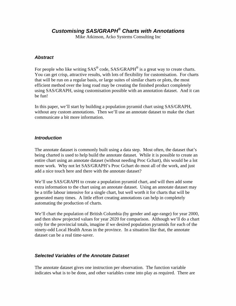
Selected Variables of the Annotate Dataset The annotate dataset gives one instruction per observation. The function variable indicates what is to be done, and other variables come into play as required. There are

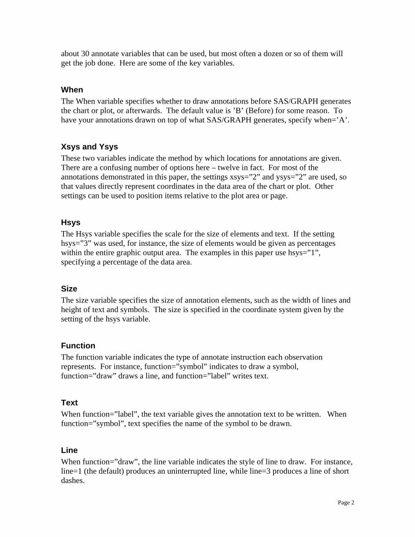
about 30 annotate variables that can be used, but most often a dozen or so of them will get the job done. Here are some of the key variables.

When The When variable specifies whether to draw annotations before SAS/GRAPH generates the chart or plot, or afterwards. The default value is ’B’ (Before) for some reason. To have your annotations drawn on top of what SAS/GRAPH generates, specify when=’A’.

Xsys and Ysys These two variables indicate the method by which locations for annotations are given. There are a confusing number of options here – twelve in fact. For most of the annotations demonstrated in this paper, the settings xsys=”2” and ysys=”2” are used, so that values directly represent coordinates in the data area of the chart or plot. Other settings can be used to position items relative to the plot area or page.

Hsys The Hsys variable specifies the scale for the size of elements and text. If the setting hsys=”3” was used, for instance, the size of elements would be given as percentages within the entire graphic output area. The examples in this paper use hsys=”1”, specifying a percentage of the data area.

Size The size variable specifies the size of annotation elements, such as the width of lines and height of text and symbols. The size is specified in the coordinate system given by the setting of the hsys variable.

Function The function variable indicates the type of annotate instruction each observation represents. For instance, function=”symbol” indicates to draw a symbol, function=”draw” draws a line, and function=”label” writes text.

Text When function=”label”, the text variable gives the annotation text to be written. When function=”symbol”, text specifies the name of the symbol to be drawn.

Line When function=”draw”, the line variable indicates the style of line to draw. For instance, line=1 (the default) produces an uninterrupted line, while line=3 produces a line of short dashes.

Page 2

Color Color can be specified in various ways: by name, by RGB value, by CMYK, HLS, gray-scale, or other methods. For straightforward colors, it is easiest use the color names such as “black” and “white”. When finer control is desired, you may choose to supply RGB values, or use one of the other methods. Here is a typical RGB value representing a very light purple: color=”cxCB74D9”. The cx at the start indicates that an RGB value is being given, and the remainder are pairs of hexadecimal digits representing the amount of red (CB), green (74) and blue (D9).

Midpoint, Group, & Subgroup The midpoint variable works with the coordinate system given by xsys=”2” and ysys=”2”, and with a few other coordinate systems. Midpoint is an alternative to using either variable x or variable y, depending upon which type of chart is being produced. For instance, in a VBAR chart, you would probably position annotations using Midpoint in conjunction with variable Y. Midpoint would indicate which bar you are annotating, with Y indicating the position along the bar. If the chart used the group= or subgroup= option in the vbar or hbar statement, you can use the corresponding variable(s) (group and subgroup) along with the midpoint variable. These variable(s) (along with midpoint) indicate which bar to annotate, and either X or Y would be used to specify a location relative to the height of the bar. Unlike the X and Y variables, which always specify numeric coordinates relative to one of the axes, the Midpoint (and group and subgroup) variable(s) supply values (or formatted values) corresponding to bars in the chart. Basing the annotate dataset on the same dataset that is being charted makes it easy; the Midpoint variable can be set to the value of the variable that is being charted. For instance, midpoint=age_range;

X & Y In a bar chart, the midpoint variable specifies position along one of the axes, and the other is specified by either X or Y. In a plot, both X and Y are used for positioning annotation elements. With Xsys=”2” (and/or Ysys=”2”), the data values of the X or Y variable(s) can be used to position annotations.

Position The Position variable is used only to specify how text (via function=”label”) is to be placed, in relation to the point identified by variables Midpoint, X, Y, etc. Given a point on the chart, the setting of the Position variable can be used to centre the text there, or to left or right adjust the text relative to the point. The Position variable can be set to one of “1” to “9”, “A” to “F”, “<”, “+”, “>”, or “0”.

Page 3

Style The Style variable specifies the font for labels and symbols (if you want to depart from the default font). Style can also indicate the method for filling objects like bars and pie slices.

Other variables There are many other variables, some of which are used in this paper. Include additional variables as required; unused variables do not need to appear in the annotate dataset.

Sample Population Pyramid Chart It is possible to have SAS/GRAPH create a nice population pyramid chart with minimal effort on the programmer’s part. In this paper, a horizontal bar chart is created using Proc Gchart and the Hbar statement. To get bars for Female and Male to both the left and right of the vertical axis, we can set the values for one of the genders to negative. For this chart, annual population figures for British Columbia (by age-range and gender) were found on the BC Stats web page: <http://www.bcstats.gov.bc.ca/DATA/POP/pop/project/BCtab_Proj0901.pdf>. These were read into SAS and transposed into a dataset with the variables Year, Gender, Age_Range, and Popn. To create the population pyramid (with female values going left and male values right of the center axis) the population figures for females were made negative by subtracting each value from zero. A format (called thousand) was created and used in the Proc Gchart so that the artificially negative values look correct (i.e. positive) when written. By default, Proc Gchart would show age ranges in ascending order (from top to bottom), creating a population tree instead of a population pyramid. (Population trees show the population of younger people at the top and more elderly at the bottom, while population pyramids are the other way around.) Although both types of chart are in fairly common use, the population pyramid is seen a bit more often. To change to a pyramid, age range values were made into a list in descending order using Proc SQL, and this list was given in the midpoints option of the Hbar statement. The code to produce a (rather spare) population pyramid is below.

Page 4

* We’ll chart population for a single year; %let year1 = 2000; * Create a format for showing negative values as if they were positive; * (Show values in thousands, with one decimal); proc format; picture thousand low-high = '0,000.0K' (mult=0.01); run; * Get a list of the age ranges in descending order (for midpoint list); * Put quotes around values (except for the very first and last quotes); proc sql noprint; select distinct age_range into :age_ranges separated by '" "' from bc_people where year = &year1 order by age_range desc; quit; * Population Pyramid Chart for BC; axis1 label=(j=c angle=90 h=12pt 'Age Range') style=1 width=3 value=(h=12pt); axis2 label=none style=1 width=3 value=(angle=0 rotate=0 h=12pt) order=(-200000 to 200000 by 50000); pattern1 value=solid color=cxCB74D9; * Very Light Purple; pattern2 value=solid color=cx13478C; * Vivid Greenish Blue; proc gchart data=bc_people; where year = &year1; hbar age_range / sumvar = popn subgroup = gender midpoints = "&age_ranges" maxis = axis1 raxis = axis2 autoref nostats nolegend; format popn thousand.; title1 h=14pt "BC Population Pyramid for &year1"; footnote1 j=l h=9pt f="Helvetica" "Source: BC Stats <http://www.bcstats.gov.bc.ca/DATA/POP/pop/project/BCtab_Proj0901.pdf>"; run; quit;

Page 5

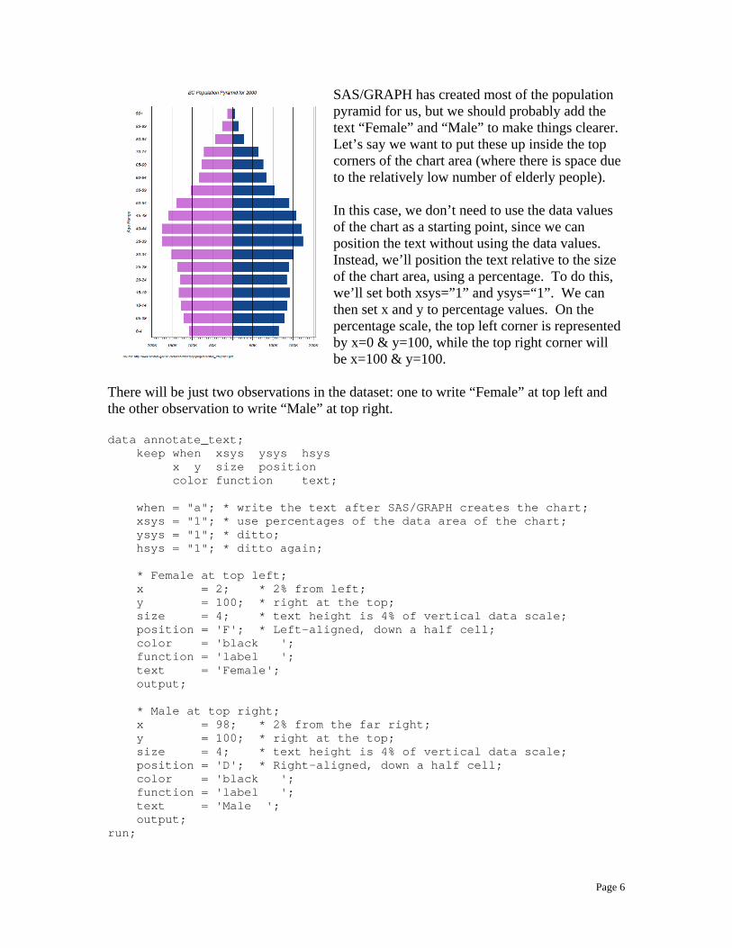
SAS/GRAPH has created most of the population pyramid for us, but we should probably add the text “Female” and “Male” to make things clearer. Let’s say we want to put these up inside the top corners of the chart area (where there is space due to the relatively low number of elderly people). In this case, we don’t need to use the data values of the chart as a starting point, since we can position the text without using the data values. Instead, we’ll position the text relative to the size of the chart area, using a percentage. To do this, we’ll set both xsys=”1” and ysys=“1”. We can then set x and y to percentage values. On the percentage scale, the top left corner is represented by x=0 & y=100, while the top right corner will be x=100 & y=100.

There will be just two observations in the dataset: one to write “Female” at top left and the other observation to write “Male” at top right. data annotate_text; keep when xsys ysys hsys x y size position color function text; when = "a"; * write the text after SAS/GRAPH creates the chart; xsys = "1"; * use percentages of the data area of the chart; ysys = "1"; * ditto; hsys = "1"; * ditto again; * Female at top left; x = 2; * 2% from left; y = 100; * right at the top; size = 4; * text height is 4% of vertical data scale; position = 'F'; * Left-aligned, down a half cell; color = 'black '; function = 'label '; text = 'Female'; output; * Male at top right; x = 98; * 2% from the far right; y = 100; * right at the top; size = 4; * text height is 4% of vertical data scale; position = 'D'; * Right-aligned, down a half cell; color = 'black '; function = 'label '; text = 'Male '; output; run;

Page 6

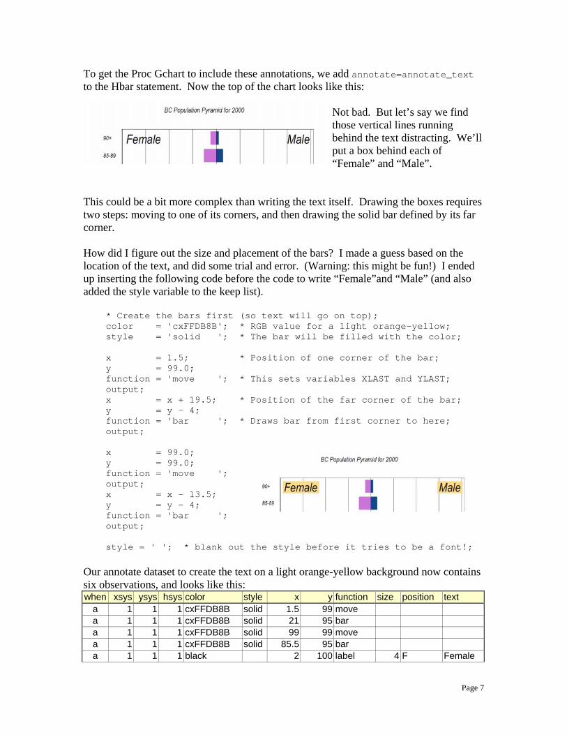
To get the Proc Gchart to include these annotations, we add annotate=annotate_text to the Hbar statement. Now the top of the chart looks like this:

” and “Male”.

Not bad. But let’s say we findthose vertical lines running behind the text distracting. We’ll put a box behind each of “Female

This could be a bit more complex than writing the text itself. Drawing the boxes requires two steps: moving to one of its corners, and then drawing the solid bar defined by its far corner. How did I figure out the size and placement of the bars? I made a guess based on the location of the text, and did some trial and error. (Warning: this might be fun!) I ended up inserting the following code before the code to write “Female”and “Male” (and also added the style variable to the keep list). * Create the bars first (so text will go on top); color = 'cxFFDB8B'; * RGB value for a light orange-yellow; style = 'solid '; * The bar will be filled with the color; x = 1.5; * Position of one corner of the bar; y = 99.0; function = 'move '; * This sets variables XLAST and YLAST; output; x = x + 19.5; * Position of the far corner of the bar; y = y - 4; function = 'bar '; * Draws bar from first corner to here; output; x = 99.0; y = 99.0; function = 'move '; output; x = x - 13.5; y = y - 4; function = 'bar '; output; style = ' '; * blank out the style before it tries to be a font!; Our annotate dataset to create the text on a light orange-yellow background now contains six observations, and looks like this: when xsys ysys hsys color style x y function size position text

a 1 1 1 cxFFDB8B solid 1.5 99 move a 1 1 1 cxFFDB8B solid 21 95 bar a 1 1 1 cxFFDB8B solid 99 99 move a 1 1 1 cxFFDB8B solid 85.5 95 bar a 1 1 1 black 2 100 label 4 F Female

Page 7

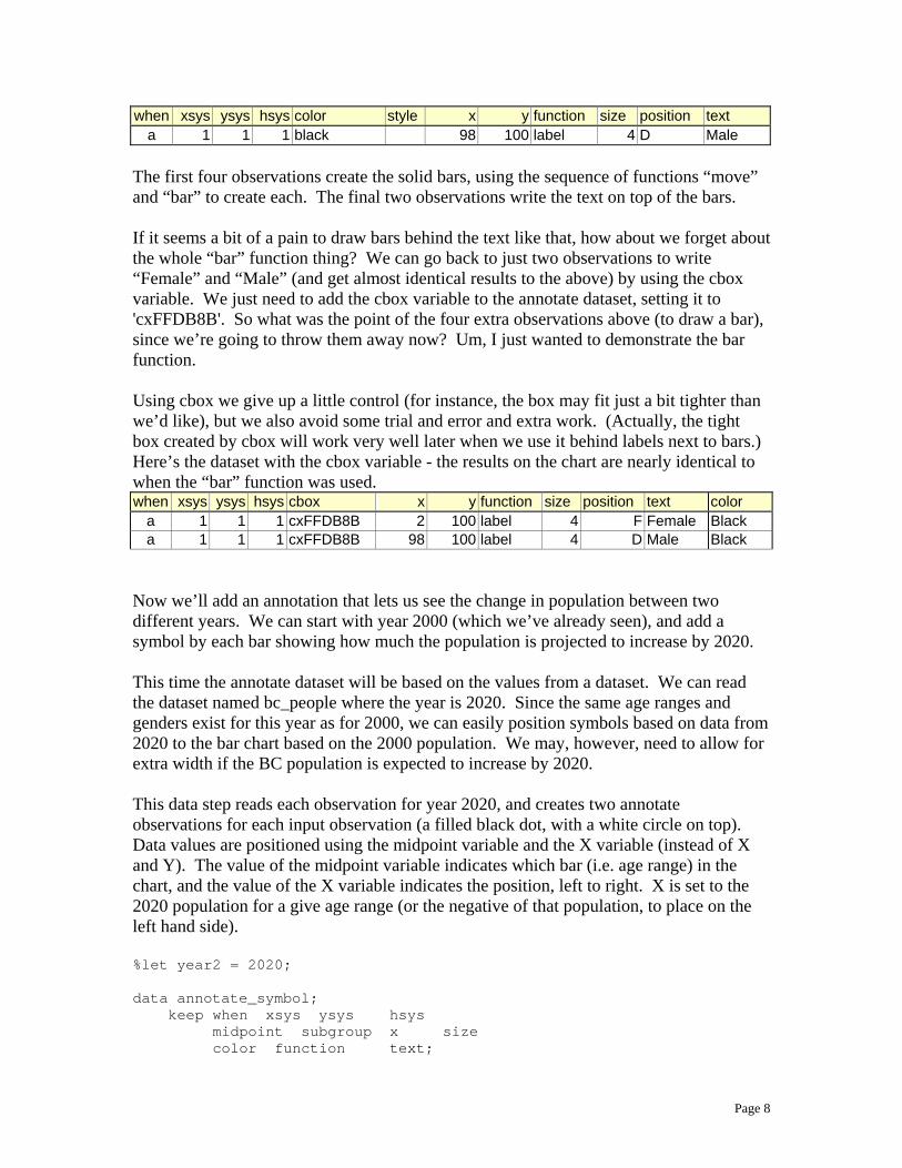
when xsys ysys hsys color style x y function size position text a 1 1 1 black 98 100 label 4 D Male

The first four observations create the solid bars, using the sequence of functions “move” and “bar” to create each. The final two observations write the text on top of the bars. If it seems a bit of a pain to draw bars behind the text like that, how about we forget about the whole “bar” function thing? We can go back to just two observations to write “Female” and “Male” (and get almost identical results to the above) by using the cbox variable. We just need to add the cbox variable to the annotate dataset, setting it to 'cxFFDB8B'. So what was the point of the four extra observations above (to draw a bar), since we’re going to throw them away now? Um, I just wanted to demonstrate the bar function. Using cbox we give up a little control (for instance, the box may fit just a bit tighter than we’d like), but we also avoid some trial and error and extra work. (Actually, the tight box created by cbox will work very well later when we use it behind labels next to bars.) Here’s the dataset with the cbox variable - the results on the chart are nearly identical to when the “bar” function was used. when xsys ysys hsys cbox x y function size position text color

a 1 1 1 cxFFDB8B 2 100 label 4 F Female Black a 1 1 1 cxFFDB8B 98 100 label 4 D Male Black

Now we’ll add an annotation that lets us see the change in population between two different years. We can start with year 2000 (which we’ve already seen), and add a symbol by each bar showing how much the population is projected to increase by 2020. This time the annotate dataset will be based on the values from a dataset. We can read the dataset named bc_people where the year is 2020. Since the same age ranges and genders exist for this year as for 2000, we can easily position symbols based on data from 2020 to the bar chart based on the 2000 population. We may, however, need to allow for extra width if the BC population is expected to increase by 2020. This data step reads each observation for year 2020, and creates two annotate observations for each input observation (a filled black dot, with a white circle on top). Data values are positioned using the midpoint variable and the X variable (instead of X and Y). The value of the midpoint variable indicates which bar (i.e. age range) in the chart, and the value of the X variable indicates the position, left to right. X is set to the 2020 population for a give age range (or the negative of that population, to place on the left hand side). %let year2 = 2020; data annotate_symbol; keep when xsys ysys hsys midpoint subgroup x size color function text;

Page 8

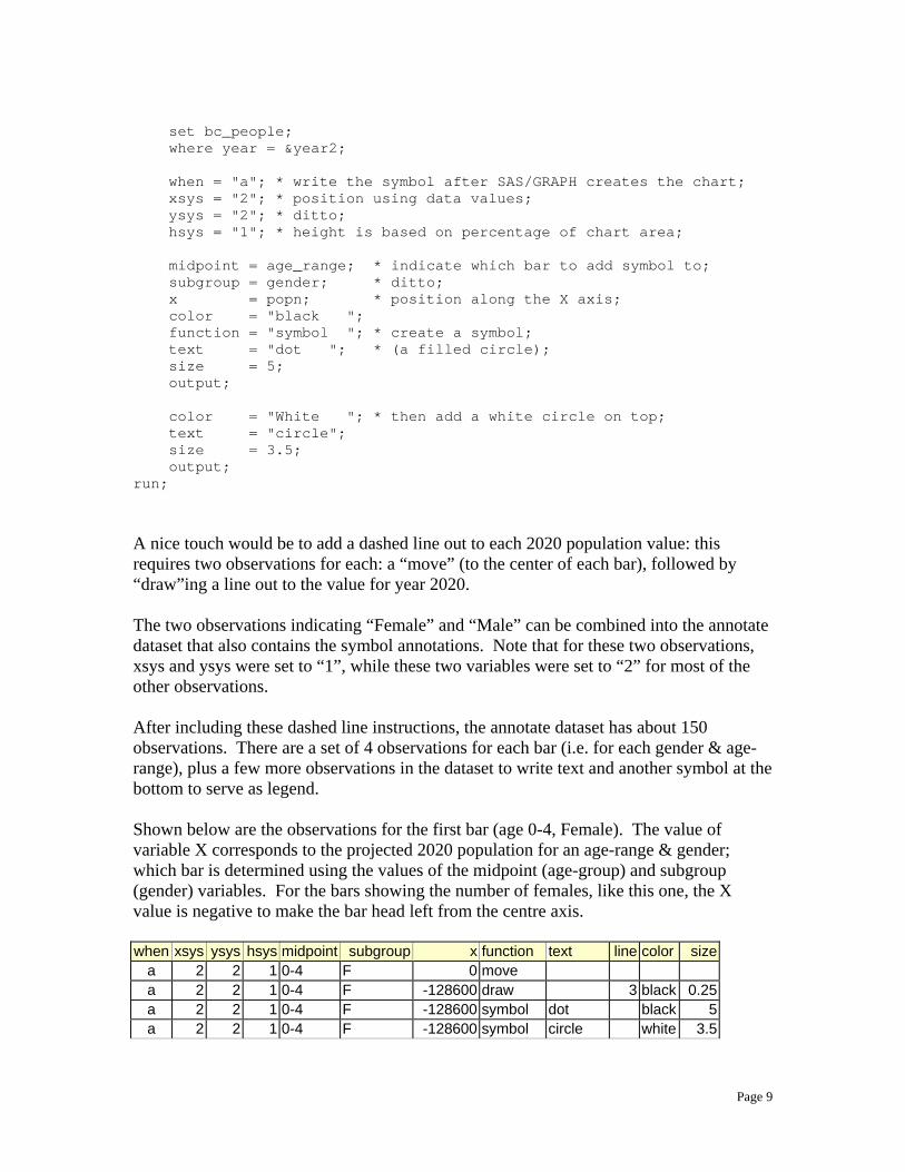
set bc_people; where year = &year2; when = "a"; * write the symbol after SAS/GRAPH creates the chart; xsys = "2"; * position using data values; ysys = "2"; * ditto; hsys = "1"; * height is based on percentage of chart area; midpoint = age_range; * indicate which bar to add symbol to; subgroup = gender; * ditto; x = popn; * position along the X axis; color = "black "; function = "symbol "; * create a symbol; text = "dot "; * (a filled circle); size = 5; output; color = "White "; * then add a white circle on top; text = "circle"; size = 3.5; output; run; A nice touch would be to add a dashed line out to each 2020 population value: this requires two observations for each: a “move” (to the center of each bar), followed by “draw”ing a line out to the value for year 2020. The two observations indicating “Female” and “Male” can be combined into the annotate dataset that also contains the symbol annotations. Note that for these two observations, xsys and ysys were set to “1”, while these two variables were set to “2” for most of the other observations. After including these dashed line instructions, the annotate dataset has about 150 observations. There are a set of 4 observations for each bar (i.e. for each gender & age-range), plus a few more observations in the dataset to write text and another symbol at the bottom to serve as legend. Shown below are the observations for the first bar (age 0-4, Female). The value of variable X corresponds to the projected 2020 population for an age-range & gender; which bar is determined using the values of the midpoint (age-group) and subgroup (gender) variables. For the bars showing the number of females, like this one, the X value is negative to make the bar head left from the centre axis. when xsys ysys hsys midpoint subgroup x function text line color size

a 2 2 1 0-4 F 0 move a 2 2 1 0-4 F -128600 draw 3 black 0.25 a 2 2 1 0-4 F -128600 symbol dot black 5 a 2 2 1 0-4 F -128600 symbol circle white 3.5

Page 9

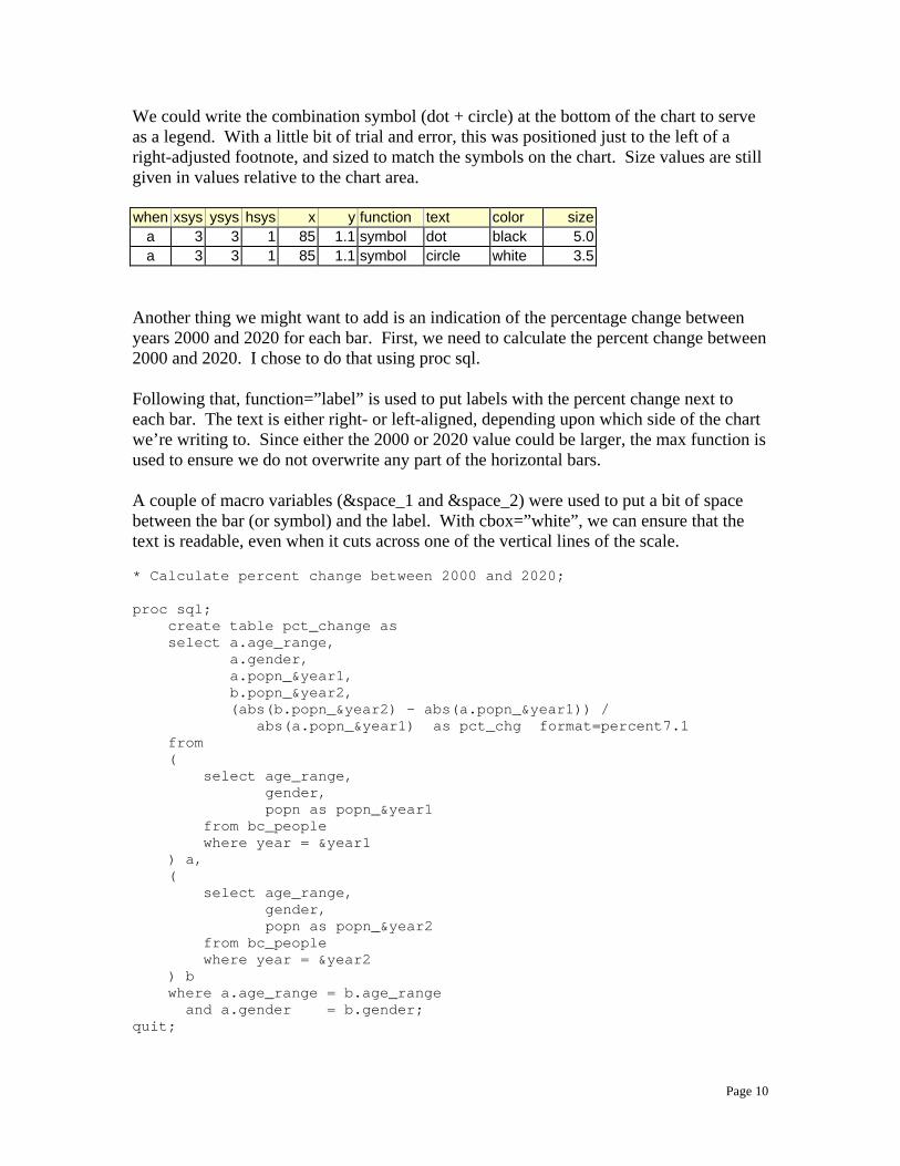
We could write the combination symbol (dot + circle) at the bottom of the chart to serve as a legend. With a little bit of trial and error, this was positioned just to the left of a right-adjusted footnote, and sized to match the symbols on the chart. Size values are still given in values relative to the chart area. when xsys ysys hsys x y function text color size

a 3 3 1 85 1.1 symbol dot black 5.0a 3 3 1 85 1.1 symbol circle white 3.5

Another thing we might want to add is an indication of the percentage change between years 2000 and 2020 for each bar. First, we need to calculate the percent change between 2000 and 2020. I chose to do that using proc sql. Following that, function=”label” is used to put labels with the percent change next to each bar. The text is either right- or left-aligned, depending upon which side of the chart we’re writing to. Since either the 2000 or 2020 value could be larger, the max function is used to ensure we do not overwrite any part of the horizontal bars. A couple of macro variables (&space_1 and &space_2) were used to put a bit of space between the bar (or symbol) and the label. With cbox=”white”, we can ensure that the text is readable, even when it cuts across one of the vertical lines of the scale. * Calculate percent change between 2000 and 2020; proc sql; create table pct_change as select a.age_range, a.gender, a.popn_&year1, b.popn_&year2, (abs(b.popn_&year2) - abs(a.popn_&year1)) / abs(a.popn_&year1) as pct_chg format=percent7.1 from ( select age_range, gender, popn as popn_&year1 from bc_people where year = &year1 ) a, ( select age_range, gender, popn as popn_&year2 from bc_people where year = &year2 ) b where a.age_range = b.age_range and a.gender = b.gender; quit;

Page 10

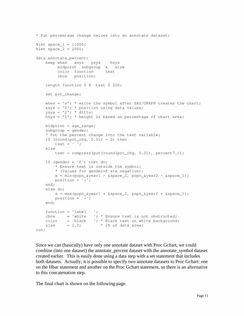
* Put percentage change values into an annotate dataset; %let space_1 = 11000; %let space_2 = 2000; data annotate_percent; keep when xsys ysys hsys midpoint subgroup x size color function text cbox position; length function $ 8 text $ 200; set pct_change; when = "a"; * write the symbol after SAS/GRAPH creates the chart; xsys = "2"; * position using data values; ysys = "2"; * ditto; hsys = "1"; * height is based on percentage of chart area; midpoint = age_range; subgroup = gender; * Put the percent change into the text variable; if (round(pct_chg, 0.01) = 0) then text = ' '; else text = compress(put(round(pct_chg, 0.01), percent7.)); if (gender = 'F') then do; * Ensure text is outside the symbol; * (Values for gender=F are negative); x = min(popn_&year1 - &space_2, popn_&year2 - &space_1); position = '<'; end; else do; x = max(popn_&year1 + &space_2, popn_&year2 + &space_1); position = '>'; end; function = 'label '; cbox = 'white '; * Ensure text is not obstructed; color = 'black '; * Black text on white background; size = 2.0; * 2% of data area; run; Since we can (basically) have only one annotate dataset with Proc Gchart, we could combine (into one dataset) the annotate_percent dataset with the annotate_symbol dataset created earlier. This is easily done using a data step with a set statement that includes both datasets. Actually, it is possible to specify two annotate datasets to Proc Gchart: one on the Hbar statement and another on the Proc Gchart statement, so there is an alternative to this concatenation step. The final chart is shown on the following page.

Page 11

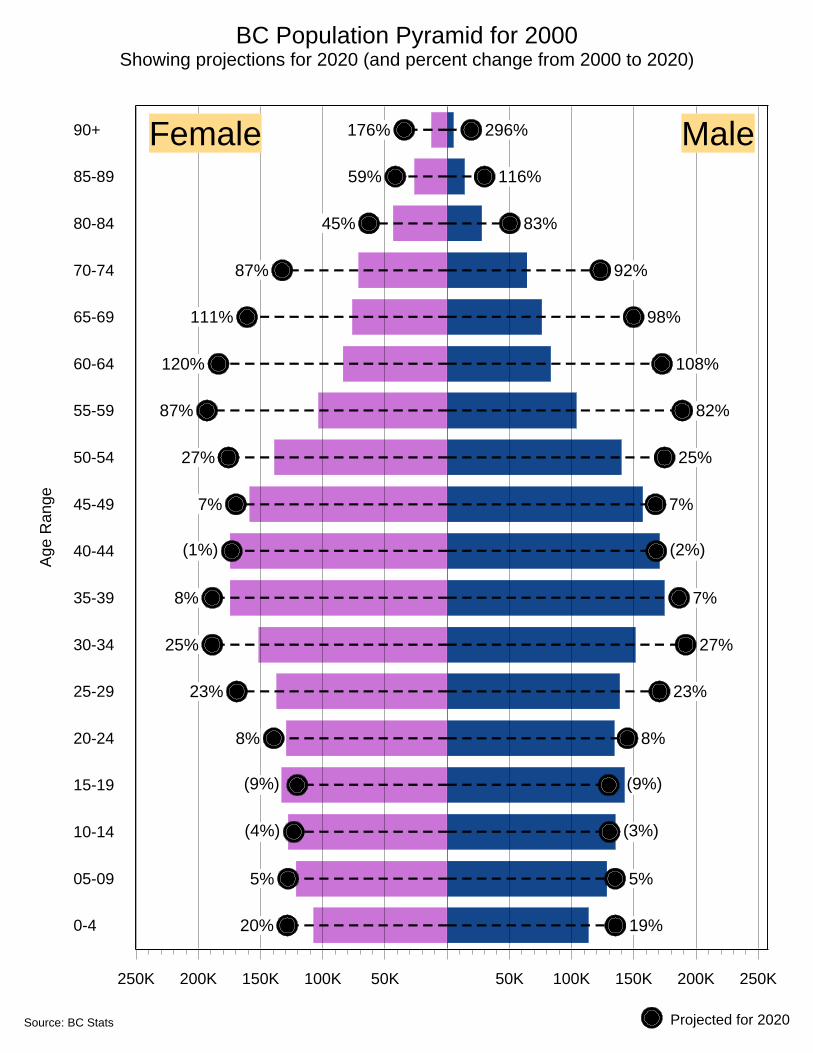
BC Population Pyramid for 2000Showing projections for 2020 (and percent change from 2000 to 2020)

Source: BC Stats Projected for 2020

Age

Ran

ge

0-4

05-09

10-14

15-19

20-24

25-29

30-34

35-39

40-44

45-49

50-54

55-59

60-64

65-69

70-74

80-84

85-89

90+

250K 200K 150K 100K 50K 50K 100K 150K 200K 250K

Female Male

20%

5%

(4%)

(9%)

8%

23%

25%

8%

(1%)

7%

27%

87%

120%

111%

87%

45%

59%

176%

19%

5%

(3%)

(9%)

8%

23%

27%

7%

(2%)

7%

25%

82%

108%

98%

92%

83%

116%

296%

Conclusion The annotate dataset is great for adding customisation to SAS/GRAPH charts, especially if you like writing SAS code. Custom additions of text, symbols (and more) to charts can be accomplished by adding instructions/observations to the annotate dataset. This can be a great time-saver when a large number of similar charts are to be produced.

Contact Information Mike Atkinson Acko Systems Consulting Inc (250) 208-6908 acko@telus.net

SAS and all other SAS Institute Inc. product or service names are registered trademarks or trademarks of SAS Institute Inc. in the USA and other countries. ® indicates USA registration. Other brand and product

names are registered trademarks or trademarks of their respective companies.

Page 13