Curvilinear Coordinates

By

Al Bernstein Signal Science, LLC

www.signalscience.net alb@signalscience.net

Introduction

Curvilinear coordinates are local coordinate systems defined on a manifold – a generalization of

a surface. A surface is a 2-D manifold. A manifold is defined as a topological space that is

Euclidean (flat) a small distance around each point. A differentiable manifold is a manifold

where calculus is valid. Cartesian coordinates are considered a global coordinate system because

the axes defining the coordinate system remain fixed. In local coordinate systems the axes

change based on the position.

Vectors

The concept of vector on a manifold is different than the usual definition because a manifold

behaves like a Euclidean coordinate system an infinitesimal distance around each point. The

basis vectors of a local coordinate system at each point of a manifold are defined by derivatives

because a derivative brings two points an infinitesimal distance from each other to create a

tangent vector. Figure 1 shows what would happen if a vector is drawn along the curve – it is an

arc with an arrow. This object does not behave as a vector.

Figure 1

P

ɵ

Figure 2 shows how a vector is created by a derivative. The right side is a magnified picture of

the left side and shows that a vector is defined by the slope and direction from 𝑓(𝑥) to 𝑓(𝑥 + ℎ).

Figure 2

Equation (1) shows the definition of derivative in the limit as a slope for ℎ → 0.

𝑑𝑓

𝑑𝑥= lim

ℎ→0

𝑓(𝑥 + ℎ) − 𝑓(𝑥)

ℎ

(1)

So the Tangent Vector to 𝒇(𝒙) at x ≡𝒅𝒇(𝒙)

𝒅𝒙

• • 𝑓(𝑥)

𝑓(𝑥 + ℎ)

𝑥 • • 𝑥 + ℎ

𝑥 𝑥 + ℎ

𝑓(𝑥)

𝑓(𝑥 + ℎ)

𝑑𝑥

𝑑𝑓

Figure 3

Figure 3 shows that the tangent to the curve at point P and a tangent along the radius are vectors

and can be thought of as a coordinate system. Tangent vectors are defined as derivatives as

shown above and define local coordinates at P. Since P can be anywhere on the curve, the

tangent vectors [𝜕𝑃

𝜕𝑟,𝜕𝑃

𝜕𝜃] are defined by equation (2) and are the polar coordinate basis vectors.

𝑒𝑟 =𝜕

𝜕𝑟

𝑒𝜃 =𝜕

𝜕𝜃

(2)

Note: when the coordinates such as those in Figure 3 are used, their offset is removed – their

origin is moved to the origin in the Cartesian coordinate system.

General Vector Coordinate Transformations

Consider a polar coordinate system.

𝑥 = 𝑟𝑐𝑜𝑠(𝜃) (3)

𝑦 = 𝑟𝑠𝑖𝑛(𝜃)

To find how the basis vectors transform, use the chain rule as follows.

Equation (4) and (5) use the chain rule to define the polar coordinate basis vectors in terms of the

Cartesian basis vectors.

𝜕𝑃

𝜕𝑟

P

𝜕𝑃

𝜕𝜃

𝜕

𝜕𝑟=

𝜕𝑥

𝜕𝑟

𝜕

𝜕𝑥+

𝜕𝑦

𝜕𝑟

𝜕

𝜕𝑦

(4)

𝜕

𝜕𝜃=

𝜕𝑥

𝜕𝜃

𝜕

𝜕𝑥+

𝜕𝑦

𝜕𝜃

𝜕

𝜕𝑦

(5)

where 𝜕

𝜕𝑥 and

𝜕

𝜕𝑦 are the basis vectors in Cartesian coordinates

Equations (4) and (5) can be viewed in matrix notation as

𝜕

𝜕𝒀=

𝜕𝑿

𝜕𝒀

𝜕

𝜕𝑿

(6)

where 𝒀 = [𝑟 𝜃] , 𝑿 = [𝑥 𝑦] and

𝜕𝑿

𝜕𝒀= [

𝜕𝑥

𝜕𝑟

𝜕𝑦

𝜕𝑟𝜕𝑥

𝜕𝜃

𝜕𝑦

𝜃

]

Equation (6) is nice because 𝑿 and 𝒀 can be any coordinate system.

Expanding equation (4) and (5) from equation (3) gives equations (7).

𝜕

𝜕𝑟= cos(𝜃)

𝜕

𝜕𝑥+ sin (𝜃)

𝜕

𝜕𝑦

𝜕

𝜕𝜃= −𝑟𝑠𝑖𝑛(𝜃)

𝜕

𝜕𝑥+ 𝑟𝑐𝑜𝑠(𝜃)

𝜕

𝜕𝑦

(7)

The transformation in matrix form is given by equation (8).

�̅� = 𝐴(𝑟, 𝜃)𝑒 = [

𝜕

𝜕𝑟𝜕

𝜕𝜃

] = 𝐴(𝑟, 𝜃) ∙

[

𝜕

𝜕𝑥𝜕

𝜕𝑦]

= 𝜕𝑿

𝜕𝒀∙

[

𝜕

𝜕𝑥𝜕

𝜕𝑦]

= [cos (𝜃) 𝑠𝑖𝑛(𝜃)

−rsin (𝜃) 𝑟𝑐𝑜𝑠(𝜃)] ∙

[

𝜕

𝜕𝑥𝜕

𝜕𝑦]

(8)

Suppose 𝜃 =𝜋

4 and 𝑟 = 1, then from (8) the polar coordinate basis functions in terms of the

Cartesian basis vectors are

�̅�1 =𝜕

𝜕𝑟=

1

√2

𝜕

𝜕𝑥+

1

√2

𝜕

𝜕𝑦

(9)

�̅�2 =𝜕

𝜕𝜃=

−1

√2

𝜕

𝜕𝑥+

1

√2

𝜕

𝜕𝑦

(10)

Transforming a vector 𝑣 = [1 0] to the polar coordinate system �̅� is shown below.

�̅� = 𝐴 (1,𝜋

4) 𝑣 = [

1√2

⁄ 1√2

⁄

−1√2

⁄ 1√2

⁄] [

10] = [

1√2

⁄

−1√2

⁄]

(11)

Multiplying the polar basis functions by the vector values gives

�̅�1�̅�1 + �̅�2�̅�2 = (1√2

⁄ ) [

1√2

⁄

1√2

⁄] − (1

√2⁄ ) [

− 1√2

⁄

1√2

⁄] = [

10]

(12)

which is what we would expect!

Let’s repeat the same process with 𝑟 = 2. The basis functions are now

�̅�1 =1

√2

𝜕

𝜕𝑥+

1

√2

𝜕

𝜕𝑦

(13)

�̅�2 = −√2𝜕

𝜕𝑥+ √2

𝜕

𝜕𝑦

(14)

�̅� = 𝐴 (2,𝜋

4) 𝑣 = [

1√2

⁄ 1√2

⁄

−√2 √2] [

10] = [

1√2

⁄

−√2]

(15)

�̅�1�̅�1 + �̅�2�̅�2 = (1√2

⁄ ) [

1√2

⁄

1√2

⁄] − √2 [−√2

√2] = [

1

2+ 2

1

2− 2

] = [5

2⁄

−32⁄] ≠ [

10]

(16)

Equation (16) shows that in the general case, the vector components don’t transform using

equation (8).

The next step is to find how the vector components transform. Equations (17) and (18) show a

general transform for the basis vectors and vector components

�̅� = 𝐴𝑒 (17)

�̅� = 𝐵𝑣 (18)

The unknown 𝐵 matrix transforms the components of 𝑣 from the 𝑒 to �̅� coordinate system.

Since 𝑣 is fixed in space - coordinate systems are changing – equation (19) must hold.

Multiplying the components of �̅� out in the transformed coordinate system must produce the

components of 𝑣 in the original coordinate system.

�̅� ∙ �̅� = 𝑒 ∙ 𝑣 = 𝑣 (19)

In matrix notation �̅� ∙ �̅� ≡ �̅�𝑇�̅�

�̅�𝑇�̅� = [𝐴𝑒]𝑇𝐵𝑣 = 𝑒𝑇𝐴𝑇𝐵𝑣 = 𝑒𝑇𝑣 (20)

So

𝐴𝑇𝐵 = 𝐼 → 𝐵 = (𝐴𝑇)−1 = (𝐴−1)𝑇 (21)

Equation (21) shows that the vector components transform using 𝐵 = (𝐴𝑇)−1 while the basis vectors

transform using 𝐴.

Box 1

Vector Components Transform

Differently Than Their Bases in

the General Case

Box 2

Basis Vectors Transform Using Matrix 𝑨

Vector Components Transform Using 𝑩 = (𝑨𝑻)−𝟏

𝐵(𝑟, 𝜃) = [𝐴(𝑟, 𝜃)𝑇]−1 = [cos (𝜃) 𝑠𝑖𝑛(𝜃)−sin (𝜃)

𝑟

𝑐𝑜𝑠(𝜃)

𝑟

] (22)

�̅� = 𝐵 (2,𝜋

4) 𝑣 = [

1√2

⁄ 1√2

⁄

−12

32⁄⁄ 1

23

2⁄⁄] [

10] = [

1√2

⁄

−12

32⁄⁄] (23)

�̅�1�̅�1 + �̅�2�̅�2 = (1√2

⁄ ) [

1√2

⁄

1√2

⁄] − (1

23

2⁄⁄ ) [−√2

√2] = [

12⁄

12⁄] − [

−12⁄

12⁄

] = [10] (24)

Now we get the correct answer!

A vector will be denoted as

𝑣 = 𝑣𝑥𝑒𝑥 + 𝑣𝑦𝑒𝑦 + ⋯

(25)

where 𝑣𝑖 are the vector components and

𝑒𝑖 =𝜕

𝜕𝑥𝑖

(26)

We know that the basis vectors 𝑒𝑖 transform using 𝐴(𝑟, 𝜃) and the vector components 𝑣𝑖 transform

using 𝐵(𝑟, 𝜃). Let’s try to take the dot product of two vectors by transforming the vector

components using 𝐵(𝑟, 𝜃). We know

𝐵 (2,𝜋

4) [

10] = [

1√2

⁄

−12

32⁄⁄]

We can use [32] as the second vector

𝐵 (2,𝜋

4) [

32] = [

1√2

⁄ 1√2

⁄

−12

32⁄⁄ 1

23

2⁄⁄] [

32] = [

5√2

⁄

−12

32⁄⁄]

(27)

The dot product now is [1

√2⁄ −1

23

2⁄⁄ ]

[

5√2

⁄

−12

32⁄⁄

]

=5

2+

1

8=

21

8≠ [1 0] [

32] = 3 (28)

So we cannot use 𝐵(𝑟, 𝜃) to transform both vectors – but the vector components transform using

𝐵(𝑟, 𝜃). We need a new type of math construct that gives the correct dot product in the general

case.

Equation (29) shows how the components of this new construct transform.

�̅� = 𝐶𝛼 (29)

We know that

�̅� = 𝐵𝑣 (30)

Now equation (31) must hold to keep the dot product the same in all coordinate systems.

�̅� ∙ �̅� = 𝛼 ∙ 𝑣 = 𝑐𝑜𝑛𝑠𝑡𝑎𝑛𝑡 (31)

Substituting equations (29) and (30) into equation (31) gives equations (32) and (33).

�̅�𝑇�̅� = [𝐶𝛼]𝑇𝐵𝑣 = 𝛼𝑣 (32)

𝛼𝑇𝐶𝑇𝐵𝑣 = 𝛼𝑇𝑣 (33)

So

𝐶𝑇𝐵 = 𝐼

𝐵 = (𝐶𝑇)−1 = (𝐴𝑇)−1

So 𝐶 = 𝐴

So the new constructs components transform as

�̅� = 𝐴𝛼 (34)

To test, transform one of the vectors using 𝐴 (2,𝜋

4)

Box 3

A New Math Construct is Needed to Compute the Inner

Product

𝐴 (2,𝜋

4) [

32] = [

1√2

⁄ 1√2

⁄

−√2 √2] [

32] = [

5√2

⁄

−√2] (35)

The dot product now is [5√2

⁄ −√2]

[

1√2

⁄

−12

32⁄⁄

]

= 52⁄ + 1

2⁄ = [1 0] [32] = 3

We get the correct answer!

Differential 1 Forms

Differential 1-Forms are less known than vectors. They are any expression involving a linear

combination of single differentials. For example 𝐴𝑑𝑥 + 𝐵𝑑𝑦 is a differential 1 form. Differential

1 forms in 2-D are lines because 𝑎𝑥 + 𝑏𝑦 = 𝑐 is the equation of a line – 𝐴𝑑𝑥 are lines parallel to

the y axis, 𝐵𝑑𝑦 are lines parallel to the x axis, 𝑑𝑥 + 𝑑𝑦 are lines perpendicular to a line at a 45

degree angle.

In 3-D, differential 1 forms 𝐴𝑑𝑥 + 𝐵𝑑𝑦 + 𝐶𝑑𝑧 are visualized as planes because the equation for

a plane is 𝑎𝑥 + 𝑏𝑦 + 𝑐𝑧 = 𝑑. In 3-D, 𝐴𝑑𝑥 are planes parallel to the y-z plane, 𝐵𝑑𝑦 are planes

parallel to the x-z plane, and 𝐶𝑑𝑧 are planes parallel to the x-y plane.

A plane – (line) - can be characterized by a vector normal to the plane – (line) Using normal

vectors allows visualization of 1 forms as vectors – see figures 3 and 4 below

Box 4

This new construct is called a covector or a

differential 1 Form.

Figure 3

Figure 4

𝑥

𝑦

𝑑𝑥

𝑑𝑦

𝑑𝑥 + 𝑑𝑦

𝑥

𝑦

The normal vectors of differential forms show that 1 – Forms add like vectors – see Figure 5.

Figure 5

1 forms are numerically evaluated between two vectors. For example, 𝑑𝑥 + 2𝑑𝑦 + 3𝑑𝑧

evaluated over

𝑣1 = [1 2 1] and 𝑣2 = [3 6 5] is (3 − 1) + 2(6 − 2) + 3(5 − 1) = 2 +8 + 12 = 22

1 forms are usually used – as differentials - without numerically evaluating them.

In the language of differential forms, the basis 1 forms in polar coordinates are 𝑑𝑟 and 𝑑𝜃 – see

Figure 6.

Figure 6

𝑑𝑟 𝑑𝜃

𝑑𝑥

𝑑𝑦

𝑑𝑥 + 𝑑𝑦

Box 5

Normal Vectors of 1-Forms

Show 1-Forms Add Like Vectors

Comparing Figures 2 and 6, the reader may ask what the differences between one forms and

vectors are. The difference is that they transform differently.

In the last section, we showed that the coefficients of a differential 1-Form transform like

equation (34) – shown again below.

�̅� = 𝐴𝛼 (34)

To find out how the basis 1-Forms transform, start with equation (34) and (36)

�̅� = 𝐷𝜔 (36)

Using the same approach we used earlier

�̅� ∙ �̅� = 𝜔𝛼 → �̅�𝑇�̅� = 𝜔𝑇𝛼 (37)

𝜔𝑇𝐷𝑇𝐴𝛼 = 𝜔𝑇𝛼 → 𝐷 = (𝐴𝑇)−1 = 𝐵 (38)

Equations (39) and (40) show how the vector and 1-Forms basis sets transform.

�̅� = 𝐴𝑒 (39)

�̅� = 𝐵𝜔 (40)

We can see relationship between the vector and 1-Form basis sets by using the outer product. For

the following argument, we set 𝑒 and 𝜔 are in Cartesian Coordinates.

�̅� ⊗ �̅� (41)

In matrix notation

�̅��̅�𝑇 = 𝐴𝑒(𝐵𝜔)𝑇 = 𝐴𝑒𝜔𝑇𝐵𝑇 = 𝐴𝑒𝜔𝑇𝐴−1 = (42)

but

𝑒𝜔𝑇 =

[

𝜕

𝜕𝑥𝜕

𝜕𝑦]

[𝑑𝑥 𝑑𝑦] =

[ 𝑑𝑥

𝑑𝑥

𝑑𝑦

𝑑𝑥𝑑𝑥

𝑑𝑦

𝑑𝑦

𝑑𝑦]

= [1 00 1

]

(43)

Box 6

1-Form Coordinates Transform Using �̅� = 𝑨𝜶

1-Form Bases Transform using �̅� = 𝑩𝝎

where

𝑑𝑦

𝑑𝑥=

𝑑𝑦

𝑑𝑥= 0

because 𝑥 and 𝑦 are independent of each other

and

𝑑𝑥

𝑑𝑥=

𝑑𝑦

𝑑𝑦= 1

So

�̅��̅�𝑇 = 𝐴𝑒𝜔𝑇𝐴−1 = 𝐼 (44)

The dot product properties of [𝑑𝑟 𝑑𝜃] and [𝜕

𝜕𝑟

𝜕

𝜕𝜃] are shown in Table 1.

𝜕

𝜕𝑟∙ 𝑑𝑟 = 𝑑𝑟 ∙

𝜕

𝜕𝑟=

𝑑𝑟

𝑑𝑟= 1 𝜕

𝜕𝑟∙ 𝑑𝜃 = 𝑑𝜃 ∙

𝜕

𝜕𝑟=

𝑑𝜃

𝑑𝑟= 0

𝜕

𝜕𝜃∙ 𝑑𝑟 = 𝑑𝑟 ∙

𝜕

𝜕𝜃=

𝑑𝑟

𝑑𝜃= 0

𝜕

𝜕𝜃∙ 𝑑𝜃 = 𝑑𝜃 ∙

𝜕

𝜕𝜃=

𝑑𝜃

𝑑𝜗= 1

Table 1

We can use the chain rule on equation (2) to see that we get the matrix 𝐵(𝑟, 𝜃).

𝑥 = 𝑟𝑐𝑜𝑠(𝜃)

𝑦 = 𝑟𝑠𝑖𝑛(𝜃) (2)

𝑑𝑟 =𝜕𝑟

𝜕𝑥𝑑𝑥 +

𝜕𝑟

𝜕𝑦𝑑𝑦

(45)

𝑑𝜃 =𝜕𝜃

𝜕𝑥𝑑𝑥 +

𝜕𝜃

𝜕𝑦𝑑𝑦

(46)

𝑟(𝑥, 𝑦) = [𝑥2 + 𝑦2]1/2

(47)

𝜕

𝜕𝑟

𝜕

𝜕𝜃

𝑑𝑟 𝑑𝜃

𝜃(𝑥, 𝑦) = 𝑡𝑎𝑛−1 (𝑦

𝑥)

(48)

𝑑𝑟 = cos(𝜃) 𝑑𝑥 + sin(𝜃) 𝑑𝑦 (49)

𝑑𝜃 =−1

𝑟sin(𝜃) 𝑑𝑥 +

1

𝑟cos (𝜃)𝑑𝑦 (50)

Equation (51) shows equations (49) and (50) in matrix form.

[𝑑𝑟𝑑𝜃

] = [

cos (𝜃) 𝑠𝑖𝑛(𝜃)−sin (𝜃)

𝑟

𝑐𝑜𝑠(𝜃)

𝑟

] ∙ [𝑑𝑥𝑑𝑦

] = 𝐵(𝑟, 𝜃) [𝑑𝑥𝑑𝑦

]

(51)

The generalization of equations (45) and (46) can be represented using the matrix equation (52).

𝑑𝒀 = [𝜕𝒀

𝜕𝑿] 𝑑𝑿 =

[ 𝜕𝑟

𝜕𝑥

𝜕𝜃

𝜕𝑥𝜕𝑟

𝜕𝑦

𝜕𝜃

𝜕𝑦]

(52)

Comparing equation (52) with equations (45) and (46)

𝐵(𝑟, 𝜃) = [𝜕𝒀

𝜕𝑿]𝑇

So

[𝜕𝒀

𝜕𝑿]𝑇

[𝜕𝑿

𝜕𝒀] = 𝐼

(53)

A 1-Form will be denoted as

𝛼 = 𝛼𝑥𝜔𝑥 + 𝛼𝑦𝜔𝑦 + ⋯ (54)

where 𝛼𝑖 are the 1-form components and 𝜔𝑖 = 𝑑𝑥𝑖 are the 1-Form basis.

Summary of Coordinate Transform Relationships

There are two types of geometric objects.

1.) Vectors

2.) 1 forms

Table 2 shows the coordinate transform relationships for vectors and 1-Forms.

Basis Components

Vector �̅� = 𝐴𝑒 �̅� = 𝐴𝛼

1 Form �̅� = 𝐵𝜔 �̅� = 𝐵𝑣

Table 2

Notation

There are several types of notation used in this write up. The first one is matrix notation. Most of

the notation used so far is matrix notation. The advantage of this notation is that the form of the

equations stay the same regardless of the components. The second one is an indexed matrix

notation where matrix elements are referenced by indices. In this notation all the indices are in

the lower index position. The third notation is Einstein notation where upper and lower indices

indicate how an object transforms. The reason we include the matrix indexing is that it helps to

translate from matrix equations to Einstein indexing. These ideas will become clearer in the

following discussion.

Equation (55) shows a dot product between vectors in matrix and indexed matrix notation. A

repeated index indicates that the indices should be summed over.

𝑣𝑇𝑒 = [𝑣1 𝑣2 ⋯] [𝑒1

𝑒2

⋮] = 𝑣1𝑒1 + 𝑣2𝑒2 + ⋯ = 𝑣𝑖𝑒𝑖 (55)

Einstein notation helps keep track of vector and 1-Form basis sets and components. Vector and

one form basis sets are shown in equation (56).

𝑒𝑖 =𝜕

𝜕𝑥𝑖

𝜔𝑖 = 𝑑𝑥𝑖 (56)

Notice that the position – upper or lower – on the left side corresponds to the position of the

differential on the right side. Upper on the left corresponds to 𝑑𝑥𝑖 in the numerator and lower on

the left corresponds to 𝜕𝑥𝑖 in the denominator. In general, a component that transforms like a

basis vector has a lower index position and a component that transforms like a 1-Form basis

vector has an upper index. Using table 2, vector components transform using an upper index and

1-Form components transform using a lower index.

A second rule is the Einstein summation convention. An expression that has an upper index

component and a lower index component with the same index - is summed over. This is called a

bound index. For example, equation (25) can be rewritten as

𝑣𝑖𝑒𝑖 = 𝑣𝑥𝑒𝑥 + 𝑣𝑦𝑒𝑦 + ⋯ (56)

Equation (54) can be rewritten as

𝛼𝑖𝜔𝑖 = 𝛼𝑥𝜔𝑥 + 𝛼𝑦𝜔𝑦 + ⋯ (57)

Indices can also be used as free indices as shown in equation (58).

𝑣𝑖 = [𝑣𝑥

𝑣𝑦

⋮] (58)

Note that (56) and (57) are inner products. If the index was not the same in the upper and lower

position, it would be an outer product.

For 𝑖 = 1,2 𝑗 = 1,2

𝑣𝑖𝑒𝑗 = [𝑣1

𝑣2] [𝑒1 𝑒2] = [𝑣1𝑒1 𝑣1𝑒2

𝑣2𝑒1 𝑣2𝑒2] (59)

Equation (44) can be expressed as

�̅��̅�𝑇 = 𝑒𝜔𝑇 =𝑑�̅�𝑖

𝑑�̅�𝑗= 𝛿𝑗

𝑖= {

0 𝑖 ≠ 𝑗1 𝑖 = 𝑗

This result holds in any coordinate system.

We could have both indices in the upper or lower also. A matrix can be described by

𝐺 = 𝑔𝑖𝑗 = [𝑔11 𝑔12

𝑔21 𝑔22]

and its inverse can be described by

𝐺−1 = 𝑔𝑖𝑗 = [𝑔11 𝑔12

𝑔21 𝑔22]

(60)

A mixed index construct can be described by

[𝑇𝑖𝑗]𝑖𝑗

= [𝑇1

1 𝑇12 ⋯

𝑇21 𝑇2

2 ⋯

⋮ ⋮

]

(61)

a matrix multiplied by a vector can be described by

𝐺𝑣 = 𝐺𝑖𝑗𝑣𝑗 = 𝑔𝑖𝑗𝑣𝑗

(62)

We will figure out how to use Einstein indexing on the expression 𝐴𝐴𝑇. Follow the progression

in equation (63).

1.) Start with definition of 𝐴 matrix

𝐴 =

[ 𝜕𝑥1

𝜕�̅�1

𝜕𝑥2

𝜕�̅�1…

𝜕𝑥1

𝜕�̅�2

𝜕𝑥2

𝜕�̅�2…

⋮ ⋮ ]

2.) Associate matrix 𝐴 in matrix index form with Einstein form

𝐴𝑖𝑗 =𝜕𝑥𝑗

𝜕�̅�𝑖

3.) Use definition of 𝐴𝑇 matrix

𝐴𝑇 =

[ 𝜕𝑥1

𝜕�̅�1

𝜕𝑥1

𝜕�̅�2⋯

𝜕𝑥2

𝜕�̅�1

𝜕𝑥2

𝜕�̅�2⋯

⋮ ⋮ ]

4.) Associate matrix 𝐴𝑇 in matrix index form with Einstein form

𝐴𝑇𝑖𝑗 =

𝜕𝑥𝑖

𝜕�̅�𝑗

Note: we interchanged the upper and lower indices

5.) Translate matrix multiplication using matrix index form to Einstein form

[𝐴𝐴𝑇]𝑖𝑗 = 𝐴𝑖𝑛𝐴𝑇𝑛𝑗 =

𝜕𝑥𝑛

𝜕�̅�𝑖

𝜕𝑥𝑛

𝜕�̅�𝑗

(61)

Clearly, equation (61) is missing something because we want to sum over the 𝑛 index but the 𝑛

indices are both in the upper index. This problem can be solved by adding the identity matrix

into the equation - set 𝐼 = 𝛿𝑖𝑗

[𝐴𝐼𝐴𝑇]𝑖𝑗 = 𝐴𝑖𝑛𝛿𝑛𝑛𝐴𝑇𝑛𝑗

=𝜕𝑥𝑛

𝜕�̅�𝑖𝛿𝑛𝑛

𝜕𝑥𝑛

𝜕�̅�𝑗= 𝑔𝑖𝑗

(62)

Now the equation sums over both the upper indices 𝑛 and is correct!

If something has three indices, we can represent it as a block vector with each element a matrix.

𝑇𝑖𝑗𝑘 = [[𝑇1

𝑗𝑘] [𝑇2𝑗𝑘]] (63)

Figure 7 shows a diagram depicting the relationship between the vector and 1-Form basis sets

and coefficients. The right side of the diagram – Nodes 1 and 2 are in Cartesian Coordinates.

Nodes 3 and 4 are the transformed – new -coordinate system.

Figure 7

To transform a lower coordinate to an upper coordinate in the new system, start on node 3 and

follow the green arrows. The unknown is the path from Node 3 to Node 4. First multiply by 𝐵𝑇

to get to Node 2, then multiply by 𝐼 (because the system is Cartesian coordinates) to get to Node

1, and finally multiply by𝐵 to get to Node 4. This process is shown in equation (64).

𝑒𝑖 = 𝐵𝑇�̅�𝑖 Node 3 to Node 2

𝜔𝑖 = 𝐼𝑒𝑖 Node 2 to Node 1 (Cartesian Coordinates)

�̅�𝑖 = 𝐵𝜔𝑖 Node 1 to Node 4

𝐼

𝐵

𝐴𝑇

𝐴

𝐵𝑇 𝑒𝑖 , 𝛼𝑖

�̅�𝑖 , �̅�𝑖

�̅�𝑖, �̅�𝑖

𝜔𝑖, 𝑣𝑖

𝐵𝐵𝑇

𝐴𝐴𝑇

1

2 3

4

�̅�𝑖 = 𝐵𝜔𝑖 = 𝐵𝐼𝑒𝑖 = 𝐵𝐼𝐵𝑇�̅�𝑖 = 𝐵𝐵𝑇�̅�𝑖 Node 3 to Node 4

(64)

Equation (65) shows the steps to transform from matrix to Einstein notation.

1.) Write out components of the 𝐵 matrix

𝐵 =

[ 𝜕�̅�1

𝜕𝑥1

𝜕�̅�1

𝜕𝑥2⋯

𝜕�̅�2

𝜕𝑥1

𝜕�̅�2

𝜕𝑥2⋯

⋮ ⋮ ]

2.) Write out matrix elements of 𝐵 in index form

𝐵𝑖𝑗 =𝜕�̅�𝑖

𝜕𝑥𝑗

3.) Write out matrix elements of 𝐵𝑇 in index form by interchanging the indices

𝐵𝑇𝑖𝑗 =

𝜕�̅�𝑗

𝜕𝑥𝑖

4.) Write out expression in matrix index form and then translate it to Einstein notation

�̅�𝑖 = [𝐵𝐼𝐵𝑇]𝑖𝑗�̅�𝑗 = [𝐵𝑖𝑛𝛿𝑛𝑛𝐵𝑇𝑛𝑗]�̅�𝑗 =

𝜕�̅�𝑖

𝜕𝑥𝑛𝛿𝑛𝑛

𝜕�̅�𝑗

𝜕𝑥𝑛�̅�𝑗 = 𝑔𝑖𝑗�̅�𝑗

(65)

Equation (65) shows matrix index notation i.e. [𝐵𝐼𝐵𝑇]𝑖𝑗�̅�𝑗 and describes a matrix multiplication

in index form as discussed above. The repeated index is summed over. The indices are all lower

indices in matrix index form. Using matrix indexing provides an intermediate step between

matrix notation and Einstein notation.

Let’s transform [32]using 𝐴 (2,

𝜋

4) which creates a lower index coefficient �̅�𝑖

�̅�𝑖 = 𝐴 (2,𝜋

4) [

32] = [

1√2

⁄ 1√2

⁄

−√2 √2] [

32] = [

5√2

⁄

−√2]

Now use

𝐵(𝑟, 𝜃)𝐼𝐵(𝑟, 𝜃)𝑇 = [cos (𝜃) 𝑠𝑖𝑛(𝜃)−sin (𝜃)

𝑟

𝑐𝑜𝑠(𝜃)

𝑟

] [cos (𝜃)

−sin (𝜃)

𝑟

sin (𝜃)𝑐𝑜𝑠(𝜃)

𝑟

] = [1 0

01

𝑟2

]

to go from a lower index �̅�𝑖 to upper index �̅�𝑖

with 𝑟 = 2

𝐵𝐼𝐵𝑇 = [1 0

01

4

]

�̅�𝑖 = �̅� = 𝐵𝐼𝐵𝑇�̅� = [1 0

01

4

] [5

√2⁄

−√2] = [

5√2

⁄

−21

2⁄ −2

] = [

5√2

⁄

−12

32⁄⁄] = 𝐵 (2,

𝜋

4) [

32]

See equation (27).

𝐵 (2,𝜋

4) [

32] = [

1√2

⁄ 1√2

⁄

−12

32⁄⁄ 1

23

2⁄⁄] [

32] = [

5√2

⁄

−12

32⁄⁄]

(27)

These are upper components because we used the 𝐵 matrix for the transformation. The equations

check out!

Now, we can check equation (65) – Einstein notation version - to make sure we get the same

answer.

𝐵 =

[ 𝜕�̅�1

𝜕𝑥1

𝜕�̅�1

𝜕𝑥2⋯

𝜕�̅�2

𝜕𝑥1

𝜕�̅�2

𝜕𝑥2⋯

⋮ ⋮ ]

𝐵 (2,𝜋

4) = [

1√2

⁄ 1√2

⁄

−12

32⁄⁄ 1

23

2⁄⁄]

�̅�𝑖 =𝜕�̅�𝑖

𝜕𝑥𝑛𝛿𝑛𝑛

𝜕�̅�𝑗

𝜕𝑥𝑛�̅�𝑗

�̅�1 =𝜕�̅�1

𝜕𝑥𝑛𝛿𝑛𝑛

𝜕�̅�𝑗

𝜕𝑥𝑛�̅�𝑗 =

𝜕�̅�1

𝜕𝑥𝑛𝛿𝑛𝑛

𝜕�̅�1

𝜕𝑥𝑛�̅�1 +

𝜕�̅�1

𝜕𝑥𝑛𝛿𝑛𝑛

𝜕�̅�2

𝜕𝑥𝑛�̅�2

= [𝜕�̅�1

𝜕𝑥1

𝜕�̅�1

𝜕𝑥1+

𝜕�̅�1

𝜕𝑥2

𝜕�̅�1

𝜕𝑥2] �̅�1 + [

𝜕�̅�1

𝜕𝑥1

𝜕�̅�2

𝜕𝑥1+

𝜕�̅�1

𝜕𝑥2

𝜕�̅�2

𝜕𝑥2] �̅�2

= [1

√2

1

√2+

1

√2

1

√2] �̅�1 + [−

1

√2

1

23

2⁄+

1

√2

1

23

2⁄] �̅�2 = 1 ∙ �̅�1 + 0 ∙ �̅�2 = 5

√2⁄

�̅�2 =𝜕�̅�2

𝜕𝑥𝑛𝛿𝑛𝑛

𝜕�̅�𝑗

𝜕𝑥𝑛�̅�𝑗 =

𝜕�̅�2

𝜕𝑥𝑛𝛿𝑛𝑛

𝜕�̅�1

𝜕𝑥𝑛�̅�1 +

𝜕�̅�2

𝜕𝑥𝑛𝛿𝑛𝑛

𝜕�̅�2

𝜕𝑥𝑛�̅�2

= [𝜕�̅�2

𝜕𝑥1

𝜕�̅�1

𝜕𝑥1+

𝜕�̅�2

𝜕𝑥2

𝜕�̅�1

𝜕𝑥2] �̅�1 + [

𝜕�̅�2

𝜕𝑥1

𝜕�̅�2

𝜕𝑥1+

𝜕�̅�2

𝜕𝑥2

𝜕�̅�2

𝜕𝑥2] �̅�2

= [−1

23

2⁄

1

√2+

1

23

2⁄

1

√2] �̅�1 + [

1

23

2⁄

1

23

2⁄+

1

23

2⁄

1

23

2⁄] �̅�2 = 0 ∙ �̅�1 + [

1

8+

1

8] �̅�2

=1

4�̅�2 =

1

4(−√2) = −

√2

4= −2

12⁄ −2 = −2

−32⁄ = −

1

23

2⁄

So �̅� = [

5√2

⁄

−12

32⁄⁄] - which is the correct answer!

To transform from an upper coordinate to a lower coordinate in the new coordinate system, start

on Node 4 – Figure 7 - and follow the red arrows. The unknown is the path from Node 4 to Node

3. First multiply by 𝐴𝑇 to get to Node 1, multiply by I to get to Node 2, and then multiply by 𝐴 to

get to Node 3 as shown in equation (66).

𝜔𝑖 = 𝐴𝑇�̅�𝑖 Node 4 to Node 1

𝑒𝑖 = 𝐼𝜔𝑖 Node 1 to Node 2

�̅�𝑖 = 𝐴𝑒𝑖 = 𝐴𝐼𝜔𝑖 = 𝐴𝐼𝐴𝑇�̅�𝑖 = 𝐴𝐼𝐴𝑇�̅�𝑖 Node 2 to Node 3

(66)

Equation (67) shows equation (66) in Einstein notation – see equation (62).

�̅�𝑗 =𝜕𝑥𝑛

𝜕�̅�𝑖𝛿𝑛𝑛

𝜕𝑥𝑛

𝜕�̅�𝑗�̅�𝑖 = 𝑔𝑖𝑗�̅�

𝑖

(67)

Now use 𝐴𝐼𝐴𝑇 = [1 00 𝑟2] to transform an upper index to a lower index.

With 𝑟 = 2

�̅� = 𝐴𝐼𝐴𝑇�̅� = [1 00 4

] [

5√2

⁄

−12

32⁄⁄] = [

5√2

⁄

−2−3

2⁄ +2

] = [5

√2⁄

−√2] = 𝐴 (2,

𝜋

4) [

32]

Now, we can check equation (67) to make sure we get the same answer.

𝐴 =

[ 𝜕𝑥1

𝜕�̅�1

𝜕𝑥2

𝜕�̅�1…

𝜕𝑥1

𝜕�̅�2

𝜕𝑥2

𝜕�̅�2…

⋮ ⋮ ]

𝐴 (2,𝜋

4) = [

1√2

⁄ 1√2

⁄

−√2 √2]

�̅�1 =𝜕𝑥𝑛

𝜕�̅�𝑖𝛿𝑛𝑛

𝜕𝑥𝑛

𝜕�̅�1�̅�𝑖 =

𝜕𝑥𝑛

𝜕�̅�1𝛿𝑛𝑛

𝜕𝑥𝑛

𝜕�̅�1�̅�1 +

𝜕𝑥𝑛

𝜕�̅�2𝛿𝑛𝑛

𝜕𝑥𝑛

𝜕�̅�1�̅�2

= [𝜕𝑥1

𝜕�̅�1

𝜕𝑥1

𝜕�̅�1+

𝜕𝑥2

𝜕�̅�1

𝜕𝑥2

𝜕�̅�1] �̅�1 + [

𝜕𝑥1

𝜕�̅�2

𝜕𝑥1

𝜕�̅�1+

𝜕𝑥2

𝜕�̅�2

𝜕𝑥2

𝜕�̅�1] �̅�2

= [1

√2

1

√2+

1

√2

1

√2]

5

√2+ [−√2

1

√2+ √2

1

√2] (−

1

23

2⁄) =

5

√2+ 0 =

5

√2

�̅�2 =𝜕𝑥𝑛

𝜕�̅�𝑖𝛿𝑛𝑛

𝜕𝑥𝑛

𝜕�̅�2�̅�𝑖 =

𝜕𝑥𝑛

𝜕�̅�1𝛿𝑛𝑛

𝜕𝑥𝑛

𝜕�̅�2�̅�1 +

𝜕𝑥𝑛

𝜕�̅�2𝛿𝑛𝑛

𝜕𝑥𝑛

𝜕�̅�2�̅�2

= [𝜕𝑥1

𝜕�̅�1

𝜕𝑥1

𝜕�̅�2+

𝜕𝑥2

𝜕�̅�1

𝜕𝑥2

𝜕�̅�2] �̅�1 + [

𝜕𝑥1

𝜕�̅�2

𝜕𝑥1

𝜕�̅�2+

𝜕𝑥2

𝜕�̅�2

𝜕𝑥2

𝜕�̅�2] �̅�2

= [−1

√2√2 +

1

√2√2] �̅�1 + [√2√2 + √2√2]�̅�2

0 ∙ �̅�1 + 4 ∙ �̅�2 = −4 ∙ 12

32⁄⁄ = − [22−3

2⁄ ] = −√2

The result is �̅� = [5

√2⁄

−√2] and is the correct answer!

Both 𝐴𝐼𝐴𝑇 and 𝐵𝐼𝐵𝑇 are symmetric because a matrix multiplied by the transpose of itself creates

a symmetric matrix - 𝐴𝐼𝐴𝑇 ≡ 𝑔𝑖𝑗 = 𝑔𝑗𝑖, 𝐵𝐼𝐵𝑇 ≡ 𝑔𝑖𝑗 = 𝑔𝑗𝑖 Both 𝐴𝐼𝐴𝑇 and 𝐵𝐼𝐵𝑇 are special

matrices - 𝑨𝑰𝑨𝑻 is called the metric and 𝑩𝑰𝑩𝑻 is called the inverse metric. The metric is the

topic of the next section.

The Metric

The concept of distance in a coordinate system is given by the differential path length. Equation

(69) shows this path length in Cartesian coordinates.

𝑑𝑠2 = 𝑑𝑥2 + 𝑑𝑦2 + ⋯ (69)

In vector form

𝑑𝑠2 = 𝜔𝑇𝜔 (70)

where 𝜔𝑇 = [𝑑𝑥 𝑑𝑦 ⋯]

From Figure 7 – Node 4 to Node 1

𝜔 = 𝐴𝑇�̅� (71)

𝒆𝒊 =𝝏

𝝏𝒙𝒊 𝝎𝒊 = 𝒅𝒙𝒊

𝒂𝒊𝒃𝒊 = 𝒂𝟏𝒃𝟏 + 𝒂𝟐𝒃𝟐 + ⋯

Box 7

Matrix Notation - 𝑨𝑰𝑨𝑻

Matrix Index Notation - 𝑨𝒊𝒋 - - 𝑨𝑰𝑨𝑻 = 𝑨𝒊𝒏𝑰𝒏𝒏𝑨𝑻𝒏𝒋

Einstein Notation

so

𝑑𝑠2 = 𝜔𝑇𝐼𝜔 = [𝐴𝑇�̅�]𝑇𝐼𝐴𝑇�̅� = �̅�𝑇𝐴𝐼𝐴𝑇�̅� = �̅�𝑇𝐺�̅� (72)

𝐺 = 𝐴𝐼𝐴𝑇 is called the metric because it preserves the path length in the new coordinate system.

The path length is always equivalent to the Cartesian path length.

Notice that equation (72) shows the inner product across coordinate systems. Vector coordinates

transform like 1-Form bases, so equation (72) defines an inner product of vectors using their

components.

𝑣𝑇𝐼𝑣 = �̅�𝑇𝐺�̅�

For two different vector components - 𝑣1 and 𝑣2

𝑣1𝑇𝐼𝑣2 = �̅�1

𝑇𝐺�̅�2

Also in Figure 7 we can go from Node 4 to Node 2

𝑒 = 𝐴𝑇𝐼�̅�

We effectively lowered the index because in Cartesian coordinates the vector and 1-Form bases

point in the same direction.

�̅� = 𝐴𝑒

So

�̅� = 𝐴𝑒 = 𝐴𝐼𝐴𝑇�̅� = 𝐺�̅�

which lowers the index! – this is how we constructed the metric in the previous section.

Equation (72) also shows 𝜔𝑖𝛿𝑖𝑗𝜔𝑗 = �̅�𝑖𝑔𝑖𝑗�̅�

𝑗

So

𝛿𝑖𝑗in Cartesian coordinates transforms to 𝑔𝑖𝑗 in the new coordinate system.

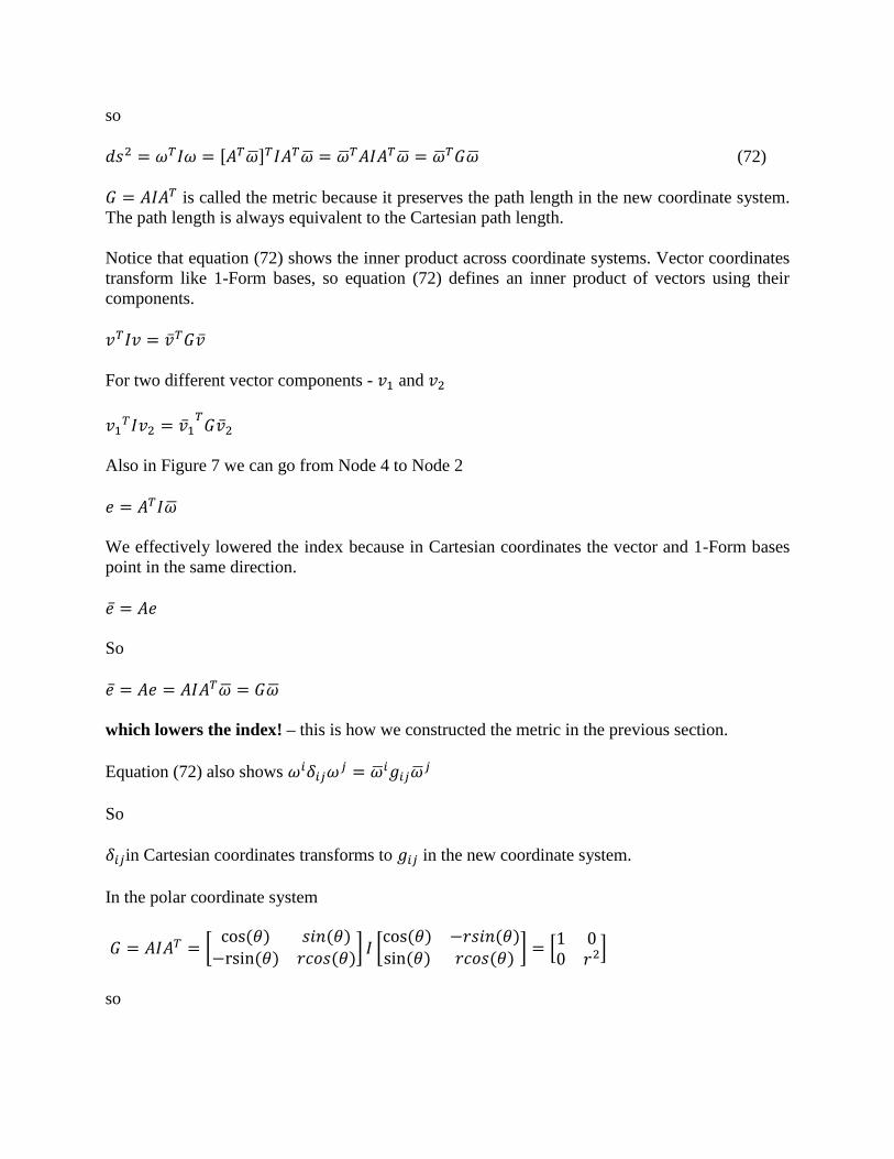
In the polar coordinate system

𝐺 = 𝐴𝐼𝐴𝑇 = [cos (𝜃) 𝑠𝑖𝑛(𝜃)

−rsin (𝜃) 𝑟𝑐𝑜𝑠(𝜃)] 𝐼 [

cos (𝜃) −𝑟𝑠𝑖𝑛(𝜃)sin (𝜃) 𝑟𝑐𝑜𝑠(𝜃)

] = [1 00 𝑟2]

so

𝑑𝑠2 = �̅�𝑇𝐺�̅� = [𝑑𝑟 𝑑𝜃] [1 00 𝑟2] [

𝑑𝑟𝑑𝜃

] = 𝑑𝑟2 + 𝑟2𝑑𝜃2

= [𝑐𝑜𝑠(𝜃)𝑑𝑥 + 𝑠𝑖𝑛(𝜃)𝑑𝑦]2 + 𝑟2 [−1

𝑟𝑠𝑖𝑛(𝜃)𝑑𝑥 +

1

𝑟𝑐𝑜𝑠(𝜃)𝑑𝑦]

2

= 𝑐𝑜𝑠2(𝜃)𝑑𝑥2 + 2𝑐𝑜𝑠(𝜃)𝑠𝑖𝑛(𝜃)𝑑𝑥𝑑𝑦 + 𝑠𝑖𝑛2(𝜃)𝑑𝑦2

+𝑠𝑖𝑛2(𝜃)𝑑𝑥2 − 2𝑠𝑖𝑛(𝜃)𝑐𝑜𝑠(𝜃)𝑑𝑥𝑑𝑦 + 𝑐𝑜𝑠2(𝜃)𝑑𝑦2

= [𝑐𝑜𝑠2(𝜃) + 𝑠𝑖𝑛2(𝜃)]𝑑𝑥2 + [𝑐𝑜𝑠2(𝜃) + 𝑠𝑖𝑛2(𝜃)]𝑑𝑦2 = 𝑑𝑥2 + 𝑑𝑦2

(73)

Equation (73) in Einstein notation is written as

𝑑𝑠2 = 𝑔𝑖𝑗𝑑𝑥𝑖𝑑𝑥𝑗 (74)

Where the units are 𝑚2

There is an inverse version of the path length.

Figure 8

Figure 8 shows a right triangle with height 𝑑ℎ perpendicular to side 𝑑𝑠.

There are two relations implied in Figure 8.

1.) Pythagorean Theorem

𝑑𝑠2 = 𝑑𝑥2 + 𝑑𝑦2

and

𝑑𝑥

𝑑𝑦

𝑑𝑠

𝑑ℎ

2.) Pythagorean Theorem for Reciprocals

[𝜕

𝜕ℎ]2

= [𝜕

𝜕𝑥]2

+ [𝜕

𝜕𝑦]2

1 (74)

where 𝑑ℎ is the height as shown in Figure 8.

For example if 𝑎 = 3, 𝑏 = 4, and 𝑐 = 5

Then Area =1

23 ∙ 4 = 6

1

25 ∙ ℎ = 6 → ℎ =

12

5

So

1

𝑎2+

1

𝑏2=

1

32+

1

42=

1

9+

1

16=

25

144= [

5

12]2

= [1

ℎ]

2

In vector form,

[𝜕

𝜕ℎ]2

= 𝑒𝑇𝑒 (75)

where 𝑒𝑇 = [𝜕

𝜕𝑥

𝜕

𝜕𝑦⋯]

From Figure 7,

𝑒 = 𝐵𝑇�̅� (76)

So

[𝜕

𝜕ℎ]2

= 𝑒𝑇𝐼𝑒 = [𝐵𝑇�̅�]𝑇𝐼[𝐵𝑇�̅�] = �̅�𝑇𝐵𝐼𝐵𝑇�̅� = �̅�𝑇𝐺−1�̅� (77)

We use 𝐺−1 because 𝐺𝐺−1 = 𝐴𝐴𝑇𝐵𝐵𝑇 = 𝐴𝐴𝑇[𝐴𝑇]−1𝐵𝑇 = 𝐴𝐵𝑇 = 𝐴𝐴−1 = 𝐼 (78)

Notice that equation (77) also defines an inner product. 1-Form components transform like bases

vectors

so

𝛼𝑇𝐼𝛼 = �̅�𝑇𝐺−1�̅�

define an inner product of 1-Form components.

1 http://www.cut-the-knot.org/pythagoras/PTForReciprocals.shtml

For two different 1-Form components - 𝛼1 and 𝛼2

𝛼1𝑇𝐼𝛼2 = �̅�1

𝑇𝐺−1�̅�2

Also in Figure 7 we can go from Node 3 to Node 1

𝜔 = 𝐼𝐵𝑇�̅�

We raised the index through the Cartesian Coordinate System

�̅� = 𝐵𝜔

So

�̅� = 𝐵𝐼𝐵𝑇�̅� = 𝐺−1�̅�

which raises the index! – this is how we constructed the inverse metric in the previous section.

Also

𝑒𝑖𝛿𝑖𝑗𝑒𝑗 = �̅�𝑖𝑔

𝑖𝑗�̅�𝑗

so

𝛿𝑖𝑗 in Cartesian Coordinates transforms to 𝑔𝑖𝑗 in the new system.

Equation (77) in Einstein notation is written as

[𝜕

𝜕ℎ]2

= 𝑔𝑖𝑗𝜕

𝜕𝑥𝑖

𝜕

𝜕𝑥𝑗

(79)

where the units 1

𝑚2

We can do a mixed upper and lower index scenario

[𝑑𝑥 + 𝑑𝑦] [𝜕

𝜕𝑥+

𝜕

𝜕𝑦] =

𝑑𝑥

𝑑𝑥+

𝑑𝑥

𝑑𝑦+

𝑑𝑦

𝑑𝑥+

𝑑𝑦

𝑑𝑦

(80)

But

𝑑𝑥

𝑑𝑦=

𝑑𝑦

𝑑𝑥= 0

So

(80) gives

𝑑𝑥

𝑑𝑥+

𝑑𝑦

𝑑𝑦= 2

In matrix form

𝜔𝑇𝑒 = [𝐴𝑇𝜔1]𝑇𝐵𝑇𝑒1 = 𝜔1𝑇𝐴𝐵𝑇𝑒1 = 𝜔1𝑇𝐴𝐴−1𝑒1 = 𝜔1𝑇𝑒1 = [𝑑𝑥 𝑑𝑦]

[

𝜕

𝜕𝑥𝜕

𝜕𝑦]

=𝑑𝑥

𝑑𝑥+

𝑑𝑦

𝑑𝑦= 2

The general case for N dimensions is �̅�𝑇�̅� = 𝑁

𝑔𝑖𝑗

= 𝑔𝑖𝑛𝑔𝑛𝑗 = 𝛿𝑖𝑗 matrix multiplication

𝑣𝑖 = 𝑔𝑖𝑗𝑣𝑗

𝛼𝑗 = 𝑔𝑖𝑗𝛼𝑖

𝜔𝑇𝐼𝑒 = �̅�𝑇𝐼�̅�

𝜔𝑗𝛿𝑖𝑗𝑒𝑖 = �̅�𝑗𝛿𝑖

𝑗�̅�𝑖

(81)

Equation (81) shows 𝛿𝑖𝑗 is invariant in any coordinate system

Equation (73) - 𝑑𝑠2 = �̅�𝑇𝐺�̅� - is an example of a tensor. A tensor is a mathematical construct

that allows the form of an equation to be the same in all coordinate systems.

𝑑𝑠2 = �̅�𝑇𝐺�̅� is invariant in any coordinate system. In Cartesian coordinates, �̅� = [𝑑𝑥𝑑𝑦

] and

𝐺 = 𝐼. In polar coordinates �̅� = [𝑑𝑟𝑑𝜃

] and 𝐺 = [1 00 𝑟2].

𝐺 is the metric tensor and 𝑑𝑠2 is the result of the metric tensor operating on �̅�𝑇 and �̅� which

creates a scalar. Tensors have different ranks. Tensors of rank 0 are scalars, tensors of rank 1 are

ordinary vectors. Tensors of rank 2 are matrices. The metric is a 2nd

rank tensor. Not all matrices

are 2nd

rank tensors. A 2nd

rank tensor has to allow the same form of an given equation in all

coordinate systems.

Figure 9 covers case where we don’t start from the Cartesian coordinate system – this is an

extension of Figure 7. The nodes on the right are from Figure 7

Figure 9

Figure 9 shows how 𝐺 transforms to a new system using equation (82) – start at Node 5 and

follow the red arrows as was shown previously.

�̅� = 𝐴𝐺𝐴𝑇 (82)

To convert it to Einstein notation take the following steps:

𝐴 =

[ 𝜕𝑥1

𝜕�̅�1

𝜕𝑥2

𝜕�̅�1⋯

𝜕𝑥1

𝜕�̅�2

𝜕𝑥2

𝜕�̅�2⋯

⋮ ⋮ ]

𝐺−1 𝐺

𝐵

𝐴𝑇

𝐴

𝐵𝑇 𝑒𝑖 , 𝛼𝑖

�̅�𝑖 , �̅�𝑖

�̅�𝑖, �̅�𝑖

𝜔𝑖, 𝑣𝑖

𝐵𝐺−1𝐵𝑇

𝐴𝐺𝐴𝑇

3

4 5

6

𝐴𝑇 =

[ 𝜕𝑥1

𝜕�̅�1

𝜕𝑥1

𝜕�̅�2⋯

𝜕𝑥2

𝜕�̅�1

𝜕𝑥2

𝜕�̅�2⋯

⋮ ⋮ ]

𝐴𝑇𝑚𝑛 =

𝜕𝑥𝑚

𝜕�̅�𝑛

(83)

[𝐺𝐴𝑇]𝑖𝑛 = 𝑔𝑖𝑗

𝜕𝑥𝑗

𝜕�̅�𝑛

(84)

𝐴𝑞𝑟 =𝜕𝑥𝑟

𝜕�̅�𝑞

(85)

𝐴𝐺𝐴𝑇 = 𝐴𝑞𝑖[𝐺𝐴𝑇]𝑖𝑛 =𝜕𝑥𝑖

𝜕�̅�𝑞𝑔𝑖𝑗

𝜕𝑥𝑗

𝜕�̅�𝑛= �̅�𝑞𝑛

This is the general transformation rule for the metric and any covariant 2nd

degree tensor.

Covariant 2nd

degree means that both indices are lower indices because they transform like the

vector basis functions.

Notice that the covariant kronecker delta transforms into the metric as we saw above.

[𝐼𝐴𝑇]𝑖𝑛 = 𝛿𝑖𝑗𝐴𝑇𝑗𝑛 = 𝛿𝑖𝑗

𝜕𝑥𝑗

𝜕�̅�𝑛

𝐺 = 𝐴𝐼𝐴𝑇 = 𝐴𝑚𝑖[𝐼𝐴𝑇]𝑖𝑛 =

𝜕𝑥𝑖

𝜕�̅�𝑚 𝛿𝑖𝑗

𝜕𝑥𝑗

𝜕�̅�𝑛= 𝑔𝑚𝑛

(86)

Figure 9 shows how 𝐺−1 transforms to a new system using equation (87). Start on Node 6 and

follow the green arrows.

�̅�−1 = 𝐵𝐺−1𝐵𝑇 (87)

To convert to Einstein notation, take the following steps:

𝐵 =

[ 𝜕�̅�1

𝜕𝑥1

𝜕�̅�1

𝜕𝑥2⋯

𝜕�̅�2

𝜕𝑥1

𝜕�̅�2

𝜕𝑥2⋯

⋮ ⋮ ]

𝐵𝑚𝑛 =𝜕�̅�𝑚

𝜕𝑥𝑛

(88)

𝐵𝑇𝑞𝑟 =

𝜕�̅�𝑟

𝜕𝑥𝑞

(89)

[𝐺−1𝐵𝑇]𝑖𝑟 = 𝑔𝑖𝑗𝜕�̅�𝑟

𝜕𝑥𝑗

(90)

𝐵𝐺−1𝐵𝑇 = 𝐵𝑚𝑖[𝐺−1𝐵𝑇]𝑖𝑟 =

𝜕�̅�𝑚

𝜕𝑥𝑖𝑔𝑖𝑗

𝜕�̅�𝑟

𝜕𝑥𝑗= �̅�𝑚𝑟

(91)

This is the general transformation rule for the metric and any contravariant 2nd

degree tensor –

both indices are in the numerator and transform like vector components.

Non Orthogonal Coordinate System Example

The last example is a non-orthogonal coordinate system. Figure 10 shows the Cartesian

coordinates with basis vectors 𝑒 = [𝑒1 𝑒2] and basis1-Forms 𝜔 = [𝜔1 𝜔2]. The non-

orthogonal coordinate system basis vectors are �̅� = [�̅�1 �̅�2].

Box 8

The Metric Adjusts in a Given Coordinate System

To Keep the Line Element Invariant

𝒅𝒔𝟐 = 𝝎𝑻𝑰𝝎 = �̅�𝑻𝑮�̅� [𝝏

𝝏𝒉]𝟐

= 𝒆𝑻𝑰𝒆 = �̅�𝑻𝑮−𝟏�̅�

The Metric Defines Inner Products

𝒗𝟏𝑻𝑰𝒗𝟐 = �̅�𝟏

𝑻𝑮 �̅�𝟐 and 𝜶𝟏

𝑻𝑰𝜶𝟐 = �̅�𝟏𝑻𝑮−𝟏 �̅�𝟐

The Metric Raises and Lowers Indices

�̅� = 𝑮�̅� and �̅� = 𝑮−𝟏�̅�

Metric Transformations

�̅� = 𝑨𝑮𝑨𝑻 and �̅�−𝟏 = 𝑩𝑮−𝟏𝑩𝑻

Figure 10

Equation (92) shows the Cartesian coordinates 𝑥 = [𝑥1 𝑥2] as functions of

the coordinates�̅� = [�̅�1 �̅�2].

𝑥1(�̅�1, �̅�2) = 𝑐𝑜𝑠 (𝜋

6) �̅�1 + 𝑐𝑜𝑠 (

𝜋

3) �̅�2 =

√3

2�̅�1 +

1

2�̅�2

𝑥2(�̅�1, �̅�2) = 𝑠𝑖𝑛 (𝜋

6) �̅�1 + 𝑠𝑖𝑛 (

𝜋

3) �̅�2 =

1

2�̅�1 +

√3

2�̅�2

(92)

Equation (93) shows the transformation matrix 𝐴 and equation (94) shows the vector bases

transformation equation.

𝐴 =𝜕𝑥𝑖

𝜕�̅�𝑗=

[ √3

2

1

21

2

√3

2 ]

(93)

𝜋

6

𝑒1

𝜋

6

𝜔1

𝑒2

𝜔2

�̅�1

�̅�2

�̅� = 𝐴𝑒

(94)

Equations (95) and (96) show the 𝐵 matrix and 1-Form bases equation.

𝐵 =𝜕�̅�𝑖

𝜕𝑥𝑗= (𝐴𝑇)−1 = [√3 −1

−1 √3]

(95)

�̅� = 𝐵𝜔

(96)

Figure 11 shows the Cartesian, �̅� , and �̅� coordinate systems.

Note:

�̅�1 and �̅�2 are length 1

�̅�1 and �̅�2 are length 2

�̅�1 ∙ �̅�2 = �̅�2 ∙ �̅�1 = 1(2)𝑐𝑜𝑠 (𝜋

2) = 0

�̅�1 ∙ �̅�1 = 2(1) cos (𝜋

3) =

2

2= 1

�̅�2 ∙ �̅�2 = 2(1) cos (𝜋

3) =

2

2= 1

So

�̅��̅�𝑇 = 𝑒𝜔𝑇 =𝑑�̅�𝑖

𝑑�̅�𝑗= 𝛿𝑗

𝑖= {

0 𝑖 ≠ 𝑗1 𝑖 = 𝑗

as we would expect!

Figure 11

Equation (98) transforms the vector coordinates 𝑣 = [32] to the �̅� system.

�̅� = 𝐵𝑣 = [33

2⁄ − 2

2√3 − 3] = [√3 −1

−1 √3] [

32] = 𝐵 [

32]

(98)

Equation (99) transforms the 1-Form coordinates 𝛼 = [32] to the �̅� system.

�̅�1

�̅�2

�̅�1

�̅�2

𝜋

6

𝜋

6

𝜋

6

𝜋

6

𝑒1

𝑒2

𝜋

6

𝜔1

𝜔2

�̅� = 𝐴𝛼 =

[ 3

32⁄ + 2

22√3 + 3

2 ]

=

[ √3

2

1

21

2

√3

2 ]

[32] = 𝐴 [

32]

(99)

In the Cartesian coordinate system, the inner product between 𝛼 and 𝑣 is shown in equation

(100),

𝛼𝑇𝑣 = [3 2] [32] = 9 + 4 = 13

(100)

Equation (101) shows the inner product between �̅� and �̅� in the �̅� coordinate system.

�̅�𝑇�̅� = [33

2⁄ + 2

2

2√3 + 3

2] [3

32⁄ − 2

2√3 − 3] =

[33

2⁄ + 2] [33

2⁄ − 2]

2+

=[2√3 + 3][2√3 − 3]

2=

27 − 4

2+

12 − 9

2=

23

2+

3

2= 13

(101)

Both Equations give the same answer as we expect.

The metric is given by equation (102)

𝐺 = 𝐴𝐼𝐴𝑇 = 𝑔𝑖𝑗 =

[ √3

2

1

21

2

√3

2 ]

[ √3

2

1

21

2

√3

2 ]

=

[ 3

4+

1

4

√3

4+

√3

4

√3

4+

√3

4

1

4+

3

4 ]

=

[ 1

√3

2

√3

21 ]

(102)

The path length is

𝑑𝑠2 = [𝑑�̅�1 𝑑�̅�2]

[ 1

√3

2

√3

21 ]

[𝑑�̅�1

𝑑�̅�2] = [𝑑�̅�1 𝑑�̅�2]

[ 𝑑�̅�1 +

√3

2𝑑�̅�2

√3

2𝑑�̅�1 + 𝑑�̅�2]

= 𝑑�̅�12 + 𝑑�̅�1

√3

2𝑑�̅�2 + 𝑑�̅�2

√3

2𝑑�̅�1 + 𝑑�̅�2

2 = 𝑑�̅�12 + √3𝑑�̅�1𝑑�̅�2 + 𝑑�̅�2

2

𝑑�̅�1 = √3𝑑𝑥1 − 𝑑𝑥2

and

𝑑�̅�2 = √3𝑑𝑥2 − 𝑑𝑥1

So

𝑑𝑠2 = 𝑑�̅�12 + √3𝑑�̅�1𝑑�̅�2 + 𝑑�̅�2

2 = [√3𝑑𝑥1 − 𝑑𝑥2]2

+ √3[√3𝑑𝑥1 − 𝑑𝑥2][√3𝑑𝑥2 − 𝑑𝑥1] +

[√3𝑑𝑥2 − 𝑑𝑥1]2

= 3𝑑𝑥12 − 2√3𝑑𝑥1𝑑𝑥2 + 𝑑𝑥2

= −3𝑑𝑥12 + 4√3𝑑𝑥1𝑑𝑥2 − 3𝑑𝑥2

2

= 𝑑𝑥12 − 2√3𝑑𝑥1𝑑𝑥2 + 3𝑑𝑥2

2

= 𝑑𝑥12 + 𝑑𝑥2

2

(103)

which is what we expect!