Curves

Hakan Bilen

University of Edinburgh

Computer Graphics

Fall 2017

Some slides are courtesy of Steve Marschner and Taku Komura

How to create a virtual world?

To compose scenes

We need to define objects

- Characters

- Terrains

- Objects (trees, furniture, buildings etc)

Geometric representations

• Meshes

• Triangle, quadrilateral,

polygon

• Implicit surfaces

• Blobs, metaballs

• Parametric surfaces / curves

• Polynomials

• Bezier curves, B-splines

Smoothness

Motivation

Many applications require smooth surfaces

Can produce smooth surfaces with less parameters

• Easier to design • Can efficiently preserve complex structures

[sce

ne

36

0.c

om

]

Original Spline

From draftsmanship to CG

• Control

• user specified control points

• analogy: ducks

• Smoothness

• smooth functions

• usually low order polynomials

• analogy: physical constraints, optimization

What is a curve?

A set of points that the pen traces over an interval of time

What is the dimensionality?

Implicit form: f x, y = 𝑥2 + 𝑦2 − 1 = 0

• Find the points that satisfy the equation

Parametric form: x, y = f t = 𝑐𝑜𝑠𝑡, 𝑠𝑖𝑛𝑡 , 𝑡 ∈ [0,2𝜋)

• Easier to draw

in this context

What is a spline curve?

𝑓 𝑡 is a

• parametric curve

• piecewise polynomial function that switches between different

functions for different t intervals

Example:

𝑓 𝑡 = ൞𝑡3, if 0 ≤ 𝑡 < 1

1 − 𝑡 − 1 3, if 1 ≤ 𝑡 < 20, otherwise

Defining spline curves

• Discontinuities at the integers [t=k]

• Each spline piece is defined over [k,k+1] (e.g. a cubic spline)

𝑓 𝑡 = 𝑎𝑡3 + 𝑏𝑡2 + 𝑐𝑡 + 𝑑

• Different coefficients for every interval

• Control of spline curves

• Interpolate

• Approximate

Today

• Spline segments

• Linear

• Quadratic

• Hermite

• Bezier

• Chaining splines

• Notation

• vectors bold and lowercase 𝒗

• points as column vector 𝒑 = 𝑝𝑥 𝑝𝑦

• matrices bold and uppercase 𝑴

Linear Segment

Spline segments

A line segment connecting point 𝒑𝒐 to 𝒑𝟏

Such that 𝑓 0 = 𝒑𝟎 and 𝑓 1 = 𝒑𝟏

𝑓𝑥 𝑡 = 1 − 𝑡 𝒙𝒐 + 𝑡𝒙𝟏

𝑓𝑦 𝑡 = 1 − 𝑡 𝒚𝒐 + 𝑡𝒚𝟏

Vector formulation

𝑓 𝑡 = 1 − 𝑡 𝒑𝒐 + 𝑡𝒑𝟏

Matrix formulation

𝑓 𝑡 = 𝑡 1? ?? ?

𝒑𝟎𝒑𝟏

𝑓 𝑡 = 𝑡 1−1 11 0

𝒑𝟎𝒑𝟏

𝒑𝟎

𝒑𝟏

1 − 𝑡

𝑡

1 − 𝑡 𝒑𝒐 + 𝑡𝒑𝟏

Matrix form of spline

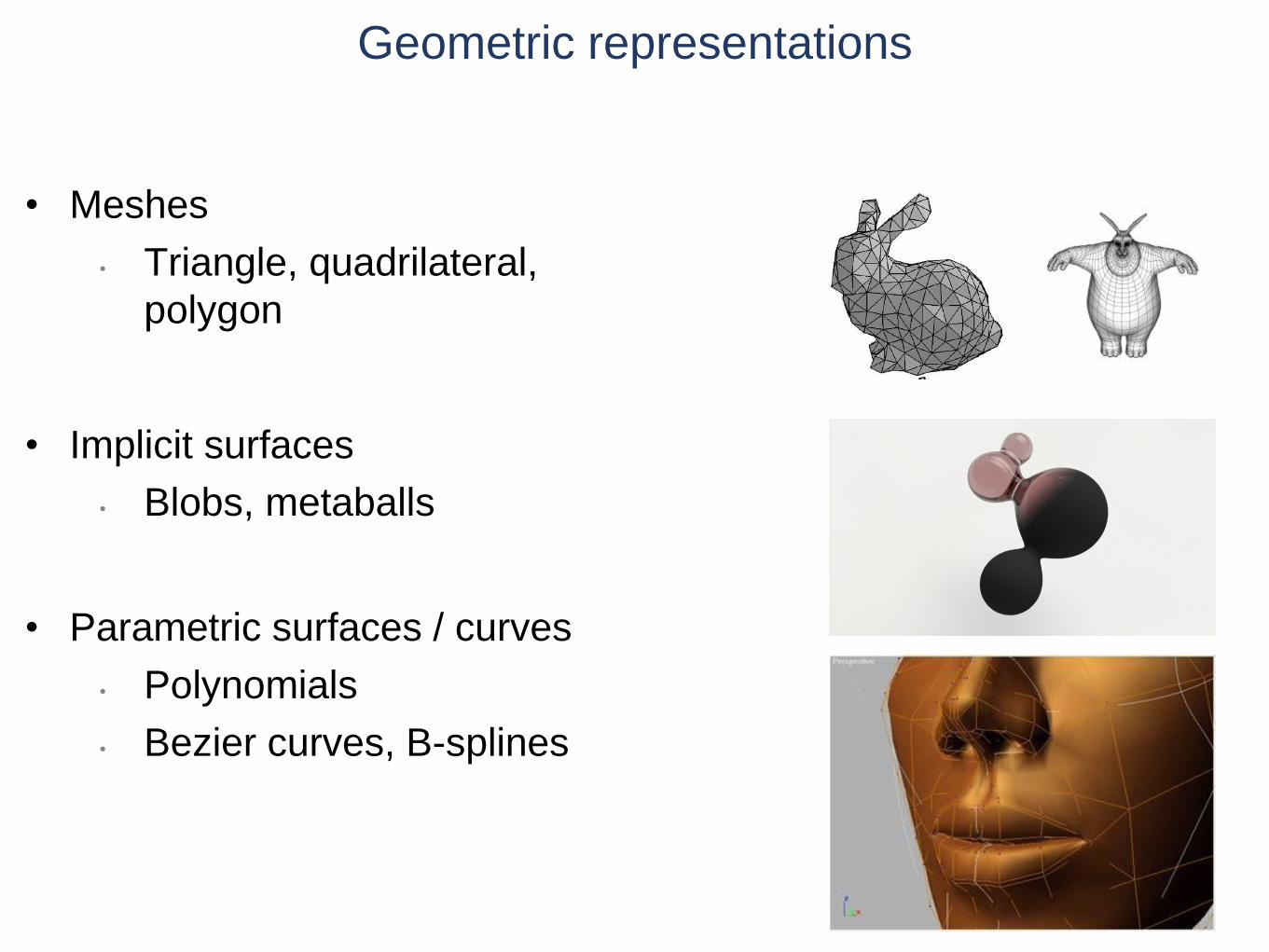
𝑓 𝑡 = 𝑡 1−1 11 0

𝒑𝟎𝒑𝟏

Blending functions 𝒃 𝑡 specify how to blend the values of the control point vector

𝒇 𝑡 = 𝒃𝟎 𝑡 𝒑𝟎 + 𝒃𝟏 𝑡 𝒑𝟏

𝒃𝟎 𝑡 = 1 − 𝑡

𝒃𝟏 𝑡 = 𝑡

𝒃𝟎 𝑡 𝒃𝟏 𝑡

Quadratic

Beyond line segment

A quadratic (𝒇 𝑡 = 𝑎0 + 𝑎1𝑡 + 𝑎2𝑡2) passes through 𝒑𝟎, 𝒑𝟏, 𝒑𝟐 s.t.

𝒑𝟎 = 𝑓 0 = 𝑎0 + 0 𝑎1 + 02 𝑎2

𝒑𝟏 = 𝑓 0.5 = 𝑎0 + 0.5 𝑎1+0.52 𝑎2

𝒑𝟐 = 𝑓 1 = 𝑎0 + 1 𝑎1 + 12 𝑎2

Points can be written in terms of constraint matrix 𝑪

𝒑𝟎𝒑𝟏𝒑𝟐

= 𝑪𝒂 ⇒

𝒑𝟎𝒑𝟏𝒑𝟐

=1 0 01 0.5 0.251 1 1

𝑎0𝑎1𝑎2

⇒

𝑎0𝑎1𝑎2

= 𝑪−𝟏𝒑𝟎𝒑𝟏𝒑𝟐

𝒇 𝑡 can be written in terms of basis matrix 𝑩 = 𝑪−𝟏 and points 𝒑

𝒇 𝑡 = 𝒕𝑩𝒑 = 𝒕𝑪−1𝒑 = 𝑡2 𝑡 12 −4 2−3 4 −11 0 0

𝒑𝟎𝒑𝟏𝒑𝟐

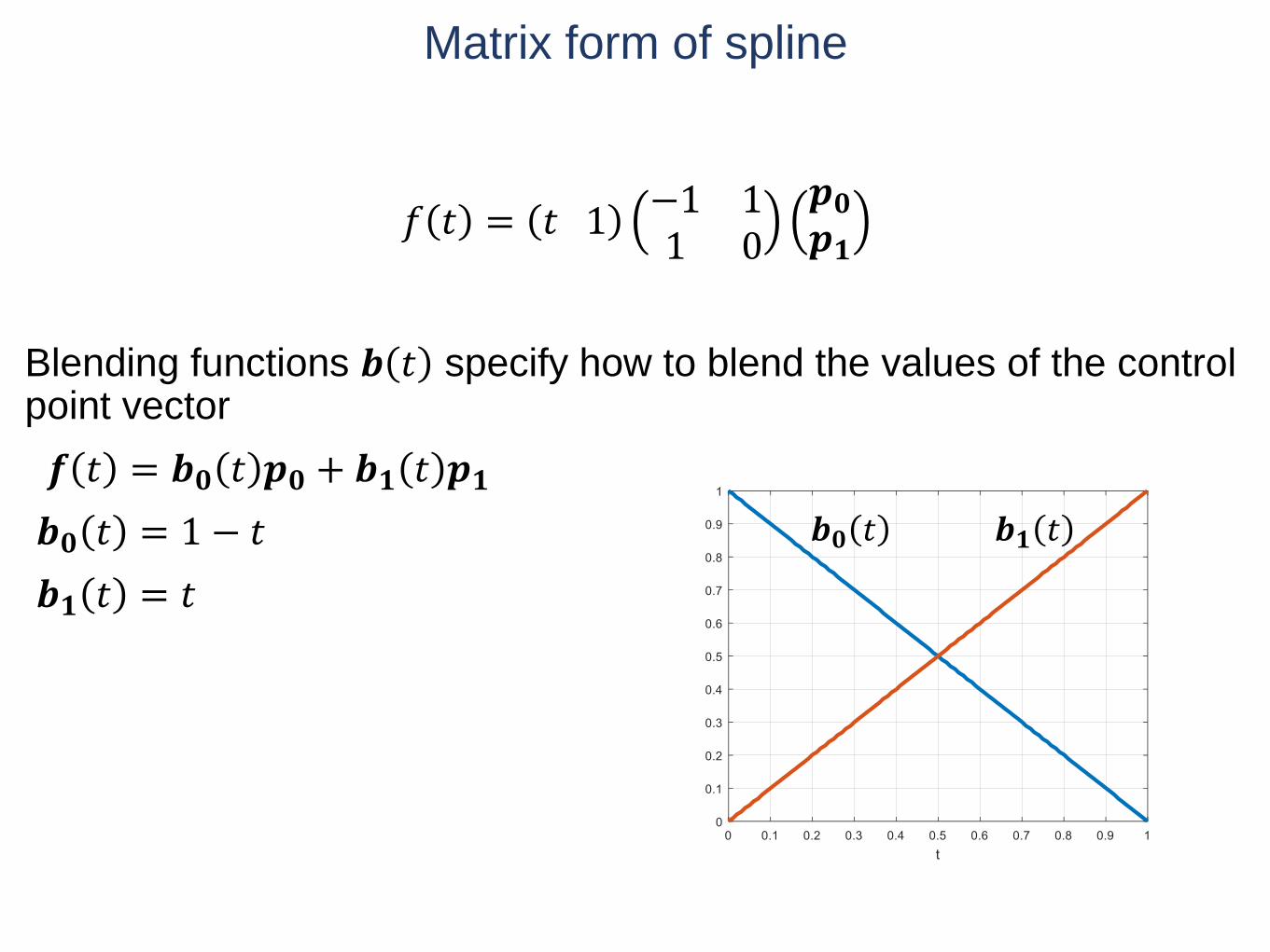
Blending functions

Matrix form of spline

𝒇 𝑡 = 𝑡2 𝑡 12 −4 2−3 4 −11 0 0

𝒑𝟎𝒑𝟏𝒑𝟐

Blending functions 𝒃 𝑡 specify how to blend the values of the control

point vector

𝒇 𝑡 = 𝒃𝟎 𝑡 𝒑𝟎 + 𝒃𝟏 𝑡 𝒑𝟏 + 𝒃𝟐 𝑡 𝒑𝟐

𝒃𝟎 𝑡 = 2𝑡2 − 3𝑡 + 1

𝒃𝟏 𝑡 = −4𝑡2 − 4𝑡

𝒃𝟐 𝑡 = 2𝑡2 − 1

Hermite spline

• Piecewise cubic (𝒇 𝑡 = 𝑎0 + 𝑎1𝑡 + 𝑎2𝑡2 + 𝑎3𝑡

3)

• Additional constraint on tangents (derivatives)

• 𝒇 𝑡 = 𝑎0 + 𝑎1𝑡 + 𝑎2𝑡2 + 𝑎3𝑡

3

• 𝒇′ 𝑡 = 𝑎1 + 2𝑎2𝑡 + 3𝑎3𝑡2

• 𝒑𝟎 = 𝑓 0 = 𝑎0• 𝒑𝟏 = 𝑓 1 = 𝑎0 + 𝑎1 + 𝑎2 + 𝑎3• 𝒗1 = 𝑓′(0) = 𝑎1• 𝒗2 = 𝑓′ 1 = 𝑎1 + 2𝑎2 + 3𝑎3

• Simpler matrix form

𝒇 𝑡 = 𝑡3 𝑡2 𝑡 1

2 −2 1 1−3 3 −2 −10 0 1 02 0 0 2

𝒑𝟎𝒑𝟏𝒗𝟏𝒗𝟐

𝒑𝟎

𝒑𝟏𝒗𝟎

𝒗𝟏

Hermite to Bézier

Specify tangents as points

• 𝑝0 = 𝑞0, 𝑝1 = 𝑞3, 𝑣0 = 3 𝑞1 − 𝑞0 , 𝑣1 = 3 𝑞3 − 𝑞2

•

𝒑𝟎𝒑𝟏𝒗𝟏𝒗𝟐

=

1 0 0 00 0 0 1−3 3 1 00 0 −3 3

𝒒𝟎𝒒𝟏𝒒𝟐𝒒𝟑

• Update Hermite eq. (from previous slide)

𝒇 𝑡 = 𝑡3 𝑡2 𝑡 1

2 −2 1 1−3 3 −2 −10 0 1 02 0 0 2

1 0 0 00 0 0 1−3 3 1 00 0 −3 3

𝒒𝟎𝒒𝟏𝒒𝟐𝒒𝟑

−𝒗𝟏

𝒒𝟏

𝒒𝟑

𝒒𝟐

𝒒𝟎

𝒗𝟏

𝒑𝟎 𝒑𝟏

𝒗𝟎

Bézier matrix

𝒇 𝑡 = 𝑡3 𝑡2 𝑡 1

−1 3 −3 13 −6 3 0−3 3 0 02 0 −6 6

𝒒𝟎𝒒𝟏𝒒𝟐𝒒𝟑

• 𝒇 𝑡 = σ𝑛=0𝑑 𝒃𝒏,𝟑𝒒𝒏

• Blending functions 𝒃 𝑡 has a special name in this case:

• Bernstein polynomials

𝑏𝑛,𝑘 =𝑛𝑘

𝑡𝑘 1 − 𝑡 𝑛−𝑘

and that defines Bézier curves for any degree

Bézier blending functions

• The functions sum to 1 at

any point along the curve.

• Endpoints have full weight

10/10/2008

q0 q3

q1 q2

de Casteljau algorithm

Another view to Bézier segments

Blend each linear spline with 𝛼 and 𝛽 = 1 − 𝛼

𝒑𝟎

𝒑𝟏

𝛼

𝛽

𝛼𝒑𝟎 + 𝛽𝒑𝟏

𝒑𝟎

𝒑𝟏

𝛼

𝛽

𝛼2𝒑𝟎 + 2𝛼𝛽𝒑𝟏 + 𝛽2𝒑𝟏

𝒑𝟐

𝛽

𝛼

Review

http://www.inf.ed.ac.uk/teaching/courses/cg/d3/hermite.html

http://www.inf.ed.ac.uk/teaching/courses/cg/d3/bezier.html

http://www.inf.ed.ac.uk/teaching/courses/cg/d3/Casteljau.html

Today

• Spline segments

• Linear

• Quadratic

• Hermite

• Bezier

• Chaining splines

• Continuity and local control

• Hermite curves

• Bezier curves

• Catmull-Rom curves

• B-splines

Putting segments together

• Limited degree of freedom with a single polynomial

• Will it be smooth enough?

Continuity

Measuring smoothness

Smoothness as degree of continuity

• zero-order (𝐶0): position match

• first-order (𝐶1): tangent match

• second-order (𝐶2): curvature match

• 𝐶𝑁 𝑣𝑠 𝐺𝑁

Putting segments together

• Limited degree of freedom with a single polynomial

• Will it be smooth enough?

• Local control

Local control

How many knots for m segments with 2 control points each?

Local control

?

Local control

• changing control point only affects a limited part of spline

– without this, splines are very difficult to use

• overshooting

• fixed computation

– many likely formulations lack this

• natural spline

• polynomial fits (matlab demo)

Piecewise linear

Putting segments together

Blending functions for a linear segment (0<t<1)

𝒇 𝑡 = 1 − 𝑡 𝒑𝟎 + 𝑡𝒑𝟏

𝒑𝟎

𝒑𝟏

𝒇 𝑡

𝒑𝟎 𝒑𝟏

Piecewise linear

Putting segments together

𝒇𝟎 𝑡 = 1 − 𝑡 𝒑𝟎 + 𝑡𝒑𝟏 (0 < 𝑡 < 1)

𝒇𝟏 𝑡 = ? 𝒑𝟏 + ? 𝒑𝟐 (1 < 𝑡 < 2)

𝒇𝟏 𝑡 = 2 − 𝑡 𝒑𝟏 + 𝑡 − 1 𝒑𝟐 (1 < 𝑡 < 2)

𝒑𝟎

𝒑𝟏

𝒇𝟎 𝑡

𝒑𝟐

𝒇𝟏 𝑡

𝒑𝟎 𝒑𝟏 𝒑𝟏 𝒑𝟐

Putting segments together

How can we chain these segments to a longer curve?

• Use first segment between t=0 to t=1

• Use second segment between t=1 to t=2

𝑓 𝑡 = 𝑓𝑖 𝑡 − 𝑖 for 𝑖 ≤ 𝑡 ≤ 𝑖 + 1

• Shift blending functions

𝑓0 𝑡 = 𝑏0 𝑡 𝒑𝟎 + 𝑏1 𝑡 𝒑𝟏

𝑓1 𝑡 = 𝑏0 𝑡 − 1 𝒑𝟏 + 𝑏1 𝑡 − 1 𝒑𝟐

• Match derivatives at end points to avoid discontinuity

Hermite basis

Slide credit: S. Marschner

• How many segments for n control points?

(n-2)/2

• Continuity?

𝐶1

Can we add blending functions as in Hermite?

• If 𝑝3 − 𝑝2 is collinear with 𝑝4 − 𝑝3 , it is

𝐺1 continuous

• 𝑝3 − 𝑝2 = 𝑘(𝑝4 − 𝑝3), 𝑘 > 0

• If tangents match, it is 𝐶1 continuous

• 𝑝3 − 𝑝2 = 𝑘(𝑝4 − 𝑝3), k = 1

Chaining Bézier Splines

𝒑𝟏

𝒑𝟑

𝒑𝟐

𝒑𝟎

Chaining segments

• Hermite curves are convenient because they can be made long

easily

• Bézier curves are convenient because their controls are all points

– but it is fussy to maintain continuity constraints

– and they interpolate every 3rd point, which is a little odd

• We derived Bézier from Hermite by defining tangents from control

points

– a similar construction leads to the interpolating Catmull-Rom

spline

Catmull-Rom

Would like to define tangents automatically

– use adjacent control points

𝒒𝟏

𝒒𝟎 𝒒𝟑

𝒒𝟐

Hermite to Catmull-Rom

• 𝑝0 = 𝑓 0

• 𝑝1 = 𝑓 1

• 𝑣1 = 𝑓′(0)

• 𝑣2 = 𝑓′ 1

• 𝒇 𝑡 =

𝑡3 𝑡2 𝑡 1

2 −2 1 1−3 3 −2 −10 0 1 02 0 0 2

𝒑𝟎𝒑𝟏𝒗𝟎𝒗𝟏

• 𝑝0 = 𝑞1

• 𝑝1 = 𝑞2

• 𝑣0 =1

2(𝑞2 − 𝑞0)

• 𝑣1 =1

2(𝑞3 − 𝑞1)

𝒇 𝑡 = 𝑡3 𝑡2 𝑡 1

2 −2 1 1−3 3 −2 −10 0 1 02 0 0 2

0 1 0 00 0 1 0

−0.5 0 0.5 00 −0.5 0 0.5

𝒒𝟎𝒒𝟏𝒒𝟐𝒒𝟑

Catmull-Rom

• Interpolating curve

• Like Bézier, equivalent to Hermite

• Continuity ?

• Local control ?

• Add tension

• 𝑝0 = 𝑞1

• 𝑝1 = 𝑞2

• 𝑣0 =1

2(1 − 𝑡)(𝑞2 − 𝑞0)

• 𝑣1 =1

2(1 − 𝑡)(𝑞3 − 𝑞1)

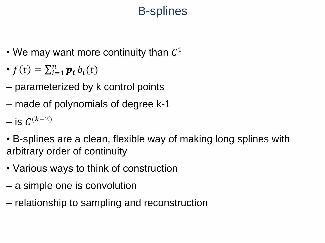
B-splines

• We may want more continuity than 𝐶1

• 𝑓 𝑡 = σ𝑖=1𝑛 𝒑𝒊 𝑏𝑖(𝑡)

– parameterized by k control points

– made of polynomials of degree k-1

– is 𝐶(𝑘−2)

• B-splines are a clean, flexible way of making long splines with

arbitrary order of continuity

• Various ways to think of construction

– a simple one is convolution

– relationship to sampling and reconstruction

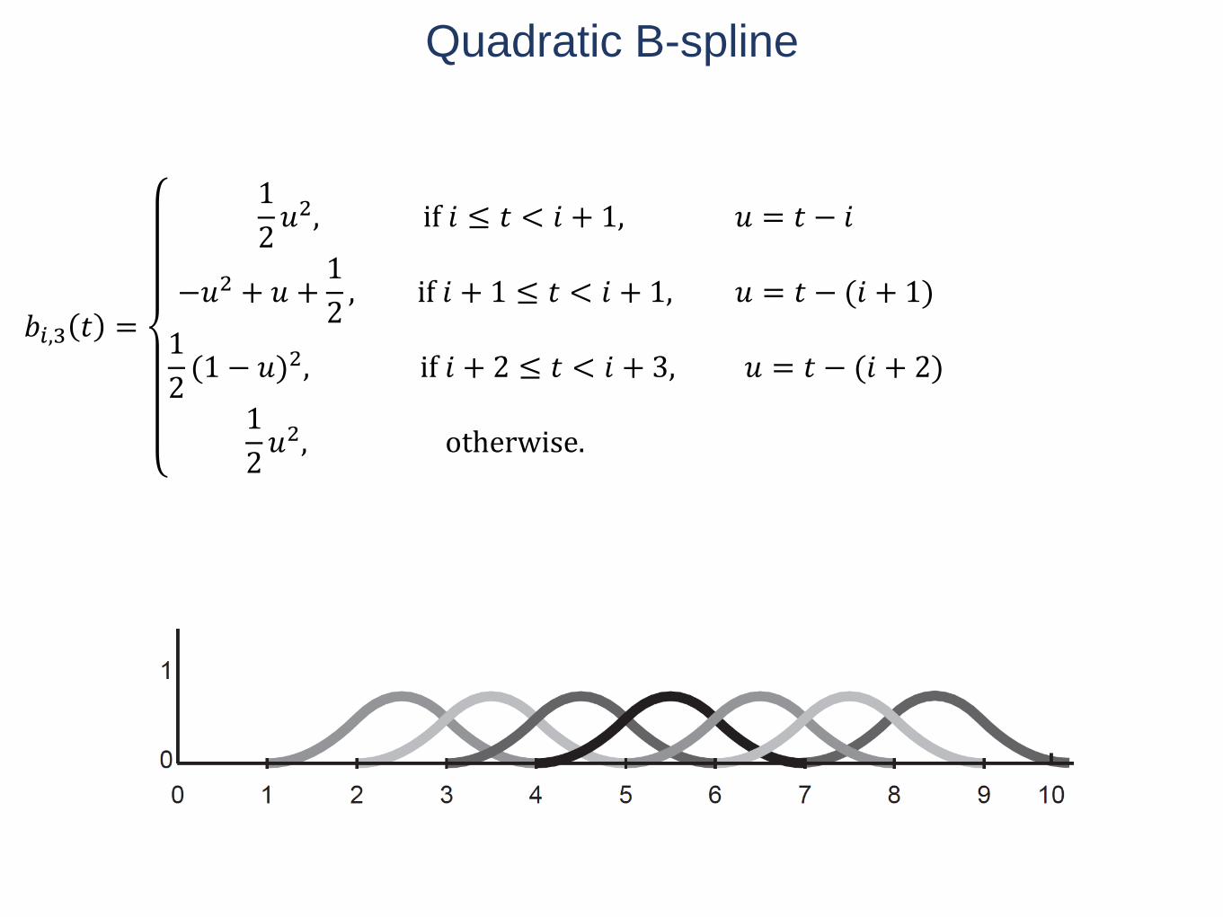
Quadratic B-spline

𝑏𝑖,3 𝑡 =

1

2𝑢2, if 𝑖 ≤ 𝑡 < 𝑖 + 1, 𝑢 = 𝑡 − 𝑖

−𝑢2 + 𝑢 +1

2, if 𝑖 + 1 ≤ 𝑡 < 𝑖 + 1, 𝑢 = 𝑡 − (𝑖 + 1)

1

2(1 − 𝑢)2, if 𝑖 + 2 ≤ 𝑡 < 𝑖 + 3, 𝑢 = 𝑡 − (𝑖 + 2)

1

2𝑢2, otherwise.

Smoothing effect

B-Spline

Summary

• Spline segments

• Linear

• Quadratic

• Hermite

• Bezier

• Chaining splines

• Catmull Rom curve and B-splines

• Suggested reading: B1 Chapter 15