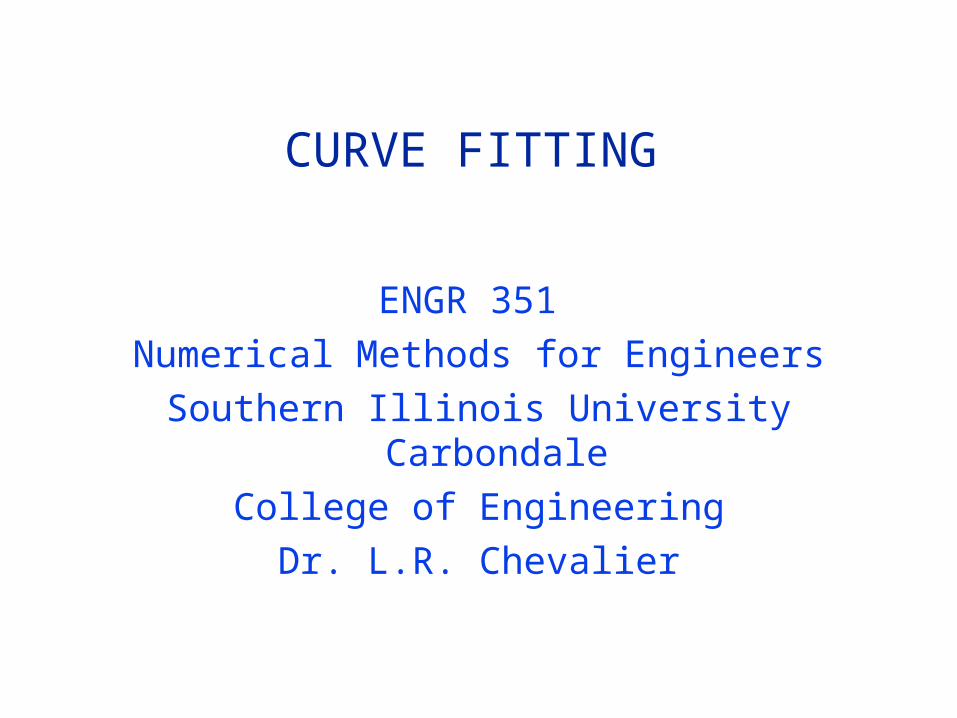
CURVE FITTING

ENGR 351 Numerical Methods for Engineers

Southern Illinois University Carbondale

College of EngineeringDr. L.R. Chevalier

Copyright © 2000 by Lizette R. Chevalier

Permission is granted to students at Southern Illinois University at Carbondaleto make one copy of this material for use in the class ENGR 351, NumericalMethods for Engineers. No other permission is granted.

All other rights are reserved. No part of this publication may be reproduced, stored in a retrieval system, or transmitted, in any form or by any means,electronic, mechanical, photocopying, recording, or otherwise, withoutthe prior written permission of the copyright owner.

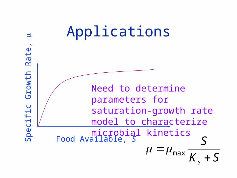
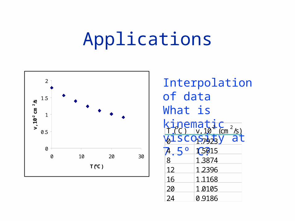
Applications

Food Available, S

Spe

cifi

c G

row

th R

ate,

Need to determine parameters for saturation-growth rate model to characterize microbial kinetics

SKS

s max

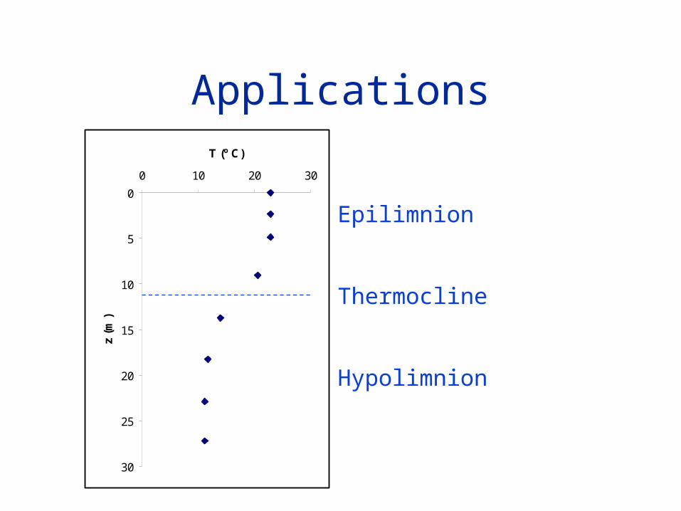
Applications

0

5

10

15

20

25

30

0 10 20 30

T (o C)

z (m

)

Epilimnion

Thermocline

Hypolimnion

0

0.5

1

1.5

2

0 10 20 30

T(oC)

v, 1

0-2 c

m2/s

Applications

Interpolation of dataWhat is kinematic viscosity at 7.5º C?

T (oC) v, 10-2 (cm2/s)

0 1.79234 1.56158 1.387412 1.239616 1.116820 1.010524 0.9186

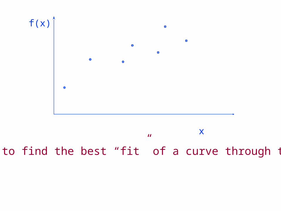
f(x)

x

We want to find the best “fit” of a curve through the data.

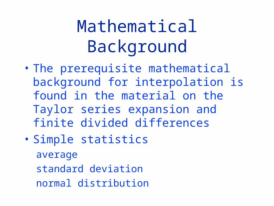
Mathematical Background

• The prerequisite mathematical background for interpolation is found in the material on the Taylor series expansion and finite divided differences

• Simple statisticsaverage

standard deviation

normal distribution

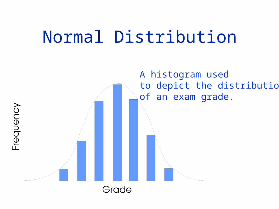
Normal Distribution

A histogram usedto depict the distributionsof an exam grade.

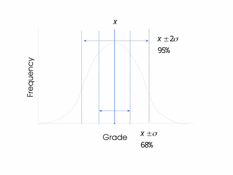
x

x 2

95%

x 68%

Material to be Covered in Curve Fitting

• Linear RegressionPolynomial Regression

Multiple Regression

General linear least squares

Nonlinear regression

• InterpolationNewton’s Polynomial

Lagrange polynomial

Coefficients of polynomials

Specific Study Objectives

• Understand the fundamental difference between regression and interpolation and realize why confusing the two could lead to serious problems

• Understand the derivation of linear least squares regression and be able to assess the reliability of the fit using graphical and quantitative assessments.

Specific Study Objectives

• Know how to linearize data by transformation• Understand situations where polynomial, multiple

and nonlinear regression are appropriate• Understand the general matrix formulation of

linear least squares• Understand that there is one and only one

polynomial of degree n or less that passes exactly through n+1 points

Specific Study Objectives

• Realize that more accurate results are obtained if data used for interpolation is centered around and close to the unknown point

• Recognize the liabilities and risks associated with extrapolation

• Understand why spline functions have utility for data with local areas of abrupt change

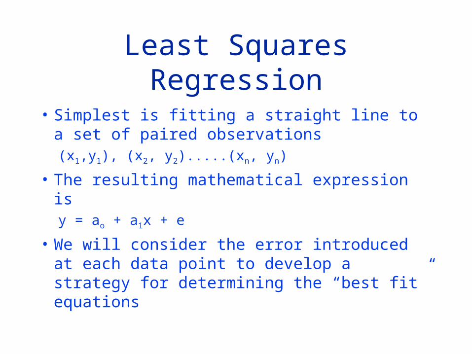
Least Squares Regression

• Simplest is fitting a straight line to a set of paired observations(x1,y1), (x2, y2).....(xn, yn)

• The resulting mathematical expression isy = ao + a1x + e

• We will consider the error introduced at each data point to develop a strategy for determining the “best fit” equations

S e y a a xri

n

i o ii

n

i

2

11

1

2

f(x)

x

y a a xi o i 1

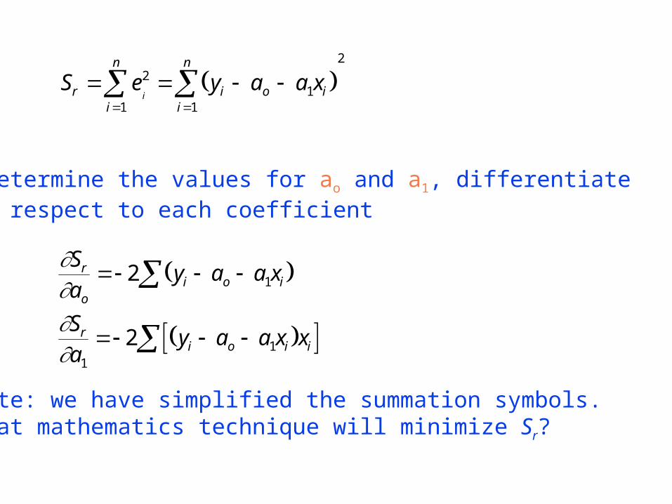
S e y a a xri

n

i o ii

n

i

2

11

1

2

To determine the values for ao and a1, differentiatewith respect to each coefficient

S

ay a a x

S

ay a a x x

r

oi o i

ri o i i

2

2

1

11

Note: we have simplified the summation symbols.What mathematics technique will minimize Sr?

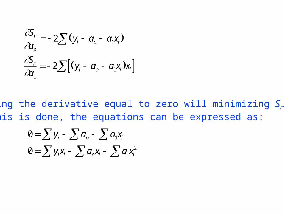
S

ay a a x

S

ay a a x x

r

oi o i

ri o i i

2

2

1

11

Setting the derivative equal to zero will minimizing Sr.If this is done, the equations can be expressed as:

0

0

1

12

y a a x

y x a x a x

i o i

i i o i i

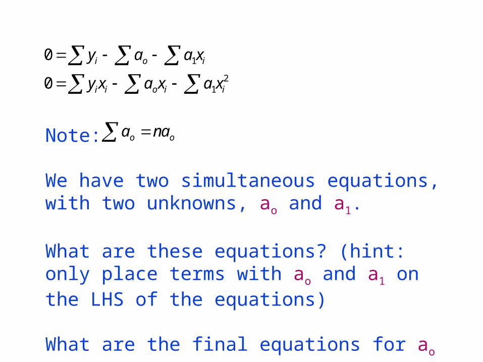
0

0

1

12

y a a x

y x a x a x

i o i

i i o i i

Note:

We have two simultaneous equations, with two unknowns, ao and a1.

What are these equations? (hint: only place terms with ao and a1 on the LHS of the equations)

What are the final equations for ao and a1?

a nao o

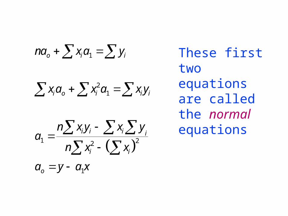
na x a y

x a x a x y

an x y x y

n x x

a y a x

o i i

i o i i i

i i i i

i i

o

1

21

1 2 2

1

These first twoequations are calledthe normal equations

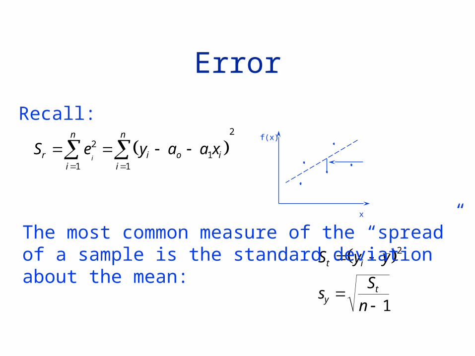
Error

S e y a a xri

n

i o ii

n

i

2

11

1

2

Recall:f(x)

x

S y y

sS

n

t i

yt

2

1

The most common measure of the “spread” of a sample is the standard deviation about the mean:

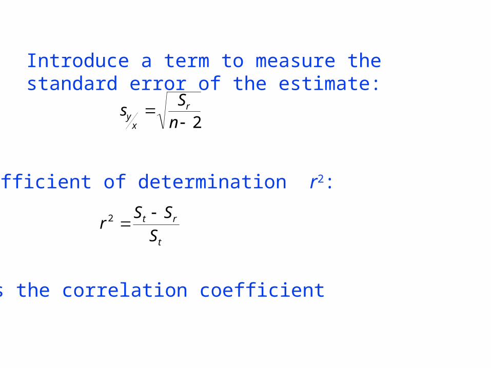
Introduce a term to measure the standard error of the estimate:

sS

nyx

r 2

Coefficient of determination r2:

rS S

St r

t

2

r is the correlation coefficient

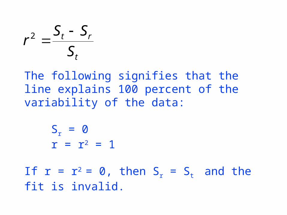
rS S

St r

t

2

The following signifies that the line explains 100 percent of the variability of the data:

Sr = 0 r = r2 = 1

If r = r2 = 0, then Sr = St and the fit is invalid.

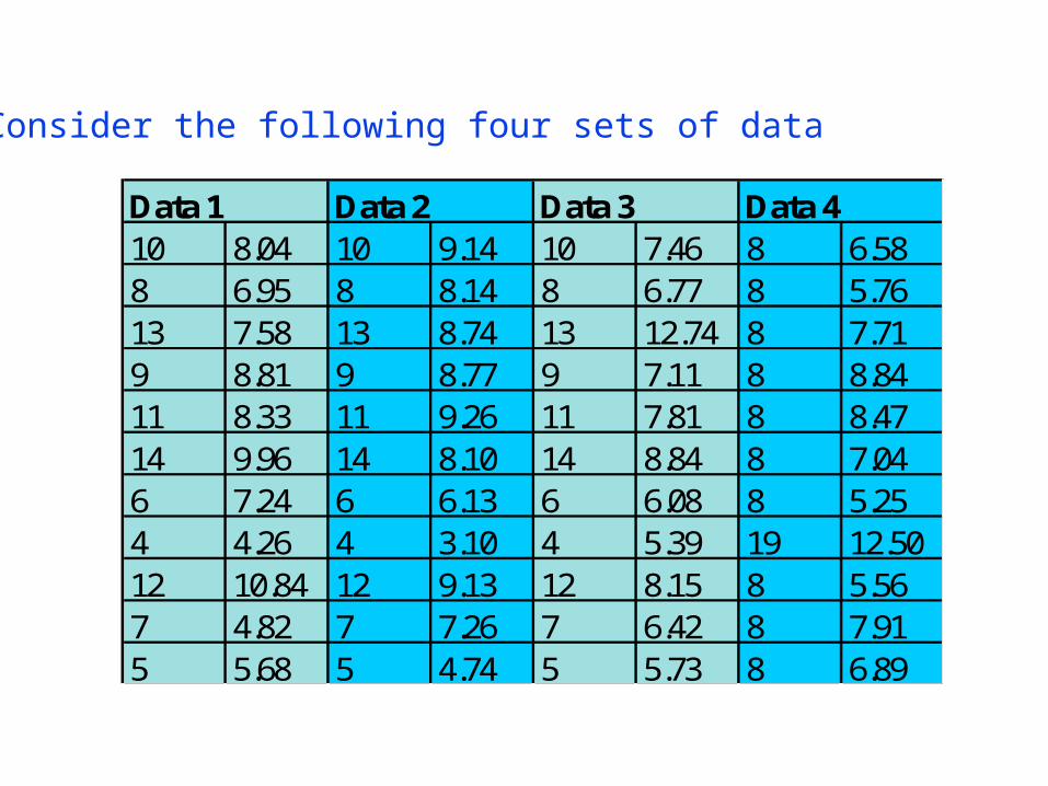
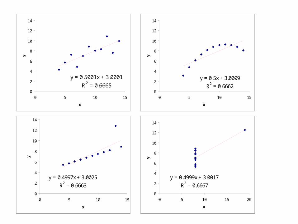
Data 1 Data 2 Data 3 Data 410 8.04 10 9.14 10 7.46 8 6.588 6.95 8 8.14 8 6.77 8 5.7613 7.58 13 8.74 13 12.74 8 7.719 8.81 9 8.77 9 7.11 8 8.8411 8.33 11 9.26 11 7.81 8 8.4714 9.96 14 8.10 14 8.84 8 7.046 7.24 6 6.13 6 6.08 8 5.254 4.26 4 3.10 4 5.39 19 12.5012 10.84 12 9.13 12 8.15 8 5.567 4.82 7 7.26 7 6.42 8 7.915 5.68 5 4.74 5 5.73 8 6.89

Consider the following four sets of data

y = 0.5001x + 3.0001

R2 = 0.66650

2

4

6

8

10

12

14

0 5 10 15

x

y

y = 0.5x + 3.0009

R2 = 0.66620

2

4

6

8

10

12

14

0 5 10 15

x

y

y = 0.4999x + 3.0017

R2 = 0.6667

0

2

4

6

8

10

12

14

0 5 10 15 20

x

y

y = 0.4997x + 3.0025

R2 = 0.6663

0

2

4

6

8

10

12

14

0 5 10 15

x

y

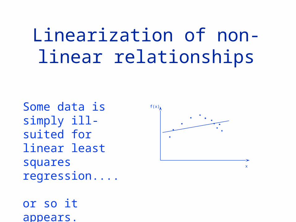
Linearization of non-linear relationships

Some data is simply ill-suited for linear least squares regression....

or so it appears.

f(x)

x

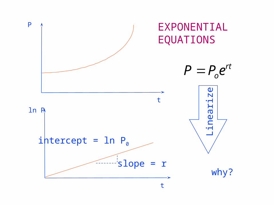
P

t

ln P

t

slope = r

intercept = ln P0

P P eort

Lin

eari

ze

why?

EXPONENTIALEQUATIONS

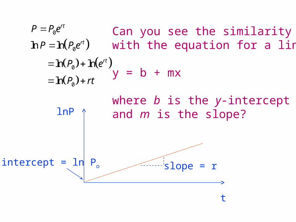
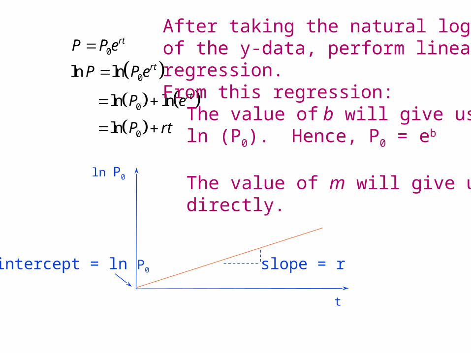
P P e

P P e

P e

P rt

rt

rt

rt

0

0

0

0

ln ln

ln ln

ln

slope = rintercept = ln Po

Can you see the similaritywith the equation for a line:

y = b + mx

where b is the y-intercept and m is the slope?lnP

t

P P e

P P e

P e

P rt

rt

rt

rt

0

0

0

0

ln ln

ln ln

ln

ln P0

t

slope = rintercept = ln P0

After taking the natural logof the y-data, perform linearregression.From this regression:

The value of b will give usln (P0). Hence, P0 = eb

The value of m will give us rdirectly.

POWER EQUATIONS

log Q

log H

Q

H

acHQ

Here we linearizethe equation bytaking the log ofH and Q data.What is the resultingintercept and slope?

(Flow over a weir)

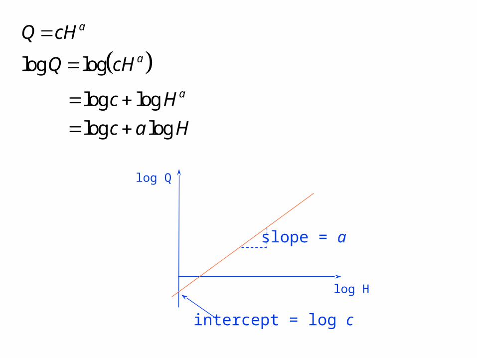
Q cH

Q cH

c H

c a H

a

a

a

log log

log log

log log

log Q

log H

slope = a

intercept = log c

So how do we getc and a fromperforming regressionon the log H vs log Qdata?From : y = mx + b

b = log c

c = 10b

m = a

log Q

log H

slope = a

intercept = log c

Q cH

Q cH

c H

c a H

a

a

a

log log

log log

log log

S1/

1/ S

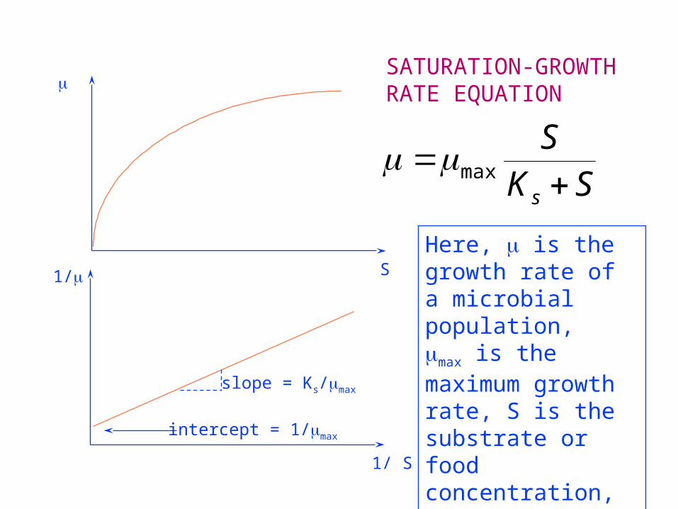
SATURATION-GROWTHRATE EQUATION

SKS

s max

slope = Ks/max

intercept = 1/max

Here, is the growth rate of a microbial population,max is the maximum growth rate, S is the substrate or food concentration, Ks is the substrate concentration at a value of = max/2

General Comments of Linear Regression

• You should be cognizant of the fact that there are theoretical aspects of regression that are of practical importance but are beyond the scope of this book

• Statistical assumptions are inherent in the linear least squares procedure

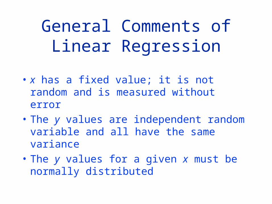
General Comments of Linear Regression

• x has a fixed value; it is not random and is measured without error

• The y values are independent random variable and all have the same variance

• The y values for a given x must be normally distributed

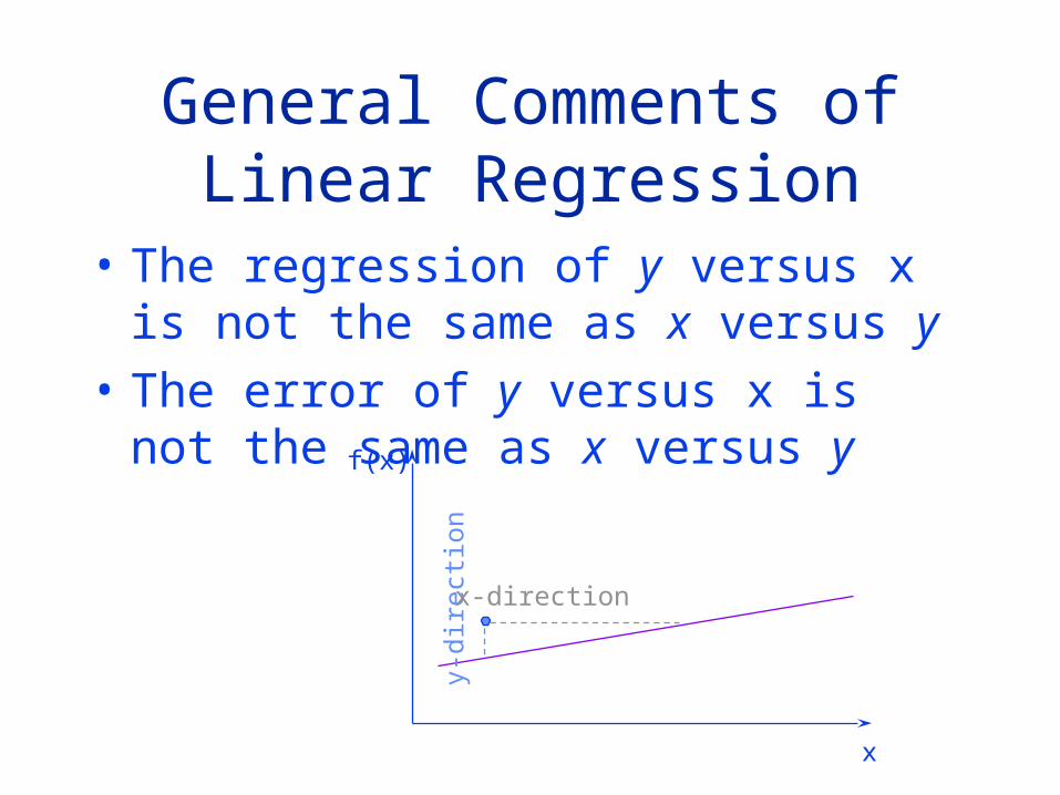
General Comments of Linear Regression

• The regression of y versus x is not the same as x versus y

• The error of y versus x is not the same as x versus y f(x)

x

y-di

rect

ion

x-direction

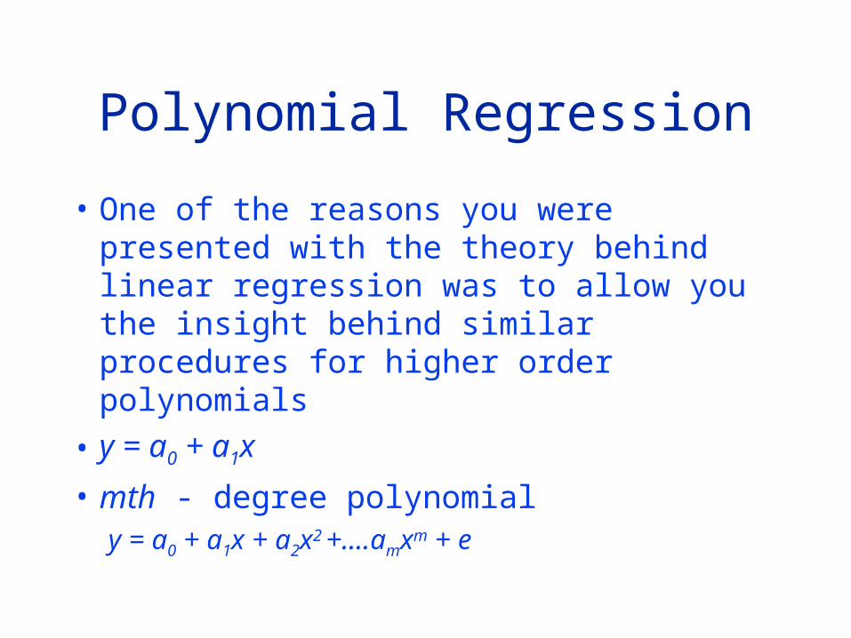
Polynomial Regression

• One of the reasons you were presented with the theory behind linear regression was to allow you the insight behind similar procedures for higher order polynomials

• y = a0 + a1x

• mth - degree polynomialy = a0 + a1x + a2x2 +....amxm + e

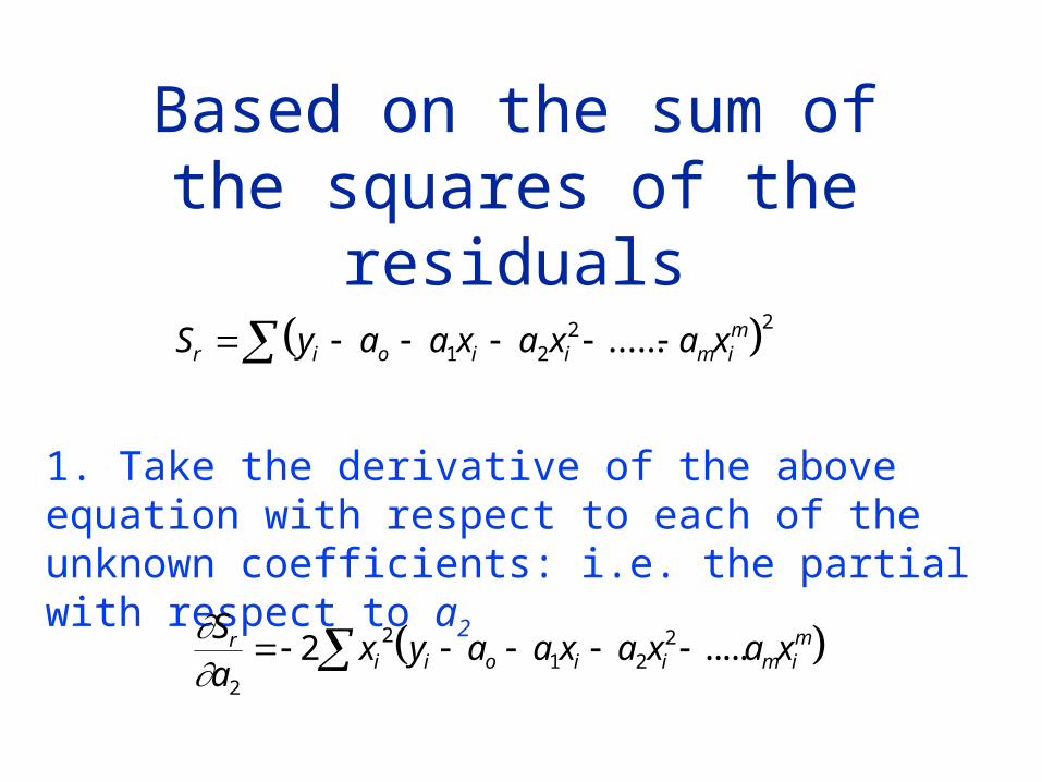
Based on the sum of the squares of the residuals

S y a a x a x a xr i o i i m im 1 2

2 2......

1. Take the derivative of the above equation with respect to each of the unknown coefficients: i.e. the partial with respect to a2

S

ax y a a x a x a xr

i i o i i m im

2

21 2

22 .....

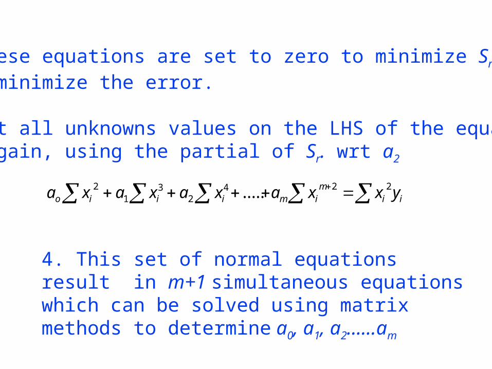
2. These equations are set to zero to minimize Sr., i.e. minimize the error.

3. Set all unknowns values on the LHS of the equation. Again, using the partial of Sr. wrt a2

a x a x a x a x x yo i i i m im

i i2

13

24 2 2 .....

4. This set of normal equations result in m+1 simultaneous equations which can be solved using matrix methods to determine a0, a1, a2......am

Multiple Linear Regression

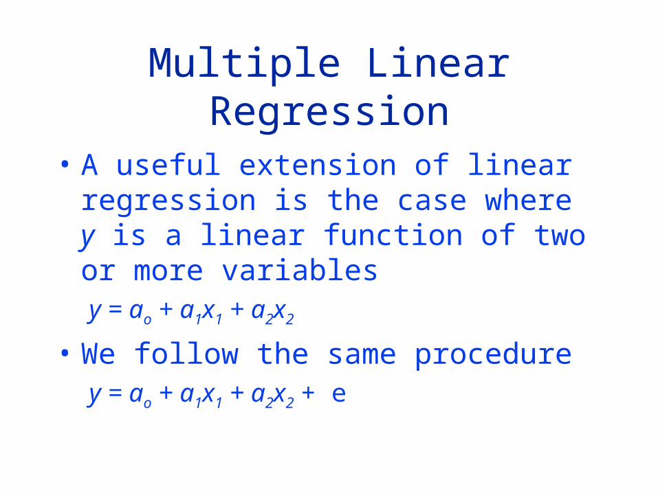
• A useful extension of linear regression is the case where y is a linear function of two or more variablesy = ao + a1x1 + a2x2

• We follow the same procedurey = ao + a1x1 + a2x2 + e

Multiple Linear Regression

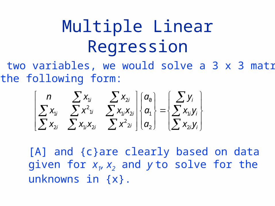
For two variables, we would solve a 3 x 3 matrixin the following form:

n x x

x x x x

x x x x

a

a

a

y

x y

x y

i i

i i i i

i i i i

i

i i

i i

1 2

12

1 1 2

2 1 22

2

0

1

2

1

2

[A] and {c}are clearly based on data given for x1, x2 and y to solve for the unknowns in {x}.

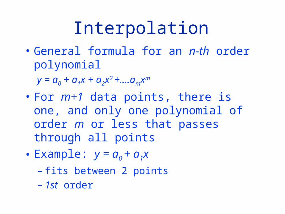
Interpolation• General formula for an n-th order

polynomialy = a0 + a1x + a2x2 +....amxm

• For m+1 data points, there is one, and only one polynomial of order m or less that passes through all points

• Example: y = a0 + a1x

– fits between 2 points– 1st order

Interpolation

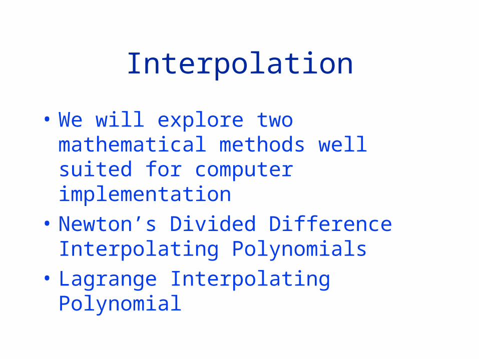
• We will explore two mathematical methods well suited for computer implementation

• Newton’s Divided Difference Interpolating Polynomials

• Lagrange Interpolating Polynomial

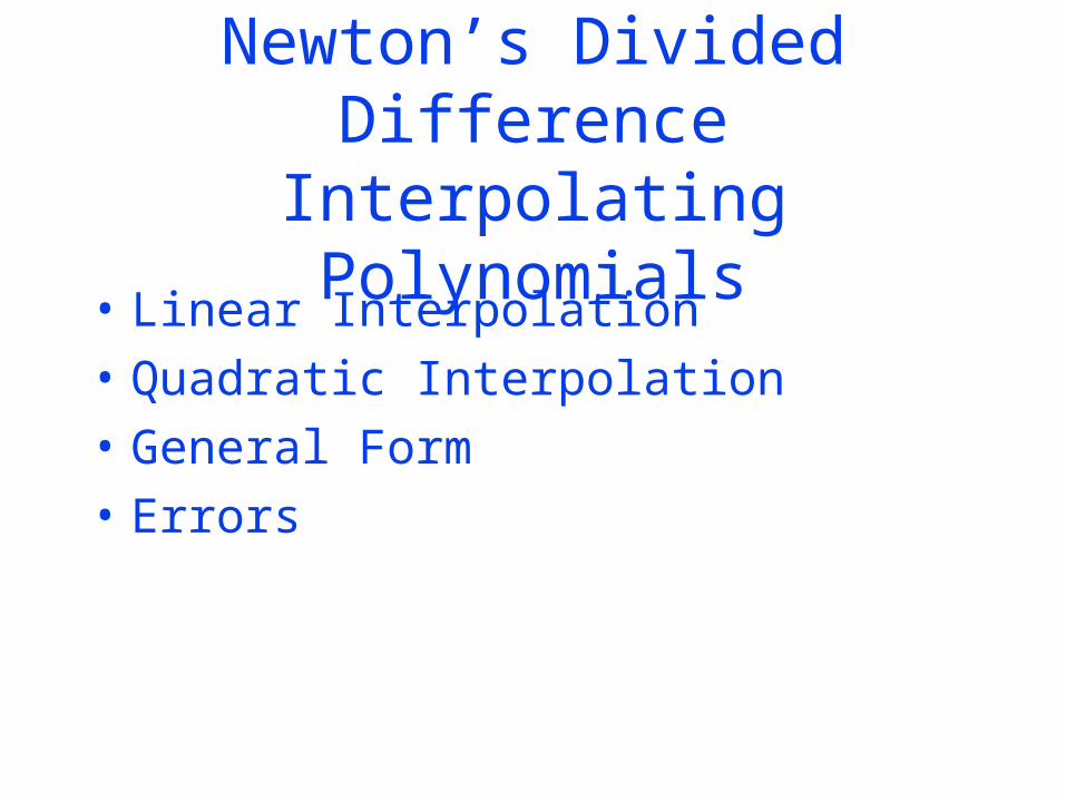
Newton’s Divided Difference Interpolating Polynomials

• Linear Interpolation

• Quadratic Interpolation

• General Form

• Errors

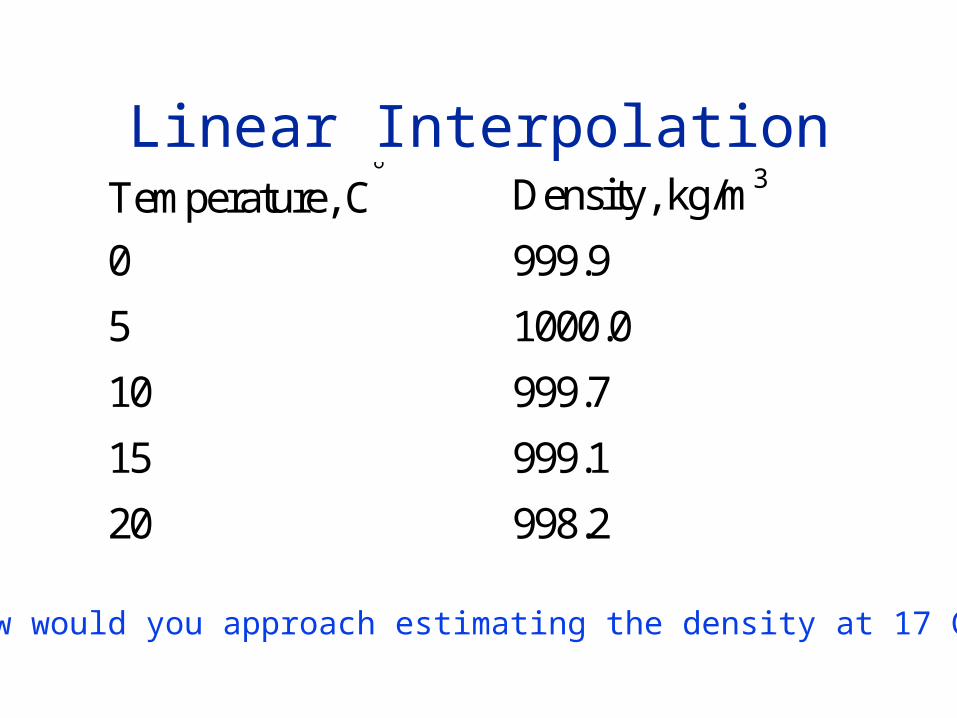
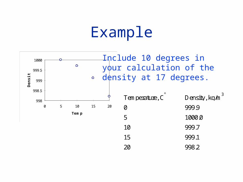
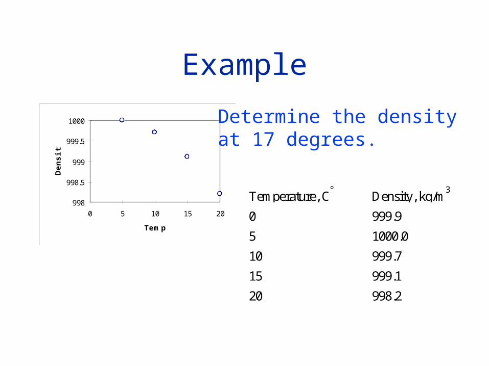
Linear InterpolationTemperature, C Density, kg/m3

0 999.9

5 1000.0

10 999.7

15 999.1

20 998.2

How would you approach estimating the density at 17 C?

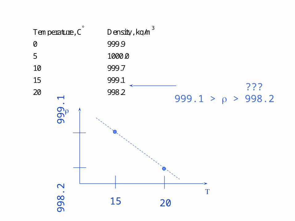
Temperature, C Density, kg/m3

0 999.9

5 1000.0

10 999.7

15 999.1

20 998.2 ???999.1 > > 998.2

15 20

998.

2

999.

1

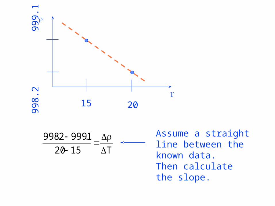
Assume a straight line between the known data.Then calculate the slope.T1520

1.9992.998

15 20

998.

2

999.

1

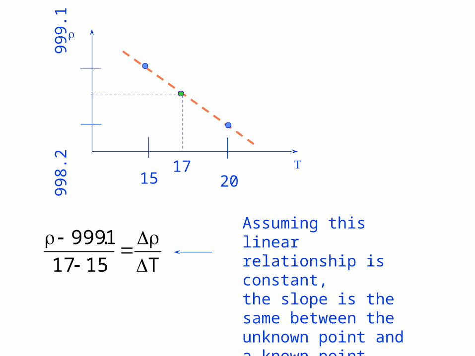
Assuming this linear relationship is constant,the slope is the same between the unknown point and a known point.

T1517

1.999

15 20

998.

2

999.

1

17

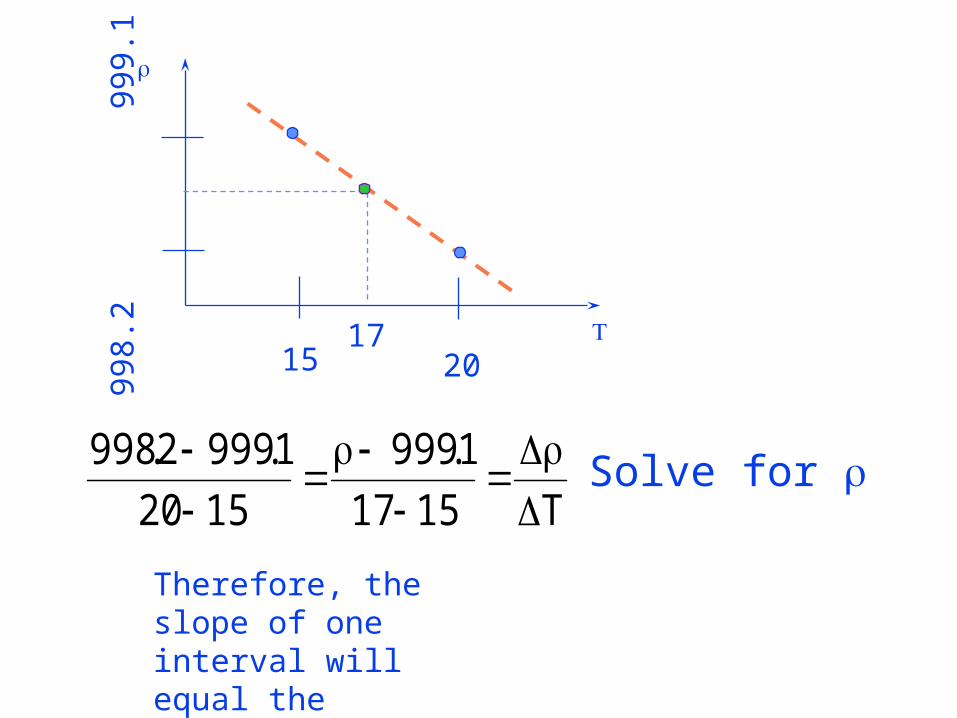
Therefore, the slope of one interval will equal theslope of the other interval.

T1517

1.999

1520

1.9992.998

Solve for

15 20

998.

2

999.

1

17

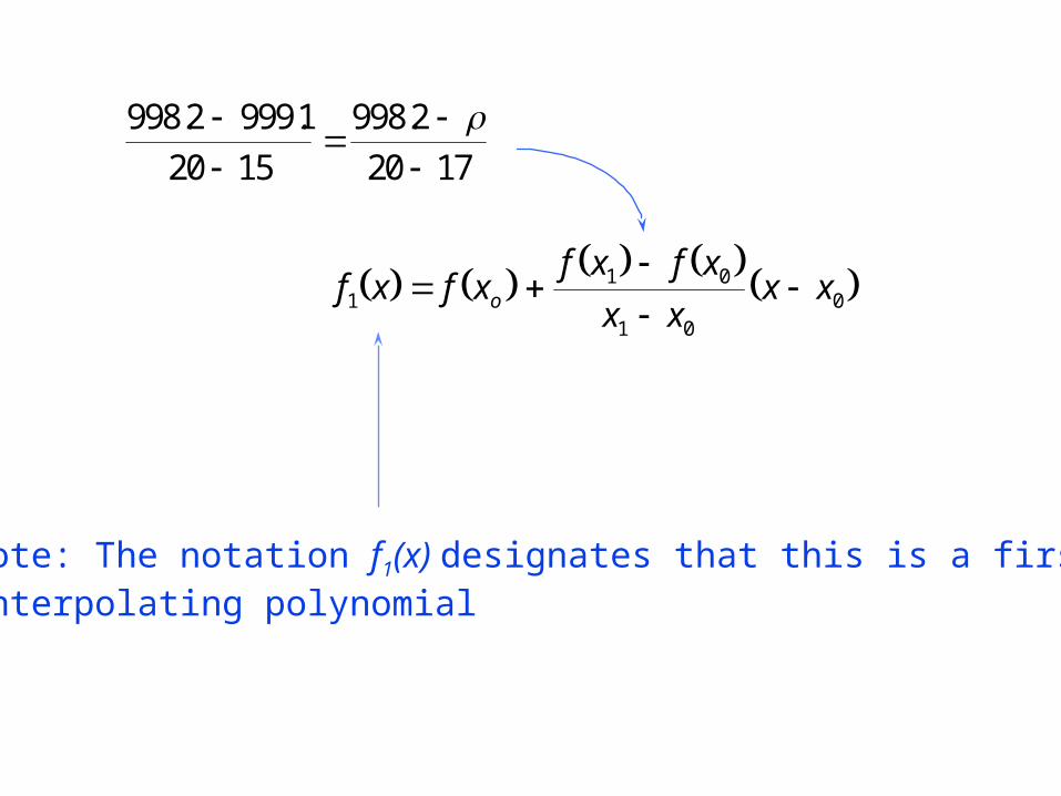
f x f xf x f x

x xx xo1

1 0

1 00

998 2 999 1

20 15

998 2

20 17

. . .

Note: The notation f1(x) designates that this is a first orderinterpolating polynomial

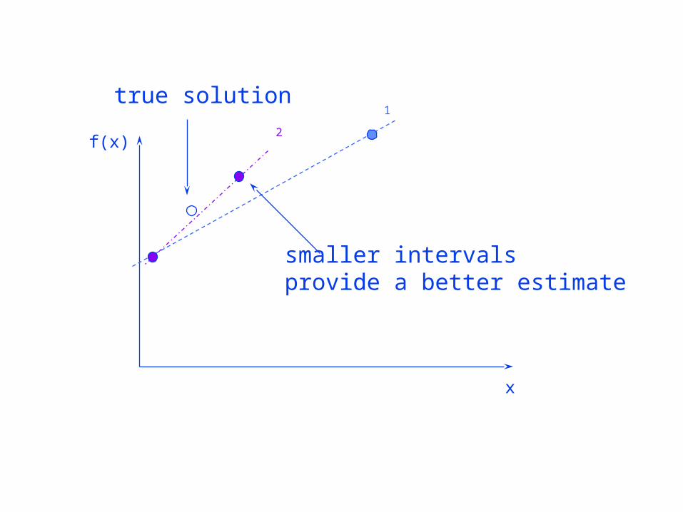
f(x)

x

true solution

smaller intervalsprovide a better estimate

1

2

f(x)

x

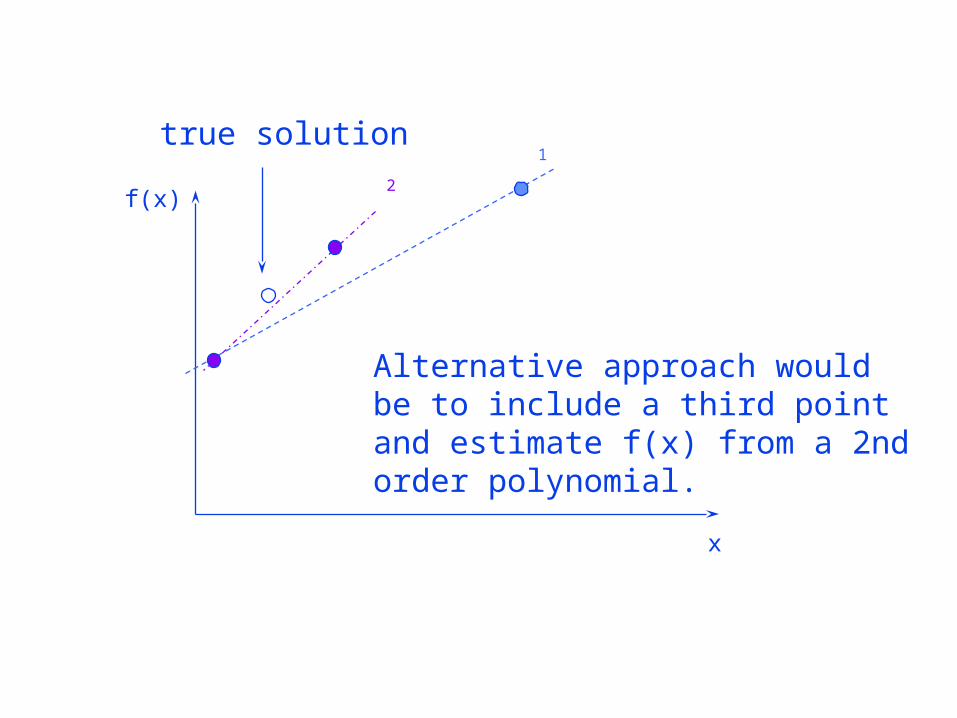
true solution1

2

Alternative approach would be to include a third point and estimate f(x) from a 2nd order polynomial.

f(x)

x

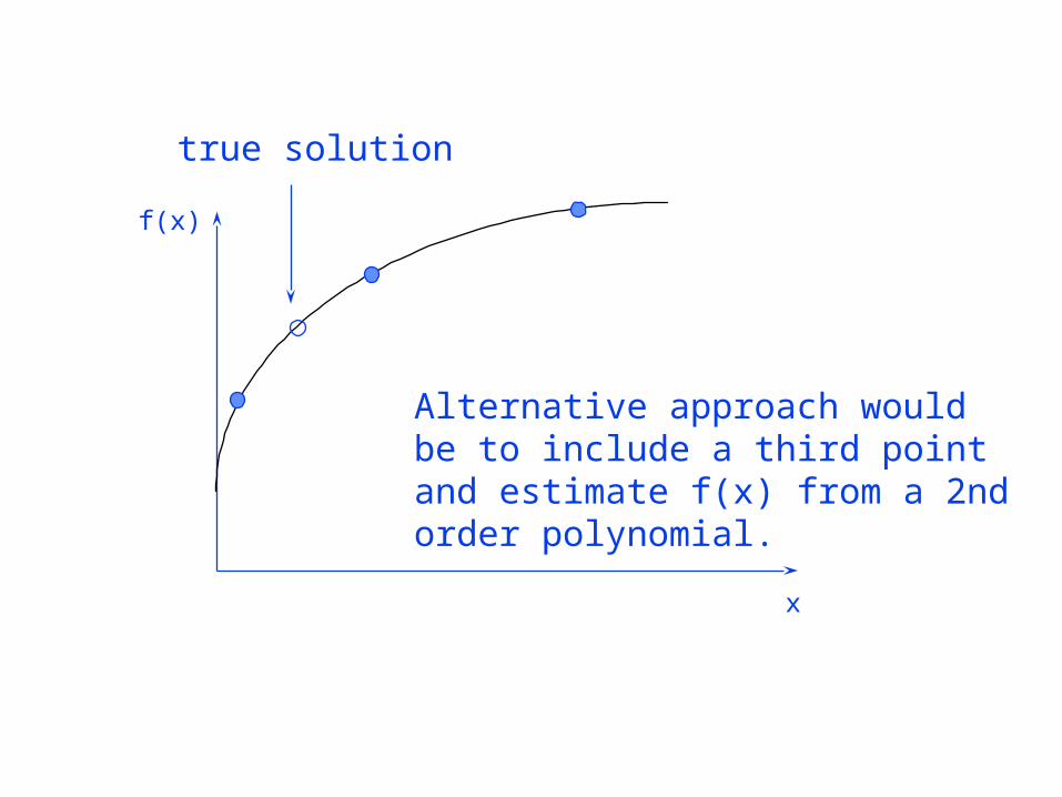
true solution

Alternative approach would be to include a third point and estimate f(x) from a 2nd order polynomial.

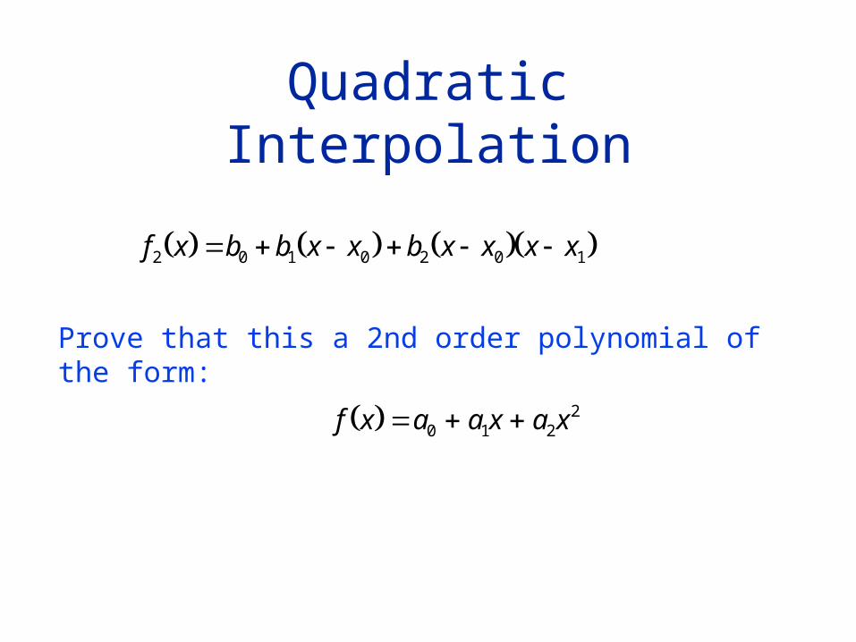
Quadratic Interpolation

f x b b x x b x x x x2 0 1 0 2 0 1

Prove that this a 2nd order polynomial ofthe form:

f x a a x a x 0 1 22

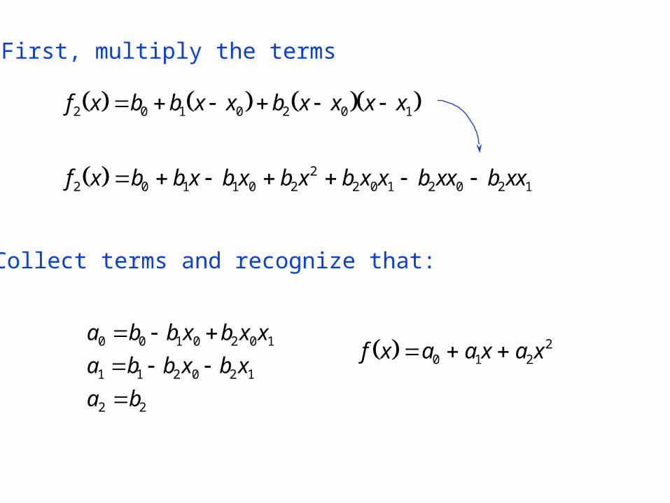
f x b b x b x b x b x x b xx b xx2 0 1 1 0 22

2 0 1 2 0 2 1

First, multiply the terms

f x a a x a x 0 1 22

f x b b x x b x x x x2 0 1 0 2 0 1

Collect terms and recognize that:

a b b x b x x

a b b x b x

a b

0 0 1 0 2 0 1

1 1 2 0 2 1

2 2

f(x)

x

x2, f(x2)

x1, f(x1)

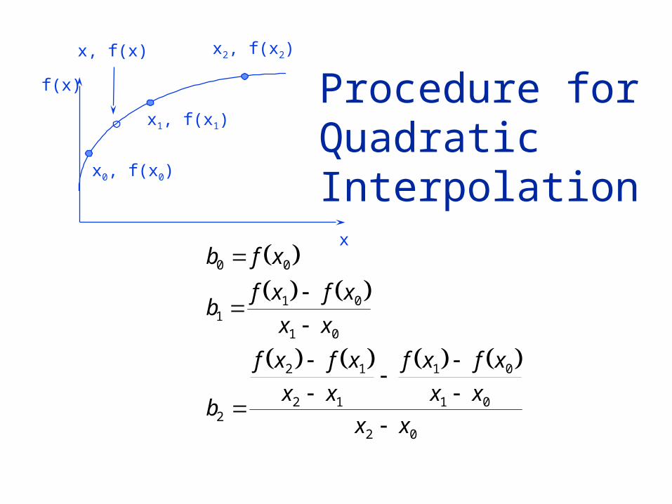
x0, f(x0)

x, f(x)

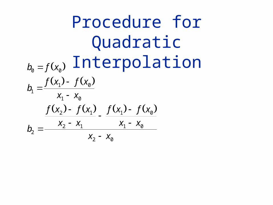
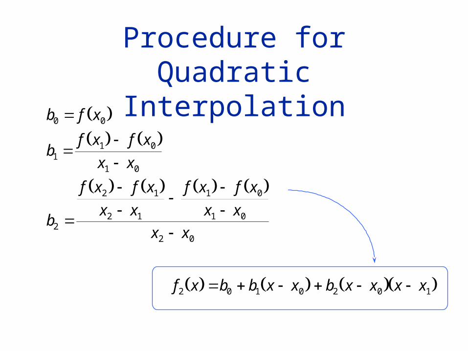
b f x

bf x f x

x x

b

f x f x

x x

f x f x

x x

x x

0 0

11 0

1 0

2

2 1

2 1

1 0

1 0

2 0

Procedure for Quadratic Interpolation

Procedure for Quadratic Interpolation

b f x

bf x f x

x x

b

f x f x

x x

f x f x

x x

x x

0 0

11 0

1 0

2

2 1

2 1

1 0

1 0

2 0

Procedure for Quadratic Interpolation

b f x

bf x f x

x x

b

f x f x

x x

f x f x

x x

x x

0 0

11 0

1 0

2

2 1

2 1

1 0

1 0

2 0

f x b b x x b x x x x2 0 1 0 2 0 1

Example

998

998.5

999

999.5

1000

0 5 10 15 20

Temp

Den

sity

Temperature, C Density, kg/m3

0 999.9

5 1000.0

10 999.7

15 999.1

20 998.2

Include 10 degrees inyour calculation of thedensity at 17 degrees.

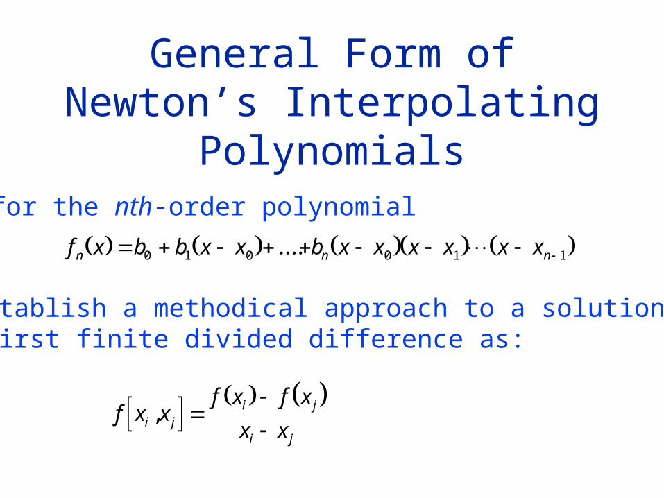
General Form of Newton’s Interpolating Polynomials

for the nth-order polynomial

f x b b x x b x x x x x xn n n 0 1 0 0 1 1....

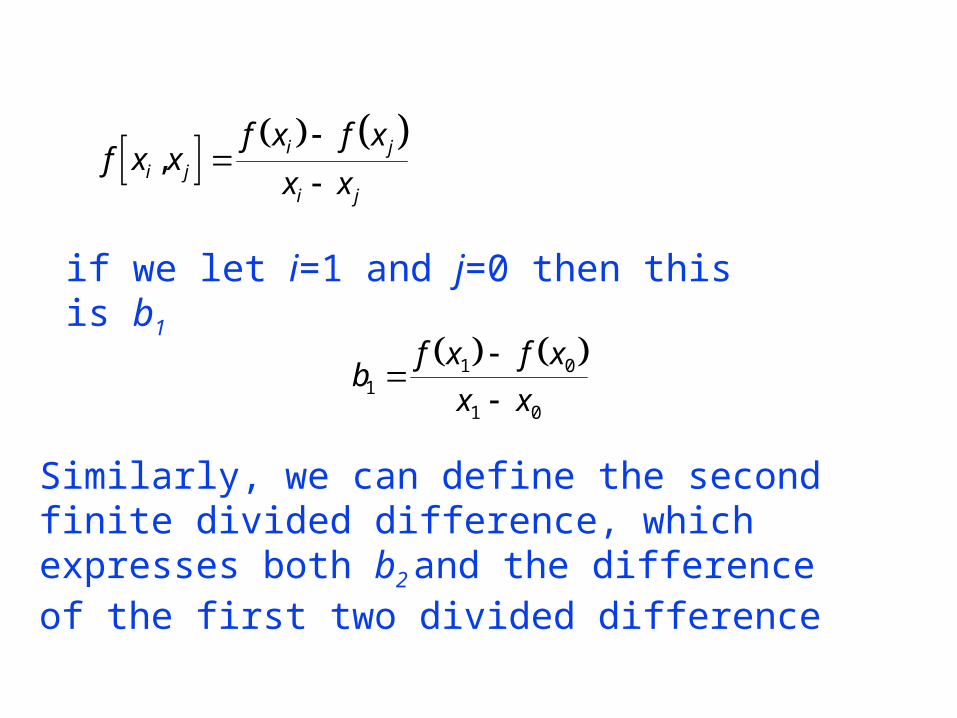
To establish a methodical approach to a solution definethe first finite divided difference as:

f x x

f x f x

x xi ji j

i j

,

f x x

f x f x

x xi ji j

i j

,

if we let i=1 and j=0 then this is b1

b

f x f x

x x11 0

1 0

Similarly, we can define the second finite divided difference, which expresses both b2 and the difference of the first two divided difference

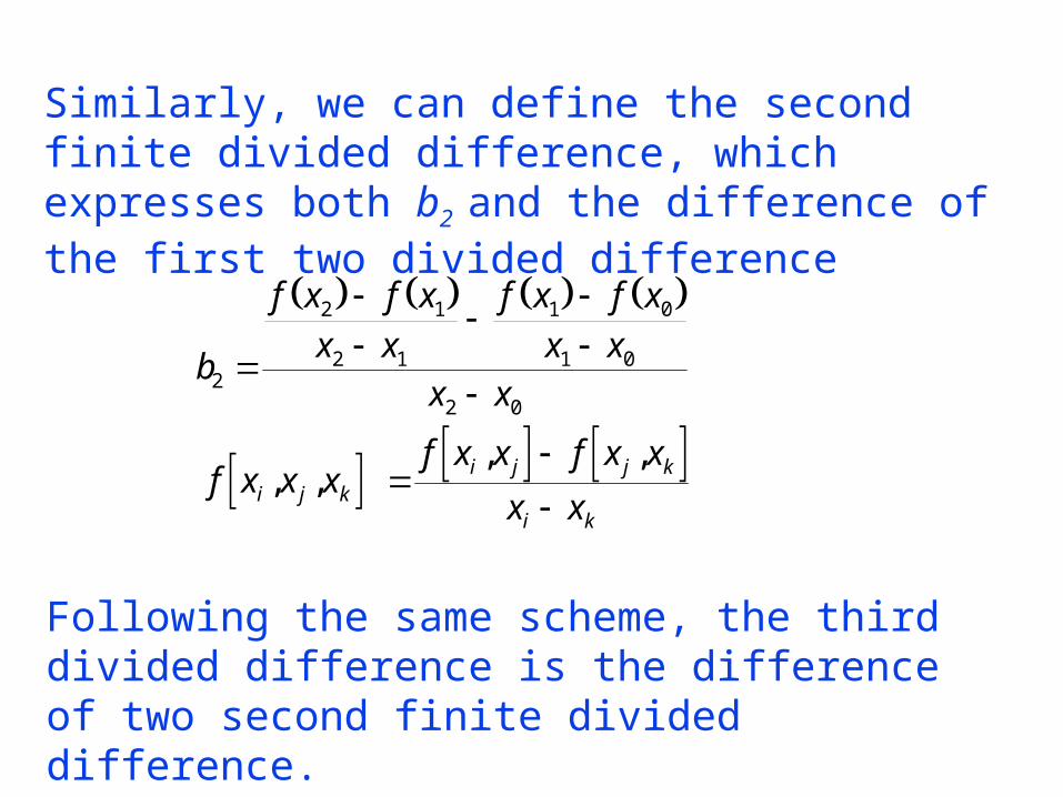
Similarly, we can define the second finite divided difference, which expresses both b2 and the difference of the first two divided difference

b

f x f x

x x

f x f x

x xx x

f x x xf x x f x x

x xi j ki j j k

i k

2

2 1

2 1

1 0

1 0

2 0

, ,, ,

Following the same scheme, the third divided difference is the difference of two second finite divided difference.

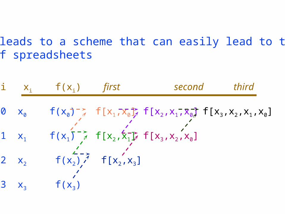
This leads to a scheme that can easily lead to theuse of spreadsheets

i xi f(xi) first second third

0 x0 f(x0) f[x1,x0] f[x2,x1,x0] f[x3,x2,x1,x0]

1 x1 f(x1) f[x2,x1] f[x3,x2,x0]

2 x2 f(x2) f[x2,x3] 3 x3 f(x3)

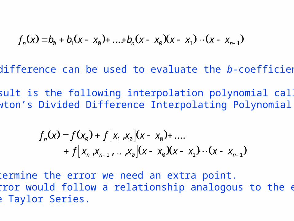
f x b b x x b x x x x x xn n n 0 1 0 0 1 1....

These difference can be used to evaluate the b-coefficients.

The result is the following interpolation polynomial calledthe Newton’s Divided Difference Interpolating Polynomial

f x f x f x x x x

f x x x x x x x x xn

n n n

0 1 0 0

1 0 0 1 1

, ....

, , ,

To determine the error we need an extra point.The error would follow a relationship analogous to the errorin the Taylor Series.

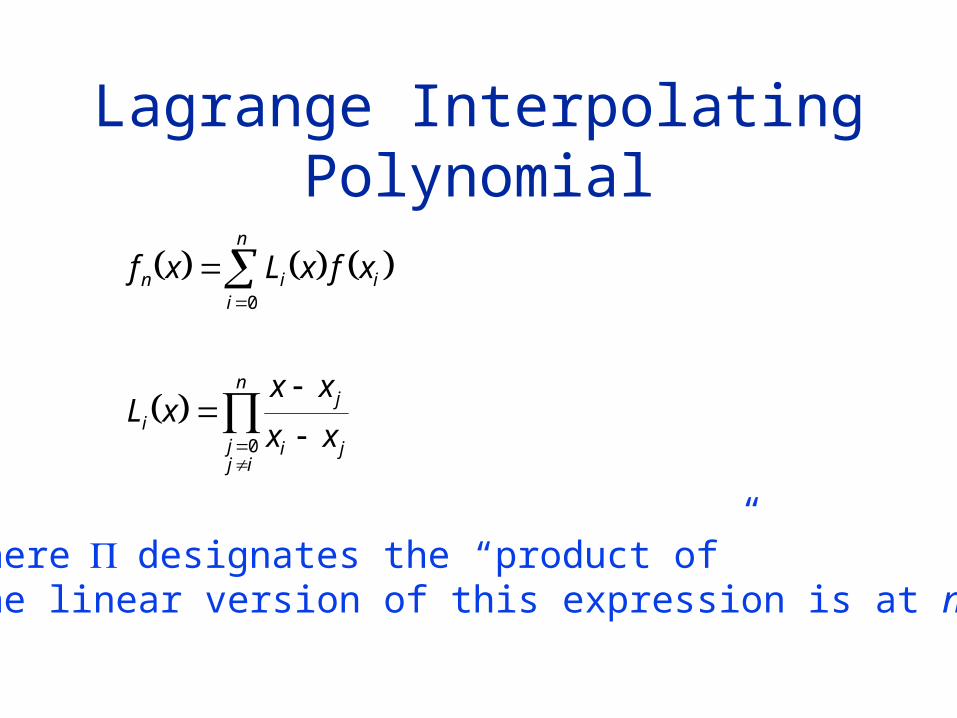
Lagrange Interpolating Polynomial

f x L x f x

L xx x

x x

n i ii

n

ij

i jjj i

n

0

0

wheredesignates the “product of”The linear version of this expression is at n=1

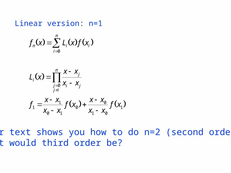
f x L x f x

L xx x

x x

fx x

x xf x

x x

x xf x

n i ii

n

ij

i jjj i

n

0

0

11

0 10

0

1 01

Linear version: n=1

Your text shows you how to do n=2 (second order).What would third order be?

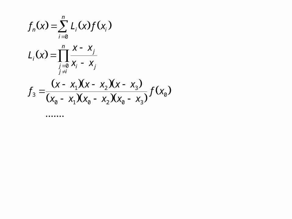
f x L x f x

L xx x

x x

fx x x x x x

x x x x x xf x

n i ii

n

ij

i jjj i

n

0

0

31 2 3

0 1 0 2 0 30

.......

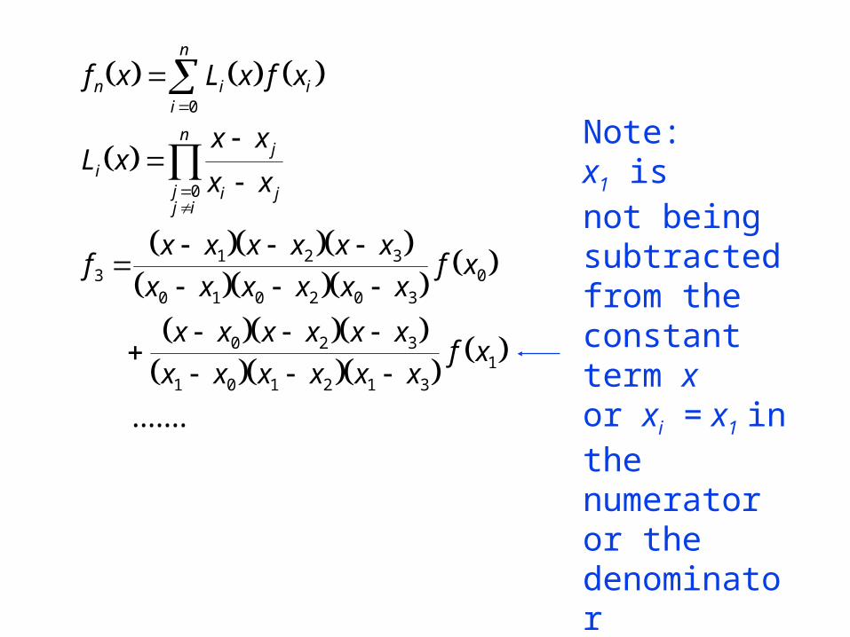
f x L x f x

L xx x

x x

fx x x x x x

x x x x x xf x

x x x x x x

x x x x x xf x

n i ii

n

ij

i jjj i

n

0

0

31 2 3

0 1 0 2 0 30

0 2 3

1 0 1 2 1 31

.......

Note:x1 isnot being subtractedfrom the constantterm x or xi = x1 inthe numeratoror the denominatorj= 1

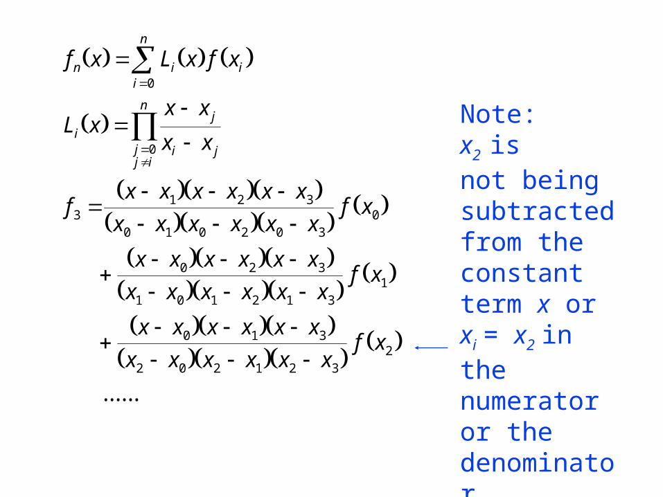
f x L x f x

L xx x

x x

fx x x x x x

x x x x x xf x

x x x x x x

x x x x x xf x

x x x x x x

x x x x x xf x

n i ii

n

ij

i jjj i

n

0

0

31 2 3

0 1 0 2 0 30

0 2 3

1 0 1 2 1 31

0 1 3

2 0 2 1 2 32

......

Note:x2 isnot being subtractedfrom the constantterm x or xi = x2 inthe numeratoror the denominatorj= 2

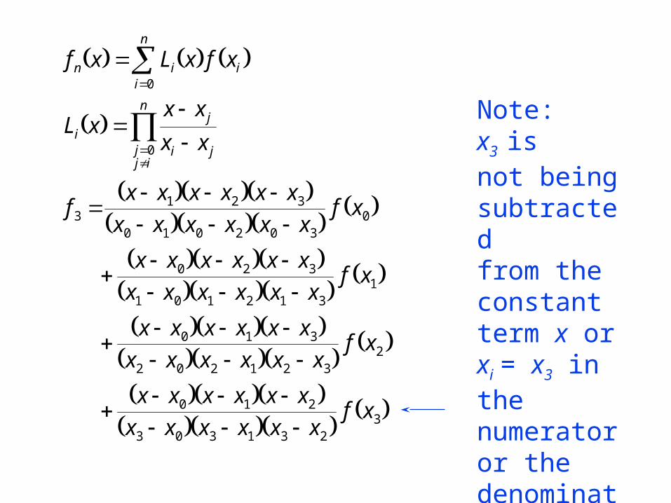
f x L x f x

L xx x

x x

fx x x x x x

x x x x x xf x

x x x x x x

x x x x x xf x

x x x x x x

x x x x x xf x

x x x x x x

x x x x x xf x

n i ii

n

ij

i jjj i

n

0

0

31 2 3

0 1 0 2 0 30

0 2 3

1 0 1 2 1 31

0 1 3

2 0 2 1 2 32

0 1 2

3 0 3 1 3 23

Note:x3 isnot being subtractedfrom the constantterm x or xi = x3 inthe numeratoror the denominatorj= 3

Example

998

998.5

999

999.5

1000

0 5 10 15 20

Temp

Den

sity

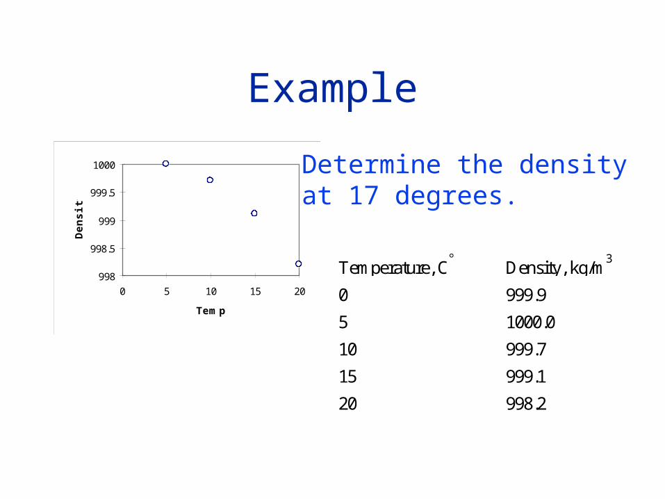
Temperature, C Density, kg/m3

0 999.9

5 1000.0

10 999.7

15 999.1

20 998.2

Determine the densityat 17 degrees.

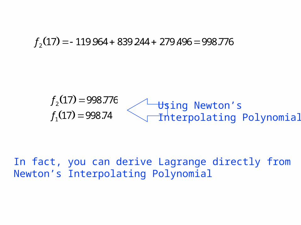
In fact, you can derive Lagrange directly fromNewton’s Interpolating Polynomial

f 2 17 119.964 839.244 279.496 998 776 .

f

f2

1

17 998 776

17 998 74

.

.Using Newton’sInterpolating Polynomial

Coefficients of an Interpolating Polynomial

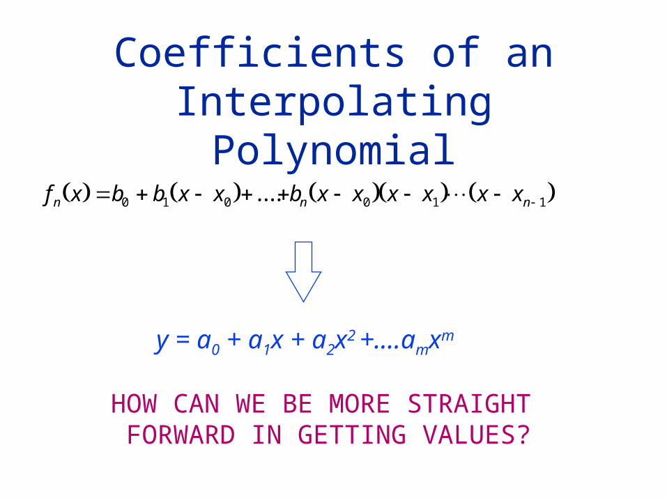
f x b b x x b x x x x x xn n n 0 1 0 0 1 1....

y = a0 + a1x + a2x2 +....amxm

HOW CAN WE BE MORE STRAIGHT FORWARD IN GETTING VALUES?

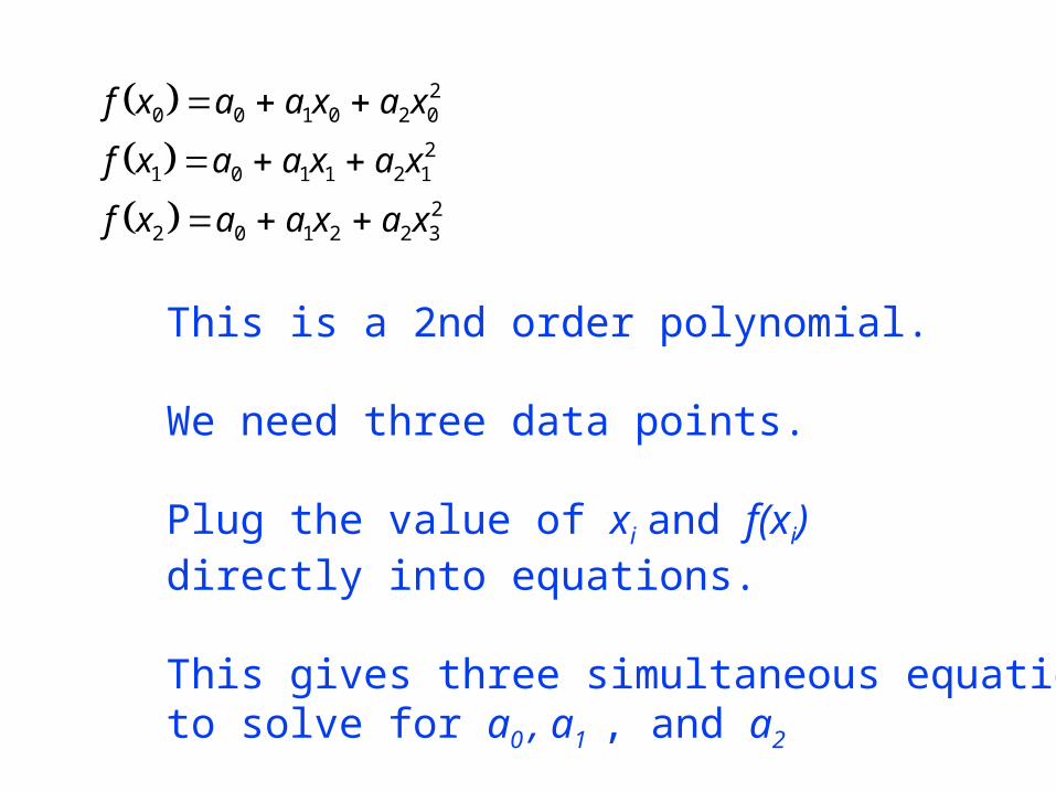
f x a a x a x

f x a a x a x

f x a a x a x

0 0 1 0 2 02

1 0 1 1 2 12

2 0 1 2 2 32

This is a 2nd order polynomial.

We need three data points.

Plug the value of xi and f(xi)directly into equations.

This gives three simultaneous equationsto solve for a0 , a1 , and a2

Example

998

998.5

999

999.5

1000

0 5 10 15 20

Temp

Den

sity

Temperature, C Density, kg/m3

0 999.9

5 1000.0

10 999.7

15 999.1

20 998.2

Determine the densityat 17 degrees.

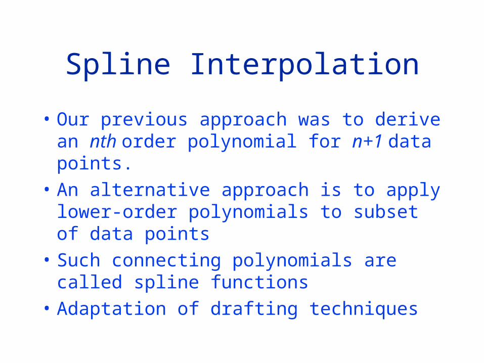
Spline Interpolation

• Our previous approach was to derive an nth order polynomial for n+1 data points.

• An alternative approach is to apply lower-order polynomials to subset of data points

• Such connecting polynomials are called spline functions

• Adaptation of drafting techniques

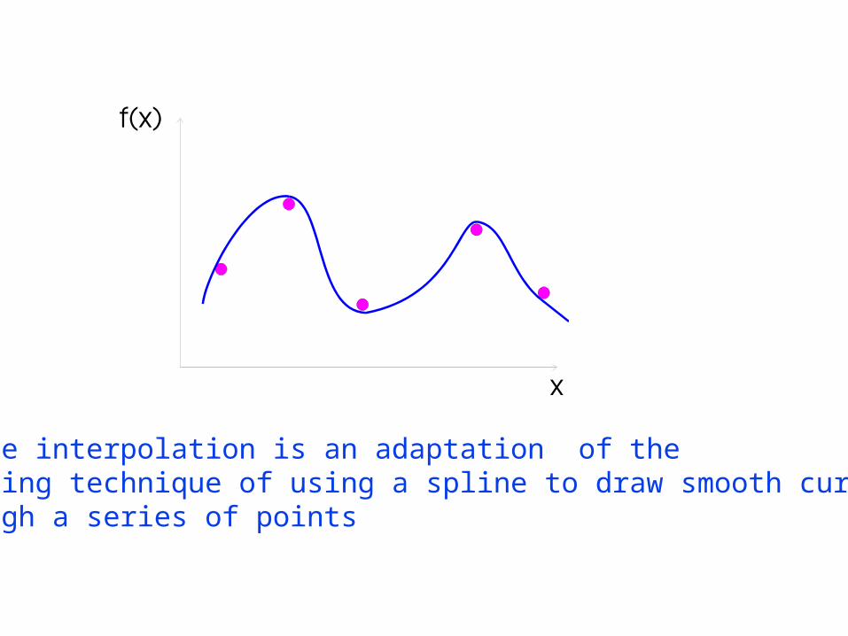
Spline interpolation is an adaptation of thedrafting technique of using a spline to draw smooth curvesthrough a series of points

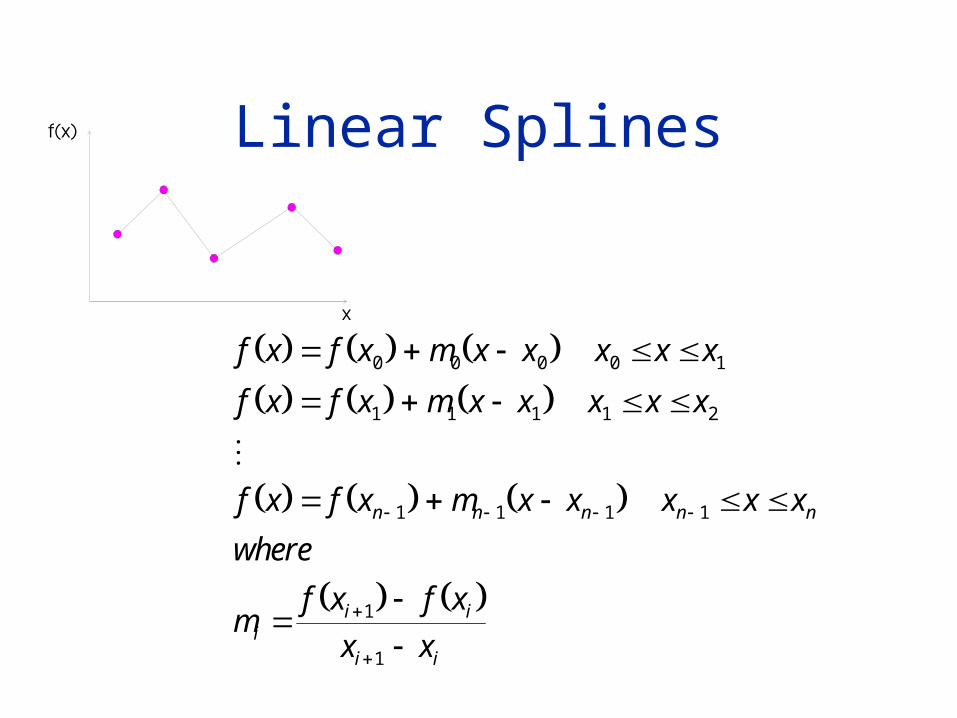
Linear Splines

f x f x m x x x x x

f x f x m x x x x x

f x f x m x x x x x

where

mf x f x

x x

n n n n n

ii i

i i

0 0 0 0 1

1 1 1 1 2

1 1 1 1

1

1

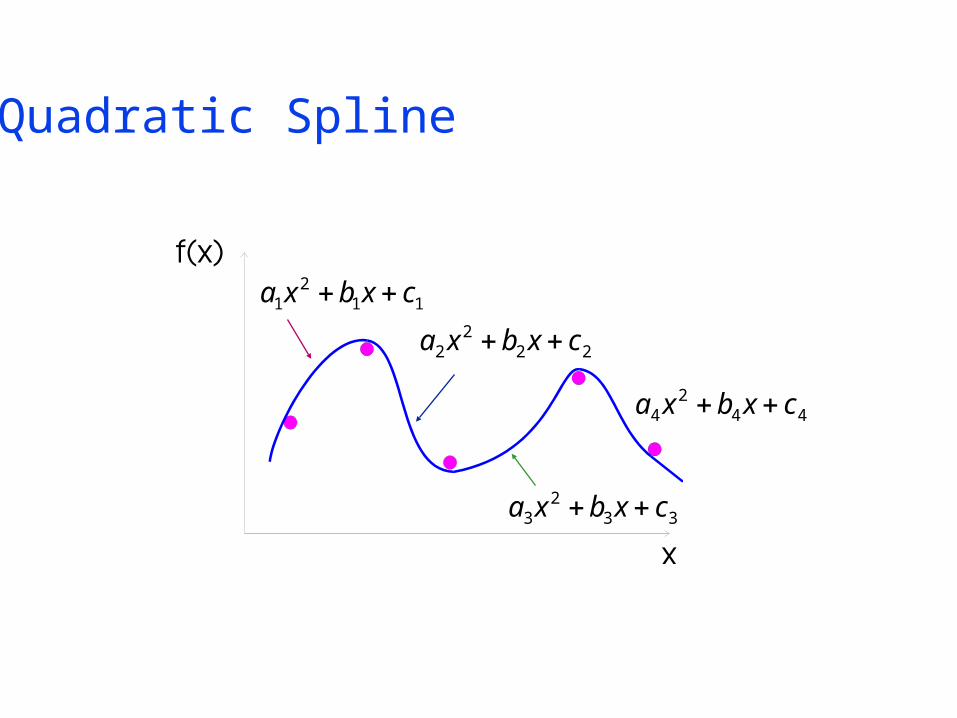
Quadratic Spline

112

1 cxbxa

222

2 cxbxa

332

3 cxbxa

442

4 cxbxa

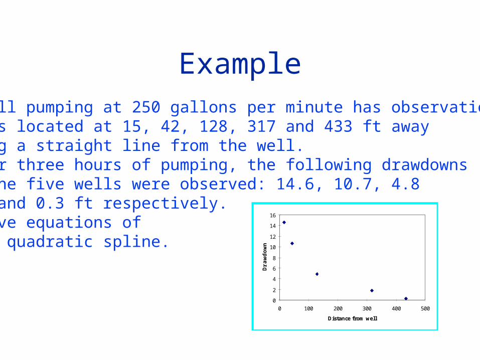
ExampleA well pumping at 250 gallons per minute has observationwells located at 15, 42, 128, 317 and 433 ft awayalong a straight line from the well.After three hours of pumping, the following drawdownsin the five wells were observed: 14.6, 10.7, 4.81.7 and 0.3 ft respectively.Derive equations of each quadratic spline.

0

2

4

6

8

10

12

14

16

0 100 200 300 400 500

Distance from well

Dra

wdo

wn

Splines• To ensure that the mth derivatives are continuous

at the “knots”, a spline of at least m+1 order must be used

• 3rd order polynomials or cubic splines that ensure continuous first and second derivatives are most frequently used in practice

• Although third and higher derivatives may be discontinuous when using cubic splines, they usually cannot be detected visually and consequently are ignored.

Splines

• The derivation of cubic splines is somewhat involved

• First illustrate the concepts of spline interpolation using second order polynomials.

• These “quadratic splines” have continuous first derivatives at the “knots”

• Note: This does not ensure equal second derivatives at the “knots”

Quadratic Spline

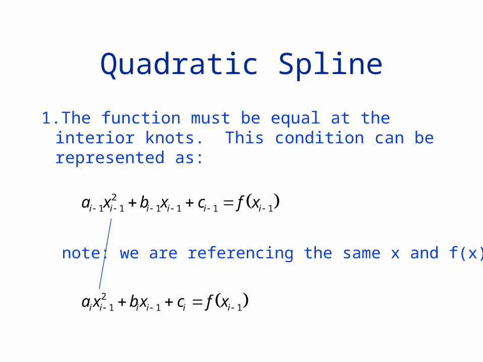
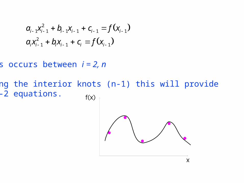
1.The function must be equal at the interior knots. This condition can be represented as:

a x b x c f x

a x b x c f x

i i i i i i

i i i i i i

1 12

1 1 1 1

12

1 1

note: we are referencing the same x and f(x)

a x b x c f x

a x b x c f x

i i i i i i

i i i i i i

1 1

21 1 1 1

12

1 1

This occurs between i = 2, n

Using the interior knots (n-1) this will provide2n -2 equations.

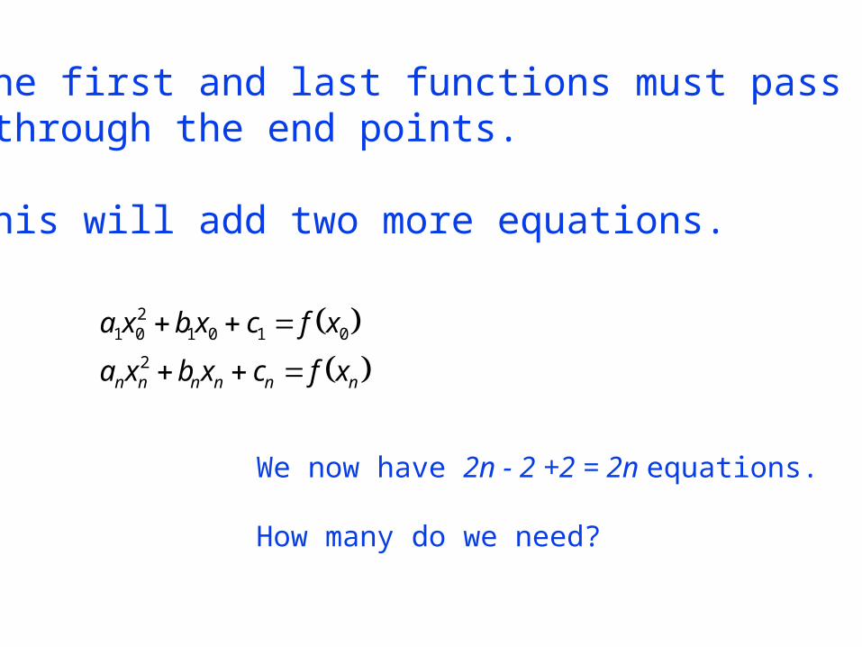
2. The first and last functions must pass through the end points.

This will add two more equations.

a x b x c f x

a x b x c f xn n n n n n

1 02

1 0 1 0

2

We now have 2n - 2 +2 = 2n equations.

How many do we need?

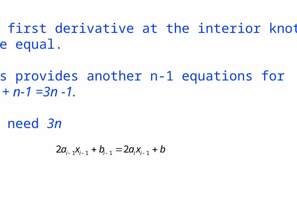
3. The first derivative at the interior knots must be equal.

This provides another n-1 equations for 2n + n-1 =3n -1.

We need 3n

2 21 1 1 1a x b a x bi i i i i

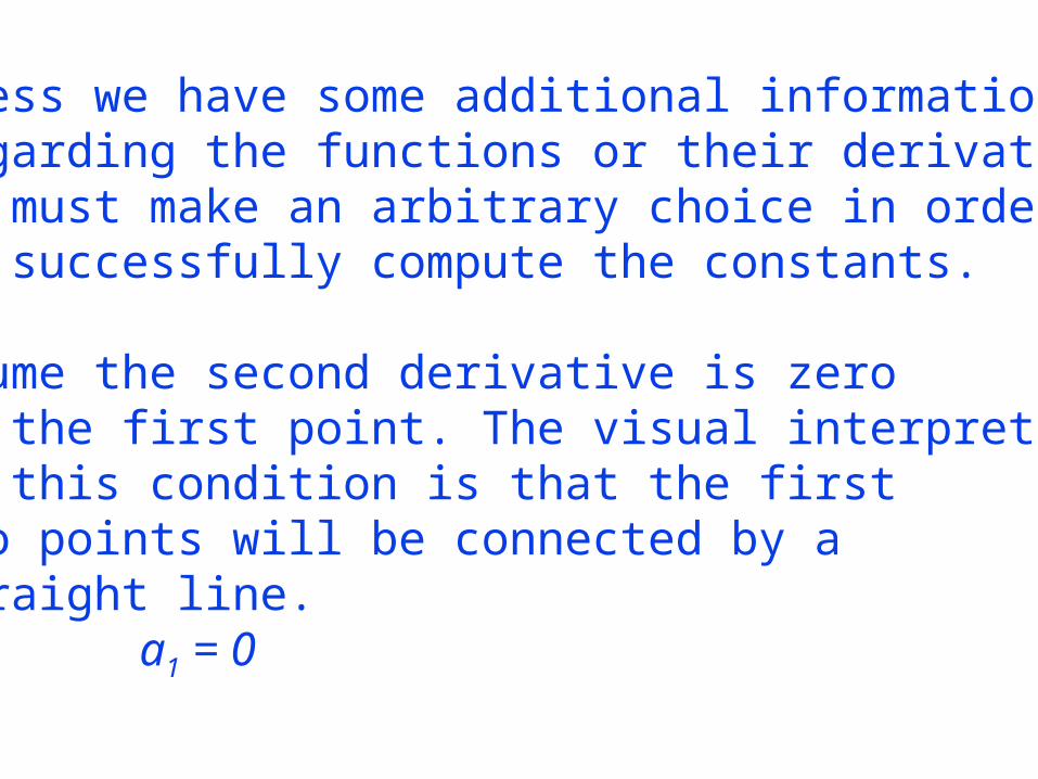
4. Unless we have some additional information regarding the functions or their derivatives, we must make an arbitrary choice in order to successfully compute the constants.

5. Assume the second derivative is zero at the first point. The visual interpretation of this condition is that the first two points will be connected by a straight line. a1 = 0

Cubic Splines

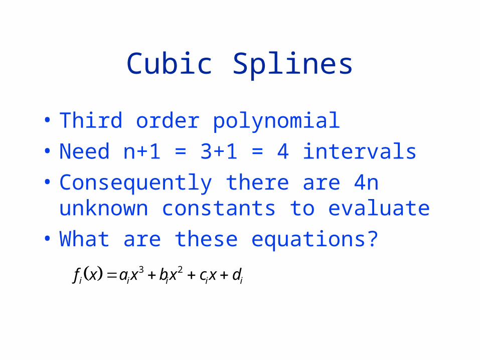
• Third order polynomial

• Need n+1 = 3+1 = 4 intervals

• Consequently there are 4n unknown constants to evaluate

• What are these equations?

f x a x b x c x di i i i i 3 2

Cubic Splines

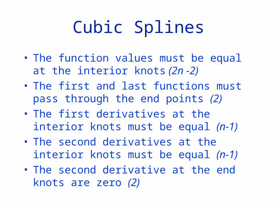
• The function values must be equal at the interior knots (2n -2)

• The first and last functions must pass through the end points (2)

• The first derivatives at the interior knots must be equal (n-1)

• The second derivatives at the interior knots must be equal (n-1)

• The second derivative at the end knots are zero (2)

Cubic Splines

• The function values must be equal at the interior knots (2n -2)

• The first and last functions must pass through the end points (2)

• The first derivatives at the interior knots must be equal (n-1)

• The second derivatives at the interior knots must be equal (n-1)

• The second derivative at the end knots are zero (2)

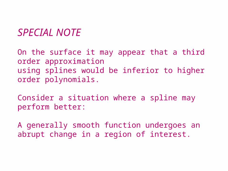
SPECIAL NOTE

On the surface it may appear that a third order approximationusing splines would be inferior to higher order polynomials.

Consider a situation where a spline may perform better:

A generally smooth function undergoes an abrupt change in a region of interest.

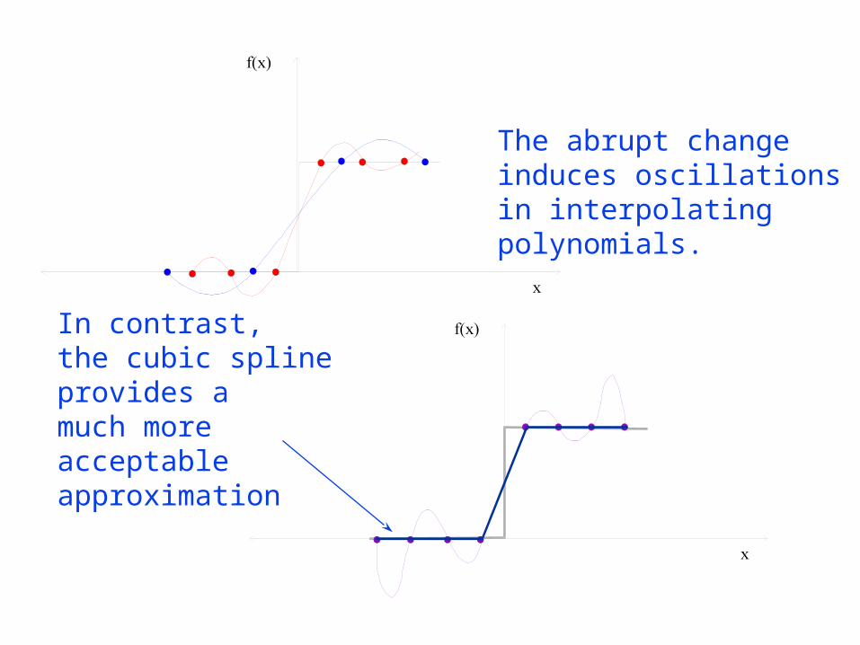
The abrupt changeinduces oscillationsin interpolating polynomials.

In contrast,the cubic splineprovides amuch moreacceptableapproximation

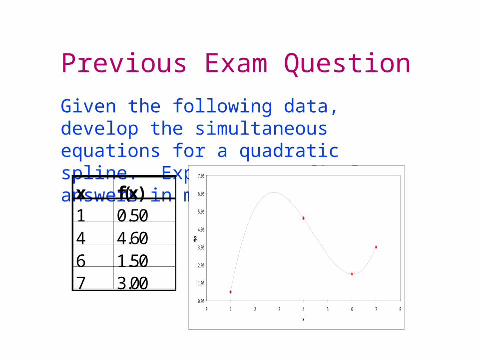
Previous Exam Question

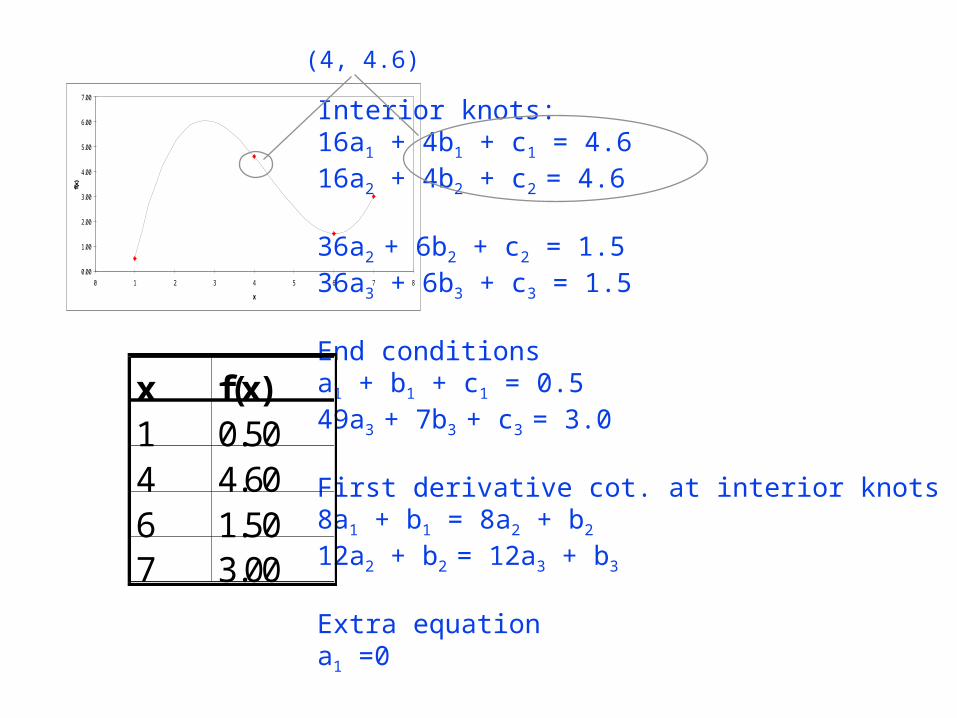
Given the following data, develop the simultaneous equations for a quadratic spline. Express your final answers in matrix form.

x f(x)1 0.504 4.606 1.507 3.00

0.00

1.00

2.00

3.00

4.00

5.00

6.00

7.00

0 1 2 3 4 5 6 7 8

x

f(x)

0.00

1.00

2.00

3.00

4.00

5.00

6.00

7.00

0 1 2 3 4 5 6 7 8

x

f(x)

Interior knots:16a1 + 4b1 + c1 = 4.616a2 + 4b2 + c2 = 4.6

36a2 + 6b2 + c2 = 1.536a3 + 6b3 + c3 = 1.5

End conditionsa1 + b1 + c1 = 0.549a3 + 7b3 + c3 = 3.0

First derivative cot. at interior knots8a1 + b1 = 8a2 + b2

12a2 + b2 = 12a3 + b3

Extra equationa1 =0

x f(x)1 0.504 4.606 1.507 3.00

(4, 4.6)

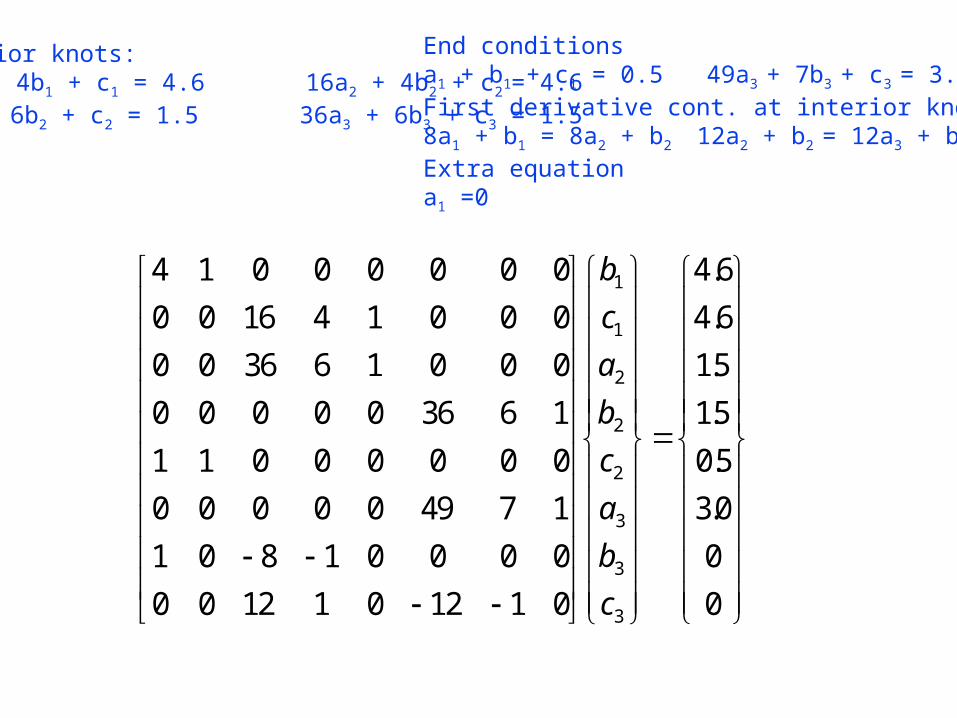
Interior knots:16a1 + 4b1 + c1 = 4.6 16a2 + 4b2 + c2 = 4.636a2 + 6b2 + c2 = 1.5 36a3 + 6b3 + c3 = 1.5

4 1 0 0 0 0 0 0

0 0 16 4 1 0 0 0

0 0 36 6 1 0 0 0

0 0 0 0 0 36 6 1

1 1 0 0 0 0 0 0

0 0 0 0 0 49 7 1

1 0 8 1 0 0 0 0

0 0 12 1 0 12 1 0

4.6

4.6

15

15

0 5

3 0

0

0

1

1

2

2

2

3

3

3

b

c

a

b

c

a

b

c

.

.

.

.

End conditionsa1 + b1 + c1 = 0.5 49a3 + 7b3 + c3 = 3.0First derivative cont. at interior knots8a1 + b1 = 8a2 + b2 12a2 + b2 = 12a3 + b3

Extra equationa1 =0