Embed Size (px)
Citation preview
Prepared for submission to JCAP
Curvature radius and Kerr black holeshadow
Shao-Wen Wei1,2, Yuan-Chuan Zou3,4, Yu-Xiao Liu1, Robert B.Mann2
1Institute of Theoretical Physics & Research Center of Gravitation, Lanzhou University,Lanzhou 730000, People’s Republic of China2Department of Physics and Astronomy, University of Waterloo, Waterloo, Ontario, Canada,N2L 3G13School of Physics, Huazhong University of Science and Technology, Wuhan 430074, Peo-ple’s Republic of China4Perimeter Institute, 31 Caroline St., Waterloo, Ontario, N2L 2Y5, Canada
E-mail: [email protected], [email protected], [email protected],[email protected]
Abstract. We consider applications of the curvature radius of a Kerr black hole shadow andpropose three new approaches to simultaneously determine the black hole spin and inclinationangle of the observer. The first one uses only two symmetric characteristic points, i.e., thetop and the bottom points of the shadow, and is the smallest amount of data employed toextract information about spin and inclination angle amongst all current treatments. Thesecond approach shows that only measuring the curvature radius at the characteristic pointscan also yield the black hole spin and the inclination angle. The observables used in thethird approach have large changes to the spin and the inclination angle, which may give us amore accurate way to determine these parameters. Moreover, by modeling the supermassiveblack hole M87* with a Kerr black hole, we calculate the angular size for these curvatureradii of the shadow. Some novel properties are found and analyzed. The results may shinenew light on the relationship between the curvature radius and the black hole shadow, andprovide several different approaches to test the nature of the black hole through the shadow.
Keywords: Black holes, shadow, null geodesics
arX
iv:1
904.
0771
0v2
[gr
-qc]
26
Sep
2019
Contents
1 Introduction 1
2 Null geodesics and shadow 2
3 Determining spin and inclination angle 43.1 Approach I 43.2 Approach II 83.3 Approach III 9
4 Application to M87* 10
5 Conclusions and discussions 11
1 Introduction
Very recently, the Event Horizon Telescope (EHT) has showcased the first image of thesupermassive black hole M87* [1–3]. This fruitful outcome reveals a fine structure nearthe black hole horizon. The photon ring and shadow have been clearly observed, whichprovides us with a good opportunity to test general relativity in the regime of strong gravity.Combined with upcoming telescope surveys, such as the Next Generation Very Large Array[4] and the Thirty Meter Telescope [5], more high-resolution observations will yield importantnew information about strong gravity.
A black hole shadow is a two dimensional dark zone in the celestial sphere caused bythe strong gravity of the black hole. It was first studied by Synge in 1966 for a Schwarzschildblack hole [6]. Later, a formula for the angular radius for the shadow was given by Luminet[7]. In general, the shadow cast by a non-rotating black hole is a standard circle, whereas fora rotating black hole the shadow will be elongated in the direction of the rotating axis dueto spacetime dragging effects [8, 9]. In order to match astronomical observations, Hioki andMaeda [10] proposed two observables based on the characteristic points on the boundary ofthe Kerr shadow. One approximately describes the size of the shadow, and another describesthe deformation of its shape from a reference circle. This approach has been extended toother black holes [11–42], and a coordinate-independent study of the shadow by making useof Legendre polynomials has been carried out [43].
Information about the properties of a black hole is contained on the boundary of itsshadow. So if the boundary curve is uniquely determined, we can extract this informationfrom it. Motivated by this idea we recently introduced a new concept, the local curvatureradius [39], from the viewpoint of differential geometry. For each fixed black hole spin andinclination angle of the observer, we found there exists one minimum and one maximumof the curvature radius upon taking the symmetry of the black hole shadow into account.Employing this property we showed that both the spin and the inclination angle can beuniquely determined.
We further extended our application of the local curvature radius to construct a topo-logical quantity [39] associated with the shadow. The value of this quantity is unity for anarbitrary Kerr black hole, but smaller than one for a naked singularity. Using this quantity,
– 1 –
we can therefore distinguish a black hole from a naked singularity. It can be used to measurethe topological structure for the multi-shadows in some special spacetimes.
The aim of this paper is to further explore applications of the local curvature radius.Noting that the maximum curvature always occurs at the left point of the shadow whereasthe corresponding point of the minimum curvature varies with the black hole parameters[39], we focus on how to extract black hole parameters from this information. Rather thanmeasuring the curvature radius at every point on the shadow boundary, we can exploit thesymmetry of the shadow to obtain its characteristic points, making use of a detailed studywe have previously carried out [44]. In the Kerr spacetime, these points have analyticalcoordinates for the equatorial observer, and away from the equatorial plane these points arealso very easy to work out.
It is therefore natural to combine the curvature radius and characteristic points todetermine the black hole parameters. Three novel approaches are presented in this paper.These results demonstrate that the local curvature radius is a very useful tool in the study ofblack hole shadows. We apply our results on the curvature radius to the supermassive blackhole M87*.
Our paper is organized as follows. In Sec. 2, we briefly review the null geodesics andshadow for the Kerr black hole. Then the curvature radius is introduced. In Sec. 3, we showhow to determine the black hole spin and the inclination angle of the observer by makinguse the curvature radius. Three approaches are proposed for different purposes. We thenconsider the supermassive M87* black hole in Sec. 4. Finally, the conclusions and discussionsare presented in Sec. 5.
2 Null geodesics and shadow
Here we provide a brief review of the null geodesics and shapes of the shadow in a Kerrspacetime.
In Boyer-Lindquist coordinates, the line element in a Kerr spacetime is
ds2 = −(
1− 2Mr
ρ2
)dt2 +
ρ2
∆dr2 + ρ2dθ2 − 4Mra sin2 θ
ρ2dtdφ+
((r2 + a2)2 −∆a2 sin2 θ) sin2 θ
ρ2dφ2,(2.1)
where the metric functions are
∆ = r2 − 2Mr + a2, ρ2 = r2 + a2 cos2 θ. (2.2)
The parameters M and a are, respectively, the black hole mass and spin. The horizons in aKerr spacetime can be obtained by solving ∆(r) = 0, which are located at
r± = M ±√M2 − a2. (2.3)
There are two horizons for |a| < M and one horizon for |a| = M ; no horizon exists for|a| > M , which corresponds to a naked singularity.
– 2 –
The null geodesics in the Kerr spacetime are given by the solutions to the equations
ρ2dt
dλ= a(l − aE sin2 θ) +
r2 + a2
∆
(E(r2 + a2)− al
), (2.4)
ρ2dr
dλ=√<, (2.5)
ρ2dθ
dλ=√
Θ, (2.6)
ρ2dφ
dλ= (l csc2 θ − aE) +
a
∆
(E(r2 + a2)− al
), (2.7)
where λ is the affine parameter. The functions < and Θ are given by
< =(a2E − al + Er2
)2 −∆(Q+ (l − aE)2
), (2.8)
Θ = Q− (l csc θ − aE sin θ)2 + (l − aE)2. (2.9)
Here the conserved quantities l and E are the angular momentum and energy of the testparticle, which are related with the Killing vector fields ∂φ and ∂t, respectively. The conservedCarter constant Q is related to the Killing-Yano tensor field in the Kerr spacetime [45, 46].Moreover, one can introduce two new parameters ξ and η
ξ =l
E, η =
QE2
. (2.10)
By making use of the null geodesics, we can obtain the two celestial coordinates α and β,which are used to describe the shape of the shadow that an observer seen in the sky. For anobserver of the inclination angle θ0, the celestial coordinates are given by
α = −ξ csc θ0, (2.11)
β = ±√η + a2 cos2 θ0 − ξ2 cot2 θ0. (2.12)
On the boundary, the parameters ξ and η are given by [47]
ξ =(3M − r0)r20 − a2(M + r0)
a(r0 −M), (2.13)
η =r30(4a2M − r0(3M − r0)2)
a2(r0 −M)2. (2.14)
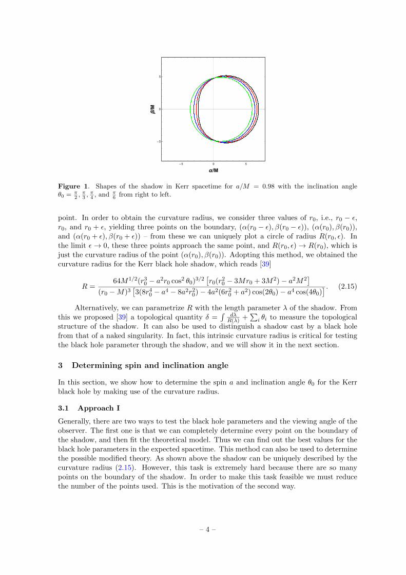
where r0 varies between the light ring radii of direct and retrograde photons along the bound-ary of the shadow. This also provides us with a parametrization of the form of the shadow,and based on it, some analytic results can be obtained Ref. [44]. For convenience, we showthe shapes of the shadow for the black hole in Fig. 1 with spin a/M = 0.98, and inclinationangle θ0 = π
2 ,π3 ,
π4 , and π
6 from right to left. In order to study them, we introduced a newquantity, the curvature radius R [39]. From the viewpoint of differential geometry, if wemeasure the curvature radius at each point of the boundary, the shadow will be uniquely de-termined, and then we can exactly read out the black hole parameters in a given spacetime,or to distinguish different gravity theories via the structure of the shadow.
We now briefly review how to calculate the local curvature radius [39]. From Eqs.(2.11) and (2.12), one can find that the celestial coordinates (α, β) for each point on theboundary of the shadow are parametrized by r0. Thus each value of r0 corresponds to one
– 3 –
-5 0 5
-5
0
5
α/M
β/M
Figure 1. Shapes of the shadow in Kerr spacetime for a/M = 0.98 with the inclination angleθ0 = π
2 ,π3 ,
π4 , and π
6 from right to left.
point. In order to obtain the curvature radius, we consider three values of r0, i.e., r0 − ε,r0, and r0 + ε, yielding three points on the boundary, (α(r0 − ε), β(r0 − ε)), (α(r0), β(r0)),and (α(r0 + ε), β(r0 + ε)) – from these we can uniquely plot a circle of radius R(r0, ε). Inthe limit ε→ 0, these three points approach the same point, and R(r0, ε)→ R(r0), which isjust the curvature radius of the point (α(r0), β(r0)). Adopting this method, we obtained thecurvature radius for the Kerr black hole shadow, which reads [39]
R =64M1/2(r30 − a2r0 cos2 θ0)
3/2[r0(r
20 − 3Mr0 + 3M2)− a2M2
](r0 −M)3
[3(8r40 − a4 − 8a2r20)− 4a2(6r20 + a2) cos(2θ0)− a4 cos(4θ0)
] . (2.15)
Alternatively, we can parametrize R with the length parameter λ of the shadow. Fromthis we proposed [39] a topological quantity δ =
∫dλR(λ) +
∑i θi to measure the topological
structure of the shadow. It can also be used to distinguish a shadow cast by a black holefrom that of a naked singularity. In fact, this intrinsic curvature radius is critical for testingthe black hole parameter through the shadow, and we will show it in the next section.
3 Determining spin and inclination angle
In this section, we show how to determine the spin a and inclination angle θ0 for the Kerrblack hole by making use of the curvature radius.
3.1 Approach I
Generally, there are two ways to test the black hole parameters and the viewing angle of theobserver. The first one is that we can completely determine every point on the boundary ofthe shadow, and then fit the theoretical model. Thus we can find out the best values for theblack hole parameters in the expected spacetime. This method can also be used to determinethe possible modified theory. As shown above the shadow can be uniquely described by thecurvature radius (2.15). However, this task is extremely hard because there are so manypoints on the boundary of the shadow. In order to make this task feasible we must reducethe number of the points used. This is the motivation of the second way.
– 4 –
D R
T
B
T'
B'
Δα
Δβ
-5 0 5
-5
0
5
α/M
β/M
(a)
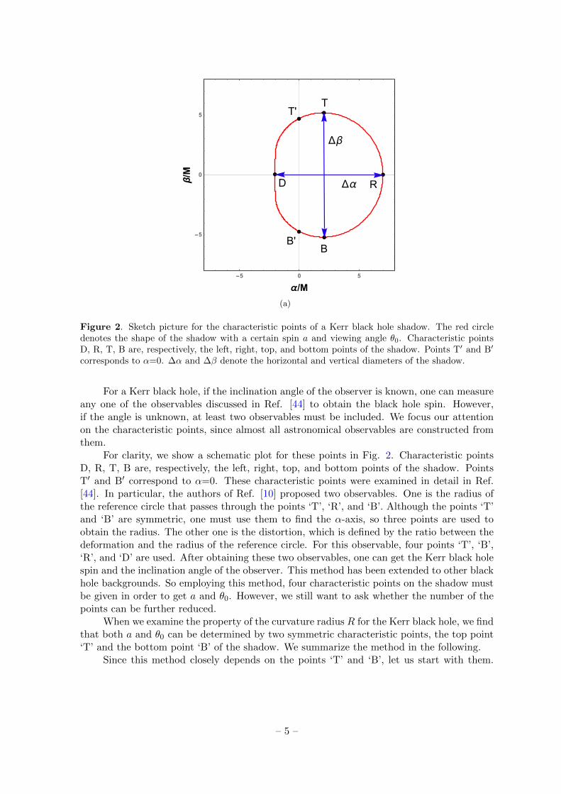
Figure 2. Sketch picture for the characteristic points of a Kerr black hole shadow. The red circledenotes the shape of the shadow with a certain spin a and viewing angle θ0. Characteristic pointsD, R, T, B are, respectively, the left, right, top, and bottom points of the shadow. Points T′ and B′
corresponds to α=0. ∆α and ∆β denote the horizontal and vertical diameters of the shadow.
For a Kerr black hole, if the inclination angle of the observer is known, one can measureany one of the observables discussed in Ref. [44] to obtain the black hole spin. However,if the angle is unknown, at least two observables must be included. We focus our attentionon the characteristic points, since almost all astronomical observables are constructed fromthem.
For clarity, we show a schematic plot for these points in Fig. 2. Characteristic pointsD, R, T, B are, respectively, the left, right, top, and bottom points of the shadow. PointsT′ and B′ correspond to α=0. These characteristic points were examined in detail in Ref.[44]. In particular, the authors of Ref. [10] proposed two observables. One is the radius ofthe reference circle that passes through the points ‘T’, ‘R’, and ‘B’. Although the points ‘T’and ‘B’ are symmetric, one must use them to find the α-axis, so three points are used toobtain the radius. The other one is the distortion, which is defined by the ratio between thedeformation and the radius of the reference circle. For this observable, four points ‘T’, ‘B’,‘R’, and ‘D’ are used. After obtaining these two observables, one can get the Kerr black holespin and the inclination angle of the observer. This method has been extended to other blackhole backgrounds. So employing this method, four characteristic points on the shadow mustbe given in order to get a and θ0. However, we still want to ask whether the number of thepoints can be further reduced.
When we examine the property of the curvature radius R for the Kerr black hole, we findthat both a and θ0 can be determined by two symmetric characteristic points, the top point‘T’ and the bottom point ‘B’ of the shadow. We summarize the method in the following.
Since this method closely depends on the points ‘T’ and ‘B’, let us start with them.
– 5 –
The points are determined by
(∂αβ)a,θ0 = 0. (3.1)
Adopting the parametric forms of α and β, the condition will be reduced to
(∂r0α)−1a,θ0 = 0, (3.2)
or,
(∂r0β)a,θ0 = 0. (3.3)
The first condition (3.2) gives
a(M − r)2 sin θ0 = 0. (3.4)
For θ0 6= 0, one has r = M , which is smaller than the radius of the event horizon of anon-extremal black hole, and thus we turn to another condition. The second condition (3.3)gives
r30 − 3Mr20 + 3M2r0 − a2M = 0, (3.5)
or,
r30 − 3Mr20 + a2 cos2 θ0r0 + a2M cos2 θ0 = 0. (3.6)
Equation (3.5) gives a real root r0 = M −(M3 −Ma2
) 13 , which is also smaller than the
radius of the event horizon, so we abandon it. Finally, by solving Eq. (3.6), we obtain
r0 = M +2√3
√3M2 − a2 cos2 θ0 cos
(1
3arccos
(3√
3M(M2 − a2 cos2 θ20)
(3M2 − a2 cos2 θ0)3/2
)). (3.7)
Inserting this result into (α, β), one will obtain the coordinates (αT , βT ) of the point ‘T’.The result is complicated and we will not show the expression. But from it we can extractthe vertical diameter ∆β of the shadow
∆β = 2βT, (3.8)
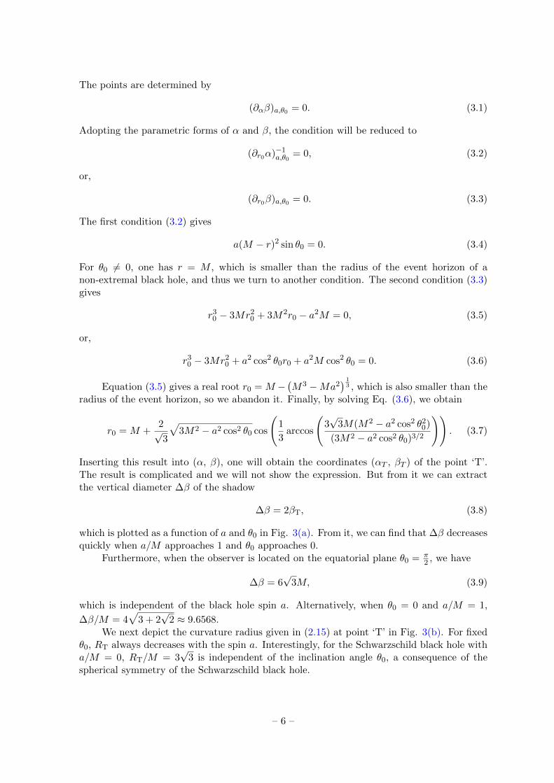
which is plotted as a function of a and θ0 in Fig. 3(a). From it, we can find that ∆β decreasesquickly when a/M approaches 1 and θ0 approaches 0.
Furthermore, when the observer is located on the equatorial plane θ0 = π2 , we have
∆β = 6√
3M, (3.9)
which is independent of the black hole spin a. Alternatively, when θ0 = 0 and a/M = 1,
∆β/M = 4√
3 + 2√
2 ≈ 9.6568.We next depict the curvature radius given in (2.15) at point ‘T’ in Fig. 3(b). For fixed
θ0, RT always decreases with the spin a. Interestingly, for the Schwarzschild black hole witha/M = 0, RT/M = 3
√3 is independent of the inclination angle θ0, a consequence of the
spherical symmetry of the Schwarzschild black hole.
– 6 –
(a)
(b)
Figure 3. (a) The behavior of the vertical diameter ∆β of the shadow as a function of a and θ0. (b)The curvature radius RT of top point ‘T’ as a function of a and θ0.
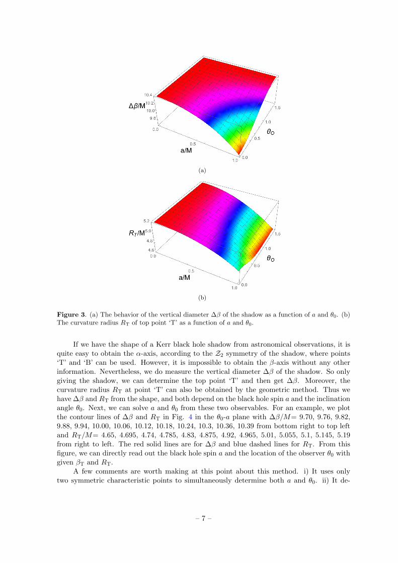
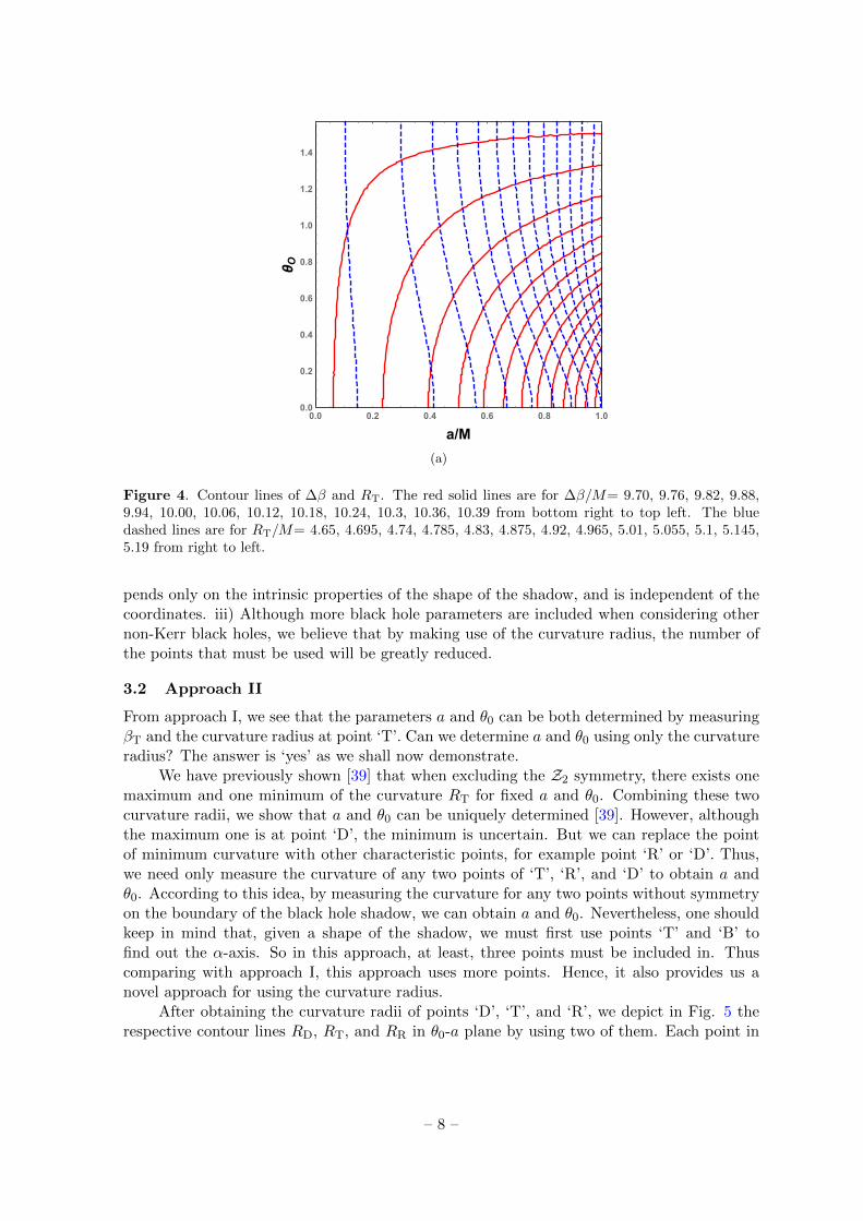
If we have the shape of a Kerr black hole shadow from astronomical observations, it isquite easy to obtain the α-axis, according to the Z2 symmetry of the shadow, where points‘T’ and ‘B’ can be used. However, it is impossible to obtain the β-axis without any otherinformation. Nevertheless, we do measure the vertical diameter ∆β of the shadow. So onlygiving the shadow, we can determine the top point ‘T’ and then get ∆β. Moreover, thecurvature radius RT at point ‘T’ can also be obtained by the geometric method. Thus wehave ∆β and RT from the shape, and both depend on the black hole spin a and the inclinationangle θ0. Next, we can solve a and θ0 from these two observables. For an example, we plotthe contour lines of ∆β and RT in Fig. 4 in the θ0-a plane with ∆β/M= 9.70, 9.76, 9.82,9.88, 9.94, 10.00, 10.06, 10.12, 10.18, 10.24, 10.3, 10.36, 10.39 from bottom right to top leftand RT/M= 4.65, 4.695, 4.74, 4.785, 4.83, 4.875, 4.92, 4.965, 5.01, 5.055, 5.1, 5.145, 5.19from right to left. The red solid lines are for ∆β and blue dashed lines for RT. From thisfigure, we can directly read out the black hole spin a and the location of the observer θ0 withgiven βT and RT.
A few comments are worth making at this point about this method. i) It uses onlytwo symmetric characteristic points to simultaneously determine both a and θ0. ii) It de-
– 7 –
0.0 0.2 0.4 0.6 0.8 1.00.0
0.2
0.4
0.6
0.8
1.0
1.2
1.4
a/M
θO
(a)
Figure 4. Contour lines of ∆β and RT. The red solid lines are for ∆β/M= 9.70, 9.76, 9.82, 9.88,9.94, 10.00, 10.06, 10.12, 10.18, 10.24, 10.3, 10.36, 10.39 from bottom right to top left. The bluedashed lines are for RT/M= 4.65, 4.695, 4.74, 4.785, 4.83, 4.875, 4.92, 4.965, 5.01, 5.055, 5.1, 5.145,5.19 from right to left.
pends only on the intrinsic properties of the shape of the shadow, and is independent of thecoordinates. iii) Although more black hole parameters are included when considering othernon-Kerr black holes, we believe that by making use of the curvature radius, the number ofthe points that must be used will be greatly reduced.
3.2 Approach II
From approach I, we see that the parameters a and θ0 can be both determined by measuringβT and the curvature radius at point ‘T’. Can we determine a and θ0 using only the curvatureradius? The answer is ‘yes’ as we shall now demonstrate.
We have previously shown [39] that when excluding the Z2 symmetry, there exists onemaximum and one minimum of the curvature RT for fixed a and θ0. Combining these twocurvature radii, we show that a and θ0 can be uniquely determined [39]. However, althoughthe maximum one is at point ‘D’, the minimum is uncertain. But we can replace the pointof minimum curvature with other characteristic points, for example point ‘R’ or ‘D’. Thus,we need only measure the curvature of any two points of ‘T’, ‘R’, and ‘D’ to obtain a andθ0. According to this idea, by measuring the curvature for any two points without symmetryon the boundary of the black hole shadow, we can obtain a and θ0. Nevertheless, one shouldkeep in mind that, given a shape of the shadow, we must first use points ‘T’ and ‘B’ tofind out the α-axis. So in this approach, at least, three points must be included in. Thuscomparing with approach I, this approach uses more points. Hence, it also provides us anovel approach for using the curvature radius.
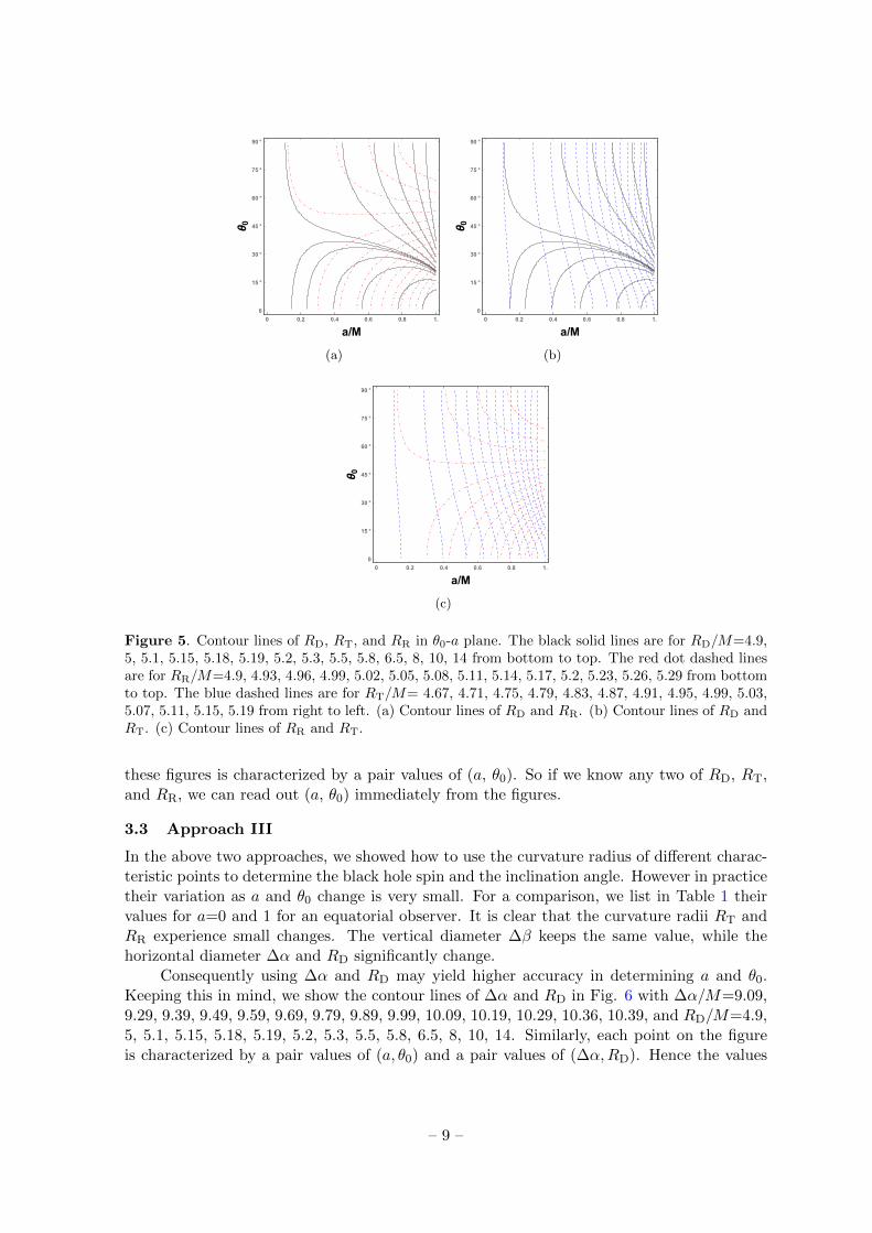
After obtaining the curvature radii of points ‘D’, ‘T’, and ‘R’, we depict in Fig. 5 therespective contour lines RD, RT, and RR in θ0-a plane by using two of them. Each point in
– 8 –
0 0.2 0.4 0.6 0.8 1.
0
15 °
30 °
45 °
60 °
75 °
90 °
a/M
θ0
(a)
0 0.2 0.4 0.6 0.8 1.
0
15 °
30 °
45 °
60 °
75 °
90 °
a/M
θ0
(b)
0 0.2 0.4 0.6 0.8 1.
0
15 °
30 °
45 °
60 °
75 °
90 °
a/M
θ0
(c)
Figure 5. Contour lines of RD, RT, and RR in θ0-a plane. The black solid lines are for RD/M=4.9,5, 5.1, 5.15, 5.18, 5.19, 5.2, 5.3, 5.5, 5.8, 6.5, 8, 10, 14 from bottom to top. The red dot dashed linesare for RR/M=4.9, 4.93, 4.96, 4.99, 5.02, 5.05, 5.08, 5.11, 5.14, 5.17, 5.2, 5.23, 5.26, 5.29 from bottomto top. The blue dashed lines are for RT/M= 4.67, 4.71, 4.75, 4.79, 4.83, 4.87, 4.91, 4.95, 4.99, 5.03,5.07, 5.11, 5.15, 5.19 from right to left. (a) Contour lines of RD and RR. (b) Contour lines of RD andRT. (c) Contour lines of RR and RT.
these figures is characterized by a pair values of (a, θ0). So if we know any two of RD, RT,and RR, we can read out (a, θ0) immediately from the figures.
3.3 Approach III
In the above two approaches, we showed how to use the curvature radius of different charac-teristic points to determine the black hole spin and the inclination angle. However in practicetheir variation as a and θ0 change is very small. For a comparison, we list in Table 1 theirvalues for a=0 and 1 for an equatorial observer. It is clear that the curvature radii RT andRR experience small changes. The vertical diameter ∆β keeps the same value, while thehorizontal diameter ∆α and RD significantly change.
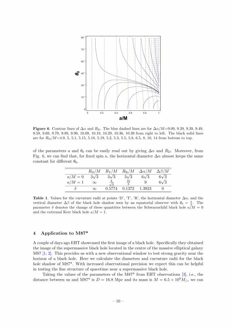
Consequently using ∆α and RD may yield higher accuracy in determining a and θ0.Keeping this in mind, we show the contour lines of ∆α and RD in Fig. 6 with ∆α/M=9.09,9.29, 9.39, 9.49, 9.59, 9.69, 9.79, 9.89, 9.99, 10.09, 10.19, 10.29, 10.36, 10.39, and RD/M=4.9,5, 5.1, 5.15, 5.18, 5.19, 5.2, 5.3, 5.5, 5.8, 6.5, 8, 10, 14. Similarly, each point on the figureis characterized by a pair values of (a, θ0) and a pair values of (∆α,RD). Hence the values
– 9 –
0 0.2 0.4 0.6 0.8 1.
0
15 °
30 °
45 °
60 °
75 °
90 °
a/M
θ0
Figure 6. Contour lines of ∆α and RD. The blue dashed lines are for ∆α/M=9.09, 9.29, 9.39, 9.49,9.59, 9.69, 9.79, 9.89, 9.99, 10.09, 10.19, 10.29, 10.36, 10.39 from right to left. The black solid linesare for RD/M=4.9, 5, 5.1, 5.15, 5.18, 5.19, 5.2, 5.3, 5.5, 5.8, 6.5, 8, 10, 14 from bottom to top.
of the parameters a and θ0 can be easily read out by giving ∆α and RD. Moreover, fromFig. 6, we can find that, for fixed spin a, the horizontal diameter ∆α almost keeps the sameconstant for different θ0.
RD/M RT/M RR/M ∆α/M ∆β/M
a/M = 0 3√
3 3√
3 3√
3 6√
3 6√
3
a/M = 1 ∞ 8√3
163 9 6
√3
δ ∞ 0.5774 0.1372 1.3923 0
Table 1. Values for the curvature radii at points ‘D’, ‘T’, ‘R’, the horizontal diameter ∆α, and thevertical diameter ∆β of the black hole shadow seen by an equatorial observer with θ0 = π
2 . Theparameter δ denotes the change of these quantities between the Schwarzschild black hole a/M = 0and the extremal Kerr black hole a/M = 1.
4 Application to M87*
A couple of days ago EHT showcased the first image of a black hole. Specifically they obtainedthe image of the supermassive black hole located in the centre of the massive elliptical galaxyM87 [1, 2]. This provides us with a new observational window to test strong gravity near thehorizon of a black hole. Here we calculate the diameters and curvature radii for the blackhole shadow of M87*. With increased observational precision we expect this can be helpfulin testing the fine structure of spacetime near a supermassive black hole.
Taking the values of the parameters of the M87* from EHT observations [3], i.e., thedistance between us and M87* is D = 16.8 Mpc and its mass is M = 6.5 × 10⁹M�, we can
– 10 –
calculate the gravitational radius [3]
θg =GM
c2D≈ 3.8 µas . (4.1)
Since the approaching jet and the line of sight is 16◦ [48], we only focus our attention onthe viewing angle θ0 around 16◦. Moreover, adopting the Standard and Normal Evolution(SANE) and Magnetically Arrested Disk (MAD) models, one can find from the rejectiontable of [2] that the black hole spin |a|=0.5 and 0.94 can pass these different constraints.Thus we consider values of a within this range in our calculation.
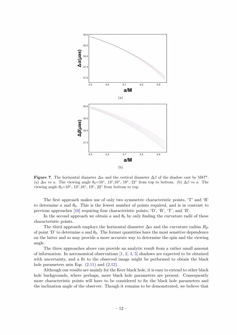
We show the horizontal and vertical diameters of the black hole shadow cast by M87*in Fig. 7 with varying the viewing angle θ0=10◦, 13◦,16◦, 19◦, 22◦, respectively. For fixedθ0, both the diameters ∆α and ∆β decrease with the black hole spin. For fixed black holespin a, ∆α decreases whereas ∆β increases with increasing θ0. At a = 0.5, both ∆α and∆β are near 38.9 µas. When a increases to 0.94, the vertical diameter ∆β is about 37.3µas. The horizontal diameter ∆α can even approach 37 µas. Thus the shape of the shadowwill be increasingly deformed for high spin. Moreover, for low spin, ∆α and ∆β are almostindependent of the viewing angle θ0.
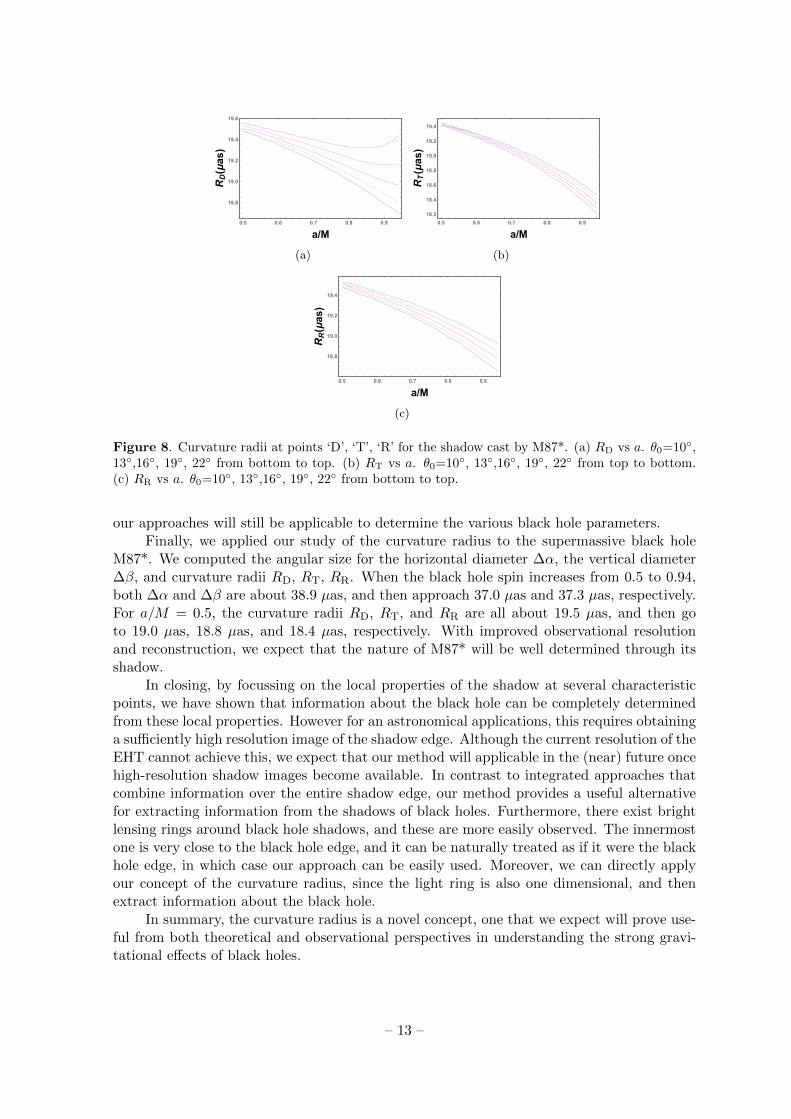
The curvature radii at points ‘D’, ‘T’, ‘R’ are each plotted against the black hole spin inFig. 8 for θ0=10◦, 13◦,16◦, 19◦, and 22◦. For small viewing angle θ0, RD decreases with theblack hole spin. However for θ0 larger than 13◦, e.g., θ0 = 22◦, RD first decreases from about19.6 µas to 19.3 µas and then increases to 19.4 µas with increasing a. Thus, if θ0 > 13◦ wecannot determine the black hole spin even if RD is known, unless some other conditions areconsidered. Meanwhile, when a varies from 0.5 to 0.94, RT decreases from 19.4 µas to 18.2µas, and RR decreases from 19.5 µas to 18.7 µas.
a/M 0.5 0.6 0.7 0.8 0.9 0.94
∆α(µas) 38.91 38.64 38.29 37.85 37.28 37.00∆β(µas) 38.96 38.71 38.40 38.03 37.56 37.34RD(µas) 19.51 19.40 19.28 19.14 19.01 18.97RT(µas) 19.50 19.39 19.25 19.08 18.87 18.78RR(µas) 19.43 19.28 19.09 18.84 18.51 18.35
Table 2. Angular size of the quantities for the shadow cast by M87* with viewing angle θ0 = 16◦.
For comparison, we list the values of these quantities ∆α, ∆β, RD, RT, and RR in Table2 when θ0 = 16◦ is fixed. For two small values of the spin, the differences between them arevery tiny. However, for two high spins a/M=0.7 and 0.94, the differences of ∆α, ∆β, RD,RT, and RR between them are, respectively, about 1.3, 1.1, 0.3, 0.5, and 0.7 µas. Thus, whenthe precision of EHT is improved to around 1 µas comparing with current resolution 5 µas inthe final reconstructed images, the black hole spin can be well determined in high spin case.
5 Conclusions and discussions
In this paper, we mainly considered the application of the curvature radius we previouslyproposed [39]. Based on the characteristic points and making use of the curvature radius, wehave put forward three novel approaches to determine the spin of the Kerr black hole andthe inclination angle of the observer.
– 11 –
0.5 0.6 0.7 0.8 0.9
37.0
37.5
38.0
38.5
39.0
a/M
Δα(μas
)
(a)
0.5 0.6 0.7 0.8 0.9
37.5
38.0
38.5
39.0
a/M
Δβ(μas
)
(b)
Figure 7. The horizontal diameter ∆α and the vertical diameter ∆β of the shadow cast by M87*.(a) ∆α vs a. The viewing angle θ0=10◦, 13◦,16◦, 19◦, 22◦ from top to bottom. (b) ∆β vs a. Theviewing angle θ0=10◦, 13◦,16◦, 19◦, 22◦ from bottom to top.
The first approach makes use of only two symmetric characteristic points, ‘T’ and ‘B’to determine a and θ0. This is the fewest number of points required, and is in contrast toprevious approaches [10] requiring four characteristic points, ‘D’, ‘R’, ‘T’, and ‘B’.
In the second approach we obtain a and θ0 by only finding the curvature radii of thesecharacteristic points.
The third approach employs the horizontal diameter ∆α and the curvature radius RD
of point ‘D’ to determine a and θ0. The former quantities have the most sensitive dependenceon the latter and so may provide a more accurate way to determine the spin and the viewingangle.
The three approaches above can provide an analytic result from a rather small amountof information. In astronomical observations [1, 2, 4, 5] shadows are expected to be obtainedwith uncertainty, and a fit to the observed image might be performed to obtain the blackhole parameters usin Eqs. (2.11) and (2.12).
Although our results are mainly for the Kerr black hole, it is easy to extend to other blackhole backgrounds, where perhaps, more black hole parameters are present. Consequentlymore characteristic points will have to be considered to fix the black hole parameters andthe inclination angle of the observer. Though it remains to be demonstrated, we believe that
– 12 –
0.5 0.6 0.7 0.8 0.9
18.8
19.0
19.2
19.4
19.6
a/M
RD(μas
)
(a)
0.5 0.6 0.7 0.8 0.9
18.2
18.4
18.6
18.8
19.0
19.2
19.4
a/M
RT(μas
)
(b)
0.5 0.6 0.7 0.8 0.9
18.8
19.0
19.2
19.4
a/M
RR(μas
)
(c)
Figure 8. Curvature radii at points ‘D’, ‘T’, ‘R’ for the shadow cast by M87*. (a) RD vs a. θ0=10◦,13◦,16◦, 19◦, 22◦ from bottom to top. (b) RT vs a. θ0=10◦, 13◦,16◦, 19◦, 22◦ from top to bottom.(c) RR vs a. θ0=10◦, 13◦,16◦, 19◦, 22◦ from bottom to top.
our approaches will still be applicable to determine the various black hole parameters.Finally, we applied our study of the curvature radius to the supermassive black hole
M87*. We computed the angular size for the horizontal diameter ∆α, the vertical diameter∆β, and curvature radii RD, RT, RR. When the black hole spin increases from 0.5 to 0.94,both ∆α and ∆β are about 38.9 µas, and then approach 37.0 µas and 37.3 µas, respectively.For a/M = 0.5, the curvature radii RD, RT, and RR are all about 19.5 µas, and then goto 19.0 µas, 18.8 µas, and 18.4 µas, respectively. With improved observational resolutionand reconstruction, we expect that the nature of M87* will be well determined through itsshadow.
In closing, by focussing on the local properties of the shadow at several characteristicpoints, we have shown that information about the black hole can be completely determinedfrom these local properties. However for an astronomical applications, this requires obtaininga sufficiently high resolution image of the shadow edge. Although the current resolution of theEHT cannot achieve this, we expect that our method will applicable in the (near) future oncehigh-resolution shadow images become available. In contrast to integrated approaches thatcombine information over the entire shadow edge, our method provides a useful alternativefor extracting information from the shadows of black holes. Furthermore, there exist brightlensing rings around black hole shadows, and these are more easily observed. The innermostone is very close to the black hole edge, and it can be naturally treated as if it were the blackhole edge, in which case our approach can be easily used. Moreover, we can directly applyour concept of the curvature radius, since the light ring is also one dimensional, and thenextract information about the black hole.
In summary, the curvature radius is a novel concept, one that we expect will prove use-ful from both theoretical and observational perspectives in understanding the strong gravi-tational effects of black holes.
– 13 –
Acknowledgements
This work was supported by the National Natural Science Foundation of China (Grants Nos.11675064, 11875151, 11522541, and U1738132) and the Natural Sciences and EngineeringResearch Council of Canada. S.-W. Wei was also supported by the Chinese ScholarshipCouncil (CSC) Scholarship (201806185016) to visit the University of Waterloo.
References
[1] The Event Horizon Telescope Collaboration, First M87 Event Horizon Telescope Results. I.The Shadow of the Supermassive Black Hole, Astrophys. J. Lett. 875, L1 (2019).
[2] The Event Horizon Telescope Collaboration, First M87 Event Horizon Telescope Results. V.Physical Origin of the Asymmetric Ring, Astrophys. J. Lett. 875, L5 (2019).
[3] The Event Horizon Telescope Collaboration, First M87 Event Horizon Telescope Results. VI.The Shadow and Mass of the Central Black Hole, Astrophys. J. Lett. 875, L6 (2019).
[4] A. M. Hughes, A. Beasley, and C. Carilli , Next Generation Very Large Array: CentimeterRadio Astronomy in the 2020s, IAU General Assembly, 22, 2255106 (2015).
[5] G. H. Sanders, The Thirty Meter Telescope (TMT): An International Observatory, Journal ofAstrophysics and Astronomy, 34, 81 (2013).
[6] J. L. Synge, The escape of photons from gravitationally intense stars, MNRAS, 131, 463 (1966).
[7] J. P. Luminet, Image of a spherical black hole with thin accretion disk, A. A, 75, 228 (1979).
[8] J. M. Bardeen, Timelike and null geodesics in the Kerr metric, Les Astres Occlus, (1973).
[9] S. Chandrasekhar, The Mathematical Theory of Black Holes, Oxford University Press, NewYork, (1992).
[10] K. Hioki and K. I. Maeda, Measurement of the Kerr Spin Parameter by Observation of aCompact Object’s Shadow, Phys. Rev. D 80, 024042 (2009), [arXiv:0904.3575 [astro-ph.HE]].
[11] T. Johannsen, Photon rings around Kerr and Kerr-like black holes, Astrophys. J. 777, 170(2013), [arXiv:1501.02814 [astro-ph.HE]].
[12] M. Ghasemi-Nodehi, Z.-L. Li, and C. Bambi, Shadows of CPR black holes and tests of the Kerrmetric, Eur. Phys. J. C 75, 315 (2015), [arXiv:1506.02627 [gr-qc]].
[13] C. Bambi and K. Freese, Apparent shape of super-spinning black holes, Phys. Rev. D 79,043002 (2009), [arXiv:0812.1328 [astro-ph]];
[14] L. Amarilla, E. F. Eiroa, and G. Giribet, Null geodesics and shadow of a rotating black hole inextended Chern-Simons modified gravity, Phys. Rev. D 81, 124045 (2010), [arXiv:1005.0607[gr-qc]].
[15] Z. Stuchlik and J. Schee, Appearance of Keplerian discs orbiting Kerr superspinars, Class.Quant. Grav. 27, 215017 (2010), [arXiv:1101.3569 [gr-qc]].
[16] L. Amarilla and E. F. Eiroa, Shadow of a Kaluza-Klein rotating dilaton black hole, Phys. Rev.D 87, 044057 (2013), [arXiv:1301.0532 [gr-qc]].
[17] P. G. Nedkova, V. K. Tinchev, and S. S. Yazadjiev, The shadow of a rotating traversablewormhole, Phys. Rev. D 88, 124019, (2013) [arXiv:1307.7647 [gr-qc]].
[18] S.-W. Wei and Y.-X. Liu, Observing the shadow of Einstein-Maxwell-Dilaton-Axion black hole,JCAP 1311, 063 (2013), [arXiv:1311.4251 [gr-qc]].
[19] N. Tsukamoto, Z.-L. Li, and C. Bambi, Constraining the spin and the deformation parametersfrom the black hole shadow, JCAP 1406, 043 (2014), [arXiv:1403.0371 [gr-qc]].
– 14 –
[20] C. Bambi and N. Yoshida, Shape and position of the shadow in the δ=2 Tomimatsu-Satospace-time, Class. Quant. Grav. 27, 205006 (2010), [arXiv:1004.3149 [gr-qc]].
[21] F. Atamurotov, A. Abdujabbarov, and B. Ahmedov, Shadow of rotating non-Kerr black hole,Phys. Rev. D 88, 064004 (2013).
[22] S. Abdolrahimi, R. B. Mann, and C. Tzounis, Distorted local shadows, Phys. Rev. D 91,084052 (2015), [arXiv:1502.00073 [gr-qc]].
[23] S.-W. Wei, P. Cheng, Y. Zhong, and X.-N. Zhou, Shadow of noncommutative geometry inspiredblack hole, JCAP 1508, 004 (2015), [arXiv:1501.06298 [gr-qc]].
[24] F. Atamurotov, B. Ahmedov, and A. Abdujabbarov, Optical properties of black hole in thepresence of plasma: shadow, Phys. Rev. D 92, 084005 (2015), [arXiv:1507.08131 [gr-qc]].
[25] A. Abdujabbarov, M. Amir, B. Ahmedov, and S. G. Ghosh, Shadow of rotating regular blackholes, Phys. Rev. D 93, 104004 (2016), [arXiv:1604.03809 [gr-qc]].
[26] M.-Z. Wang, S.-B. Chen, and J.-L. Jing, Shadow casted by a Konoplya-Zhidenko rotatingnon-Kerr black hole, JCAP 1710, 051 (2017), [arXiv:1707.09451 [gr-qc]].
[27] M. Amir, B. P. Singh, and S. G. Ghosh, Shadows of rotating five-dimensional charged EMCSblack holes, Eur. Phys. J. C 78, 399 (2018), [arXiv:1707.09521 [gr-qc]].
[28] N. Tsukamoto, Black hole shadow in an asymptotically-flat, stationary, and axisymmetricspacetime: The Kerr-Newman and rotating regular black holes, Phys. Rev. D 97, 064021(2018), [arXiv:1708.07427 [gr-qc]].
[29] M.-Z. Wang, S.-B. Chen, and J.-L. Jing, Shadows of Bonnor black dihole by chaotic lensing,Phys. Rev. D 97, 064029 (2018), [arXiv:1710.07172 [gr-qc]].
[30] R. Shaikh, Shadows of rotating wormholes, Phys. Rev. D 98, 024044 (2018), [arXiv:1803.11422[gr-qc]].
[31] X. Hou, Z.-Y. Xu, M. Zhou, and J.-C. Wang, Black hole shadow of Sgr A∗ in dark matter halo,JCAP 1807, 015 (2018), [arXiv:1804.08110 [gr-qc]].
[32] P. V. P. Cunha, C. A. R. Herdeiro, E. Radu, and H. F. Runarsson, Shadows of Kerr black holeswith scalar hair, Phys. Rev. Lett. 115, 211102 (2015), [arXiv:1509.00021 [gr-qc]].
[33] P. V. P. Cunha, C. A. R. Herdeiro, and E. Radu, Fundamental photon orbits: black holeshadows and spacetime instabilities, Phys. Rev. D 96, 024039 (2017), [arXiv:1705.05461 [gr-qc]].
[34] P. V. P. Cunha and C. A. R. Herdeiro, Shadows and strong gravitational lensing: a briefreview, Gen. Rel. Grav. 50, 42 (2018), [arXiv:1801.00860 [gr-qc]].
[35] O. Yu. Tsupko, Analytical calculation of black hole spin using deformation of the shadow, Phys.Rev. D 95, 104058 (2017), [arXiv:1702.04005 [gr-qc]].
[36] V. Perlick, O. Yu. Tsupko, and G. S. Bisnovatyi-Kogan, Black hole shadow in an expandinguniverse with a cosmological constant, Phys. Rev. D 97, 104062 (2018), [arXiv:1804.04898[gr-qc]].
[37] R. Shaikh, P. Kocherlakota, R. Narayan, and P. S. Joshi, Shadows of spherically symmetricblack holes and naked singularities, Mon. Not. Roy. Astron. Soc. 482, 52 (2019),[arXiv:1802.08060 [astro-ph.HE]].
[38] H.-M. Wang, Y.-M. Xu, and S.-W. Wei, Shadows of Kerr-like black holes in a modified gravitytheory, JCAP 1903, 046 (2019), [arXiv:1810.12767 [gr-qc]].
[39] S.-W. Wei, Y.-X. Liu, and R. B. Mann, Intrinsic curvature and topology of shadow in Kerrspacetime, Phys. Rev. D 99, 041303(R) (2019), [arXiv:1811.00047 [gr-qc]].
– 15 –
[40] Z. Younsi, A. Zhidenko, L. Rezzolla, R. Konoplya, and Y. Mizuno, New method for shadowcalculations: Application to parametrized axisymmetric black holes, Phys. Rev. D 94, 084025(2016) [arXiv:1607.05767 [gr-qc]].
[41] A. K. Mishra, S. Chakraborty, and S. Sarkar, Understanding photon sphere and black holeshadow in dynamically evolving spacetimes, [arXiv:1903.06376 [gr-qc]].
[42] A. B. Abdikamalov, A. A. Abdujabbarov, D. Malafarina, C. Bambi, and B. Ahmedov, A blackhole mimicker hiding in the shadow: Optical properties of the γ metric, [arXiv:1904.06207[gr-qc]].
[43] A. A. Abdujabbarov, L. Rezzolla, and B. J. Ahmedov, A coordinate-independentcharacterization of a black hole shadow, Mon. Not. Roy. Astron. Soc. 454, 2423 (2015),[arXiv:1503.09054 [gr-qc]].
[44] S.-W. Wei and Y.-X. Liu, Parametric study of Kerr black hole shadow: analytical and exactcalculations, in preparation, (2019).
[45] K. Yano, Some remarks on tensor fields and curvature, Ann. Math. 55, 328 (1952).
[46] R. Penrose, Naked singularities, Ann. N. Y. Acad. Sci. 224, 125 (1973).
[47] P. J. Young, Capture of particles from plunge orbits by a black hole, Phys. Rev. D 14, 3281(1976).
[48] R. C. Walker, P. E. Hardee, F. B. Davies, C. Ly, and W. Junor, The Structure and Dynamicsof the Sub-parsec Scale Jet in M87 Based on 50 VLBA Observations Over 17 Years at 43 GHz,Astrophys. J. 855, 128 (2018), [arXiv:1802.06166 [astro-ph.HE]].
– 16 –