Cursed Equilibrium

Erik EysterNuffield College, Oxford

and

Matthew RabinDepartment of Economics

University of California, Berkeley

November 1, 2000

Abstract

There is evidence that people do not fully take into account how other peoplesactions are contingent on these others information. This paper deÞnes and appliesa new equilibrium concept in games with private information, cursed equilibrium,which assumes that each player correctly predicts the distribution of other playersactions, but underestimates the degree to which these actions are correlated withthese other players information. We apply the concept to common-values auc-tions, where cursed equilibrium captures the widely-observed phenomenon of thewinners curse. We also show how cursed equilibrium predicts other empirically-observed phenomena, such as trade in adverse-selection settings where conven-tional analysis predicts no trade, and naive voting in elections and juries whererational-choice models predict that voters fully take into account the informationalcontent in being pivotal.

Keywords: Curses!

JEL ClassiÞcations: B49

Acknowledgments: We thank Colin Camerer and seminar participants at Berkeley,Cal Tech, and Nuffield College (Oxford) for helpful comments, and Davis Beek-man, Kitt Carpenter, and David Huffman for valuable research assistance. Eysterthanks the Olin and MacArthur Foundations, and Rabin thanks the Russell Sage,Sloan, MacArthur, and National Science Foundations for Þnancial support. Bothauthors deny using cocaine less than 26 years before working on this paper.

Contacts: E-mail: erik.eyster@nuffield.oxford.ac.uk and rabin@econ.berkeley.edu.Rabins web page: <http://elsa.berkeley.edu/rabin/index.html>.

1 Introduction

A widely observed phenomenon in laboratory auctions is the winners curse: when bidders

who share a common but unknown value for a good have private information about the

goods value, they tend to bid more than equilibrium theory predicts. In many experiments,

the average winning bid exceeds the average value of the good. One explanation for this

phenomenon is that the typical bidder fails to fully appreciate that the low bids by other

bidders needed for her to win the auction mean that these other bidders private information is

more negative than her own. This failure leads the bidder to believe that the value of the object

when she wins the auction is closer to the value suggested by her private information than

it actually is, and hence to overbid. Fully rational bidders avoid this problem by tempering

their bids.

While the winners curse has been observed repeatedly in laboratory experiments, and

anecdotes and some research suggests that it is important outside of the laboratory, theo-

retical research on auctions assumes that people do not make this error.1 Indeed, empirical

researchers base their estimations of bidders valuations for the object being auctioned on the

presumption that bidders do not make this error.2 Kagel and Levin (1986) and others in

the context of common-values auctions, as well as Holt and Sherman (1994) in the context of

trade with adverse selection, have posited and tested an extreme form of the winners curse:

agents act as if there is no information content in winning an auction or completing a trade.3

In this paper, we formally model a generalization of the winners curse which assumes that

players in a Bayesian game underestimate the extent to which other players actions are cor-

related with their information. Our model generalizes those of Kagel and Levin (1988) and

Holt and Sherman (1994) both by allowing players to partially, but not fully, appreciate the

information content in other players actions, and by deÞning a solution concept applicable

to general Bayesian games. We ßesh out the implications of our model in common-values

auctions and many other settings, discussing the empirical evidence that motivates it in the

1See Thaler (1988) for an overview of the early evidence on the winners curse as well as Kagel (1995) fora survey of laboratory auctions.

2 In fact, when winners curse appears in the title of a paper, it typically refers to the study of playerswho avoid rather than succumb to the curse. Just as suburban housing developments are often named afterthe bit of nature obliterated to create them (Forest Glen), so too the term winners curse is typically usedto describe what isnt there.

3Potters and Wit (1995) and Jacobsen, Potters, Schram, van Winden, and Wit (2000) use this same premiseanalyze markets for assets whose values are common but unknown to the traders.

1

speciÞc contexts we consider. The model ties together a wide range of empirically observed

phenomena with a formalization of a single psychological principle the underappreciation

of the informational content of the behavior of others.

In Section 2 we present our equilibrium concept. We consider standard Bayesian games

where players private information is represented by their types, whose joint distribution is

common knowledge. Our equilibrium concept, cursed equilibrium, assumes that each player

incorrectly believes that with positive probability each proÞle of types of the other players

plays the average action of what all types of other players are playing, rather than their true,

type-speciÞc action. Players choose their actions to maximize their expected utilities given

their types and these incorrect beliefs about other players equilibrium strategies. We parame-

terize the extent to which a player is cursed by the probability χ ∈ [0, 1] she assigns to otherplayers playing their average action rather than their type-contingent strategy. Setting χ = 0

corresponds to the fully rational Bayesian Nash equilibrium, and setting χ = 1 corresponds to

the case where each player assumes no connection whatsoever between other players actions

and their types. Whatever χ, each player correctly predicts the equilibrium distribution

of the other players actions the players only mistake comes in misunderstanding the

relationship between other players types and their actions.

To illustrate cursed equilibrium, consider a simple variant of Akerlofs (1970) lemons model

in which a buyer might purchase a car from a seller at a predetermined price of $1, 000. The

seller knows whether the car is a lemon, worth $0 to both the seller and buyer, or a peach,

worth $3, 000 to the buyer and $2, 000 to the seller. The buyer believes each occurs with

probability 12 . The parties simultaneously announce whether they wish to trade, and the car

is sold if and only if both say they wish to trade. While a fully rational buyer would realize

that the seller will sell if and only if the car is a lemon, and hence refuse to buy, a cursed

buyer may mistakenly buy the car. The sure sale of the lemon is a χ-cursed equilibrium

because a χ-cursed buyer believes that with probability χ the seller sells irrespective of the

type of car, so that the car being sold is a peach with probability with (1−χ) · 0+χ · 12 =

χ2 ,

and therefore worth χ2 · 3, 000 = 1, 500χ. Hence, a buyer cursed by χ > 2

3 will buy the car,

only to discover that whenever the seller is willing to sell it is a worthless lemon.

We prove that every Þnite game has (for every value of χ) a cursed equilibrium by

observing that a cursed equilibrium corresponds to a Bayesian Nash equilibrium in a modiÞed

game where the players payoffs for each action and type proÞle are a weighted average of their

2

actual payoffs and their average payoffs for that action proÞle averaged over other players

types. We also show that when each players payoffs are fully independent of other players

types, cursed equilibrium and Bayesian Nash equilibrium coincide. Intuitively, the only

difference between the two equilibrium concepts is that in a cursed equilibrium players have

incorrect beliefs about the relationship between their opponents actions and their types; if no

players payoffs depend on any other players type, then such mistaken beliefs do not matter.

Finally, we deÞne a perfectly-cursed equilibrium, the analogue to Perfect Bayesian equilibrium,

and show how it imposes an important restriction on players beliefs off the equilibrium path.

In Sections 3, 4, and 5, we apply the general model to three different important settings

bilateral trade, auctions, and voting. Our model both helps to explain existing experimental

behavior in these settings and provides plausible, testable predictions in settings for which we

know of no experimental evidence. In Section 3 we examine adverse selection and no-trade

theorems in the context of bilateral trade. When, as in the example above, a seller has

private information about the value of a good, while the buyer does not, cursed equilibrium

may lead to more trade than Bayesian Nash equilibrium: when only sellers with low-value

goods sell, a buyer who fails to recognize this may buy when she would be better off not

buying. But cursed equilibrium may also lead to less trade than Bayesian Nash equilibrium:

because a cursed buyer does not fully appreciate that sellers with high-value goods sell at

high prices, she may be too reluctant to pay higher prices. We show that the predictions of

cursed equilibrium approximately correspond to the behavior of subjects in experimental tests

of a lemons model by Samuelson and Bazerman (1985) and Holt and Sherman (1994). We

also illustrate how in a setting with two-sided private information and common preferences,

both parties may strictly prefer trading to not trading, in contrast to no-trade results such

as those presented in Milgrom and Stokey (1982). This is because a buyer or seller who

underinfers the other partys information conditional on trade may agree to a trade with a

negative expected value.

In Section 4 we turn to our primary motivating application, common-values auctions. In

a cursed equilibrium, bidders in a symmetric equilibrium do not recognize that they win the

auction only when they have the most positive information about the value of the object.

When χ and the number of bidders are high enough, this leads to the winners curse the

average winning bid exceeds the average value of the object. Even though cursed bidders may

suffer the winners curse, while rational bidders never do, we show that cursedness does not

3

always raise the sellers expected revenue, because cursed bidders may also sometimes bid less

than rational bidders. Finally, we compare the predictions of cursed equilibrium to some of

the experimental evidence on common-values auctions.

In Section 5 we apply cursed equilibrium to a model of voting, contrasting our predictions

to those of a recent rational-choice literature on voting in elections and on juries. This

literature assumes that people vote with a sophisticated understanding that they should

predicate their votes on being pivotal, which means a voter should vote not based on her

beliefs at the time of voting, but rather based on what her beliefs would be if her vote decided

the election. Just as in bidding, therefore, voters must predict the relationship between other

voters private information and their votes. We show that because of this underinference,

cursed voters are more likely to vote naively according to their beliefs at the time of voting.

This, in turn, implies that in contrast to the rational-choice literature, voting rules in large

elections matter in a cursed equilibrium: whereas uncursed voters adjust their behavior to the

voting rule to assure the efficient outcome, sufficiently cursed voters do not react to voting

rules, so that rules are efficient if and only if they implement the right outcome when voters

vote naively. We also discuss whether cursed equilibrium can help explain McKelvey and

Palfreys (1998) Þndings in their experimental test of jury voting.

In Section 6, we illustrate the implications of cursed equilibrium in two different signaling

contexts. First, we consider classical simple signaling games, where fully-cursed equilibrium

rules out the use of costly signaling, but lesser degrees of cursedness can either destroy mean-

ingful signaling arising in a Bayesian Nash equilibrium or facilitate meaningful signaling that

could not arise in a Bayesian Nash equilibrium. Second, we apply cursed equilibrium to a

model of veriÞable cheap talk modeled after American political elections where voters make

inferences about candidates after these candidates strategically reveal or conceal information

about their past indiscretions or future plans. In this game, one Bayesian Nash equilibrium

is for each type of politician to reveal her type, since any politician who knows the truth

to be less damaging than fully rational voters infer from silence prefers to reveal. Because

cursed voters may not infer the worst from silence they may believe that even good

types conceal even politicians with not-so-bad information may not reveal the truth.

Because it posits that each player correctly predicts the equilibrium distribution of other

players actions without correctly predicting their type-contingent strategies, cursed equilib-

rium is incompatible with many natural explanations for how equilibrium play arises. In

4

some settings, however, we think this is a natural occurrence: a player who observes repeated

play of a single game may learn the distribution of other players actions, but because she may

never observe other players private information she may not learn the relationship between

the other players actions and private information. While we do not Þnd this foundation for

our approach fully satisfying, we believe cursed equilibrium provides a useful, general, and

relatively non-arbitrary way to study the behavioral implications of a pervasive form of failure

of contingent thinking.

Our formulation of cursed equilibrium is an over-simpliÞcation in many other ways that

may limit its applicability beyond the set of games we consider. In some contexts, our

formulation may make some unrealistic predictions; in others, cursed equilibrium is not well-

deÞned. We conclude the paper in Section 7 with a discussion of possible extensions of the

notion of cursed equilibrium that might cope with these problems, as well as discussing some

possible further economic applications of the principles developed in this paper.

2 Definition and General Results

Before developing speciÞc applications, in this section we formally deÞne cursed equilibrium,

prove its existence in all Þnite Bayesian games, and develop some general principles and re-

sults. Consider a Þnite Bayesian Game, G = (A1, . . ., AN ;T0, T1, . . ., TN ; p;u1, . . ., uN ), played

by players k ∈ 1, ...,N. Ak is the Þnite set of Player ks actions, where in a sequential gamean action speciÞes what Player k does at each of her information sets; Tk is the Þnite set of

Player ks types, each type representing different information that Player k can have. For

conceptual and notational ease in our analysis below, we include a set of natures types,

T0. T ≡ T0 × T1 × ... × TN is the set of type proÞles, and p is the probability distribution

over T , which we assume is common to all players. Player ks payoff function uk : A× T → R

depends on all players actions A ≡ A1× ...×AN and their types. A (mixed) strategy σk forPlayer k speciÞes a probability distribution over actions for each type: σk : Tk → 4Ak. Letσk(ak|tk) be the probability that type tk plays action ak, and let u ≡ (u1, ..., uN ).

The common prior probability distribution p puts positive weight on each tk ∈ Tk, and pfully determines the probability distributions pk(t−k|tk), Player ks conditional beliefs aboutthe types T−k ≡ ×

j 6=kTj of other players (including nature) given her own type tk ∈ Tk. Let

5

A−k ≡ ×j 6=0,k

Aj be the set of action proÞles for players j 6= k (excluding nature, who takes noaction), and σ−k : T−k → ×

j 6=0,k4Aj be a strategy of Player ks opponents, where σ−k(a−k|t−k)

is the probability that type t−k ∈ T−k plays action proÞle a−k under strategy σ−k(t−k).The standard solution concept in such games is Bayesian Nash equilibrium:

Definition 1 A strategy proÞle σ is a Bayesian Nash equilibrium if for each Player k, each

type tk ∈ Tk, and each a∗k such that σk(a∗k|tk) > 0,

a∗k ∈ arg maxak∈Ak

Xt−k∈T−k

pk(t−k|tk) ·X

a−k∈A−kσ−k(a−k|t−k)uk(ak, a−k; tk, t−k).

In a Bayesian Nash equilibrium, each player correctly predicts both the probability distribu-

tion over the other players actions and the correlation between the other players actions and

types.

Before deÞning cursed equilibrium, we deÞne for each type of each player the average

strategy of other players, averaged over the other players types. Formally, for all tk ∈ Tk,deÞne σ−k(·|tk) by

σ−k(a−k|tk) ≡X

t−k∈T−kpk(t−k|tk) · σ−k(a−k|t−k).

When Player k is of type tk, σ−k(a−k|tk) is the probability that players j 6= k play action

proÞle a−k when they follow strategy σ−k. A player who (mistakenly) believes that each type

proÞle of the other players plays the same mixed action proÞle believes that the other players

are playing σ−k(·|tk) whenever they play σ−k(a−k|t−k). Note that σ−k(a−k|tk) depends ontk, so different types of Player k have different beliefs about the average action of players

j 6= k. Let σ−k(tk) : T−k → ×j 6=0,k

4Aj denote tks beliefs about the average strategy ofplayers j 6= k, namely σ−k(tk) is the strategy players j 6= k would play if each type proÞle

t−k played a−k with probability σ−k(a−k|tk).From this, we deÞne a cursed equilibrium, deÞned with respect to a parameter χ ∈ [0, 1]

that measures the degree to which players misperceive the correlation between their oppo-

nents actions and types:

Definition 2 A mixed-strategy proÞle σ is a χ-cursed equilibrium if for each k, tk ∈ Tk, andeach a∗k such that σk(a

∗k|tk) > 0,

a∗k ∈ arg maxak∈Ak

Xt−k∈T−k

pk(t−k|tk)·X

a−k∈A−k[χσ−k(a−k|tk) + (1− χ)σ−k(a−k|t−k)]uk(ak, a−k; tk, t−k).

6

In a χ-cursed equilibrium, each player correctly predicts the probability distribution over her

opponents actions, but she misunderstands the relationship between her opponents equilib-

rium action proÞle and their types. Each player plays a best response to beliefs that with

probability χ her opponents actions do not depend on their types, while with probability

1 − χ their actions do depend on their types.4 When χ = 0, χ-cursed equilibrium coincides

with Bayesian Nash equilibrium. When χ = 1, each player entirely ignores the correlation be-

tween other players actions and their types. We refer to this extreme case as the fully-cursed

equilibrium, and refer to players in a fully-cursed equilibrium as fully cursed.

One important feature of χ-cursed equilibrium which complicates analysis is that

a players perception of the strategy played by another player can depend on her own type,

and two different players may have different perceptions of the strategy played by a third

player. This is impossible in a Bayesian Nash equilibrium, of course, since all types of all

players correctly predict the strategies of all types of all other players.5 When players types

are independent meaning that for each k, each tk, t0k, t−k, p(t−k|tk) = p(t−k|t0k) then

in any χ-cursed equilibrium each type of Player k as well as Players j and k share common

beliefs about Player ls strategy. In many of our applications, however, players types are not

independent, so that differences in beliefs prevail in equilibrium.6

In many applications, it is both intuitive and convenient to think not in terms of a players

beliefs about others actions as a function of types, but rather in terms of a players beliefs

4To see that each player correctly perceives the probability distribution over the other players actions, notethat type tk of Player k believes that the probability that Players −k play action proÞle a−k under strategyσ−k is X

t−k∈T−kpk(t−k|tk) [χσ−k(a−k|tk) + (1− χ)σ−k(a−k|t−k)]

= χσ−k(a−k|tk) + (1− χ)X

t−k∈T−kpk(t−k|tk)σ−k(a−k|t−k) = σ−k(a−k|tk).

5 In a Bayesian Nash equilibrium, different players or different types of a given player may have differentbeliefs about a third players actions, since they may have different beliefs about the likelihood of other playerstypes. But, by deÞnition, all types of players have common and correct beliefs about others type-contingentstrategies. In a cursed equilibrium, different players and types of players may have different beliefs even aboutthese strategies.

6For example, suppose that there are two possible states of the world, ω1 and ω2, and each player receivesone of two possible signals, s1 and s2, where Pr [si|ωi] > Pr [si|ωj]. Suppose that in equilibrium each playertakes action ai if her signal is si. When she receives signal s1, Player 1 thinks ω1 more likely than she didbefore receiving her signal, and therefore she thinks it more likely that Player 2 also receives signal s1. Inboth a Bayesian Nash equilibrium and a cursed equilibrium, a Player 1 with signal s1 thinks it more likely thatPlayer 2 takes action a1 than a Player 1 with signal s1. In a χ-cursed equilibrium, however, a Player 1 withsignal s1 also thinks it more likely that Player 2 plays a1 when his signal is s2 because the average probabilitythat Player 2 plays a1 is higher when Player 1s signal is s1 than s2.

7

about others types as a function of their actions played. In discussing auctions, for instance,

we often think not in terms of which price each type of bidder bids, but rather which type

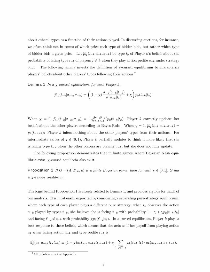
of bidder bids a given price. Let bptk(t−k|a−k,σ−k) be type tk of Player ks beliefs about theprobability of facing type t−k of players j 6= k when they play action proÞle a−k under strategyσ−k. The following lemma inverts the deÞnition of χ-cursed equilibrium to characterize

players beliefs about other players types following their actions.7

Lemma 1 In a χ-cursed equilibrium, for each Player k,

bptk(t−k|a−k,σ−k) = µ(1− χ) σ−k(a−k|t−k)σ(a−k|tk) + χ

¶pk(t−k|tk).

When χ = 0, bptk(t−k|a−k,σ−k) = σ−k(a−k|t−k)σ(a−k|tk)

pk(t−k|tk): Player k correctly updates herbeliefs about the other players according to Bayes Rule. When χ = 1, bptk(t−k|a−k,σ−k) =pk(t−k|tk): Player k infers nothing about the other players types from their actions. For

intermediate values of χ ∈ (0, 1), Player k partially updates to think it more likely that sheis facing type t−k when the other players are playing a−k, but she does not fully update.

The following proposition demonstrates that in Þnite games, where Bayesian Nash equi-

libria exist, χ-cursed equilibria also exist.

Proposition 1 If G = (A,T, p, u) is a Þnite Bayesian game, then for each χ ∈ [0, 1], G has

a χ-cursed equilibrium.

The logic behind Proposition 1 is closely related to Lemma 1, and provides a guide for much of

our analysis. It is most easily exposited by considering a separating pure-strategy equilibrium,

where each type of each player plays a different pure strategy; when tk observes the action

a−k played by types t−k, she believes she is facing t−k with probability 1 − χ + χpk(t−k|tk)and facing t0−k 6= t−k with probability χpk(t0−k|tk). In a cursed equilibrium, Player k plays abest response to these beliefs, which means that she acts as if her payoff from playing action

ak when facing action a−k and type proÞle t−k is

uχk (ak, a−k; tk, t−k) ≡ (1− χ)uk(ak, a−k; tk, t−k) + χX

t−k∈T−kpk(t−k|tk) · uk(ak, a−k; tk, t−k).

7All proofs are in the Appendix.

8

This is the χ-weighted average of her actual payoff as a function of actions and types and

her average payoff as a function of actions and her own type, averaged over the other types

of other players. We prove Proposition 1 by noting that since a χ-cursed equilibrium in

G = (A,T, p, u) is equivalent to a Bayesian Nash equilibrium in the χ-virtual game Gχ ≡

(A,T, p, uχ), G has a cursed equilibrium whenever Gχhas a Bayesian Nash equilibrium. We

use this reinterpretation and alternative formalization of cursed equilibrium as the Bayesian

Nash equilibrium of Gχrepeatedly below.

Proposition 1 follows from the fact that whenever G is Þnite, Gχis Þnite, and Þnite games

have at least one Bayesian Nash equilibrium. Proposition 1 is of limited general interest,

however. While every game we consider in this paper has an equilibrium for each value

of χ, most of the games we consider have uncountably inÞnite type and action spaces, so

Proposition 1 does not guarantee existence in these games. Moreover, the existence of a

Bayesian Nash equilibrium (χ = 0) is neither necessary nor sufficient for the existence of a

χ-cursed equilibrium for each χ ∈ (0, 1]. However, the counterexamples we have devised toshow this involve games with discontinuous payoffs or non-compact action spaces, and we

suspect that in well-behaved games where Bayesian Nash equilibria exist cursed equilibria

also exist.8

In a cursed equilibrium, a player maximizes her payoffs under the mistaken belief that

other players actions depend less on their types than they actually do. We establish in

Proposition 2 that if no player can learn anything about her expected payoff from any action

proÞle by learning any other players type, then the set of cursed equilibria coincides with the

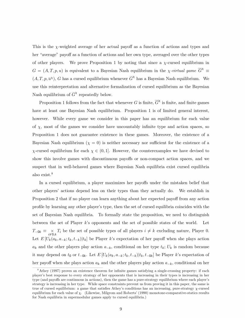
set of Bayesian Nash equilibria. To formally state the proposition, we need to distinguish

between the set of Player ks opponents and the set of possible states of the world. Let

T−0k ≡ ×i 6=0,k

Ti be the set of possible types of all players i 6= k excluding nature, Player 0.

Let E [Uk(ak, a−k; tk, t−k)|tk] be Player ks expectation of her payoff when she plays actionak and the other players play action a−k, conditional on her type tk; Uk is random because

it may depend on t0 or t−0k. Let E [Uk(ak, a−k; tk, t−k)|tk, t−0k] be Player ks expectation of

her payoff when she plays action ak and the other players play action a−k, conditional on her8Athey (1997) proves an existence theorem for inÞnite games satisfying a single-crossing property: if each

players best response to every strategy of her opponents that is increasing in their types is increasing in hertype (and payoffs are continuous in actions), then the game has a pure-strategy equilibrium where each playersstrategy is increasing in her type. While space constraints prevent us from proving it in this paper, the same istrue of cursed equilibrium: a game that satisÞes Atheys conditions has an increasing, pure-strategy χ-cursedequilibrium for each value of χ. (Likewise, Milgrom and Roberts (1990) monotone-comparative-statics resultsfor Nash equilibria in supermodular games apply to cursed equilibria.)

9

type tk and the other players (excluding natures) type t−0k.

Proposition 2 If for each Player k, each type tk ∈ Tk, each type proÞle t−0k ∈ T−0k, and

each action proÞle (ak, a−k) ∈ A, E [Uk(ak, a−k; tk, t−k)|tk, t−0k] = E [Uk(ak, a−k; tk, t−k)|tk] ,then for each χ ∈ [0, 1] the set of χ-cursed equilibria coincides with the set of Bayesian Nashequilibria.

The condition that E [Uk(ak, a−k; tk, t−k)|tk, t−0k] = E [Uk(ak, a−k; tk, t−k)|tk] not only re-quires that no players payoff be affected by any other players type, but also that no player

can learn anything about her expected payoff by learning any other players type; this means

essentially that (given a players type) other players types are uncorrelated with the state of

nature. This distinction is crucial in many of our applications. In a common-values auction,

for instance, bidders may not care about other bidders signals per se, but only about the

uncertain value of the object. But if one bidder learned another bidders signal her beliefs

about the value of the object, and therefore her beliefs about her payoffs from a proÞle of

bids, would change. Hence, Proposition 3 does not apply to common-values auctions. But it

does apply to private-values auctions, where each bidders payoff is a deterministic function

of her own type and the proÞle of bids.

The intuition behind the proposition is that if a player learns nothing about her expected

payoff from knowing the other players types, then it does not matter that she misunderstands

the relationship between the other players types and their actions. More precisely, a player

who correctly predicts the probability distribution over the other players actions who does

not learn anything about her expected payoff from learning the other players types chooses

the same action irrespective of her theory of which types of the other players play which

action.

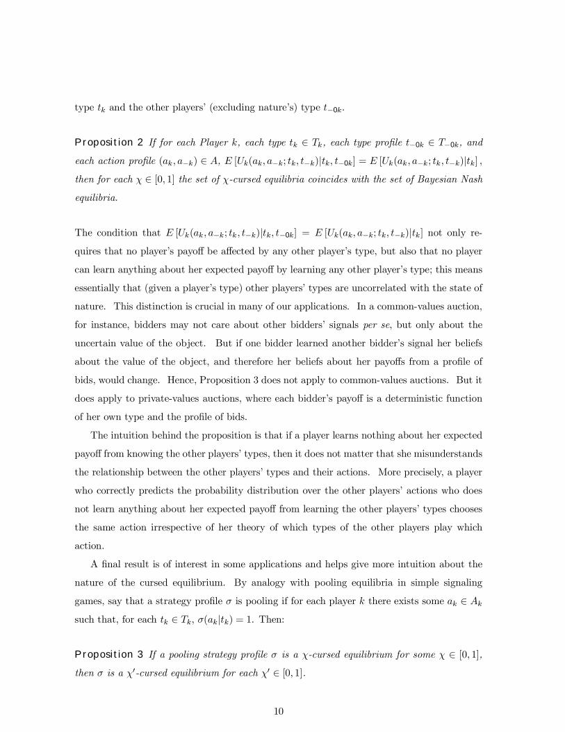
A Þnal result is of interest in some applications and helps give more intuition about the

nature of the cursed equilibrium. By analogy with pooling equilibria in simple signaling

games, say that a strategy proÞle σ is pooling if for each player k there exists some ak ∈ Aksuch that, for each tk ∈ Tk, σ(ak|tk) = 1. Then:

Proposition 3 If a pooling strategy proÞle σ is a χ-cursed equilibrium for some χ ∈ [0, 1],then σ is a χ0-cursed equilibrium for each χ0 ∈ [0, 1].

10

Proposition 3 implies that every pooling Bayesian Nash equilibrium meaning no

players action depends on her type is a χ-cursed equilibrium for every value of χ, and any

pooling χ-cursed equilibrium is a Bayesian Nash equilibrium. This is because in a pooling

equilibrium players actions are independent of their types. Ignoring the relationship between

others actions and their information is not a mistake when there is no relationship.

In many Bayesian games, especially sequential games, researchers apply reÞnements of

Bayesian Nash equilibrium in making predictions. A simple way to deÞne analogous reÞne-

ments of χ-cursed equilibrium is to deÞne the reÞnement in the χ-virtual game introduced

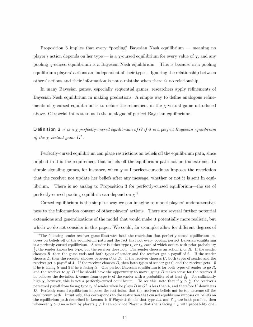
above. Of special interest to us is the analogue of perfect Bayesian equilibrium:

Definition 3 σ is a χ perfectly-cursed equilibrium of G if it is a perfect Bayesian equilibrium

of the χ-virtual game Gx.

Perfectly-cursed equilibrium can place restrictions on beliefs off the equilibrium path, since

implicit in it is the requirement that beliefs off the equilibrium path not be too extreme. In

simple signaling games, for instance, when χ = 1 perfect-cursedness imposes the restriction

that the receiver not update her beliefs after any message, whether or not it is sent in equi-

librium. There is no analog to Proposition 3 for perfectly-cursed equilibriumthe set of

perfectly-cursed pooling equilibria can depend on χ.9

Cursed equilibrium is the simplest way we can imagine to model players underattentive-

ness to the information content of other players actions. There are several further potential

extensions and generalizations of the model that would make it potentially more realistic, but

which we do not consider in this paper. We could, for example, allow for different degrees of

9The following sender-receiver game illustrates both the restriction that perfectly-cursed equilibrium im-poses on beliefs off of the equilibrium path and the fact that not every pooling perfect Bayesian equilibriumis a perfectly-cursed equilibrium. A sender is either type t1 or t2, each of which occurs with prior probability12; the sender knows her type, but the receiver does not. The sender chooses an action L or R. If the senderchooses R, then the game ends and both types of sender and the receiver get a payoff of 2. If the senderchooses L, then the receiver chooses between U or D. If the receiver chooses U , both types of sender and thereceiver get a payoff of 4. If the receiver chooses D, then both types of sender get 0, and the receiver gets −5if he is facing t1 and 5 if he is facing t2. One perfect Bayesian equilibrium is for both types of sender to go R,and the receiver to go D if he should have the opportunity to move: going D makes sense for the receiver ifhe believes the deviation L comes from type t2 of the sender with a probability of at least 9

10. For sufficiently

high χ, however, this is not a perfectly-cursed equilibrium. To see this, note that if χ > 15, the receivers

perceived payoff from facing type t2 of sender when he plays D in Gχis less than 4, and therefore U dominates

D. Perfectly cursed equilibrium imposes the restriction that the receivers beliefs not be too extreme off theequilibrium path. Intuitively, this corresponds to the restriction that cursed equilibrium imposes on beliefs onthe equilibrium path described in Lemma 1: if Player k thinks that type t−k and t0−k are both possible, thenwhenever χ > 0 no action by players j 6= k can convince Player k that she is facing t−k with probability one.

11

sophistication between players, or for different degrees of sophistication for different types of

a given player. While we discuss such reÞnements brießy in the conclusion, for the remainder

of the paper we consider some key applications of our simple variant of the model, relating

our results when possible to existing empirical evidence.

3 Trade

In many economic exchanges, one party has private information about the value of the good

she might sell or buy that determines the price at which she is willing to trade. In this section

we ßesh out the implications of cursed equilibrium in such settings, with both one-sided and

two-sided asymmetric information. We show that trade both may take place when Bayesian

Nash equilibrium predicts no trade and may not take place when Bayesian Nash equilibrium

predicts trade.

We begin by studying one-sided asymmetric information of the sort introduced in Ak-

erlofs (1970) lemons model, which we formalize along the lines of the model Samuelson and

Bazerman (1985) formulated in designing an experimental test. A Þrm offers itself for sale

to a raider; the Þrm knows its book value, but the raider does not. The raider has correct

priors that the book value of the Þrm is uniformly distributed on [0, 1]. Whatever its book

value, the Þrm values itself at its book value, while the raider values the Þrm at γ ≥ 1 timesbook value. The raider must make the Þrm an offer, which the Þrm then accepts or rejects;

without loss of generality we take the raiders offer space to be [0, 1]. The raider seeks to

maximize her expected surplus, and the Þrm accepts any offer above its book value.

Formally, there are two players F (Þrm) and R (raider), with TF ≡ [0, 1]. The raider, whohas no private information, chooses a price b ∈ [0, 1] at which she offers to buy the Þrm. TheÞrm chooses a response policy a : [0, 1] → 0, 1, where a(b) = 1 means that he accepts theraiders offer of b. The Þrms optimal strategy is clear: it sells at price b if and only if her

type is less than b. Given the uniform distribution of the Þrms type, therefore, the average

value of the Þrms sold at price b is b2 , which in turn means the raiders expected surplus from

offering b is b¡γ b2 − b

¢. By familiar lemons logic, the lower the bid the lower the average

value of the raider will get. When γ < 2, the expected net return to the raider will be negative

for any positive b, so the unique Bayesian Nash equilibrium outcome involves b = 0. When

γ > 2, the raiders expected proÞt is positive whatever her bid, and it is maximized at b = 1.

12

What are the χ-cursed equilibria? One is that the Þrm rejects all bids and the raider offers

zero; this, however, is not perfectly cursed since the best response of some types of Þrms to

a positive offer is to accept. Henceforth we limit our attention to perfectly-cursed equilibria.

Consider Þrst the extreme case where χ = 1, so the raider incorrectly thinks that the Þrms

decision whether to accept the offer does not depend on its book value. Let σF (a) be the

average (across types) probability that a Þrm plays action a.Thus, σF (1) =R b

0 1dt+R 1b 0dt = b,

because Þrms valued less than b sell while those valued above b do not. In a fully cursed

equilibrium, the raider thinks that if she offers b, each Þrm accepts with probability b. Her

perceived payoff from offering b is therefore b¡γ

2 − b¢, which is maximized by b = γ

4 for γ ≤ 4(and at b = 1 for γ > 4). The raiders true payoff from bidding γ

4 isγ4

¡γ γ8 − γ

4

¢= γ3−2γ2

32 < 0

for γ < 2. Thus the raider suffers a winners curse: she does not realize that the Þrm only

accepts her offer when its value is low. The fact that the raider thinks that some Þrms with

values above her bid will sell keeps her from lowering her bid to zero.10

For γ ∈ (2, 4), the raider bids too low: her payoff from bidding b = γ4 is

γ3−2γ2

32 , which

is less than γ−22 , her payoff from bidding b = 1. Cursedness leads to both overbidding when

γ < 2 and underbidding when γ > 2 for the same reason: a cursed buyer does fully appreciate

the extent to which raising her offer raises the expected value of the goods she buys, and so

she pays more attention to how her bid affects her probability of completing a trade than to

how it affects the quality of the good she will get.

Now consider χ ∈ (0, 1). If the raider offers b, a Þrm sells iff its valuation is less than b.

But in a χ-cursed equilibrium, the raider thinks a Þrm of type tF sells with probability

(1− χ)σF (1|tF ) + χσF (1) =½1− χ+ χb for tF < bχb for tF > b.

The raider thinks that with probability χ, the Þrm accepts a bid b with probability b inde-

pendent of its type, and with probability 1−χ, a Þrm accepts b iff tF < b. Hence, the raidersperceived expected surplus from bidding b is

b (1− χ+ χb)µγb

2− b¶+ (1− b)χb

µγb+ 1

2− b¶,

which is maximized by b∗ = χγ4−2γ(1−χ) . From this, it can be seen that ∂b

∗∂χ > 0 if and only if

γ > 2, which means that the buyer overpays when γ < 2 and underpays when γ > 2.10Note that even when γ < 1, the cursed equilbrium involves b > 0; even though the raider knows that

the Þrm is always worth less to her than to the Þrm, she still makes a positive offer. Hence, despite itbeing common knowledge that there are no gains from trade, players trade nonetheless. While we know ofno evidence on this prediction and this degree of error does not seem entirely implausible to us, it does seemsomewhat unlikely.

13

Existing experimental evidence on this model shows that subjects do bid positive amounts,

contradicting the Bayesian-Nash prediction of 0. But in fact they tend to bid in excess of

the levels predicted by even the fully-cursed equilibrium. When γ = 32 , the fully cursed-

equilibrium is b∗ = 38 . Samuelson and Bazerman (1985) Þnd that the majority of subjects

make offers in (0.5, 0.75). Ball, Bazerman, and Carroll (1991) allow subjects to learn by

repeating the game twenty times, where subjects learn their payoffs after every round. Such

learning does not appreciably affect average bids, which over the course of the trials fall

modestly from 0.57 to 0.55.

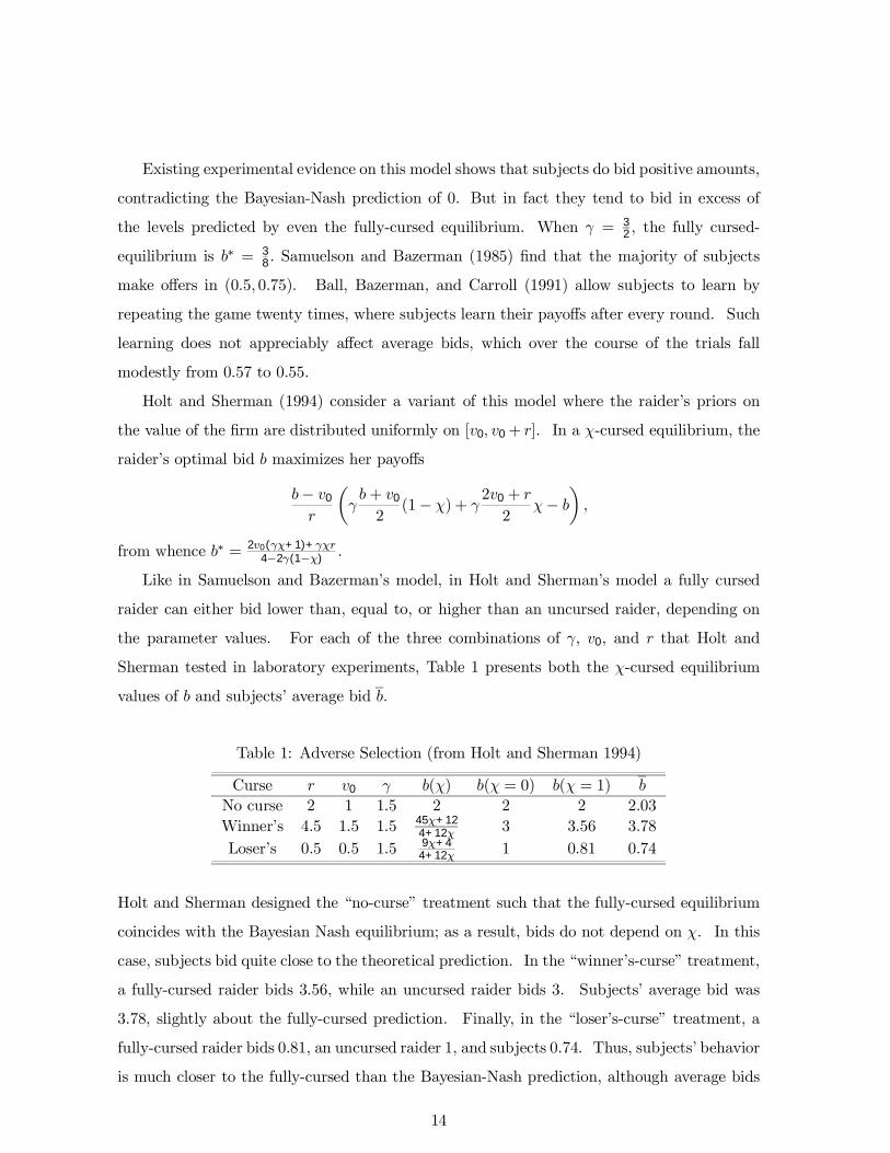
Holt and Sherman (1994) consider a variant of this model where the raiders priors on

the value of the Þrm are distributed uniformly on [v0, v0+ r]. In a χ-cursed equilibrium, the

raiders optimal bid b maximizes her payoffs

b− v0

r

µγb+ v0

2(1− χ) + γ 2v0 + r

2χ− b

¶,

from whence b∗ = 2v0(γχ+1)+γχr4−2γ(1−χ)

.

Like in Samuelson and Bazermans model, in Holt and Shermans model a fully cursed

raider can either bid lower than, equal to, or higher than an uncursed raider, depending on

the parameter values. For each of the three combinations of γ, v0, and r that Holt and

Sherman tested in laboratory experiments, Table 1 presents both the χ-cursed equilibrium

values of b and subjects average bid b.

Table 1: Adverse Selection (from Holt and Sherman 1994)

Curse r v0 γ b(χ) b(χ = 0) b(χ = 1) b

No curse 2 1 1.5 2 2 2 2.03

Winners 4.5 1.5 1.5 45χ+124+12χ 3 3.56 3.78

Losers 0.5 0.5 1.5 9χ+44+12χ 1 0.81 0.74

Holt and Sherman designed the no-curse treatment such that the fully-cursed equilibrium

coincides with the Bayesian Nash equilibrium; as a result, bids do not depend on χ. In this

case, subjects bid quite close to the theoretical prediction. In the winners-curse treatment,

a fully-cursed raider bids 3.56, while an uncursed raider bids 3. Subjects average bid was

3.78, slightly about the fully-cursed prediction. Finally, in the losers-curse treatment, a

fully-cursed raider bids 0.81, an uncursed raider 1, and subjects 0.74. Thus, subjects behavior

is much closer to the fully-cursed than the Bayesian-Nash prediction, although average bids

14

depart too extremely from Bayesian Nash equilibrium to be adequately described by cursed

equilibrium.

We now turn to two-sided asymmetric information and show that trade can occur in a χ-

cursed equilibrium, even when it is common knowledge that the value of the good is identical

for the two partiesso that Bayesian Nash equilibrium predicts no trade. While we know of

no experimental evidence in such a situation, our prediction of trade matches the common

intuition that speculative trade occurs when the no-trade theorems of Milgrom and Stokey

(1982) and others predict none. Let Ω = ω1,ω2,ω3 be the set of possible payoff-relevantstates of the world, where the two players share the common prior µ(ω1) = µ(ω2) = µ(ω3) =

13 .

Suppose that Player 2 holds an asset which pays k in state ωk, so that the higher the state

the higher the value of the asset. Each player has private information about the state of

the world: Player 1 learns when the state is ω1, but cannot differentiate between states ω2

and ω3; Player 2 learns when the state is ω3, but cannot differentiate between states ω1 and

ω2. The information partitions P1 = ω1, ω2,ω3 and P2 = ω1,ω2, ω3 representPlayer 1 and Player 2s information, respectively; Pi is an element of Player is partition Pi.After each player receives her private information, Player 1 makes Player 2 an offer for the

asset which Player 2 then accepts or rejects.

The only possible trade that can occur in a Bayesian Nash equilibrium of this game is the

relatively meaningless one where the good is traded at price 2 in state ω2 and neither party

expects to beneÞt from the trade. For any χ ∈ (0, 1], however, trade in which a party expectsto gain can occur in state ω2. Let b1 : P1 → [1, 3] denote Player 1s bidding strategy, and

a2 : P2 × [1, 3] → 0, 1 denote Player 2s acceptance strategy, where a2 = 1 means Player

2 accepts Player 1s bid. Each players payoff in state ωk is k if she holds the asset after

trading plus or minus any transfer she paid received or paid.

The following strategies are a cursed equilibrium with trade in state ω2:

b1(P1) =

½1 P1 = ω12− χ

2 P1 = ω2,ω3,and

a2 (P2, b1) =

½1 P2 = ω1,ω2, b1 ≥ 2− χ

20 P2 = ω3 or b1 < 2− χ

2 .

First note that trade cannot occur in states ω1 or ω3. The most that Player 1 is willing

to offer in ω1 is 1, but because Player 2 puts positive probability on being in state ω2 when

the state is ω2 whatever b1 (ω2,ω3), Player 2 rejects Player 1s offer. In ω3, Player 2 will

15

accept no less than 3, but Player 1 will not offer 3 since Player 2 would accept that in state

ω2. Now consider ω2. As long as b1(ω1) 6= b1(ω2,ω3), Player 2 thinks the probabilityof being in state ω2 given he receives the bid b1(ω2,ω3) is 1− χ

2 . Thus his expected value

of the asset is¡1− χ

2

¢2 + χ

2 = 2 − χ2 . If Player 2 accepts Player 1s offer in state ω2, then

given that he rejects it in ω3, Player 1 thinks that when her offer is accepted the probability

of being in ω2 is 1− χ2 , and thus the expected value of the asset is

¡1− χ

2

¢2 + χ

2 · 3 = 2 + χ2 .

Hence Player 1 strictly prefers to trade, and she offers 2− χ2 , the lowest price at which Player

2 is willing to trade.

In this example, trade in ω2 occurs in a cursed equilibrium because neither player suffi-

ciently updates her beliefs about the value of the object given the willingness of the other

player to trade. In the information structure given, Player 1 is overly optimistic about the

value of the object based on her private information alone when it turns out that the state

is ω2. But whereas an uncursed trader would learn from Player 2s willingness to trade at a

low price that the state is ω2, a cursed trader remains overoptimistic that the state is ω3.11

While trade only occurs one third of the time in the example, it is easy to see that whatever

the probability of ω2, so long as both ω1 and ω3 both occur with positive probability, trade

can occur. Since cursed equilibrium is consistent with speculative trade where at least

one player strictly prefers trading to not trading with probability arbitrarily close to one,

a natural question is whether it is consistent with speculative trade with probability one. It

is not. To see why, consider again the trading mechanism described in our example where

Player 1 makes Player 2 an offer, and suppose that both players are fully cursed. If Player

2 always accepts Player 1s offer, then Player 1 learns nothing about the value of the object

from the fact that they are trading, and therefore she can offer no more than her expectation

of the assets value at any of her information sets. If she strictly prefers trading at some

information set, then she must offer less than her expectation of the value of the object at

that information set, and therefore her average offer (across all information sets) must be less

than the assets expected value. Likewise, since Player 2 is fully cursed, he infers nothing

from Player 1s offer, and hence at each of his information sets he must be offered more than11While in this trading mechanism Player 1 beneÞts from trade, there exist other trading mechanisms under

which Player 2 gains. It is also not important to the example that both players are cursed: trade will occur instate ω2 if only one of the two players is cursed. This follows from the fact that when Player 1 makes Player2 an offer, Player 2 thinks that the probability of being in state ω2 is less than one, so he will accept someoffer sufficiently close to, but below, 2 when he is cursed. If Player 1 is cursed, she thinks that the probabilityof being in ω2 given that her offer is accepted is less than one, and hence she is willing to offer more than 2,which Player 1 will accept.

16

his expectation of the assets value. If he strictly prefers trading at some information set,

then he must be offered more than his expectation of the assets value, and thus Player 1s

average offer must exceed the expected value of the asset, a contradiction. When players a

cursed, but not fully cursed, essentially the same argument applies.

4 Common-Values Auctions

In this section, we use an example to illustrate the implications of cursed equilibrium in Þrst-

and second-price auctions. Under either auction format in our example, the more cursed

are bidders, the higher they bid, and when the number of bidders is sufficiently high cursed

bidders suffer the winners curse the average winning bid exceeds the average value of the

object. We show that second-price auctions raise more expected revenue than Þrst-price

auctions with cursed bidders, just as with rational bidders. However, unlike with rational

bidders, as cursed bidders information about the value of the object becomes more precise,

the sellers expected revenue may fall, so a seller may have incentive to hide information about

the value of the object from cursed bidders. Finally, we provide an example of a common-

values auction where cursed bidders bid less than uncursed bidders. In the Þnal part of this

section, we discuss some of the experimental literature on common-values auctions in relation

to cursed equilibrium.

In a common-values auction, the value of the object being auctioned is common but un-

known to all bidders. In our example, we assume bidders receive signals that are independent

and identically distributed conditional on the common value of the object. Bidders are risk

neutral, and a bidders utility from winning the auction is simply the value of the object,

s, minus the price she pays, p; her utility from losing the auction is zero. Throughout this

section, we use capital letters to denote random variables and lower-case letters to denote

values these random variables take on. In order to analyze cursed equilibrium in common-

values auctions, we use the χ-virtual game introduced in Section 2 where Bidder is utility

from winning the auction at price p when the value of the object is s is

(1− χ)s+ χE[S|Xi = xi]− p,

where xi is the value of Bidder is signal about the value of the object. That is, Bidder

is valuation of the object is the χ-weighted average of the objects actual value and her

17

expectation of its value conditional on her signal.

Suppose that n bidders share a common prior on the value of the object. We follow

Klemperers (1999) example and assume that value of the object, S, is distributed uniformly

on the real line, and Bidder is signal, Xi, is distributed uniformly on£S − a

2 , S +a2

¤for

some a > 0.12 Three functions that play an important role in our analysis merit deÞnition

here: Y ni (1) is the highest signal among bidders j 6= i; r(xi) ≡ E[S|Xi = x] is Bidder is

expectation of the value of the object conditional on her signal Xi = x; and vn(x, y) ≡E[S|Xi = x, Y ni (1) = y] is Bidder is expectation of the value of the object conditional on hersignal being x and the highest of the other bidders signals being y.

We say that a bidder suffers the winners curse in a given equilibrium of a given auction if

the bidders expected surplus from entering the auction is negative; that is, the expectation of

the value of the object less the price, both conditional on the event that she wins, is negative.

In order that our deÞnition apply across auction settings, we parameterize auctions by P n,

the price the winner pays when she wins the n-bidder auction; for example, in a Þrst-price

auction, Pn is the winners bid.

Definition 4 Bidder i suffers the winners curse in equilibrium (bi, b−i) of the n-bidder auc-

tion if E[(S − P n) 1bi(Xi)>maxj 6=i bj (Xj )] < 0.13

Under our deÞnition, a bidder suffers the winners curse if the expected value of the

object conditional on winning is less than the price conditional on winning. In a symmetric

equilibrium of a symmetric model, Bidder i suffers the winners curse if E[S] < E[Pn], namely

if the expected price exceeds the expected value of the object.14

We begin our analysis with second-price auctions, where the highest bidder wins the

auction and pays the second-highest bid. Milgrom and Weber (1982) show that a Bayesian

Nash equilibrium of the second-price auction in this setting is bi(xi) = vn(xi, xi) Bidder i

bids her expectation of the value of the object conditional on both her signal and the highest

12While the uniform distribution over the real line is not deÞned, it can be thought of as the limit of theuniform distribution on [−K,K] as K →∞. When the value of the object is negative, the auction correspondsto a procurement auction where the seller pays the winner to perform some costly activity. For the purposesof the example, however, all that matters is that the bidders beliefs about S as a function of their signals areuniform. For a more thorough analysis of Bayesian Nash equilibrium in this model, see Klemperer (1999).131A is the indicator function that takes on the value one when A occurs and zero otherwise.14Our deÞnition of the winners curse is not the only reasonable one. A more liberal deÞnition would be

that a bidder suffers the winners curse if her expected surplus from entering the auction is less than Nash-equilibrium analysis suggests. We use our deÞnition because it emphasizes the severity of overbidding andmatches the folk wisdom that winning bids in common-values auctions tend to exceed the value of the object.

18

of the other bidders signals being xi. To see that this is an equilibrium, suppose that bidders

j 6= i follow their proposed equilibrium strategies. A Bidder i with signal xi who bids bi

receives a payoff of Z b−1j (b1)

xi−a(vn(xi, y)− vn(y, y)) fY ni (1)(y|Xi = xi)dy,

where fY ni (1)(y|Xi = xi) is the density of Y ni (1) conditional onXi = xi. It is easy to show thatvn(xi, y) is increasing in xi, which implies that the integrand is positive if and only if xi > y.

Hence, Bidder is expected utility is maximized when b−1j (bi) = xi, or bi = bj(xi). Intuitively,

Bidder is bid does not affect the price she pays when she wins, only which auctions she wins.

If the other bidders follow their equilibrium strategies, then the only effect of raising her

bid above vn(xi, xi) is for Bidder i to win some auctions where yni (1) > xi; but in that case

vn(xi, yni (1)) < vn(yni (1), y

ni (1)). In words, by raising her bid above v

n(xi, xi), Bidder i can

only win auctions she would prefer to lose. Likewise, by lowering her bid, Bidder i can only

lose auctions she would prefer to win.

In the χ-virtual game corresponding to the second-price auction, Bidder is expectation of

the value of the object conditional on her signal being xi and the highest of the other bidders

signals being y is

E (1− χ)S + χE[S|Xi = xi]|Xi = xi, Y ni (1) = y = (1− χ)vn(xi, y) + χr(xi).

Because r(xi) and vn(xi, y) are both increasing in xi, the expression is increasing in xi,

and therefore we can use the same argument as Milgrom and Weber to show that bi(xi) =

(1−χ)vn(xi, xi) +χr(xi) is a χ-cursed equilibrium of the second-price auction. Here, rather

than bid her expectation of the value of the object conditional on her signal being both the

highest and second-highest, Bidder i bids the χ-weighted average of that and her expectation

of the value of the object conditional on her signal alone. Intuitively, the second part of

Bidder is bidding function reßects the fact that she thinks that there may be no information

content in winning.

In our example, after observing signal xi Bidder i forms posteriors that S is distributed

uniformly on£xi − a

2 , xi +a2

¤, and so her expected value of the object conditional on her

signal, r(xi), is xi. Bidder is posteriors on S given that Xi = Y ni (1) = xi are given by

hn(s|Xi = xi, Y ni (1) = xi) =¡xi−sa + 1

2

¢n−2R xi+a2

xi−a2

¡xi−sa + 1

2

¢n−2ds=n− 1a

µxi − sa

+1

2

¶n−2

,

19

for s ∈ £xi − a2 , xi +

a2

¤(and hn(s|Xi = xi, Y ni (1) = xi) = 0 for s /∈

£xi − a

2 , xi +a2

¤). Bidder

is expectation of the value of the object conditional on her signal being both the highest and

second highest on the n bidders signals is vn(xi, xi) = xi − a2 +

an . Thus, the symmetric

χ-cursed equilibrium in the second-price auction is

bn(xi) = xi − (1− χ)an− 22n

.

When n = 2, Bayesian Nash and cursed equilibrium coincide.15 For n ≥ 3, bids are increasingin χ for every signal value, so the sellers revenue is also increasing in χ. For χ < 1, bids

are decreasing in n, but the higher χ, the slower bids decrease as n increases. For a given s,

the expected second-highest signal E[Y n(2)|S = s] = s− a2 +

n−1n+1a, and the sellers expected

revenue in the n-bidder auction is

E[bn(Y n(2))|S = s] = s− a n− 1n(n+ 1)

+ χan− 22n

.

The sellers expected revenue is increasing in n for all χ, and as n → ∞ it approaches

s + χa2 > s, which implies that bidders suffer the winners curse. In general, for n > n =

χ+2+√

9χ2−4χ+42χ , the sellers expected revenue exceeds s and bidders suffer the winners curse.

When χ = 1, for example, n = 3, meaning that bidders suffer the winners curse whenever

n ≥ 4. As χ→ 0, the χ-cursed equilibrium approaches the Bayesian Nash equilibrium where,

of course, bidders never suffer the winners curse; in this case, n→∞.An implication of the winners curse is that by committing to a policy of revealing in-

formation about the value of the object, the seller may lower her expected revenue. This

contrasts Bayesian-Nash analysis, where improving rational bidders information about the

value of the object mitigates bidders fear of the winners curse and hence intensiÞes the

competitiveness of their bidding, raising the sellers expected revenue. In our model, as a

increases, each bidders private information about the value of the object becomes noisier, so

that increasing a can be thought of as making bidders less informed. When χ = 0, increasing

a causes bidders to lower their bids enough that the sellers expected revenue falls. When

χ > χ ≡ 2(n−1)(n−2)(n+1)

, however, increasing a lowers bids but increases the sellers revenue. For

example, when n = 4, the sellers revenue is increasing in a whenever χ > 35 . As n → ∞,

15When n = 2, r(xi) = vn(xi, xi), since a bidder learns nothing about the value of the object by learningthat the other bidders signal is lower than her own; intuitively, for each value of s ∈ £xi − a

2, xi + a

2

¤is the

probability that Xj < xi equal to one half. This result depends on the particular functional forms of ourexample, and in general Bayesian Nash and cursed equilibria can differ in two-bidder common-value auctions.

20

χ → 0, so increasing a always leads to an increase in the sellers revenue, no matter slight

bidders cursedness. The winners curse is one implication of this result. When a = 0,

bidders know the value of the object with certainty, so the sellers expected revenue is the

value of the object. For large n, increasing a increases the sellers revenue, so bidders suffer

the winners curse for a > 0.16

One natural question is whether the sellers expected revenue is always increasing in

χ. Since bi(xi) = (1 − χ)vn(xi, xi) + χr(xi) is the χ-cursed equilibrium of the general

second-price auction, the sellers expected revenue is increasing in χ whenever E[r(Y n(2)] >

E[vn(Y n(2), Y n(2)], namely when the expectation of the second-highest signal holders ex-

pectation of the value of the object conditional on her signal alone is higher than the ex-

pectation of the second-highest signal holders expectation of the value of the object con-

ditional on her signal being the highest and second-highest. In our example, r(xi) = xi

and vn(xi, xi) = xi − a2 +

an < xi, so the sellers expected revenue does not depend on χ for

n = 2 and is increasing in χ for n > 2. But consider another example where s, xi ∈ 0, 1,Pr[S = 0] = Pr[S = 1] = 1

2 , and Pr[Xi = 0|S = 0] = 12 and Pr[Xi = 0|S = 1] = 0. When the

value of the object is low, both signals are equally likely, but when the value of the object is

high, the high signal occurs with probability one. In a Bayesian Nash equilibrium, a bidder

with xi = 0 knows the object is worth zero, and thus b(0) = 0. A bidder with signal xi = 1

16As an alternative illustration that the seller may prefer withholding information from the bidders, supposethat, like the bidders, the seller receives a signal about the value of the object Z ∼ U £s− a

2, s+ a

2

¤. Before

receiving her signal, the seller chooses between truthfully revealing and concealing her signal, whatever itis. Milgrom and Weber (1982) show that when bidders are rational the seller prefers truthful revelation.When bidders are cursed, the χ-cursed equilibrium in the auction when the seller reveals is ebn(xi, z) = (1 −χ)evn(xi, xi, z) + er(xi, z). The function evn(xi, xi, z) is the analogue to vn(xi, xi) when the sellers signal isz, and er(xi, z) is the analogue to r(xi) when the sellers signal is z. It is easy to show that for all xi andz, evn(xi, xi, z) = vn(xi, xi): intuitively, if a bidder has beliefs µ(s) over s ∈

£xi − a

2 , xi +a2

¤when her signal

and the highest of other signals is xi, then because every value of s is equally likely to generate the signalz, learning z does cause the bidder to update her beliefs. But whereas r(xi) = xi, er(xi, z) = 1

2(xi + z): a

bidders expectation of the value of the object conditional on the two signals (xi, z) is simply their average.Thus, the sellers expected revenue in state s when she can commit to truthfully revealing her signal is

E[ebn(Y n(2))|S = s] = s− a n− 1n(n+ 1)

+ χan2 + n− 44n(n+ 1)

.

By concealing her signal, the seller achieves the same expected revenue as when she has no signal. Whenn = 2, the sellers expected revenue is larger than when she has no signal because E [er(Y n(2), Z)|S = s] >E [r(Y n(2))|S = s] , since Y n(2) is on average less than Z. When n = 3, the sellers expected revenue does notdepend on whether she reveals her signal because E [er(Y n(2), Z)|S = s] = E [r(Y n(2))|S = s] , since Y n(2) ison average equal to Z. However, for n ≥ 4, the sellers expected revenue is lower than when she has no signalbecause E [er(Y n(2), Z)|S = s] < E [r(Y n(2))|S = s] , since Y n(2) is on average greater than Z. Thus, withenough bidders the seller decreases her expected revenue by committing to a policy of truthfully revealing hersignal.

21

knows that if xj = 0, the object is worth zero and her payoff is zero whatever she bids. If

xi = xj = 1, then the expected value of the object is 45 , and thus b(1) =

45 . When χ = 1,

we b(0) = 0 and b(1) = 23 is a cursed equilibrium. A bidder with xi = 0 knows the object

is worth zero, and thus b(0) = 0. A bidder with xi = 1 knows that the only time her bid

matters is when bj = 23 ; since she thinks that bj conveys no information about Bidder js

signal, a bidder with xi = 1 thinks the value of the object is 23 . Bidder is perceived expected

payoff to any bid is zero, so b(0) = 0 and b(1) = 23 is a fully-cursed equilibrium. Cursed and

rational bidders with xi = 0 both bid 0, but cursed bidders with xi = 1 bid 23 , while rational

bidders bid 45 . Hence, in this example, the sellers expected revenue is higher when bidders

are rational than when they are cursed.17

We now turn to Þrst price auctions, where the high bidder wins the auction and pays her

bid. In a symmetric χ-cursed equilibrium of the Þrst-price auction, a Bidder i with signal

Xi = xi chooses bi to maximizeZ b−1j (bi)

x

((1− χ)vn(xi, y) + χr(xi)− bi) fY ni (1)(y|Xi = xi),

where bj is the common equilibrium bidding function of bidders j 6= i and fY ni (1)(y|Xi = xi)is the density of Y ni (1) conditional on Xi = xi. A necessary condition for equilibrium is that

dbn(xi)

dxi= ((1− χ)vn(xi, xi) + χr(xi)− bn(xi))

fY ni (1)(xi|Xi = xi)FY ni (1)(xi|Xi = xi)

,

which in our example is

dbn(xi)

dxi=

µxi − (1− χ)an− 2

n− b(xi)

¶ R xi+ a2

xi− a2(n− 1) ¡xi−sa + 1

2

¢n−2 1a2dsR xi+ a

2xi−a

2

¡xi−sa + 1

2

¢n−1 1ads

,

which simpliÞes todbn(xi)

dxi=

µxi − (1− χ)an− 2

n− b(xi)

¶n

a.

Hence, the symmetric χ-cursed equilibrium of the Þrst-price auction is

bn(xi) = xi − a2+ χa

n− 22n

.

When χ = 0, bn(xi) = x− a2 , and bids are independent of the number of bidders. When

χ > 0, bids increase in n. Intuitively, when χ = 1, a bidder with signal xi values the object17We believe that in general revenue increases with χ. We are familiar with no experimental tests on

auctions where revenues decrease with χ, which might be an additional useful test of our explanation of thewinners curse in auctions.

22

at r(xi) = xi, so the auction is one of private, but correlated, values. As n increases, bidders

bid more because they face increased competition. For a given s, the expected highest signal

E[Y n(1)|S = s] = s+ n−1n+1

a2 , and the sellers expected revenue in the n-bidder auction is

E[bn(Y n(1))|S = s] = s− a

n+ 1+ aχ

n− 22n

.

Like in the second-price auction, the sellers expected revenue is increasing in n. Bidders

suffer the winners curse when n ≥ n ≡ 2+χ+√

9χ2+4χ+42χ . When χ = 1, n ≈ 3.5, so bidders

suffer the winners curse whenever n ≥ 4. In a second-price auction when χ = 1 bidders alsosuffer the winners curse whenever n ≥ 4. When χ = 1

2 , bidders suffer the winners curse

in a Þrst-price auction when n ≥ 6, while they suffer the winners curse in a second-price

auction when n ≥ 5. This difference reßects the fact that in a cursed equilibrium, as in a

Bayesian Nash equilibrium, the second-price auction raises more expected revenue than the

Þrst-price auction. In a cursed equilibrium, bids are decreasing in a, just as in the rational

case. When χ > χ ≡ 2n(n−2)(n+1) , again the sellers expected revenue is increasing in a. Just

as in second-price auctions, in a Þrst-price auction with a large number of bidders χ is close

to zero, so the sellers expected revenue in large auctions is increasing in a, as long as bidders

are not completely rational.

Rather than analyze more general implications of cursed equilibrium in auctions, we con-

clude this section by relating our analysis above to some of the large body of experimental

evidence. In an early experiment, Bazerman and Samuelson (1983) auctioned off jars of

coins to student subjects. In each auction, subjects could see the jar being auctioned, but

did not know how many coins it contained. The highest bidder paid her bid and received the

paper-dollar equivalent of the coins in the jar. Subjects also guessed how many coins each

jar contained, and the subject whose guess was closest to the true value won a cash prize.

Whereas all of the jars actually contained $8.00, the average winning bid was $10.01. How-

ever, the subjects average estimate of the money in the jar was only $5.13. Even though the

subjects were on average too pessimistic about the value of the money in the jars, they suf-

fered the winners curse, presumably because those with high bids bid close to their estimates,

rather than tempering their bids.

Kagel and Levin (1986) test a model nearly identical to our example above: the value

of the object is distributed uniformly over [s, s], and each bidder i receives a signal Xi ∼U£s− a

2 , s+a2

¤, when s is the value of the good. In a Þrst-price auction, the χ-cursed

23

equilibrium of this auction is

b(xi) = xi − a2+ χa

n− 22n

+a¡1− n−1

n χ¢

n+ 1zi,

for xi ∈£s+ a

2 , s− a2

¤and zi = exp

µ−n(xi−(s+ a

2 ))a

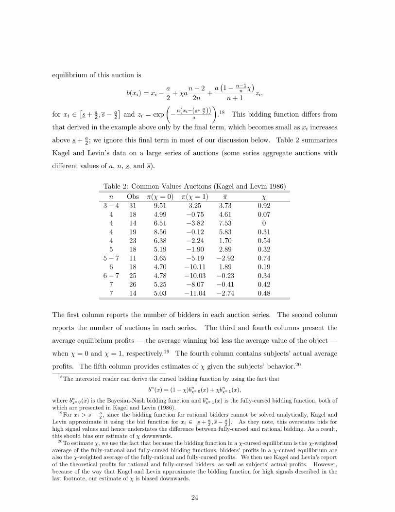
¶.18 This bidding function differs from

that derived in the example above only by the Þnal term, which becomes small as xi increases

above s+ a2 ; we ignore this Þnal term in most of our discussion below. Table 2 summarizes

Kagel and Levins data on a large series of auctions (some series aggregate auctions with

different values of a, n, s, and s).

Table 2: Common-Values Auctions (Kagel and Levin 1986)

n Obs π(χ = 0) π(χ = 1) π χ

3− 4 31 9.51 3.25 3.73 0.924 18 4.99 −0.75 4.61 0.074 14 6.51 −3.82 7.53 04 19 8.56 −0.12 5.83 0.314 23 6.38 −2.24 1.70 0.545 18 5.19 −1.90 2.89 0.32

5− 7 11 3.65 −5.19 −2.92 0.746 18 4.70 −10.11 1.89 0.19

6− 7 25 4.78 −10.03 −0.23 0.347 26 5.25 −8.07 −0.41 0.427 14 5.03 −11.04 −2.74 0.48

The Þrst column reports the number of bidders in each auction series. The second column

reports the number of auctions in each series. The third and fourth columns present the

average equilibrium proÞts the average winning bid less the average value of the object

when χ = 0 and χ = 1, respectively.19 The fourth column contains subjects actual average

proÞts. The Þfth column provides estimates of χ given the subjects behavior.20

18The interested reader can derive the cursed bidding function by using the fact that

bn(x) = (1− χ)bnχ=0(x) + χbnχ=1(x),

where bnχ=0(x) is the Bayesian-Nash bidding function and bnχ=1(x) is the fully-cursed bidding function, both of

which are presented in Kagel and Levin (1986).19For xi > s − a

2, since the bidding function for rational bidders cannot be solved analytically, Kagel and

Levin approximate it using the bid function for xi ∈£s+ a

2, s− a

2

¤. As they note, this overstates bids for

high signal values and hence understates the difference between fully-cursed and rational bidding. As a result,this should bias our estimate of χ downwards.20To estimate χ, we use the fact that because the bidding function in a χ-cursed equilibrium is the χ-weighted

average of the fully-rational and fully-cursed bidding functions, bidders proÞts in a χ-cursed equilibrium arealso the χ-weighted average of the fully-rational and fully-cursed proÞts. We then use Kagel and Levins reportof the theoretical proÞts for rational and fully-cursed bidders, as well as subjects actual proÞts. However,because of the way that Kagel and Levin approximate the bidding function for high signals described in thelast footnote, our estimate of χ is biased downwards.

24

Kagel and Levins data are broadly consistent with positive χ, but not χ = 1. In

every auction series but one, subjects proÞts lie between the Bayesian-Nash and fully-cursed

predictions. Our estimates of χ are fairly consistent across auction series, with 7 of the 11

between 0.19 and 0.54. The average value of χ (weighted by the number of observations for

each values) is 0.42.21 In this experiment, as in many others, when the number of bidders is

small, average proÞts are positive, but when the number of bidders is large, average proÞts

are negative. Kagel and Levin (1986) conclude that the larger the number of bidders, the

further the subjects bids from Nash equilibrium. However, if we estimate χ separately for

n ≤ 4 and n ≥ 5, we get estimates are 0.39 and 0.46, respectively. Thus, while χ appears tobe marginally higher for large n, the fact that the two estimates are so similar suggests that

subjects cursedness is not particularly sensitive to n. As we showed in our example above,

whatever χ, bidders suffer the winners curse for large enough n.

All said, cursed equilibrium seems to Þt reasonably well how proÞts depend on the number

of bidders and the noisiness of bidders signals, a.A further indication that the subjects exhibit

cursed behavior, which (unlike Table 2) includes bids from losing bidders, comes from Kagel

and Levins (1986) estimate of the linear bidding function

b(xi, a, n) = 1.00xi − 0.74a2+ 0.65n,

(0.002) (0.03) (0.15)

where standard errors are reported below the regression coefficients.22 Because the bidding

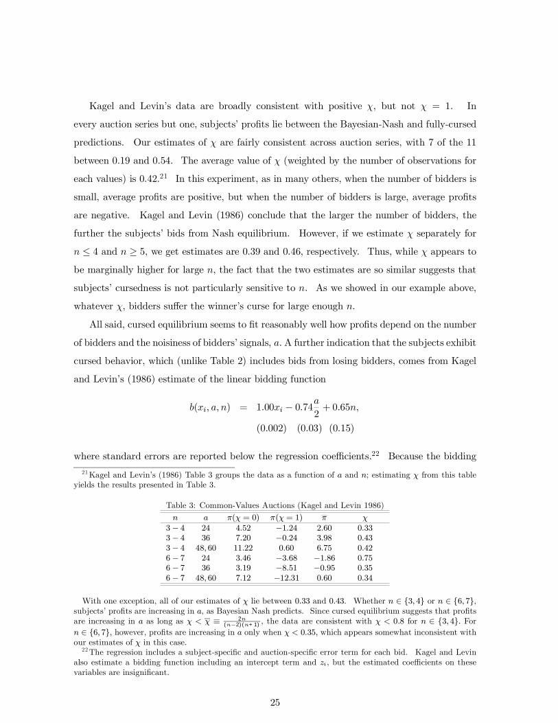
21Kagel and Levins (1986) Table 3 groups the data as a function of a and n; estimating χ from this tableyields the results presented in Table 3.

Table 3: Common-Values Auctions (Kagel and Levin 1986)

n a π(χ = 0) π(χ = 1) π χ

3− 4 24 4.52 −1.24 2.60 0.333− 4 36 7.20 −0.24 3.98 0.433− 4 48, 60 11.22 0.60 6.75 0.426− 7 24 3.46 −3.68 −1.86 0.756− 7 36 3.19 −8.51 −0.95 0.356− 7 48, 60 7.12 −12.31 0.60 0.34

With one exception, all of our estimates of χ lie between 0.33 and 0.43. Whether n ∈ 3, 4 or n ∈ 6, 7,subjects proÞts are increasing in a, as Bayesian Nash predicts. Since cursed equilibrium suggests that proÞtsare increasing in a as long as χ < χ ≡ 2n

(n−2)(n+1) , the data are consistent with χ < 0.8 for n ∈ 3, 4. Forn ∈ 6, 7, however, proÞts are increasing in a only when χ < 0.35, which appears somewhat inconsistent withour estimates of χ in this case.22The regression includes a subject-speciÞc and auction-speciÞc error term for each bid. Kagel and Levin

also estimate a bidding function including an intercept term and zi, but the estimated coefficients on thesevariables are insigniÞcant.

25

function in a cursed equilibrium is linear in neither a2 nor in n, Kagel and Levins estimated

bidding function is somewhat hard to interpret. But the coefficient on a2 is signiÞcantly

less than the value of one predicted by Bayesian Nash equilibrium, and bids are increasing

in n, rather than decreasing as predicted by Bayesian Nash equilibrium. Both results are

consistent with cursed equilibrium. Finally, we should note that in only 71% of auctions did

the high-signal holder win. In a cursed equilibrium, as in a Bayesian Nash, all of the auctions

should have been won by the high-signal holder, and that they were not suggests that subjects

made errors in addition to those predicted by cursed equilibrium, or that different bidders

were cursed to different degrees.

Many other papers Þnd evidence of the winners curse. Lind and Plott (1991) show

that the winners curse in Kagel and Levins (1986) experiments is not due to any strategic

effects of limited liability the fact that subjects who lost more than some initial endowment

were removed from the experiment. Dyer, Kagel and Levin (1989) report experiments using

students and executives from the construction industry; all but one of the executives had

experience bidding in auctions. They Þnd that both types of subjects suffer the winners

curse, and that the curse the curse is slightly stronger among the executives, albeit not

signiÞcantly. Kagel, Levin, and Harstad (1995) test the second-price auction with the same

signal structure as Kagel and Levin (1986). Again, they Þnd that subjects proÞts are less

than the Nash prediction for all n, and that bidders suffer the winners curse when they are

sufficiently numerous. Using the same procedure for estimating χ as we did for Kagel and

Levin, we estimate χ = 0.36, which is fairly close to our estimate of 0.42 in the Þrst-price

auction. However, Kagel and Levins (1986) subjects, Kagel, Levin, and Harstads (1995)

subjects do appear to be more cursed the larger n: when n = 4, χ = 0.18, when n = 5,

χ = 0.27, and when n ∈ 6, 7, χ = 0.42.Avery and Kagel (1997) report experimental evidence on a simple two-bidder auction

where each bidder receives a signal Xi ∼ U [1, 4], and ui(x1, x2) = x1 + x2; that is, the value

of the object is simply the sum of the two bidders signals. The argument used above to

show that bi(xi) = (1 − χ)vn(xi, xi) + χr(xi) was an equilibrium of the second-price auction

where applies equally well to this model, and thus b(xi) =5χ2 + (2 − χ)xi is the symmetric

χ-cursed equilibrium of this auction. Avery and Kagel estimate the linear bidding function

b(xi) = α+ βxi. Cursed equilibrium predicts that α = 52χ and β = 2− χ.

Avery and Kagel divide their subjects, who are mostly undergraduate economics stu-

26

dents, into two groups. Inexperienced subjects have played only seven (unreported) practice

auctions, and their reported data cover 18 auctions. Experienced subjects are formerly in-

experienced subjects who have now participated in 25 auctions; their reported data cover 24

auctions. In this auction, cursed equilibrium makes predictions about both parameters, α

and β, and but without the data there is no obvious way to estimate the χ that best Þts the

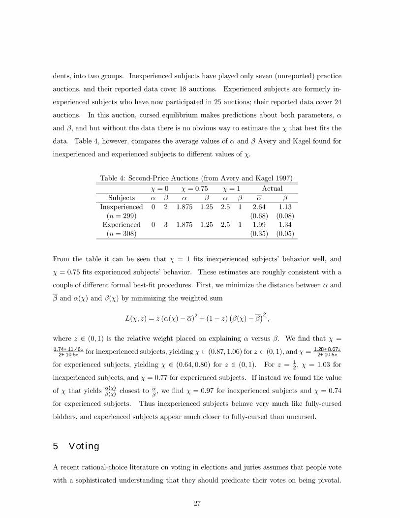
data. Table 4, however, compares the average values of α and β Avery and Kagel found for

inexperienced and experienced subjects to different values of χ.

Table 4: Second-Price Auctions (from Avery and Kagel 1997)

χ = 0 χ = 0.75 χ = 1 ActualSubjects α β α β α β α β

Inexperienced 0 2 1.875 1.25 2.5 1 2.64 1.13(n = 299) (0.68) (0.08)Experienced 0 3 1.875 1.25 2.5 1 1.99 1.34(n = 308) (0.35) (0.05)

From the table it can be seen that χ = 1 Þts inexperienced subjects behavior well, and

χ = 0.75 Þts experienced subjects behavior. These estimates are roughly consistent with a

couple of different formal best-Þt procedures. First, we minimize the distance between α and

β and α(χ) and β(χ) by minimizing the weighted sum

L(χ, z) = z (α(χ)− α)2 + (1− z) ¡β(χ)− β¢2,

where z ∈ (0, 1) is the relative weight placed on explaining α versus β. We Þnd that χ =1.74+11.46z

2+10.5z for inexperienced subjects, yielding χ ∈ (0.87, 1.06) for z ∈ (0, 1), and χ = 1.28+8.67z2+10.5z

for experienced subjects, yielding χ ∈ (0.64, 0.80) for z ∈ (0, 1). For z = 12 , χ = 1.03 for

inexperienced subjects, and χ = 0.77 for experienced subjects. If instead we found the value

of χ that yields α(χ)β(χ)

closest to αβ, we Þnd χ = 0.97 for inexperienced subjects and χ = 0.74

for experienced subjects. Thus inexperienced subjects behave very much like fully-cursed

bidders, and experienced subjects appear much closer to fully-cursed than uncursed.

5 Voting

A recent rational-choice literature on voting in elections and juries assumes that people vote

with a sophisticated understanding that they should predicate their votes on being pivotal.

27

Because a voters vote only matters when she is pivotal, she should vote as if she is pivotal,

even when she suspects that she is not.23 Being pivotal can affect a voters preferences if she

believes that other voters have private information about the proper way to vote, information

that is revealed from the fact that she is pivotal. Hence, a sophisticated voter asks herself

what information other voters would have to make her pivotal, and then how she wants to

vote when she combines that information with her own private information.

In a series of papers, Feddersen and Pesendorfer (1996, 1997, 1998) explore the implications

of such sophisticated reasoning by voters. Feddersen and Pesendorfer (1996) study a variant

of this reasoning in which uninformed voters strictly prefer abstaining to voting, because they

realize that if they are pivotal they are more likely to decide the election in favor of the wrong

candidate. By analogy to the winners curse in auctions, they label this the swing-voters

curse. The label is apt, since less-than-fully-sophisticated voters may fall prey to such a curse

much as bidders in common-values auctions fall prey to the winners curse. In this section

we apply cursed equilibrium to the model developed in Feddersen and Pesendorfer (1998)

of a jury that must decide whether to convict a defendant of some crime. We discuss some

general implications of cursedness in this model, as well as how our results Þt the Þndings of

McKelveys and Palfreys (1998) experimental test of the model.

A jury of size M ≥ 2 must decide whether to convict some defendant of some crime.

Let ωG be the state of the world where the defendant is guilty, and ωI be the state of the

world where the defendant is innocent, and suppose that jurors share the common prior

µ(ωG) = µ(ωI) =12 . Juror k receives a private signal sk ∈ γ, ι, correlated with the state

of the world, with Pr [γ|ωG] = Pr [ι|ωI ] = θ ∈¡

12 , 1¢. Signals are independent conditional on

the state of the world. Each juror k chooses an action ak ∈ g, i, where g is a guilty voteand i an innocent vote. Let σk : γ, ι→4g, i be ks strategy, which maps her signal to aprobability distribution over guilty and innocent votes. Let nG denote the number of jurors

who vote guilty, n−iG denote the number of jurors j 6= i who vote guilty, and nI = M − nGdenote the number of jurors who vote innocent. Let a ∈ A,C be the outcome of the juryprocess, where A denotes acquit and C convict. The voting rule determines how the outcome

depends on the jurors votes. Under unanimous voting, the defendant is convicted if nG =M ;

under majority voting, he is convicted if nG > nI . More generally, let N ∈ £M2 ,M¤ be the23 See Razin (2000) for a version of the sophisticated-voter model when voters care not just about who wins

an election, but also about the margin of victory.

28

number of guilty votes needed to convict the defendant, so that the defendant is convicted if

nG ≥ N.All jurors share the preferences

u(a|ωG) =½q − 1 a = A0 a = C

and u(a|ωI) =½0 a = A−q a = C,

where q ∈ (0, 1) is a parameter measuring the voters trade-offs associated with either con-victing the innocent and acquitting the guilty. The higher q, the more jurors are bothered

by convicting an innocent defendant relative to acquitting a guilty defendant. A juror prefers

to convict if and only if she thinks the probability that the defendant is guilty exceeds q.

Given that the two states, ωG and ωI , are equally likely, and that each private signal

reßects the true state with probability θ > 12 , a juror believes that the defendant is guilty

with probability θ when her signal is γ and with probability 1 − θ when her signal is ι. Weshall assume throughout that 1− θ < q, so that a juror who receives an innocent signal nevervotes to convict based on her information alone. In many applications, we shall consider the

case of q = 12 , so an individual making a decision alone with only one signal would vote to

convict if and only if the signal is guilty.

Because a jurors vote only matters if she is pivotal, it only matters if exactly N −1 otherjurors cast guilty votes. Thus a juror votes to convict if she thinks the probability of the

defendants being guilty is at least q given her own signal and the event that N − 1 otherjurors vote guilty. To Þnd a symmetric equilibrium, consider the strategy σk, where

σk(ak = g|sk) =½1 sk = γσ sk = ι

,

where σ ∈ [0, 1). Under strategy σk, Juror k votes guilty with probability one when she

receives a guilty signal, and votes guilty with probability σ when she receives an innocent

signal. Feddersen and Pesendorfer show a symmetric Bayesian Nash equilibrium of this form

always exists. Of particular note is that the equilibrium often involves σ > 0, so that people

with an innocent signal vote guilty with positive probability. To see why this leads to σ > 0,

note for instance that when NM > θ voters realize that even when the person is guilty they

typically will not convict him based on guilty votes alone; if all those with innocent signals

were to vote innocent, then a person with one of those innocent signals should realize that if

she is pivotal it is almost surely the case that the defendant is guilty. More generally, when

q is low and NM is high, proper voting requires some of those with innocent signals to vote

guilty.

29

In order for there to be a mixed-strategy χ-cursed equilibrium of the form described above

with σ ∈ (0, 1), a juror must be indifferent between voting guilty and innocent when she getsa ι signal. The expected utilities for Juror i with an innocent signal, ι, from each of her two

possible votes are

u(g|ι) = Pr£n−iG 6= N − 1 | ι¤ · u(g | n−iG 6= N − 1) + Pr £n−iG = N − 1 | ι¤ · Vg(σ)

u(i|ι) = Pr£n−iG 6= N − 1 | ι¤ · u(i | n−iG 6= N − 1) + Pr £n−iG = N − 1 | ι¤ · Vi(σ),

where Vg(σ) and Vi(σ) are the jurors perceived payoffs from voting guilty or innocent if she

is pivotal and receives an innocent signal. Because u(g | n−iG 6= N − 1) = u(i | n−iG 6= N − 1) a voter only cares about her vote when it is pivotal u(g | ι) = u(i | ι) if and only ifVg(σ) = Vi(σ). From this,

σ∗ = max½0,θz − (1− θ)θ− (1− θ)z

¾, where z =

µ1− q − θχq − (1− θ)χ

¶ 1N−1

µ1− θθ

¶M−N+1N−1

.24

When θ > 12 and q ≥ 1

2 , σ∗ > 0 if

χ <1− q − ¡1−θ

θ

¢2N−M+2

θ− ¡1−θθ

¢2N−M+3,

and σ∗ = 0 otherwise.

That is, when χ is small, then those with innocent signals vote guilty with positive proba-

bility when N is close enough toM , just as Feddersen and Pesendorfer found. More generally,

cursed equilibrium shares many features of Bayesian Nash equilibrium. For example, when χ

is sufficiently small, jurors with innocent signals sometimes vote guilty. Various comparative

statics hold irrespective of χ. For all χ, ∂σ∗

∂q ≤ 0, meaning that the higher the burden of proofthe jurors need to convict the less likely they are to vote guilty. For all χ, ∂σ

∗∂N ≥ 0, meaning

24To determine the equilibrium values of Vg(σ) and Vi(σ), we Þrst deÞne

A(σ) = Prhι, n−iG = N − 1 | ωG

i=

ÃM − 1N − 1

!(θ + (1− θ)σ)N−1((1− θ)(1− σ))M−N (1− θ)

B(σ) = Prhι, n−iG = N − 1 | ωI

i=

ÃM − 1N − 1

!((1− θ) + θσ)N−1((θ(1− σ))M−Nθ,

the probability that Juror i receives an innocent signal and is pivotal in the guilty and innocent states,respectively. A cursed juror with an innocent signal who knows she is pivotal believes that the defendant isguilty with probability Pg ≡ (1−χ) A(σ)

A(σ)+B(σ)+χ(1−θ) and innocent with probability Pi ≡ (1−χ) B(σ)

A(σ)+B(σ)+

χθ. By observing that Vg(σ) = Pi · (−q) and Vi(σ) = Pg · (q − 1), Vg(σ) = Vi(σ), we get the result presentedin the text.

30

that the higher the number of guilty votes needed to convict, the more likely the jurors are

to vote guilty.

Although partially-cursed jurors may vote strategically, they underinfer one anothers in-

formation when they condition their votes on being pivotal. This affects their voting strategy,

and hence the extent to which voting is efficient the likelihood that an innocent defendant

is acquitted and a guilty defendant convicted. The formula above shows that ∂σ∗

∂χ ≤ 0, mean-ing that the more cursed are jurors, the less likely are jurors with innocent signals to vote

guilty. Because cursed jurors are less inclined to infer from the fact that they are pivotal that

others have received guilty signals, cursedness causes jurors with innocent signals to be more

likely to vote innocent. Indeed, when χ = 1, voters simply vote their signals.

One of the striking results in Feddersen and Pesendorfer (1998) is that Þxing the number

of jurors, M , the probability of convicting an innocent person may increase as the number of

guilty votes needed for conviction, N, increases; this is because the probability with which a

juror with an innocent signal votes guilty may increase so much in response to a higherN that

the odds of convicting an innocent defendant increase. Cursedness mitigates this connection.

While increasing N can raise the probability of conviction even when χ > 0, it decreases the

probability of conviction for χ sufficiently close to 1 because in that case jurors with innocent

signals always vote innocent irrespective of N .

Feddersen and Pesendorfer (1998) characterize the likelihood of acquitting a guilty de-

fendant and convicting an innocent defendant under the unanimity rule when the size of

the jury becomes arbitrarily large. Under the unanimity rule, an innocent defendant is con-

victed with probability Pr [C|ωI ] = [(1− θ) + θσ∗]M and a guilty defendant with Pr [A|ωG] =1− [(1− θ) + θσ∗]M . When χ < 1−q

θ ,

limM=N→∞

Pr [C|ωI ] =

µ(1− q)(1− θ)− θ(1− θ)χ

qθ− θ(1− θ)χ¶ θ

2θ−1

limM=N→∞

Pr [A|ωG] = 1−µ(1− q)(1− θ)− θ(1− θ)χ

qθ − θ(1− θ)χ¶ 1−θ

2θ−1

.

Pr [C|ωI ] is decreasing in χ, and Pr [A|ωG] is increasing in χ: cursedness decreases the proba-bility of convicting an innocent defendant and increases the probability of acquitting a guilty

defendant. When χ > 1−qθ , Pr [C|ωI ] = 0 and Pr [A|ωG] = 1; that is, sufficiently cursed jurors

31

vote their signals, so the defendant is never convicted.25

While in the context of juries comparing unanimity rules to majority rules is natural, in

large-scale elections it is of greater interest to compare intermediate cases where the share of

votes needed to pass a proposition or elect a candidate is between one half and one. While

winning an election typically requires a majority of votes, passing a proposition often requires

a supermajority such as 23 .26 To consider the role of cursedness in such contexts, we consider

the limit as M becomes very large and when N = kM, where k > 12 is a Þxed parameter

representing the percentage of guilty votes needed to convict. In this case,

limM→∞,N=kM

σ∗ =

(1−θ

θ )1−kk − 1−θ

θ

1−( 1−θθ )

1k

for χ < 1−qθ

0 for χ > 1−qθ .

When χ < 1−qθ , neither χ nor q affects the equilibrium proportion of guilty votes in the

limit.27 But both χ and q help to determine whether there is a mixed-strategy equilibrium

in which voters with innocent signals sometimes vote guilty. Indeed, in the limit for k < 1,

the election is fully efficient always acquitting the innocent and convicting the guilty if

and only if the above mixed-strategy equilibrium exists. If the defendant is guilty, proportion

θ+ (1− θ)σ∗ of voters vote guilty, and if the defendant is innocent, proportion (1− θ) + θσ∗

vote guilty. Voting is efficient when (1 − θ) + θσ∗ < k < θ + (1 − θ)σ∗. This holds for all25When χ = 0, limM=N→∞ Pr [C|ωI ] =

³(1−q)(1−θ)

qθ

´ θ2θ−1

and limM=N→∞ Pr [A|ωG] = 1 −³(1−q)(1−θ)

qθ

´ 1−θ2θ−1

, which coincides with the results in Feddersen and Pesendorfer (1998).26 In a multi-candidate race with only two viable candidates, requiring a majority to avoid a run-off amounts

de facto to requiring a super-majority.27The intuition for this independence from χ and q depends on the fact that in a mixed-strategy equilibrium

a voter must be indifferent between voting innocent and voting guilty when she is pivotal and has an innocentsignal. Recall from an earlier footnote that a cursed voter with an innocent signal who knows he is pivotalbelieves that the defendant is guilty with probability Pg ≡ (1 − χ) A(σ)

A(σ)+B(σ)+ χ(1 − θ) and innocent with

probability Pi ≡ (1 − χ) B(σ)A(σ)+B(σ)

+ χθ , where A(σ) and B(σ) are the actual probabilities that a voterreceives an innocent signal and is pivotal in the two states. Since the voter is indifferent between voting guiltyand innocent only if Pi · (−q) = Pg · (q − 1), these equations imply that σ must be such that A(σ)

B(σ)∈ (0, 1).

Intuitively, if the voters perceived probabilities and, hence, the actual probabilities of the two stateswere not of the same order of magnitude, then she would strictly prefer voting innocent or to guilty. BecauseA(σ)B(σ)

=hθ+(1−θ)σ(1−θ)+θσ

ikM−1 h(1−θ)θ

i(1−k)M+1

,

limN≡kM→∞

A(σ)

B(σ)= lim

N≡kM→∞

"µθ + (1− θ)σ(1− θ) + θσ

¶k µ(1− θ)θ

¶(1−k)#M

.

That is, A(σ)B(σ) is a likelihood function describing the relative probability that a voter with an innocent signal

is pivotal in each of the two states; if the fraction being raised to the power M does not equal 1, then in thelimit A(σ)

B(σ)is either inÞnite or zero. In fact, σ∗ is the value of σ that such that limN=kM→∞

A(σ)B(σ)

= 1.

32

values of θ > 12 and k < 1 when χ <

1−qθ .

28 Note that 1−θ < k < θ holds even when σ∗ = 0 ifθ > k. That is, if a higher percentage of voters get guilty signals than are needed to convict,

guilty votes by those with innocent signals are needed.

Given that whether σ∗ > 0 is the sole determinant when k > θ of whether voting in large

elections will be efficient, it is of special note that the condition for σ∗ depends on χ but does

not depend on k. Since χ = 0 always guarantees that σ∗ > 0 when k > θ, this means that

any threshold election rule is efficient for large elections when voters are sufficiently uncursed.

When χ > 1−qθ , by contrast, the election rule is efficient if and only if θ > k >

12 ; that is, the

only election rules that guarantee efficiency for sufficiently cursed voters require conviction

when voters vote naively.

A general principle is that voting mechanisms matter more for cursed than uncursed voters.

Uncursed voters vote in a sophisticated manner by adjusting their behavior to whatever

mechanism they face to assure as best they can that voting is efficient. By contrast, very

cursed voters who vote based on their private information alone do not adjust their behavior

to the mechanism to achieve efficiency. An efficient mechanism with cursed voters, therefore,

needs to implement the right choice when voters vote naively. This suggests, in turn, that

an efficient voting mechanism exists whenever there is a sufficiently large number of voters

whose naive preferences depend on their private signals, so that aggregate voting behavior

depends on whether the true state is that the defendant is guilty or innocent.

The only experimental test of the Feddersen and Pesendorfer model of which we are aware

is McKelvey and Palfrey (1998), who study the laboratory behavior of students at Cal Tech.

Subjects were assigned randomly to groups with either 3 or 6 members. Each group was

assigned with equal probability to one of two urns, the innocent urn with 7 innocent balls

and three guilty balls, or the guilty urn with 3 innocent balls and 7 guilty balls.29 Subjects

did not know to which urn their group had been assigned, but each subject privately and

independently drew a ball at random (sequentially with replacement) from her groups urn.

After observing her ball, each subject voted either innocent or guilty. McKelvey and Palfreys

experiment corresponds to parameter values of µ(ωG) = µ(ωI) = .5, q = .5, and θ = .7 in the

model outlined above. Different groups faced different rules determining how their votes were

28This can be proven by noting that when θ = 1, (1− θ) + θσ∗ = 0 and θ + (1 − θ)σ∗ = 1, and that whenθ & 1

2, (1 − θ) + θσ∗ = θ + (1 − θ)σ∗ = k. The result is then established by showing that (1 − θ) + θσ∗ is

strictly decreasing in θ and θ + (1− θ)σ∗ is strictly increasing.29We follow the authors in using the langauge of guilty and innocent in describing the experiment,

although the actual states described to the subjects were the more neutral terms Red and Blue.

33

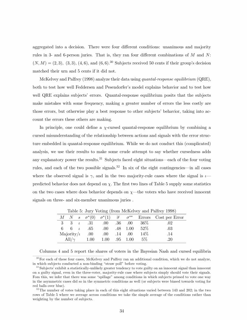
aggregated into a decision. There were four different conditions: unanimous and majority

rules in 3- and 6-person juries. That is, they ran four different combinations of M and N :

(N,M) = (2, 3), (3, 3), (4, 6), and (6, 6).30 Subjects received 50 cents if their groups decision

matched their urn and 5 cents if it did not.

McKelvey and Palfrey (1998) analyze their data using quantal-response equilibrium (QRE),

both to test how well Feddersen and Pesendorfers model explains behavior and to test how

well QRE explains subjects errors. Quantal-response equilibrium posits that the subjects

make mistakes with some frequency, making a greater number of errors the less costly are

those errors, but otherwise play a best response to other subjects behavior, taking into ac-

count the errors these others are making.

In principle, one could deÞne a χ-cursed quantal-response equilibrium by combining a

cursed misunderstanding of the relationship between actions and signals with the error struc-

ture embedded in quantal-response equilibrium. While we do not conduct this (complicated)

analysis, we use their results to make some crude attempt to say whether cursedness adds

any explanatory power the results.31 Subjects faced eight situationseach of the four voting

rules, and each of the two possible signals.32 In six of the eight contingenciesin all cases

where the observed signal is γ, and in the two majority-rule cases where the signal is ι

predicted behavior does not depend on χ. The Þrst two lines of Table 5 supply some statistics

on the two cases where does behavior depends on χthe voters who have received innocent

signals on three- and six-member unanimous juries .

Table 5: Jury Voting (from McKelvey and Palfrey 1998)

M N s σ∗(0) σ∗(1) σ σ∗∗ Errors Cost per Error3 3 ι .31 .00 .36 .00 36% .026 6 ι .65 .00 .48 1.00 52% .03Majority/ι .00 .00 .14 .00 14% .14All/γ 1.00 1.00 .95 1.00 5% .20

Columns 4 and 5 report the shares of voters in the Bayesian Nash and cursed equilibria30For each of these four cases, McKelvey and Palfrey ran an additional condition, which we do not analyze,

in which subjects conducted a non-binding straw poll before voting.31Subjects exhibit a statistically-unlikely greater tendency to vote guilty on an innocent signal than innocent

on a guilty signal, even in the three-voter, majority-rule case where subjects simply should vote their signals.Fom this, we infer that there was some spillage among conditions in which subjects primed to vote one wayin the asymmetric cases did so in the symmetric conditions as well (or subjects were biased towards voting forred balls over blue).32The number of votes taking place in each of this eight situations varied between 143 and 202; in the two

rows of Table 5 where we average across conditions we take the simple average of the conditions rather thanweighting by the number of subjects.

34

who should vote guilty, and Column 6 shows the percentage of subjects, σ, who actually voted

guilty. As can be seen, too many people voted guilty in the three-person anonymous casethe

opposite of the error predicted by cursedness. On the other hand, too few people voted guilty

in the six-person unanimous case, consistent with cursedness. Column 7 indicates how each

individual subject should have voted had she known how others were voting. Given that too

many subjects voted guilty in the three-person case, the optimal strategy for an individual

voter would be to vote innocent for sure; given that too many were voting innocent in the

six-person case, the optimal strategy would be to vote guilty for sure. Hence, Column 7 shows

that 36% of subjects were voting erroneously in the direction opposite of cursedness in the

three-person case, and 52% of subjects were voting erroneously in the direction predicted by

cursedness in the six-person case, suggesting that subjects were more prone to cursed errors

than uncursed errors. For further comparison, the third row of Table 5 lists together the

other two innocent-signal conditions, indicating that only 14% of subjects make errors in

these cases. The fourth row shows average behavior by subjects getting guilty signals in the

four conditions, indicating that only 5% of subjects vote incorrectly in these cases.

Subjects make more errors in the one case where those errors are cursed than in any

other case. However, these error rates is complicated by the fact that some errors are costlier

than others. Column 9 shows the expected cost of each error, measured in terms of how much

each error lowers the expected likelihood of reaching the correct verdict. Since the expected

cost of voting incorrectly in the conditions represented in the last two rows is much higher

than in the Þrst two conditions, the lower number of errors may merely reßect their costliness

rather than the uncursed nature of the error. Yet the expected cost of voting innocent in the

six-person case is greater than the expected cost of those voting guilty in the three-person

case, which suggests that the greater number of these cursed errors cannot be fully explained

by their low cost.33

An alternative method of estimating subjects cursedness in this experiment is by com-

puting the maximum-likelihood estimate of χ under the maintained hypothesis that almost

nobody makes any error except cursedness. In this case, the huge number of subjects voting in-

correctly in the six cases where cursedness should not affect behavior are merely ßukes, and

we look for the χ that best Þts subjects behavior in the two cases where the mixed-strategy

33 If instead we compared the expected cost of the error conditional on being pivotal, the difference wouldbe more dramatic: 19% vs. 6%, rather than 3% vs. 2%.

35

played depends on χ. In this case, the maximum-likelihood value of χ is .10.34 Because neither

method of estimating χ is very satisfying, and neither method yields a very high estimate

of χ, we conclude that whatever support McKelvey and Palfreys voting data provide for

cursedness is very weak.

6 Signaling

In this section, we brießy apply cursed equilibrium to two different signaling contexts, starting

with classical simple signaling games. Because it causes the receiver to infer less from signals

than she should, it is natural to suppose that cursedness may make a high-quality type of

sender unable to separate herself from a low-quality type by sending a costly signal, and hence

unwilling to send the signal. This intuition is not, however, always valid: because a cursed

receiver does not fully infer that a sender who does not send a costly signal is a low type,

cursedness may make a low type of sender less desperate to mimic a high type and hence

make the high type able and willing to reveal herself by sending a costly signal.

To illustrate this, consider a situation where a sender is with equal probability one of two

types, t = b, (bad) and t = g (good). After learning her type, the sender can send one

of two signals, e = l (low) and e = h (high). A receiver infers the senders type from her

signal, where epl and eph represent the receivers beliefs about the probability that the senderis type g following signals l and h. After observing the signal the receiver chooses an action

a ∈ [0, 1] and has utility function u(a, g) = −(1− a)2 and u(a, b) = −a2.35 Hence, a receiver

with beliefs ep about the senders type maximizes his expected utility −ep(1−a)2−(1− ep)a2 by

choosing a = epl and a = eph following signals e = l and e = h.We assume that there is a continuous, increasing function f : R → R and real numbers

cb > cg > 0 such that (presented in reduced form that integrates the receivers optimal

response of a = ep) ub = ug = f(epl) is the payoff to both types of sender if the signal l issent, while ub = f(eph)− cb and ug = f(eph)− cg are the payoffs to the bad and good types ofsender, respectively, if the signal h is sent. Thus, both types of sender want the receiver to

34This solves the maximum-likelihood from the observed data in these two cases:maxχ L(χ) ≡

¡18667

¢(σ∗(M = N = 3,χ))67 (1− σ∗(M = N = 3,χ))121 ·¡

18689

¢(σ∗(M = N = 6,χ))89 (1− σ∗(M = N = 6,χ))97

35The action a can be thought of as an investment that the receiver Þnds attractive if the sender is a goodtype but unattractive if he is a bad type.

36

believe that she is the good type; the signal h can potentially serve as a signal because it is

more costly for the bad type than for the good type.

Because cb > cg, any separating Bayesian Nash equilibrium must involve type g sending

signal h and type b sending l. For a separating equilibrium to exist, the good type must

prefer to send h, so that f(1) − cg ≥ f (0), and the bad type must prefer to send l, so

that f(1) − cb ≤ f(0). Hence, a separating Bayesian Nash equilibrium exists if and only if

cg ≤ f(1)− f(0) ≤ cb.When is there a separating χ-cursed equilibrium? In a separating equilibrium, because a

χ-cursed receiver believes that type g sends h with probability 1− χ2 and type b sends h with

probability χ2 , he forms the beliefs epl = χ

2 and eph = 1 − χ2 . Hence, a separating χ-cursed

equilibrium exists if and only if cg ≤ f(1− χ2 )− f(χ2 ) ≤ cb. When χ = 1, f

¡1− χ

2

¢− f ¡χ2 ¢ =f¡

12

¢−f ¡12

¢= 0, so that no signaling can occur when the receiver is fully cursed. Intuitively,

no sender would send a costly signal that would not affect the receivers beliefs.36

While fully-cursed receivers always destroy the potential for signaling, however, less ex-

treme cursedness can create the potential for successful signaling. Indeed, if cb < f(1)−f(0),so that no separation can occur in a Bayesian Nash equilibrium, then because f

¡1− χ

2

¢−f ¡χ2 ¢is decreasing in χ, there is some χ ∈ (0, 1) such that there is a separating cursed equilibrium.Intuitively, if the cost of being identiÞed as the bad type is so high that the bad type prefers

sending the costly signal to being identiÞed, then full separation is not compatible with

Bayesian Nash equilibrium. If the receiver is cursed enough that the bad type is just barely

willing to behave differently than the good type, then the good type will be willing to reveal

herself.

We now turn to an example of signaling that we call a the revelation game, modeled

after politicians who feel constrained not to lie to voters, but who do not feel constrained

to reveal the full truth. In the 1999-2000 American presidential campaign, candidate George

W. Bush has said that he has never had an extramarital affair, and that he has not used

cocaine in the past 25 years. But he refuses to say whether he used cocaine more than 25

years ago. Especially since Governor Bush volunteered the precise number 25, fully rational

voters probably should infer that Governor Bush used cocaine 26 years ago. But what would

cursed voters infer from his (non)report?

36While a separating Bayesian Nash equilibrium may not be a separating cursed equilibrium, recall thatProposition 3 demonstrates that every pooling Bayesian Nash equilibrium is a pooling χ-cursed equilibrium,for every value of χ.

37

Suppose a sender is of some type t ∈ [0, 1], where t is a measure of her age the last timeshe engaged in some unseemly activity. A receiver does not know t, but has uniform priors

on [0, 1]. The sender chooses a message m ∈ [0, 1] ∪ S: she either announces that she issome type in [0, 1] or chooses S, meaning she remains silent. After observing the senders

message, the receiver forms beliefs about the senders type; let Pm(t) be the receivers beliefs

about the probability that the senders type is less than t following the message m. We

assume that the receiver picks an action a(m) ∈ [0, 1] to maximize the expectation of hispayoff −(a(m)− t)2. This means that the receiver chooses the action that coincides with hisexpectation of the senders type given her message. The type t of senders payoffs are −a(m)if m ∈ t, S and −a(m)− c if m /∈ t, S. Hence, she wants the receivers beliefs to be as lowas possible, but she pays a cost of c if she misreports her type. We assume that c > 1, so no

sender ever has incentive to misreport her type.

The most plausible Bayesian Nash equilibrium in this game is that all types reveal them-

selves fully.37 What are the cursed equilibria? Suppose the sender follows the cutoff strategy

r ∈ [0, 1], revealing her type iff t < r. A χ-cursed receiver forms beliefs χ12+(1−χ)

¡12 +

r2

¢=

12 +(1−χ) r2 , so the sender prefers to reveal whenever t < 1

2+(1−χ) r2 . Because the marginaltype r must be indifferent between revealing and not revealing, r = 1

2 + (1 − χ) r2 , whichimplies r = 1

1+χ . Such a cutoff strategy is optimal for the sender, since types t < r prefer

revealing, while types t > r prefer pooling.

When χ = 0, r = 1, and all types reveal. The intuition is familiar: the lowest type

always prefers to reveal herself. If only the lowest types reveal, then the lowest types who are

supposed to pool will also prefer revealing, since they will have types lower than the average

of all pooling types. For χ > 0, however, some types pool. Because the receiver mistakenly

believes that some types of sender who reveal pool, and that some types of sender who pool

reveal, when the receiver sees a sender who refuses to reveal her type he thinks that she has

37 In fact, if we deÞned the game such that the sender cannot misreport her type, then this would be theunique perfect Bayesian equilibrium. But because we have not deÞned cursed equilibrium for games wherea players action space depends on her type, we could not apply cursed equilibrium to this game. In theconclusion, we discuss some of the problems that accompany cursed equilibrium in such games. In the gameas we have deÞned it, there are other perfect Bayesian equilibria. One is that each type of sender chooses theaction S, and the receiver chooses a(S) = 1

2and a(m) = 1 for m 6= S. In this equilibrium, no sender reveals

her type because the receiver punishes any announcement of the senders types with the extreme actiona = 1. This strategy does not survive other reÞnements such as iterated weak dominance or the intuitivecriterionthe receiver should not beleive that the message m could be sent by any type of sender other thant = m since any other type t0 6= m could do better by announcing either m = t0 or m = S, whatever thereceivers continuation strategy.

38

a lower type than she actually does.

We conclude with an experiment by Forsythe, Isaac, and Palfrey (1989) that provides

some evidence for cursedness in a game very similar to the revelation game. Their game is

inspired by the American Þlm industry, where movie distributors auction the rights to show

Þlms to movie-theater operators. Forsythe, Isaac, and Palfrey report that over 90% of Þlms

are auctioned off before they are shot. Theater owners dislike this practice, possibly because

they suffer a winners curse on movies auctioned before being shot. Distributors privately

informed about the quality of their Þlms pre-production who are obliged to reveal quality

post-production may auction off bad movies before production and good ones after, much

as in the revelation game good types reveal while bad types conceal. In Forsythe, Isaac and

Palfreys (1989) experiment, each of four sellers was endowed with one unit of an object whose

common value (in cents) to each of four bidders was drawn from a uniform distribution on

1, 2, ..., 125. Each seller knew the value of her object, but the bidders did not. The sellerschose whether to reveal the value of their objects to the bidders or conceal them; a seller who

revealed her value had to do so truthfully. Following this, the objects were auctioned to the

bidders using Þrst-price auctions, where each buyer bid on each of the sellers items. Just

as in the revelation game, there is a cutoff χ-cursed equilibrium where sellers with objects

valued more than r = 125χ+11+χ reveal their values, while sellers with objects valued less than

r = 125χ+11+χ conceal their values. Intuitively, low-value sellers conceal the value of their objects

because cursed bidders mistakenly think that some high-value sellers conceal, causing them to

bid too high for objects whose values are concealed. When χ = 0, all sellers (except possibly

ones with the lowest possible valuation) reveal. When χ = 1, sellers with valuations under

63 conceal, and those with valuations above 63 reveal. Each bidder bids her expectation of

the valuation of each sellers object, which is r for those sellers who conceal.

Forsythe, Isaac, and Palfrey ran 60 trials of this experiments with three groups of under-

graduate subjects; the Þrst group participated in 16 trials, and the second and third groups

participated in 22 trials. Table 6 summarizes the data.

Table 6: Revelation Game (from Forsythe, Isaac, and Palfrey 1989)

Group Sellers Conceal Value Conceal Bid Conceal χ

All 240 85 31 39 0.44Experienced 120 32 23 27 0.27Experienced* 72 12 11 19 0.17

39

The Þrst row of the table shows the data for all sellers. For objects whose value was

revealed, the winning bid was always approximately equal to the value of the object. Columns

2 and 3 show that 85 of 240 sellers (35%) concealed the value of their objects. For sellers

who concealed, the average value of their objects was 31, but the average winning bid was

39. Hence buyers suffered a winners curse, paying an average of 8 cents more than the

value of the objects they won. There are two natural ways to estimate χ from the data,

one from the average winning bid and one from the average value of the objects concealed.

Consider the data from the Þrst row and suppose that the sellers follow a cutoff strategy

revealing when their values were high and concealing otherwise. Then because the average

value of the sellers objects is 31, sellers would be revealing when their objects were worth

more than 61 and concealing otherwise. Then since in equilibrium 61 = r = 125+χ1+χ , χ ' 0.83;

that is, sellers who thought that bidders were cursed with χ = 0.83 would reveal with values

over 61 and conceal otherwise. If sellers were following this strategy, however, then cursed

bidders would bid an average of 61, far more than the 39 that they actually bid. The other

method of estimating χ is to assume that cursed bidders believe that sellers follow a cutoff

strategy, and estimate χ from the average winning bid. In this case, χ ' 0.44. In Table

6, we present estimates of χ using the second of these methods since it corresponds better

to bidder behavior as well as to seller behavior with the notable exception of a few outlying

high-value objects whose values were concealed in early rounds of the experiment: 68 of 88

sellers (77%) with values less than 39 concealed , and 17 of 152 (11%) of sellers with values

more that 39 concealed; by contrast, only 74 of the 128 (58%) of the sellers with values less

than 61 and 11 of the 112 (10%) sellers with values greater than 61 concealed. Thus, given

bidders behavior, 37 of 240 sellers (15%) made mistakes: the 20 with objects worth less than

39 who revealed, and the 17 with objects worth more than 39 who concealed. In other words,

those sellers whose objects were worth less than 39 and revealed had objects with signiÞcantly

higher valuations than those sellers with objects worth less than 39 who concealed.38

38 In fact, seller behavior is better described by a simple step rule: sellers with the lowest valued concealed;sellers with intermediate values conealed half of the time; and sellers with high values revealed. 43 of 44 sellerswith objects valued less than 25 concealed, and the average value of their objects was 14; the value of theobject of the lone seller who revealed was 16. 31 of 58 sellers (53%) with values between 25 and 49 concealed,and the average value of their objects was 34; the average value of the 27 who revealed was 36. Finally, 11 ofthe 138 sellers (8%) with objects worth at least 50 concealed (8%), and the average value of their objects was88; the average value of the 127 who revealed was 86. The fact that within each of these groups the averagevalue of the objects of sellers who concealed roughly equals the average value of the objects of those sellerswho revealed suggests that sellers decisions to reveal did not depend on their objects values.

40

The second row of the table describes only those subjects who have already participated

in 10 trials or more trials 11 to 16 for the one group that participated in 16 trials, and

trials 11 to 22 for the other two groups. 27 percent of sellers concealed the value of their

objects; the average value of these sellers objects was 23, and the average winning bid was

27. Thus even experienced bidders suffered a winners curse, albeit half of what it was in the

aggregate data. Again, if cursed bidders in these Þnal rounds believed that sellers followed a

cutoff strategy, concealing if their value was less than r and revealing otherwise, then from

the data r = 27, so χ ' 0.27. Seller behavior is very close to this as 20 of the 22 sellers (91%)with objects worth 27 or less concealed, and 12 of 98 sellers (12%) of sellers with objects

worth more than 27 concealed.

Finally, because in one of the three groups a single subject won 16 of the 20 of the auctions

where the seller concealed her value, bidding an average of 35, the third row excludes this

subjects group from the pool of experienced subjects. This time, only 17% of sellers concealed

the value of their objects. The winners curse is larger than for experienced subjects, as the

average value of sellers objects was 11, while the average winning bid was 19. Thus the

winners curse was larger. For this group, χ ' 0.17.

7 Discussion and Conclusion

We believe that cursed equilibrium can provide insight in many additional domains. One is in

organizational and sequential decision-making, where we believe that cursedness may capture

a form of exaggerated fear that some parties may have of putting other parties in charge of

decisions, under-appreciating the fact that unanticipated future decisions by others may be

based on unanticipated information. Consider, for instance, a grand jury that must decide

whether to indict some defendant of a crime. If the defendant is indicted, the case proceeds

to trial where a jury hears the evidence and decides whether to convict the defendant. In

this case, a sufficiently cursed grand jury that is not yet convinced of the defendants guilt

may be too reluctant to indict. This is because it fears that the jury will convict when the

defendant is innocent, even though it should realize that the jury only convicts if it has strong

evidence that the defendant is guilty. Similarly, principals in organizations may be reluctant

to delegate decisions even to parties whose interests coincide with their own out of fear that

the these other parties would make different decisions than they would, underappreciating

41

how often those different decisions reßect superior information.39

Many applications of cursed equilibrium point to limitations and problems with the solu-

tion concept as we have deÞned it, and we conclude by discussing some of these shortcomings

and possible extensions of the solution concept. One limitation of cursed equilibrium is that

we have only deÞned it in games where each players action space is independent of her type.

In games without such independence, cursed equilibrium should presumably be deÞned such

that players do not assign positive probability to a type playing an action that is impossible

for that type. A problem with this approach, however, is that a cursed equilibrium in the

game where an action is impossible for a type of a player might differ from a cursed equilib-

rium in the related game where that same action is possible, but strictly dominated, for that

type.

This problem, in turn, suggests a modiÞed deÞnition in which we assumed that no player

thinks that any type of any other player plays a strictly dominated action in equilibrium.

More generally, cursed equilibrium could be revised to incorporate the notion that the worse

an action is for a type, the less likely other players think that type is to take that action.

Developing a new concept incorporating this notion seems important both intuitively and for

practical application, but would raise new problems such as determining how to measure and

compare how irrational a given action is for different types of a player, and precisely how to

restrict beliefs as a function of the degree of irrationality associated with a rule. And the

enterprise would be inherently limited, since the very notion of cursed equilibrium is meant to

capture limits to the degree to which people think through the relationship between others

relevant information and their behavior.

Perhaps a more urgent direction for developing the idea of cursed equilibrium concerns a

more important limitation to our current deÞnition. The notion of cursed equilibrium is meant

to capture a general intuition that people tend to underappreciate the relationship between

39To illustrate with a simple principal-agent model, let Ω = ω1,ω2 be the set of possible states of theworld, where the principal and agent share the common prior µ(ω1) = µ(ω2) =

12 . If the principal invests in

an experiment, the agent learns which is the true state, otherwise the agent learns nothing about the state.Once the agent has received his information, he chooses an action a ∈ a1, a2, a3. The principal and theagent share the common payoffs u(a1,ω1) = u(a2,ω2) = 2, u(a1,ω2) = u(a2,ω1) = −2, and u(a3,ω) = 1 foreach ω. That is, the agent attempts to match action ai to state ωi, while the safe action a3 pays one in eachstate. Then if the agent learns the true state, he matches his action to the state, earning a payoff of 2. Ifthe agent does not learn the state, he chooses a1, earning a payoff of 1. A rational principal therefore prefersthat the agent learn the true state. But if the principal is cursed, her perceived payoff from performing theexperiment is (1− χ)2 + χ ¡ 1

22 + 1

2(−2)¢ = 2(1− χ),which exceeds one only when χ < 1

2. Thus a sufficiently

cursed principal prefers that the agent not learn the true state and hence take the safe action, because sheinnappropriately fears that the risky action following the experiment might mismatch the state.

42

others actions and the information these others have at the time they take those actions. Yet

our formal deÞnition makes an artiÞcial distinction between private information represented

by a type space in a Bayesian game and private information that is not represented by the

type space. In sequential games, for instance, our deÞnition assumes that Player 3 does not

fully appreciate how Player 2s actions depend on Player 2s types, but does fully appreciate

how Player 2s actions depend on any actions that Player 1 might take that Player 2 observes

but Player 3 does not. We hope to move towards a more complete notion of cursed equilibrium

which allows for cursedness over more general types of unobservable information that others

have.40

Many other generalizations of cursed equilibrium seem important to add more realistic

variation in the degree of cursedness in different situations. For instance, we Þnd it intuitive

that players are less likely to ignore the informational content of given actions by other players

when they have not actually observed those actions than when they have; observing actions

seems likely to induce more strategic interpretations. This might imply that the reactions by

players to the observed actions in certain sequential games are less cursed than they would

be in corresponding simultaneous-move games. For example, Dekel and Piccione (2000) show

in a rational model of binary voting that the set of informative equilibria is not affected by

whether voters vote sequentially or simultaneously. While we believe the same equivalence

holds with cursed equilibrium as we have deÞned in this paper, a better model may have a

cursed voter understand the relationship between other voters signals and votes better when

she can observe their votes than when she cannot, leading to more rational voting in the

sequential than in the simultaneous-move voting procedure.

A Þnal generalization of cursed equilibrium, manifestly needed to more tightly Þt the data,

is to allow different players to be cursed to different extents. Such heterogeneity is the natural

interpretation of many of the experiments cited above, for instance; while we believe that in

many cases behavior was usefully characterized by positing a uniform χ > 0 across subjects,

the behavior would be even better described by allowing for heterogeneity.41

40The different treatment of exogenous and endogenous private information seems not only intuitivelyand psychologically wrong to us, but creates some highly artiÞcial differences in predictions based on the waya game is formally written down. In particular, insofar as a Bayesian game where one player has privateinformation can be rewritten as an alternative Bayesian game where a Þctitious player is added who takesactions observable by the privately-informed player, our deÞnition of cursed equilibrium is not robust.41 In fact, we suspect that in some circumstances heterogenous cursedness may lead to some qualitatively-

different predictions than homogenous cursedness.

43

8 Appendix

Proof of Lemma 1 From Bayes Rule,

bptk(t−k|a−k,σ−k) =(1− χ)σ−k(a−k|t−k) + χσ(a−k|tk)P

t0−k∈T−k¡(1− χ)σ−k(a−k|t0−k) + χσ(a−k|t0k)

¢p(t0−k|tk)

p(t−k|tk)

=

µ(1− χ) σ−k(a−k|t−k)

σ(a−k|tk) + χ

¶p(t−k|tk).

Proof of Proposition 1 Consider the alternative game (A,T, p, uχ), where (A,T, p) are all

the same, but u is replaced by

uχk (ak, a−k; tk, t−k) ≡ (1− χ)uk(ak, a−k; tk, t−k) + χ

Xt−k∈T−k

pk(t−k|tk)uk(ak, a−k; tk, t−k).

The utility function of type tk of Player k is the χ-weighted average of her actual utility

function and her average utility function, averaged over all possible types of her opponents.

σ is a Bayesian Nash equilibrium of Gχif for each Player k and each type tk ∈ Tk, and each

a∗k such that σk(a∗k|tk) > 0,

a∗k ∈ arg maxak∈Ak

Xt−k∈T−k

pk(t−k|tk)X

a−k∈A−kσ−k(a−k|t−k)uχk (ak, a−k; tk, t−k)

= (1− χ)X

t−k∈T−kpk(t−k|tk)

Xa−k∈A−k

σ−k(a−k|t−k)uk(ak, a−k; tk, t−k)

+χX

t−k∈T−kpk(t−k|tk)

Xa−k∈A−k

σ−k(a−k|t−k)X

t−k∈T−kpk(t−k|tk)uk(ak, a−k; tk, t−k).

But

χX

t−k∈T−kpk(t−k|tk)

Xa−k∈A−k

σ−k(a−k|t−k)X

t−k∈T−kpk(t−k|tk)uk(ak, a−k; tk, t−k)

= χX

a−k∈A−k

Xt−k∈T−k

pk(t−k|tk)σ−k(a−k|t−k)X

t−k∈T−kpk(t−k|tk)uk(ak, a−k; tk, t−k)

= χX

a−k∈A−k

Xt−k∈T−k

pk(t−k|tk)uk(ak, a−k; tk, t−k)σ−k(a−k|tk)

= χX

t−k∈T−kpk(t−k|tk)

Xa−k∈A−k

σ−k(a−k|tk)uk(ak, a−k; tk, t−k),

and henceXt−k∈T−k

pk(t−k|tk)X

a−k∈A−kσ−k(a−k|t−k)uχk (ak, a−k; tk, t−k) =X

t−k∈T−kpk(t−k|tk)

Xa−k∈Ak

[χσ−k(a−k|tk) + (1− χ)σ−k(a−k|t−k)]uk(ak, a−k; tk, t−k).

44

Thus if σ is a Bayesian Nash equilibrium of Gχ, it is also a cursed equilibrium of G. Because

Gχis Þnite, it has a Bayesian Nash equilibrium, and so G has a cursed equilibrium. ¤

Proof of Proposition 2 If each type tk of each player ks expected payoff from playing ak

when the other players play a−k in the χ-virtual game Gχis independent of χ, then the result

follows since the set of Bayesian Nash equilibria of G0= G coincides with the set of Bayesian

Nash equilibria of Gχ, which by Proposition 1 is the set of χ-cursed equilibria of G. Hence it

suffices to show that Xt−k∈T−k

pk(t−k|tk)uk(ak, a−k; tk, t−k)

=X

t−k∈T−kpk(t−k|tk)

Xt−k∈T−k

pk(t−k|tk)uk(ak, a−k; tk, t−k)

The second expression can be rewrittenXt−k∈T−k

pk(t−k|tk)X

t−0k∈T−0k

pk(t−0k|tk)Xt0∈T0

pk(t0|tk, t−0k)uk(ak, a−k; t0, tk, t−0k)

=X

t−k∈T−kpk(t−k|tk)

Xt0∈T0

pk(t0|tk, t−0k)uk(ak, a−k; t0, tk, t−0k)X

t−0k∈T−0k

pk(t−0k|tk),

since E [uk(ak, a−k; t0, tk, t−0k)|tk, t−0k] is independent of t−0k. Hence, the expression simpli-

Þes to

=X

t−k∈T−kpk(t−k|tk)

Xt0∈T0

pk(t0|tk, t−0k)uk(ak, a−k; t0, tk, t−0k)

=X

t−0k∈T−0k

pk(t−0k|tk)Xt0∈T0

pk(t0|tk, t−0k)uk(ak, a−k; t0, tk, t−0k)

=X

t−k∈T−kpk(t−k|tk)uk(ak, a−k; tk, t−k)

as desired. ¤

Proof of Proposition 3 Suppose that σ is strategy proÞle such that for each Player k there

exists some ak ∈ Ak such for each tk ∈ Tk σ(ak|tk) = 1. Then

σ−k(a−k|tk) ≡X

t−k∈T−kpk(t−k|tk)σ−k(a−k|t−k) = σ−k(a−k|t−k)

Xt−k∈T−k

pk(t−k|tk) = σ−k(a−k|t−k),

since σ−k(a−k|t−k) does not depend on t−k. If σ is a χ-cursed equilibrium, then ak maximizesXt−k∈T−k

pk(t−k|tk) ·X

a−k∈A−k[χσ−k(a−k|tk) + (1− χ)σ−k(a−k|t−k)] uk(ak, a−k; tk, t−k)

=X

t−k∈T−kpk(t−k|tk) ·

Xa−k∈A−k

σ−k(a−k|t−k)uk(ak, a−k; tk, t−k),

45

which does not depend on χ. Therefore, whatever χ, ak maximizes Player ks expected payoff

given that players j 6= k play σ−k(a−k|t−k), so σ is a χ-cursed equilibrium for every χ ∈ [0, 1].¤

46

References

[1] Akerlof, George. The Market for Lemons: Quality Uncertainty and the Market Mech-

anism. Quarterly Journal of Economics 84, August 1970: 488-500.

[2] Athey, Susan. Single Crossing Properties and the Existence of Pure Strategy Equilibria

in Games of Incomplete Information, mimeo February 1997, MIT.

[3] Avery, Christopher and John H. Kagel. Second-Price Auctions with Asymmetric Payoffs:

An Experimental Investigation. Journal of Economics & Management Strategy 6(3), Fall

1997: 573-603.

[4] Ball, Sheryl.B.; Bazerman, Max H.; and John S. Carroll. An Evaluation of Learning in

the Bilateral Winners Curse, Organizational Behavior and Human Decision Processes

48:1-22.

[5] Bazerman, Max H. and William F. Samuelson. I Won the Auction But I Dont Want

the Prize, Journal of Conßict Resolution 27(4), December 1983: 618-634.

[6] Dekel, Eddie and Michele Piccione. Sequential Voting Procedures in Symmetric Binary

Elections, Journal of Political Economy 108(1), February, 2000: 34-55.

[7] Dyer, Douglas Kagel, John H. and Dan Levin. A Comparison of Naive and Experienced

Bidders in Common Value Offer Auctions: A Laboratory Analysis, Economic Journal

99, March 1989: 108-115.

[8] Feddersen, Timothy and Wolfgang Pesendorfer. The Swing Voters Curse, American

Economic Review 86(3), June, 1996: 408-424.

[9] Feddersen, Timothy and Wolfgang Pesendorfer. Voting Behavior and Information Ag-

gregation in Elections with Private Information, Econometrica 65(5), 1997: 1029-1058.

[10] Feddersen, Timothy andWolfgang Pesendorfer. Convicting the Innocent: the Inferiority

of Unanimous Jury Verdicts under Strategic Voting, American Political Science Review,

90(1), 1998: 23-35.

[11] Forsythe, Robert; Isaac, R. Mark; and Thomas R. Palfrey. Theories and Tests of Blind

Bidding in Sealed-Bid Auctions, RAND Journal of Economics 20(2), Summer 1989:

214-238.

47

[12] Garvin, Susan and John H. Kagel. Learning in Common Values Auctions: Some Initial

Observations, Journal of Economic Behavior & Organization 25, 1994: 351-372.

[13] Jacobsen, Ben; Potters, Jan; Schram, Arthur; van Winden, Frans; and Jörgen Wit.

(In)accuracy of a European Political Stock Market: The Inßuence of Common Value

Structures, European Economic Review 44, 2000: 205-230.

[14] Klemperer, Paul. Auction Theory: A Guide to the Literature, Journal of Economic

Surveys 13(3), 1999: 227-260.

[15] Holt, Charles A. and Roger Sherman, The Losers Curse. American Economic Review

84(3), June 1994: 642-652.

[16] Kagel, John H. Auctions: A Survey of Experimental Research, in The Handbook

of Experimental Economics, John H. Kagel and Alvin E. Roth, eds, Princeton NJ:

Princeton University Press: 1995.

[17] Kagel, John H. and Dan Levin. The Winners Curse and Public Information in Common

Value Auctions, American Economic Review, 76(5), December 1986: 894-920.

[18] Levin, Dan; Kagel, John H.; and Jean-Francois Richard. Revenue Effects and Process-

ing in English Common Value Auctions, American Economic Review 86(3), June 1996:

442-460.

[19] Lind, Barry and Charles R. Plott. The Winners Curse: Experiments with Buyers and

Sellers, American Economic Review 81(1), 1991: 335-346.

[20] McKelvey, Richard D. and Thomas R. Palfrey. An Experimental Study of Jury Deci-

sions. Mimeo, California Institute of Technology, July 2, 1998.

[21] Milgrom, Paul and John Roberts. Rationalizability, Learning, and Equilibrium in

Games with Strategic Complementarities, Econometrica 58(6), November 1990: 1255-

1277.

[22] Milgrom, Paul and Nancy Stokey. Information, Trade, and Common Knowledge,

Journal of Economic Theory 26: 17-27.

[23] Milgrom, Paul R. and Robert J. Weber. A Theory of Auctions and Competitive Bid-

ding. Econometrica 50(5), September 1982: 1089-1122.

48

[24] Potters, Jan and Jörgen Wit. Bets and Bids: Favorite-Longshot Bias and Winners

Curse, CentER Discussion Paper 9604, Tilburg University, June 1995.

[25] Razin, Ronny. Swing Voters and Mandate Makers: Voting when Margin of Victory

Matters, Mimeo, Princeton University, April 1999.

[26] Samuelson, William F. and Bazerman, Max H. TheWinners Curse in Bilateral Negotia-

tions. In Research in Experimental Economics, vol. 3, Vernon L. Smith, ed., Greenwich,

CT: JAI Press, 1985.

[27] Thaler, Richard H. The Winners Curse, Journal of Economic Perspectives 2(1),

1988:191-202.

49