Embed Size (px)
Citation preview
Currency Hedging in Emerging Markets: Managing Cash Flow Exposure Laura Alfaro Mauricio Calani Liliana Varela
Working Paper 21-096
Working Paper 21-096
Copyright © 2021 Laura Alfaro, Mauricio Calani, and Liliana Varela.
Working papers are in draft form. This working paper is distributed for purposes of comment and discussion only. It may not be reproduced without permission of the copyright holder. Copies of working papers are available from the author.
Funding for this research was provided in part by Harvard Business School. The opinions expressed in paper do not represent those of the Board of the Central Bank of Chile.
Currency Hedging in Emerging Markets: Managing Cash Flow Exposure
Laura Alfaro Harvard Business School
Mauricio Calani Central Bank of Chile
Liliana Varela London School of Economics
Currency Hedging in Emerging Markets:
Managing Cash Flow Exposure∗
Laura Alfaro Mauricio Calani Liliana Varela
Harvard Business School Central Bank of Chile London School of Economics
and NBER and CEPR
March 9, 2021
Abstract
Foreign currency derivative markets are among the largest in the world, yet their role
in emerging markets in particular, is relatively understudied. We study firms’ currency risk
exposure and their hedging choices by employing a unique dataset covering the universe
of FX derivatives transactions in Chile since 2003, together with firm-level information on
sales, international trade, trade credits, and debt. We uncover four stylized facts: (i) nat-
ural hedging of currency risk is limited, (ii) financial hedging is more likely to be used by
larger firms, (iii) firms in international trade are more likely to use FX derivatives to hedge
their gross (rather than net) cash currency risk, and (iv) firms are more likely to pay larger
premiums for longer maturity contracts. We then use a policy reform to study the role
of financial intermediaries in affecting the dynamics of the forward exchange rate markets.
We show that a negative supply shock -reducing the liquidity of FX derivatives to firms-
lowers firms use of FX derivatives and increases the forward premium.
Keywords: Foreign currency hedging, FX derivatives, cash flow, foreign currency debt,
currency mismatch, trade credit.
JEL: F31, F38, G30, G38.
∗Laura Alfaro: [email protected]. Mauricio Calani: [email protected]. Liliana Varela: [email protected] thank Jose-Ignacio Cristi for outstanding research assistance. We thank comments by Maxim Alekseev,Songuyan Ding, Alessio Galluzzi, Victoria Ivashina, David Kohn, Philip Luck, Nicolas Magud, Jose Luis Peydro,Adi Sunderam, Eduardo Walker and participants at the ECARES, George Washington School of Business, HalleInstitute for Economic Research, BIS, PUC-Chile, WEAI conference, 3rd Sydney Banking and Financial StabilityConference, the 2020 ASSA Meetings in San Diego, the 2020 Winter Meetings of the Econometric Society fornumerous comments and suggestions. We also thank Alexander Hynes and Paulina Rodriguez for their help inaccessing and understanding the caveats in the data. All errors are our own. The opinions expressed in paper donot represent those of the Board of the Central Bank of Chile.
1
1 Introduction
The use of foreign currency in trade and finance is prevalent in emerging markets economies
(EMEs).1 Foreign currency dominance can be a prominent source of risk associated to currency
mismatches in cash flows and balance sheets rendering countries susceptible to changes in market
sentiment, sudden stops and currency crises. Foreign exchange derivative contracts allow firms
the possibility to hedge currency risk. Importantly, the FX derivative market, one of the largest
markets worldwide, has seen an impressive development over the last decades surpassing spot
transactions both in advanced and emerging economies. Yet their growth in EMEs has received
less attention and little is known about firms’ use of currency derivatives in these economies.
Which firms use FX derivatives? Do they fully hedge their currency risk? What shapes these
decisions? And, at a broader policy level, does the development of the FX derivatives market,
and the financial markets in general, affect firms’ FX hedging decisions?
In this paper, we build a unique dataset on FX derivatives, trade credit and foreign currency
borrowing in Chile to track firms’ currency exposure and their hedging policies at monthly
frequency over 2005-2018. We employ this detailed data to uncover new facts about firm’s use
of FX derivatives. First, we show that firms engaging in international trade and borrowing in
foreign currency are significantly exposed to the currency risk, as the use of “natural hedging”
is limited.2 Second, we document that the use of FX derivatives is primarily driven by larger
firms. Third, we show that while hedging tends to be partial, firms tend to hedge payables and
receivable separately, instead of hedging their net positions. Four, firms tend to hedge larger
amounts and pay extra for longer maturities. Finally, we use a policy reform that reduced
the supply of U.S. dollars forwards to firms in 2012/13 and show that the liquidity of the FX
derivatives market is a key determinant of firms’ hedging policies.
We study firms’ use of foreign currency hedging instruments by employing a unique dataset
that merges information of foreign currency derivatives, foreign debt, international trade and
sales and employment information for the universe of firms in Chile between 2005 and 2018. In
particular, our data in foreign currency derivatives contains detailed transaction-level information
at a daily frequency on all forward, futures, options, and swap contracts traded OTC –over the
counter– in Chile over this period (ID for the contract, ID of firm, signing date, maturity date,
ID of counterpart, currency denomination, forward exchange rate, etc.). We merge these data
with foreign credit data which includes bond issuance, direct loans, and foreign direct investment
in and by local firms, all of which are denominated in US dollars. International trade data comes
from the Chilean Customs Agency and includes information on currency of invoice, delivery day
and the trade credit received in each transaction at the firm-level. Importantly, our detailed
1Authors have emphasize different aspects of the foreign currency dominance in international trade, capitalmarkets, funding for banks and non-financial firms, reserve currency and implications related to original sin,exchange rate regimes and fear of floating, and among others,(Eichengreen and Hausmann (1999); Calvo andReinhart (2002); Cespedes et al. (2004); Goldberg and Tille (2016); Rey (2015); Gopinath (2015); Bruno andShin (2015) Ilzetzki et al. (2019).)
2We use the terms “natural hedging” and “operational exposure” interchangeably along the paper to refer towhether firms match their payables and receivables in foreign currency.
2
trade data allows to observe not only the level of firms’ exports and imports but also their trade
credit and, thus, firms’ actual exposure to the currency risk in these financial contracts.
The richness of our panel data allows us to track all firms’ receivables and payables in foreign
currency over time, as well as their use of FX derivatives. As such, we obtain a close character-
ization of firms’ direct exposure to the exchange rate risk and whether they manage such risk
by using natural or financial hedges. Our analysis constitutes an advance over previous studies
in the literature that only focused on sub-samples of listed firms or surveys and—lacking infor-
mation on FX derivatives contracts, amount of foreign currency debt and trade credit—cannot
directly assess firms’ cash flows exposure and the use of FX derivatives to hedge it. We start by
uncovering four main facts regarding the use of FX derivatives.
First, we show that foreign-currency future claims and liabilities are only slightly correlated,
suggesting that firms do not match these cash flows in foreign currency to be “naturally hedged”.
The correlation exports and imports trade credit, for example, is only 2%. Our data indicates
that the median maturity of trade credit from imports is 86 days, while it is 186 days for
trade credit from exports.3 We also find that money market hedging –that would allow export
receivables to be hedged using foreign currency debt– would also be hard to implement in terms
of financial planning, as the median maturity of foreign debt is about 2.5 years longer than the
median maturity of exports. We then explore firms’ use of derivatives both at the extensive and
intensive margin.
Second, we document that firms that employ FX derivatives are larger (in employment, sales,
debt, export and imports) and find that firms in international trade, and who use trade credits,
are more likely to use FX derivatives. Our empirical results show that one percent increase
in trade credit due to exports leads to a 2.4% increase in the probability of employing FX
derivatives, and trade credit due to imports increases this probability by 5%. These results are
robust to controlling for firm- fixed effects and year and industry fixed effects interacted, and
excluding multinational firms and the mining sector.Exploiting the transaction level information
of our data. We find that larger transactions (exposures) from trade credit are more likely to be
hedged compared to smaller ones, suggesting that engaging in a financial contract also involves
a fixed cost.
Third, at the intensive margin, we document that firms tend not to hedge net trade credit
by using FX derivatives, but instead hedge their gross trade position in exports and imports.
Consistently, the unconditional correlation between net trade credit and net FX derivatives
position is relatively low (40%), while the individual correlations between FX purchases and
payables due to imports, and between FX sales and receivables due to exports are twice higher
and exceed 80%. These results suggest that firms tend to buy USD forward when imports are
financed through trade credit and—perhaps more interestingly—sell USD forward when exports
generate future USD receivables. Our finding that firms use FX derivatives to separately hedge
3Our data also reports information on trade credit with financial institutions, which account for less than 15%of total trade credit. This credit has typically longer maturities, but the difference in maturity between tradecredit for imports and exports remains. The median trade credit for imports with banks is 120 days, whilst it is259 days for exports.
3
foreign currency claims and liabilities—instead of hedging a net position—is not surprising when
considering that the maturities of trade credits from exports and imports differ substantially.
Fourth, we dig deeper and exploit the transaction-level information of our data. The trans-
action level analysis allows us to characterize as well the Forward Premium (Shapiro, 1996) of
forward contracts. We document a positive (negative) premium for FX purchases (sales) which
is increasing (decreasing) in maturity, reflecting the increasing spread a financial intermediary
would obtain in order to intermediate longer maturity FX derivatives contracts.
In the last section of the paper, we explore the role of Pension Funds hedging requirements
and study if (and how) lower liquidity in the FX derivatives market can affect non-financial firms
hedging policies. Our analysis focuses on the role played by the largest institutional investor in
Chile; Pension Funds (PFs) and how their hedging choices and constraints shape the market. In
particular, we study a change to Pension Funds hedging requirements regulation, argue that it
operated as a negative supply shock which (through banks) resulted in less financial hedging by
firms with opposite demanded FX exposure (importers).4
We document that this policy critically affected importers and foreign currency debt holders,
as they reduced their outstanding long FX derivatives positions by 46% within a year. We
then show that this reduction was more pronounced for short-term instruments with maturity
less than six months. A back of the envelop calculation indicates that the fall in the flow of
contracted FX derivatives—4 billion USD– was in magnitude equal to 75% of Chilean imports.
These facts suggest that the liquidity of the FX derivative market can substantially affect firms’
hedging policy and, as a result, their resilience to exchange rate volatility. At the extensive
and intensive margins, the share of firms participating in the FX derivative market and overall
hedging activity were reduced. On the aggregate, our empirical results suggest that economies
with less liquid FX derivative markets offer firms less ability to hedge the currency risk and,
thus, are more exposed to systemic risk given the limitations of natural hedging.
Related Literature. Our paper relates to the literature studying firms’ hedging motives. As
shown by Smith and Stulz (1985) and Froot et al. (1993) (among others), from a theoretical
perspective, hedging can add value to the firm because of the presence different types of capi-
tal market imperfections: financial frictions, information asymmetries between management and
stockholders, transaction costs, management ownership of firms’ shares, and convex tax sched-
ules.
The empirical literature has focused on understanding the use of currency derivatives. Most
papers have relied on information of net positions of listed or multinational firms, or survey data
for mostly developed economies. Our detailed data allows us to take the analysis one step further
by studying granular information for the universe of firms in an emerging economy, and measure
more accurately variables for which only proxies were available in previous studies. Our policy
4In December 2012, the Central Bank of Chile relaxed Pension Funds’ (PFs5) requirement to hedge theircurrency risk and allowed them to hold a larger fraction of their foreign asset portfolio without FX hedge. Asresult, pension funds lowered their short positions in foreign currency forward and reduced their supply of foreigncurrency forward to firms.
4
shock analysis allows us also to quantify the effects of market developments on individual firm’s
hedging decisions.
Our result that natural hedging is limited is related to Allayannis et al. (2001), who use
financial statements of a sample of multinational US firms for 1996-98, to explore how good
substitutes operational and financial hedging are. The authors conclude operational hedging,
measured by geographic dispersion (number of countries/regions of operation), is not a good
substitute for financial hedging. Our paper takes this result one step further, as we dig deeper
in the notion of non-financial hedging by exploiting transaction level data of imports, exports,
debt and FX derivatives. In particular, we measure accurately foreign currency cash flows and
evaluate the extent of natural hedging to conclude it is limited.
Our paper –which uses all the firms in the economy – documents that firms that use FX
derivatives are larger and hedging is partial, which points in the direction of (but not restricted)
fixed costs to risk management. This result echoes findings in international trade and finance
costs (trade, Melitz (2003); multinationals (MNCs), Helpman et al. (2004); Alfaro and Chen
(2018); foreign borrowing, Salomao and Varela (2018). Our findings are also consistent with
Geczy et al. (1997) who use 372 Fortune-500 firms with ex-ante foreign currency exposure.
These authors argue that there are economies of scale in implementing and maintaining risk
management programs within the firm, as firms who have used other type of derivatives are
more likely to later use FX-derivatives.
Our results also relate to the empirical literature that documents that the use of FX derivatives
is more prevalent in firms with exchange rate exposure (Korea, Bae et al. (2018); Euro countries,
Lyonnet et al. (2016), Germany, Kuzmina and Kuznetsova (2018) in Germany; Brazil, Rossi-
Junior (2012); Chile, Miguel (2016), Colombia, Alfonso-Corredor (2018)), and Mexico, Stein et al.
(2021) among others). Our detailed data allows documenting that even firms with international
trade and debt exposure do not fully exploit natural hedges and firms use financial derivatives
to partially hedge gross positions.
Overall, our findings highlight that the timing of operational and financial milestones –the
signing of a contract, sale and delivery of a product or service, and payments– in the day-to-day
operation of a firm, is key to understanding its foreign currency risk exposure. This refers not
only to foreign currency cash-flows but also domestic currency obligations. Longer deliveries
and transportation times in international transactions exacerbate these differences increasing
the need for working capital (Antras and Foley (2015). Moreover, important costs remain in
local currency (wages, taxes, others), and they matter for cash flow management. Thus, natural
hedging may still render firms vulnerable to currency fluctuations associated, for example, to
working capital obligations.6 The disagreement in timing between payables and receivables in
foreign currency, and their interaction with domestic currency obligations, opens for firms the
need to use financial hedges of gross transactions and underscores the importance of liquidity
and the FX derivatives markets.
6An additional finding is that firms turn foreign currency exposure into local currency but keep their trans-actions in USD probably motivated by use of the dollar as unit of account/network-liquidity effects.
5
Finally, our findings relate as well to the literature exploring the role of financial intermediaries
in shaping exchange rate markets. Notably, the role of financial intermediaries in crisis periods
has been recently put forward by Correa et al. (2020) who stress the role US Global systemically
important banks, and Liao and Zhang (2020) who study institutional investors’ hedging choices
and how they affect spot and forward exchange rates. By exploiting a regulation change to
Pension Funds hedging requirements which resulted in a supply shock to the short side of FX-
derivatives market, we show that firms hedging decisions were affected, and their exchange rate
exposure was temporarily increased.7
The paper is organized as follows. Section 2 describes the FX derivative market in Chile and
datasets. Section 3 presents the main stylized facts. Section 4 advances additional results related
to changes in regulation. The last section concludes.
2 Data
We use firm- and contract-level data from Chile between 2005 and 2018, which comprises census
data on: over-the-counter FX derivatives, foreign currency debt, international trade (cash and
trade credit on exports and imports), and employment. Our data comes from four different
datasets: FX derivatives, foreign debt, customs data and tax data. We are able to merge these
datasets due to the extended (and mandatory) use of the unique tax identifier number (RUT)
for all Chilean residents. The sample covers more than 85% of local employment. Each of the
datasets contain the following information.
1. FX Derivatives. We observe daily information from 1997 to 2018 on the census of FX
derivative contracts with a Chilean resident on either side of it. To match the coverage
of other data sets, we start the analysis in 2005. This information is reported directly to
the Central Bank of Chile (CBC) by all entities who participate in the “Formal Exchange
Market” (FEM, or “Mercado Cambiario Formal” in Spanish), namely, hedge funds, insur-
ance companies, pension funds, the government and, more prominently, commercial banks.
For every contract we observe the following characteristics: RUT of reporter (FEM entity
ID), RUT of counter-party (another FEM entity or a real-sector corporation), an ID for
the contract, signing date, maturity date, economic sector of both parties, currency, for-
ward price, and settling type (deliverable/non-deliverable). Our focus in this paper is on
contracts which have a non-financial sector firm on one side of the contract and contracts
with maturity longer than seven days.8
2. Debt. We observe foreign debt of Chilean residents, normally used to compute Balance
of Payments statistics. In particular we observe, for the years 2003-2018, end-of-month
7In line with Avalos and Moreno (2013)] we argue that Pension Funds are large players who had an importantrole in developing the currency derivatives market.
8This represents close to 1.4% of the original dataset, close to 56.000 observations.
6
stocks of loans, bond debt—currency denomination, maturity, interest rate, and coupon
payments–and foreign direct investment. Local currency debt is obtained from the credit
registry.
3. Customs data. We rely on data from the Chilean Customs Agency which gathers in-
formation about the census of imports and exports for 1998-2018. In particular, for each
international trade transaction we observe: date (month), RUT, country of origin for im-
ports and industry for exports, 8-digit HS product code, currency of invoicing, value and
quantity of import/export, and type of payment (cash or trade credit). This last piece of
information is key for our analysis, as trade credit represents an asset (accounts receivable)
or a liability (accounts payable) which exposes the cash flow of the firm to exchange rate
volatility. Notably, we observe many aspects about trade credit: who is financing the credit
and the maturity of operations.
4. Firm-level activity: We use firm-level yearly information from the Chilean Tax Authority
(“Servicio de Impuestos Internos”, SII). In particular, RUT, sales (bracket), number of
workers, address, economic activity, and age.
500
1000
1500
2000
Num
ber o
f firm
s
010
2030
40G
ross
der
ivat
ives
pos
ition
(USD
billi
on)
2005m1 2010m1 2015m1 2020m1
Volume (LHS) Volume, no MNC (LHS) Number of firms (RHS)
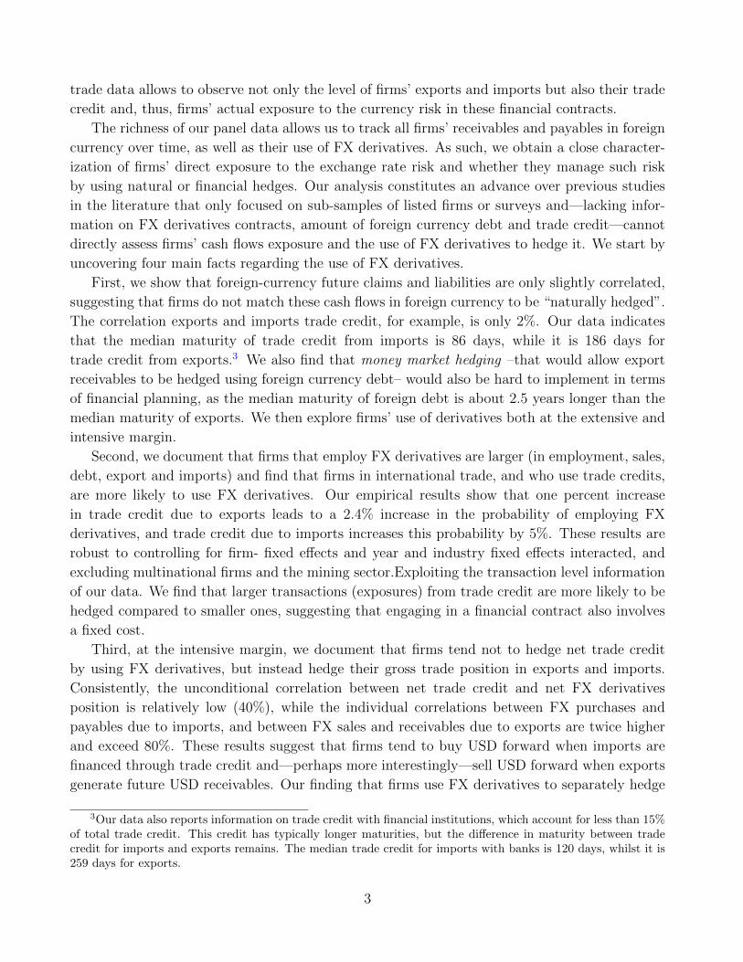
Gross FX-Derivatives position is the sum of long and short positions.Volume and number of firms consider only those in the non-financial corporate sector
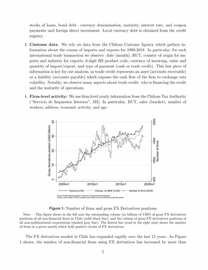
Figure 1: Number of firms and gross FX Derivatives positions
Note.— This figure shows in the left axis the outstanding volume (in billions of USD) of gross FX derivativespositions of all non-financial firms in Chile (solid black line), and the volume of gross FX derivatives positions ofall non-multinational corporations (dashed gray line). The dotted line (read in the right axis) shows the numberof firms in a given month which hold positive stocks of FX derivatives.
The FX derivatives market in Chile has expanded rapidly over the last 15 years. As Figure
1 shows, the number of non-financial firms using FX derivatives has increased by more than
7
two-fold, and their gross FX derivatives position has increased by four-fold, from 8 to more than
35 billion US dollars.9 Outstanding gross FX derivative positions reaches nowadays close to 45%
of GDP. In Panel A in Table 1 we report the market activity for the period 2005-2018 for the
whole market (columns 1-5), and for non-financial firms (columns 6-11). We have information
on roughly 1.9 million contracts, out of which 0.7 million contracts involve a non-financial firm
(columns 1 and 7). Forwards are firms’ most traded FX-derivative, representing nearly 90% of
all contracts. Their median maturity is 88 days, with longer maturities for sales than purchases
(Panel B). Also, around 80% (60%) of all sales (purchases) are settled with no delivery. The
second most used derivatives are swaps (both cross-currency and FX swaps), which account for
around 8% (5%) of purchases (sales) by non-financial firms. In the rest of the paper, we focus
our analysis on non-financial firms, which—for convenience—we thereafter simple name them as
firms.
To better identify firms’ currency exposure and hedging decisions, we focus on transactions
(trade, trade credit, foreign currency debt and FX derivatives) between U.S. dollars and Chilean
Pesos. This restriction is without loss of generality, as the U.S. dollar is the dominant foreign
currency in Chile and the majority of foreign currency transactions are with respect to this
currency (more 85%).10 We show in Appendix A.2 that our results hold true when we consider
all currencies in our analysis. The lion’s share of outstanding positions belongs to domestically-
owned firm (more than 90%). Importantly, the use of FX derivatives is spread across all economic
activities. The sectors using FX derivatives the most are retail trade, farming, electricity, water
supply and gas, non-metallic manufacturing, financial intermediation, mining and transport and
communication, which represent more than 90% of long and short FX positions in 2016. In
our main specification, we exclude MNCs, as these firms could use FX derivatives to hedge the
value of dividends in foreign currency, to hedge translation exposure, and their subsidiaries or
headquarters abroad may undertake the financial hedging. To check the validity of our results,
along the paper, we undertake several robustness with and without MNC. As mining sector
accounts for an important share of Chilean exports, we realize robustness with and without the
mining sector as well.
Beyond the granularity of the data, it is worth mentioning that Chile offers a good case to
study due to the stability of its macroeconomic and institutional framework. As detailed in the
next section, the derivatives market is dominated by over-the-counter transactions (OTC) as in
most developed economies; see, BIS(2016, 2019). Moreover, Chile has shown a combination of
responsible fiscal policy, freely floating exchange rate, and an inflation targeting regime imple-
9Our data contains financial and non-financial firms. Unless stated differently we will hereafter loosely referto non-financial firms when we use the term “firms”.
10In particular, in 2016, 94% of long FX positions and 87% of short FX positions had as counterpart the U.S.dollar. This was followed by the Euro with almost 5% and 6% long and short FX positions, respectively.
8
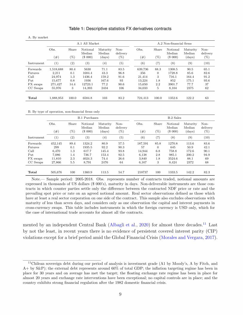
Table 1: Descriptive statistics FX derivatives contracts
A. By market
A.1 All Market A.2 Non-financial firms
Obs. Share NotionalMedian
MaturityMedian
Non-delivery
Obs. Share NotionalMedian
MaturityMedian
Non-delivery
(#) (%) ($ 000) (days) (%) (#) (%) ($ 000) (days) (%)
Instrument (1) (2) (3) (4) (5) (6) (7) (8) (9) (10)
Forwards 1,518,688 80.4 5630 71.1 83.5 639,736 88.3 1308.5 90.5 65.1Futures 2,211 0.1 1684.4 43.3 96.8 356 0 1728.8 85.6 82.6Call 24,974 1.3 1436.4 159.2 91.6 21,414 3 716.1 164.4 91.2Put 15,677 0.8 1936 167.6 93 13,224 1.8 852 175.1 93.6FX swaps 271,427 14.4 12723.1 77.2 90.6 15,650 2.2 3901.7 77.7 37CC Swaps 55,976 3 14,393 2434 106 34,033 5 8,104 2375 62
Total 1,888,953 100.0 6584.8 103 83.2 724,413 100.0 1352.6 122.2 63
B. By type of operation, non-financial firms only
B.1 Purchases B.2 Sales
Obs. Share NotionalMedian
MaturityMedian
Non-delivery
Obs. Share NotionalMedian
MaturityMedian
Non-delivery
(#) (%) ($ 000) (days) (%) (#) (%) ($ 000) (days) (%)
Instrument (1) (2) (3) (4) (5) (6) (7) (8) (9) (10)
Forwards 452,145 89.4 1324.2 80.9 57.5 187,591 85.8 1270.8 113.6 83.6Futures 299 0.1 1935.5 92.2 90.3 57 0 645 50.9 42.1Call 6,470 1.3 617.7 145.4 93.8 14,944 6.8 758.8 172.6 90.1Put 7,086 1.4 736.7 153.4 92.5 6,138 2.8 985.1 200.2 94.9FX swaps 11,810 2.3 4024.3 74.4 26.6 3,840 1.8 3524.6 88.1 69CC Swaps 27,866 5.5 8,791 2476 64 6,167 3 8,424 2372 68
Total 505,676 100 1360.9 113.5 54.7 218737 100 1333.5 142.2 82.3
Note.— Sample period: 2005-2018. Obs. represents number of contracts traded, notional amounts areexpressed in thousands of US dollars ($ 000’s), maturity in days. Non-deliverable instruments are those con-tracts in which counter parties settle only the difference between the contracted NDF price or rate and theprevailing spot price or rate on an agreed notional amount. Real sector observations defined as those whichhave at least a real sector corporation on one side of the contract. This sample also excludes observations withmaturity of less than seven days, and considers only as one observation the capital and interest payments incross-currency swaps. This table includes instruments in which the foreign currency is USD only, which forthe case of international trade accounts for almost all the contracts.
mented by an independent Central Bank (Albagli et al., 2020) for almost three decades.11 Last
by not the least, in recent years there is no evidence of persistent covered interest parity (CIP)
violations except for a brief period amid the Global Financial Crisis (Morales and Vergara, 2017).
11Chilean sovereign debt during our period of analysis is investment grade (A1 by Moody’s, A by Fitch, andA+ by S&P); the external debt represents around 60% of total GDP; the inflation targeting regime has been inplace for 30 years and on average has met the target; the floating exchange rate regime has been in place foralmost 20 years and exchange rate interventions have been exceptional; no capital controls are in place; and thecountry exhibits strong financial regulation after the 1982 domestic financial crisis.
9
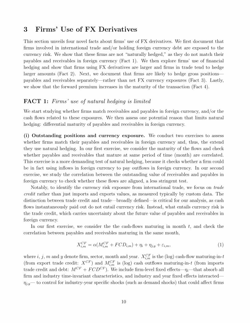
3 Firms’ Use of FX Derivatives
This section unveils four novel facts about firms’ use of FX derivatives. We first document that
firms involved in international trade and/or holding foreign currency debt are exposed to the
currency risk. We show that these firms are not “naturally hedged,” as they do not match their
payables and receivables in foreign currency (Fact 1). We then explore firms’ use of financial
hedging and show that firms using FX derivatives are larger and firms in trade tend to hedge
larger amounts (Fact 2). Next, we document that firms are likely to hedge gross positions—
payables and receivables separately—rather than net FX currency exposures (Fact 3). Lastly,
we show that the forward premium increases in the maturity of the transaction (Fact 4).
FACT 1: Firms’ use of natural hedging is limited
We start studying whether firms match receivables and payables in foreign currency, and/or the
cash flows related to these exposures. We then assess one potential reason that limits natural
hedging: differential maturity of payables and receivables in foreign currency.
(i) Outstanding positions and currency exposure. We conduct two exercises to assess
whether firms match their payables and receivables in foreign currency and, thus, the extend
they use natural hedging. In our first exercise, we consider the maturity of the flows and check
whether payables and receivables that mature at same period of time (month) are correlated.
This exercise is a more demanding test of natural hedging, because it checks whether a firm could
be in fact using inflows in foreign currency to pay outflows in foreign currency. In our second
exercise, we study the correlation between the outstanding value of receivables and payables in
foreign currency to check whether these flows are aligned, a less stringent test.
Notably, to identify the currency risk exposure from international trade, we focus on trade
credit rather than just imports and exports values, as measured typically by custom data. The
distinction between trade credit and trade—broadly defined—is critical for our analysis, as cash
flows instantaneously paid out do not entail currency risk. Instead, what entails currency risk is
the trade credit, which carries uncertainty about the future value of payables and receivables in
foreign currency.
In our first exercise, we consider the the cash-flows maturing in month t, and check the
correlation between payables and receivables maturing in the same month,
XCFi,m = α(MCF
i,m + FCDi,m) + ηi + ηj,y + εi,m, (1)
where i, j, m and y denote firm, sector, month and year. XCFi,m is the (log) cash-flow maturing-in-t
(from export trade credit: XCF ) and MCFi,m is (log) cash outflows maturing-in-t (from imports
trade credit and debt: MCF + FCDCF ). We include firm-level fixed effects—ηi—that absorb all
firm and industry time-invariant characteristics, and industry and year fixed effects interacted—
ηj,y— to control for industry-year specific shocks (such as demand shocks) that could affect firms
10
in different industries heterogeneously.12 We cluster the standard errors at the firm level. The
coefficient of interest is α, which captures the extend to which the value of cash-flow payables and
receivables in foreign currency are aligned. A value of α equal to one would imply full natural
hedge, as all cash-flow inflows and outflows in foreign currency would be highly correlated across
time. Instead, α equal to zero would imply no correlation between these flows and no room for
natural hedge.
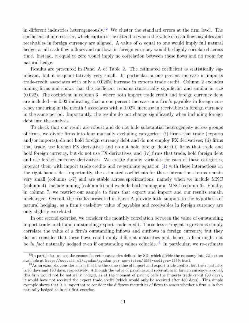
Results are presented in Panel A of Table 2. The estimated coefficient is statistically sig-
nificant, but it is quantitatively very small. In particular, a one percent increase in imports
trade-credit associates with only a 0.026% increase in exports trade credit. Column 2 excludes
mining firms and shows that the coefficient remains statistically significant and similar in size
(0.022). The coefficient in column 3—where both import trade credit and foreign currency debt
are included—is 0.02 indicating that a one percent increase in a firm’s payables in foreign cur-
rency maturing in the month t associates with a 0.02% increase in receivables in foreign currency
in the same period. Importantly, the results do not change significantly when including foreign
debt into the analysis.
To check that our result are robust and do not hide substantial heterogeneity across groups
of firms, we divide firms into four mutually excluding categories: (i) firms that trade (exports
and/or imports), do not hold foreign currency debt and do not employ FX derivatives; (ii) firms
that trade, use foreign FX derivatives and do not hold foreign debt; (iii) firms that trade and
hold foreign currency, but do not use FX derivatives; and (iv) firms that trade, hold foreign debt
and use foreign currency derivatives. We create dummy variables for each of these categories,
interact them with import trade credits and re-estimate equation (1) with these interactions on
the right hand side. Importantly, the estimated coefficients for these interactions terms remain
very small (columns 4-7) and are stable across specifications, namely when we include MNC
(column 4), include mining (column 5) and exclude both mining and MNC (column 6). Finally,
in column 7, we restrict our sample to firms that export and import and our results remain
unchanged. Overall, the results presented in Panel A provide little support to the hypothesis of
natural hedging, as a firm’s cash-flow value of payables and receivables in foreign currency are
only slightly correlated.
In our second exercise, we consider the monthly correlation between the value of outstanding
import trade credit and outstanding export trade credit. These less stringent regressions simply
correlate the value of a firm’s outstanding inflows and outflows in foreign currency, but they
do not consider that these flows could imply different maturities and, hence, a firm might not
be in fact naturally hedged even if outstanding values coincide.13 In particular, we re-estimate
12In particular, we use the economic sector categories defined by SII, which divide the economy into 22 sectorsavailable at http://www.sii.cl/ayudas/ayudas_por_servicios/1956-codigos-1959.html.
13As an example, consider a firm that has the same value of import and export trade credits, but their maturityis 30 days and 180 days, respectively. Although the value of payables and receivables in foreign currency is equal,this firm would not be naturally hedged, as at the moment of paying back the imports trade credit (30 days),it would have not received the export trade credit (which would only be received after 180 days). This simpleexample shows that it is important to consider the different maturities of flows to assess whether a firm is in factnaturally hedged as in our first exercise.
11
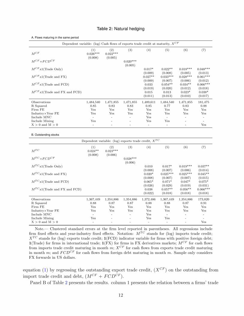
Table 2: Natural hedging
A. Flows maturing in the same period
Dependent variable: (log) Cash flows of exports trade credit at maturity, XCF
(1) (2) (3) (4) (5) (6) (7)MCF 0.026*** 0.022***
(0.008) (0.005)MCF +FCDCF 0.020***
(0.005)MCF x1(Trade Only) 0.017* 0.022** 0.018*** 0.048***
(0.009) (0.008) (0.005) (0.013)MCF x1(Trade and FX) 0.027** 0.033*** 0.028*** 0.061***
(0.009) (0.007) (0.006) (0.012)MCF x1(Trade and FCD) 0.033 0.054** 0.034** 0.066***
(0.019) (0.020) (0.012) (0.018)MCF x1(Trade and FX and FCD) 0.015 0.013 0.023* 0.038*
(0.011) (0.013) (0.010) (0.017)
Observations 1,484,540 1,471,855 1,471,855 1,489,611 1,484,540 1,471,855 181,475R Squared 0.85 0.83 0.83 0.85 0.77 0.83 0.88Firm FE Yes Yes Yes Yes Yes Yes YesIndustry×Year FE Yes Yes Yes Yes Yes Yes YesInclude MNC - - - Yes - - -Include Mining Yes - - Yes Yes - -X > 0 and M > 0 - - - - - - Yes
B. Outstanding stocks
Dependent variable: (log) exports trade credit, XTC
(1) (2) (3) (4) (5) (6) (7)MTC 0.024** 0.023***
(0.008) (0.006)MTC+FCDCF 0.028***
(0.006)MTCx1(Trade Only) 0.010 0.017* 0.019*** 0.037**
(0.008) (0.007) (0.006) (0.014)MTCx1(Trade and FX) 0.020* 0.025*** 0.025*** 0.045**
(0.008) (0.007) (0.007) (0.015)MTCx1(Trade and FCD) 0.065* 0.071* 0.047* 0.075*
(0.026) (0.029) (0.019) (0.031)MTCx1(Trade and FX and FCD) 0.038 0.057** 0.056** 0.066***
(0.022) (0.018) (0.018) (0.018)
Observations 1,367,449 1,354,886 1,354,886 1,372,486 1,367,449 1,354,886 173,820R Squared 0.88 0.87 0.87 0.88 0.88 0.87 0.91Firm FE Yes Yes Yes Yes Yes Yes YesIndustry×Year FE Yes Yes Yes Yes Yes Yes YesInclude MNC - - - Yes - - -Include Mining Yes - - Yes Yes - -X > 0 and M > 0 - - - - - - Yes
Note.— Clustered standard errors at the firm level reported in parentheses. All regressions includefirm fixed effects and year-industry fixed effects. Notation: MTC stands for (log) imports trade credit;XTC stands for (log) exports trade credit; 1(FCD) indicator variable for firms with positive foreign debt;1(Trade) for firms in international trade; 1(FX) for firms in FX derivatives markets; MCF for cash flowsfrom imports trade credit maturing in month m; XCF for cash flows from exports trade credit maturingin month m; and FCDCF for cash flows from foreign debt maturing in month m. Sample only considersFX forwards in US dollars.
equation (1) by regressing the outstanding export trade credit, (XCF ) on the outstanding from
import trade credit and debt, (MCF + FCDCF ).
Panel B of Table 2 presents the results. column 1 presents the relation between a firms’ trade
12
credit for export and imports. The estimated coefficients remain statistically significant, but as
above, they are quantitatively very small. In particular, a one percent increase in imports trade-
credit associates with only a 0.024% increase in exports trade credit in column 1 and . and similar
in size (0.023) when we exclude mining firm in Column 2. In column 3, we add foreign currency
debt to import trade credit and, thus, consider all foreign currency payables. Importantly, the
results do not change significantly when including foreign debt into the analysis. The estimated
coefficient remains quantitatively very small and indicates that a one percent increase the value of
foreign currency payables associates with only a 0.028% increase in the value of foreign currency
receivables. The estimated coefficients are similar in size across specifications.
In sum, the results presented in Table 2 provide little support to the hypothesis of natural
hedging. Firms in our sample do not seem to be using cash inflows and outflows in foreign
currency to operationally hedge the currency risk. Instead, these firms seems to be exposed to
the currency risk, which – in turn – create room to use financial hedging. We assess below a
potential reason that would explain this absence of natural hedging.
(ii) Maturity and the timing of flows. Last section showed that firms do not significantly
engage in natural hedging. In this section, we consider a potential explanation: different maturity
of inflows and outflows in foreign currency. In particular, if payables and receivables in foreign
currency have significantly different maturities, it could be difficult—from a management point
of view—to align these flows. It is worth noting that this section does not aim to provide one
conclusive explanation of why firms do not significantly engage in natural hedging. This would
require additional (and currently unavailable) information. Instead, we document some novel
patterns that could explain the limits to natural hedging reported above.
We start by documenting main descriptive statistics for imports/exports trade credit and
foreign borrowing. As Table 3 shows, trade credit from imports is paid on average in 91 days,
while exports take 137 days. Foreign debt exhibits even longer maturities, with an average of
3.7 years. The different maturity between trade credit from imports and exports and foreign
currency debt suggests that it would be difficult for firms to carry out operational hedging. This
type of hedging would imply significant managerial skills and planning to match the maturities
of multiple contracts.14
To explore further this idea, we focus on trade flows and examine the extent in which cash
flows of accounts payable/receivable coincide at maturity, regardless of contracting dates. More
precisely, consider equation (2) which captures the coincidence between cash inflows and outflows
from maturing trade-credit for each firm in a given month. In particular, for firm i and month
m, COi,m measures the coincident amount of cash flows (hence, the min operator) in opposing
directions that mature in m as a fraction of total cash flows maturing in the same period. The
statistic—multiplied by two to be bounded between 0 and 1—is defined by:
14Notably, these different maturities make it unlikely for firms to engage in “money market hedge”, whichrefers to an operation where a firm matches its receivables (payables) in foreign currency by borrowing (lending)in the same currency and maturity. For example, an exporter could borrow in foreign currency to hedge thecurrency risk implied in the future receivables. If the currency appreciates, she would receive lower income, butshe would also have a lower debt repayment in foreign currency.
13
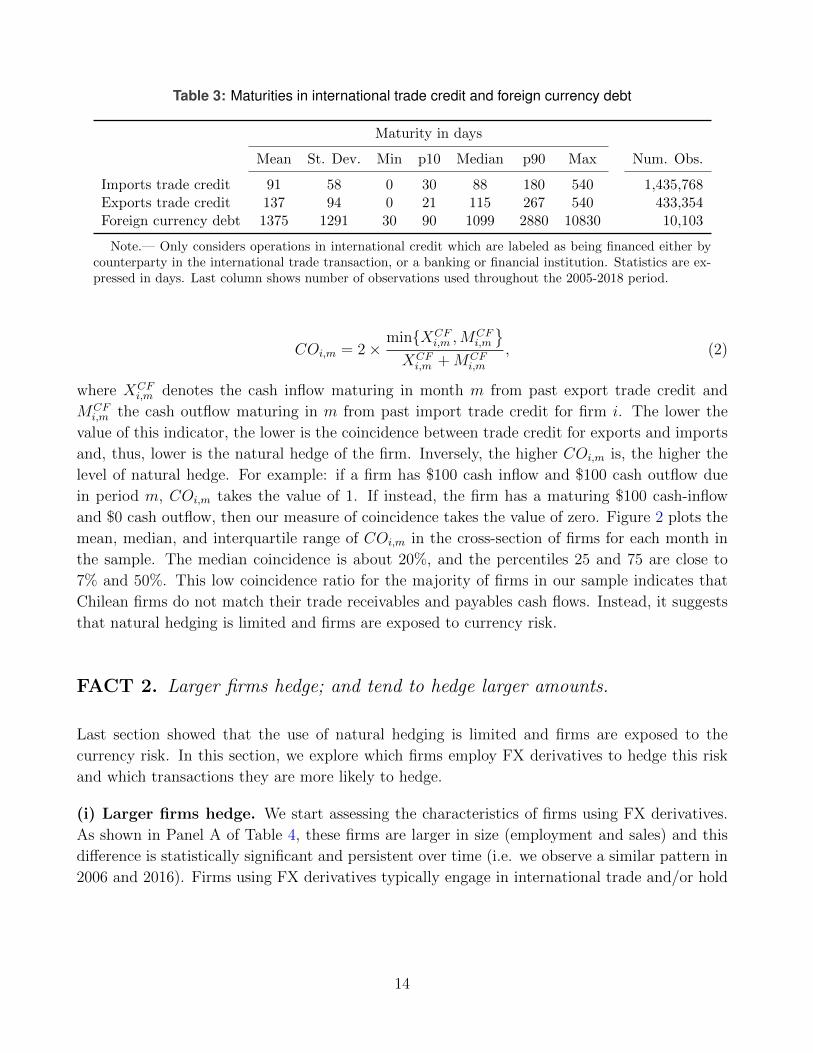
Table 3: Maturities in international trade credit and foreign currency debt
Maturity in days
Mean St. Dev. Min p10 Median p90 Max Num. Obs.
Imports trade credit 91 58 0 30 88 180 540 1,435,768Exports trade credit 137 94 0 21 115 267 540 433,354Foreign currency debt 1375 1291 30 90 1099 2880 10830 10,103
Note.— Only considers operations in international credit which are labeled as being financed either bycounterparty in the international trade transaction, or a banking or financial institution. Statistics are ex-pressed in days. Last column shows number of observations used throughout the 2005-2018 period.
COi,m = 2×min{XCF
i,m ,MCFi,m
}XCFi,m +MCF
i,m
, (2)
where XCFi,m denotes the cash inflow maturing in month m from past export trade credit and
MCFi,m the cash outflow maturing in m from past import trade credit for firm i. The lower the
value of this indicator, the lower is the coincidence between trade credit for exports and imports
and, thus, lower is the natural hedge of the firm. Inversely, the higher COi,m is, the higher the
level of natural hedge. For example: if a firm has $100 cash inflow and $100 cash outflow due
in period m, COi,m takes the value of 1. If instead, the firm has a maturing $100 cash-inflow
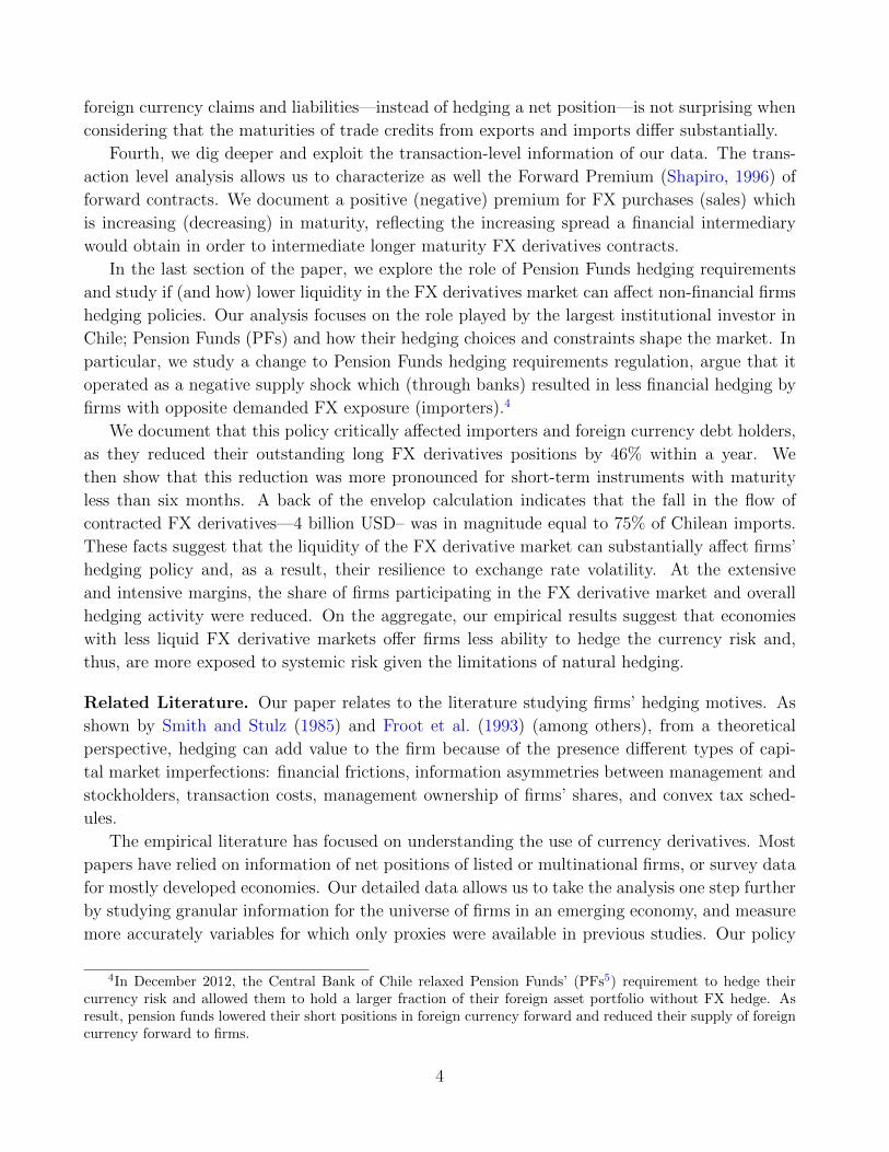
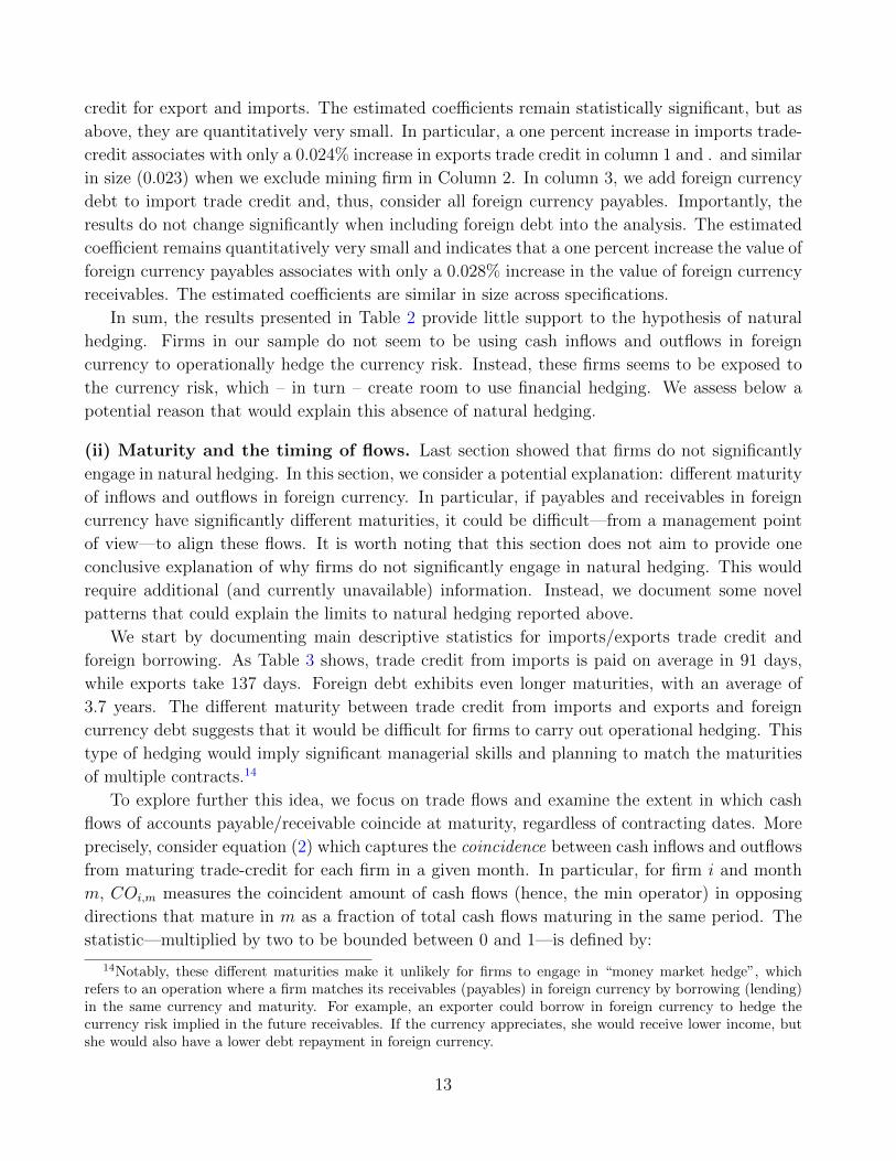
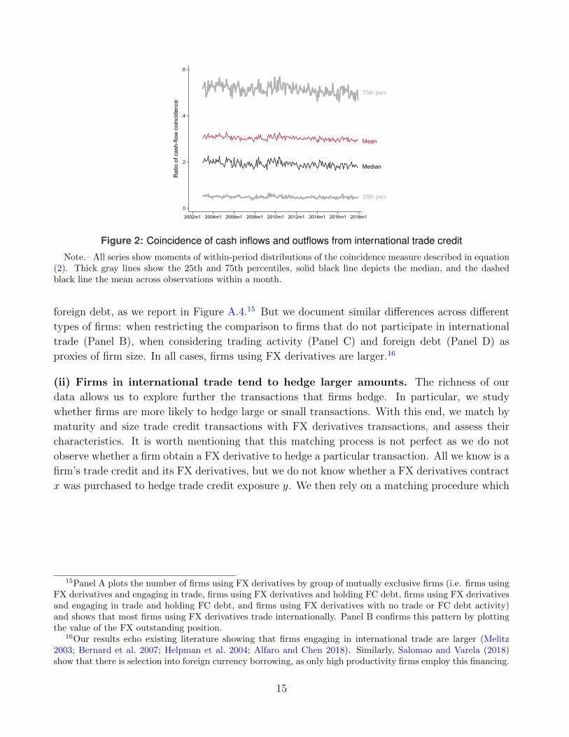
and $0 cash outflow, then our measure of coincidence takes the value of zero. Figure 2 plots the
mean, median, and interquartile range of COi,m in the cross-section of firms for each month in
the sample. The median coincidence is about 20%, and the percentiles 25 and 75 are close to
7% and 50%. This low coincidence ratio for the majority of firms in our sample indicates that
Chilean firms do not match their trade receivables and payables cash flows. Instead, it suggests
that natural hedging is limited and firms are exposed to currency risk.
FACT 2. Larger firms hedge; and tend to hedge larger amounts.
Last section showed that the use of natural hedging is limited and firms are exposed to the
currency risk. In this section, we explore which firms employ FX derivatives to hedge this risk
and which transactions they are more likely to hedge.
(i) Larger firms hedge. We start assessing the characteristics of firms using FX derivatives.
As shown in Panel A of Table 4, these firms are larger in size (employment and sales) and this
difference is statistically significant and persistent over time (i.e. we observe a similar pattern in
2006 and 2016). Firms using FX derivatives typically engage in international trade and/or hold
14
75th perc
25th perc
Median
Mean
0
.2
.4
.6
Rat
io o
f cas
h-flo
w c
oinc
iden
ce
2002m1 2004m1 2006m1 2008m1 2010m1 2012m1 2014m1 2016m1 2018m1
Figure 2: Coincidence of cash inflows and outflows from international trade credit
Note.– All series show moments of within-period distributions of the coincidence measure described in equation(2). Thick gray lines show the 25th and 75th percentiles, solid black line depicts the median, and the dashedblack line the mean across observations within a month.
foreign debt, as we report in Figure A.4.15 But we document similar differences across different
types of firms: when restricting the comparison to firms that do not participate in international
trade (Panel B), when considering trading activity (Panel C) and foreign debt (Panel D) as
proxies of firm size. In all cases, firms using FX derivatives are larger.16
(ii) Firms in international trade tend to hedge larger amounts. The richness of our
data allows us to explore further the transactions that firms hedge. In particular, we study
whether firms are more likely to hedge large or small transactions. With this end, we match by
maturity and size trade credit transactions with FX derivatives transactions, and assess their
characteristics. It is worth mentioning that this matching process is not perfect as we do not
observe whether a firm obtain a FX derivative to hedge a particular transaction. All we know is a
firm’s trade credit and its FX derivatives, but we do not know whether a FX derivatives contract
x was purchased to hedge trade credit exposure y. We then rely on a matching procedure which
15Panel A plots the number of firms using FX derivatives by group of mutually exclusive firms (i.e. firms usingFX derivatives and engaging in trade, firms using FX derivatives and holding FC debt, firms using FX derivativesand engaging in trade and holding FC debt, and firms using FX derivatives with no trade or FC debt activity)and shows that most firms using FX derivatives trade internationally. Panel B confirms this pattern by plottingthe value of the FX outstanding position.
16Our results echo existing literature showing that firms engaging in international trade are larger (Melitz2003; Bernard et al. 2007; Helpman et al. 2004; Alfaro and Chen 2018). Similarly, Salomao and Varela (2018)show that there is selection into foreign currency borrowing, as only high productivity firms employ this financing.
15
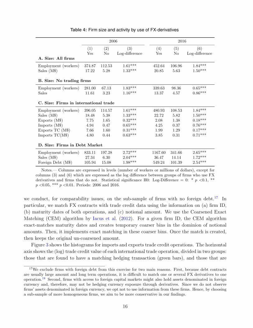
Table 4: Firm size and activity by use of FX-derivatives
2006 2016
(1) (2) (3) (4) (5) (6)Yes No Log-difference Yes No Log-difference
A. Size: All firms
Employment (workers) 374.87 112.53 1.61*** 452.64 106.96 1.84***Sales (M$) 17.22 5.28 1.33*** 20.85 5.63 1.50***
B. Size: No trading firms
Employment (workers) 281.00 67.13 1.83*** 339.63 98.36 0.65***Sales 11.61 3.23 1.16*** 13.37 4.57 0.86***
C. Size: Firms in international trade
Employment (workers) 396.05 114.57 1.61*** 480.93 108.53 1.84***Sales (M$) 18.48 5.38 1.33*** 22.72 5.82 1.50***Exports (M$) 7.75 1.65 0.32*** 2.08 1.38 0.18***Imports (M$) 4.94 0.47 0.65*** 4.25 0.37 0.76***Exports TC (M$) 7.66 1.60 0.31*** 1.99 1.29 0.17***Imports TC(M$) 4.80 0.44 0.63*** 3.85 0.31 0.71***
D. Size: Firms in Debt Market
Employment (workers) 833.11 197.28 2.72*** 1167.60 341.66 2.65***Sales (M$) 27.34 6.30 2.04*** 36.47 14.14 1.72***Foreign Debt (M$) 105.94 15.08 1.98*** 549.24 101.39 2.54***
Notes.— Columns are expressed in levels (number of workers or millions of dollars), except forcolumns (3) and (6) which are expressed as the log difference between groups of firms who use FXderivatives and firms that do not. Statistical significance H0: Log-Difference = 0: * p <0.1, **p <0.05, *** p <0.01. Periods: 2006 and 2016.
we conduct, for comparability issues, on the sub-sample of firms with no foreign debt.17 In
particular, we match FX contracts with trade credit data using the information on (a) firm ID,
(b) maturity dates of both operations, and (c) notional amount. We use the Coarsened Exact
Matching (CEM) algorithm by Iacus et al. (2012). For a given firm ID, the CEM algorithm
exact-matches maturity dates and creates temporary coarser bins in the dominion of notional
amounts. Then, it implements exact matching in these coarser bins. Once the match is created,
then keeps the original un-coarsened amount.
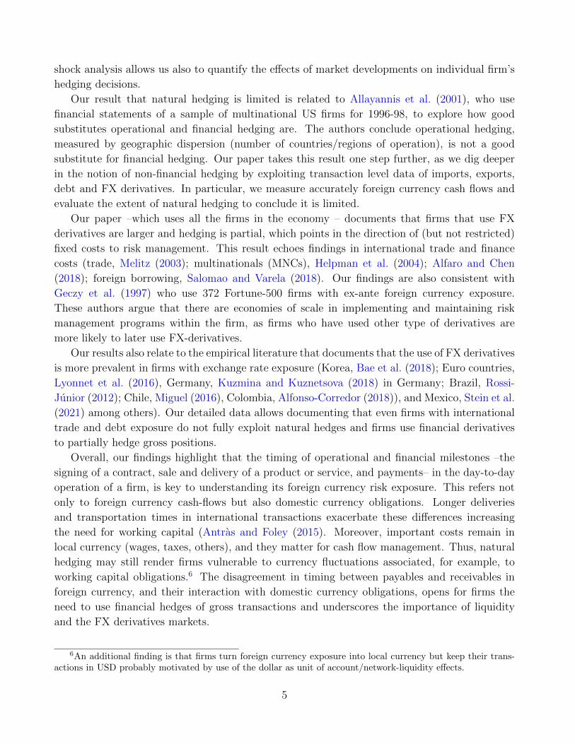
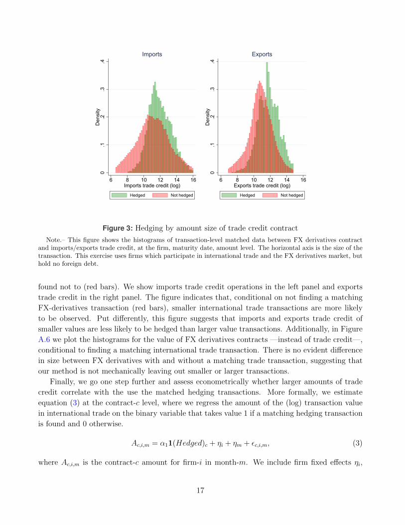
Figure 3 shows the histograms for imports and exports trade credit operations. The horizontal
axis shows the (log) trade credit value of each international trade operation, divided in two groups:
those that are found to have a matching hedging transaction (green bars), and those that are
17We exclude firms with foreign debt from this exercise for two main reasons. First, because debt contractsare usually large amount and long term operations, it is difficult to match one or several FX derivatives to oneoperation.18 Second, firms with access to foreign capital markets might also hold assets denominated in foreigncurrency and, therefore, may not be hedging currency exposure through derivatives. Since we do not observefirms’ assets denominated in foreign currency, we opt not to use information from these firms. Hence, by choosinga sub-sample of more homogeneous firms, we aim to be more conservative in our findings.
16
0.1
.2.3
.4D
ensi
ty
6 8 10 12 14 16Imports trade credit (log)
Hedged Not hedged
Imports
0.1
.2.3
.4D
ensi
ty
6 8 10 12 14 16Exports trade credit (log)
Hedged Not hedged
Exports
Figure 3: Hedging by amount size of trade credit contract
Note.– This figure shows the histograms of transaction-level matched data between FX derivatives contractand imports/exports trade credit, at the firm, maturity date, amount level. The horizontal axis is the size of thetransaction. This exercise uses firms which participate in international trade and the FX derivatives market, buthold no foreign debt.
found not to (red bars). We show imports trade credit operations in the left panel and exports
trade credit in the right panel. The figure indicates that, conditional on not finding a matching
FX-derivatives transaction (red bars), smaller international trade transactions are more likely
to be observed. Put differently, this figure suggests that imports and exports trade credit of
smaller values are less likely to be hedged than larger value transactions. Additionally, in Figure
A.6 we plot the histograms for the value of FX derivatives contracts —instead of trade credit—,
conditional to finding a matching international trade transaction. There is no evident difference
in size between FX derivatives with and without a matching trade transaction, suggesting that
our method is not mechanically leaving out smaller or larger transactions.
Finally, we go one step further and assess econometrically whether larger amounts of trade
credit correlate with the use the matched hedging transactions. More formally, we estimate
equation (3) at the contract-c level, where we regress the amount of the (log) transaction value
in international trade on the binary variable that takes value 1 if a matching hedging transaction
is found and 0 otherwise.
Ac,i,m = α11(Hedged)c + ηi + ηm + εc,i,m, (3)
where Ac,i,m is the contract-c amount for firm-i in month-m. We include firm fixed effects ηi,
17
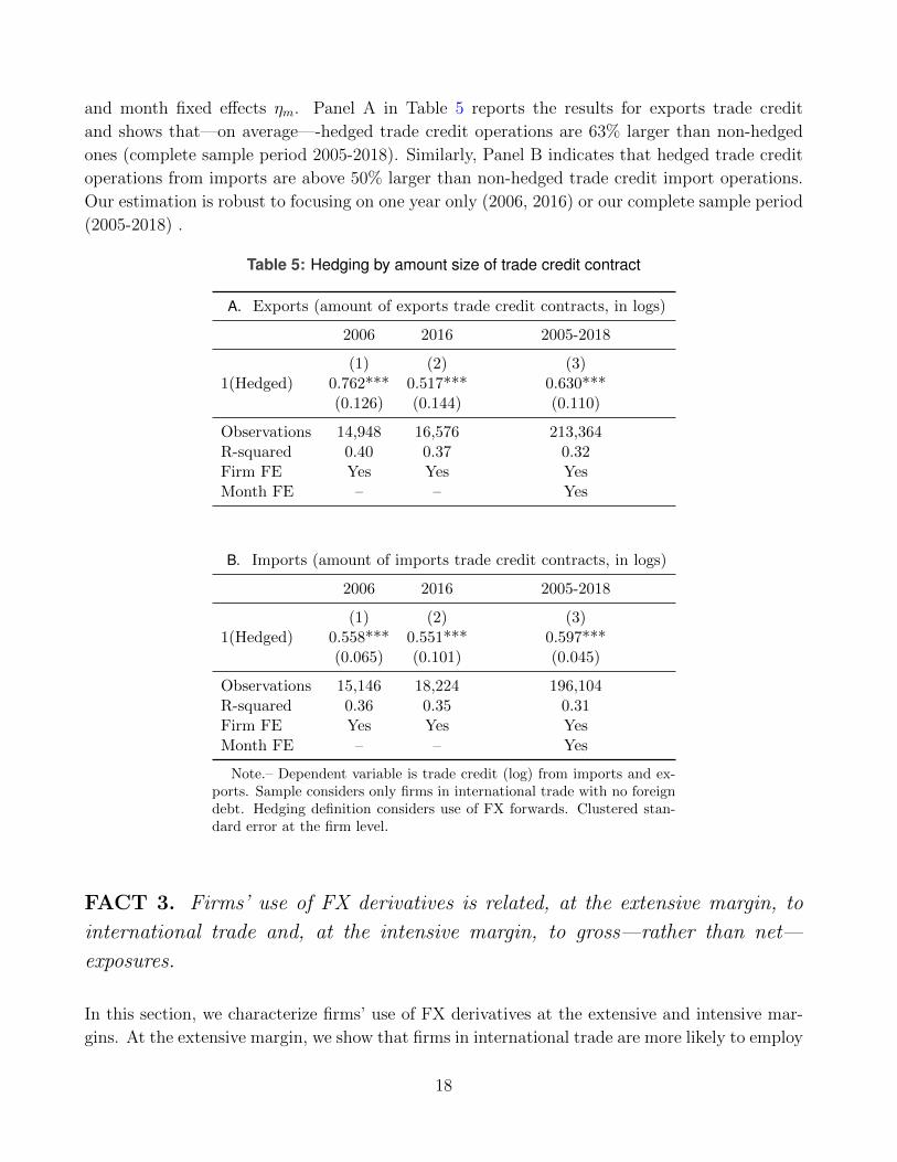
and month fixed effects ηm. Panel A in Table 5 reports the results for exports trade credit
and shows that—on average—-hedged trade credit operations are 63% larger than non-hedged
ones (complete sample period 2005-2018). Similarly, Panel B indicates that hedged trade credit
operations from imports are above 50% larger than non-hedged trade credit import operations.
Our estimation is robust to focusing on one year only (2006, 2016) or our complete sample period
(2005-2018) .
Table 5: Hedging by amount size of trade credit contract
A. Exports (amount of exports trade credit contracts, in logs)
2006 2016 2005-2018
(1) (2) (3)1(Hedged) 0.762*** 0.517*** 0.630***
(0.126) (0.144) (0.110)
Observations 14,948 16,576 213,364R-squared 0.40 0.37 0.32Firm FE Yes Yes YesMonth FE – – Yes
B. Imports (amount of imports trade credit contracts, in logs)
2006 2016 2005-2018
(1) (2) (3)1(Hedged) 0.558*** 0.551*** 0.597***
(0.065) (0.101) (0.045)
Observations 15,146 18,224 196,104R-squared 0.36 0.35 0.31Firm FE Yes Yes YesMonth FE – – Yes
Note.– Dependent variable is trade credit (log) from imports and ex-ports. Sample considers only firms in international trade with no foreigndebt. Hedging definition considers use of FX forwards. Clustered stan-dard error at the firm level.
FACT 3. Firms’ use of FX derivatives is related, at the extensive margin, to
international trade and, at the intensive margin, to gross—rather than net—
exposures.
In this section, we characterize firms’ use of FX derivatives at the extensive and intensive mar-
gins. At the extensive margin, we show that firms in international trade are more likely to employ
18
FX derivatives. At the intensive margin, we show that firms using FX derivatives hedge gross—
rather than net—currency risk exposures, which is consistent with the limited use of natural
hedging.
(i) The extensive margin. We start by studying the decision of a firm to use FX derivatives
by using nested versions of the following linear probability model:
FXi,m = β1XTCi,m + β2M
TCi,m + β3FCDi,m + ηi + ηj,y + εi,m, (4)
where FXi,m is a dummy equal to one if firm i has positive outstanding FX derivative position
at the end of the month m, and zero otherwise. XTCi,m , MTC
i,m and FCDi,m are (log) end-of-
month outstanding amounts of trade credit from exports and imports, and foreign currency
debt, respectively. We include firm and industry-year fixed effects, and cluster the standard
errors at the firm level.
Table 6: Use of FX derivatives: Extensive margin
Dependent variable 1(firm uses FX derivatives)
(1) (2) (3) (4) (5) (6) (7)XTC 0.020*** 0.019*** 0.022*** 0.022*** 0.018***
(0.005) (0.005) (0.005) (0.005) (0.004)MTC 0.049*** 0.048*** 0.053*** 0.052*** 0.057***
(0.005) (0.005) (0.006) (0.006) (0.005)FCD -0.014* -0.013* -0.011 -0.011 -0.006
(0.005) (0.006) (0.007) (0.006) (0.005)XTC ×MTC -0.009** -0.009* -0.007*
(0.003) (0.003) (0.003)XTC × FCD 0.002 0.002 -0.000
(0.003) (0.002) (0.002)MTC × FCD -0.006* -0.006* -0.006*
(0.003) (0.003) (0.003)
Observations 2,091,293 2,091,293 2,091,293 2,091,293 2,091,293 2,102,357 2,112,240R Squared 0.54 0.54 0.54 0.54 0.54 0.54 0.54Firm FE Yes Yes Yes Yes Yes Yes YesYear-Industry FE Yes Yes Yes Yes Yes Yes YesIncludes MNC - - - - - Yes YesIncludes Mining - - - - - - Yes
Notes.— All independent variables in logs. All regressions include firm level FE. XTC stands for exports tradecredit, MTC for imports trade credit, and FCD for the outstanding stock in foreign debt. Constant terms are notreported. Clustered standard errors at the firm level reported in parentheses. * p <0.1, ** p <0.05, *** p <0.01.
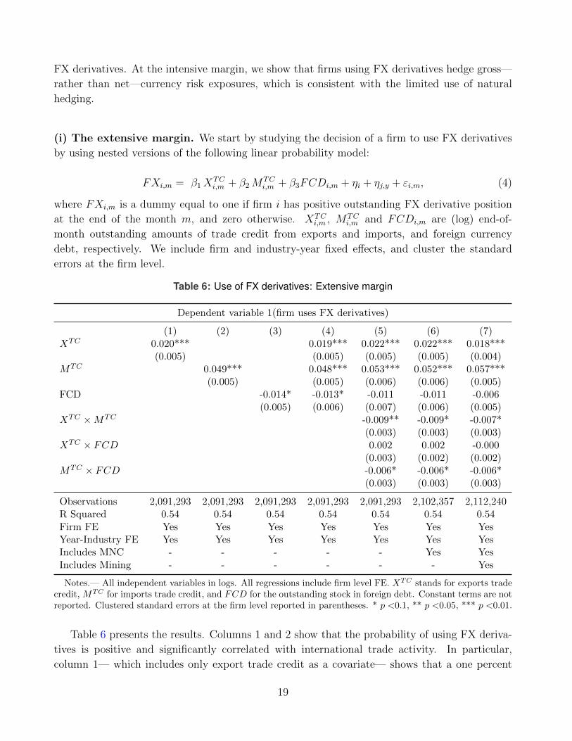
Table 6 presents the results. Columns 1 and 2 show that the probability of using FX deriva-
tives is positive and significantly correlated with international trade activity. In particular,
column 1— which includes only export trade credit as a covariate— shows that a one percent
19
increase in exports trade credit increases the probability of using FX derivatives 0.02 percentage
points. The probability of using FX derivatives is slightly higher for imports: 0.049 percent-
age points (column 2). Column 3 shows only a marginal correlation (and of the opposite sign)
between foreign debt and the probability of using FX derivatives.19 In column 4, we include
all three variables—export and import trade credits and foreign currency debt—and show that
the estimated coefficients for trade remain statistically significant and similar in size. Finally, in
columns 5 and 6, we control for exports, imports and foreign currency debt interacted, and show
that the estimated coefficients for trade credit remain similar to our previous estimates. In the
main specifications we exclude multinational and mining corporations, yet all results are robust
to this decision and across time sub-samples as seen in columns (6) and (7) (see Appendix for
additional robustness).
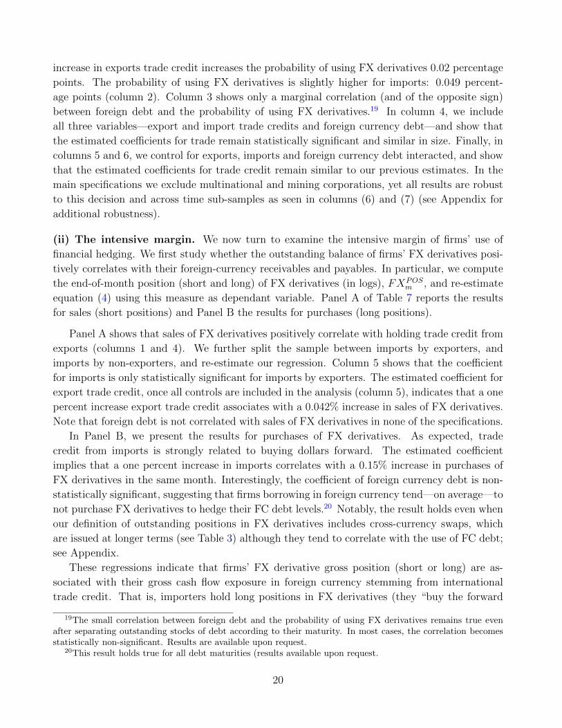
(ii) The intensive margin. We now turn to examine the intensive margin of firms’ use of
financial hedging. We first study whether the outstanding balance of firms’ FX derivatives posi-
tively correlates with their foreign-currency receivables and payables. In particular, we compute
the end-of-month position (short and long) of FX derivatives (in logs), FXPOSm , and re-estimate
equation (4) using this measure as dependant variable. Panel A of Table 7 reports the results
for sales (short positions) and Panel B the results for purchases (long positions).
Panel A shows that sales of FX derivatives positively correlate with holding trade credit from
exports (columns 1 and 4). We further split the sample between imports by exporters, and
imports by non-exporters, and re-estimate our regression. Column 5 shows that the coefficient
for imports is only statistically significant for imports by exporters. The estimated coefficient for
export trade credit, once all controls are included in the analysis (column 5), indicates that a one
percent increase export trade credit associates with a 0.042% increase in sales of FX derivatives.
Note that foreign debt is not correlated with sales of FX derivatives in none of the specifications.
In Panel B, we present the results for purchases of FX derivatives. As expected, trade
credit from imports is strongly related to buying dollars forward. The estimated coefficient
implies that a one percent increase in imports correlates with a 0.15% increase in purchases of
FX derivatives in the same month. Interestingly, the coefficient of foreign currency debt is non-
statistically significant, suggesting that firms borrowing in foreign currency tend—on average—to
not purchase FX derivatives to hedge their FC debt levels.20 Notably, the result holds even when
our definition of outstanding positions in FX derivatives includes cross-currency swaps, which
are issued at longer terms (see Table 3) although they tend to correlate with the use of FC debt;
see Appendix.
These regressions indicate that firms’ FX derivative gross position (short or long) are as-
sociated with their gross cash flow exposure in foreign currency stemming from international
trade credit. That is, importers hold long positions in FX derivatives (they “buy the forward
19The small correlation between foreign debt and the probability of using FX derivatives remains true evenafter separating outstanding stocks of debt according to their maturity. In most cases, the correlation becomesstatistically non-significant. Results are available upon request.
20This result holds true for all debt maturities (results available upon request.
20
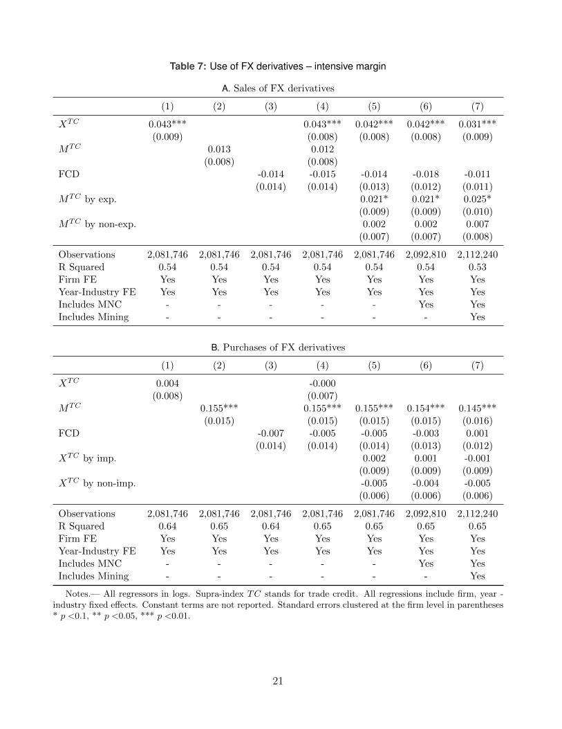
Table 7: Use of FX derivatives – intensive margin
A. Sales of FX derivatives
(1) (2) (3) (4) (5) (6) (7)
XTC 0.043*** 0.043*** 0.042*** 0.042*** 0.031***(0.009) (0.008) (0.008) (0.008) (0.009)
MTC 0.013 0.012(0.008) (0.008)
FCD -0.014 -0.015 -0.014 -0.018 -0.011(0.014) (0.014) (0.013) (0.012) (0.011)
MTC by exp. 0.021* 0.021* 0.025*(0.009) (0.009) (0.010)
MTC by non-exp. 0.002 0.002 0.007(0.007) (0.007) (0.008)
Observations 2,081,746 2,081,746 2,081,746 2,081,746 2,081,746 2,092,810 2,112,240R Squared 0.54 0.54 0.54 0.54 0.54 0.54 0.53Firm FE Yes Yes Yes Yes Yes Yes YesYear-Industry FE Yes Yes Yes Yes Yes Yes YesIncludes MNC - - - - - Yes YesIncludes Mining - - - - - - Yes
B. Purchases of FX derivatives
(1) (2) (3) (4) (5) (6) (7)
XTC 0.004 -0.000(0.008) (0.007)
MTC 0.155*** 0.155*** 0.155*** 0.154*** 0.145***(0.015) (0.015) (0.015) (0.015) (0.016)
FCD -0.007 -0.005 -0.005 -0.003 0.001(0.014) (0.014) (0.014) (0.013) (0.012)
XTC by imp. 0.002 0.001 -0.001(0.009) (0.009) (0.009)
XTC by non-imp. -0.005 -0.004 -0.005(0.006) (0.006) (0.006)
Observations 2,081,746 2,081,746 2,081,746 2,081,746 2,081,746 2,092,810 2,112,240R Squared 0.64 0.65 0.64 0.65 0.65 0.65 0.65Firm FE Yes Yes Yes Yes Yes Yes YesYear-Industry FE Yes Yes Yes Yes Yes Yes YesIncludes MNC - - - - - Yes YesIncludes Mining - - - - - - Yes
Notes.— All regressors in logs. Supra-index TC stands for trade credit. All regressions include firm, year -industry fixed effects. Constant terms are not reported. Standard errors clustered at the firm level in parentheses* p <0.1, ** p <0.05, *** p <0.01.
21
dollar”), while exporters hold short positions in FX derivatives (“they sell the forward dollar”).
The evidence presented in Tables 6, and 7 are robust to the inclusion/exclusion of multinational
corporations, firms related to the mining sector as seen in columns (6) and (7) and including
currencies different from the US dollar (see Appendix).
(iii) Aggregate trade credit and FX derivatives. The results in Table 7 suggest that the
gross amounts of imports and exports trade credit correlate with gross FX derivatives positions at
the firm level. We now assess whether this correlation of gross positions is present at the aggregate
level. With this end, we aggregate all export trade credit, all import trade credit and compare
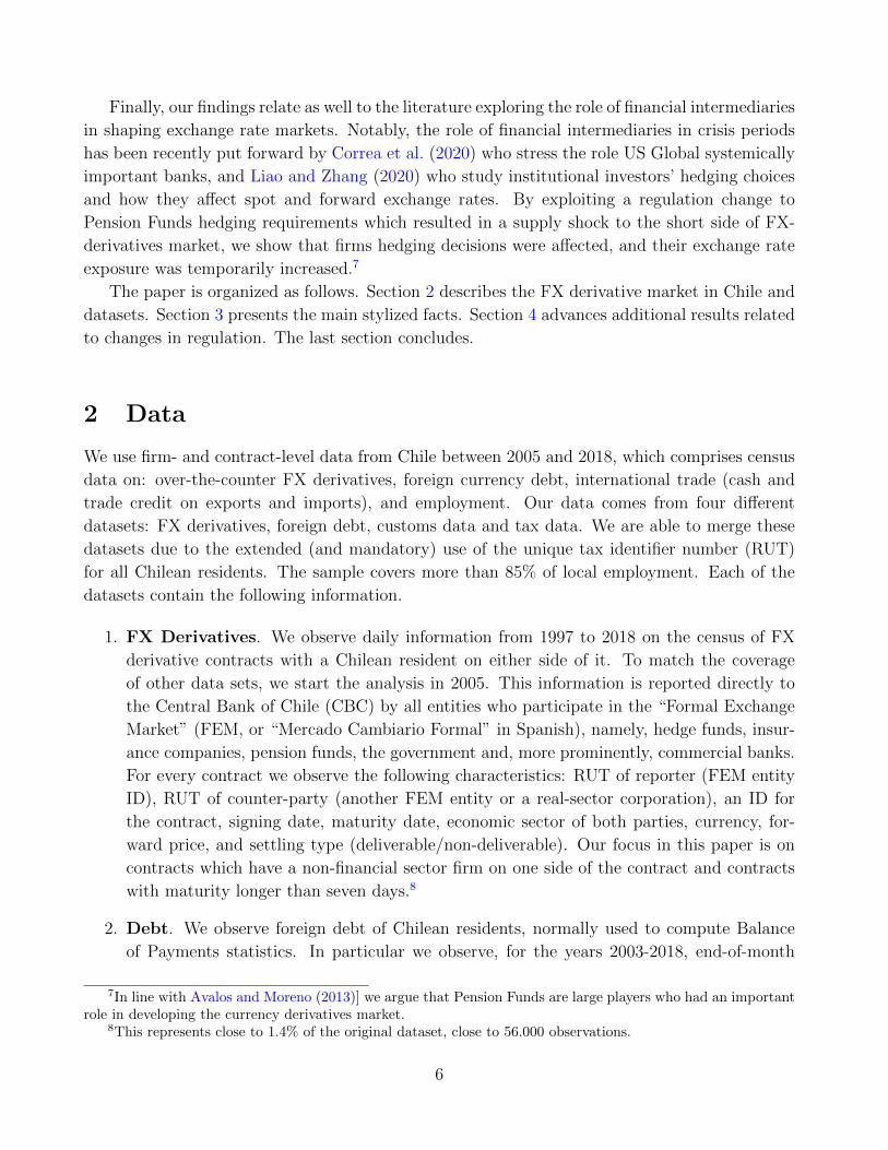
them with the FX derivatives sales and purchases. Figure 4 presents these correlations. The
correlation between exports trade credit and short FX positions—presented in Panel A— is high
and reaches 0.79. Similarly, the correlation between imports trade credit and long FX positions
– presented in Panel B – reaches 0.82. For comparison, in Panel C, we plot the correlation of net
trade credit with net FX derivatives position. Interesting, the correlation using net exposures is
much lower than the gross correlations and only reaches 0.48. Lastly, we conduct an additional
test and assess these correlations from an ex-post perspective. That is, we consider cash flows at
maturity date of FX contracts and obligations from derivatives positions, the same conclusion
holds. Notably, the correlation between imports trade credit maturing in month m and FX long
derivatives maturing in period m remains high at 0.9, and the correlation between exports trade
credit maturing in m and FX short derivatives maturing in the same period is close to 0.8.
A. Exports and FX sales
Exports
FX Sales
corr=0.790
1000
2000
3000
4000
5000
Milli
on U
SD
2005 2007 2009 2011 2013 2015 2017
B. Imports and FX purchases
Imports
FX Purchases
corr=0.820
1000
2000
3000
4000
5000
6000
Milli
on U
SD
2005 2007 2009 2011 2013 2015 2017
C. Net trade credit and NFXP
Net trade
Negative NDP
corr=0.48
-400
0-3
000
-200
0-1
000
010
00M
illion
USD
2005 2007 2009 2011 2013 2015 2017
Figure 4: Trade Credit balances related to international trade and FX gross derivatives positions
Note.– End-of-month balance from trade credit from exports and FX derivatives sales (Panel A.), importsand FX purchases (Panel B.), and net trade credit and (negative) net FX position (short minus long positions,Panel C.). Expressed in millions of dollars. Sample used in this figure excludes firms with foreign debt, to avoidbiasing upwards the estimation of the use of FX derivatives. Correlations between series are 0.79 for exports,and 0.82 for imports and 0.48 for net trade credit. Used sample also excludes multinational corporations, andmining companies. Inclusion of these firms does does not affect the results and can be seen in Figure A.5 in theAppendix.
22
FACT 4. FX derivatives contracts are priced differently according to maturity.
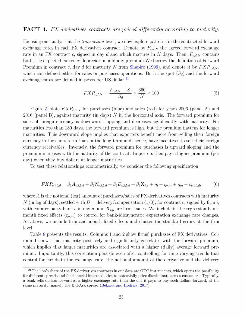
Focusing our analysis at the transaction level, we now explore patterns in the contracted forward
exchange rates in each FX derivatives contract. Denote by Fc,d,N the agreed forward exchange
rate in an FX contract c, signed in day d and which matures in N days. Then, Fc,d,N contains
both, the expected currency depreciation and any premium.We borrow the definition of Forward
Premium in contract c, day d for maturity N from Shapiro (1996), and denote it by FXPc,d,N ,
which can defined either for sales or purchases operations. Both the spot (Sd) and the forward
exchange rates are defined in pesos per US dollar.21
FXPc,d,N =Fc,d,N − Sd
Sd× 360
N× 100 (5)
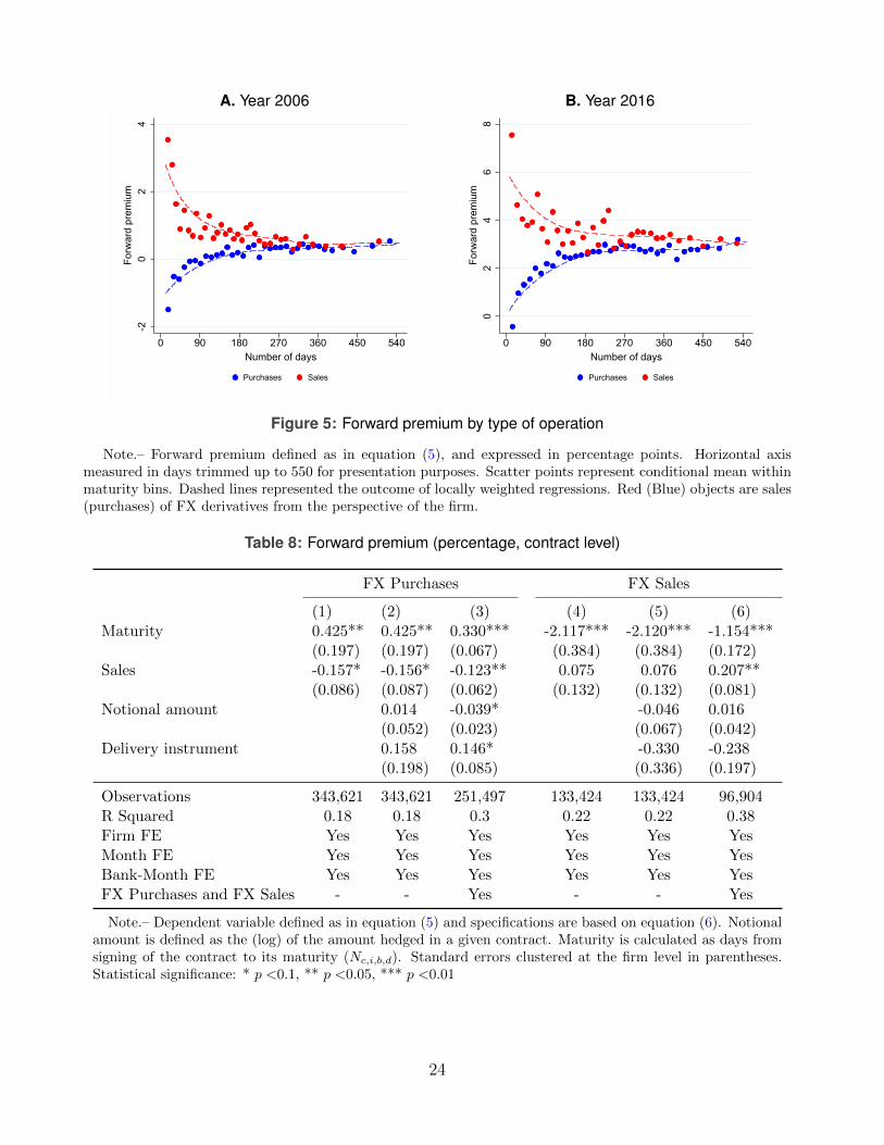
Figure 5 plots FXPc,d,N for purchases (blue) and sales (red) for years 2006 (panel A) and
2016 (panel B), against maturity (in days) N in the horizontal axis. The forward premium for
sales of foreign currency is downward slopping and decreases significantly with maturity. For
maturities less than 180 days, the forward premium is high, but the premium flattens for longer
maturities. This downward slope implies that exporters benefit more from selling their foreign
currency in the short term than in the long term and, hence, have incentives to sell their foreign
currency receivables. Inversely, the forward premium for purchases is upward sloping and the
premium increases with the maturity of the contract. Importers then pay a higher premium (per
day) when they buy dollars at longer maturities.
To test these relationships econometrically, we consider the following specification
FXPc,i,b,d = β1Ac,i,b,d + β2Nc,i,b,d + β3Dc,i,b,d + β4Xi,y + ηi + ηb,m + ηm + εc,i,b,d, (6)
where A is the notional (log) amount of purchases/sales of FX derivatives contracts with maturity
N (in log of days), settled with D = delivery/compensation (1/0), for contract c, signed by firm i,
with counter-party bank b in day d, and Xi,y are firms’ sales. We include in the regression bank-
month fixed effects (ηb,m) to control for bank-idiosyncratic expectation exchange rate changes.
As above, we include firm and month fixed effects and cluster the standard errors at the firm
level.
Table 8 presents the results. Columns 1 and 2 show firms’ purchases of FX derivatives. Col-
umn 1 shows that maturity positively and significantly correlates with the forward premium,
which implies that larger maturities are associated with a higher (daily) average forward pre-
mium. Importantly, this correlation persists even after controlling for time varying trends that
control for trends in the exchange rate, the notional amount of the derivative and the delivery
21The lion’s share of the FX derivatives contracts in our data are OTC instruments, which opens the possibilityfor different spreads and for financial intermediaries to potentially price discriminate across customers. Typically,a bank sells dollars forward at a higher exchange rate than the one it pays to buy such dollars forward, at thesame maturity; namely the Bid-Ask spread (Bekaert and Hodrick, 2017).
23
A. Year 2006
-20
24
Forw
ard
prem
ium
0 90 180 270 360 450 540Number of days
Purchases Sales
B. Year 2016
02
46
8Fo
rwar
d pr
emiu
m
0 90 180 270 360 450 540Number of days
Purchases Sales
Figure 5: Forward premium by type of operation
Note.– Forward premium defined as in equation (5), and expressed in percentage points. Horizontal axismeasured in days trimmed up to 550 for presentation purposes. Scatter points represent conditional mean withinmaturity bins. Dashed lines represented the outcome of locally weighted regressions. Red (Blue) objects are sales(purchases) of FX derivatives from the perspective of the firm.
Table 8: Forward premium (percentage, contract level)
FX Purchases FX Sales
(1) (2) (3) (4) (5) (6)Maturity 0.425** 0.425** 0.330*** -2.117*** -2.120*** -1.154***
(0.197) (0.197) (0.067) (0.384) (0.384) (0.172)Sales -0.157* -0.156* -0.123** 0.075 0.076 0.207**
(0.086) (0.087) (0.062) (0.132) (0.132) (0.081)Notional amount 0.014 -0.039* -0.046 0.016
(0.052) (0.023) (0.067) (0.042)Delivery instrument 0.158 0.146* -0.330 -0.238
(0.198) (0.085) (0.336) (0.197)
Observations 343,621 343,621 251,497 133,424 133,424 96,904R Squared 0.18 0.18 0.3 0.22 0.22 0.38Firm FE Yes Yes Yes Yes Yes YesMonth FE Yes Yes Yes Yes Yes YesBank-Month FE Yes Yes Yes Yes Yes YesFX Purchases and FX Sales - - Yes - - Yes
Note.– Dependent variable defined as in equation (5) and specifications are based on equation (6). Notionalamount is defined as the (log) of the amount hedged in a given contract. Maturity is calculated as days fromsigning of the contract to its maturity (Nc,i,b,d). Standard errors clustered at the firm level in parentheses.Statistical significance: * p <0.1, ** p <0.05, *** p <0.01
24
type instrument (column 2). Interesting, larger firms pay on average lower forward premium.
Columns 3 and 4 show that the forward premium negatively correlates with FX sales. That is,
when a firm wants to sell dollars forward, it gets a lower average daily premium the longer the
maturity of the instrument. These results suggest that the financial intermediary is charging a
higher bid-ask spread for transactions farther in the future, both for sales and purchases of FX
derivatives. Interestingly, the contract notional amount does not seem to have a robust influence
on the the forward premium charged neither for purchases nor for sales.
In the next section, we study whether the level of development and liquidity of the foreign
exchange rate market can affect firms’ hedging decisions. In particular, we exploit a regulatory
change to Pension Funds Managers (PFs)—which resulted in a temporary halt in their selling
of FX derivatives in 2012—to assess whether a negative supply shock affects firms’ hedging
choices. Finally, we revisit the potentially affected stylized facts in this section and document
their sensibility to the shock.
4 A Market-Level Supply Shock
In 2012, the Chilean Pensions Supervisor Authority (Superintendencia de Fondos de Pensiones)
relaxed the regulation on FX hedging by Pension Funds (PFs) with investments abroad. This
regulatory change had a large impact on the FX derivatives markets as PFs decreased their sales
of FX derivatives. These lower sales translated into a significant decrease in the supply of FX
derivatives from banks towards firms. In this section, we analyze how banks transmitted this
temporary liquidity shock and how it affected firms’ hedging patterns. We start by presenting
the regulatory change in the FX derivative markets and next describe the empirical strategy to
identify the impact of the shock on firms’ hedging decisions and prices in the forward market.
4.1 The Regulatory Change of the FX Derivative Markets
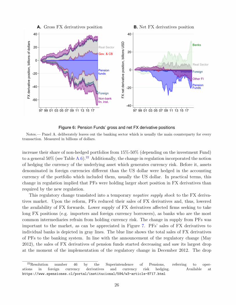
Pension funds are the backbone of the funded pension system in Chile. All non-military workers
save a mandatory 10% of their wages to finance their retirement income. They are the largest
holders of gross positions of FX derivatives. By the end of 2018, they held 41.3 billions of U.S
dollars in FX-derivatives, which is equivalent to 30% of the commercial banking credit and 15%
of GDP (Panel A. in Figure 6). Importantly, they are the agents with the largest net short FX
derivatives position and, at times, the only net suppliers of U.S. dollars in the forward market
(Panel B. in Figure 6). As such, they are the natural counter-party of the corporate sector, which
in net holds long positions. The supply of PFs’ net short position is intermediated to firms via
commercial banks through OTC FX derivatives.
Regulation dictates an upper limit, for each Fund, to the share of portfolio invested abroad
that is not hedged. In May 2012, the Pension Supervisor consulted the Central Bank of Chile
on their view of new limits for un-hedged portfolio invested abroad. After favorable assessment,
on June the regulator determined that starting on December 1st 2012, PFs would be allowed to
25
A. Gross FX derivatives position
Pensionfunds
Real Sector
Non-bankfin. inst.
Foreign
Gov. & CB
-60
-40
-20
0
20
40
FX d
eriv
ativ
e po
sitio
n, b
illion
s of
dol
lars
97 99 01 03 05 07 09 11 13 15 17
B. Net FX derivatives position
Real Sector
PensionFunds
Other FI
Foreign
Banks
-40
-20
0
20
40
FX n
et d
eriv
ativ
e po
sitio
n, b
illion
s U
SD
97 99 01 03 05 07 09 11 13 15 17
Figure 6: Pension Funds’ gross and net FX derivative positions
Notes.— Panel A. deliberately leaves out the banking sector which is usually the main counterparty for everytransaction. Measured in billions of dollars.
increase their share of non-hedged portfolios from 15%-50% (depending on the investment Fund)
to a general 50% (see Table A.6).22 Additionally, the change in regulation incorporated the notion
of hedging the currency of the underlying asset which generates currency risk. Before it, assets
denominated in foreign currencies different than the US dollar were hedged in the accounting
currency of the portfolio which included them, usually the US dollar. In practical terms, this
change in regulation implied that PFs were holding larger short position in FX derivatives than
required by the new regulation.
This regulatory change translated into a temporary negative supply shock to the FX deriva-
tives market. Upon the reform, PFs reduced their sales of FX derivatives and, thus, lowered
the availability of FX forwards. Lower supply of FX derivatives affected firms seeking to take
long FX positions (e.g. importers and foreign currency borrowers), as banks who are the most
common intermediaries refrain from holding currency risk. The change in supply from PFs was
important to the market, as can be appreciated in Figure 7. PFs’ sales of FX derivatives to
individual banks is depicted in gray lines. The blue line shows the total sales of FX derivatives
of PFs to the banking system. In line with the announcement of the regulatory change (May
2012), the sales of FX derivatives of pension funds started decreasing and saw its largest drop
at the moment of the implementation of the regulatory change in December 2012. The drop
22Resolution number 46 by the Superintendence of Pensions, referring to oper-ations in foreign currency derivatives and currency risk hedging. Available athttps://www.spensiones.cl/portal/institucional/594/w3-article-8717.html
26
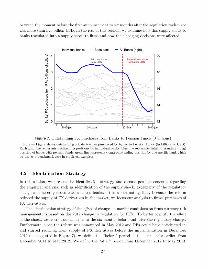
between the moment before the first announcement to six months after the regulation took place
was more than five billion USD. In the rest of this section, we examine how this supply shock to
banks translated into a supply shock to firms and how their hedging decisions were affected.
Regulation change(December 2012)
1st consultation(May 2012)
12
14
16
18
20
0
1
2
3
4
Bank
s' F
X pu
rcha
ses
from
PFs
(billi
ons
of d
olla
rs)
2012-jan 2012-jun 2013-jan 2013-jun
Individual banks Base bank All Banks (right)
Figure 7: Outstanding FX purchases from Banks to Pension Funds ($ billions)
Note.— Figure shows outstanding FX derivatives purchased by banks to Pension Funds (in billions of USD).Each gray line represents outstanding positions by individual banks; blue line represents total outstanding (long)position of banks with pension funds; green line represents (long) outstanding position by one specific bank whichwe use as a benchmark case in empirical exercises.
4.2 Identification Strategy
In this section, we present the identification strategy and discuss possible concerns regarding
the empirical analysis, such as identification of the supply shock, exogeneity of the regulatory
change and heterogeneous effects across banks. It is worth noting that, because the reform
reduced the supply of FX derivatives in the market, we focus our analysis to firms’ purchases of
FX derivatives.
The identification strategy of the effect of changes in market conditions on firms currency risk
management, is based on the 2012 change in regulation for PF’s. To better identify the effect
of the shock, we restrict our analysis to the six months before and after the regulatory change.
Furthermore, since the reform was announced in May 2012 and PFs could have anticipated it,
and started reducing their supply of FX derivatives before the implementation in December
2012 (as suggested in Figure 7), we define the “before” period as the six months earlier, from
December 2011 to May 2012. We define the “after” period from December 2012 to May 2013.
27
That is, we intentionally leave the months from June 2012 to November 2012 out of the analysis,
as these months could be considered partially treated due to the anticipation to the reform of
some PFs. This characterization has the additional advantage that it compares the same months
(December to May) and deals with seasonality that could arise from firms’ operating in different
economic activities. We refer to this analysis this analysis as the “six-month window”. To test
that our results are not driven by the length of the window, we conduct robustness tests with
“four-month window”, which cover December 2001- March 2012 and December 2012-March 2013
for the before and after periods.
An important concern of the empirical analysis is that a decrease in firms’ demand for FX
derivatives, rather than a negative supply shock, could arise from changes in firms’ hedging
policies. Because in Chile FX derivatives are mostly transacted through OTC market with
the banking sector, we can follow Khwaja and Mian (2008), Amiti and Weinstein (2018) and
Alfaro et al. (2020) and exploit firms’ multi-bank relationship to control for firms’ demand
of Fx derivatives.23 In particular, we keep firms that have hedging activities with more than
two banks and include in our regressions firm-time fixed effects. This allows us to control for
firms’ time-varying demand of hedging instruments and capture only the supply shock due to
the regulatory change on pension funds. Furthermore, this identification strategy allows us to
recover the decrease in the supply of FX derivatives of each individual bank and, hence, observe
the heterogeneous impact of the regulatory shock across banks. As additional test, we check
(and confirm) that the estimated coefficients for banks correlate with their pre-reform exposure
to pension funds. More precisely, we show that banks that purchased more FX derivatives from
pension funds before the shock—and, hence, were more exposed to the regulatory change—
experienced a larger decrease in the sales of FX derivatives to firms after the implementation of
the regulation.
The analyzed change in regulation was arguably exogenous to firms’ individual hedging de-
cisions. The general context around the regulatory change, and its timing make it unlikely that
firms hedging decisions were endogenous to the policy change by the Pension Funds Supervisor.
Furthermore, as mentioned above, we focus our analysis in the period before the announcement
of the policy, so we can avoid any anticipation effect from firms and, hence, simultaneity bias.
4.3 Empirical Results
In this section, we study whether the decrease in the supply of FX derivatives issued by PFs
affected firms’ hedging activity by conducting four econometric exercises. First, we estimate a
standard difference-in-difference model where we estimate the average response of firms across
all banks. Second, we saturate our regressions with time-varying firm and bank fixed effects
to control for changes in firms’ hedging demand and capture banks’ individual changes in the
23In Khwaja and Mian (2008), Amiti and Weinstein (2018) and Alfaro et al. (2020) the identification relies indisentangling the bank lending channel (the bank-specific shock) from the firm borrowing channel (the ability offirms to borrow from alternative sources). Our question is similar, but is not concerned with loans contracts butwith hedging.
28
supply of FX derivatives to firms. Additionally, we assess whether these changes associate with
changes in the forward premium and, hence, the price of FX derivatives. Third, we conduct a
back-of-the-envelope calculation to assess the aggregate impact of the regulatory change on firms’
hedging policies. Four, we study whether the supply shock affected firms’ hedging decisions at
the intensive and extensive margins.
4.3.1 Average Effect Across Banks
We start our analysis with a standard difference-in-difference estimator, in which we estimate the
average impact of the regulatory change on firms’ hedging positions across banks. With this end,
we define a dummy variable Postτ which takes the value of zero before the regulatory change,
and one after it. More precisely, we estimate:
FXLongi,τ = β1 Postτ + ηi + εi,τ , (7)
where τ denotes the period before and after the reform, FXLongi,τ is the (log) average outstanding
long derivatives position of firm i in period τ (before or after the shock), and ηi are firm fixed
effects.
Table 9 presents the results of estimating equation (7) with our benchmark before/after time
windows of 6 months in Panel A and shorter time windows of four months in Panel B. Columns
1 to 3 in both panels use as the dependent variable the (log) average outstanding long FX
derivatives position. Columns 4 to 6, instead, use as dependent variable the annual growth rate
of said variable. We include firm FE across all specifications, include industry FE in columns 2,
3, 5 and 6, and exclude mining and multinational corporations in columns 3 and 6. Results are
robust to these choices. In particular, we see that after the change in regulation, firms contracted
their purchases by around 8% and reduced their growth rate in half.
4.3.2 Banks’ Individual Supply Changes of FX Derivatives
The above analysis does not control for changes in firms’ hedging demand over time and, hence, it
could be attributing changes in demand to the regulatory change on the pension funds. To assess
whether the estimated coefficients correspond to the supply shock and not a lower demand of
FX derivatives from firms, we conduct an additional exercise where we saturate our regressions
with time-varying firm fixed effects and banks fixed effects. We exploit firms’ multi-banking
relationships to identify the supply shocks. This identification strategy allows us to obtain
banks’ individual coefficients that capture the change in the supply of FX derivatives to firms,
once firms’ demand for FX derivatives is already controlled for. In particular, we consider the
following specification,
D(FXi,b,τ ) = αi,τ + βb,τ + εi,b,τ , (8)
29
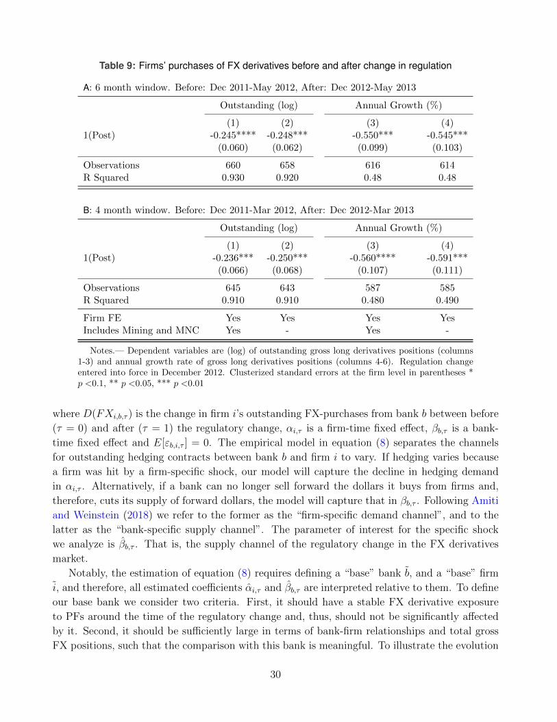
Table 9: Firms’ purchases of FX derivatives before and after change in regulation
A: 6 month window. Before: Dec 2011-May 2012, After: Dec 2012-May 2013
Outstanding (log) Annual Growth (%)
(1) (2) (3) (4)1(Post) -0.245**** -0.248*** -0.550*** -0.545***
(0.060) (0.062) (0.099) (0.103)
Observations 660 658 616 614R Squared 0.930 0.920 0.48 0.48
B: 4 month window. Before: Dec 2011-Mar 2012, After: Dec 2012-Mar 2013
Outstanding (log) Annual Growth (%)
(1) (2) (3) (4)1(Post) -0.236*** -0.250*** -0.560**** -0.591***
(0.066) (0.068) (0.107) (0.111)
Observations 645 643 587 585R Squared 0.910 0.910 0.480 0.490
Firm FE Yes Yes Yes YesIncludes Mining and MNC Yes - Yes -
Notes.— Dependent variables are (log) of outstanding gross long derivatives positions (columns1-3) and annual growth rate of gross long derivatives positions (columns 4-6). Regulation changeentered into force in December 2012. Clusterized standard errors at the firm level in parentheses *p <0.1, ** p <0.05, *** p <0.01
where D(FXi,b,τ ) is the change in firm i’s outstanding FX-purchases from bank b between before
(τ = 0) and after (τ = 1) the regulatory change, αi,τ is a firm-time fixed effect, βb,τ is a bank-
time fixed effect and E[εb,i,τ ] = 0. The empirical model in equation (8) separates the channels
for outstanding hedging contracts between bank b and firm i to vary. If hedging varies because
a firm was hit by a firm-specific shock, our model will capture the decline in hedging demand
in αi,τ . Alternatively, if a bank can no longer sell forward the dollars it buys from firms and,
therefore, cuts its supply of forward dollars, the model will capture that in βb,τ . Following Amiti
and Weinstein (2018) we refer to the former as the “firm-specific demand channel”, and to the
latter as the “bank-specific supply channel”. The parameter of interest for the specific shock
we analyze is βb,τ . That is, the supply channel of the regulatory change in the FX derivatives
market.
Notably, the estimation of equation (8) requires defining a “base” bank b, and a “base” firm
i, and therefore, all estimated coefficients αi,τ and βb,τ are interpreted relative to them. To define
our base bank we consider two criteria. First, it should have a stable FX derivative exposure
to PFs around the time of the regulatory change and, thus, should not be significantly affected
by it. Second, it should be sufficiently large in terms of bank-firm relationships and total gross
FX positions, such that the comparison with this bank is meaningful. To illustrate the evolution
30
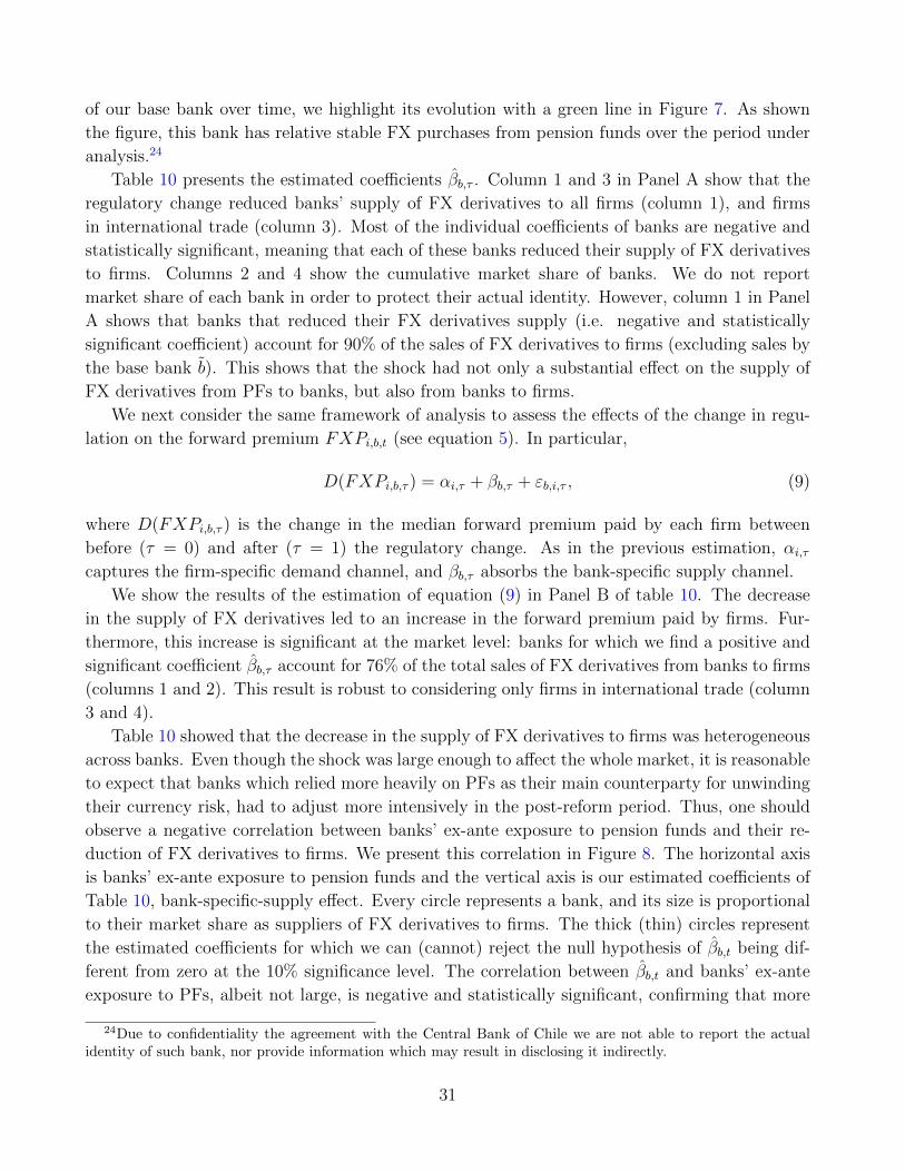
of our base bank over time, we highlight its evolution with a green line in Figure 7. As shown
the figure, this bank has relative stable FX purchases from pension funds over the period under
analysis.24
Table 10 presents the estimated coefficients βb,τ . Column 1 and 3 in Panel A show that the
regulatory change reduced banks’ supply of FX derivatives to all firms (column 1), and firms
in international trade (column 3). Most of the individual coefficients of banks are negative and
statistically significant, meaning that each of these banks reduced their supply of FX derivatives
to firms. Columns 2 and 4 show the cumulative market share of banks. We do not report
market share of each bank in order to protect their actual identity. However, column 1 in Panel
A shows that banks that reduced their FX derivatives supply (i.e. negative and statistically
significant coefficient) account for 90% of the sales of FX derivatives to firms (excluding sales by
the base bank b). This shows that the shock had not only a substantial effect on the supply of
FX derivatives from PFs to banks, but also from banks to firms.
We next consider the same framework of analysis to assess the effects of the change in regu-
lation on the forward premium FXPi,b,t (see equation 5). In particular,
D(FXPi,b,τ ) = αi,τ + βb,τ + εb,i,τ , (9)
where D(FXPi,b,τ ) is the change in the median forward premium paid by each firm between
before (τ = 0) and after (τ = 1) the regulatory change. As in the previous estimation, αi,τcaptures the firm-specific demand channel, and βb,τ absorbs the bank-specific supply channel.
We show the results of the estimation of equation (9) in Panel B of table 10. The decrease
in the supply of FX derivatives led to an increase in the forward premium paid by firms. Fur-
thermore, this increase is significant at the market level: banks for which we find a positive and
significant coefficient βb,τ account for 76% of the total sales of FX derivatives from banks to firms
(columns 1 and 2). This result is robust to considering only firms in international trade (column
3 and 4).
Table 10 showed that the decrease in the supply of FX derivatives to firms was heterogeneous
across banks. Even though the shock was large enough to affect the whole market, it is reasonable
to expect that banks which relied more heavily on PFs as their main counterparty for unwinding
their currency risk, had to adjust more intensively in the post-reform period. Thus, one should
observe a negative correlation between banks’ ex-ante exposure to pension funds and their re-
duction of FX derivatives to firms. We present this correlation in Figure 8. The horizontal axis
is banks’ ex-ante exposure to pension funds and the vertical axis is our estimated coefficients of
Table 10, bank-specific-supply effect. Every circle represents a bank, and its size is proportional
to their market share as suppliers of FX derivatives to firms. The thick (thin) circles represent
the estimated coefficients for which we can (cannot) reject the null hypothesis of βb,t being dif-
ferent from zero at the 10% significance level. The correlation between βb,t and banks’ ex-ante
exposure to PFs, albeit not large, is negative and statistically significant, confirming that more
24Due to confidentiality the agreement with the Central Bank of Chile we are not able to report the actualidentity of such bank, nor provide information which may result in disclosing it indirectly.
31
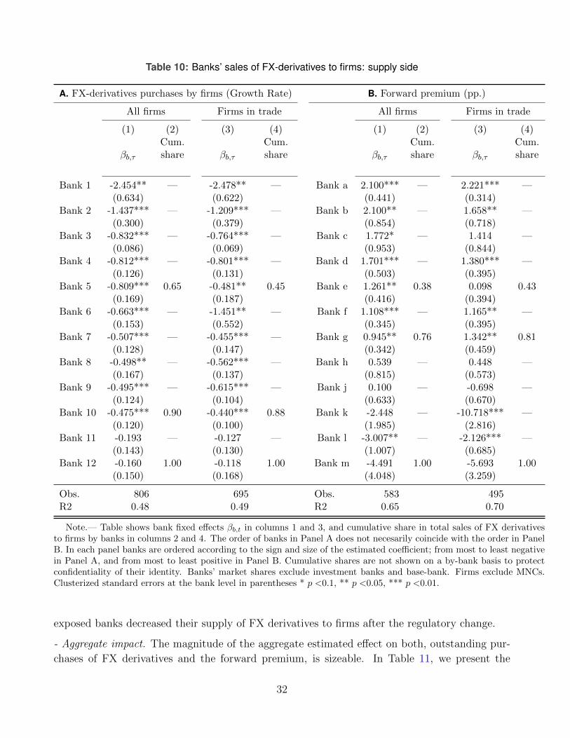
Table 10: Banks’ sales of FX-derivatives to firms: supply side
A. FX-derivatives purchases by firms (Growth Rate) B. Forward premium (pp.)
All firms Firms in trade All firms Firms in trade
(1) (2) (3) (4) (1) (2) (3) (4)Cum. Cum. Cum. Cum.
βb,τ share βb,τ share βb,τ share βb,τ share
Bank 1 -2.454** — -2.478** — Bank a 2.100*** — 2.221*** —(0.634) (0.622) (0.441) (0.314)
Bank 2 -1.437*** — -1.209*** — Bank b 2.100** — 1.658** —(0.300) (0.379) (0.854) (0.718)
Bank 3 -0.832*** — -0.764*** — Bank c 1.772* — 1.414 —(0.086) (0.069) (0.953) (0.844)
Bank 4 -0.812*** — -0.801*** — Bank d 1.701*** — 1.380*** —(0.126) (0.131) (0.503) (0.395)
Bank 5 -0.809*** 0.65 -0.481** 0.45 Bank e 1.261** 0.38 0.098 0.43(0.169) (0.187) (0.416) (0.394)
Bank 6 -0.663*** — -1.451** — Bank f 1.108*** — 1.165** —(0.153) (0.552) (0.345) (0.395)
Bank 7 -0.507*** — -0.455*** — Bank g 0.945** 0.76 1.342** 0.81(0.128) (0.147) (0.342) (0.459)
Bank 8 -0.498** — -0.562*** — Bank h 0.539 — 0.448 —(0.167) (0.137) (0.815) (0.573)
Bank 9 -0.495*** — -0.615*** — Bank j 0.100 — -0.698 —(0.124) (0.104) (0.633) (0.670)
Bank 10 -0.475*** 0.90 -0.440*** 0.88 Bank k -2.448 — -10.718*** —(0.120) (0.100) (1.985) (2.816)
Bank 11 -0.193 — -0.127 — Bank l -3.007** — -2.126*** —(0.143) (0.130) (1.007) (0.685)
Bank 12 -0.160 1.00 -0.118 1.00 Bank m -4.491 1.00 -5.693 1.00(0.150) (0.168) (4.048) (3.259)
Obs. 806 695 Obs. 583 495R2 0.48 0.49 R2 0.65 0.70
Note.— Table shows bank fixed effects βb,t in columns 1 and 3, and cumulative share in total sales of FX derivativesto firms by banks in columns 2 and 4. The order of banks in Panel A does not necesarily coincide with the order in PanelB. In each panel banks are ordered according to the sign and size of the estimated coefficient; from most to least negativein Panel A, and from most to least positive in Panel B. Cumulative shares are not shown on a by-bank basis to protectconfidentiality of their identity. Banks’ market shares exclude investment banks and base-bank. Firms exclude MNCs.Clusterized standard errors at the bank level in parentheses * p <0.1, ** p <0.05, *** p <0.01.
exposed banks decreased their supply of FX derivatives to firms after the regulatory change.
- Aggregate impact. The magnitude of the aggregate estimated effect on both, outstanding pur-
chases of FX derivatives and the forward premium, is sizeable. In Table 11, we present the
32
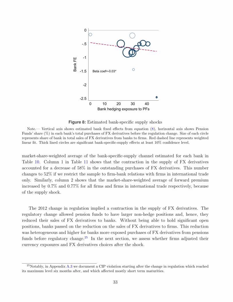
Beta coef=-0.03*
-2.5
-2
-1.5
-1
-.5
0
Bank
FE
0 10 20 30 40Bank hedging exposure to PFs
Figure 8: Estimated bank-specific supply shocks
Note.— Vertical axis shows estimated bank fixed effects from equation (8), horizontal axis shows PensionFunds’ share (%) in each bank’s total purchases of FX derivatives before the regulation change. Size of each circlerepresents share of bank in total sales of FX derivatives from banks to firms. Red dashed line represents weightedlinear fit. Thick lined circles are significant bank-specific-supply effects at least 10% confidence level.
market-share-weighted average of the bank-specific-supply channel estimated for each bank in
Table 10. Column 1 in Table 11 shows that the contraction in the supply of FX derivatives
accounted for a decrease of 58% in the outstanding purchases of FX derivatives. This number
changes to 52% if we restrict the sample to firm-bank relations with firms in international trade
only. Similarly, column 2 shows that the market-share-weighted average of forward premium
increased by 0.7% and 0.77% for all firms and firms in international trade respectively, because
of the supply shock.
The 2012 change in regulation implied a contraction in the supply of FX derivatives. The
regulatory change allowed pension funds to have larger non-hedge positions and, hence, they
reduced their sales of FX derivatives to banks. Without being able to hold significant open
positions, banks passed on the reduction on the sales of FX derivatives to firms. This reduction
was heterogeneous and higher for banks more exposed purchases of FX derivatives from pensions
funds before regulatory change.25 In the next section, we assess whether firms adjusted their
currency exposures and FX derivatives choices after the shock.
25Notably, in Appendix A.3 we document a CIP violation starting after the change in regulation which reachedits maximum level six months after, and which affected mostly short term maturities.
33
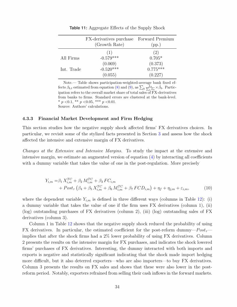
Table 11: Aggregate Effects of the Supply Shock
FX-derivatives purchase Forward Premium(Growth Rate) (pp.)
(1) (2)All Firms -0.579*** 0.705*
(0.069) (0.373)Int. Trade -0.520*** 0.775***
(0.055) (0.227)
Note.— Table shows participation-weighted-average bank fixed ef-fects βb,t estimated from equation (8) and (9), as
∑b
Lb∑b Lb×βb. Partic-
ipation refers to the overall market share of total sales of FX-derivativesfrom banks to firms. Standard errors are clustered at the bank-level.* p <0.1, ** p <0.05, *** p <0.01.Source: Authors’ calculations.
4.3.3 Financial Market Development and Firm Hedging
This section studies how the negative supply shock affected firms’ FX derivatives choices. In
particular, we revisit some of the stylized facts presented in Section 3 and assess how the shock
affected the intensive and extensive margin of FX derivatives.
Changes at the Extensive and Intensive Margins. To study the impact at the extensive and
intensive margin, we estimate an augmented version of equation (4) by interacting all coefficients
with a dummy variable that takes the value of one in the post-regulation. More precisely
Yi,m =β1XTCi,m + β2M
TCi,m + β3 FCi,m
+ Postτ(β4 + β5X
TCi,m + β6M
TCi,m + β7 FCDi,m
)+ ηf + ηj,m + εi,m, (10)
where the dependent variable Yi,m is defined in three different ways (columns in Table 12): (i)
a dummy variable that takes the value of one if the firm uses FX derivatives (column 1), (ii)
(log) outstanding purchases of FX derivatives (column 2), (iii) (log) outstanding sales of FX
derivatives (column 3).
Column 1 in Table 12 shows that the negative supply shock reduced the probability of using
FX derivatives. In particular, the estimated coefficient for the post-reform dummy—Postτ—
implies that after the shock firms had a 2% lower probability of using FX derivatives. Column
2 presents the results on the intensive margin for FX purchases, and indicates the shock lowered
firms’ purchases of FX derivatives. Interesting, the dummy interacted with both imports and
exports is negative and statistically significant indicating that the shock made import hedging
more difficult, but it also deterred exporters—who are also importers—to buy FX derivatives.
Column 3 presents the results on FX sales and shows that these were also lower in the post-
reform period. Notably, exporters refrained from selling their cash inflows in the forward markets.
34
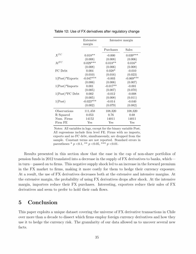
Table 12: Use of FX derivatives after regulatory change
Extensivemargin
Intensive margin
Purchases Sales
XTC 0.018** -0.000 0.039***(0.008) (0.008) (0.006)
MTC 0.029*** 0.018** 0.016*(0.008) (0.006) (0.008)
FC Debt 0.004 0.028* -0.010(0.010) (0.016) (0.023)
1(Post)*Exports -0.047*** -0.003 -0.069***(0.006) (0.006) (0.007)
1(Post)*Imports 0.001 -0.017** -0.001(0.005) (0.007) (0.070)
1(Post)*FC Debt 0.002 -0.012 -0.008(0.005) (0.008) (0.011)
1(Post) -0.023*** -0.014 -0.040(0.002) (0.079) (0.082)
Observations 111,458 108,320 108,320R Squared 0.053 0.76 0.68Num. Firms 14152 14011 14011Firm FE Yes Yes Yes
Notes: All variables in logs, except for the binary variable Post.All regressions include firm level FE. Firms with no imports,exports and no FC debt, simultaneously, are dropped from thesample. Constant terms are not reported. Standard errors inparentheses * p <0.1, ** p <0.05, *** p <0.01.
Results presented in this section show that the ease in the cap of non-share portfolios of
pension funds in 2012 translated into a decrease in the supply of FX derivatives to banks, which—
in turn—passed on to firms. This negative supply shock led to an increase in the forward premium
in the FX market to firms, making it more costly for them to hedge their currency exposure.
At a result, the use of FX derivatives decreases both at the extensive and intensive margins. At
the extensive margin, the probability of using FX derivatives drops after shock. At the intensive
margin, importers reduce their FX purchases. Interesting, exporters reduce their sales of FX
derivatives and seem to prefer to hold their cash flows.
5 Conclusion
This paper exploits a unique dataset covering the universe of FX derivative transactions in Chile
over more than a decade to dissect which firms employ foreign currency derivatives and how they
use it to hedge the currency risk. The granularity of our data allowed us to uncover several new
facts.
35
First, we showed that firms, even those that could exploit it further, are not “naturally
hedged”, as their receivables due to exports and payables due to imports are only marginally
correlated. Notably, this correlation remains small even when controlling for foreign currency
debt. We then assessed a plausible reason for low natural hedge: different maturity between
payables and receivables in foreign currency. We documented that indeed the trade credit for
imports has a much lower maturity than it has for exports, suggesting that it would actually be
very difficult for firms to be naturally hedged.
We then showed firms that employ FX derivatives to be larger and employ these instruments
to hedge larger transactions. We then assessed the use of FX derivatives at the extensive and
intensive margins. We found that, at both margins, trade credit for exports and imports associate
with a higher probability and use of FX derivatives. Interestingly, the size of the estimated
coefficients is rather small, which suggests that firms hedge a small part of the trade credit and
still have a large unhedged positions. Finally, we reported a maturity premium.
In the last section of the paper we used a reform that decreased the liquidity in the FX
derivative market for purchases purposes and showed that reduction in the supply of USD forward
substantially lowers the use of FX derivatives for hedging imports. This exercise suggests that
the more developed is the FX derivative market, the more firms would be able to hedge their
imports arguably limiting systemic risk associated to currency exposure.
36
References
Albagli, E., Calani, M., Hadzi-Vaskov, M., Marcel, M. and Ricci, L. A. (2020), Comfort in
floating: Taking stock of twenty years of freely-floating exchange rate in chile, IMF Working
Papers 20/100, International Monetary Fund.
Alfaro, L. and Chen, M. X. (2018), ‘Selection and market reallocation: Productivity gains from
multinational production’, American Economic Journal: Economic Policy 10(2), 1–38.
Alfaro, L., Garcia-Santana, M. and Moral-Benito, E. (2020), ‘On the direct and indirect real
effects of credit supply shocks’, Journal of Financial Economics forthcoming .
Alfonso-Corredor, V. A. (2018), ‘El uso de forwards peso dolar en las empresas colombianas del
sector real.’, Borradores de Economıa; No. 1058 .
Allayannis, G., Ihrig, J. and Weston, J. P. (2001), ‘Exchange-rate hedging: Financial versus
operational strategies’, American Economic Review 91(2), 391–395.
Amiti, M. and Weinstein, D. E. (2018), ‘How much do idiosyncratic bank shocks affect invest-
ment? evidence from matched bank-firm loan data’, Journal of Political Economy 126(2), 525–
587.
Antras, P. and Foley, C. F. (2015), ‘Poultry in motion: a study of international trade finance
practices’, Journal of Political Economy 123(4), 853–901.
Avalos, F. H. and Moreno, R. (2013), ‘Hedging in derivatives markets: the experience of chile’,
BIS Quarterly Review March .
Bae, S. C., Kim, H. S. and Kwon, T. H. (2018), ‘Currency derivatives for hedging: New evidence
on determinants, firm risk, and performance’, Journal of futures markets 38(4), 446–467.
Bekaert, G. and Hodrick, R. (2017), International financial management, Cambridge University
Press.
Bernard, A. B., Jensen, J. B., Redding, S. J. and Schott, P. K. (2007), ‘Firms in international
trade’, Journal of Economic Perspectives 21(3), 105–130.
Bruno, V. and Shin, H. S. (2015), ‘Capital flows and the risk-taking channel of monetary policy’,
Journal of Monetary Economics 71, 119–132.
Calvo, G. A. and Reinhart, C. M. (2002), ‘Fear of floating’, The Quarterly Journal of Economics
117(2), 379–408.
Cespedes, L. F., Chang, R. and Velasco, A. (2004), ‘Balance sheets and exchange rate policy’,
American Economic Review 94(4), 1183–1193.
37
Correa, R., Du, W. and Liao, G. Y. (2020), U.S. Banks and Global Liquidity, NBER Working
Papers 27491, National Bureau of Economic Research, Inc.
Du, W., Tepper, A. and Verdelhan, A. (2018), ‘Deviations from covered interest rate parity’, The
Journal of Finance 73(3), 915–957.
Eichengreen, B. and Hausmann, R. (1999), Exchange rates and financial fragility, Technical
report, National bureau of economic research.
Froot, K. A., Scharfstein, D. S. and Stein, J. C. (1993), ‘Risk management: Coordinating corpo-
rate investment and financing policies’, The Journal of Finance 48(5), 1629–1658.
Geczy, C., Minton, B. A. and Schrand, C. (1997), ‘Why firms use currency derivatives’, The
Journal of Finance 52(4), 1323–1354.
Goldberg, L. S. and Tille, C. (2016), ‘Micro, macro, and strategic forces in international trade
invoicing: Synthesis and novel patterns’, Journal of International Economics 102, 173–187.
Gopinath, G. (2015), The international price system, Technical report, National Bureau of Eco-
nomic Research.
Helpman, E., Melitz, M. J. and Yeaple, S. R. (2004), ‘Export versus fdi with heterogeneous
firms’, American economic review 94(1), 300–316.
Iacus, S. M., King, G. and Porro, G. (2012), ‘Causal inference without balance checking: Coars-
ened exact matching’, Political analysis pp. 1–24.
Ilzetzki, E., Reinhart, C. M. and Rogoff, K. S. (2019), ‘Exchange arrangements entering
the twenty-first century: Which anchor will hold?’, The Quarterly Journal of Economics
134(2), 599–646.
Khwaja, A. I. and Mian, A. (2008), ‘Tracing the impact of bank liquidity shocks: Evidence from
an emerging market’, American Economic Review 98(4), 1413–42.
Kuzmina, O. and Kuznetsova, O. (2018), ‘Operational and financial hedging: Evidence from
export and import behavior’, Journal of Corporate Finance 48, 109 – 121.
Liao, G. and Zhang, T. (2020), The hedging channel of exchange rate determination, Interna-
tional finance discussion paper 1283.
Lyonnet, V., Martin, J. and Mejean, I. (2016), Invoicing currency and financial hedging, CEPR
Discussion Papers 11700, C.E.P.R. Discussion Papers.
Melitz, M. J. (2003), ‘The impact of trade on intra-industry reallocations and aggregate industry
productivity’, Econometrica 71(6), 1695–1725.
38
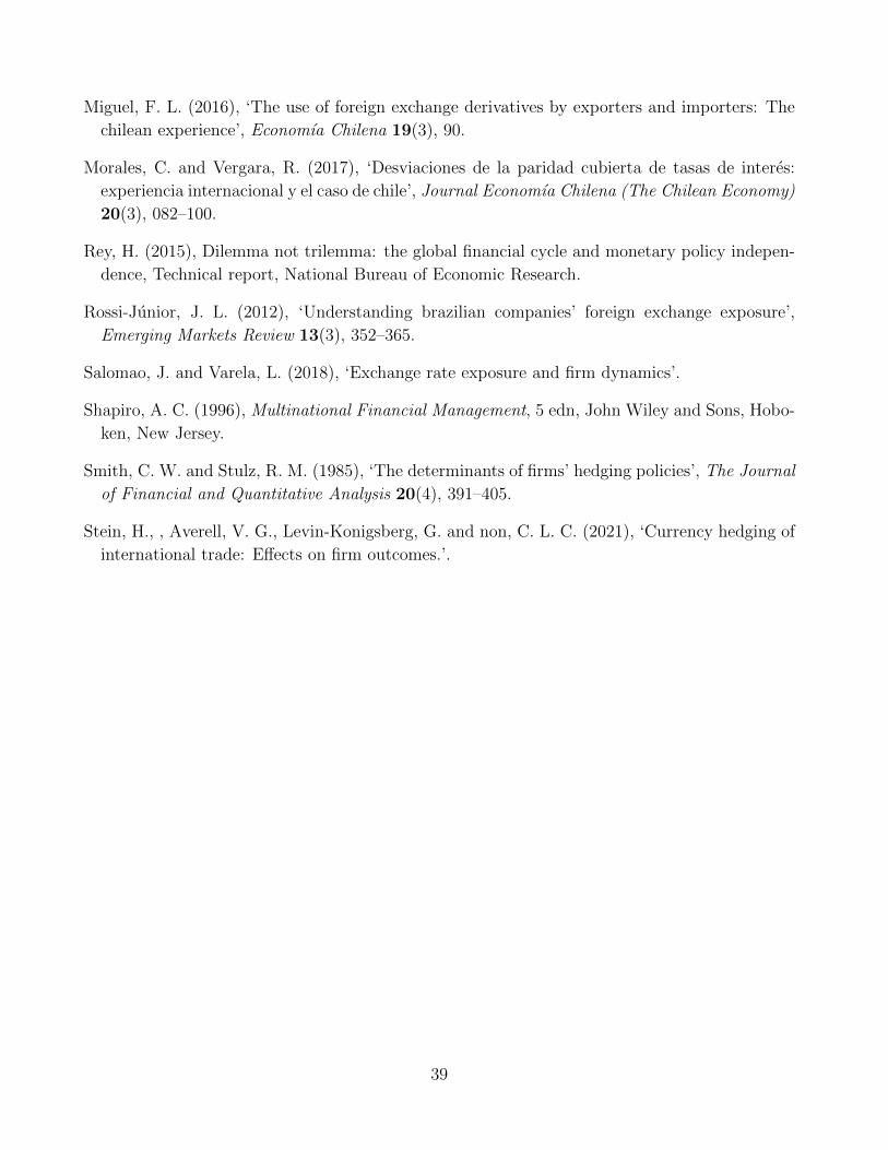
Miguel, F. L. (2016), ‘The use of foreign exchange derivatives by exporters and importers: The
chilean experience’, Economıa Chilena 19(3), 90.
Morales, C. and Vergara, R. (2017), ‘Desviaciones de la paridad cubierta de tasas de interes:
experiencia internacional y el caso de chile’, Journal Economıa Chilena (The Chilean Economy)
20(3), 082–100.
Rey, H. (2015), Dilemma not trilemma: the global financial cycle and monetary policy indepen-
dence, Technical report, National Bureau of Economic Research.
Rossi-Junior, J. L. (2012), ‘Understanding brazilian companies’ foreign exchange exposure’,
Emerging Markets Review 13(3), 352–365.
Salomao, J. and Varela, L. (2018), ‘Exchange rate exposure and firm dynamics’.
Shapiro, A. C. (1996), Multinational Financial Management, 5 edn, John Wiley and Sons, Hobo-
ken, New Jersey.
Smith, C. W. and Stulz, R. M. (1985), ‘The determinants of firms’ hedging policies’, The Journal
of Financial and Quantitative Analysis 20(4), 391–405.
Stein, H., , Averell, V. G., Levin-Konigsberg, G. and non, C. L. C. (2021), ‘Currency hedging of
international trade: Effects on firm outcomes.’.
39
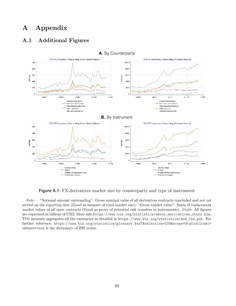
A Appendix
A.1 Additional Figures
A. By Counterparty
B. By Instrument
Figure A.1: FX-derivatives market size by counterparty and type of instrument
Note.— “Notional amount outstanding”: Gross nominal value of all derivatives contracts concluded and not yetsettled on the reporting date (Good as measure of total market size). “Gross market value”: Sums of replacementmarket values of all open contracts (Good as proxy of potential risk transfers in instruments). Units: All figuresare expressed in billions of USD. More info https://www.bis.org/statistics/about_derivatives_stats.htm.TO1 measure aggregates all the currencies as detailed in https://www.bis.org/statistics/dsd_lbs.pdf. Forfurther reference, https://www.bis.org/statistics/glossary.htm?&selection=209&scope=Statistics&c=
a&base=term is the dictionary of BIS terms.
40
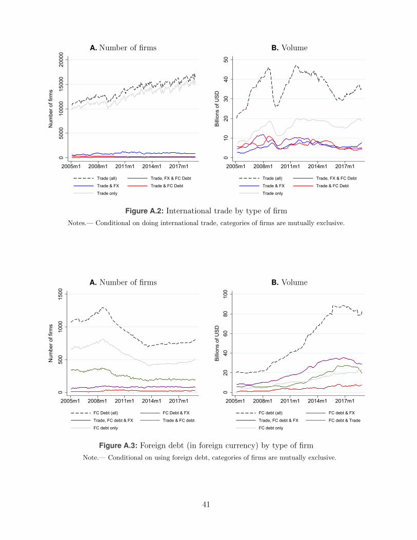
A. Number of firms
050
0010
000
1500
020
000
Num
ber o
f firm
s
2005m1 2008m1 2011m1 2014m1 2017m1
Trade (all) Trade, FX & FC Debt
Trade & FX Trade & FC Debt
Trade only
B. Volume
010
2030
4050
Billio
ns o
f USD
2005m1 2008m1 2011m1 2014m1 2017m1
Trade (all) Trade, FX & FC Debt
Trade & FX Trade & FC Debt
Trade only
Figure A.2: International trade by type of firm
Notes.— Conditional on doing international trade, categories of firms are mutually exclusive.
A. Number of firms
050
010
0015
00
Num
ber o
f firm
s
2005m1 2008m1 2011m1 2014m1 2017m1
FC Debt (all) FC Debt & FX
Trade, FC debt & FX Trade & FC debt
FC debt only
B. Volume
020
4060
8010
0Bi
llions
of U
SD
2005m1 2008m1 2011m1 2014m1 2017m1
FC debt (all) FC debt & FX
Trade, FC debt & FX FC debt & Trade
FC debt only
Figure A.3: Foreign debt (in foreign currency) by type of firm
Note.— Conditional on using foreign debt, categories of firms are mutually exclusive.
41
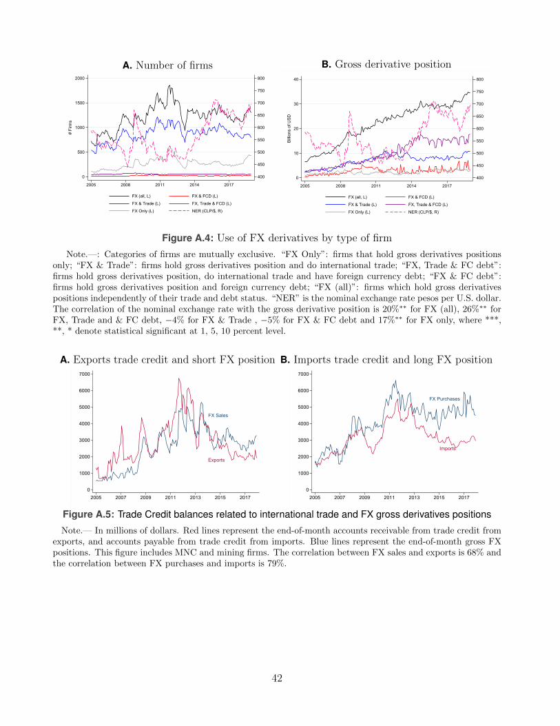
A. Number of firms
400
450
500
550
600
650
700
750
800
0
500
1000
1500
2000
# Fi
rms
2005 2008 2011 2014 2017
FX (all, L) FX & FCD (L)
FX & Trade (L) FX, Trade & FCD (L)
FX Only (L) NER (CLP/$, R)
B. Gross derivative position
400
450
500
550
600
650
700
750
800
0
10
20
30
40
Billio
ns o
f USD
2005 2008 2011 2014 2017
FX (all, L) FX & FCD (L)
FX & Trade (L) FX, Trade & FCD (L)
FX Only (L) NER (CLP/$, R)
Figure A.4: Use of FX derivatives by type of firm
Note.—: Categories of firms are mutually exclusive. “FX Only”: firms that hold gross derivatives positionsonly; “FX & Trade”: firms hold gross derivatives position and do international trade; “FX, Trade & FC debt”:firms hold gross derivatives position, do international trade and have foreign currency debt; “FX & FC debt”:firms hold gross derivatives position and foreign currency debt; “FX (all)”: firms which hold gross derivativespositions independently of their trade and debt status. “NER” is the nominal exchange rate pesos per U.S. dollar.The correlation of the nominal exchange rate with the gross derivative position is 20%∗∗ for FX (all), 26%∗∗ forFX, Trade and & FC debt, −4% for FX & Trade , −5% for FX & FC debt and 17%∗∗ for FX only, where ***,**, * denote statistical significant at 1, 5, 10 percent level.
A. Exports trade credit and short FX position
Exports
FX Sales
0
1000
2000
3000
4000
5000
6000
7000
2005 2007 2009 2011 2013 2015 2017
B. Imports trade credit and long FX position
Imports
FX Purchases
0
1000
2000
3000
4000
5000
6000
7000
2005 2007 2009 2011 2013 2015 2017
Figure A.5: Trade Credit balances related to international trade and FX gross derivatives positions
Note.— In millions of dollars. Red lines represent the end-of-month accounts receivable from trade credit fromexports, and accounts payable from trade credit from imports. Blue lines represent the end-of-month gross FXpositions. This figure includes MNC and mining firms. The correlation between FX sales and exports is 68% andthe correlation between FX purchases and imports is 79%.
42
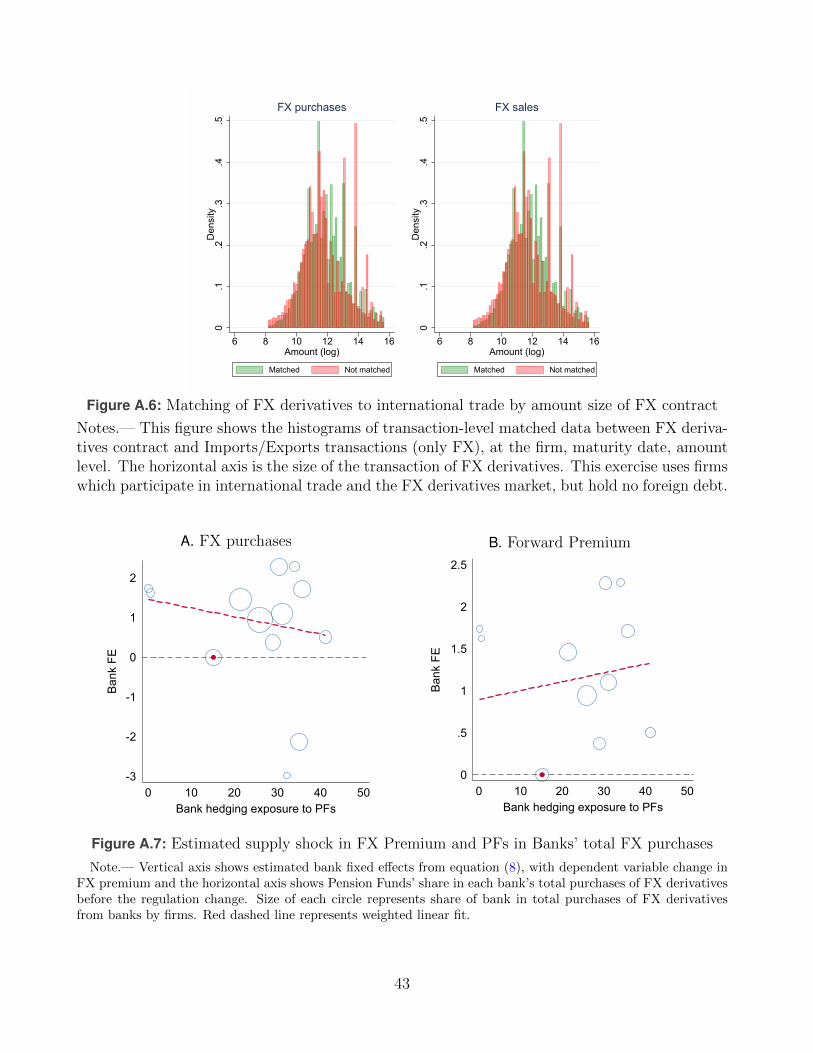
0.1
.2.3
.4.5
Den
sity
6 8 10 12 14 16Amount (log)
Matched Not matched
FX purchases
0.1
.2.3
.4.5
Den
sity
6 8 10 12 14 16Amount (log)
Matched Not matched
FX sales
Figure A.6: Matching of FX derivatives to international trade by amount size of FX contract
Notes.— This figure shows the histograms of transaction-level matched data between FX deriva-tives contract and Imports/Exports transactions (only FX), at the firm, maturity date, amountlevel. The horizontal axis is the size of the transaction of FX derivatives. This exercise uses firmswhich participate in international trade and the FX derivatives market, but hold no foreign debt.
A. FX purchases
-3
-2
-1
0
1
2
Bank
FE
0 10 20 30 40 50Bank hedging exposure to PFs
B. Forward Premium
0
.5
1
1.5
2
2.5
Bank
FE
0 10 20 30 40 50Bank hedging exposure to PFs
Figure A.7: Estimated supply shock in FX Premium and PFs in Banks’ total FX purchases
Note.— Vertical axis shows estimated bank fixed effects from equation (8), with dependent variable change inFX premium and the horizontal axis shows Pension Funds’ share in each bank’s total purchases of FX derivativesbefore the regulation change. Size of each circle represents share of bank in total purchases of FX derivativesfrom banks by firms. Red dashed line represents weighted linear fit.
43
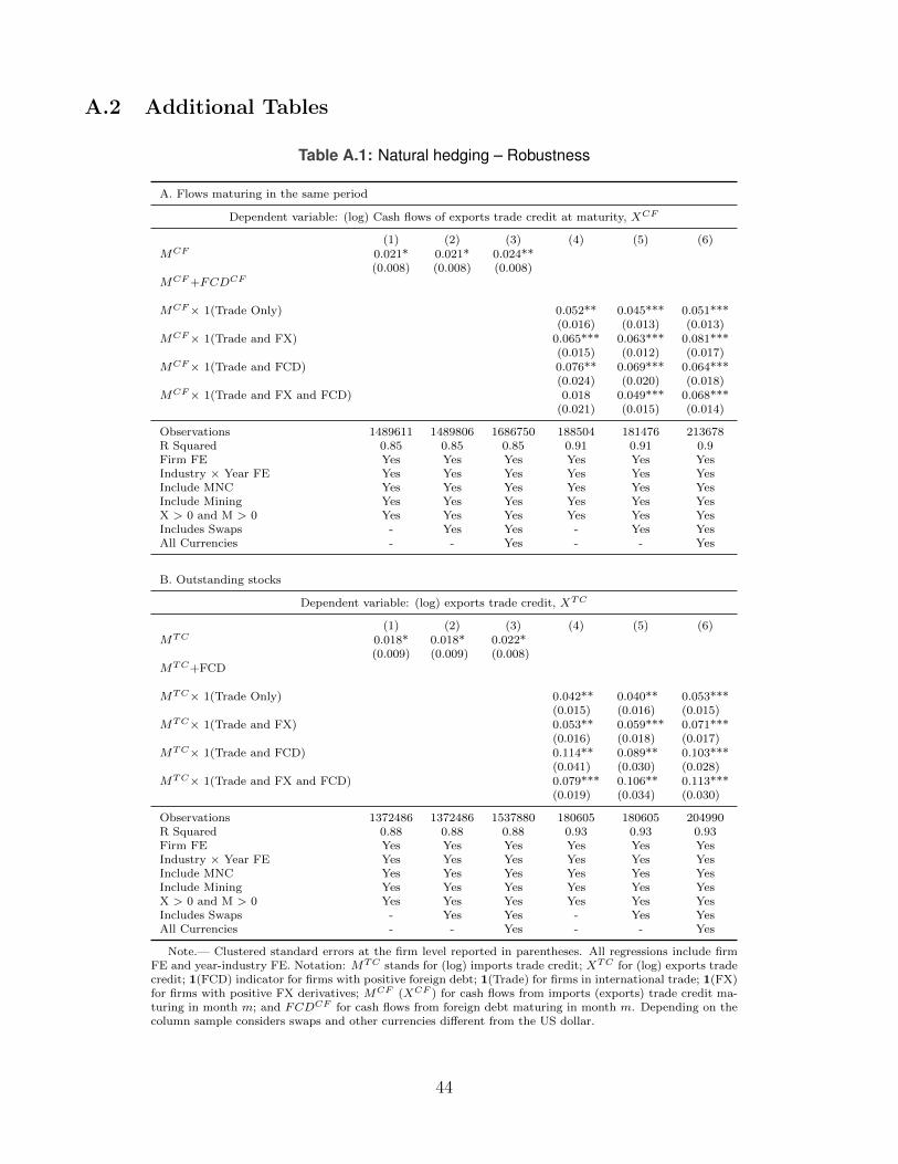
A.2 Additional Tables
Table A.1: Natural hedging – Robustness
A. Flows maturing in the same period
Dependent variable: (log) Cash flows of exports trade credit at maturity, XCF
(1) (2) (3) (4) (5) (6)MCF 0.021* 0.021* 0.024**
(0.008) (0.008) (0.008)MCF +FCDCF
MCF× 1(Trade Only) 0.052** 0.045*** 0.051***(0.016) (0.013) (0.013)
MCF× 1(Trade and FX) 0.065*** 0.063*** 0.081***(0.015) (0.012) (0.017)
MCF× 1(Trade and FCD) 0.076** 0.069*** 0.064***(0.024) (0.020) (0.018)
MCF× 1(Trade and FX and FCD) 0.018 0.049*** 0.068***(0.021) (0.015) (0.014)
Observations 1489611 1489806 1686750 188504 181476 213678R Squared 0.85 0.85 0.85 0.91 0.91 0.9Firm FE Yes Yes Yes Yes Yes YesIndustry × Year FE Yes Yes Yes Yes Yes YesInclude MNC Yes Yes Yes Yes Yes YesInclude Mining Yes Yes Yes Yes Yes YesX > 0 and M > 0 Yes Yes Yes Yes Yes YesIncludes Swaps - Yes Yes - Yes YesAll Currencies - - Yes - - Yes
B. Outstanding stocks
Dependent variable: (log) exports trade credit, XTC
(1) (2) (3) (4) (5) (6)MTC 0.018* 0.018* 0.022*
(0.009) (0.009) (0.008)MTC+FCD
MTC× 1(Trade Only) 0.042** 0.040** 0.053***(0.015) (0.016) (0.015)
MTC× 1(Trade and FX) 0.053** 0.059*** 0.071***(0.016) (0.018) (0.017)
MTC× 1(Trade and FCD) 0.114** 0.089** 0.103***(0.041) (0.030) (0.028)
MTC× 1(Trade and FX and FCD) 0.079*** 0.106** 0.113***(0.019) (0.034) (0.030)
Observations 1372486 1372486 1537880 180605 180605 204990R Squared 0.88 0.88 0.88 0.93 0.93 0.93Firm FE Yes Yes Yes Yes Yes YesIndustry × Year FE Yes Yes Yes Yes Yes YesInclude MNC Yes Yes Yes Yes Yes YesInclude Mining Yes Yes Yes Yes Yes YesX > 0 and M > 0 Yes Yes Yes Yes Yes YesIncludes Swaps - Yes Yes - Yes YesAll Currencies - - Yes - - Yes
Note.— Clustered standard errors at the firm level reported in parentheses. All regressions include firmFE and year-industry FE. Notation: MTC stands for (log) imports trade credit; XTC for (log) exports tradecredit; 1(FCD) indicator for firms with positive foreign debt; 1(Trade) for firms in international trade; 1(FX)for firms with positive FX derivatives; MCF (XCF ) for cash flows from imports (exports) trade credit ma-turing in month m; and FCDCF for cash flows from foreign debt maturing in month m. Depending on thecolumn sample considers swaps and other currencies different from the US dollar.
44
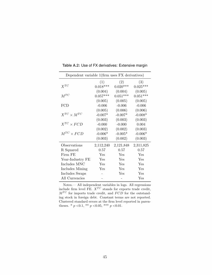
Table A.2: Use of FX derivatives: Extensive margin
Dependent variable 1(firm uses FX derivatives)
(1) (2) (3)XTC 0.018*** 0.020*** 0.025***
(0.004) (0.004) (0.005)MTC 0.057*** 0.051*** 0.051***
(0.005) (0.005) (0.005)FCD -0.006 -0.006 -0.006
(0.005) (0.006) (0.006)XTC ×MTC -0.007* -0.007* -0.008*
(0.003) (0.003) (0.003)XTC × FCD -0.000 -0.000 0.004
(0.002) (0.002) (0.003)MTC × FCD -0.006* -0.005* -0.006*
(0.003) (0.002) (0.003)
Observations 2,112,240 2,121,848 2,311,825R Squared 0.57 0.57 0.57Firm FE Yes Yes YesYear-Industry FE Yes Yes YesIncludes MNC Yes Yes YesIncludes Mining Yes Yes YesIncludes Swaps - Yes YesAll Currencies - - Yes
Notes.— All independent variables in logs. All regressionsinclude firm level FE. XTC stands for exports trade credit,MTC for imports trade credit, and FCD for the outstand-ing stock in foreign debt. Constant terms are not reported.Clustered standard errors at the firm level reported in paren-theses. * p <0.1, ** p <0.05, *** p <0.01.
45
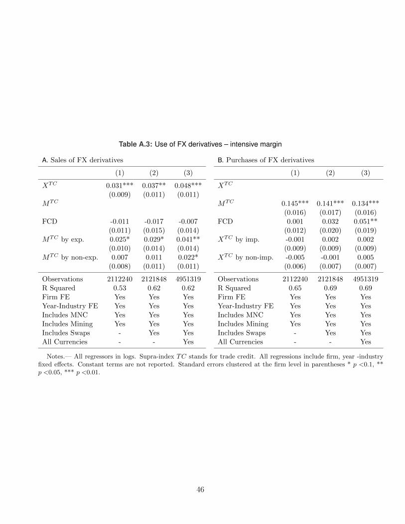
Table A.3: Use of FX derivatives – intensive margin
A. Sales of FX derivatives B. Purchases of FX derivatives
(1) (2) (3) (1) (2) (3)
XTC 0.031*** 0.037** 0.048*** XTC
(0.009) (0.011) (0.011)MTC MTC 0.145*** 0.141*** 0.134***
(0.016) (0.017) (0.016)FCD -0.011 -0.017 -0.007 FCD 0.001 0.032 0.051**
(0.011) (0.015) (0.014) (0.012) (0.020) (0.019)MTC by exp. 0.025* 0.029* 0.041** XTC by imp. -0.001 0.002 0.002
(0.010) (0.014) (0.014) (0.009) (0.009) (0.009)MTC by non-exp. 0.007 0.011 0.022* XTC by non-imp. -0.005 -0.001 0.005
(0.008) (0.011) (0.011) (0.006) (0.007) (0.007)
Observations 2112240 2121848 4951319 Observations 2112240 2121848 4951319R Squared 0.53 0.62 0.62 R Squared 0.65 0.69 0.69Firm FE Yes Yes Yes Firm FE Yes Yes YesYear-Industry FE Yes Yes Yes Year-Industry FE Yes Yes YesIncludes MNC Yes Yes Yes Includes MNC Yes Yes YesIncludes Mining Yes Yes Yes Includes Mining Yes Yes YesIncludes Swaps - Yes Yes Includes Swaps - Yes YesAll Currencies - - Yes All Currencies - - Yes
Notes.— All regressors in logs. Supra-index TC stands for trade credit. All regressions include firm, year -industryfixed effects. Constant terms are not reported. Standard errors clustered at the firm level in parentheses * p <0.1, **p <0.05, *** p <0.01.
46
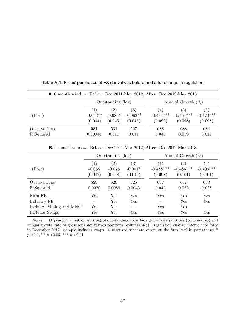
Table A.4: Firms’ purchases of FX derivatives before and after change in regulation
A. 6 month window. Before: Dec 2011-May 2012, After: Dec 2012-May 2013
Outstanding (log) Annual Growth (%)
(1) (2) (3) (4) (5) (6)1(Post) -0.093** -0.089* -0.093** -0.481*** -0.464*** -0.470***
(0.044) (0.045) (0.046) (0.095) (0.098) (0.098)
Observations 531 531 527 688 688 684R Squared 0.00044 0.011 0.011 0.040 0.019 0.019
B. 4 month window. Before: Dec 2011-Mar 2012, After: Dec 2012-Mar 2013
Outstanding (log) Annual Growth (%)
(1) (2) (3) (4) (5) (6)1(Post) -0.068 -0.076 -0.081* -0.488*** -0.486*** -0.496***
(0.047) (0.048) (0.049) (0.098) (0.101) (0.101)
Observations 529 529 525 657 657 653R Squared 0.0020 0.0089 0.0046 0.046 0.022 0.023
Firm FE Yes Yes Yes Yes Yes YesIndustry FE – Yes Yes – Yes YesIncludes Mining and MNC Yes Yes — Yes Yes —Includes Swaps Yes Yes Yes Yes Yes Yes
Notes.— Dependent variables are (log) of outstanding gross long derivatives positions (columns 1-3) andannual growth rate of gross long derivatives positions (columns 4-6). Regulation change entered into forcein December 2012. Sample includes swaps. Clusterized standard errors at the firm level in parentheses *p <0.1, ** p <0.05, *** p <0.01
47
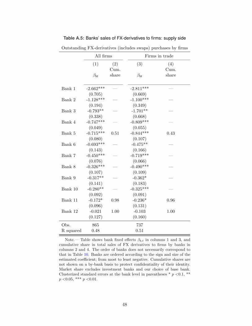
Table A.5: Banks’ sales of FX-derivatives to firms: supply side
Outstanding FX-derivatives (includes swaps) purchases by firms
All firms Firms in trade
(1) (2) (3) (4)Cum. Cum.
βbt share βbt share
Bank 1 -2.662*** — -2.811*** —(0.705) (0.669)
Bank 2 -1.128*** — -1.100*** —(0.194) (0.349)
Bank 3 -0.793** — -1.701** —(0.338) (0.668)
Bank 4 -0.747*** — -0.809*** —(0.049) (0.055)
Bank 5 -0.715*** 0.51 -0.844*** 0.43(0.080) (0.107)
Bank 6 -0.693*** — -0.475** —(0.143) (0.166)
Bank 7 -0.450*** — -0.719*** —(0.076) (0.066)
Bank 8 -0.326*** — -0.490*** —(0.107) (0.109)
Bank 9 -0.317** — -0.362* —(0.141) (0.183)
Bank 10 -0.280** — -0.325*** —(0.092) (0.091)
Bank 11 -0.172* 0.98 -0.236* 0.96(0.096) (0.131)
Bank 12 -0.021 1.00 -0.103 1.00(0.127) (0.160)
Obs. 865 737R squared 0.48 0.51
Note.— Table shows bank fixed effects βb,t in columns 1 and 3, andcumulative share in total sales of FX derivatives to firms by banks incolumns 2 and 4. The order of banks does not necessarily correspond tothat in Table 10. Banks are ordered according to the sign and size of theestimated coefficient; from most to least negative. Cumulative shares arenot shown on a by-bank basis to protect confidentiality of their identity.Market share excludes investment banks and our choice of base bank.Clusterized standard errors at the bank level in parentheses * p <0.1, **p <0.05, *** p <0.01.
48
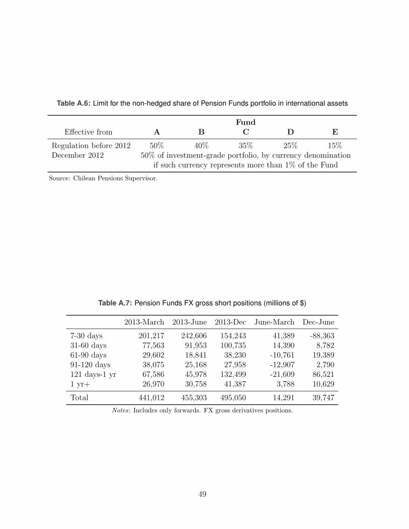
Table A.6: Limit for the non-hedged share of Pension Funds portfolio in international assets
FundEffective from A B C D E
Regulation before 2012 50% 40% 35% 25% 15%December 2012 50% of investment-grade portfolio, by currency denomination
if such currency represents more than 1% of the Fund
Source: Chilean Pensions Supervisor.
Table A.7: Pension Funds FX gross short positions (millions of $)
2013-March 2013-June 2013-Dec June-March Dec-June
7-30 days 201,217 242,606 154,243 41,389 -88,36331-60 days 77,563 91,953 100,735 14,390 8,78261-90 days 29,602 18,841 38,230 -10,761 19,38991-120 days 38,075 25,168 27,958 -12,907 2,790121 days-1 yr 67,586 45,978 132,499 -21,609 86,5211 yr+ 26,970 30,758 41,387 3,788 10,629
Total 441,012 455,303 495,050 14,291 39,747
Notes: Includes only forwards. FX gross derivatives positions.
49
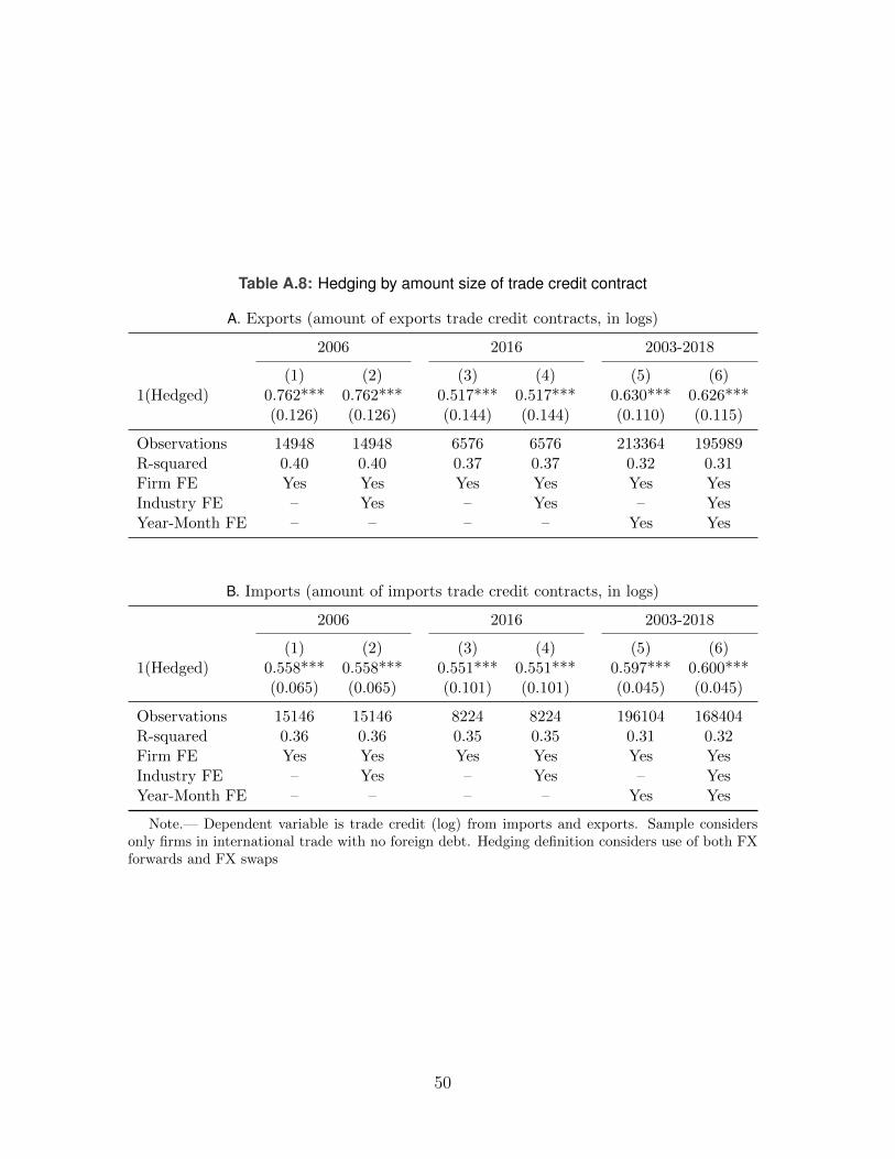
Table A.8: Hedging by amount size of trade credit contract
A. Exports (amount of exports trade credit contracts, in logs)
2006 2016 2003-2018
(1) (2) (3) (4) (5) (6)1(Hedged) 0.762*** 0.762*** 0.517*** 0.517*** 0.630*** 0.626***
(0.126) (0.126) (0.144) (0.144) (0.110) (0.115)
Observations 14948 14948 6576 6576 213364 195989R-squared 0.40 0.40 0.37 0.37 0.32 0.31Firm FE Yes Yes Yes Yes Yes YesIndustry FE – Yes – Yes – YesYear-Month FE – – – – Yes Yes
B. Imports (amount of imports trade credit contracts, in logs)
2006 2016 2003-2018
(1) (2) (3) (4) (5) (6)1(Hedged) 0.558*** 0.558*** 0.551*** 0.551*** 0.597*** 0.600***
(0.065) (0.065) (0.101) (0.101) (0.045) (0.045)
Observations 15146 15146 8224 8224 196104 168404R-squared 0.36 0.36 0.35 0.35 0.31 0.32Firm FE Yes Yes Yes Yes Yes YesIndustry FE – Yes – Yes – YesYear-Month FE – – – – Yes Yes
Note.— Dependent variable is trade credit (log) from imports and exports. Sample considersonly firms in international trade with no foreign debt. Hedging definition considers use of both FXforwards and FX swaps
50
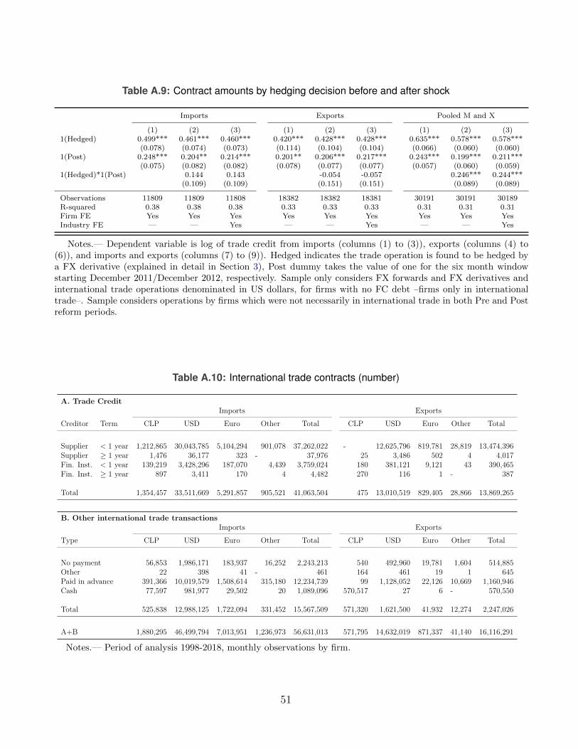
Table A.9: Contract amounts by hedging decision before and after shock
Imports Exports Pooled M and X
(1) (2) (3) (1) (2) (3) (1) (2) (3)1(Hedged) 0.499*** 0.461*** 0.460*** 0.420*** 0.428*** 0.428*** 0.635*** 0.578*** 0.578***
(0.078) (0.074) (0.073) (0.114) (0.104) (0.104) (0.066) (0.060) (0.060)1(Post) 0.248*** 0.204** 0.214*** 0.201** 0.206*** 0.217*** 0.243*** 0.199*** 0.211***
(0.075) (0.082) (0.082) (0.078) (0.077) (0.077) (0.057) (0.060) (0.059)1(Hedged)*1(Post) 0.144 0.143 -0.054 -0.057 0.246*** 0.244***
(0.109) (0.109) (0.151) (0.151) (0.089) (0.089)
Observations 11809 11809 11808 18382 18382 18381 30191 30191 30189R-squared 0.38 0.38 0.38 0.33 0.33 0.33 0.31 0.31 0.31Firm FE Yes Yes Yes Yes Yes Yes Yes Yes YesIndustry FE — — Yes — — Yes — — Yes
Notes.— Dependent variable is log of trade credit from imports (columns (1) to (3)), exports (columns (4) to(6)), and imports and exports (columns (7) to (9)). Hedged indicates the trade operation is found to be hedged bya FX derivative (explained in detail in Section 3), Post dummy takes the value of one for the six month windowstarting December 2011/December 2012, respectively. Sample only considers FX forwards and FX derivatives andinternational trade operations denominated in US dollars, for firms with no FC debt –firms only in internationaltrade–. Sample considers operations by firms which were not necessarily in international trade in both Pre and Postreform periods.
Table A.10: International trade contracts (number)
A. Trade CreditImports Exports
Creditor Term CLP USD Euro Other Total CLP USD Euro Other Total
Supplier < 1 year 1,212,865 30,043,785 5,104,294 901,078 37,262,022 - 12,625,796 819,781 28,819 13,474,396Supplier ≥ 1 year 1,476 36,177 323 - 37,976 25 3,486 502 4 4,017Fin. Inst. < 1 year 139,219 3,428,296 187,070 4,439 3,759,024 180 381,121 9,121 43 390,465Fin. Inst. ≥ 1 year 897 3,411 170 4 4,482 270 116 1 - 387
Total 1,354,457 33,511,669 5,291,857 905,521 41,063,504 475 13,010,519 829,405 28,866 13,869,265
B. Other international trade transactionsImports Exports
Type CLP USD Euro Other Total CLP USD Euro Other Total
No payment 56,853 1,986,171 183,937 16,252 2,243,213 540 492,960 19,781 1,604 514,885Other 22 398 41 - 461 164 461 19 1 645Paid in advance 391,366 10,019,579 1,508,614 315,180 12,234,739 99 1,128,052 22,126 10,669 1,160,946Cash 77,597 981,977 29,502 20 1,089,096 570,517 27 6 - 570,550
Total 525,838 12,988,125 1,722,094 331,452 15,567,509 571,320 1,621,500 41,932 12,274 2,247,026
A+B 1,880,295 46,499,794 7,013,951 1,236,973 56,631,013 571,795 14,632,019 871,337 41,140 16,116,291
Notes.— Period of analysis 1998-2018, monthly observations by firm.
51
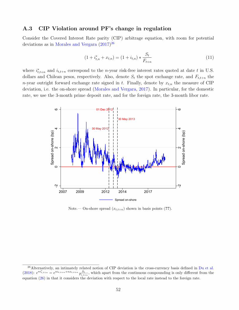
A.3 CIP Violation around PF’s change in regulation
Consider the Covered Interest Rate parity (CIP) arbitrage equation, with room for potential
deviations as in Morales and Vergara (2017)26
(1 + i∗t,n + xt,n) = (1 + it,n) ∗ StFt+n
(11)
where i∗t,t+n and it,t+n correspond to the n-year risk-free interest rates quoted at date t in U.S.
dollars and Chilean pesos, respectively. Also, denote St the spot exchange rate, and Ft,t+n the
n-year outright forward exchange rate signed in t. Finally, denote by xt,n the measure of CIP
deviation, i.e. the on-shore spread (Morales and Vergara, 2017). In particular, for the domestic
rate, we use the 3-month prime deposit rate, and for the foreign rate, the 3-month libor rate.
01 Dec 2012
30 May 2013
30 May 2012
-20
24
6Sp
read
on-
shor
e (b
p)
-20
24
6Sp
read
on-
shor
e (b
p)
2007 2009 2012 2014 2017
Spread on-shore
Note.— On-shore spread (xt,t+n) shown in basis points (??).
26Alternatively, an intimately related notion of CIP deviation is the cross-currency basis defined in Du et al.(2018): eni
∗t,t+n = enit,t+n+nxt,t+n St
Ft,t+n, which apart from the continuous compounding is only different from the
equation (26) in that it considers the deviation with respect to the local rate instead to the foreign rate.
52