Cupid’s Invisible Hand:

Social Surplus and Identification in Matching Models

Alfred Galichon1 Bernard Salanie2

September 17, 20123

1Economics Department, Sciences Po, Paris; e-mail: alfred.galichon@sciences-po.fr2Department of Economics, Columbia University; e-mail: bsalanie@columbia.edu.3The authors are grateful to Pierre-Andre Chiappori, Chris Conlon, Jim Heckman, Robert Mc-

Cann, Jean-Marc Robin, and many seminar participants for useful comments and discussions. Gali-

chon gratefully acknowledges support from Chaire “Assurance et Risques Majeurs” and FiME,

Laboratoire de Finance des Marches de l’Energie. Part of the research underlying this paper was

done when Galichon was visiting the University of Chicago Booth School of Business and Columbia

University, and when Salanie was visiting the Toulouse School of Economics. Galichon thanks the

Alliance program for its support, and Salanie thanks the Georges Meyer endowment.

Abstract

We investigate a model of one-to-one matching with transferable utility when some of the

characteristics of the players are unobservable to the analyst. We allow for a wide class of

distributions of unobserved heterogeneity, subject only to a separability assumption that

generalizes Choo and Siow (2006). We first show that the stable matching maximizes a social

gain function that trades off the average surplus due to the observable characteristics and a

generalized entropy term that reflects the impact of matching on unobserved characteristics.

We use this result to derive simple closed-form formulæ that identify the joint surplus in

every possible match and the equilibrium utilities of all participants, given any known

distribution of unobserved heterogeneity. If transfers are observed, then the pre-transfer

utilities of both partners are also identified. We also present a very fast algorithm that

computes the optimal matching for any specification of the joint surplus. We conclude by

discussing some empirical approaches suggested by these results.

Keywords: matching, marriage, assignment, hedonic prices.

JEL codes: C78, D61, C13.

Introduction

Since the seminal contribution of Becker (1973), economists have modeled the marriage

market as a matching problem in which each potential match generates a marital surplus.

Given transferable utilities, the distributions of tastes and of desirable characteristics de-

termine equilibrium shadow prices, which in turn explain how partners share the marital

surplus in any realized match. This insight is not specific of the marriage market: it char-

acterizes the “assignment game” (Shapley and Shubik 1972), i.e. models of matching with

transferable utilities. These models have also been applied to competitive equilibrium with

hedonic pricing (Chiappori, McCann, and Nesheim 2010) and the market for CEOs (Tervio

(2008) and Gabaix and Landier (2008).) We will show how our results can be used in these

three contexts; but for concreteness, we often refer to partners as men and women in the

exposition of the main results.

While Becker presented the general theory, he focused on the special case in which the

types of the partners are one-dimensional and are complementary in producing surplus.

As is well-known, the socially optimal matches then exhibit positive assortative matching :

higher types pair up with higher types, and lower types with lower types. Moreover, the

resulting configuration is stable, it is in the core of the corresponding matching game, and

it can be efficiently implemented by classical optimal assignment algorithms.

This sorting result is both simple and powerful; but its implications are also quite

unrealistic and at variance with the data, in which matches are observed between partners

with quite different characteristics. To account for this wider variety of matching patterns,

one could introduce search frictions, as in Shimer and Smith (2000) or Jacquemet and Robin

(2011). But the resulting model is hard to handle, and under some additional conditions

it still implies assortative matching. An alternative solution consists in allowing the joint

surplus of a match to incorporate latent characteristics—heterogeneity that is unobserved

by the analyst. Choo and Siow (2006) showed that it can be done in a way that yields a

highly tractable model in large populations, provided that the unobserved heterogeneities

enter the marital surplus quasi-additively and that they are distributed as standard type I

1

extreme value terms. Then the usual apparatus of multinomial logit discrete choice models

applies, linking marriage patterns to marital surplus in a very simple manner. Choo and

Siow (2006) used this model to link the changes in gains to marriage and abortion laws;

Siow and Choo (2006) applied it to Canadian data to measure the impact of demographic

changes. It has also been used to study increasing returns in marriage markets (Botticini

and Siow 2008) and to test for complementarities across partner educations (Siow 2009);

and, in a heteroskedastic version, to estimate the changes in the returns to education on

the US marriage market (Chiappori, Salanie, and Weiss 2012).

We revisit here the theory of matching with transferable utilities in the light of Choo and

Siow’s insights; and we extend this framework to quite general distributions of unobserved

variations in tastes. Our main contributions are twofold. First, we prove that the optimal

matching maximizes a very simple function of the observable only. With quasi-additive

surplus, the market equilibrium maximizes a social surplus function that consists of two

terms: a term that describes assortativeness on the observed characteristics; and a general-

ized entropic term that describes the random character of matching conditional on observed

characteristics. While the first term tends to match partners with complementary observed

characteristics, the second one pulls towards randomly assigning partners to each other.

The social gain from any matching patterns trades off these two terms. In particular, when

unobserved heterogeneity is distributed as in Choo and Siow (2006), the generalized entropy

is simply the usual entropy measure. The maximization of this social surplus function has

very straightforward consequences in terms of identification, both when equilibrium trans-

fers are observed and when they are not. In fact, most quantities of interest can be obtained

from derivatives of the terms that constitute generalized entropy. We show in particular

that the joint surplus from matching is (minus) a derivative of the generalized entropy,

computed at the observed matching. The expected and realized utilities of all types of men

and women follow just as directly. If moreover equilibrium transfers are observed, then we

also identify the pre-transfer utilities on both sides of the market. To prove these results,

we combine tools from duality and convexity theory, and we construct the Legendre-Fenchel

2

transform of the expected utilities of agents. A similar approach was used independently

by Decker, Lieb, McCann, and Stephens (2012) to prove the uniqueness of the equilibrium

and derive some of its properties in the Choo and Siow framework.

Our second contribution is to delineate an empirical approach to parametric estimation

in this class of models, using maximum likelihood. Indeed, our nonparametric identification

results rely on the strong assumption that the distribution of the unobservables is known,

while in practice the analyst will want to estimate its parameters. The large number of

covariates available to model the surplus function also limits the scope of nonparametric

estimation. Maximum likelihood estimation is thus a natural recourse; but since evaluating

the likelihood requires solving for the optimal matching, computational considerations loom

large in matching models. We provide an efficient algorithm that maximizes the social

surplus for any joint surplus function and computes the optimal matching, as well as the

expected utilities in equilibrium. To do this, we adapt the Iterative Projection Fitting

Procedure (known to some economists as RAS) to the structure of this problem. IPFP

is a very stable and very simple algorithm; we report simulations that show that is much

faster than alternative solvers. Finally, we show that in the context of the Choo and Siow

(2006) model the maximum likelihood is a simple moment matching estimator, and we give

a geometric interpretation.

There are other approaches to estimating matching models with unobserved hetero-

geneity; see the handbook chapter by Graham (2011). Fox (2010) in particular exploits

a “rank-order property” and pools data across many similar markets; see Fox (2011) and

Bajari and Fox (2009) for applications. More recently, Fox and Yang (2012) focus on iden-

tifying the complementarity between unobservable characteristics. We discuss the pros and

cons of various methods in our conclusion.

Section 1 sets up the model and the notation. We prove our main results in Section 2,

and we specialize them to leading examples in Section 3. Our results open the way to

new and richer specifications; Section 4 explains how to estimate them using maximum

likelihood, and how to use various restrictions to identify the underlying parameters. We

3

present in Section 5 our IPFP algorithm, which greatly accelerates computations. Finally,

Section 6 specializes our results to a restricted but useful model1.

1 The Assignment Problem with Unobserved Heterogeneity

1.1 The Populations

Throughout the paper, we maintain the basic assumptions of the transferable utility model

of Choo and Siow (2006): utility transfers between partners are unconstrained, matching

is frictionless, and there is no asymmetric information among potential partners. We call

the partners “men” and “women”, but our results are clearly not restricted to the marriage

market.

Men are denoted by i ∈ I and women by j ∈ J . A matching (µij) is a matrix such that

µij = 1 if man i and woman j are matched, 0 otherwise. A matching is feasible if for every

i and j, ∑k∈J

µik ≤ 1 and∑k∈I

µkj ≤ 1,

with equality for individuals who are married. Single individuals are “matched with 0”:

µi0 = 1 or µ0j = 1. For completeness, we should add the requirement that µij is integral

(µij ∈ {0, 1}). However it is known since at least Shapley and Shubik (1972) that this

constraint is not binding, so we will omit it.

A hypothetical match between man i and woman j allows them to share a total utility

Φij ; the division of this total utility between them is done through utility transfers whose

value is determined in equilibrium. Singles get utilities Φi0, Φ0j . Following Gale and Shapley

(1962) for matching with non-transferable utility, we focus on the set of stable matchings.

A feasible matching is stable if there exists a division of the surplus in each realized match

that makes it impossible for any man k and woman l to both achieve strictly higher utility

by pairing up together, and for any agent to achieve higher utility by being single. More

1This paper builds on and significantly extends our earlier discussion paper (Galichon and Salanie 2010),

which is now obsolete.

4

formally, let ui denote the utility man i gets in his current match; denote vj the correspond-

ing utilities for woman j. Then by definition ui + vj = Φij if they are matched, that is if

µij > 0; and ui = Φi0 (resp. vj = Φ0j) if i (resp. j) is single. Stability requires that for

every man k and woman l, uk ≥ Φk0 and vl ≥ Φ0l, and uk + vl ≥ Φkl for any potential

match (k, l).

Finally, a competitive equilibrium is defined as a set of prices ui and vj and a feasible

matching µij such that

µij > 0 iff j ∈ arg maxj∈J∪{0}

(Φij − vj

)and i ∈ arg max

i∈I∪{0}

(Φij − ui

). (1.1)

Shapley and Shubik (1972) showed that the set of stable matchings coincides with the set

of competitive equilibria (and with the core of the assignment game); and that moreover,

any stable matching achieves the maximum of the total surplus2

∑i∈I

∑j∈J

νijΦij +∑i∈I

νi0Φi0 +∑j∈J

ν0jΦ0j

over all feasible matchings ν.

The set of stable matchings is generically a singleton; on the other hand, the set of prices

ui and vj (or, equivalently, the division of the surplus into ui and vj) that support it is a

product of intervals.

1.2 Groups

The analyst only observes some of the payoff-relevant characteristics that determine the

surplus matrix Φ. Following Choo and Siow (2006), we assume that she can only observe

which group each individual belongs to. Each man i ∈ I belongs to one group xi ∈ X ;

and, similarly, each woman j ∈ J belongs to one group yj ∈ Y. Groups are defined by the

intersection of characteristics which are observed by all men and women, and also by the

analyst. On the other hand, men and women of a given group differ along some dimensions

that they all observe, but which do not figure in the analyst’s dataset.

2See also Gretsky, Ostroy, and Zame (1992) for the extension to a continuum of agents.

5

As an example, observed groups x, y = (E,R) may consist of education and income.

Education could take values E ∈ {D,G} (dropout or graduate), and income class R could

take values 1 to nR. Groups may also incorporate information that is sometimes available

to the econometrician, such as physical characteristics, religion, and so on. In this paper

we take the numbers of groups |X | and |Y| to be finite in number; we return to the case of

continuous groups in the conclusion.

We denote nx the number of men in group x, and my the number of women in group

y. Like Choo and Siow, we assume that there are a large number of men in any group x,

and of women in any group y. More precisely, our statements in the following hold exactly

when the number of individuals goes to infinity and the proportions of genders and groups

converge. To simplify the exposition, we consider the limit of a sequence of large economies

where the proportion of each group remains constant:

Assumption 1 (Large Market) The number of individuals on the market

N =∑x∈X

nx +∑y∈Y

my

goes to infinity; and the ratios (nx/N) and (my/N) are constant.

With finite N we would need to introduce corrective terms; however, since N is the size

of the total population rather than that of the sample we use for estimation, these terms

can safely be neglected in applications to the marriage market for instance.

Another benefit of Assumption 1 is that it mitigates concerns about agents misrepresent-

ing their characteristics. This is almost always a profitable deviation in finite populations;

but as shown by Gretsky, Ostroy, and Zame (1999), the benefit from such manipulations

goes to zero as the population is replicated. In the large markets limit, the equilibrium

prices ui and vj are unique. We will therefore write “the equilibrium” in what follows.

The analyst does not observe some of the characteristics of the players, and she can only

compute quantities that depend on the observed groups of the partners in a match. Hence

she cannot observe µ, and she must focus instead on the matrix of matches across groups

6

(µxy). This is related to (µij) by

µxy =∑i,j

11 (xi = x, yj = y) µij

with the obvious extension to µx0 and µ0y.

The feasibility constraints on µxy ≥ 0 are

∀x ∈ X ,∑y∈Y

µxy ≤ nx ; ∀y ∈ Y,∑x∈X

µxy ≤ my (1.2)

which simply means that the number of married men (women) of group x (y) is not greater

than the number of men (women) of group x (y). For future reference, we denoteM the set

of (|X | |Y|+ |X |+ |Y|) non-negative numbers (µxy) that satisfy these (|X |+ |Y|) equalities.

Each element ofM is called a “matching” as it defines a feasible set of matches (and singles).

For notational convenience, we shall denote µx0 the number of single men of group x and

µ0y the number of single women of group y, and X0 = X ∪ {0} and Y0 = Y ∪ {0} the set of

marital choices that are available to agents, including singlehood. Obviously,

µx0 = nx −∑y∈Y

µxy and µ0y = my −∑x∈X

µxy.

1.3 Matching Surpluses

Several approaches can be used to take this model to the data. A “brute force” method

would use a parametric specification for the surplus Φmw and solve the system of equilibrium

equations (1.1). The set of maximizers at the solution of this system defines the stable

matchings, and can be compared to the observed matching in order to derive a minimum

distance estimator of the parameters. However, there are two problems with this approach:

it is very costly, and it is not clear at all what drives identification of the parameters. The

literature has instead attempted to impose identifying assumptions that allow for more

transparent identification. We follow here the framework of Choo and Siow (2006). We will

7

discuss other approaches in the conclusion, including those of Fox (2010) and Fox and Yang

(2012).

Choo and Siow assumed that the utility surplus of a man i of group x (that is, such

that xi = x) who marries a woman of group y can be written as

αxy + τ + εiy, (1.3)

where αxy is the systematic part of the surplus τ represents the utility transfer (possibly

negative) that the man gets from his partner in equilibrium, and εiy is a standard type I

extreme value random variation. If such a man remains single, he gets utility εi0; that is to

say, the systematic utilities of singles αx0 are normalized to zero. Similarly, the utility of a

woman j of group yj = y who marries a man of group x can be written as

γxy − τ + ηxj , (1.4)

where τ is the utility transfer she leaves to her partner. A woman of group y gets utility

η0j if she is single, that is we adopt normalization γ0y = 0.

As shown in Chiappori, Salanie, and Weiss (2012), the key assumption here is that the

joint surplus created when a man i of group x marries a woman j of group y rule out

interactions between their unobserved characteristics, conditional on (x, y). This leads us

to assume:

Assumption 2 (Separability) There exists a vector Φxy such that the joint surplus from

a match between a man i in group x and a woman j in group j is

Φij = Φxy + εiy + ηxj .

In Choo and Siow’s formulation, the vector Φ is simply

Φxy = αxy + γxy,

which they call the total systematic net gains to marriage; and note that by construction,

Φx0 and Φ0y are zero. It is easy to see that Assumption 2 is equivalent to specifying that if

8

two men i and i′ belong to the same group x, and their respective partners j and j′ belong

to the same group y, then the total surplus generated by these two matches is unchanged if

we shuffle partners: Φij+Φi′j′ = Φij′+Φi′j . Note that in this form it is clear that we needn’t

adopt Choo and Siow’s original interpretation of ε as a preference shock of the husband and

η as a preference shock of the wife. To take an extreme example, we could equally have men

who are indifferent over partners and are only interested in the transfer they receive, so that

their ex post utility is τ ; and women who also care about some attractiveness characteristic

of men, in a way that may depend on the woman’s group. The net utility of women of

group y would be εiy − τ ; the resulting joint surplus would satisfy Assumption 2 and all of

our results would apply3. In other words, there is no need to assume that the term εiyj was

“created” by man i, nor that the term ηjxi was “created” by the woman j; it may perfectly

be the opposite.

1.4 Choo and Siow’s Identification Result

In addition to Assumptions 1 and 2, Choo and Siow (2006) specified the distribution of

unobserved heterogeneities to be independent products of standard type I extreme values

distributions:

Assumption 3 (Type-I extreme values distribution)

a) For any man i, the (εiy)y∈Y0 are drawn independently from a standard type I extreme

value distribution;

b) For any woman j, the (ηxj)x∈X0 are drawn independently from a standard type I

extreme value distribution;

c) These draws are independent across men and women.

3It is easy to see that in such a model, a man i who is married in equilibrium is matched with a woman

in the group that values his attractiveness most, and he receives a transfer τ i = maxy∈Y εiy.

9

Choo and Siow proved that under Assumptions 1-3, there is a simple equilibrium re-

lationship between group preferences, as defined by α and γ, and equilibrium marriage

patterns. To state their result, we denote µxy the number of marriages between men of

group x and women of group y; µx0 the number of single men of group x; and µ0y the

number of single women of group y. Then:

Theorem 1 (Choo and Siow) Under Assumptions 1-3, in equilibrium, for all x, y ≥ 1

exp

(Φxy

2

)=

µxy√µx0µ0y

.

Therefore marriage patterns µ directly identify the gains to marriage Φ.

1.5 Unobserved Heterogeneity

One of our goals in this paper is to extend identification to quite general distributions

of unobserved heterogeneity. We continue to assume separability (Assumption 2) and a

large market (Assumption 1); but we allow for quite general distributions of unobserved

heterogeneity:

Assumption 4 (Distribution of Unobserved Variation in Surplus)

a) For any man i such that xi = x, the εiy are drawn from a (|Y| + 1)-dimensional

centered distribution Px;

b) For any woman j such that yj = y, the ηxj are drawn from an (|X |+ 1)-dimensional

centered distribution Qy;

c) These draws are independent across men and women.

Assumption 4 clearly is a substantial generalization with respect to Choo and Siow

(2006). It relaxes Assumption 3 in three important ways: it allows for different families

of distributions, with any form of heteroskedasticity, and with any pattern of correlation

across partner groups.

10

2 Social Surplus, Utilities, and Identification

We derive most of our results by considering the “primal” problem, which maximizes the

total joint surplus. As Choo and Siow (2006) remind us (p. 177): “A well-known property of

transferable utility models of the marriage market is that they maximize the sum of marital

output in the society”. This is true when marital output is defined as it is evaluated by the

participants: the market equilibrium in fact maximizes∑

i,j µijΦij over the set of feasible

matchings (µij). A very naive evaluation of the sum of marital output, computed from the

groups of partners only, would be ∑xy

µxyΦxy, (2.1)

but this is clearly misleading. Realized matches by nature have a value of the unobserved

marital surplus (εiy + ηxj) that is more favorable than an unconditional draw; and as a

consequence, the equilibrium marriage patterns (µ) do not maximize∑

xy µxyΦxy over M.

In order to find the expression of the value function that (µ) maximizes, we need to account

for terms that reflect the conditional expectation of the unobserved parts of the surplus,

given a match on observable groups.

2.1 Separability and Discrete Choice

We first prove that separability (Assumption 2) reduces the choice of partner to a one-sided

discrete choice problem. To see this, note that by standard results in the literature (Shapley

and Shubik 1972), the equilibrium utilities solve the system of functional equations

ui = maxj

(Φij − vj

)and vj = max

i

(Φij − ui

),

where the maximization includes the option of singlehood.

Focus on the first one. It states that the utility man i gets in equilibrium trades off the

surplus his match with woman j creates and the share of the joint surplus he has to give

her, which is given by her own equilibrium utility. There may be several pairs of vectors

(u, v) that solve this system; and for each of them, any feasible matching whose support is

11

contained in the set of maximizers is an optimal matching. Now use Assumption 2: for a

man i in group x,

Φij = Φxyj + εiyj + ηxj

so that

ui = maxj

(Φij − vj

)= max

ymaxj|yj=y

(Φij − vj

)can be rewritten as

ui = maxy

(Φxy + εiy − min

j|yj=y

(vj − ηxj

)).

Denoting

Vxy = minj|yj=y

(vj − ηxj

)and Uxy = Φxy − Vxy, it follows that:

Proposition 1 (Splitting the Surplus)

There exist two vectors Uxy and Vxy such that Φxy = Uxy + Vxy and in equilibrium:

(i) Man i in group x achieves utility

ui = maxy∈Y0

(Uxy + εiy)

and he matches with some woman whose group y achieves the maximum;

(ii) Woman j in group y achieves utility

vj = maxx∈X0

(Vxy + ηxj

)and she matches with some man whose group x achieves the maximum.

This result also appears in Chiappori, Salanie, and Weiss (2012), with a different proof.

It reduces the two-sided matching problem to a series of one-sided discrete choice problems

that are only linked through the adding-up formula Uxy +Vxy = Φxy. Men of a given group

x match women of different groups, since they have idiosyncratic εiy shocks. But as a

consequence of the separability assumption, if a man of group x matches with a woman of

group y, then he would be equally well-off with any other woman of this group. The vectors

12

Uxy and Vxy depend on all of the primitives of the model (the vector Φxy, the distributions

of the utility shocks ε and η, and the number of groups n and m.) They are only a useful

construct, and they should not be interpreted as utilities. As we will see in Section 2.3,

there are at least three relevant definitions of utility, and U and V do not measure any of

them.

2.2 Social surplus

In the following, for any (Axy) we denote Ax· = (Ax0, Ax1, . . . , Ax|Y|) and A·y = (A0y, A1y, . . . , A|X |y).

Consider a randomly chosen man in group x. His expected utility (conditional to belonging

to this group) is

Gx(Ux·) = EPx

(maxy∈Y0

(Uxy + εy)

),

where the expectation is taken over the random vector (ε0, . . . , ε|Y|) ∼ Px. Similarly, a

randomly chosen woman of group y expects to get utility

Hy(V·y) = EQy

(maxx∈X0

(Vxy + ηx)

).

The social surplus is simply the sum of the expected utilities of all groups of men and

women: ∑x∈X

nxGx(Ux·) +∑y∈Y

myHy(V·y).

Of course the vectors U and V are unobserved; we must find a way to write them in terms

of the matching patterns µ.

For simplicity, we will focus on the case when all groups of matches are possible at the

optimal matching: for every x ∈ X and y ∈ Y, µxy is positive. A simple way to guarantee

this is to assume

Assumption 5 (Full support) The distributions Px and Qy all have full support.

Assumption 5 can be relaxed in the obvious way: all that matters is that the supports

of the distributions are wide enough relative to the variation in Φ.

13

We first give a heuristic derivation4 of our main result, Theorem 2 below. Focusing on

the function Gx, first note that for any two numbers a, b and random variables (ε, η), the

derivative of Emax(a + ε, b + η) with respect to a is simply the probability that a + ε is

larger than b+ η. Applying this to the function Gx, we get

∂Gx∂Uxy

(Ux·) = Pr(Uxy + εiy ≥ Uxz + εiz for all z ∈ Y0).

But the right-hand side is simply the probability that a man of group x partners with a

woman of group y; and therefore

∂Gx∂Uxy

(Ux·) =µxynx

. (2.2)

As the expectation of the maximum of linear functions of the (Uxy), Gx is a convex function

of Ux·. Now consider the function

G∗x(µx·) = maxUx·=(Ux0,...,Ux|Y|)

∑y∈Y0

µxyUxy −

∑y∈Y0

µxy

Gx(Ux.)

(2.3)

whenever∑

y∈Y0 µxy = nx, G∗x(µx·) = +∞ otherwise. This is just the Legendre-Fenchel

transform of Gx rescaled by the factor∑

y∈Y0 µxy. Like Gx and for the same reasons, it is

a convex function. By the envelope theorem, at the optimum in the definition of G∗x

∂G∗x∂µxy

(µx·) = Uxy −Gx(Ux·) (2.4)

∂G∗x∂µx0

(µx·) = −Gx(Ux·) (2.5)

where the second equality comes from the fact that we have normalized Ux0 at zero. As a

consequence, for any y ∈ Y

Uxy =∂G∗x∂µxy

(µx·)−∂G∗x∂µx0

(µx·)

is identified from µx·, the observed matching patterns of men of group x. Going back to

(2.3), convex duality implies that

nxGx(Ux·) =

∑y∈Y0

µxy

Gx(Ux·) =∑y∈Y0

µxyUxy −G∗x(µx·). (2.6)

4Appendix A gives rigorous proofs of all of our results.

14

Defining H∗y (µ·y) similarly for women of group y and using Uxy + Vxy = Φxy, we get the

value of the total surplus:

∑x∈X

nxGx(Ux·) +∑y∈Y

myHy(V·y) =∑x∈Xy∈Y

µxyΦxy −∑x∈X

G∗x(µx·)−∑y∈Y

H∗y (µ·y).

This can readily be computed from the data: it only requires specifying the distributions

Px and Qy and observing the margins n and m and the matching patterns µ. Finally,

the expected equilibrium utility of the average man in group x is Gx(Ux·), which equals

− ∂G∗x∂µx0

(µx·) by (2.5). Once again this is easy to compute from the data, given a specification

of the error distributions.

Let us now turn to a formal statement of the main welfare and identification result,

which is proved in Appendix A. Note that since the functions G∗x and H∗y are convex,

they are differentiable almost everywhere—and very mild assumptions on the distributions

Px and Qy would make them differentiable everywhere. We will use their derivatives in

stating our results; they should be replaced with subgradients at hypothetical points of

non-differentiability.

Theorem 2 (Social Surplus and identification)

(i) Under assumptions 1, 2, 4, and 5, the optimal matching µ maximizes the social gain

W(µ) =∑x∈Xy∈Y

µxyΦxy + E(µ) (2.7)

over all feasible matchings, where E is defined by

E(µ) = −∑x∈X

G∗x (µx·)−∑y∈Y

H∗y(µ·y).

In equilibrium, for any x ∈ X , y ∈ Y

Φxy =∂E∂µx0

(µ)− ∂E∂µ0y

(µ)− ∂E∂µxy

(µ), (2.8)

15

that is

Φxy =∂G∗x∂µxy

(µx·) +∂H∗y∂µxy

(µ·y)− ∂G∗x∂µx0

(µx·)−∂H∗y∂µ0y

(µ·y).

ii) A man i of group x who marries a woman of group y obtains utility

Uxy + εiy = maxz∈Y0

(Uxz + εiz)

where

Uxz =∂G∗x∂µxz

(µx·)−∂G∗x∂µx0

(µx·)

can also be computed by solving the system of equations

∂Gx∂Uxz

(Ux·) =µxznx

for z ∈ Y0

given the normalization Ux0 = 0.

iii) The average expected utility of the men of group x is

ux = Gx(Ux·) = − ∂G∗x

∂µx0

(µx·). (2.9)

(iv) Parts (ii) and (iii) transpose to women with the obvious changes.

(v) Denote the systematic parts of pre-transfer utilities (α, γ) and of transfers τ as in

Section 1. Then

Uxy = αxy + τxy and Vxy = γxy − τxy.

Therefore if transfers are observed, both pre-transfer utilities αxy and γxy are also identified.

In fact, the functions G∗x and H∗y can also be evaluated by solving an associated matching

problem. Take men of group x for instance. Denote µY |X=x the probability distribution

giving mass µxy/(∑

y′∈Y0 µxy′)

to option y ∈ Y0. Define Mx as the set of probability

distributions of the random joint vector (εi·, Y ), where:

• εi· = (εiy)y∈Y0 a random vector taking values in R|Y0| such that εi· ∼ Px

• Y is a random variable taking values in Y0 such that Y ∼ µY |X=x.

16

Then:

Proposition 2 The function G∗x is (−nx) times the value of matching optimally the distri-

bution Px of random vector εi· and the distribution µY |X=x when the surplus from a match

is the unobserved heterogeneity (εi·,y)→ εiy :

G∗x(µx·) = −nx maxπ∈Mx

Eπ [εiY ] if∑y∈Y0

µxy = nx

= +∞ else.

Proof. See Appendix A.

As a result, all of the quantities in Theorem 2 can be computed by solving simple linear

programming problems.

2.3 Discussion

The right-hand side of equation (2.7) gives the value of the social surplus when the matching

patterns are (µxy). The first term∑

xy µxyΦxy reflects “group preferences”: if groups x

and y generate more surplus when matched, then they should be matched with higher

probability. On the other hand, the second and the third term reflect the effect of the

dispersion of individual affinities, conditional on observed characteristics: those men i in

a group x that have more affinity to women of group y should be matched to this group

with a higher probability. In the one-dimensional Beckerian example, a higher x or y could

reflect higher education. If the marital surplus is complementary in the educations of the

two partners, Φxy is supermodular and the first term is maximized when matching partners

with similar education levels (as far as feasibility constraints allow.) But because of the

dispersion of marital surplus that comes from the ε and η terms, it will be optimal to have

some marriages between dissimilar partners.

To interpret the formula, start with the case when unobserved heterogeneity is dwarfed

by variation due to observable characteristics: Φij ' Φxy if xi = x and yj = y. Then we

know that the observed matching µ must maximize the value in (2.1); but this is precisely

17

what the more complicated expressionW(µ) above boils down to if we scale up the values of

Φ to infinity. If on the other hand data is so poor that unobserved heterogeneity dominates

(Φ ' 0), then the analyst should observe something that, to her, looks like completely

random matching. Information theory tells us that entropy is a natural measure of statistical

disorder; and as we will see in Example 1, in the simple case analyzed by Choo and Siow

(2006) the function E is just the usual notion of entropy. For this reason, we call it the

generalized entropy of the matching.

In the intermediate case in which some of the variation in marital surplus is driven by

group characteristics (through the Φxy) and some is carried by the unobserved heterogeneity

terms εiy and ηxj , the market equilibrium trades off matching on group characteristics (as in

(2.1)) and matching on unobserved characteristics, as measured by the generalized entropy

terms in E(µ).

The data directly yield the numbers of participants of each group nx and my and their

matching patterns µ; and the specification of the distribution of unobserved heterogeneity

determines the functions G∗x and H∗y . Part (i) of the result shows that the social surplus

can be identified by computing these functions. As we show in section 3, this can be done

in closed form in many usual cases. Parts (ii) and (iii) of Theorem 2 show that participant

utilities are also identified and easily computed. Note that there are three measures of

utilities:

• ex ante utility ux is the expected utility of a man, conditional on his being in group

x. Part (iii) gives a very simple formula to compute it;

• ex interim utility, if we also condition on this man marrying a woman of group y, is

E [Uxy + εiy|Uxy + εiy ≥ Uxz + εiz for all z ∈ Y] ;

this can be computed since the Uxz’s are identified from part (ii), although it may

require simulation for general distributions;

• ex post utility Uxy + εiy for these men, whose distribution can also be simulated.

18

In the special case studied by Choo and Siow, ex post utility is distributed as type I

extreme value with mean (− logµx0nx ), which is the common value ux of ex ante and ex

interim utility; but the three definitions give different results in general (de Palma and

Kilani 2007).

3 Examples

While Proposition 2 provides a general way of computing surplus and utilities, they can

often be derived in closed form. Appendix B gives the resulting formulæ for McFadden’s

Generalized Extreme Value (GEV) framework. This comprises most specifications used in

discrete choice studies. The first one is, obviously, Choo and Siow’s model. This obtains

when the Px and Qy distributions are all standard type I extreme value and i.i.d.:

Example 1 (Choo and Siow) Under assumptions 1, 2, and 3 (which implies 5), for fea-

sible matchings the function E is simply (see Appendix C.1 for details)

E(µ) = −∑x∈Xy∈Y0

µxy logµxynx−∑x∈X 0

y∈Y

µxy logµxymy

,

so that

W(µ) =∑x∈Xy∈Y

µxyΦxy −∑x∈Xy∈Y0

µxy logµxynx−∑x∈X 0

y∈Y

µxy logµxymy

. (3.1)

Moreover, surplus and matching patterns are linked by

Φxy = 2 log µxy − logµx0 − logµ0y, (3.2)

which is Choo and Siow’s result (Theorem 1 above.)

Note that as announced after Theorem 2, the generalized entropy E boils down here to

the usual definition of entropy. As a more complex example of a GEV distribution, consider

a nested logit.

19

Example 2 (A two-level nested logit) Suppose for instance that men of group x are

concerned about the social group of their partner and her education. There are G social

groups and there are L levels of education, so that a group x = (g, e). We can allow for

correlated preferences by modeling this as a nested logit in which educations are nested within

social groups. Consider men of group x; let σx,g′ measure the dispersion in the surplus they

generate with partners of different education levels within social group g′. We show in

Appendix C.2 that

Ux,g′e′ = logµx,g′

µx,0+ σx,g′ log

µx,g′e′

µx,g′;

so that the social surplus is identified as

Φge,g′e′ = logµge,g′µg,g′e′

µge,0µ0,g′e′+ σge,g′ log

µge,g′e′

µge,g′+ σg,g′e′ log

µge,g′e′

µg,g′e′.

While the GEV framework is convenient, is is common in the applied literature to allow,

say, for random variation in preferences over characteristics of products. Our last example

incorporates this idea. We develop the computations in Appendix C.3 on a slightly more

general case.

Example 3 (A “mixed” model) Assume that for man i in group x, εiy = εiφx(y), where

φx (y) is an index of the observable characteristics of women that is common to all men in

the same group. The random term εi, which we take to be uniformly distributed over [0, 1]

for simplicity, denotes unobserved variation in how men in group x “weigh” this index.

For y ∈ Y0, denote

FY |x(y) = Pr (φ(Y ) ≤ φ(y)|X = x) , (3.3)

where Y has the distribution µY |X=x, which is observed in the data. We show in Ap-

pendix C.3 that

G∗x(µx·) = −∑y∈Y0

φx (y)

(FY |x (y)−

µxy2nx

)µxy,

and that the expected utility of men of group x is

ux = E [max (φx (Y ) , φx (0))] ,

20

while the first term of the surplus of men of group x matching with women of group y is

Uxy = −E [max (φx (Y ) , φx (y))] + E [max (φx (Y ) , φx (0))] .

4 Parametric Inference

Theorem 2 shows that, given a specification of the distribution of the unobserved het-

erogeneities Px and Qy, the model spelled out by assumptions 1, 2, 4, and 5 is exactly

nonparametrically identified from the observation of a single market, as long as µxy, µx0

and µy0 > 0 for each x and y. In particular, one recovers the fact that the model of Choo

and Siow is identified from the observation of a single market. There is therefore no way to

test separability from the observation of a single market. When multiple, but similar mar-

kets (in the sense that Φxy, Px and Qy are identical across them) are observed, the model

is nonparametrically overidentified given a fixed specification of Px and Qy. The flexibility

allowed by Assumption 4 can then be used to infer information about these distributions.

In the present paper, we are assuming that a single market is being observed. While

the formula in Theorem 2(i) gives a straightforward nonparametric estimator of the sys-

tematic surplus function Φ, with multiple surplus-relevant observable groups it will be very

unreliable. Even our toy education/income example of Section 1 already has 4n2R cells; and

realistic applications will require many more. In addition, we do not know the distributions

Px and Qy. Both of these remarks point towards the need to specify a parametric model in

most applications. Such a model would be described by a family of joint surplus functions

and distributions

Φλxy, Pλ

x, Qλy

for λ in some subset of a finite-dimensional parameter space Λ.

We observe a sample of Nind individuals; Nind =∑

x nx +∑

y my, where nx (resp. my)

denotes the number of men of group x (resp. women of group y) in the sample. Let µ the

observed matching; we assume that the data was generated by the parametric model above,

with an interior parameter vector λ0.

21

Recall the expression of the social surplus:

W(

Φλ)

= maxµ∈M(n,m)

(∑x,y

µxyΦλxy + Eλ (µ)

)

Let µλ be the optimal matching. We will show in Section 5 how it can be computed

very efficiently. For now we focus on statistical inference on λ. We will use Conditional

Maximum Likelihood (CML) estimation, where we condition on the observed margins nx

and my. The log-likelihood of marital choice is∑y∈Y0

µxynx

logµλxynx

for each man of group x

and a similar expression for each woman of group y. Under Assumptions 1, 2, 4, and 5,

the choice of each individual is stochastic in that it depends on his vector of unobserved

heterogeneity, and these vectors are independent across men and women. Hence the log-

likelihood of the sample is the sum of the individual log-likelihood elements:

logL (λ) =∑x∈X

∑y∈Y0

µxy logµλxynx

+∑y∈Y

∑x∈X0

µxy logµλxymy

= 2∑x∈Xy∈Y

µxy logµλxy√nxmy

+∑x∈X

µx0 logµλx0

nx+∑y∈Y

µ0y logµλ0ymy

.

The Conditional Maximum Likelihood Estimator λ given by

∂ logL

∂λ

(λ)

= 0

is consistent, asymptotically normal and asymptotically efficient under the usual set of

assumptions. As we will see in Section 6, it becomes a very simple Moment Matching

estimator in a special but useful class of models.

5 Computation

Maximizing the conditional likelihood requires computing the optimal matching µλ for a

large number of values of λ. But the optimal matching will be a large-dimensional object

22

in realistic applications; and it is itself the maximizer of W in (2.7). It is therefore crucial

to be able to compute µλ efficiently. We show here how the Iterative Proportional Fitting

Procedure (IPFP) provides a solution to this problem.

Take the Choo and Siow (2006) model of Example 1 for instance. Fix a value of λ and

dropping it from the notation: let the joint surplus function be Φ, with optimal matching

µ. Formula (3.2) can be rewritten as

µxy = exp

(Φxy

2

)√µx0µ0y. (5.1)

In principle we could just plug this into the feasibility constraints∑

y µxy + µx0 = nx and∑x µxy + µ0y = my and solve for the numbers of singles µx0 and µ0y. Unfortunately, the

resulting equations are still high-dimensional and highly nonlinear, which makes them hard

to handle. Even proving the uniqueness of the solution to this system of equations is a hard

problem. This is done in Decker, Lieb, McCann, and Stephens (2012), who also derive some

comparative statics results on the variation of µ with Φ, m and n.

On the other hand, to find a feasible solution of (3.2), we could start from an infeasible

solution and project it somehow on the set of feasible matchingsM(n, m). Moreover, IPFP

was precisely designed to find projections on intersecting sets of constraints, by projecting

iteratively on each constraint. It is used for instance as the RAS method to impute missing

values in data.

Now if we start from any infeasible solution to (3.2) and we use for instance the Euclidean

distance to project on the feasible matchings, we would be very lucky to end up at the

optimal matching. To get the algorithm there we will need to carefully choose both the

infeasible solution and the projection distance. As it turns out, we can do it in the general

case studied in this paper. We can formally describe the algorithm as follows.

Algorithm 1

23

1. Set k = 0, and take any µ(0) that solves (2.8):

Φλxy =

∂Eλ

∂µx0

(µ(0)) +∂Eλ

∂µ0y

(µ(0))− ∂Eλ

∂µxy(µ(0))

and that has the same total number of individuals as in the sample:

2∑

x∈X ,y∈Yµ(0)xy +

∑x∈X

µ(0)x0 +

∑y∈Y

µ(0)0y = Nind

where Nind =∑

x nx +∑

y my is the number of individuals in the sample.

2. Compute µ(2k+1) by

∂E∂µxy

(µ(2k+1)) =∂E∂µxy

(µ(2k))− ax for y ∈ Y and∂E∂µ0y

(µ(2k+1)) =∂E∂µ0y

(µ(2k))

where (ax) is such that∑

y∈Y0 µ(2k+1)xy = nx for every x ∈ X .

3. Compute µ(2k+2) by

∂E∂µxy

(µ(2k+2)) =∂E∂µxy

(µ(2k+1))− by for x ∈ X and∂E∂µx0

(µ(2k+1)) =∂E∂µx0

(µ(2k))

where (by) is such that∑

x∈X0µ

(2k+2)xy = my for every y ∈ Y.

4. If µ(2k+2) is close enough to µ(2k), then go to step 5; otherwise add one to k and go

to step 2.

5. Take µλ = µ(2k+2) to be the optimal matching.

We prove in Appendix A that

Theorem 3 The algorithm converges to the solution µ of (2.7).

To illustrate, take the Choo and Siow example again. Choose a constant C, define µ(0)

by µ(0)x0 = µ

(0)0y = C for all x ∈ X , y ∈ Y, and apply (5.1) to get µ

(0)xy . By construction

µ(0) solves (2.8), and since it is proportional to C we can choose C so as to have the same

24

number of individuals as in the sample. Then µ(0) is suitable for step 1. The updating step

3 gives for x, y 6= 0

µ(2k+1)xy = µ(2k)

xy exp(ax

2

)and µ

(2k+1)x0 = µ

(2k)x0 exp (ax) ,

along with µ(2k+1)0y = µ

(2k)0y ; so that we need to solve in ax the equation

∑y

µ(2k)xy exp

(ax2

)+ µ

(2k)x0 exp (ax) = nx.

This is a quadratic equation in only one unknown, exp(ax/2); as such it can be solved in

closed form.

The convergence is extremely fast. We tested it on a simulation in which we let the

number of categories |X | = |Y| increase from 100 to 1,000. For each of these ten cases, we

draw 50 samples, with the nx and my drawn uniformly in {1, . . . , 100}; and for each (x, y)

match we draw Φxy from N(0, 1). To have a basis for comparison, we also ran two nonlinear

equation solvers on the system of (X|+ |Y) equations

t2x + tx

(∑y

exp(Φxy/2)Ty

)= nx

and

T 2y + Ty

(∑x

exp(Φxy/2)tx

)= my,

which characterizes the optimal matching with µxy = exp(Φxy/2)√µx0µ0y, µx0 = t2x, and

µ0y = T 2y (see the IPFP formulæ above with ax = by = 0 at the fixed point, or Decker,

Lieb, McCann, and Stephens (2012).)

To solve this system, we used both Minpack and Knitro. Minpack is probably the

most-used solver in scientific applications, and underlies many statistical and numerical

packages. Knitro5 is a constrained optimization software; but minimizing the function zero

under constraints that correspond to the equations one wants to solve has become popular

recently.

5See Byrd, Nocedal, and Waltz (2006).

25

For all three methods, we used C/C++ programs, run on a single processor of a Mac

desktop. We set the convergence criterion for the three methods as a relative estimated error

of 10−6. This is not as straightforward as one would like: both Knitro and Minpack rescale

the problem before solving it, while we did not attempt to do it for IPFP. Still, varying

the tolerance within reasonable bounds hardly changes the results, which we present in

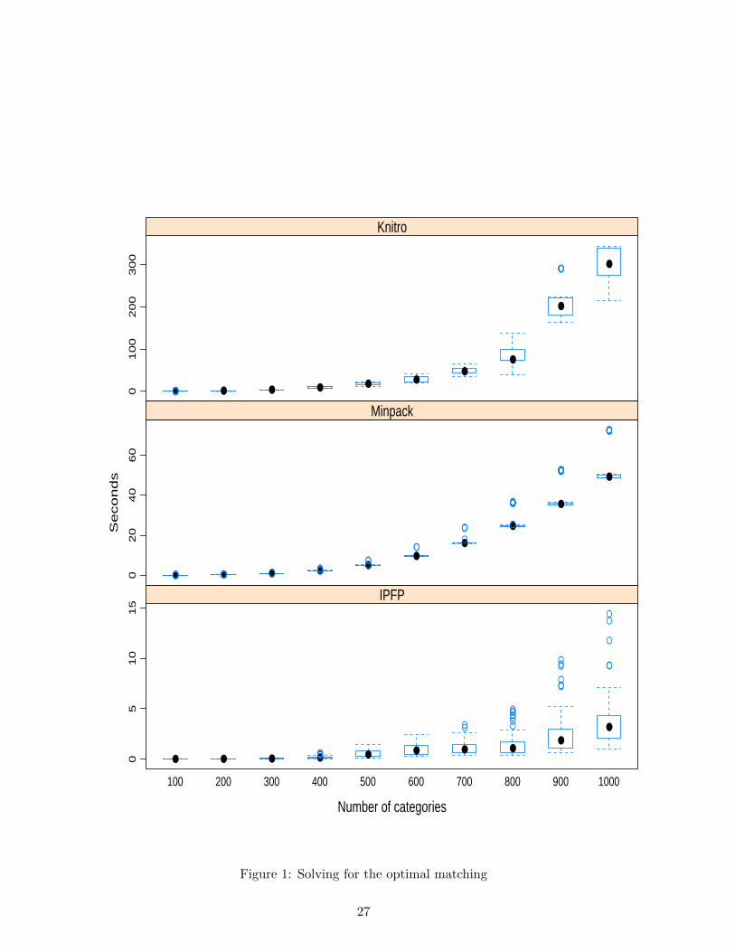
Figure 1. Each panel gives the distribution of CPU times over 50 samples (20 for Knitro)

for the ten experiments, in the form of a Tukey box-and-whiskers graph6.

The performance of IPFP stands out clearly—note the different vertical scales. While

IPFP has more variability than Minpack and Knitro (perhaps because we did not rescale

the problem beforehand), even the slowest convergence times for each problem size are at

least three times smaller than the fastest sample under Minpack, and fifteen times smaller

than the fastest time with Knitro. This is all the more remarkable that we fed the code for

the Jacobian of the system of equations into Minpack, and for both the Jacobian and the

Hessian into Knitro.

6 The Linear Choo and Siow Model

Assume that the analyst has chosen K basis surplus vectors

Φ1xy, ...,Φ

Kxy

which are linearly independent: no linear combination of these vectors is identically equal

to zero.

The analyst then specifies the systematic surplus function Φλxy as a linear combination

of these basis surplus vectors, with unknown weights λ ∈ RK :

Φλxy =

K∑k=1

λkΦkxy (6.1)

6The box goes from the first to the third quartile; the horizontal bar is at the median; the lower (resp.

upper) whisker is at the first (resp. third) quartile minus (resp. plus) 1.5 times the interquartile range, and

the circles plot all points beyond that.

26

Number of categories

Se

co

nd

s

05

10

15

100 200 300 400 500 600 700 800 900 1000

● ● ● ● ● ● ● ●●

●

●●●●●

●●

●●●●●

●●

●

●●●

●●

●

●

●

●

●

IPFP

02

04

06

0

● ● ● ●●

●

●

●

●

●

●●● ●●●● ● ●●●●●●

●●

●

●

●

●●●●

●

●●

●●●●●●●●●●●

●●●●●●●●●●

Minpack

01

00

20

03

00

● ● ● ● ● ●●

●

●

●

●●●●●

●●●●●

Knitro

Figure 1: Solving for the optimal matching

27

where the sign of each λk is unrestricted. We call this specification the “linear Choo and

Siow model” because the surplus depends linearly on the parameters. Quite obviously, if

the set of basis surplus vectors is large enough, this specification covers the full set without

restriction; however, parsimony is often valuable in applications.

To return to the education/income example, we could for instance assume that a match

between man i and woman j creates a surplus that depends on whether partners are matched

on both education and income dimensions. The corresponding specification would have basis

functions like 1(Ei = Ej = e) and 1(Ri = Rj = r), along with “one-sided” basis functions

to account for different probabilities of marrying: 1(Ri = r, Ei = e) and 1(Rj = r, Ej = e).

This specification only has (5nR+2) parameters, while an unrestricted specification7 would

have 4n2R. With more, multi-valued criteria the reduction in dimensionality would be much

larger. It is clear that the relative importance of the λ’s reflects the relative importance

of the criteria. They indicate how large the systematic preference for complementarity of

incomes of partners is relative to the preference for complementarity in educations.

Suppose that the unobserved heterogeneity satisfies Assumption 3. Then the linear

structure underlying model (6.1) makes it very easy to analyze optimal matchings. All

inference can be based on only (K + 1) numbers: the entropy E will be used to test the

specification, and K comoments will be used to estimate λ. Moreover, computing the

Conditional Maximum Likelihood (CML) estimator of λ becomes very easy.

For any feasible matching µ, we define the comoments

Ck(µ) =∑x∈Xy∈Y

µxyΦkxy.

We prove in Appendix A that

Theorem 4 1. The Maximum Likelihood Estimator is characterized by either of the two

equivalent properties:

7Such an unrestricted specification would for instance allow the effect of matching a man in income class

3 with a woman in income class 2 to also depend on both of their education levels.

28

(a) λ maximizes over Λ the concave function

∑x∈Xy∈Y

µxyΦλxy −W (λ) (6.2)

(b) λ solves

Ck(µ) = Ck(µλ) for all k = 1, . . . ,K.

2. Moreover, the entropy of the optimal matching for the CML cannot be smaller than

the entropy of the observed matching:

E (µ) ≤ E(µλ)

and the two entropies are equal if and only if µλ = µ, that is, if and only if the surplus

function in (6.1) rationalizes the observed matching for the CML λ.

Therefore under the assumptions that drive the Choo and Siow model, if the surplus

function is linear in the parameters the Conditional Maximum Likelihood maximizes a very

well-behaved (globally concave) function; and it matches the observed comoments to those

that are predicted by the model. Entropy is a sufficient statistic to test the specification;

and if we cannot reject that the model is well-specified (so that the true data-generating

process is of the form (6.1) for the set of basis functions chosen by the analyst), then the

K comoments form a sufficient statistic to estimate λ.

Our approach to inference has a simple geometric interpretation. Consider the set of

comoments associated to every feasible matching

F =

{(C1, ..., CK

): Ck =

∑xy

µxyΦkxy, µ ∈M (n, m)

}

This is a convex polyhedron, which we call the covariogram; and if the model is well-

specified the covariogram must contain the observed matching µ. For any value of the

parameter vector λ, the optimal matching µλ generates a vector of comoments Cλ that

29

belongs to the covariogram; and it also has an entropy Eλ ≡ E(µλ). We already know that

this model is just-identified from the comoments: the mapping λ −→ Cλ is invertible on the

covariogram. Denote λ(C) its inverse. The corresponding optimal matching has entropy

Er (C) = Eλ(C).

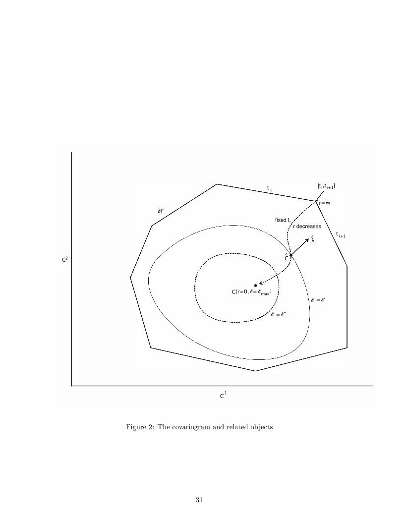
The level sets of Er (.) are the isoentropy curves in the covariogram; they are represented

on Figure 2. The figure assumes K = 2 dimensions; then λ can be represented in polar

coordinates as λ = r exp(it). For r = 0, the model is uninformative and entropy is highest;

the matching is random and generates comoments C0. At the other extreme, the boundary

∂F of the covariogram corresponds to r = ∞. Then there is no unobserved heterogeneity

and generically over t, the comoments generated by λ must belong to a finite set of vertices,

so that λ is only set-identified.

As r decreases for a given t, the corresponding comoments follow a trajectory indicated

by the dashed line on Figure 2, from the boundary ∂F to the point C0. At the same time,

the entropy Eλ increases, and the trajectory crosses contours of higher entropy (E ′ then E ′′

on the figure.) We prove in Appendix A that the CML Estimator λ could also be obtained

by taking the normal to the isoentropy contour that goes through the observed comoments

C, as shown on Figure 2:

Theorem 5 (Geometric identification and estimation) The estimator λ of the pa-

rameter vector is given by the gradient of −Er (.) at the point C.

Concluding Remarks

While the framework we used here is bipartite, one-to-one matching, our results open the

way to possible extensions to other matching problems. Among these, the “roommate

problem” drops the requirement that the two partners of a match are drawn from distinct

populations. Chiappori, Galichon, and Salanie (2012) have shown that this problem is in

30

C

C

∂F

[t

fixed t,

r decreases

1

C2

i,ti+1]

ti+1

ti

(r=0,

r=∞

!=!max)

! =!"

! =!#

C^

λ^

Figure 2: The covariogram and related objects

31

fact isomorphic, in a large population, to an associated bipartite matching problem; as a

consequence, the empirical tools from the present paper can be extended to the study of the

roommate problem. Although an extension to situations of “one-to-many matching” where

one entity on one side of the market (such as a firm) may match with several agents on the

other (such as employees) seems less direct, it is likely that the present approach would be

useful. It may also be insightful in the study of trading on networks, when transfers are

allowed (thus providing an empirical counterpart to Hatfield, Kominers, Nichifor, Ostrovsky,

and Westkamp (2011), Hatfield and Kominers (2012).)

As mentioned earlier, several other approaches to estimating matching models with

heterogeneity exist. One could directly specify the equilibrium utilities of each man and

woman, as Hitsch, Hortacsu, and Ariely (2010) did in a non-transferable utility model.

Under separability, this would amount to choosing a distribution Px and a parameterization

λ of U and fitting the multinomial choice model

maxy∈Y0

(Uxy(λ) + εiy)

to the observed matches of men of type x. The downside is thatunlike the joint surplus, the

utilities U and V are not primitive objects; and it is very difficult to justify a specification

of equilibrium utilities.

An alternative class of approaches pools data from many markets in which the surplus

from a match is assumed to be the same. Fox (2010) starts from the standard monotonicity

property of single-agent choice models, in which under very weak assumptions, the prob-

ability of choosing an alternative increases with its mean utility. By analogy, he posits a

“rank-order property” for matching models with transferable utility: given the character-

istics of the populations of men and women, a given matching is more likely than another

when it produces a higher expected surplus.

Unlike the results we derived from the Choo and Siow (2006) framework, the rank-

order property is not implied by any theoretical model we know of. In our framework, it

holds only when the generalized entropy is a constant function, that is when there is no

matching on unobservable characteristics. The attraction of the identification results based

32

on the rank-order property, on the other hand, is that they extend easily to models with

many-to-one or many-to-many matching.

Finally, Fox and Yang (2012) take an approach that is somewhat dual to ours: while we

use separability to restrict the distribution of unobserved heterogeneity so we can focus on

the surplus over observables, they restrict the latter in order to recover the distribution of

complementarities acroos unobservables. To do this, they rely on pooling data across many

markets; in fact given the very high dimensionality of unobservable shocks, their method,

while very ingenious, has yet to be tested on real data.

33

References

Bajari, P., and J. Fox (2009): “Measuring the Efficiency of an FCC Spectrum Auction,”

University of Michigan mimeo.

Bauschke, H., and J. Borwein (1997): “Legendre Functions and the Method of Random

Bregman Projections,” Journal of Convex Analysis, 4, 27–67.

Becker, G. (1973): “A Theory of Marriage, part I,” Journal of Political Economy, 81,

813–846.

Botticini, M., and A. Siow (2008): “Are there Increasing Returns in Marriage Mar-

kets?,” University of Toronto mimeo.

Byrd, R., J. Nocedal, and R. Waltz (2006): “KNITRO: An Integrated Package for

Nonlinear Optimization,” in Large-Scale Nonlinear Optimization, p. 3559. Springer Ver-

lag.

Chiappori, P.-A., A. Galichon, and B. Salanie (2012): “The Roommate Problem is

More Stable than You Think,” mimeo.

Chiappori, P.-A., R. McCann, and L. Nesheim (2010): “Hedonic Price Equilibria,

Stable Matching, and Optimal Transport: Equivalence, Topology, and Uniqueness,” Eco-

nomic Theory, 42, 317–354.

Chiappori, P.-A., B. Salanie, and Y. Weiss (2012): “Partner Choice and the Marital

College Premium,” mimeo Columbia University.

Choo, E., and A. Siow (2006): “Who Marries Whom and Why,” Journal of Political

Economy, 114, 175–201.

Csiszar, I. (1975): “I-divergence Geometry of Probability Distributions and Minimization

Problems,” Annals of Probability, 3, 146–158.

34

de Palma, A., and K. Kilani (2007): “Invariance of Conditional Maximum Utility,”

Journal of Economic Theory, 132, 137–146.

Decker, C., E. Lieb, R. McCann, and B. Stephens (2012): “Unique Equilibria and

Substitution Effects in a Stochastic Model of the Marriage Market,” forthcoming in the

Journal of Economic Theory.

Fox, J. (2010): “Identification in Matching Games,” Quantitative Economics, 1, 203–254.

(2011): “Estimating Matching Games with Transfers,” mimeo.

Fox, J., and C. Yang (2012): “Unobserved Heterogeneity in Matching Games,” mimeo

University of Michigan.

Gabaix, X., and A. Landier (2008): “Why Has CEO Pay Increased So Much?,” Quarterly

Journal of Economics, 123, 49–100.

Gale, D., and L. Shapley (1962): “College Admissions and the Stability of Marriage,”

American Mathematical Monthly, 69, 9–14.

Galichon, A., and B. Salanie (2010): “Matching with Trade-offs: Revealed Preferences

over Competing Characteristics,” Discussion Paper 7858, CEPR.

Graham, B. (2011): “Econometric Methods for the Analysis of Assignment Problems in the

Presence of Complementarity and Social Spillovers,” in Handbook of Social Economics,

ed. by J. Benhabib, A. Bisin, and M. Jackson. Elsevier.

Gretsky, N., J. Ostroy, and W. Zame (1992): “The nonatomic assignment model,”

Economic Theory, 2(1), 103–127.

(1999): “Perfect competition in the continuous assignment model,” Journal of

Economic Theory, 88, 60–118.

Hatfield, J. W., and S. D. Kominers (2012): “Matching in Networks with Bilateral

Contracts,” American Economic Journal: Microeconomics, 4, 176–208.

35

Hatfield, J. W., S. D. Kominers, A. Nichifor, M. Ostrovsky, and A. Westkamp

(2011): “Stability and competitive equilibrium in trading networks,” mimeo Stanford

GSB.

Hitsch, G., A. Hortacsu, and D. Ariely (2010): “Matching and Sorting in Online

Dating,” American Economic Review, 100, 130–163.

Jacquemet, N., and J.-M. Robin (2011): “Marriage with Labor Supply,” mimeo, Sci-

ences Po.

Shapley, L., and M. Shubik (1972): “The Assignment Game I: The Core,” International

Journal of Game Theory, 1, 111–130.

Shimer, R., and L. Smith (2000): “Assortative matching and Search,” Econometrica, 68,

343–369.

Siow, A. (2009): “Testing Becker’s Theory of Positive Assortative Matching,” Discussion

paper, University of Toronto.

Siow, A., and E. Choo (2006): “Estimating a Marriage Matching Model with Spillover

Effects,” Demography, 43(3), 463–490.

Tervio, M. (2008): “The difference that CEO make: An Assignment Model Approach,”

American Economic Review, 98, 642–668.

36

Appendix

A Proofs

A.1 Proof of Theorem 2

(i) By the classical dual formulation of the matching problem, the market equilibrium assigns

utilities uxi to man i such that xi = x and vyj to woman j such that yj = j so as to solve

W = min

∑i

ui +∑j

vj

where the minimum is taken under the set of constraints

ui + vj ≥ Φxy + εiy + ηxj , ui ≥ ε0i , vj ≥ η0j .

Denote

Uxy = mini:xi=x

{ui − εiy} , x ∈ X , y ∈ Y0

Vxy = minj:yj=y

{vj − ηxj

}, x ∈ X0, y ∈ Y

so that

ui = maxy∈Y0

{Uxiy + εiy} and vj = maxx∈X0

{Vxyj + ηxj

}Then

W = min

∑i

maxy∈Y0

{Uxiy + εiy}+∑j

maxx∈X0

{Vxyj + ηxj

}under the set of constraints

Uxy + Vxy ≥ Φxy , Ux0 ≥ 0 , V0y ≥ 0.

Assign non-negative multipliers µxy, µx0, µ0y to these constraints. By duality in Linear

37

Programming, we can rewrite

W = maxµxy≥0

∑x∈Xy∈Y

µxyΦxy −maxUxy

∑x∈Xy∈Y0

µxyUxy −∑i

maxy∈Y0

{Uxiy + εiy}

−max

Vxy

∑x∈X0y∈Y

µxyVxy −∑j

maxx∈X0

{Vxyj + ηxj

} .

Now,

∑i

maxy∈Y0

{Uxiy + εiy} =∑x

nxEPx maxy∈Y0

{Uxiy + εiy} = nxGx(Ux·),

where EPx denotes the expectation over the population of men in group x, and where we

have invoked Assumption 1 and the law of large numbers in order to replace the sum by an

expectation. Adding the similar expression for women, we get

W = max(µxy)

∑x∈Xy∈Y

µxyΦxy −A (µ)−B (µ)

where

A (µ) = max(Uxy)

∑x∈Xy∈Y0

µxyUxy −∑x∈X

nxGx(Ux·)

B (µ) = max

(Vxy)

∑x∈X0y∈Y

µxyVxy −∑y∈Y

myHy(V·y)

Consider the term with first subscript x in A(µ). It is

∑y∈Y0

µxyUxy − nxGx(Ux·).

It is easy to see that since Gx is the expected maximum utility, for any number t we have

Gx(Ux· + t) = Gx(Ux·) + t; therefore if∑

y∈Y0 µxy 6= nx, the term is plus infinity. This

38

implies that at the maximum in W, the feasibility constraints in (1.2) must hold, and we

can rewrite A(µ) and B(µ) in terms of the rescaled Legendre-Fenchel transforms:

A (µ) =∑x∈X

G∗x (µx·) and B (µ) =∑y∈Y

H∗y(µ·y).

It follows that

W = maxµ∈M(n,m)

∑x∈Xy∈Y

µxyΦxy −∑x∈X

G∗x (µx·)−∑y∈Y

H∗y(µ·y) .

Assigning multipliers ax and by to the feasibility constraints, the first order conditions

of this problem are

Φxy + ax + by =∂G∗x∂µxy

(µx·) +∂H∗y∂µxy

(µ·y)

and

ax =∂G∗x∂µx0

(µx·), by =∂H∗y∂µ0y

(µ·y).

Combining them gives formula (2.8).

(ii) From the proof of part (i), by the envelope theorem

Uxy =∂A

∂µxy(µ);

and since

A (µ) =∑x∈X

G∗x (µx·) ,

adding the normalization Ux0 = 0 gives the formula for Uxy in the theorem.

(iii) By duality, ux = Gx(Ux·) is the multiplier of the feasibility constraint for group x;

and the proof of (i) shows that this is

ax =∂G∗x∂µx0

(µx·).

The proof of (iv) is the same as for (ii) and (iii).

(v) follows from the fact that Uxy = αxy + τxy and Vxy = γxy − τxy; thus if Uxy and Vxy

are identified and τxy is observed, then α and γ are identified by

αxy = Uxy − τxy and γxy = Vxy + τxy.

39

A.2 Proof of Proposition 2

By definition,

Gx(Ux·) = EPx

(maxy∈Y0

(Uxy + εiy)

)and

G∗x(µx·) = maxUx·=(Ux0,...,Ux|Y|)

∑y∈Y0

µxyUxy −

∑y∈Y0

µxy

Gx(Ux·)

.

Now, using the feasibility constraint∑

y∈Y0 µxy = nx :

G∗x(µx·) = −nx minUx·

EPx

(maxy∈Y0

(Uxy + εiy

))−∑y∈Y0

µxynx

Uxy

,

and defining Uxy = −Uxy, this is also

G∗x(µx·) = −nx minUx·

∑y∈Y0

µxynx

Uxy + EPx

(maxy∈Y0

(εiy − Uxy

))The first term in the minimand is the expectation of Ux· under the distribution µY |X=x;

therefore this can be rewritten as

G∗x(µx·) = −nx minUxy+kx(εi·)≥εiy

(EµY |X=x

UxY + EPxkx(εi·))

where the minimum is taken over all pairs of functions (Ux·, kx(εi·) that satisfy the inequal-

ity. We recognize the value of the dual of a matching problem in which the margins are

µY |X=x and Px and the surplus is εiy. By the equivalence of the primal and the dual, this

gives

G∗x(µx·) = −nx maxπ∈Mx

Eπ [εiy] .

A.3 Proof of Theorem 3

The proof uses results in Bauschke and Borwein (1997), which builds on Csiszar (1975).

For any matching µ, consider the function

ϕ(µ) = −E(µ).

40

Since generalized entropy E is concave in µ, ϕ is a convex function. In fact, it satisfies

the conditions in Bauschke and Borwein (1997); in particular it is a Legendre function8.

Introduce D the associated “Bregman divergence” as

D (µ; ν) = ϕ (µ)− ϕ (ν)− 〈∇ϕ (ν) , µ− ν〉 .

Bregman divergences are often called “Bregman distances”; they are not distances, but

they are useful for our purposes because one can generalize the concept of a projection to

Bregman divergences.

Now take any surplus function Φ and margins n amd m. Step 1 of the algorithm

constructs a matching µ(0) such that for all x 6= 0, y 6= 0

Φxy =∂ϕ

∂µxy(µ(0))− ∂ϕ

∂µx0

(µ(0))− ∂ϕ

∂µ0y

(µ(0))

and 2∑

xy µ(0)xy +

∑x µ

(0)x0 +

∑y µ

(0)0y =

∑x nx +

∑y my. Note that while µ(0) adds up to the

total number of men and women, it needn’t satisfy any of the other feasibility constraints.

Moreover, by Theorem 2, the optimal matching for Φ given margins n and m (which always

exists) satisfies all of these constraints; therefore we can always find such a µ(0).

Then⟨∇ϕ(µ(0)), µ− µ(0)

⟩=∑xy

∂ϕ

∂µxy(µ(0))(µxy−µ(0)

xy )+∑x

∂ϕ

∂µx0

(µ(0))(µx0−µ(0)x0 )+

∑y

∂ϕ

∂µ0y

(µ(0))(µ0y−µ(0)0y )

becomes

∑xy

µxyΦxy +∑x

∂ϕ

∂µx0

(µ(0))

(∑y

µxy + µx0

)+∑y

∂ϕ

∂µ0y

(µ(0))

(∑x

µxy + µ0y

),

up to additive terms that depend on µ(0) but not on µ. But if µ ∈M(n, m), then∑

y µxy +

µx0 = nx and∑

x µxy + µ0y = my, so that up to irrelevant terms,⟨∇ϕ(µ(0)), µ− µ(0)

⟩=∑xy

µxyΦxy

8A Legendre function is essentially smooth and essentially strictly convex—see section 2 of Bauschke and

Borwein (1997) for details.

41

and

D(µ, µ(0)) = ϕ(µ) +∑xy

µxyΦxy =∑xy

µxyΦxy − E(µ)

on M(n, m).

Since the optimal matching for surplus Φ and margins n and m maximizes

∑xy

µxyΦxy + E(µ)

it can also be found by minimizing D(µ, µ(0)) over µ ∈M(n, m); that is, by projecting µ(0)

on M(n, m) using the Bregman divergence.

Introduce the linear subspaces M (n) and M (m) by

M (n) =

µ ≥ 0 : ∀x ∈ X ,∑y∈Y

µxy + µx0 = nx

M (m) =

{µ ≥ 0 : ∀y ∈ Y,

∑x∈X

µxy + µ0y = my

}

so that

M(n, m) =M (n) ∩M (m) .

We define µ(k) recursively by iteratively projecting with respect to D on the linear

subspaces M(n) and on M(m):

µ(2k+1) = arg minµ∈M(n)

D(µ;µ(2k)

)(A.1)

µ(2k+2) = arg minµ∈M(m)

D(µ;µ(2k+1)

)(A.2)

By Theorem 8.4 of Bauschke and Borwein (1997), the iterated projection algorithm

converges9 to the projection µ of µ(0) on M(n, m), which is also the maximizer µ of (2.7).

9In the notation of their Theorem 8.4, the hyperplanes (Ci) are M(p) and M(q); and the Breg-

man/Legendre function f is our φ.

42

The updating formulas of the Theorem are easily obtained; let us work out (A.1).

Introduce multipliers ax for the feasibility constraints µ(2k+1) ∈M(n). Neglecting irrelevant

terms again, the Bregman divergence is

D(µ, µ(2k)) = ϕ(µ)−∑xy

∂ϕ

∂µxy(µ(2k))µxy −

∑x

∂ϕ

∂µx0

(µ(2k))µx0 −∑y

∂ϕ

∂µ0y

(µ(2k))µ0y

and the constraints are∑

y µxy + µx0 = nx for all x.

The first order conditions are simply

∂E∂µxy

(µ(2k+1))− ∂E∂µxy

(µ(2k)) = ax for x ∈ X , y ∈ Y0

∂E∂µ0y

(µ(2k+1))− ∂E∂µ0y

(µ(2k)) = 0 for y ∈ Y.

A.4 Proof of Theorem 4

Since W is 1-homogeneous in (n, m, µ),

W =∑x

nx∂W∂nx

+∑y

my∂W∂my

.

Therefore∂W∂λ

=∑x

nx∂2W∂nx∂λ

+∑y

my∂2W∂my∂λ

.

Now by (iii) of Theorem 2,

∂W∂nx

= ux = − logµλx0

nx

hence

∂2W∂nx∂λ

= −∂ logµλx0

∂λ.

Therefore∂W∂λ

= −∑x

nx∂ logµλx0

∂λ−∑y

my

∂ logµλ0y∂λ

. (A.3)

43

Now consider the derivative of the log-likelihood:

∂ logL

∂λ= 2

∑xy

µxy∂ logµλxy∂λ

+∑x

µx0

∂ logµλx0

∂λ+∑y

µ0y

∂ logµλ0y∂λ

.

Since µx0 = nx −∑

y µxy, we get

∑y

µxy∂ logµλxy∂λ

+ µx0

∂ logµλx0

∂λ= nx

∂ logµλx0

∂λ+∑y

µxy

(∂ logµλxy∂λ

− ∂ logµλx0

∂λ

);

adding up with similar terms for women gives

∂ logL

∂λ=∑xy

µxy

(2∂ logµλxy∂λ

− ∂ logµλx0

∂λ−∂ logµλ0y∂λ

)+∑x

nx∂ logµλx0

∂λ+∑y

my

∂ logµλ0y∂λ

;

or, using (A.3),

∂ logL

∂λ=∑xy

µxy

(2∂ logµλxy∂λ

− ∂ logµλx0

∂λ−∂ logµλ0y∂λ

)− ∂W

∂λ.

But given Theorem 1, this is just

∂ logL

∂λ=∑xy

µxy∂Φλ

xy

∂λ− ∂W

∂λ,

which establishes part 1(a) of the Theorem.

Now by the envelope theorem,

∂W∂λ

=∑xy

µλxy∂Φλ

xy

∂λ

since the entropy term does not depend on λ in the Choo and Siow model; this proves part

1(b) since with the linear specification

∂Φλxy

∂λk= Ck(λ).

To prove part 2, note that since µλ maximizes W when λ = λ,

∑x,y

µxyΦλxy + E (µ) ≤

∑x,y

µλxyΦλxy + E

(µλ)

44

and, since E is strictly concave in µ, equality holds if and only if µλ = µ. But

∑x,y

µxyΦλxy =

∑x,y

µλxyΦλxy

by construction, hence

E (µ) ≤ E(µλ)

with equality if and only if µλ = µ.

A.5 Proof of Theorem 5

Let us first prove that

Er(C)

= minλ

(W (λ)−

K∑k=1

λkCk

). (A.4)

Indeed, the optimum is reached at λ = λ(C)

, and there

Er(C)

=W(λ)−

K∑k=1

λkCk = E

(µλ)

which shows (A.4). This implies that Er(C)

is a concave function; and by the envelope

theorem in (A.4), we get∂Er∂Ck

(C)

= λk.

B The Generalized Extreme Values Framework

Consider a family of functions gx : R|Y|+1 → R such that the following four conditions hold:

(i) gx are positive homogeneous of degree one; (ii) they go to +∞ whenever any of their

arguments goes to +∞ (iii) their partial derivatives of order k exist outside of 0 and have

sign (−1)k (iv) and the functions defined by

Px (w0, ..., wJ) = exp(−gx

(e−w0 , ..., e−wJ

))

45

are multivariate cumulative distribution functions. Then introducing utility shocks εx ∼ Px,

we have by a theorem of McFadden (1978):

Gx(w)

nx= EPx

[maxy∈Y0

{wy + εy}]

= log gx (ew) + γ

where γ is the Euler constant γ ' 0.577. Therefore, if∑

y∈Y0 ay = nx, then

G∗x (nx, a) =∑y∈Y0

aywxy (nx, a)− nx

(log gx

(ew

x(nx,a))

+ γ)

where for x ∈ X0, the vector wx (nx, a) solves the system

ay = nx∂

∂wxylog gx

(ew

x), y ∈ Y0. (B.1)

Hence, the part of the expression of E(n,m, µ) arising from the heterogeneity on the

men side is ∑x∈X

nx log gx

(ew

x(nx,µx·))−∑y∈Y0

µxywxy (nx,µx·)

+ C

where C = γ∑

x∈X nx, whose derivative with respect to µxy (x, y ≥ 1) is −wxy (nx,µx·).

C Computations for the Examples

C.1 Computations for Example 1

With type I extreme values iid distributions, the expected utility is

Gx(Ux·) = log∑y∈Y0

exp(Uxy),

and the maximum in the program that defines G∗x(µx·) is achieved in

Uxy = Ux0 + logµxyµx0

.

This yields

G∗x(µx·) =∑y∈Y0

µxy logµxy −

∑y∈Y0

log

∑y∈Y0

which gives equation (3.1). Equation (3.2) obtains by straightforward differentiation.

46

C.2 Computations for Example 2

Consider a man of a group x. Such a man marries a woman of education e′ within social

group g′ with conditional probability

µx,g′e′

µx,g′=

exp(Ux,g′e′/σx,g′)∑Le′=1 exp(Ux,g′e′/σx,g′)

;

and his probability of marrying within group g′ is

µx,g′

nx=

(∑Le′=1 exp(Ux,g′e′/σx,g′)

)σx,g′

1 +∑G

g′′=1

(∑Le′=1 exp(Ux,g′′e′/σx,g′′)

)σx,g′′.

Then, taking logs and subtracting,

Ux,g′e′ = σx,g′ logµx,g′e′

µx,g′+ tx,g′

so that only the constants tx,g′ remain to be determined by solving (with Ux0 = 0 as usual)

µx,g′

nx=

exp(tx,g′)

1 +∑G

g′′=1 exp(tx,g′′).

This gives exp(tx,g′) =µx,g′µx,0

, so that

Ux,g′e′ = logµx,g′

µx,0+ σx,g′ log

µx,g′e′

µx,g′.

The expected utility of this man is

ux = log

1 +

G∑g=1

σx,g′ log

(L∑

e′=1

exp(Ux,g′e′/σx,g′)

)which is

u = log

1 +

G∑g=1

µx,g′

µx,0

L∑e′=1

(µx,g′e′

µx,g′

)σx,g′ .

Finally, the formula for Ux,ge shows that the surplus from a marriage between a man (g, e)

and a woman (g′, e′) is identified by the formula in the text.

47

C.3 Computations for Example 3

We start by giving a formula for G∗x in the slightly more general case where ε is continuously

distributed according to a c.d.f. Fε. From Proposition 2,

G∗x(µx·) = −nx maxπ∈Mx

Eπ [φx (Y ) ε] .

where π has margins Fε and µ(Y |X = x). Since the function (ε, φ) −→ εφ is supermodu-

lar, the optimal matching must exhibit positive assortative matching—larger ε’s must be

matched with y’s with larger values of the index φx(y). Let

φ(1) < . . . < φ(m)

denote the distinct values that the index takes over Y0; value φ(k) has probability

Pr(φx(Y ) = φ(k)|X = x) =

∑φx(y)=φ(k)

µxy

nx. (C.1)

By positive assortative matching, there exists a sequence

ε(0) = inf ε < ε(1) < . . . < ε(m−1)ε(m) = sup ε

such that ε matches with an y with φx(y) = φ(k) if and only if ε ∈ [ε(k−1), ε(k)]; and since

probability is conserved, the sequence is constructed recursively by

Fε(ε(k)

)− Fε

(ε(k−1)

)=

∑φx(y)=φ(k)

µxy

nx. (C.2)

The resulting surplus ism∑k=1

φ(k)E(ε11(ε ∈ [ε(k−1), ε(k)])

).

Now assume that ε is distributed uniformly over [0, 1]. Then (C.2) gives

ε(k) =

∑φx(y)≤φ(k) µxy

nx= Pr

(φx(Y ) ≤ φ(k)|X = x

),

and

E(ε11(ε ∈ [ε(k−1), ε(k)])

)=ε2

(k) − ε2(k−1)

2,

48

which is alsoPr(φx(Y ) ≤ φ(k)|X = x

)−

Pr(φx(Y ) ≤ φ(k)|X = x

)2

Pr(φx(Y ) = φ(k)|X = x

).

Therefore G∗x(µx·) is

−m∑k=1

∑y|φx(y)=φ(k)

φ(k)

Pr(φx(Y ) ≤ φ(k)|X = x

)−

Pr(φx(Y ) ≤ φ(k)|X = x

)2

Pr(φx(Y ) = φ(k)|X = x

);

changing the order of sums and using (C.1) turns this into

G∗x(µx·) = −∑y∈Y0

µxyφx(y)

∑φx(y′)≤φx(y) µxy′ −

∑φx(y′)=φx(y) µxy′/2

nx.

The derivative in µxy has two terms:

−φx(y)

(∑φx(y′)≤φx(y) µxy′ −

∑φx(y′)=φx(y) µxy′/2

nx

)and

−∑y′∈Y0

µxy′φx(y′)1(φx(y) ≤ φx(y′))− 1(φx(y) = φx(y′))/2

nx.

Combining them,

∂G∗x(µx·)

∂µxy= −

∑φx(y′)≤φx(y)

φx(y)µxy′

nx−

∑φx(y)≤φx(y′)

µxy′

nxφx(y′) +

∑φx(y′)=φx(y)

φx(y)µxy′

nx

= −

∑φx(y′)≤φx(y)

φx(y)µxy′

nx+

∑φx(y)<φx(y′)

µxy′

nxφx(y′)

= −E [max (φx (Y ) , φx (y))]

so that

ux = −∂G∗x(µx.)

∂µx0

= E [max (φx (Y ) , φx (0))]

and

Uxy =∂G∗x(µx.)

∂µxy− ∂G∗x(µx.)

∂µx0

= −E [max (φx (Y ) , φx (y))] + E [max (φx (Y ) , φx (0))] .

49