Culture: An Empirical Investigation of Beliefs, Work, and ... · 3 In their famous 1952 book, anthropologists A. L. Kroeber and Clyde Kluckhohn cited 164 definitions of culture. Without

146

American Economic Journal: Macroeconomics 2009, 1:1, 146–177http://www.aeaweb.org/articles.php?doi=10.1257/mac.1.1.146

We observe large variation in economic outcomes across socioeconomic classes, ethnic groups, and countries. What is the role of culture as opposed

to institutions and purely economic factors in explaining the diversity of outcomes? This question, to a very large extent, has been ignored by modern economics. In this paper, we seek to address this lacuna by investigating the contribution of culture to two important economic outcomes: female labor supply and fertility. The focus on these two outcomes that are especially relevant to women is not accidental. Fertility and women’s participation in the formal labor market vary widely across time and space. The hypothesis that a significant portion of this variation can be explained by differences in beliefs and/or preferences regarding the appropriate role of women in society, i.e., by differences in culture, as opposed to economic and institutional

* Fernández: Dept. of Economics, New York University, 19 W. 4th St., New York, NY 10012, and Center for Economic Policy Research (CEPR), National Bureau of Economic Research (NBER), and Institute for the Study of Labor (IZA) (e-mail: [email protected]); Fogli: University of Minnesota, Dept. of Economics, University of Minnesota, 4-173 Hanson Hall, 1925 Fourth Street South, Minneapolis, MN 55455, (e-mail: [email protected]). We thank Oriana Bandiera, Chris Flinn, David Levine, Fabrizio Perri, Jonathan Portes, Frank Vella, Matt Wiswall, and seminar audiences at the Society for Economic Dynamics, NBER, NYU, CERGE at Charles University, University of Cyprus, University of California Berkeley, Stanford University, University of Iowa, Essex University, European University Institute (EUR), Innocenzo Gasparini Institute for Economic Research (IGIER), University of Minnesota, Pompeu Fabra University, The International Society of Logistics (SOLE), European Economic Association, Public Policy CEPR, University of Rochester, Economic Fluctuations and Growth Meeting, Family Conference (Torino), University of Verona, European Summer Symposium in International Economics, Workshop on Culture (Paris), and Conference on Immigration and Culture (Bologna). Fernández thanks the Russell Sage Foundation for its wonderful hospitality. Lastly, we are grateful to Liz Potamites for the excellent research assistance she provided.

† To comment on this article in the online discussion forum visit the articles page at: http://www.aeaweb.org/articles.php?doi=10.1257/mac.1.1.146

Culture: An Empirical Investigation of Beliefs, Work, and Fertility†

By Raquel Fernández and Alessandra Fogli*

We study culture by examining the work and fertility behavior of second-generation American women. Culture is proxied with past female labor force participation and total fertility rates from the woman’s country of ancestry. The values of these variables capture not only economic and institutional conditions but also the country’s preferences and beliefs regarding women’s roles. Since the women live in the United States, only the belief and preference components are potentially relevant. We show that the cultural proxies have posi-tive significant explanatory power even after controlling for educa-tion and spousal characteristics, and we demonstrate that the results are unlikely to be explained by unobserved human capital. JEL: J13, J16, J22, J24, Z13

http://www.aeaweb.org/articles.php?doi=10.1257/mac.1.1.146

VoL. 1 No. 1 147FErNáNdEz ANd FogLi: CULTUrE: WoMEN’S Work ANd FErTiLiTy

variation, seems particularly apt in this context, and the economic importance of these decisions is incontrovertible.

The main challenge of any cultural analysis is how to separate the effects of cul-ture from the effects of strictly economic factors and institutions. The difficulty in achieving this separation has, for the most part, prevented economists from tackling culture.1 One way around this problem is to exploit the difference in the “portabil-ity” of culture relative to economic and institutional conditions. When individuals emigrate, they may take some aspects of their culture with them and transmit them intergenerationally, but they live in the economic and formal institutional environ-ment of the host country. This suggests that studying immigrants or their descen-dents may be a useful strategy for isolating some aspects of culture.2

Before describing our approach, it may be useful to clarify what we mean by “culture.” Culture is a rather hazy concept that lends itself to many alternative defini-tions.3 As defined by the Merriam-Webster Dictionary 2002, culture is (a) “the inte-grated pattern of human knowledge, belief, and behavior that depends upon man’s capacity for learning and transmitting knowledge to succeeding generations”; (b) “the customary beliefs, social forms, and material traits of a racial, religious, or social group.” We will be primarily interested in differences in culture which we define, for our purposes, as systematic differences in preferences and beliefs across either socially or geographically differentiated groups. These preferences/beliefs may be held by the individual and thus influence her actions. They may instead (or also) be held by some portion of the society with whom she interacts (e.g., her family and neighbors). In this case, an individual’s behavior may be influenced as well by the rewards and punishments associated with different actions.

In this paper, we study the work and fertility outcomes of second-generation American women.4 These women, born and raised in the United States, face the same markets and institutions but they potentially differ in their cultural heritage as reflected in their parents’ country of origin. Studying second-generation Americans rather than immigrants has the benefit of minimizing shocks to “normal” behavior resulting from immigration (e.g., language barriers). On the other hand, the fact that they are second-generation Americans is bound to dilute the strength of cultural effects on economic actions since cultural transmission is restricted mostly to par-ents and ethnic social networks rather than operating in society at large (e.g., schools, media, etc.). Thus, from the outset, we consider the power of this test of culture to be asymmetric. Culture may be an important determinant of individual actions within countries but still may not affect immigrants or their descendents if immigrants do

1 Recall George J. Stigler and Gary S. Becker’s (1977) famous indictment of relying, in an ad hoc fashion, on differences in preferences to explain variation in outcomes.

2 We do not mean to suggest that culture, economic factors, and institutions are completely independent of one another. On the contrary, they may well reinforce one another. Our empirical strategy, however, allows us to study how culture operates in isolation from these other factors (though it may not operate with the same effectiveness once it is in a less hospitable environment, i.e., in a different country with a different institutional and economic environment).

3 In their famous 1952 book, anthropologists A. L. Kroeber and Clyde Kluckhohn cited 164 definitions of culture. Without a doubt, many more have been added over the last 50 years.

4 Second-generation Americans are individuals born in the United States whose parents were born elsewhere.

148 AMEriCAN ECoNoMiC JoUrNAL: MACroECoNoMiCS JANUAry 2009

not have preferences and beliefs that are representative of their country’s culture, or if cultural assimilation works rapidly.5

Central to our approach is the use of a quantitative variable as a proxy for culture. In particular, we use past values of female labor force participation (LFP) and total fertility rates (TFR) in the country of ancestry as cultural proxies. The argument for using these variables is as follows. Consider, for example, the variation in female LFP across countries. This aggregate variable reflects the market work decisions of women and hence depends on women’s characteristics and on the economic and institutional environment. A given woman’s decision to work presumably depends on a whole series of economic and institutional factors that may differ across coun-tries such as her wage, her husband’s income (if married), the probability of finding a job, the ability and cost of arranging child care (if she has children), commuting costs, conditions in the marriage market, etc. Her decision will also depend on her preferences and beliefs, broadly defined. That is, it may depend on how she perceives the role of women in the household, her beliefs as to whether children benefit or are harmed by having a working mother, preferences over market and household work, and expectations as to how she would be treated by her local society (e.g., her neigh-bors) as a result of working or not, etc. Hence, female LFP at the aggregate level will depend on the distribution of preferences and beliefs (including beliefs about how others will treat her as a function of her work decision) within a country, and this distribution may also vary across countries, reflecting variation in culture. Now, if this aggregate variable has explanatory power for the variation in work outcomes of second-generation American women, even after controlling for their individual eco-nomic attributes, only the cultural component of this variable can be responsible for this correlation.6 The economic and (formal) institutional conditions of the country of ancestry should no longer be relevant for second-generation American women (as neither the country nor even the time period is the same), whereas the preferences and beliefs embodied in these variables may still matter if parents and/or neighbor-hood transmitted them to the next generation.

The use of a quantitative variable as a proxy for culture is superior to using the woman’s country of ancestry as a proxy variable. The latter suffers from the disad-vantage of not being explicit as to why it may matter to be, for example, of Mexican, as opposed to Swedish, ancestry. Furthermore, the use of a specific quantitative proxy greatly facilitates the task of thinking about possible omitted variables and allows us to test against competing hypotheses directly. We consider this to be an important strength of our approach.

We study the work and fertility outcomes of second-generation American women using the 1970 census, taking the 1950 values of female LFP and TFR in the

5 Recent findings of Francine D. Blau and Lawrence M. Kahn (2007) suggest that some aspects of assimilation may be quick whereas others (e.g., fertility) may take several generations. See George J. Borjas (2007) for a study of the Mexican experience in the United States.

6 It should be noted that we are using “beliefs” in a rather broad sense. An individual’s behavior may depend on expectations (beliefs) of how she will be treated by others. To the extent that immigrants and their descendants cluster in the same neighborhood, they may “recreate” similar social incentives, as in their country of ancestry, although it should be much less costly to move to a different neighborhood and face different expectations. We explore this question further in Section VII.


countries of ancestry as the cultural proxies.7 We find that the cultural proxies are significant in explaining individual work and fertility outcomes. Ceteris paribus, women whose ancestry is from higher female LFP countries work more; women whose ancestry is from higher TFR countries have more children. In order to ensure that these results are not driven by parental characteristics that differ in a system-atic fashion by country of origin (e.g., income or human capital) but that may have economic rather than cultural origins, we control for a woman’s education and the education and income of her spouse.8 We also control for local geographic variation in markets and institutions by including metropolitan standard area fixed effects, and we cluster observations at the country-of-ancestry level. In all cases, we find that culture, as reflected in our proxy variables of LFP or TFR in 1950, is a quantitatively and statistically significant determinant of women’s work and fertility outcomes. A one standard deviation increase in LFP in 1950 is associated with an approximately 7.5 percent increase in hours worked per week in 1970. A one standard deviation increase in TFR in 1950 is associated with approximately 0.4 extra children, a 14 percent increase in the number of children in 1970.

The major concern our analysis needs to address is whether some omitted vari-able exists. The main suspect for this role is unobserved human capital embodied either in the woman or in the “quality” of her ethnic network. Unobserved human capital may be a culprit if differences in parental education levels lead to differences in unobserved human capital in ways not captured by the formal education level of their children. Alternatively, if the human capital of one’s ethnic group is an impor-tant input in the formation of one’s own human capital (as argued by Borjas 1992, 1995), or if it is an input in the ethnic network that helps individuals find employ-ment, then systematic differences in human capital across ethnic groups may be responsible for our results.

We address these concerns in a few ways. We use the General Social Survey (GSS) to control directly for the parents’ level of education and show that our results are robust to these additional controls. As our GSS sample is restricted to a smaller number of countries, we use the 1940 census to calculate the average education of immigrants by country of origin. This variable should proxy for parental human capital and for the human capital embodied in the ethnic network available to the woman. We find that the effect of the cultural proxy remains robust. We also con-struct a similar measure of ethnic human capital for second-generation immigrants to obtain similar results. It is also possible that it is the quality, rather than quantity, of human capital that matters. We use education quality data by Eric A. Hanushek and Dennis D. Kimko (2000) based on performance on international standardized tests to investigate this issue and find that our cultural proxies remain significant. Lastly, we examine wages directly. If the significance of our cultural proxy is being driven by unobserved human capital, then the latter should help explain variation in the wage rate. We run standard Mincer regressions with and without selection and show that our cultural proxy does not help predict women’s wages.

7 Later decades of the census do not ask for the country of birth of a respondent’s parents, and 1950 is as far back as one can go to obtain female LFP and TFR for a nontrivial number of countries.

8 Our dataset does not permit us to observe the financial and educational backgrounds of parents directly.


A married woman’s decision is also likely to depend on her husband’s prefer-ences. Whose culture is important in deciding a married woman’s work and fertility, her own or her husband’s? We show that the cultural proxies of both spouses play an important role, though perhaps surprisingly, the husband’s culture appears to be, if anything, more important in driving his wife’s work outcomes.9

Lastly, we show that there appears to be a social component to the behavior we study. In particular, we show that the impact of the cultural proxies is larger for those ancestries that show a greater tendency to cluster in the same neighborhoods. This could result from a stronger transmission of preferences and beliefs in an envi-ronment that presumably bears greater resemblance to the parents’ original social environment (e.g., from a larger number of role models), or it could result from the greater importance of the social rewards/punishments associated with different behavior when women live in neighborhoods with a larger percentage of individuals from their country of ancestry.

Our paper is organized as follows. Section I contains a brief review of the empiri-cal literature. Section II presents our empirical strategy, and Section III presents our results. Section IV examines whether unobserved human capital may be responsible for our results. Section V investigates whether it is a woman’s or her husband’s cul-ture that matters for her outcomes, and Section VI studies the role of ethnic density in the neighborhood. Section VII concludes.

I. A Brief Literature Review

The idea that culture can influence economic outcomes is, of course, not a new one. Max Weber’s celebrated thesis at the beginning of the twentieth century argued that a specific culture, the “Protestant ethic,” was conducive to capitalist accumula-tion. More recently, culture played a central role in David S. Landes’ (1998) explana-tion for differences in economic growth across countries. Robert D. Putnam (2000) stresses the role of trust, and more generally of “social capital,” in facilitating eco-nomic exchange and efficient governance.10

There is little quantitative evidence, however, that demonstrates culture is a sig-nificant determinant of important economic outcomes. In fact, probably the best-known paper in this field (Christopher D. Carroll, Byung-Kun Rhee, and Changyong Rhee 1994) finds that culture does not help explain differences in saving rates. The authors study immigrants in Canada using a household data set which allows them to identify immigrants by region, though not by country of origin. They find that, although there is an immigration effect common to the savings behavior of those who were not born in Canada, there is no effect of culture that further distinguishes

9 This evidence is also in line with Fernández, Fogli, and Claudia Olivetti (2004). They show that a quan-titatively important factor explaining whether a man’s wife works is whether his own mother worked when he was growing up. This finding holds even after controlling for education, income, and other family background variables. Whether his mother worked or not is probably influenced by her beliefs about women’s roles, which may then have been transmitted to her son and influenced any household bargaining/decision affecting his wife’s work outcome.

10 See David N. Weil’s (2004) very nice chapter that reviews the research on culture and growth. See Maristella Botticini and Zvi Eckstein (2005) for a historical account of how “exogenous” changes in Jewish culture gave rise to human capital accumulation and, subsequently, occupational selection.


the savings behavior of immigrants from different regions. As the authors acknowl-edge, however, their conclusions must be viewed as tentative due to data restrictions. In particular, they can control only for broad regions of origin, wealth is imperfectly measured, and remittances are not observed.

Our paper belongs to a very recent literature that has attempted to meet the chal-lenge of showing, in a quantitative fashion, that culture matters.11 Recent papers by Robert J. Barro and Rachel McCleary (2003) and Guido Tabellini (2005) study the impact of culture on growth. Barro and McCleary show that the degree of reli-giosity of a country is significant in explaining differences in growth rates across countries. Tabellini studies growth across regions of Europe and shows that regional variation in answers to questions about trust, respect for others, and how confident one is about the link between individual effort and economic success helps explain growth. To tackle the issue of causality, he instruments the answers with histori-cal variables such as past values of regional literacy rates and political institutions and shows that these variables help explain differences in per capita growth rates. Luigi Guiso, Paola Sapienza, and Luigi Zingales (2004) present evidence that cul-ture affects trust and trade.12 They use commonality of religion, the genetic distance between indigenous populations, and the history of wars between nations as prox-ies for culture, and show that these are correlated with a measure of trust. Trust is then shown to be quantitatively significant in explaining the amount of economic exchange between countries. There is also some evidence that culture affects living arrangements and labor market outcomes. Paola Giuliano (2005) shows that children of Western European immigrants to the United States replicate the family living arrangements of their country of origin. Yann Algan and Pierre Cahuc (2005) show that cultural attitudes toward the family affect the employment patterns of different demographic groups in Organisation for Economic Co-operation and Development (OECD) countries, whereas Algan and Cahuc (2006) provide evidence that civic culture affects the design of labor market institutions such as employment protection and unemployment benefits.

There has also been some work in the fields of labor and fertility that examines the interrelationship between country of origin and economic outcomes.13 Using ethnic dummy variables, Cordelia W. Reimers (1985) is an early attempt to exam-ine the role of ethnicity in married women’s labor force participation in the United States. She finds mixed evidence in favor of ethnic background mattering, which, perhaps, is not surprising given that ethnic groups vary substantially in the length of time they have been in the United States. Heather Antecol (2000) uses a similar strategy to study the effect of male and female LFP in the country of ancestry on the inter-ethnic gender gap in labor force participation rates in the United States. She

11 There is, of course, an immense sociological and anthropological literature that studies the impact of cul-ture on a variety of outcomes which we do not attempt to review here. To our knowledge, however, this literature has not been quantitative.

12 See Avner Greif (1994) for a historically based account of why culture may matter to trade.13 It has already been noted that if one assumes unchanged preferences, wages from the mid-1970s to the

mid-1990s, for example, can at most account for half of the observed change in work behavior across cohorts in the United States (see John Pencavel 1998). Fernández, Fogli, and Olivetti (2004) present a model of endogenous preference evolution through family experience and explore the role of these preferences in increasing female labor force participation.


studies first- generation immigrants and groups together second and higher genera-tion individuals. The results are suggestive that ethnicity matters but they leave open the possibility that they could be driven by other factors that differ across countries such as education levels, or from differences in parental background that lead to systematic variations in unobserved human capital. These alternative hypotheses are not examined.

There is also a literature that studies the effect of culture on fertility.14 This includes, for example, Timothy W. Guinnane, Carolyn M. Moehling, and Cormac Ó Grada (2006) who study Irish fertility in the United States in 1910, and Blau (1992) who examines the fertility behavior of first-generation immigrant women in the United States.15 These investigations, however, face difficult issues such as selection into immigration and the possible disrupted and delayed fertility behavior that may result from immigration. By examining second-generation women in the United States, our analysis mitigates these concerns.

In addition to the above studies focusing on immigrants, there has been work using measures of attitudes toward women’s roles within a country. David I. Levine (1993), for example, finds that attitudes, as reflected in responses to GSS questions, are an important predictor of whether any particular woman works in a given year, but that attitudes are not able to explain the increase in women’s labor force partici-pation during the 1970s and early 1980s. Francis Vella (1994) uses Australian data and likewise finds that attitude variables are important determinants of the extent of women’s involvement in market work. A more recent paper, written by Nicole M. Fortin (2005), uses the World Value Surveys to show that gender role and work attitudes help explain work and fertility outcomes for 25 OECD countries.

II. The Empirical Strategy, Datasets, and Sample Selection

As discussed in the introduction, our empirical strategy is to isolate the effects of culture from those of markets and institutions by studying the work and fertility outcomes of women who were born in, and reside in, the United States, but whose parents were born in another country. We use past aggregate outcomes in the wom-an’s country of ancestry to proxy for culture, as only this component of the variable should have explanatory power in a new environment. The issue of a potential omit-ted variable is discussed in Section IV.

Our main dataset is the 1 percent 1970 Form 2 Metro Sample of the US Census. We use the 1970 census since this is the last year in which individuals were explic-itly asked where their parents were born.16 The 1970 census does not provide the

14 See Robert A. Pollack and Susan Cotts Watkins (1993) for an interesting review of various approaches to fertility.

15 Guinnane, Moehling, and Ó Grada (2006) find that, although Irish fertility fell in the United States rela-tive to couples in Ireland, Irish immigrants still had larger families than the native-born population in the United States (conditional on differences in other observable population characteristics). Blau finds that the home country variable (TFR) enters positively and significantly into explaining the fertility behavior of immigrant women in 1970 and 1980. See also Jon Gjerde and Anne McCants (1995) for an analysis of how culture affected the marital and fertility decisions of Norwegian immigrants to the United States.

16 In subsequent decades, individuals were asked to declare their “ancestry,” and thus it is impossible to dis-tinguish between individuals whose families have been in the United States for many generations from those that


country of birth of an individual’s mother when both parents were born outside the United States. Hence, we use the father’s birthplace to assign a country-of-ancestry culture to the second-generation women in our sample.

Our main sample consists of married women who are 30–40 years old. Women in this age range have completed their education but are still far from retirement con-siderations. We focus on married women as they display the largest variation in work and fertility outcomes.17 We exclude women living in farms or working in agricul-tural occupations, as well as those living in group quarters (e.g., prisons, and other group living arrangements such as rooming houses and military barracks).18 There are 87,305 women who are born in the United States and satisfy these criteria.19 About 11 percent of them have fathers who were born outside the United States and are thus included in our sample. From this group, we eliminate those who respond to the question about their father’s birthplace with a continent or a geographical area from which a country cannot be identified.

To study women’s labor outcomes, we mainly use the number of hours worked in the previous week (all the other specifications, instead, go through using the number of weeks worked in the year). This information is reported in intervals.20 We com-pute our measure of time worked by assigning the midpoint of each chosen interval. The census also asks women to record the number of children born to them. We use the response to this question to study fertility.

We use past values of female LFP and TFR for the country of ancestry as our cul-tural proxies. As discussed in the introduction, these variables reflect the economic, institutional, and cultural effects on women’s decisions but only the cultural com-ponent can potentially have explanatory power for the work and fertility outcomes of women born and raised in a country with a different economic and institutional environment. The optimal decade from which to take these numbers is not obvi-ous. As the women in our sample are 30–40 years old in 1970 and were born in the United States, their parents must have come to the United States by 1930–1940, depending on the precise age of the woman. Thus, on the one hand, it could be argued that the values of the culture proxy variables from 1930–1940, or even a decade or two earlier, would best reflect the culture of the country of ancestry. On the other hand, one could argue that the values that parents and society transmit are best reflected in what the counterparts of these women are doing in the country of ancestry in 1970. Data limitations, in any case, do not permit us to use years prior to 1950 since values for neither variable are available for more than a handful of countries prior to that year. Consequently, we choose female LFP and TFR in 1950

are second-generation Americans. Using earlier decades presents the problem that we cannot obtain female LFP and TFR for more than a handful of countries prior to 1950.

17 Our robustness section shows that our results are valid for all women regardless of marital status.18 We exclude the following occupations based on the 1950 census definition: farmers (owners and tenants),

farm managers, farm foremen, farm laborers as wage workers, farm laborers as unpaid family workers, and farm service laborers as self-employed.

19 We exclude from the sample women born in the US outlying areas and territories (American Samoa, Guam, Puerto Rico, US Virgin Islands, and other US possessions). We also exclude from the sample women who were born in the United States but in an unidentified state. Their inclusion does not alter the results.

20 The number of hours worked in the previous week are recorded in 8 intervals: 1–14 hours, 15–29 hours, 30–34 hours, 35–39 hours, 40–48 hours, 49–59 hours, and 60+ hours. All other observations are coded as N/A and treated as zeros in this work.


in the country of ancestry as our benchmark cultural proxies, but explore 1960 and 1970 values as well.

The cross-country data for 1950 female LFP and TFR are from the International Labor Organization (ILO) and the United Nations demographic yearbook, respec-tively. Female LFP is the rate of the economically active population for women over 10 years of age.21 The TFR is the average number of children a hypothetical cohort of women, from the ages of 15 to 49, would have at the end of their reproductive period if they were subject during their whole lives to the fertility rates of a given period, and if they were not subject to mortality. It is expressed as number of chil-dren per woman.

We conclude our selection by eliminating from our sample all women whose fathers were born in countries that became centrally planned economies around World War II.22 The rationale for doing this is that the parents of our women must have been in the United States by 1940. Hence, the parents did not live through the profound transformations in the economies, institutions, and cultures that these countries experienced over that period, and using data from the 1950s and later would not capture the correct culture for these individuals. We also excluded Russia, since the revolution was in 1917 and the parents may or may not have been there for any substantial length of time thereafter. For robustness, we have also run our regres-sions with Russia and our results are unaffected. Last, solely in order to be able to make meaningful comparisons across averages of women by country of ancestry, we also eliminated those countries with fewer than 15 observations.23 Since our regres-sions are all run at the individual level, including these small numbers of observa-tions does not affect our results. Our final sample consists of 6,774 women and 25 countries of ancestry.24

In Table 1, we report the summary statistics at the country level. Our countries are mainly European (17 countries), with a few countries in the Americas (Canada, Cuba, and Mexico), some in Asia (China, Japan, and the Philippines), and some in the Middle East (Syria and Lebanon). Female LFP in 1950 is, on average, 24.4 with a standard deviation of 11.4. It varies dramatically by country, from 7 percent in Lebanon to over 50 percent in Turkey. The TFR in 1950 also shows large variation, from 6.9 children in Turkey and Mexico to 2.1 in Austria. The average across coun-tries is 3.7 with a standard deviation of 1.8. Interestingly, the cross-country correla-tion of female LFP and TFR in 1950 is practically zero (0.002).

The women in our sample are, on average, 35.7 years old, have 3.1 children, and worked, on average, 10.2 hours in the previous week. There is large dispersion in the number of hours worked and number of children, 16.3 hours and 1.8 children, respectively. Comparing the women in our sample with their counterparts whose

21 The active population includes persons in “paid” or “unpaid” employment, members of the armed forces (including temporary members), and the unemployed (including first-time job seekers). “Unpaid” employment includes employers, own-account workers and members of producers’ cooperatives, unpaid family workers, per-sons engaged in the production of economic goods and services for own and household consumption, and appren-tices who receive pay.

22 We eliminated Albania, Bulgaria, Czechoslovakia, Estonia, Hungary, Latvia, Lithuania, Poland, Romania, and Yugoslavia.

23 Iceland, Luxemburg, Korea, India, Iran, and Jordan.24 Note that we do not impose any restrictions on the characteristics of these women’s husbands.


fathers were born in the United States, the latter have a similar number of children on average (3.0). Women with fathers born in the United States, on average, worked more and had a higher standard deviation, 13.1 hours a week and 18.0 hours, respec-tively. The summary statistics are reported in Table A1 in the Appendix.

The differences across work and fertility in 1970 for the women in our sample can also be seen when we group observations by country of ancestry, as was done in Table 1. Women with Cuban fathers worked 15.2 hours on average, while women with Syrian fathers worked 5.1 hours on average. Women with Mexican fathers, on average, have 4.2 children, whereas women with Turkish fathers have 2.2 children. The standard deviation in work and fertility by country of ancestry (2.6 for hours worked and 0.4 for children) is considerably smaller than the standard deviation in these variables across all women. It is also smaller than the standard deviation by country of ancestry in the levels of 1950 LFP and TFR. The correlation between hours worked in 1970 and female LFP in 1950 is 0.25, whereas the correlation between children and TFR 1950 is 0.13.

One may object from the outset that there is no reason to believe immigrants have the preferences/beliefs that are representative of the average in their country of origin. This may or may not be true for different cultural attributes, but in any case this factor will tend to bias the test of our hypothesis toward not finding any

Table 1—Country Summary Statistics

Hours Female LFP TFR H. Cap. H. Cap. Avg. ethnicCountry Observations worked Children 1950 1950 1940 1970 density

Canada 720 10.41 3.29 17.82 3.73 9.60 12.10 7.40Mexico 839 10.87 4.22 8.42 6.87 4.59 9.17 18.10Cuba 17 15.24 2.41 12.19 4.10 8.13 12.50 4.70Denmark 80 12.20 3.00 32.32 2.54 9.45 12.63 0.90Finland 54 11.07 2.56 39.56 2.97 7.43 12.44 3.90Norway 141 10.49 2.82 20.11 2.60 9.00 12.44 3.00Sweden 187 9.93 2.74 23.21 2.21 8.89 12.77 1.70United Kingdom 498 9.43 2.86 25.34 2.18 9.77 12.86 1.20Ireland 465 7.42 3.51 22.95 3.38 8.33 12.70 3.30Belgium 24 6.58 3.29 18.98 2.33 8.52 12.08 0.70France 66 9.74 3.14 28.28 2.73 9.29 12.31 0.30Netherlands 101 9.55 3.16 18.65 3.06 8.85 12.29 3.90Switzerland 50 12.78 3.24 25.73 2.28 9.60 12.62 0.80Greece 197 9.47 2.48 17.95 2.29 7.07 12.83 1.10Italy 1,909 9.77 2.76 20.99 2.32 5.91 11.76 12.10Portugal 100 11.83 3.13 16.99 3.04 5.15 10.74 6.80Spain 65 8.71 2.58 12.56 2.57 6.84 12.22 —Austria 270 9.96 2.77 36.29 2.09 7.64 12.58 2.10Germany 616 10.82 2.87 34.23 2.16 8.95 12.48 3.20China 53 13.27 2.64 47.12 6.22 7.30 13.52 6.20Japan 148 16.84 2.43 32.99 2.75 9.36 13.03 12.60Philippines 67 14.53 3.07 23.75 7.29 9.08 11.72 6.50Lebanon 27 10.50 3.04 6.90 5.74 1.50 12.73 0.40Syria 38 5.09 2.82 14.85 7.20 6.97 12.35 0.80Turkey 42 10.63 2.21 52.76 6.90 7.58 13.44 0.30

Average 270.96 10.68 2.92 24.44 3.66 7.79 12.33 4.25Standard deviation 414.12 2.57 0.42 11.40 1.83 1.92 0.86 4.54

Sources: 1 percent 1970 Form 2 Metro Sample of the US Census, 1 percent 1940 General Sample of the US Census, ILO, Economically Active Population, 1950–2010, (Geneva, 1997), United Nations demographic yearbook 1997, Historical supple-ment table 4, Borjas (1995), table 2, Borjas (1995). For variable definitions, see text.


effect of culture on work and fertility. More importantly, it is difficult to think of a plausible story whereby selection into immigration should bias the results in favor of culture. If all countries share the same culture (or if culture does not matter), a selec-tion story would require immigrants from high female LFP (high TFR) countries to possess higher-than-average preferences/beliefs towards work (ideal family size) and immigrants from low female LFP (low TFR) countries to possess lower-than-average preferences and beliefs. There is no reason to expect this to be the case.

For our analysis to be meaningful, culture should evolve relatively slowly over the time period in which we are interested. Otherwise, in general, the beliefs transmit-ted from parents to children would not be captured by past values of female LFP and TFR. Although we cannot examine the values for our cultural proxies 20 years earlier to verify this, we can look at them 20 years later, i.e., in 1970. We find very high correlations over time for both variables.25

III. Results

We estimate the following model:

(1) zisj = β0 + β′1 Xi + β2 z̃j + fs + εisj,

where zisj is the work/fertility decision of woman i who resides in the Standard Metropolitan Statistical Area (SMSA) s and is of ancestry j.26 In Xi, we include a set of individual characteristics which varies with the specification considered, fs is a full set of dummies for the metropolitan area of residence, and z̃j is the proxy for cul-ture (our variable of interest) which is assigned by the country of father’s birthplace. Since the key variable on the right-hand side only varies by country of ancestry, all the standard errors we report are corrected for clustering at the country-of-ancestry level.

Table 2 presents our main results. In column 1, the amount worked by individual i is regressed on the cultural proxy for work, female LFP in 1950 assigned by coun-try of ancestry, and on a full set of dummies for the woman’s metropolitan area of residence. The coefficient on the cultural variable is positive and strongly significant, indicating that women whose parents were born in countries where women partici-pated less in the work force tend to work less themselves.

There may be many reasons for the positive partial correlation above that have little to do with culture. In particular, parents may differ in a systematic fashion by country of origin in a way that affects their daughters’ propensity to work. For example, if higher levels of education increase the incentives to work, and if it is less costly for a woman to become educated if her parents come from a high female LFP

25 The rank (Spearman) correlation across countries for female LFP in 1950 and 1970 is 0.93. The rank cor-relation for those same two decades in TFR is 0.85. The Pearson and rank correlations for our set of 25 countries during the period of 1950–2000 is 0.51 and 0.50, respectively. Over time, TFR has decreased in all countries. The Pearson and rank correlations in TFR from 1950 to 1995 remain remarkably high: 0.86 and 0.70, respectively.

26 An SMSA is an area consisting of a large population center and adjacent communities (usually counties) that have a high degree of economic and social interaction with that center. A total of 117 SMSAs (including not residing in an SMSA) are identified in the data.


country (e.g., because these parents are, themselves, more educated, or because they have higher income or wealth), then this correlation would be due to the correlation between parental characteristics by country of origin and female education. This would suggest that, given that information on parental characteristics is unavailable, we may want to control directly for a woman’s level of education. By doing so, how-ever, we do not capture the indirect effect of culture on a woman’s desired level of education (i.e., if higher female LFP is associated with a greater willingness to work, this may lead women to acquire higher levels of education as the latter increases the return to market work), but only the direct effect of culture on work.

The regression results from including a series of individual characteristics, in particular the woman’s age (and its square) and a set of dummy variables to cap-ture her level of education (below high school, omitted; high school degree, High school; some college; and at least a college degree, College +), are reported in the second column. As expected, women with more education tend to work more. The direct effect of culture remains positive and statistically significant, albeit somewhat smaller in magnitude, indicating that a woman’s education and female LFP in her country of ancestry tend to be positively correlated.

Table 2—Culture, Work, and Fertility

Dependent variable is hours worked Dependent variable is children

(1) (2) (3) (4) (5) (6) (7) (8) (9)

Female 0.047*** 0.041** 0.072*** 0.045*** 0.053*** −0.010 LFP 1950 (0.012) (0.016) (0.015) (0.014) (0.016) (0.008)

TFR 1950 −0.225** 0.250*** 0.219*** 0.219*** 0.194***(0.103) (0.056) (0.041) (0.041) (0.051)

High school 0.490 2.136*** 2.114*** 2.059*** −0.415** −0.393*** −0.378**(0.520) (0.575) (0.511) (0.572) (0.181) (0.151) (0.147)

Some college −0.147 3.205*** 3.336*** 3.160*** −0.503** −0.485*** −0.457**(1.078) (1.034) (0.963) (1.024) (0.213) (0.185) (0.179)

College + 0.815* 6.032*** 6.744*** 5.968*** −0.869*** −0.865*** −0.838***(0.492) (0.494) (0.448) (0.480) (0.214) (0.204) (0.195)

Husband −1.737** −1.826*** −1.789** −0.218* −0.210* high school (0.730) (0.694) (0.716) (0.116) (0.113)

Husband −1.329 −1.312* −1.370* −0.184* −0.177* some college (0.829) (0.786) (0.822) (0.103) (0.103)

Husband −5.003*** −4.467*** −5.054*** −0.194*** −0.185*** college + (0.452) (0.493) (0.459) (0.050) (0.049)

Husband −2.844*** −2.806*** −2.862*** 0.116** 0.118** total income (0.308) (0.258) (0.303) (0.049) (0.049)

Child < 5 −7.536***(0.554)

Observations 6,774 6,774 6,774 6,774 6,774 6,774 6,774 6,774 6,774Adjusted r2 0.018 0.024 0.053 0.053 0.098 0.059 0.098 0.105 0.106

Notes: SMSA fixed effects in all specifications. Age and age squared for wife and age range dummies for husband in all specifi-cations with demographics. Robust standard errors in parentheses account for clustering at country level. Income is measured in units of $10,000. All specifications include a constant. *** Significant at the 1 percent level. ** Significant at the 5 percent level. * Significant at the 10 percent level.


It may also be important to include the characteristics of a woman’s husband in our regression analysis. These characteristics can be influenced by unobserved parental characteristics, by assortative matching in marriage, or by cultural consid-erations. If a woman wishes to engage in market work, for example, this may lead her to choose a husband with characteristics that support this choice. If a woman prefers to work at home, this may lead her to place more emphasis on characteristics such as her husband’s income.27 These would be the indirect effects of culture on marriage. On the other hand, the forces of assortative matching may swamp any cultural considerations. If there is assortative matching in education (say as a result of considerations about the “quality” of children), then more educated (and hence higher income) men would tend to be married to more educated women (as indeed they are). Thus, on average, women from higher female LFP countries would tend to be married to men with higher education and higher income. The husband’s higher income will decrease the incentives for his wife to engage in the work market and, in this way, will also mask the strength of the different preferences/beliefs held by women from higher female LFP countries vis-á-vis work. The third column explores this question by including the following characteristics of a woman’s husband: his age (as given by ten different age-range dummies), his education (as captured by the same four dummy variables as for the woman), and his total income.28 We will, henceforth, refer to the regression in which the characteristics of both the wife and the husband are included as the “full specification.”

As shown, a husband’s characteristics are important determinants of a woman’s labor supply. A woman whose husband has at least a college degree, everything else equal, works, on average, five hours less per week than a woman whose husband did not complete high school—almost half the mean labor supply of the women in our sample. Marriage to a man with $10,000 more income over the mean is associ-ated, on average, with a woman working almost 3 hours less a week. The effect of culture remains positive and statistically significant at the 1 percent level, with the coefficient increasing significantly in magnitude (as do the coefficients on female education). The latter indicates that there is a positive correlation between a woman’s education and her husband’s education and total income, as well as between these characteristics and female LFP in her country of origin. When we do not control for the husband’s characteristics, the woman’s education picks up the positive effect of her cultural heritage and the negative effect of her husband’s income and education, lowering the coefficient on her own education. Similarly, when we omit the husband’s characteristics, the culture proxy also picks up the negative effect of women from higher LFP countries tending to marry men with higher education and income.

In the full specification, an increase in the level of female LFP in 1950 by one standard deviation (across countries) is associated with an increase of 0.82 hours worked per week, which is about 30 percent of the variation in hours worked per week across ancestries.

27 See Fernández, Nezih Guner, and John Knowles (2005) for an analysis of the potential trade-offs between love and money in household formation.

28 Income is given by the total pretax personal income from all sources for the previous calendar year and is measured in tens of thousands of dollars.


Some analyses of labor supply include the number of children as an explanatory variable. As we are primarily interested in investigating the effect of culture, and work and fertility are simultaneously determined variables both affected by culture, we do not include the number of children in the labor supply equation. We have, nonetheless, included a specification in which we control for the presence of a child under the age of five living in the household (Child5), as this affects the tendency to work but does not fully capture the impact of culture on family size. As shown in column 4 of Table 2, our cultural proxy remains significant at the 1 percent level.29

Our analysis of women’s fertility behavior in Table 2 repeats the same regression strategy used to analyze work, as shown in columns 6–8. For all our specifications, the culture proxy, the TFR in 1950 in the country of ancestry, is positive and statis-tically significant. Unlike for our work results, however, the magnitudes on all the variables remain more or less constant through the different exercises. Higher levels of education, both a wife’s and her husband’s, are associated with fewer children, whereas higher total income is associated with higher fertility. Having a husband who makes $10,000 more over the mean increases the number of children by 0.12.

In the full specification, an increase of one standard deviation in 1950 TFR is associated with an increase of 0.40 children, which represents over 95 percent of the standard deviation of number of children across ancestry. It appears, therefore, that cultural differences across countries may explain a large part of the variation across ethnic groups.

Our two culture proxies may have independent power to explain work and fertil-ity, as these two variables may capture different aspects of culture. For example, both variables may reflect, in part, the belief as to the appropriate role of women in society, but 1950 TFR may also capture some independent cultural preferences for family size (recall that the correlation of these two variables across countries, surprisingly, is basically zero). Thus, in columns 5 and 9, we examine the effect of including both cultural proxies in our work and fertility regressions, respectively. The effect of including both proxy variables is asymmetric across work and fer-tility. TFR in 1950 has explanatory power in the work regression (negative), but female LFP in 1950 does not help explain fertility. An increase in TFR 1950 by one standard deviation is associated with a 0.71 decrease in weeks worked and a 0.41 decrease in hours.

The results above show that a woman’s cultural heritage is an important factor in determining her work and fertility decisions. As shown in our working paper (Fernández and Fogli 2005), the results are robust to changes in sample criteria, alternative estimation techniques, and alternative variables as cultural proxies. In particular, we included all women independently of their marital status (and used marital status dummies), included Russia or excluded China (as arguments could be made for either), and independently excluded Mexico and Italy as these countries have particularly large samples. We also ran an ordered Probit with the nine pos-sible hour interval outcomes and a Tobit regression for hours worked (as our sample contains a large number of women who do not work but may be very heterogeneous).

29 We also ran a seemingly unrelated regression for work and fertility.


We also examined the participation decision itself. For alternative cultural prox-ies, we used the percentage of the workforce that is female in 1960 and the labor force participation of women 30–34 years old in 1950. To ensure that the results are not driven by the disruptions associated with World War II (WWII), we also used 1960 female LFP and TFR. Lastly, we examined the effect of the cultural proxy on completed fertility by changing the sample age of women to 40–50 years old. In all cases, our results were robust to these alternative specifications.

A. Country dummies and Cultural Proxies

Next, we turn to the more traditional approach of estimating (1) by using country dummies rather than the quantitative home country variables as our cultural proxies. This has the benefit of not requiring the relationship between culture and outcomes to be linear in the cultural proxy. Furthermore, it may allow different features of cul-ture to play a role in work and fertility outcomes other than those captured in 1950 LFP and TFR. It has the previously discussed drawback, however, of not specifying how culture matters.

Panel A of Table 3 reports the coefficients obtained on each country dummy from running the full specification of (1) for hours worked and number of children. For the work regressions, the omitted country is Mexico which has the lowest value of female LFP in 1950 in the sample. For fertility, the omitted country is the one with the lowest TFR in 1950, Austria. Since we are now estimating the same number of parameters as the number of countries of ancestry in the sample, we restrict the sample to countries for which we have at least 50 observations, leaving us with 6,626 observations and 20 countries.30

In our work and fertility regressions, the country dummies are jointly, highly significant. The magnitude of the country-of-ancestry effect ranges from four addi-tional hours worked per year by women with Japanese ancestry to essentially zero for women with Irish ancestry, as compared to their Mexican counterparts. For fer-tility, the country-of-ancestry effect ranges from 1.3 additional children for women of Mexican ancestry to essentially no additional children for women of German or Danish ancestry, as compared to their Austrian counterparts.

The results in panel A indicate that the country of ancestry of a woman’s father matters to her work and fertility outcomes, even after controlling for both her and her husband’s characteristics. To what extent, however, is our choice of cultural proxy capturing an important component of the country-of-ancestry effect? To answer this question, we run the following second-stage regression:

βj = α + δ z̃j + εj ,

30 Using our cultural proxies with this sample yields very similar results to the original one. An increase of one standard deviation in female LFP 1950 is associated with 0.74 more hours worked per week. An increase of one standard deviation in TFR 1950 is associated with 0.42 more children.


where βj is the coefficient on the country j dummy variable obtained in the full specification in the first-stage regression (reported in panel A), and z̃j is our cultural proxy.

Panel B reports the results of the second stage regression. Our cultural proxies are positive and significant at the 5 percent level for work and at the 1 percent level for fertility. An increase of one standard deviation in female LFP in 1950 is associ-ated with an increase of 0.57 in the country fixed effect. An increase of one standard deviation in TFR in 1950 is associated with an increase of 0.23 in the country fixed effect. Furthermore, the adjusted r2 values are sizable, indicating that variation in female LFP and in TFR in 1950 explains an important proportion of the variation in the country coefficients.31 Hence, using these variables rather than the more “black box” approach of a country dummy appears to be a good strategy.

31 In addition, it should be noted that the adjusted r2 values obtained by using country dummies or our cultural proxies are very similar. In fact, in some cases, the cultural proxies yield higher adjusted r2 values.

Table 3—Country Fixed Effects and Cultural Proxies

Hours Children

Coefficient Standard error Coefficient Standard error

Panel A: First stage regressionCanada 2.145*** 0.419 0.508*** 0.032Mexico 1.319*** 0.085Denmark 3.487*** 0.484 0.183*** 0.025Finland 2.751*** 0.584 −0.122*** 0.032Norway 1.751*** 0.542 0.073* 0.042Sweden 2.170*** 0.572 −0.024 0.049England 1.575*** 0.467 0.175*** 0.031Ireland 0.233 0.505 0.879*** 0.038France 1.365*** 0.516 0.479*** 0.039Netherlands 1.962*** 0.458 0.201*** 0.053Switzerland 2.743*** 0.652 0.388*** 0.047Greece 1.149** 0.488 −0.245*** 0.031Italy 1.728*** 0.469 −0.002 0.019Portugal 2.644*** 0.481 0.063 0.083Spain −0.254 0.523 −0.125*** 0.038Austria 2.109*** 0.574Germany 2.704*** 0.407 0.166*** 0.025China 1.519** 0.766 0.213** 0.089Japan 4.455*** 0.862 −0.198 0.121Philippines 2.047*** 0.619 0.467*** 0.072

Observations 6,626 6,626Adjusted r2 0.052 0.123

Panel B: Second stage regressionFemale LFP 1950 0.060** 0.024TFR 1950 0.142*** 0.045

Observations. 20 20Adjusted r2 0.220 0.323

Notes: All regressions in panel A include a full set of individual characteristics for the woman and her hus-band and SMSA fixed effects (coefficients not reported). Robust standard errors account for clustering at coun-try level. *** Significant at the 1 percent level. ** Significant at the 5 percent level. * Significant at the 10 percent level.


IV. Unobserved Human Capital

Our results are robust to a number of alternative variable definitions, sample selec-tion criteria, and estimation techniques. The main remaining concern, therefore, is that of an omitted variable. Given that we have controlled for a woman’s education and the characteristics of her husband, the main suspect is unobserved differences in human capital, broadly defined, embodied either in the individual or in her ethnic network.32

Human capital, in addition to observable formal education, may well have an unobserved component that depends on the human capital of an individual’s par-ents. If parental education varies with country of origin in a way that is correlated with the cultural proxies, this could explain the observed correlations. Similarly, the human capital embodied in neighborhood networks, particularly ethnic ones, may also help determine outcomes if, for example, it facilitates obtaining a job. Next, we turn to examining the issue of unobserved human capital in a large variety of ways.

A. Parental Education: results from the gSS

The census does not contain information about the education of an individual’s parents. An alternative dataset is the (GSS) which, in addition to providing data on the working behavior and ethnic origins of a respondent, also has information on a number of spousal and parental characteristics. The GSS is a series of cross sections that have been collected annually since 1972 (except for a few years) by the National Opinion Research Center.33 Each cross section contains about 1,500 observations, and respondents are asked about their demographic background, political and social attitudes, and labor market outcomes.

Unfortunately, the GSS does not provide information on the country of birth of a respondent’s parents, but it does ask, “From what countries or part of the world did your ancestors come?” We use the answer to this question to determine a woman’s ancestry, though we are no longer able to distinguish second-generation Americans from those who have been in the United States for longer. We use observations from the years 1977, 1978, 1980, and 1982, since 1977 is the first year in which individu-als were asked about their birthplace and using only one year would provide too few observations. In order to increase the sample size, we also expand the age range to include all married women between 29 and 50 years old who were born in the United States (and whose ancestors came from elsewhere). For the same reasons as in the census, we exclude individuals whose ancestors came from those coun-tries that became centrally planned around WWII (and also Russia) and, to make meaningful comparisons across country averages, we exclude countries with fewer than ten observations. Our final sample consists of 456 women from 9 countries

32 A first possible check is per capita GDP. As shown in Fernández and Fogli (2005), the results are robust to including this variable.

33 James A. Davis, Tom W. Smith, and Peter V. Marsden (1999) describe the content and the sampling frame of the GSS.


of ancestry: Canada, United Kingdom, France, Germany, Ireland, Italy, Mexico, Norway, and Sweden.34

We explore the effect of culture on whether women work full time. We create an indicator variable that is equal to one if, during the week preceding the interview, the respondent was holding a regular job and working at least 40 hours per week. The indicator variable is set equal to zero otherwise. The summary statistics for the sample are presented in Table A1. The women in our sample are on average 38 years old, have 2.5 children, and about 31 percent of them hold a job and work at least 40 hours per week. The women’s fathers, on average, have around ten years of school-ing and their mothers have slightly more.

We estimate the following model:

distj = β0 + β′1 Xi + β2 z̃j + fs + vt + εist,

where the dependent variable distj is the indicator variable previously described that captures the full-time work decision of a woman residing in region s, interviewed in year t, and of ancestry j.35 Xi is a vector of controls which varies with the particular specification considered; fs and vt are a full set of dummies to capture the region of residence and the year of the interview, respectively; and z̃j is the cultural proxy for ancestry j. As before, the standard errors are corrected for clustering at the country-of-ancestry level.

The marginal effects from the probit estimation are reported in Table 4. The specifications are the same as before, with additional controls for parental education measured in years. As can be seen in the table, the coefficient on the cultural proxy for work (as before, female LFP in 1950) remains basically constant, positive, and statistically significant for all specifications, with or without parental education. The education of a woman’s father enters negatively and is marginally significant in the full specification, whereas the mother’s education is always insignificant. As the GSS does not report the income of the spouse but only that of the respondent and the family, for our full specification we construct the husband’s income by subtracting the woman’s income from the family’s total income.36

Table 4 allows us to conclude that culture appears to play a quantitatively impor-tant role even after controlling for parental education.37 A one standard deviation increase in female LFP in 1950 is associated with a 4.4 percentage point increase in the probability that a woman works full time. Since the predicted value of this

34 We exclude eight observations that declare themselves students.35 The regional variable consists of the following nine categories: New England, Middle Atlantic, East North

Central, West North Central, South Atlantic, East South Central, West South Central, Mountain, and Pacific.36 Family income is total family income from all sources in the previous year and before taxes. Respondent’s

income is labor earnings in the previous year before taxes and other deductions. Family and respondent’s incomes on 1972–1993 surveys are in constant dollars (base = 1986). These variables are based on categorical midpoints and imputations. For details see GSS Methodological Report No. 64.

37 We were not able to repeat the same set of exercises for fertility since, once we include the husband’s char-acteristics, the sample size is reduced and TFR 1950 is no longer significant independently of whether we control for parental education.


probability, calculated at the sample mean, is 28.1 percent, this increase brings the probability of working full time to 32.5 percent.38

A drawback of the GSS analysis is that our sample includes only 9 countries rather than the 25 in our main sample and our sample size is significantly smaller. An alternative to controlling for parental human capital directly is to use the average education of immigrants who were in the United States in the 1940s (and whose age makes them likely to be the parents of the women we observe in the 1970 census) as a proxy for parental education. This variable also serves as a measure of the “qual-ity” of the ethnic network that an individual may face. We next turn to an analysis using this variable.

38 The standard deviation of female labor force participation across the 9 countries in the GSS sample is 6.3, with a mean of 26.4.

Table 4—Culture, Work, and Parental Education—GSS

Probit for whether woman works full time—marginal effects

(1) (2) (3) (4) (5)

Female 0.007*** 0.006*** 0.007** 0.007*** 0.007*** LFP 1950 (0.002) (0.002) (0.003) (0.002) (0.003)

High school 0.158*** 0.182*** 0.153*** 0.140***(0.045) (0.068) (0.041) (0.054)

Some college 0.131* 0.135** 0.135 0.092(0.076) (0.056) (0.098) (0.062)

College + 0.271*** 0.292*** 0.368*** 0.328***(0.098) (0.076) (0.105) (0.078)

Husband 0.069 0.144*** high school (0.051) (0.055)

Husband 0.121* 0.247*** some college (0.069) (0.056)

Husband −0.033 0.045 college + (0.060) (0.086)

Husband −0.037*** −0.029*** total income (0.008) (0.008)

Mother’s education 0.001 0.010(0.007) (0.007)

Father’s education −0.012 −0.016*(0.009) (0.009)

Observations 456 455 348 415 322Pseudo r2 0.037 0.057 0.007 0.102 0.117

Notes: Region and year of survey fixed effects in all specifications. Age and age-squared variables are included in all specifications with demographics. Full-time work is defined as working at least 40 hours per week. Robust standard errors in parentheses account for clustering at country level. Income measured in units of $10,000. *** Significant at the 1 percent level. ** Significant at the 5 percent level. * Significant at the 10 percent level.


B. Ethnic Human Capital

As shown by Borjas (1992, 1995), aggregate ethnic variables may help explain individual outcomes such as education or earnings. In particular, Borjas showed that the earnings of children of immigrants are affected not only by parental earnings (as in the usual models of intergenerational income mobility) but also by the mean earnings of the ethnic group in the parents’ generation.39 Borjas interprets his results as showing that there are ethnic externalities in the human capital process. One way to think about these results is that the human capital embodied in an individual’s ethnic network matters.

In this section, we examine the effect of the average education of the immigrant group (ethnic human capital) in 1940 on a woman’s work and fertility decisions. By including this variable in our analysis, we will have a proxy for average parental human capital and for the human capital embodied in the woman’s ethnic network.

To construct a measure of ethnic human capital, we use the 1940 census to cal-culate the average years of education for all individuals not in group quarters who are between the ages of 25 and 44 and who were born in one of the 25 countries in our sample. We select individuals in this age range as it corresponds roughly to the age interval in which we would find the parents of the women in our sample. We end up with a sample of 26,247 individuals and many observations per country.40 Across individuals, the average education is 7.9 years. Across countries of ancestry, the average is 7.8 years with a standard deviation of 1.9 years. See Table 1 for the average education of immigrants, reported by country of ancestry.

The results obtained from including this variable (denoted Human Capital 1940) in our regression analysis are given in Table 5. Note that Human Capital 1940 is never significant in explaining fertility, neither on its own nor when combined with our cultural proxy, TFR 1950 (columns 5 and 6). The effect of TFR 1950 remains positive and statistically significant. Its quantitative effect is similar to that found before. Human Capital 1940 helps to explain the amount of hours worked by women, though not once female LFP 1950 is included (columns 1 and 2).

An alternative measure of the human capital in a woman’s ethnic network would be the average education of other second-generation individuals from the same coun-try of ancestry and from the same generation rather than the parents’ generation. Accordingly, in columns 3, 4, 7, and 8 we repeat the regressions above, controlling instead for Human Capital 1970, i.e., the average years of education of second-gen-eration immigrants from the same country of ancestry who are between the ages of 25 and 45 years old.41 We find a very similar pattern of results as was the case for Human Capital 1940.

39 In his 1995 paper, Borjas finds that the level of ethnic human capital (as measured by average wages or average education for immigrant men in the 1940 census) and neighborhood characteristics help explain the educational attainment and wages of second-generation men aged 18–64 in the 1970 census. Borjas also used the National Longitudinal Survey of Youth (NLSY), which allowed him to control for parental education directly and found that ethnic human capital still mattered.

40 All countries have over 75 observations with the exception of Lebanon for which we have only 4.41 The mean is 12.3 years with a standard deviation of 0.86.


We also explored the robustness of our results to other measures of ethnic human capital for 1940 and 1970. In particular, we used average education only of women, only of men and, for 1940, only of married women and only of married men. Our results were very similar across all cases.

C. The Quality of Education

From our prior analysis, neither parental education nor the average human capital embedded in an ethnic network drives our results. Next, we explore whether it may be the quality of education (rather than years) that is responsible. In this section, we extend our analysis to include two measures of schooling quality developed by Hanushek and Kimko (2000). The authors show that these measures help to explain cross-country growth between 1960 and 1990. Including either of them in a cross-country growth regression significantly increases the adjusted r2 and tends to render average years of education insignificant. Furthermore, the quality of education is shown to help determine the earnings of immigrants when included in a standard Mincer regression.

Table 5—Culture and Ethnic Human Capital

Hours worked Children

(1) (2) (3) (4) (5) (6) (7) (8)

Human capital 1940 0.206** 0.070 −0.030 0.033(0.092) (0.108) (0.062) (0.021)

Human capital 1970 0.486*** 0.155 −0.265*** −0.091(0.136) (0.209) (0.053) (0.097)

Female LFP 1950 0.064*** 0.059**

(0.020) (0.026)

TFR 1950 0.232*** 0.179**(0.047) (0.074)

High school 2.234*** 2.118*** 2.096*** 2.093*** −0.505*** −0.404*** −0.383** −0.368**(0.560) (0.564) (0.546) (0.547) (0.182) (0.149) (0.139) (0.141)

Some college 3.314*** 3.170*** 3.169*** 3.151*** −0.578*** −0.509*** −0.420** −0.443**(1.027) (1.025) (1.002) (1.004) (0.201) (0.177) (0.171) (0.171)

College + 6.169*** 6.004*** 5.985*** 5.973*** −0.980*** −0.884*** −0.810*** −0.823***(0.511) (0.475) (0.498) (0.482) (0.236) (0.202) (0.195) (0.194)

Husband −1.691** −1.751** −1.769** −1.765** −0.289** −0.226** −0.214* −0.203* high school (0.737) (0.727) (0.727) (0.728) (0.130) (0.115) (0.109) (0.111)

Husband −1.312 −1.347 −1.374 −1.358 −0.237** −0.194* −0.169* −0.168 some college (0.822) (0.826) (0.819) (0.826) (0.099) (0.104) (0.094) (0.098)

Husband −4.968*** −5.024*** −5.044*** −5.036*** −0.264*** −0.206*** −0.181*** −0.176*** college + (0.473) (0.465) (0.471) (0.465) (0.049) (0.049) (0.046) (0.048)

Husband −2.835*** −2.849*** −2.855*** −2.852*** 0.094* 0.114** 0.115** 0.120** total income (0.309) (0.307) (0.306) (0.307) (0.055) (0.048) (0.048) (0.048)

Observations 6,774 6,774 6,774 6,774 6,774 6,774 6,774 6,774Adjusted r2 0.052 0.053 0.052 0.053 0.079 0.106 0.096 0.106

Notes: Metro fixed effects in all specifications. Age and age squared for wife and age range dummies for husband in all specifi-cations with demographics. Robust standard errors in parentheses account for clustering at country level. Income is measured in units of $10,000. All specifications include a constant. *** Significant at the 1 percent level. ** Significant at the 5 percent level. * Significant at the 10 percent level.


Hanushek and Kimko construct two measures of quality (which we denote by education quality 1 and 2) using the performance of countries in four international exams and two US exams. The first measure converts each performance series (across countries and time) to a mean of 50 (i.e., it assumes that the mean world sci-ence and math performance is constant over time and that the countries taking the tests are a random draw from the world distribution). The second uses time series information from the NAEP tests taken in math and science in the United States to provide an absolute benchmark of performance to which the US scores on interna-tional tests can be keyed, thus allowing the mean for each international test series to drift with the US drift in the NAEP and international tests.42 The country means for our sample are 49.21 and 52.69 with a standard deviation of 7.96 and 10.01 for education quality measures 1 and 2, respectively.

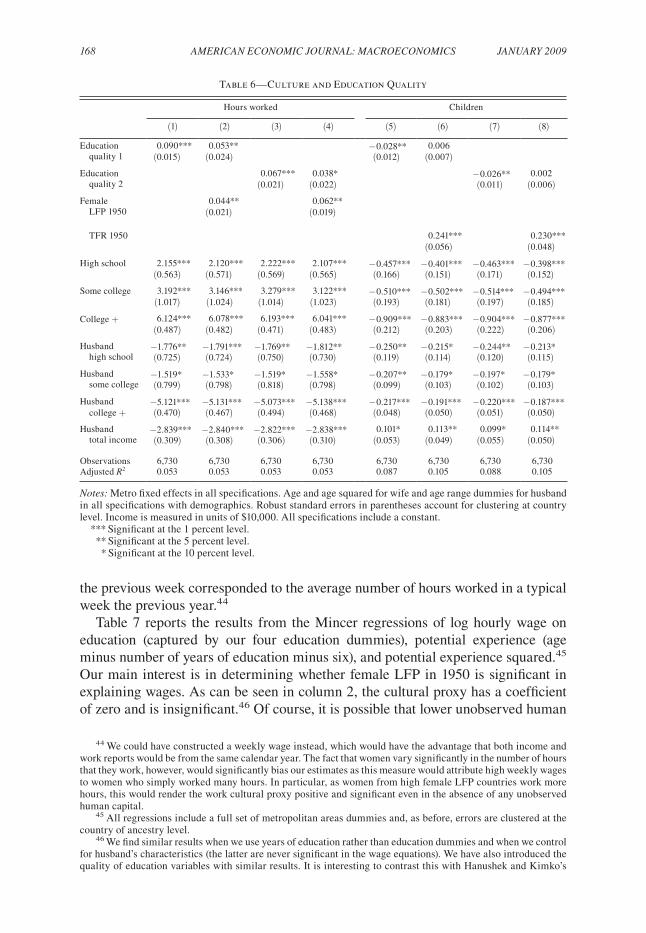
Table 6 reports the results of including education quality in our regressions. The significance of the education quality variable drops whenever the work cultural proxy is included in the specification and the latter remains positive and significant. A similar pattern can be noted for fertility, with education quality never significant once TFR 1950 is included.43

From the above, we can conclude that differences in education quality (whether in the form of unobserved human capital from parents or in the quality of the human capital in ethnic networks) are also not responsible for our results.

D. Wages

In this section, we take a more direct approach to unobserved human capital by examining women’s wages. If unobserved human capital is responsible for our results, it should be reflected as well in wages. In particular, if the cultural proxy were correlated with systematic differences in human capital by country of ancestry it should help explain variation in women’s wages. We show that this is not the case. We consider this a strong result in establishing that unobserved human capital is not responsible for our results.

We start by examining those women who work and declare positive earnings in order to run a standard Mincer regression. We would have liked to use the log of hourly wages as our dependent variable. This is not possible since income and hours worked correspond to different time periods. Census respondents report total pretax wage and salary income—that is, money received as an employee—for the previ-ous calendar year along with the weeks worked, but the hours reported are from the week preceding the interview. To deal with this problem, we construct a measure of hourly wages by dividing labor income by weeks worked multiplied by hours worked. This would coincide with the hourly wage if the number of hours worked

42 Hanushek and Kimko provide direct measures of quality for some 30 plus countries and then estimate a production function which they use to construct quality measures for another 40 or so countries for which test scores are not available. Our measures of quality do not distinguish between the two sets of countries. Note that individuals with ancestry from either Cuba and Lebanon are dropped from all regressions in this section as qual-ity measures were not available for them.

43 We also included education quality along with our measures of 1940 ethnic human capital. They were insig-nificant whereas the magnitude and significance of the cultural proxies were unaffected.


the previous week corresponded to the average number of hours worked in a typical week the previous year.44

Table 7 reports the results from the Mincer regressions of log hourly wage on education (captured by our four education dummies), potential experience (age minus number of years of education minus six), and potential experience squared.45 Our main interest is in determining whether female LFP in 1950 is significant in explaining wages. As can be seen in column 2, the cultural proxy has a coefficient of zero and is insignificant.46 Of course, it is possible that lower unobserved human

44 We could have constructed a weekly wage instead, which would have the advantage that both income and work reports would be from the same calendar year. The fact that women vary significantly in the number of hours that they work, however, would significantly bias our estimates as this measure would attribute high weekly wages to women who simply worked many hours. In particular, as women from high female LFP countries work more hours, this would render the work cultural proxy positive and significant even in the absence of any unobserved human capital.

45 All regressions include a full set of metropolitan areas dummies and, as before, errors are clustered at the country of ancestry level.

46 We find similar results when we use years of education rather than education dummies and when we control for husband’s characteristics (the latter are never significant in the wage equations). We have also introduced the quality of education variables with similar results. It is interesting to contrast this with Hanushek and Kimko’s

Table 6—Culture and Education Quality


(1) (2) (3) (4) (5) (6) (7) (8)

Education 0.090*** 0.053** −0.028** 0.006 quality 1 (0.015) (0.024) (0.012) (0.007)

Education 0.067*** 0.038* −0.026** 0.002 quality 2 (0.021) (0.022) (0.011) (0.006)

Female 0.044** 0.062** LFP 1950 (0.021) (0.019)

TFR 1950 0.241*** 0.230***(0.056) (0.048)

High school 2.155*** 2.120*** 2.222*** 2.107*** −0.457*** −0.401*** −0.463*** −0.398***(0.563) (0.571) (0.569) (0.565) (0.166) (0.151) (0.171) (0.152)

Some college 3.192*** 3.146*** 3.279*** 3.122*** −0.510*** −0.502*** −0.514*** −0.494***(1.017) (1.024) (1.014) (1.023) (0.193) (0.181) (0.197) (0.185)

College + 6.124*** 6.078*** 6.193*** 6.041*** −0.909*** −0.883*** −0.904*** −0.877***(0.487) (0.482) (0.471) (0.483) (0.212) (0.203) (0.222) (0.206)

Husband −1.776** −1.791*** −1.769** −1.812** −0.250** −0.215* −0.244** −0.213* high school (0.725) (0.724) (0.750) (0.730) (0.119) (0.114) (0.120) (0.115)

Husband −1.519* −1.533* −1.519* −1.558* −0.207** −0.179* −0.197* −0.179* some college (0.799) (0.798) (0.818) (0.798) (0.099) (0.103) (0.102) (0.103)

Husband −5.121*** −5.131*** −5.073*** −5.138*** −0.217*** −0.191*** −0.220*** −0.187*** college + (0.470) (0.467) (0.494) (0.468) (0.048) (0.050) (0.051) (0.050)

Husband −2.839*** −2.840*** −2.822*** −2.838*** 0.101* 0.113** 0.099* 0.114** total income (0.309) (0.308) (0.306) (0.310) (0.053) (0.049) (0.055) (0.050)

Observations 6,730 6,730 6,730 6,730 6,730 6,730 6,730 6,730Adjusted r2 0.053 0.053 0.053 0.053 0.087 0.105 0.088 0.105

Notes: Metro fixed effects in all specifications. Age and age squared for wife and age range dummies for husband in all specifications with demographics. Robust standard errors in parentheses account for clustering at country level. Income is measured in units of $10,000. All specifications include a constant. *** Significant at the 1 percent level. ** Significant at the 5 percent level. * Significant at the 10 percent level.


capital (and hence lower market wages) helps explain why some women are not participating in the labor market. The last two columns of Table 7 report the results obtained when wages are estimated with a Heckman selection model in which the husband’s characteristics are used to control for selection into employment.47 We find results very similar to those obtained for the restricted sample; the cultural vari-able is not significant in explaining hourly wages.48

V. Her or His Culture?

A married woman’s work and fertility outcomes are likely to be influenced not only by the factors that we have already explored—her age and education, her beliefs and preferences as embodied in the cultural proxies, and her husband’s characteris-tics—but also by the beliefs and preferences, (i.e., by the culture of her husband). In

findings. Although they find a significant positive effect of education quality in Mincer wage regressions for immigrants, these variables are no longer significant for the subsample of immigrants who obtained their school-ing in the United States. Our sample of women, of course, is more similar to this subsample as our women were born (and presumably educated) in the United States.

47 We find similar results when we use a dummy variable for whether a woman has a child under five years old in the selection equation.

48 We also imputed wages to nonworking women following Blau and Kahn (2005). We ran our baseline labor supply regressions and found that our cultural proxy remained significant.

Table 7—Culture and Wages

Log hourly wage

OLS Heckman

(1) (2) (3) (4)

Female LFP 1950 0.002 0.002

(0.002) (0.002)

High school 0.074*** 0.067** 0.081*** 0.073***(0.027) (0.025) (0.027) (0.025)

Some college 0.301*** 0.291*** 0.309*** 0.298***(0.050) (0.048) (0.049) (0.046)

College + 0.681*** 0.666*** 0.698*** 0.681***(0.061) (0.057) (0.063) (0.058)

Experience −0.017 −0.020 −0.013 −0.016(0.024) (0.024) (0.027) (0.026)

Experience squared 0.000 0.000 0.000 0.000(0.001) (0.001) (0.001) (0.001)

Observations 1,977 1,977 6,528 6,528Adjusted r2 0.103 0.103 Censored observations 4,551 4,551Log pseudo-likelihood −5,678 −5,675λ (= σρ) 0.056 0.053

Notes: Metro fixed effects in all specifications. Robust standard errors in parentheses account for clustering at country level. Income in units of $10,000. The selection equation also includes age and education dummies for husband and husband’s total income. *** Significant at the 1 percent level. ** Significant at the 5 percent level. * Significant at the 10 percent level.


this section, we wish to explore whether the husband’s cultural beliefs as to the role of women and family size affect his wife’s work and fertility outcomes. Of course, a woman’s culture, and that of her husband’s, are unlikely to be random. A woman who would like to work or would prefer a larger family is presumably more likely to marry a man who would be in agreement with these choices. Nonetheless, it is of interest to ask whether it is her culture or her husband’s culture or both that matter for these outcomes.49

To study the impact of the wife’s and husband’s cultures on a woman’s work and fertility outcomes, we include cultural proxies for both spouses, in each case assigned by the respective father’s country of birth. Note that many women will be married to men whose fathers were born in the United States. To these men, there-fore, we must associate US female LFP and TFR in 1950. In order to not have an asymmetric sample in which the US variables appear only when associated with a woman’s husband, we expand our sample to include women whose fathers were born in the United States but whose fathers-in-law are foreign-born. To do this, we follow the same procedure we described earlier. We drop those women whose father-in-law is from a European centrally planned economy or from a country for which we have fewer than 15 observations. Our final sample consists of 12,060 married women and 26 countries (including the United States).50 In this sample, 32.6 percent of women are married to men whose father was born in the United States (and thus these wom-en’s fathers were born elsewhere); 47.6 percent of the women have fathers born in the United States (and hence they are married to men with foreign-born fathers). The remaining 19.7 percent of women and their husbands both have fathers born outside the United States. Only 13.7 percent of the couples in our sample share the same cul-ture (i.e., have fathers born in the same country), though this is due to the fact that we have omitted those women with fathers and fathers-in-law born in the United States. If we were to restrict our attention to couples in which neither spouse has a father born in the United States, then 69.4 percent of these share the same culture.

To study the effect of the two spouses’ cultures, we distinguish between couples who share identical cultures (i.e., their fathers were born in the same country) from those with different cultures. We create two dummy variables: Same (for same cul-ture) and Not Same (for different cultures) and interact these with the cultural prox-ies. It should be noted that the number of observations for same culture is relatively small (1,653). The results of our regression analysis are reported for the full specifi-cation in Table 8.

The first column in Table 8 reports the results for hours worked using only the wife’s cultural proxy for work. As before, it is positive and statistically significant (for Not Same). The next column uses only the husband’s cultural proxy, which is also posi-tive and statistically significant. The third column uses both proxies. Interestingly, the coefficient on the husband’s cultural proxy is larger and more significant than that of his wife’s (which is significant at the 10 percent level). Furthermore, in this

49 Once one leaves the unitary household model, there is no reason to believe that husbands and wives neces-sarily share the same preferences over outcomes (see, e.g., Shelly Lundberg and Pollak 1996).

50 Another way of thinking about our sample selection is from the universe of married women born in the United States and between the ages of 30–40, we have eliminated those women who have both a US born father and a US born father-in-law.


last specification, the coefficient on the cultural proxy when the culture of the two spouses is the same is significant and larger than either of the two different cultures coefficients.

Columns 4 and 5 repeat the same specifications for fertility. The cultural proxy is positive and significant when it is the wife’s, the husband’s, and when both are simultaneously included. When the wife and husband share the same culture, the cultural proxy is also positive and significant, this time in all three specifications. The coefficients for each spouse separately are basically equal, as are the coeffi-cients for each spouse when they are entered jointly in the final specification. In this last specification, the sum of the coefficients on the wife’s and the husband’s cultural

Table 8—His or Her Culture?

Dependent variable is hours worked Dependent variable is children

(1) (2) (3) (4) (5) (6)

Same × female 0.027 0.035 0.070** LFP 1950 (0.026) (0.030) (0.034)

Not same × wife’s 0.058*** 0.044* female LFP 1950 (0.015) (0.023)

Not same × husband’s 0.067*** 0.058*** female LFP 1950 (0.020) (0.016)

Same × TFR 1950 0.216*** 0.214*** 0.312***(0.039) (0.044) (0.029)

Not same × wife’s 0.179*** 0.157*** TFR 1950 (0.036) (0.024)

Not same × husband’s 0.180*** 0.162*** TFR 1950 (0.042) (0.038)

High school 2.348*** 2.343*** 2.280*** −0.461*** −0.457*** −0.424***(0.304) (0.408) (0.365) (0.097) (0.100) (0.076)

Some college 3.542*** 3.552*** 3.463*** −0.500*** −0.491*** −0.466***(0.476) (0.509) (0.520) (0.099) (0.116) (0.092)

College + 6.344*** 6.320*** 6.230*** −0.949*** −0.939*** −0.911***(0.245) (0.493) (0.579) (0.124) (0.101) (0.097)

Husband −1.472*** −1.496*** −1.534*** −0.179*** −0.177** −0.155*** high school (0.421) (0.348) (0.365) (0.057) (0.074) (0.059)

Husband −1.523*** −1.587*** −1.612*** −0.173*** −0.167* −0.153** some college (0.427) (0.318) (0.505) (0.051) (0.086) (0.066)

Husband −4.541*** −4.574*** −4.611*** −0.166*** −0.178** −0.154** college + (0.434) (0.597) (0.474) (0.032) (0.088) (0.067)

Husband −3.161*** −3.188*** −3.192*** 0.134*** 0.140*** 0.141*** total income (0.206) (0.211) (0.233) (0.024) (0.038) (0.027)

Observations 12,060 12,060 12,060 12,060 12,060 12,060Adjusted r2 0.056 0.056 0.056 0.09 0.092 0.099

Notes: Metro fixed effects in all specifications. Age and age squared for wife and age range dummies for husband in all specifications with demographics. Robust standard errors in parentheses account for clustering at coun-try of own father × country of husband’s father level. Income is measured in units of $10,000. All specifications include a constant. *** Significant at the 1 percent level. ** Significant at the 5 percent level. * Significant at the 10 percent level.


proxies is essentially the same as the coefficient on cultural proxy when the spouses share the same culture.

We have also experimented with restricting our sample to the subset of women who have neither a US father nor a US father-in-law.51 The results are similar to the ones above except that for the work regressions the cultural proxy, when the couple shares the same culture, is now much larger, positive, and significant for all three specifications.

VI. Cultural Transmission

In this section, we bring additional evidence to bear on the hypothesis that culture is responsible for our results by investigating the role of neighborhood composition in cultural transmission. An individual’s neighborhood may play an important role in transmitting and preserving a set of beliefs or preferences, independently of the human capital embodied in an individual’s ethnic network. A neighborhood that has a relatively high proportion of individuals from the same ancestry may help preserve that country’s culture by punishing behavior that is different from the norm (by, for example, ostracizing the deviant individual). It may also keep the culture of the country of ancestry alive by providing role models and diffusing specific beliefs about how individuals, and in particular women, should act. In this section, we explore the role of neighborhoods in cultural transmission and preservation by investigating how the propensity of an ethnic group to cluster in the same neighbor-hood affects the impact of culture. The hypothesis is that the greater the proportion of an ethnic group in a neighborhood, the larger the effect of the cultural proxies on individual behavior. Note that this is a different type of “ethnic externality” from those explored by Borjas. Here, it is not the education of the ethnic group that is an input into the production of an individual’s human capital, but rather the greater presence of this group in a community that facilitates the transmission and preserva-tion of a particular set of beliefs, either through role models or through rewards and punishments.

To explore the role of ethnic density, we turn to data provided in Borjas (1995). Borjas calculates the extent of residential segregation for both first- and second-gen-eration Americans by estimating the proportion of the respondent’s neighborhood that is of the same ethnicity and then averaging this number across respondents.52 We use Borjas’ estimates of residential segregation for second-generation Americans to attach an average ethnic density to each country of ancestry.53 These numbers are reported by country of ancestry in Table 1.

As can be seen in Table 1, on average, second-generation Americans typically live in neighborhoods where the density of their own ethnic group is 4.3 percent with a standard deviation of 4.5 percent (i.e., the average second-generation American

51 There are 2,381 such observations.52 See Borjas (1995, table 2).53 Borjas does not include Spain, so individuals from this country of ancestry are excluded in the analysis

that follows. He also has separate entries for England, Wales, and Scotland, which we aggregate to one United Kingdom value by weighing each separate density figure by the proportion of UK observations in our sample that come from each of these three countries.


resides in a neighborhood in which 4.3 percent of the community is from the same ethnic group). Mexicans, Italians, and Japanese live in ethnically dense neigh-borhoods (respectively, 18.1, 12.1, and 12.6 percent), whereas Turks, French, and Lebanese live in neighborhoods with low ethnic density (0.3, 0.3, and 0.4 percent, respectively). Note that the ethnic density number depends on the extent to which members of an ethnic group cluster into the same neighborhoods and on how large that ethnic group is in the population (since if the ethnic group is not large, then even if they tended to cluster, this could show up as a low density number). In Table 1, the rank correlation of the number of observations by country of ancestry and ethnic density is 0.5, showing that both elements probably play a role. In any case, from the perspective of cultural transmission, it may not matter which variable is the source of ethnic density.

In order to explore the effect of ethnic density, we include density, the cultural proxy, and density interacted with the culture proxy in our regression analysis both separately and jointly. Columns 1–3 and 4–5 of Table 9 report the effects for hours worked and fertility, respectively. Across all specifications, density is significant only if the culture proxy variable is also included. Note that the interaction of culture and density is positive and significant. Moreover, the full marginal effects of female LFP 1950 and TFR 1950 remain positive and significant, whereas the full marginal effect of density is insignificantly different from zero when evaluated at the mean. A one standard deviation increase in female LFP 1950 is associated with a 0.76 increase in hours worked (evaluated at the mean of density). A one standard deviation increase in TFR 1950 is associated with a 0.19 increase in the number of children.

From the above, we conclude that the degree to which ethnic groups cluster in the same neighborhoods appears to be an important mechanism in maintaining culture.The greater the average density of an ethnic group, the greater the impact of culture on a woman’s work and fertility outcomes.54 Whether this is due to role models and enhanced transmission (voluntary or involuntary) of a particular set of preferences or beliefs or due to the greater capacity for reward and punishment of a larger social group is an interesting question which should be investigated in future work.

VII. Conclusion

This paper argues that culture matters to important economic outcomes, namely, female work and fertility. We show that female LFP and TFR in 1950 by coun-try of ancestry, our cultural proxies, are economically and statistically significant in explaining how much women work and how many children they have. We also examine the most likely suspects that could be responsible for our results. In par-ticular, we have shown that neither unobserved human capital nor network quality is likely to be a driving force. On the other hand, we find that the average propensity of an ethnic group to cluster in the same neighborhood magnifies the impact of the cul-tural proxies on work and fertility, which is consistent with the theory that cultural transmission occurs through the family and neighborhood.

54 Whether this has positive or negative welfare effects depends on one’s view about the validity of the under-lying beliefs.


There are, of course, other possible interpretations of the empirical evidence we provided. For example, if household skills are transmitted primarily from mothers to daughters and if these are higher for mothers who do not work, then the traditional comparative advantage argument may help explain why the daughters of women from low female LFP countries tend to work less. This alternative hypothesis, how-ever, would not explain why the impact of the cultural proxy is stronger the greater the propensity of the ethnic group to cluster into neighborhoods.

Another hypothesis is that there are varying degrees of discrimination in the US labor market that (negatively) correlate with female LFP in the country of ancestry. We do not think that such a correlation is very plausible for two reasons. First, we do not see this pattern for men by country of ancestry (see Fernández and Fogli 2005). This implies that if discrimination (in hiring) is responsible for the observed pattern of results, it would have to be faced only by the women and not by the men

Table 9—Culture and Ethnic Density


(1) (2) (3) (4) (5) (6)

Density −0.047 0.021 −0.124** 0.023 0.001 −0.056***(0.036) (0.036) (0.055) (0.022) (0.013) (0.014)

Density × female 0.008*** 0.016*** LFP 1950 (0.003) (0.004)

Female 0.079*** 0.033 LFP 1950 (0.025) (0.026)

TFR 1950 0.217*** 0.035(0.056) (0.072)

High school 2.274*** 2.174*** 2.058*** −0.474*** −0.395*** −0.356**(0.561) (0.564) (0.565) (0.164) (0.145) (0.141)

Some college 3.414*** 3.291*** 3.192*** −0.524*** −0.480*** −0.447***(1.001) (1.019) (1.036) (0.181) (0.171) (0.171)

College + 6.213*** 6.072*** 5.946*** −0.928*** −0.862*** −0.820***(0.543) (0.508) (0.494) (0.208) (0.196) (0.193)

Husband −1.704** −1.763** −1.836** −0.275** −0.220* −0.201* high school (0.751) (0.742) (0.729) (0.121) (0.113) (0.112)

Husband −1.368* −1.401* −1.461* −0.225** −0.187* −0.172* some college (0.822) (0.825) (0.814) (0.093) (0.101) (0.100)

Husband −5.012*** −5.057*** −5.114*** −0.261*** −0.213*** −0.203*** college + (0.473) (0.460) (0.461) (0.045) (0.045) (0.045)

Husband −2.859*** −2.860*** −2.876*** 0.106** 0.120** 0.125*** total income (0.309) (0.308) (0.305) (0.049) (0.047) (0.046)

Observations 6,709 6,709 6,709 6,709 6,709 6,709Adjusted r2 0.052 0.053 0.053 0.082 0.104 0.111

Notes: Metro fixed effects in all specifications. Age and age squared for wife and age range dummies for husband in all specifications with demographics. Robust standard errors in parentheses account for clustering at country level. Income is measured in units of $10,000. All specifications include a constant. *** Significant at the 1 percent level. ** Significant at the 5 percent level. * Significant at the 10 percent level.


from these countries, which seems rather implausible Second, when we differentiate between the effects of the wife’s and husband’s cultures on the work behavior of the wife, the husband’s culture is more significant and has a greater impact (see Section V). Thus, it is unlikely that employers are discriminating on the basis of a woman’s ethnic characteristics as, in that case, the husband’s characteristics should not be particularly relevant.55

We think that our estimates of the quantitative impact of culture are likely to underestimate its true importance. Indeed, we find it telling that despite the fact that we study the work and fertility behavior of second-generation immigrants to the United States (who are likely never to have set foot in their father’s country of ancestry), and despite the fact that we control for most of the indirect effects of cul-ture, we find the direct effect of our cultural proxies to be quantitatively significant. We think, therefore, that culture plays an important role in explaining the large variation across time and countries in women’s work and fertility. Moreover, there is no reason to believe that culture’s impact is restricted to the variables we studied. Culture is also likely to play a role in explaining cross-country variation in other key individual economic outcomes such as entrepreneurial activity, creativity, and physi-cal and human capital accumulation. Culture, therefore, is too important an area for economists to ignore.

55 Note, furthermore, that our sample is overwhelmingly European so it is doubtful that discrimination is occurring on the basis of skin color, for example.

Appendix

Table A1—Individual Summary Statistics

Census GSS

Variable MeanStandard deviation Minimum Maximum Mean

Standard deviation Minimum Maximum

Hours worked 10.19 16.31 0 66Weeks worked 15.21 20.91 0 51Full time 0.31 0.46 0 1Children 3.07 1.82 0 12 2.51 1.57 0 8Age 35.69 3.16 30 40 38.20 6.49 29 50High school 0.53 0.50 0 1 0.49 0.50 0 1Some college 0.11 0.31 0 1 0.16 0.37 0 1College + 0.08 0.28 0 1 0.18 0.39 0 1Husband high school 0.35 0.48 0 1 0.34 0.47 0 1Husband some college 0.13 0.33 0 1 0.21 0.41 0 1Husband college + 0.20 0.40 0 1 0.24 0.43 0 1Husband age 39.00 6.00 14 100 40.17 8.84 19 99Husband total income 1.13 0.68 −0.99 5 3.41 2.67 −0.73 16.26

Notes: Census: there are 6,774 married couples in our sample. Data are from 1 percent 1970 Form 2 Metro Sample of the US Census. The sample includes married women 30–40 year old not living in farms or group quarters and not working in agricul-tural occupations, whose fathers were born in one of the 25 countries in our sample. Income is measured in units of $10,000. GSS: There are 456 married couples in our sample. Data are from the GSS for years 1977, 1978, 1980, and 1982. The sample includes married women 29–50 years old, born in the United States whose ancestors came from one of the nine countries in our sample. Income is measured in units of $10,000.


REFERENCES

Algan, Yann, and Pierre Cahuc. 2005. “The Roots of Low European Employment: Family Culture?” In NBEr international Seminar on Macroeconomics 2005, ed. Jeffrey Frankel and Christopher Pissarides, 65–109. Cambridge, MA: MIT Press, (2007).

Algan, Yann, and Pierre Cahuc. 2006. “Civic Attitudes and the Design of Labor Market Institutions (IZA): Which Countries can Implement the Danish Flexicurity Model?” Institute for the Study of Labor Working Paper 1928.

Antecol, Heather. 2000. “An Examination of Cross-Country Differences in the Gender Gap in Labor Force Participation Rates.” Labour Economics, 7(4): 409–26.

Barro, Robert J., and Rachel McCleary. 2003. “Religion and Economic Growth.” American Socio-logical review, 68(5): 760–81.

Blau, Francine D. 1992. “The Fertility of Immigrant Women: Evidence from High- Fertility Source Countries.” In immigration and the Workforce: Economic Consequences for the United States and Source Areas, ed. George J. Borjas and Richard B. Freeman, 93–134. Chicago: University of Chicago Press.

Blau, Francine D., and Lawrence M. Kahn. 2005. “Changes in the Labor Supply Behavior of Married Women: 1980-2000.” National Bureau of Economic Research Working Paper 11230.

Blau, Francine D., and Lawrence M. Kahn. 2007. “Gender and Assimilation among Mexican Ameri-cans.” In Mexican immigration to the United States. National Bureau of Economic research Con-ference report, ed. George J. Borjas, 57–106. Chicago, IL: University of Chicago Press.

Borjas, George J. 1992. “Ethnic Capital and Intergenerational Mobility.” Quarterly Journal of Eco-nomics, 107(1): 123–150.

Borjas, George J. 1995. “Ethnicity, Neighborhoods, and Human-Capital Externalities.” American Economic review, 85(3): 365–90.

Borjas, George J. 2007. “Introduction.” In Mexican immigration to the United States. National Bureau of Economic research Conference report, ed. George J. Borjas, 1–12. Chicago: Univer-sity of Chicago Press.

Botticini, Maristella, and Zvi Eckstein. 2005. “Jewish Occupational Selection: Education, Restric-tions, or Minorities?” Journal of Economic History, 65(4): 922–48.

Carroll, Christopher D., Byung-Kun Rhee, and Changyong Rhee. 1994. “Are There Cultural Effects on Saving? Some Cross-Sectional Evidence.” Quarterly Journal of Economics, 109(3): 685–99.

Davis, James A., Tom W. Smith, and Peter V. Marsden. 1999. general Social Surveys, 1972-1998: Cumulative Codebook, Chicago: NORC.

Fernández, Raquel. 2008. “Culture and Economics.” In New Palgrave dictionary of Economics. 2nd edition, ed. Steven N. Durlauf and Lawrence E. Blume. New York, NY: Palrave and Macmillian.

Fernández, Raquel, Alessandra Fogli, and Claudia Olivetti. 2004. “Mothers and Sons: Preference For-mation and Female Labor Force Dynamics.” Quarterly Journal of Economics, 119(4): 1249–99.

Fernández, Raquel, Nezih Guner, and John Knowles. 2005. “Love and Money: A Theoretical and Empirical Analysis of Household Sorting and Inequality.” Quarterly Journal of Economics, 120(1): 273–344.

Fortin, Nicole M. 2005. “Gender Role Attitudes and the Labour-Market Outcomes of Women across OECD Countries.” oxford review of Economic Policy, 21(3): 416–38.

Giuliano, Paola. 2007. “Living Arrangements in Western Europe: Does Cultural Origin Matter?” Journal of the European Economic Association, 5(5): 927–52.

Gjerde, Jon, and Anne McCants. 1995. “Fertility, Marriage and Culture: Demographic Processes Among Norwegian Immigrants to the Rural Middle West.” Journal of Economic History, 55(4): 860–88.

Greif, Avner. 1994. “Cultural Beliefs, and the Organization of Society: a Historical and Theoreti-cal Reflection on Collectivist and Individualist Societies.” Journal of Political Economy, 102(5): 912–50.

Guinnane, Timothy W., Carolyn M. Moehling, and Cormac Ó Grada. 2006. “The Fertility of the Irish in America in 1910.” Explorations in Economic History, 43(3): 465–85.

Guiso, Luigi, Paola Sapienza, and Luigi Zingales. 2004. “Cultural Biases in Economic Exchange.” National Bureau of Economic Research Working Paper 11005.

Hanushek, Eric A., and Dennis D. Kimko. 2000. “Schooling, Labor-Force Quality, and the Growth of Nations.” American Economic review, 90(5): 1184–1208.

International Labour Office. 1988. Current International Recommendations on Labour Statistics. Geneva: International Labour Organization.


Kroeber, A. L., and Clyde Kluckhohn. 1952. Culture: A Critical review of Concepts and definitions. Cambridge, MA: Peabody Museum.

Landes, David S. 1998. The Wealth and Poverty of Nations: Why Some are so rich and Some so Poor. New York: W. W. Norton.

Levine, David I. 1993. “The Effect of Non-Traditional Attitudes on Married Women’s Labor Supply.” Journal of Economic Psychology, 14(4): 665–79.

Lundberg, Shelly, and Robert A. Pollak. 1996. “Bargaining and Distribution in Marriage.” Journal of Economic Perspectives, 10(4): 139–58.

Pencavel, John. 1998. “The Market Work Behavior and Wages of Women: 1975-94.” Journal of Human resources, 38(4): 771–804.

Pollak, Robert A., and Susan Cotts Watkins. 1993. “Cultural and Economic Approaches to Fertility:Proper Marriage or Mesalliance?” Population and development review, 19(3): 467–96.

Putnam, Robert D. 2000. Bowling Alone: The Collapse and revival of American Community. New York: Simon and Schuster.

Reimers, Cordelia W. 1985. “Cultural Differences in Labor Force Participation among Married Women.” American Economic review, 75(2): 251–55.

Stigler, George J., and Gary S. Becker. 1977. “De Gustibus Non Est Disputandum.” American Eco-nomic review, 67(2): 76–90.

Tabellini, Guido. 2005. “Culture and Institutions: Economic Development in the Regions of Europe.” CESifo Working Paper 1492.

Vella, Francis. 1994, “Gender Roles and Human Capital Investment: The Relationship between Tradi-tional Attitudes and Female Labour Market Performance.” Economica, 61(242): 191–211.

Weil, David N. 2004. Economic growth, Boston: Addison-Wesley.

Documents

Culture: An Empirical Investigation of Beliefs, Work, and ... · 3 In their famous 1952 book, anthropologists A. L. Kroeber and Clyde Kluckhohn cited 164 definitions of culture. Without