Embed Size (px)
Citation preview
DG-05603-001_v4.0 | May 2011
Design Guide
CUDA C BEST PRACTICES GUIDE
www.nvidia.com
CUDA C Best Practices Guide DG-05603-001_v4.0 | ii
DOCUMENT CHANGE HISTORY
DG-05603-001_v4.0
Version Date Authors Description of Change
3.0 February 4, 2010 CW See Section C.1
3.1 May 19, 2010 CW See Section C.2
3.2 August 20, 2010 CW See Section C.3
4.0 May 9, 2011 CW,NJ,VS See Section C.4
www.nvidia.com
CUDA C Best Practices Guide DG-05603-001_v4.0 | iii
TABLE OF CONTENTS
Preface ........................................................................................................... 1
What is This Document? ..................................................................................... 1
Who Should Read This Guide? .............................................................................. 1
Recommendations and Best Practices ..................................................................... 2
Contents ........................................................................................................ 2
Chapter 1. Parallel Computing with CUDA ......................................................... 4
1.1 Heterogeneous Computing with CUDA ............................................................. 4
1.1.1 Differences Between Host and Device ..................................................... 4
1.1.2 What Runs on a CUDA-Enabled Device? ................................................... 5
1.1.3 Maximum Performance Benefit .............................................................. 7
1.2 Understanding the Programming Environment ................................................... 7
1.2.1 CUDA Compute Capability .................................................................... 8
1.2.2 Additional Hardware Data .................................................................... 8
1.2.3 CUDA Runtime and CUDA Driver API Version............................................. 9
1.2.4 Which Version to Target ...................................................................... 9
1.3 CUDA APIs ............................................................................................. 10
1.3.1 CUDA Runtime API ........................................................................... 11
1.3.2 CUDA Driver API .............................................................................. 11
1.3.3 When to Use Which API ..................................................................... 11
1.3.4 Comparing Code for Different APIs ........................................................ 12
Chapter 2. Performance Metrics .................................................................... 15
2.1 Timing .................................................................................................. 15
2.1.1 Using CPU Timers ............................................................................ 15
2.1.2 Using CUDA GPU Timers .................................................................... 16
2.2 Bandwidth .............................................................................................. 17
2.2.1 Theoretical Bandwidth Calculation ......................................................... 17
2.2.2 Effective Bandwidth Calculation ............................................................ 18
2.2.3 Throughput Reported by cudaprof ........................................................ 18
Chapter 3. Memory Optimizations .................................................................. 19
3.1 Data Transfer Between Host and Device ......................................................... 19
3.1.1 Pinned Memory ............................................................................... 20
3.1.2 Asynchronous Transfers and Overlapping Transfers with Computation ............. 20
3.1.3 Zero Copy ...................................................................................... 23
3.2 Device Memory Spaces .............................................................................. 24
3.2.1 Coalesced Access to Global Memory ...................................................... 25
3.2.2 Shared Memory ............................................................................... 31
3.2.3 Local Memory ................................................................................. 38
3.2.4 Texture Memory .............................................................................. 39
3.2.5 Constant Memory ............................................................................. 42
3.2.6 Registers ....................................................................................... 42
3.3 Allocation ............................................................................................... 43
www.nvidia.com
CUDA C Best Practices Guide DG-05603-001_v4.0 | iv
Chapter 4. Execution Configuration Optimizations ........................................... 44
4.1 Occupancy ............................................................................................. 44
4.2 Calculating Occupancy ............................................................................... 45
4.3 Hiding Register Dependencies ...................................................................... 46
4.4 Thread and Block Heuristics ........................................................................ 47
4.5 Effects of Shared Memory ........................................................................... 48
Chapter 5. Instruction Optimizations ............................................................. 50
5.1 Arithmetic Instructions ............................................................................... 50
5.1.1 Division and Modulo Operations ........................................................... 50
5.1.2 Reciprocal Square Root ...................................................................... 51
5.1.3 Other Arithmetic Instructions ............................................................... 51
5.1.4 Math Libraries ................................................................................. 51
5.2 Memory Instructions ................................................................................. 54
Chapter 6. Control Flow ............................................................................... 55
6.1 Branching and Divergence .......................................................................... 55
6.2 Branch Predication .................................................................................... 56
6.3 Loop counters signed vs. unsigned ................................................................ 56
Chapter 7. Getting the Right Answer .............................................................. 58
7.1 Debugging ............................................................................................. 58
7.2 Numerical Accuracy and Precision ................................................................. 58
7.2.1 Single vs. Double Precision ................................................................. 59
7.2.2 Floating-Point Math Is Not Associative .................................................... 59
7.2.3 Promotions to Doubles and Truncations to Floats ...................................... 59
7.2.4 IEEE 754 Compliance ........................................................................ 60
7.2.5 x86 80-bit Computations .................................................................... 60
Chapter 8. Multi-GPU Programming ............................................................... 61
8.1 Introduction to Multi-GPU ........................................................................... 61
8.2 Multi-GPU Programming ............................................................................. 61
8.3 Selecting a GPU ....................................................................................... 62
8.4 Inter-GPU communication ........................................................................... 63
8.5 Compiling Multi-GPU Applications .................................................................. 63
8.6 Infiniband .............................................................................................. 64
Appendix A. Recommendations and Best Practices .......................................... 65
A.1 Overall Performance Optimization Strategies .................................................. 65
A.2 High-Priority Recommendations .................................................................. 66
A.3 Medium-Priority Recommendations .............................................................. 66
A.4 Low-Priority Recommendations .................................................................. 67
Appendix B. NVCC Compiler Switches ............................................................ 68
B.1 NVCC ................................................................................................. 68
Appendix C. Revision History ....................................................................... 69
C.1 Version 3.0........................................................................................... 69
C.2 Version 3.1........................................................................................... 70
C.3 Version 3.2........................................................................................... 70
C.4 Version 4.0........................................................................................... 70
www.nvidia.com
CUDA C Best Practices Guide DG-05603-001_v4.0 | v
LIST OF FIGURES
Figure 1.1. Sample CUDA Configuration Data Reported by deviceQuery .............................. 8
Figure 1.2. Compatibility of CUDA versions ................................................................. 9
Figure 3.1. Timeline Comparison for Sequential (top) and Concurrent (bottom) Copy and Kernel Execution ................................................................................. 22
Figure 3.2. Memory Spaces on a CUDA Device ........................................................... 24
Figure 3.3. Linear Memory Segments and Threads in a Half Warp .................................... 25
Figure 3.4. Coalesced Access–All Threads but One Access the Corresponding Word in a Segment ........................................................................................... 26
Figure 3.5. Unaligned Sequential Addresses that Fit within a Single 128-Byte Segment........... 27
Figure 3.6. Misaligned Sequential Addresses that Fall within Two 128-Byte Segments ............ 27
Figure 3.7. Performance of offsetCopy kernel ............................................................. 28
Figure 3.8. A half warp accessing memory with a stride of 2 .......................................... 30
Figure 3.9. Performance of strideCopy Kernel ............................................................ 30
Figure 3.10. Block-Column Matrix (A) Multiplied by Block-Row Matrix (B) with Resulting Product Matrix (C) ......................................................................................... 33
Figure 3.11. Computing a Row (Half Warp) of a Tile In C Using One Row of A and an Entire Tile of B ........................................................................................... 34
Figure 3.12. Results of Using Texture Memory to Avoid Uncoalesced Global Memory Access ...... 41
Figure 4.1. CUDA GPU Occupancy Calculator Usage to Project Occupancy .......................... 46
LIST OF TABLES
Table 3.1 Salient Features of Device Memory ........................................................... 24
Table 3.2 Performance Improvements Optimizing C = AB Matrix Multiply ......................... 36
Table 3.3 Performance Improvements Optimizing C = AAT Matrix Multiplication.................. 38
Table 3.4 Useful Features for tex1D(), tex2D(), and tex3D() Fetches .............................. 41
www.nvidia.com
CUDA C Best Practices Guide DG-05603-001_v4.0 | 1
PREFACE
WHAT IS THIS DOCUMENT?
This Best Practices Guide is a manual to help developers obtain the best performance
from the NVIDIA® CUDA™ architecture using version 4.0 of the CUDA Toolkit. It
presents established optimization techniques and explains coding metaphors and idioms
that can greatly simplify programming for the CUDA architecture.
While the contents can be used as a reference manual, you should be aware that some
topics are revisited in different contexts as various programming and configuration
topics are explored. As a result, it is recommended that first-time readers proceed
through the guide sequentially. This approach will greatly improve your understanding
of effective programming practices and enable you to better use the guide for reference
later.
WHO SHOULD READ THIS GUIDE?
This guide is intended for programmers who have a basic familiarity with the CUDA
programming environment. You have already downloaded and installed the CUDA
Toolkit and have written successful programs using it. The discussions in this guide all
use the C programming language, so you should be comfortable reading C.
This guide refers to and relies on several other documents that you should have at your
disposal for reference, all of which are available at no cost from the CUDA website
http:/www.nvidia.com/object/cuda_develop.html. The following documents are
especially important resources:
CUDA Quickstart Guide
CUDA C Programming Guide
Parallel Computing with CUDA
www.nvidia.com
CUDA C Best Practices Guide DG-05603-001_v4.0 | 2
CUDA Reference Manual
Be sure to download the correct manual for the CUDA Toolkit version and operating
system you are using.
RECOMMENDATIONS AND BEST PRACTICES
Throughout this guide, specific recommendations are made regarding the design and
implementation of CUDA C code. These recommendations are categorized by priority,
which is a blend of the effect of the recommendation and its scope. Actions that present
substantial improvements for most CUDA applications have the highest priority, while
small optimizations that affect only very specific situations are given a lower priority.
Before implementing lower priority recommendations, it is good practice to make sure
all higher priority recommendations that are relevant have already been applied. This
approach will tend to provide the best results for the time invested and will avoid the
trap of premature optimization.
The criteria of benefit and scope for establishing priority will vary depending on the
nature of the program. In this guide, they represent a typical case. Your code might
reflect different priority factors. Regardless of this possibility, it is good practice to verify
that no higher-priority recommendations have been overlooked before undertaking
lower-priority items.
Appendix A of this document lists all the recommendations and best practices, grouping
them by priority and adding some additional helpful observations.
Code samples throughout the guide omit error checking for conciseness. Production
code should, however, systematically check the error code returned by each API call and
check for failures in kernel launches (or groups of kernel launches in the case of
concurrent kernels) by calling cudaGetLastError().
CONTENTS
The remainder of this guide is divided into the following sections:
Parallel Computing with CUDA: Important aspects of the parallel programming
architecture.
Performance Metrics: How should performance be measured in CUDA applications
and what are the factors that most influence performance?
Memory Optimizations: Correct memory management is one of the most effective
means of improving performance. This chapter explores the different kinds of
memory available to CUDA applications.
Parallel Computing with CUDA
www.nvidia.com
CUDA C Best Practices Guide DG-05603-001_v4.0 | 3
Execution Configuration Optimizations: How to make sure your CUDA application is
exploiting all the available resources on the GPU.
Instruction Optimizations: Certain operations run faster than others. Using faster
operations and avoiding slower ones often confers remark¬able benefits.
Control Flow: Carelessly designed control flow can force parallel code into serial
execution; whereas thoughtfully designed control flow can help the hardware
perform the maximum amount of work per clock cycle.
Getting the Right Answer: How to debug code and how to handle differences in how
the CPU and GPU represent floating-point values.
www.nvidia.com
CUDA C Best Practices Guide DG-05603-001_v4.0 | 4
Chapter 1. PARALLEL COMPUTING WITH CUDA
This chapter reviews heterogeneous computing with CUDA, explains the limits of
performance improvement, and helps you choose the right version of CUDA and which
application programming interface (API) to use when programming.
1.1 HETEROGENEOUS COMPUTING WITH CUDA
CUDA C programming involves running code on two different platforms concurrently:
a host system with one or more CPUs and one or more devices (frequently graphics
adapter cards) with CUDA-enabled NVIDIA GPUs.
While NVIDIA devices are frequently associated with rendering graphics, they are also
powerful arithmetic engines capable of running thousands of lightweight threads in
parallel. This capability makes them well suited to computations that can leverage
parallel execution well.
However, the device is based on a distinctly different design from the host system, and
it’s important to understand those differences and how they determine the performance
of CUDA applications to use CUDA effectively.
1.1.1 Differences Between Host and Device
The primary differences occur in threading and memory access:
Threading resources. Execution pipelines on host systems can support a limited
number of concurrent threads. Servers that have four quad-core processors today can
run only 16 threads concurrently (32 if the CPUs support HyperThreading.) By
comparison, the smallest executable unit of parallelism on a CUDA device comprises
Parallel Computing with CUDA
www.nvidia.com
CUDA C Best Practices Guide DG-05603-001_v4.0 | 5
32 threads (a warp). All NVIDIA GPUs can support at least 768 concurrently active
threads per multiprocessor, and some GPUs support 1,024 or more active threads per
multiprocessor (see Section F.1 of the CUDA C Programming Guide). On devices that
have 30 multiprocessors (such as the NVIDIA® GeForce® GTX 280), this leads to more
than 30,000 active threads.
Threads. Threads on a CPU are generally heavyweight entities. The operating system
must swap threads on and off of CPU execution channels to provide multithreading
capability. Context switches (when two threads are swapped) are therefore slow and
expensive. By comparison, threads on GPUs are extremely lightweight. In a typical
system, thousands of threads are queued up for work (in warps of 32 threads each). If
the GPU must wait on one warp of threads, it simply begins executing work on
another. Because separate registers are allocated to all active threads, no swapping of
registers or state need occur between GPU threads. Resources stay allocated to each
thread until it completes its execution.
RAM. Both the host system and the device have RAM. On the host system, RAM is
generally equally accessible to all code (within the limitations enforced by the
operating system). On the device, RAM is divided virtually and physically into
different types, each of which has a special purpose and fulfills different needs. The
types of device RAM are explained in the CUDA C Programming Guide and in Chapter
3 of this document.
These are the primary hardware differences between CPU hosts and GPU devices with
respect to parallel programming. Other differences are discussed as they arise elsewhere
in this document.
1.1.2 What Runs on a CUDA-Enabled Device?
Because of the considerable differences between the host and the device, it’s important
to partition applications so that each hardware system is doing the work it does best.
The following issues should be considered when determining what parts of an
application to run on the device:
The device is ideally suited for computations that can be run on numerous data
elements simultaneously in parallel. This typically involves arithmetic on large data
sets (such as matrices) where the same operation can be performed across thousands,
if not millions, of elements at the same time. This is a requirement for good
performance on CUDA: the software must use a large number of threads. The
support for running numerous threads in parallel derives from the CUDA
architecture’s use of a lightweight threading model.
There should be some coherence in memory access by device code. Certain memory
access patterns enable the hardware to coalesce groups of reads or writes of multiple
data items into one operation. Data that cannot be laid out so as to enable coalescing,
or that doesn’t have enough locality to use textures or L1 efficiently, will not enjoy
much of a performance benefit when used in computations on CUDA.
Parallel Computing with CUDA
www.nvidia.com
CUDA C Best Practices Guide DG-05603-001_v4.0 | 6
To use CUDA, data values must be transferred from the host to the device along the
PCI Express (PCIe) bus. These transfers are costly in terms of performance and should
be minimized. (See Section 3.1.) This cost has several ramifications:
● The complexity of operations should justify the cost of moving data to and from
the device. Code that transfers data for brief use by a small number of threads will
see little or no performance benefit. The ideal scenario is one in which many
threads perform a substantial amount of work.
For example, transferring two matrices to the device to perform a matrix addition
and then transferring the results back to the host will not realize much
performance benefit. The issue here is the number of operations performed per
data element transferred. For the preceding procedure, assuming matrices of size
N×N, there are N2 operations (additions) and 3N2 elements transferred, so the ratio
of operations to elements transferred is 1:3 or O(1). Performance benefits can be
more readily achieved when this ratio is higher. For example, a matrix
multiplication of the same matrices requires N3 operations (multiply-add), so the
ratio of operations to elements transferred is O(N), in which case the larger the
matrix the greater the performance benefit. The types of operations are an
additional factor, as additions have different complexity profiles than, for example,
trigonometric functions. It is important to include the overhead of transferring
data to and from the device in determining whether operations should be
performed on the host or on the device.
● Data should be kept on the device as long as possible. Because transfers should be
minimized, programs that run multiple kernels on the same data should favor
leaving the data on the device between kernel calls, rather than transferring
intermediate results to the host and then sending them back to the device for
subsequent calculations. So, in the previous example, had the two matrices to be
added already been on the device as a result of some previous calculation, or if the
results of the addition would be used in some subsequent calculation, the matrix
addition should be performed locally on the device. This approach should be used
even if one of the steps in a sequence of calculations could be performed faster on
the host. Even a relatively slow kernel may be advantageous if it avoids one or
more PCIe transfers. Section 3.1 provides further details, including the
measurements of bandwidth between the host and the device versus within the
device proper.
Parallel Computing with CUDA
www.nvidia.com
CUDA C Best Practices Guide DG-05603-001_v4.0 | 7
1.1.3 Maximum Performance Benefit
High Priority: To get the maximum benefit from CUDA, focus first on finding ways to parallelize sequential code.
The amount of performance benefit an application will realize by running on CUDA
depends entirely on the extent to which it can be parallelized. As mentioned previously,
code that cannot be sufficiently parallelized should run on the host, unless doing so
would result in excessive transfers between the host and the device.
Amdahl’s law specifies the maximum speed-up that can be expected by parallelizing
portions of a serial program. Essentially, it states that the maximum speed-up (S) of a
program is :
where P is the fraction of the total serial execution time taken by the portion of code that
can be parallelized and N is the number of processors over which the parallel portion of
the code runs.
The larger N is (that is, the greater the number of processors), the smaller the P/N
fraction. It can be simpler to view N as a very large number, which essentially
transforms the equation into S = 1 / 1 P. Now, if ¾ of a program is parallelized, the
maximum speed-up over serial code is 1 / (1 – ¾) = 4.
For most purposes, the key point is that the greater P is, the greater the speed-up. An
additional caveat is implicit in this equation, which is that if P is a small number (so not
substantially parallel), increasing N does little to improve performance. To get the
largest lift, best practices suggest spending most effort on increasing P; that is, by
maximizing the amount of code that can be parallelized.
1.2 UNDERSTANDING THE PROGRAMMING ENVIRONMENT
With each generation of NVIDIA processors, new features are added to the GPU that
CUDA can leverage. Consequently, it’s important to understand the characteristics of
the architecture.
Programmers should be aware of two version numbers. The first is the compute
capability, and the second is the version number of the CUDA Runtime and CUDA
Driver APIs.
Parallel Computing with CUDA
www.nvidia.com
CUDA C Best Practices Guide DG-05603-001_v4.0 | 8
1.2.1 CUDA Compute Capability
The compute capability describes the features of the hardware and reflects the set of
instructions supported by the device as well as other specifications, such as the
maximum number of threads per block and the number of registers per multiprocessor.
Higher compute capability versions are supersets of lower (that is, earlier) versions, and
so they are backward compatible.
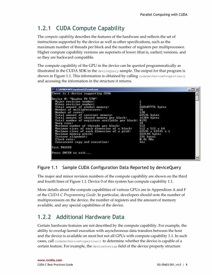
The compute capability of the GPU in the device can be queried programmatically as
illustrated in the CUDA SDK in the deviceQuery sample. The output for that program is
shown in Figure 1.1. This information is obtained by calling cudaGetDeviceProperties()
and accessing the information in the structure it returns.
Figure 1.1 Sample CUDA Configuration Data Reported by deviceQuery
The major and minor revision numbers of the compute capability are shown on the third
and fourth lines of Figure 1.1. Device 0 of this system has compute capability 1.1.
More details about the compute capabilities of various GPUs are in Appendices A and F
of the CUDA C Programming Guide. In particular, developers should note the number of
multiprocessors on the device, the number of registers and the amount of memory
available, and any special capabilities of the device.
1.2.2 Additional Hardware Data
Certain hardware features are not described by the compute capability. For example, the
ability to overlap kernel execution with asynchronous data transfers between the host
and the device is available on most but not all GPUs with compute capability 1.1. In such
cases, call cudaGetDeviceProperties() to determine whether the device is capable of a
certain feature. For example, the deviceOverlap field of the device property structure
Parallel Computing with CUDA
www.nvidia.com
CUDA C Best Practices Guide DG-05603-001_v4.0 | 9
indicates whether overlapping kernel execution and data transfers is possible (displayed
in the “Concurrent copy and execution” line of Figure 1.1); likewise, the
canMapHostMemory field indicates whether zero-copy data transfers can be performed.
1.2.3 CUDA Runtime and CUDA Driver API Version
The CUDA Driver API and the CUDA Runtime are two of the programming interfaces
to CUDA. Their version number enables developers to check the features associated
with these APIs and decide whether an application requires a newer (later) version than
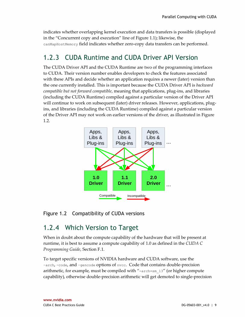
the one currently installed. This is important because the CUDA Driver API is backward
compatible but not forward compatible, meaning that applications, plug-ins, and libraries
(including the CUDA Runtime) compiled against a particular version of the Driver API
will continue to work on subsequent (later) driver releases. However, applications, plug-
ins, and libraries (including the CUDA Runtime) compiled against a particular version
of the Driver API may not work on earlier versions of the driver, as illustrated in Figure
1.2.
1.0
Driver
Apps,
Libs &
Plug-ins
1.1
Driver
Apps,
Libs &
Plug-ins
2.0
Driver
Apps,
Libs &
Plug-ins
Compatible Incompatible
...
...
Figure 1.2 Compatibility of CUDA versions
1.2.4 Which Version to Target
When in doubt about the compute capability of the hardware that will be present at
runtime, it is best to assume a compute capability of 1.0 as defined in the CUDA C
Programming Guide, Section F.1.
To target specific versions of NVIDIA hardware and CUDA software, use the
–arch, -code, and –gencode options of nvcc. Code that contains double-precision
arithmetic, for example, must be compiled with “-arch=sm_13” (or higher compute
capability), otherwise double-precision arithmetic will get demoted to single-precision
Parallel Computing with CUDA
www.nvidia.com
CUDA C Best Practices Guide DG-05603-001_v4.0 | 10
arithmetic (see Section 7.2.1). This and other compiler switches are discussed further in
Appendix B.
1.3 CUDA APIS
The host runtime component of the CUDA software environment can be used only by
host functions. It provides functions to handle the following:
Device management
Context management
Memory management
Code module management
Execution control
Texture reference management
Interoperability with OpenGL and Direct3D
It comprises two APIs:
A low-level API called the CUDA Driver API
A higher-level API called the CUDA Runtime API that is implemented on top of the
CUDA Driver API
Since version 3.1 of the CUDA software, these APIs are interoperable; applications can
do most operations in the more streamlined CUDA Runtime API while seamlessly
interoperating with the lower-level interfaces provided by the CUDA Driver API on an
as-needed basis.
Most commonly, applications will use the CUDA Runtime API, which greatly eases
device management by providing implicit initialization, context management, and
device code module management.
In contrast, while the CUDA Driver API offers more explicit control in certain limited
circumstances, it requires more code and is somewhat harder to program. For example,
it is more difficult to configure and launch kernels using the CUDA Driver API, since the
execution configuration and kernel parameters must be specified with explicit function
calls instead of the execution configuration syntax (<<<…>>>).
The C/C++ host code generated by nvcc utilizes the CUDA Runtime, so applications that
link to this code will depend on the CUDA Runtime; similarly, any code that uses the
CUBLAS, CUFFT, and other CUDA Toolkit libraries will also depend on the CUDA
Runtime, which is used internally by these libraries.
The two APIs can be easily distinguished: the CUDA Driver API is delivered through
the nvcuda/libcuda dynamic library and all its entry points are prefixed with cu; while
Parallel Computing with CUDA
www.nvidia.com
CUDA C Best Practices Guide DG-05603-001_v4.0 | 11
the CUDA Runtime is delivered through the cudart dynamic library and all its entry
points are prefixed with cuda. Note that the APIs relate only to host code; the kernels
that are executed on the device are the same, regardless of which API is used.
The functions that make up these two APIs are explained in the CUDA Reference Manual.
1.3.1 CUDA Runtime API
The CUDA Runtime handles kernel loading and setting up kernel parameters and
launch configuration before the kernel is launched. The implicit code initialization,
CUDA context management, CUDA module management (cubin to function mapping),
kernel configuration, and parameter passing are all performed by the CUDA Runtime.
It comprises two principal parts:
A C-style function interface (cuda_runtime_api.h).
C++-style convenience wrappers (cuda_runtime.h) built on top of the C-style
functions.
For more information on the Runtime API, refer to Section 3.2 of the CUDA C
Programming Guide.
1.3.2 CUDA Driver API
The Driver API is a lower-level API than the Runtime API. The Driver API has these
advantages:
More control over device contexts
No C extensions in the host code, so the host code can be compiled with compilers
other than nvcc and the host compiler it calls by default
Its primary disadvantages are as follows:
Much more verbose code
Linking against the CUDA Driver library requires additional application complexity,
since the driver may or may not be installed on a given target machine
Requires explicit management of device contexts and device code modules
For more information on the Driver API, refer to Section 3.3 of the CUDA C Programming
Guide.
1.3.3 When to Use Which API
The previous section lists some of the salient differences between the two APIs. A key
point is that for every Runtime API function, there is an equivalent Driver API function.
The Driver API does include a few functions omitted from the Runtime API, such as
Parallel Computing with CUDA
www.nvidia.com
CUDA C Best Practices Guide DG-05603-001_v4.0 | 12
functions for the explicit management of CUDA contexts, but most applications will not
need these additional functions (and, when they do, driver/runtime interoperability
allows the selective use of these functions on an as-needed basis), so use of the Runtime
API for most purposes is generally preferred.
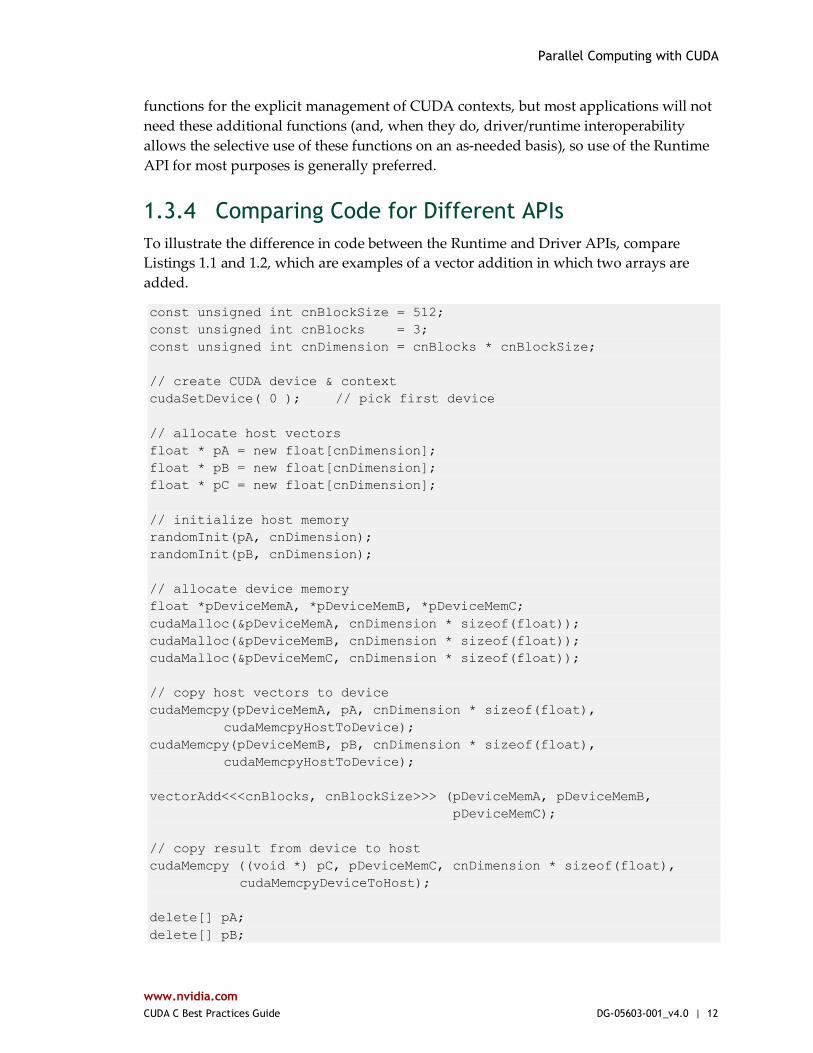
1.3.4 Comparing Code for Different APIs
To illustrate the difference in code between the Runtime and Driver APIs, compare
Listings 1.1 and 1.2, which are examples of a vector addition in which two arrays are
added.
const unsigned int cnBlockSize = 512;
const unsigned int cnBlocks = 3;
const unsigned int cnDimension = cnBlocks * cnBlockSize;
// create CUDA device & context
cudaSetDevice( 0 ); // pick first device
// allocate host vectors
float * pA = new float[cnDimension];
float * pB = new float[cnDimension];
float * pC = new float[cnDimension];
// initialize host memory
randomInit(pA, cnDimension);
randomInit(pB, cnDimension);
// allocate device memory
float *pDeviceMemA, *pDeviceMemB, *pDeviceMemC;
cudaMalloc(&pDeviceMemA, cnDimension * sizeof(float));
cudaMalloc(&pDeviceMemB, cnDimension * sizeof(float));
cudaMalloc(&pDeviceMemC, cnDimension * sizeof(float));
// copy host vectors to device
cudaMemcpy(pDeviceMemA, pA, cnDimension * sizeof(float),
cudaMemcpyHostToDevice);
cudaMemcpy(pDeviceMemB, pB, cnDimension * sizeof(float),
cudaMemcpyHostToDevice);
vectorAdd<<<cnBlocks, cnBlockSize>>> (pDeviceMemA, pDeviceMemB,
pDeviceMemC);
// copy result from device to host
cudaMemcpy ((void *) pC, pDeviceMemC, cnDimension * sizeof(float),
cudaMemcpyDeviceToHost);
delete[] pA;
delete[] pB;
Parallel Computing with CUDA
www.nvidia.com
CUDA C Best Practices Guide DG-05603-001_v4.0 | 13
delete[] pC;
cudaFree(pDeviceMemA);
cudaFree(pDeviceMemB);
cudaFree(pDeviceMemC);
Listing 1.1 Host code for adding two vectors using the CUDA Runtime
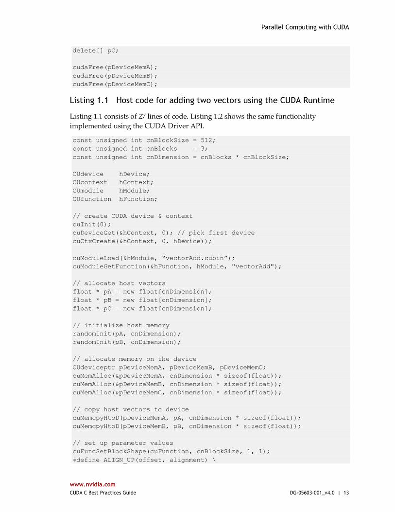
Listing 1.1 consists of 27 lines of code. Listing 1.2 shows the same functionality
implemented using the CUDA Driver API.
const unsigned int cnBlockSize = 512;
const unsigned int cnBlocks = 3;
const unsigned int cnDimension = cnBlocks * cnBlockSize;
CUdevice hDevice;
CUcontext hContext;
CUmodule hModule;
CUfunction hFunction;
// create CUDA device & context
cuInit(0);
cuDeviceGet(&hContext, 0); // pick first device
cuCtxCreate(&hContext, 0, hDevice));
cuModuleLoad(&hModule, “vectorAdd.cubin”);
cuModuleGetFunction(&hFunction, hModule, "vectorAdd");
// allocate host vectors
float * pA = new float[cnDimension];
float * pB = new float[cnDimension];
float * pC = new float[cnDimension];
// initialize host memory
randomInit(pA, cnDimension);
randomInit(pB, cnDimension);
// allocate memory on the device
CUdeviceptr pDeviceMemA, pDeviceMemB, pDeviceMemC;
cuMemAlloc(&pDeviceMemA, cnDimension * sizeof(float));
cuMemAlloc(&pDeviceMemB, cnDimension * sizeof(float));
cuMemAlloc(&pDeviceMemC, cnDimension * sizeof(float));
// copy host vectors to device
cuMemcpyHtoD(pDeviceMemA, pA, cnDimension * sizeof(float));
cuMemcpyHtoD(pDeviceMemB, pB, cnDimension * sizeof(float));
// set up parameter values
cuFuncSetBlockShape(cuFunction, cnBlockSize, 1, 1);
#define ALIGN_UP(offset, alignment) \
Parallel Computing with CUDA
www.nvidia.com
CUDA C Best Practices Guide DG-05603-001_v4.0 | 14
(offset) = ((offset) + (alignment) – 1) & ~((alignment) – 1)
int offset = 0;
ALIGN_UP(offset, __alignof(pDeviceMemA));
cuParamSetv(cuFunction, offset, &ptr, sizeof(pDeviceMemA));
offset += sizeof(pDeviceMemA);
ALIGN_UP(offset, __alignof(pDeviceMemB));
cuParamSetv(cuFunction, offset, &ptr, sizeof(pDeviceMemB));
offset += sizeof(pDeviceMemB);
ALIGN_UP(offset, __alignof(pDeviceMemC));
cuParamSetv(cuFunction, offset, &ptr, sizeof(pDeviceMemC));
offset += sizeof(pDeviceMemC);
cuParamSetSize(cuFunction, offset);
// execute kernel
cuLaunchGrid(cuFunction, cnBlocks, 1);
// copy the result from device back to host
cuMemcpyDtoH((void *) pC, pDeviceMemC,
cnDimension * sizeof(float));
delete[] pA;
delete[] pB;
delete[] pC;
cuMemFree(pDeviceMemA);
cuMemFree(pDeviceMemB);
cuMemFree(pDeviceMemC);
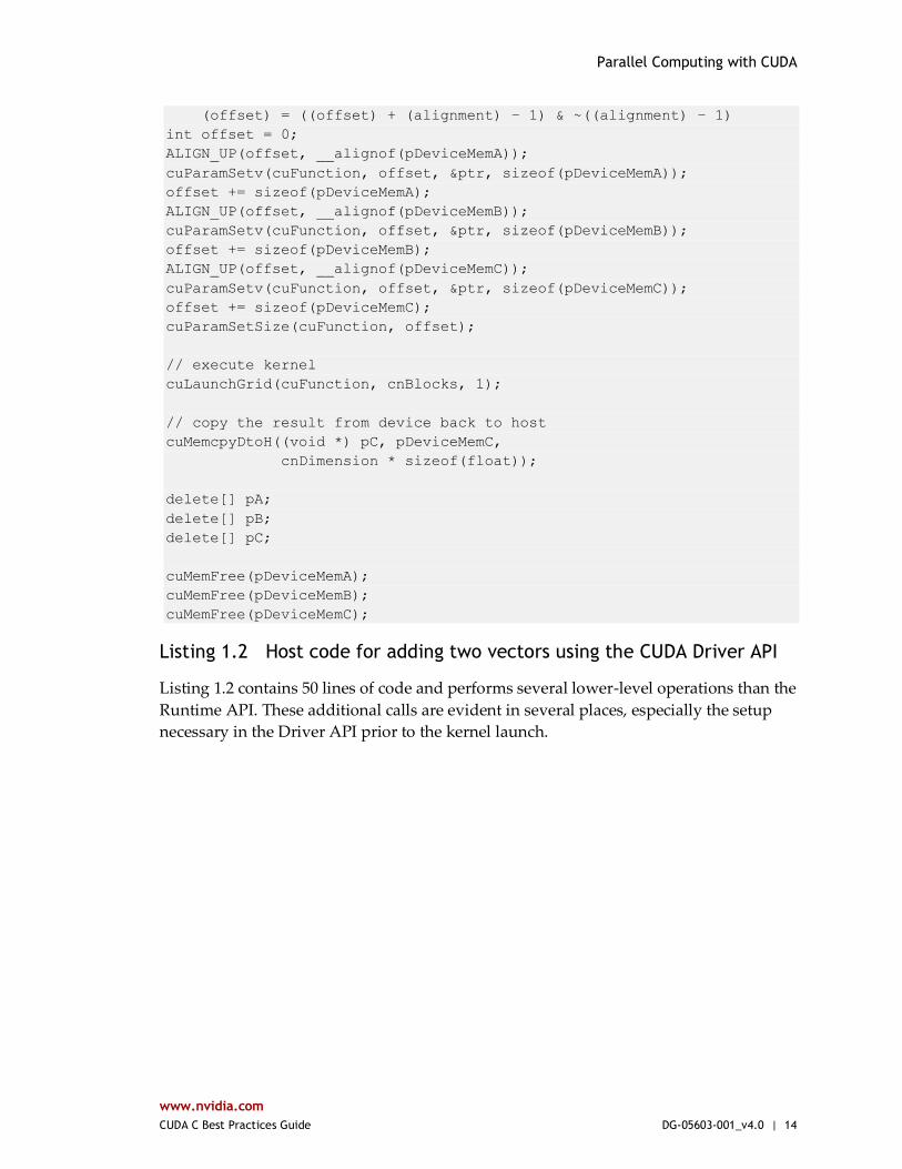
Listing 1.2 Host code for adding two vectors using the CUDA Driver API
Listing 1.2 contains 50 lines of code and performs several lower-level operations than the
Runtime API. These additional calls are evident in several places, especially the setup
necessary in the Driver API prior to the kernel launch.
www.nvidia.com
CUDA C Best Practices Guide DG-05603-001_v4.0 | 15
Chapter 2. PERFORMANCE METRICS
When attempting to optimize CUDA code, it pays to know how to measure performance
accurately and to understand the role that bandwidth plays in performance
measurement. This chapter discusses how to correctly measure performance using CPU
timers and CUDA events. It then explores how bandwidth affects performance metrics
and how to mitigate some of the challenges it poses.
2.1 TIMING
CUDA calls and kernel executions can be timed using either CPU or GPU timers. This
section examines the functionality, advantages, and pitfalls of both approaches.
2.1.1 Using CPU Timers
Any CPU timer can be used to measure the elapsed time of a CUDA call or kernel
execution. The details of various CPU timing approaches are outside the scope of this
document, but developers should always be aware of the resolution their timing calls
provide.
When using CPU timers, it is critical to remember that many CUDA API functions are
asynchronous; that is, they return control back to the calling CPU thread prior to
completing their work. All kernel launches are asynchronous, as are memory-copy
functions with the Async suffix on their names. Therefore, to accurately measure the
elapsed time for a particular call or sequence of CUDA calls, it is necessary to
synchronize the CPU thread with the GPU by calling cudaThreadSynchronize()
immediately before starting and stopping the CPU timer.
Performance Metrics
www.nvidia.com
CUDA C Best Practices Guide DG-05603-001_v4.0 | 16
cudaThreadSynchronize()blocks the calling CPU thread until all CUDA calls previously
issued by the thread are completed.
Although it is also possible to synchronize the CPU thread with a particular stream or
event on the GPU, these synchronization functions are not suitable for timing code in
streams other than the default stream. cudaStreamSynchronize() blocks the CPU thread
until all CUDA calls previously issued into the given stream have completed.
cudaEventSynchronize() blocks until a given event in a particular stream has been
recorded by the GPU. Because the driver may interleave execution of CUDA calls from
other non-default streams, calls in other streams may be included in the timing.
Because the default stream, stream 0, exhibits synchronous behavior (an operation in the
default stream can begin only after all preceding calls in any stream have completed;
and no subsequent operation in any stream can begin until it finishes), these functions
can be used reliably for timing in the default stream.
Be aware that CPU-to-GPU synchronization points such as those mentioned in this
section imply a stall in the GPU’s processing pipeline and should thus be used sparingly
to minimize their performance impact.
2.1.2 Using CUDA GPU Timers
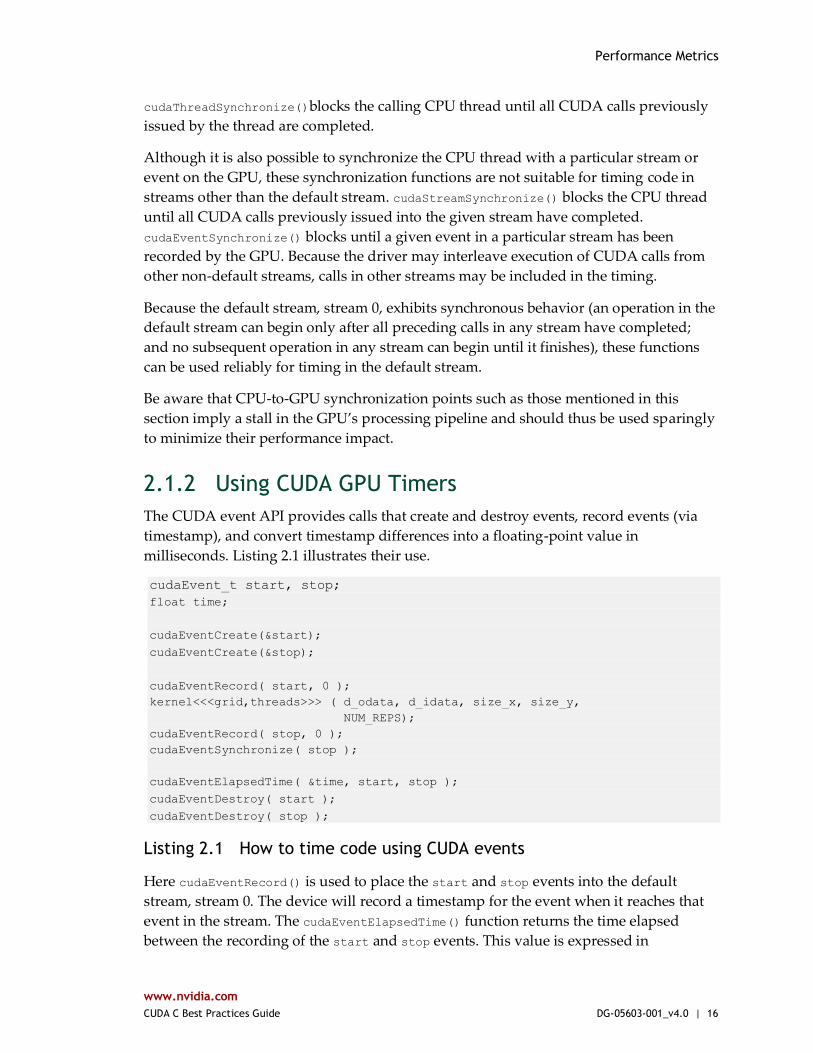
The CUDA event API provides calls that create and destroy events, record events (via
timestamp), and convert timestamp differences into a floating-point value in
milliseconds. Listing 2.1 illustrates their use.
cudaEvent_t start, stop;
float time;
cudaEventCreate(&start);
cudaEventCreate(&stop);
cudaEventRecord( start, 0 );
kernel<<<grid,threads>>> ( d_odata, d_idata, size_x, size_y,
NUM_REPS);
cudaEventRecord( stop, 0 );
cudaEventSynchronize( stop );
cudaEventElapsedTime( &time, start, stop );
cudaEventDestroy( start );
cudaEventDestroy( stop );
Listing 2.1 How to time code using CUDA events
Here cudaEventRecord() is used to place the start and stop events into the default
stream, stream 0. The device will record a timestamp for the event when it reaches that
event in the stream. The cudaEventElapsedTime() function returns the time elapsed
between the recording of the start and stop events. This value is expressed in
Performance Metrics
www.nvidia.com
CUDA C Best Practices Guide DG-05603-001_v4.0 | 17
milliseconds and has a resolution of approximately half a microsecond. Like the other
calls in this listing, their specific operation, parameters, and return values are described
in the CUDA Reference Manual. Note that the timings are measured on the GPU clock, so
the timing resolution is operating-system-independent.
2.2 BANDWIDTH
Bandwidth—the rate at which data can be transferred—is one of the most important
gating factors for performance. Almost all changes to code should be made in the
context of how they affect bandwidth. As described in Chapter 3 of this guide,
bandwidth can be dramatically affected by the choice of memory in which data is stored,
how the data is laid out and the order in which it is accessed, as well as other factors.
To measure performance accurately, it is useful to calculate theoretical and effective
bandwidth. When the latter is much lower than the former, design or implementation
details are likely to reduce bandwidth, and it should be the primary goal of subsequent
optimization efforts to increase it.
High Priority: Use the effective bandwidth of your computation as a metric when measuring performance and optimization benefits.
2.2.1 Theoretical Bandwidth Calculation
Theoretical bandwidth can be calculated using hardware specifications available in the
product literature. For example, the NVIDIA GeForce GTX 280 uses DDR (double data
rate) RAM with a memory clock rate of 1,107 MHz and a 512-bit wide memory interface.
Using these data items, the peak theoretical memory bandwidth of the NVIDIA GeForce
GTX 280 is 141.6 GB/sec:
( 1107 x 106 x ( 512/8 ) x 2 ) / 109 = 141.6 GB/sec
In this calculation, the memory clock rate is converted in to Hz, multiplied by the
interface width (divided by 8, to convert bits to bytes) and multiplied by 2 due to the
double data rate. Finally, this product is divided by 109 to convert the result to GB/sec
(GBps).
Note that some calculations use 1,0243 instead of 109 for the final calculation. In such a
case, the bandwidth would be 131.9 GBps. It is important to use the same divisor when
calculating theoretical and effective bandwidth so that the comparison is valid.
Performance Metrics
www.nvidia.com
CUDA C Best Practices Guide DG-05603-001_v4.0 | 18
2.2.2 Effective Bandwidth Calculation
Effective bandwidth is calculated by timing specific program activities and by knowing
how data is accessed by the program. To do so, use this equation:
Effective bandwidth = (( Br + Bw ) / 109 ) / time
Here, the effective bandwidth is in units of GBps, Br is the number of bytes read per
kernel, Bw is the number of bytes written per kernel, and time is given in seconds.
For example, to compute the effective bandwidth of a 2048 x 2048 matrix copy, the
following formula could be used:
Effective bandwidth = (( 20482 x 4 x 2 ) / 109 ) / time
The number of elements is multiplied by the size of each element (4 bytes for a float),
multiplied by 2 (because of the read and write), divided by 109 (or 1,0243) to obtain GB of
memory transferred. This number is divided by the time in seconds to obtain GBps.
2.2.3 Throughput Reported by cudaprof
The memory throughput reported in the summary table of cudaprof, the CUDA Visual
Profiler, differs from the effective bandwidth obtained by the calculation in Section 2.2.2
in several respects.
The first difference is that cudaprof measures throughput using a subset of the GPU’s
multiprocessors and then extrapolates that number to the entire GPU, thus reporting an
estimate of the data throughput.
The second and more important difference is that because the minimum memory
transaction size is larger than most word sizes, the memory throughput reported by the
profiler includes the transfer of data not used by the kernel.
The effective bandwidth calculation in Section 2.2.2, however, includes only data
transfers that are relevant to the algorithm. As such, the effective bandwidth will be
smaller than the memory throughput reported by cudaprof and is the number to use
when optimizing memory performance.
However, it’s important to note that both numbers are useful. The profiler memory
throughput shows how close the code is to the hardware limit, and the comparison of
the effective bandwidth with the profiler number presents a good estimate of how much
bandwidth is wasted by suboptimal coalescing of memory accesses.
www.nvidia.com
CUDA C Best Practices Guide DG-05603-001_v4.0 | 19
Chapter 3. MEMORY OPTIMIZATIONS
Memory optimizations are the most important area for performance. The goal is to
maximize the use of the hardware by maximizing bandwidth. Bandwidth is best served
by using as much fast memory and as little slow-access memory as possible. This
chapter discusses the various kinds of memory on the host and device and how best to
set up data items to use the memory effectively.
3.1 DATA TRANSFER BETWEEN HOST AND DEVICE
The peak bandwidth between the device memory and the GPU is much higher
(141 GBps on the NVIDIA GeForce GTX 280, for example) than the peak bandwidth
between host memory and device memory (8 GBps on the PCIe ×16 Gen2). Hence, for
best overall application performance, it is important to minimize data transfer between
the host and the device, even if that means running kernels on the GPU that do not
demonstrate any speed-up compared with running them on the host CPU.
High Priority: Minimize data transfer between the host and the device, even if it means running some kernels on the device that do not show performance gains when compared with running them on the host CPU.
Intermediate data structures should be created in device memory, operated on by the
device, and destroyed without ever being mapped by the host or copied to host
memory.
Also, because of the overhead associated with each transfer, batching many small
transfers into one larger transfer performs significantly better than making each transfer
separately.
Memory Optimizations
www.nvidia.com
CUDA C Best Practices Guide DG-05603-001_v4.0 | 20
Finally, higher bandwidth between the host and the device is achieved when using page-
locked (or pinned) memory, as discussed in the CUDA C Programming Guide and Section
3.1.1 of this document.
3.1.1 Pinned Memory
Page-locked or pinned memory transfers attain the highest bandwidth between the host
and the device. On PCIe ×16 Gen2 cards, for example, pinned memory can attain greater
than 5 GBps transfer rates.
Pinned memory is allocated using the cudaMallocHost()or cudaHostAlloc() functions in
the Runtime API. The bandwidthTest.cu program in the CUDA SDK shows how to use
these functions as well as how to measure memory transfer performance.
Pinned memory should not be overused. Excessive use can reduce overall system
performance because pinned memory is a scarce resource. How much is too much is
difficult to tell in advance, so as with all optimizations, test the applications and the
systems they run on for optimal performance parameters.
3.1.2 Asynchronous Transfers and Overlapping Transfers with Computation
Data transfers between the host and the device using cudaMemcpy() are blocking
transfers; that is, control is returned to the host thread only after the data transfer is
complete. The cudaMemcpyAsync() function is a non-blocking variant of cudaMemcpy() in
which control is returned immediately to the host thread. In contrast with cudaMemcpy(),
the asynchronous transfer version requires pinned host memory (see Section 3.1.1), and it
contains an additional argument, a stream ID. A stream is simply a sequence of
operations that are performed in order on the device. Operations in different streams
can be interleaved and in some cases overlapped—a property that can be used to hide
data transfers between the host and the device.
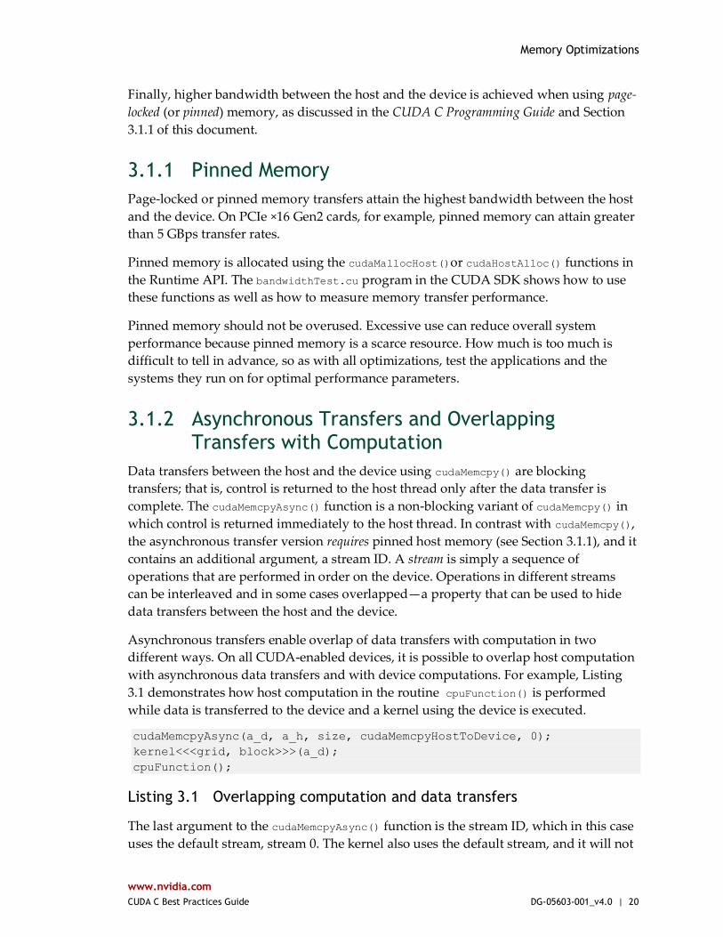
Asynchronous transfers enable overlap of data transfers with computation in two
different ways. On all CUDA-enabled devices, it is possible to overlap host computation
with asynchronous data transfers and with device computations. For example, Listing
3.1 demonstrates how host computation in the routine cpuFunction() is performed
while data is transferred to the device and a kernel using the device is executed.
cudaMemcpyAsync(a_d, a_h, size, cudaMemcpyHostToDevice, 0);
kernel<<<grid, block>>>(a_d);
cpuFunction();
Listing 3.1 Overlapping computation and data transfers
The last argument to the cudaMemcpyAsync() function is the stream ID, which in this case
uses the default stream, stream 0. The kernel also uses the default stream, and it will not
Memory Optimizations
www.nvidia.com
CUDA C Best Practices Guide DG-05603-001_v4.0 | 21
begin execution until the memory copy completes; therefore, no explicit synchronization
is needed. Because the memory copy and the kernel both return control to the host
immediately, the host function cpuFunction() overlaps their execution.
In Listing 3.1, the memory copy and kernel execution occur sequentially. On devices that
are capable of “concurrent copy and execute,” it is possible to overlap kernel execution
on the device with data transfers between the host and the device. Whether a device has
this capability is indicated by the deviceOverlap field of a cudaDeviceProp variable (or
listed in the output of the deviceQuery SDK sample). On devices that have this
capability, the overlap once again requires pinned host memory, and, in addition, the
data transfer and kernel must use different, non-default streams (streams with non-zero
stream IDs). Non-default streams are required for this overlap because memory copy,
memory set functions, and kernel calls that use the default stream begin only after all
preceding calls on the device (in any stream) have completed, and no operation on the
device (in any stream) commences until they are finished.
Listing 3.2 illustrates the basic technique.
cudaStreamCreate(&stream1);
cudaStreamCreate(&stream2);
cudaMemcpyAsync(a_d, a_h, size, cudaMemcpyHostToDevice, stream1);
kernel<<<grid, block, 0, stream2>>>(otherData_d);
Listing 3.2 Concurrent copy and execute
In this code, two streams are created and used in the data transfer and kernel executions
as specified in the last arguments of the cudaMemcpyAsync call and the kernel’s execution
configuration.
Listing 3.2 demonstrates how to overlap kernel execution with asynchronous data
transfer. This technique could be used when the data dependency is such that the data
can be broken into chunks and transferred in multiple stages, launching multiple kernels
to operate on each chunk as it arrives. Listings 3.3a and 3.3b demonstrate this. They
produce equivalent results. The first segment shows the reference sequential
implementation, which transfers and operates on an array of N floats (where N is
assumed to be evenly divisible by nThreads).
cudaMemcpy(a_d, a_h, N*sizeof(float), dir);
kernel<<<N/nThreads, nThreads>>>(a_d);
Listing 3.3a Sequential copy and execute
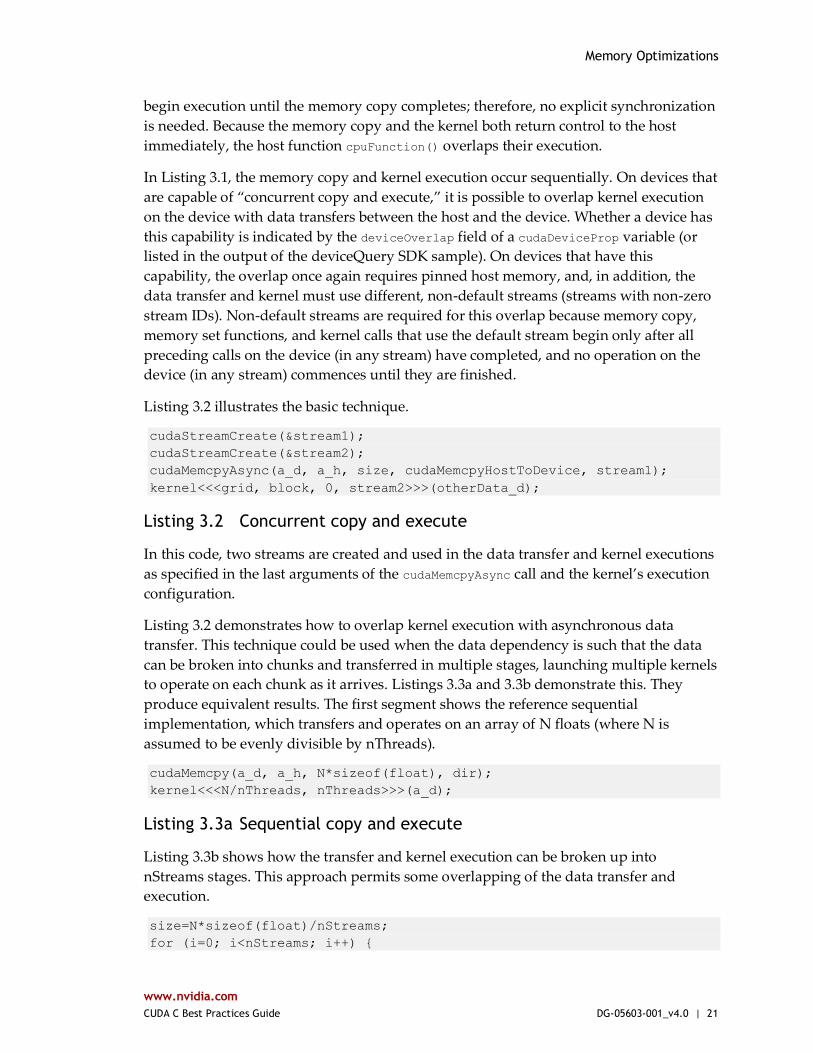
Listing 3.3b shows how the transfer and kernel execution can be broken up into
nStreams stages. This approach permits some overlapping of the data transfer and
execution.
size=N*sizeof(float)/nStreams;
for (i=0; i<nStreams; i++) {
Memory Optimizations
www.nvidia.com
CUDA C Best Practices Guide DG-05603-001_v4.0 | 22
offset = i*N/nStreams;
cudaMemcpyAsync(a_d+offset, a_h+offset, size, dir, stream[i]);
}
for (i=0; i<nStreams; i++) {
offset = i*N/nStreams;
kernel<<<N/(nThreads*nStreams), nThreads,
0, stream[i]>>>(a_d+offset);
}
Listing 3.3b Staged concurrent copy and execute
(In Listing 3.3b, it is assumed that N is evenly divisible by nThreads*nStreams.) Because
execution within a stream occurs sequentially, none of the kernels will launch until the
data transfers in their respective streams complete. Current hardware can
simultaneously process an asynchronous data transfer and execute kernels. (It should be
mentioned that it is not possible to overlap a blocking transfer with an asynchronous
transfer, because the blocking transfer occurs in the default stream, and so it will not
begin until all previous CUDA calls complete. It will not allow any other CUDA call to
begin until it has completed.) A diagram depicting the timeline of execution for the two
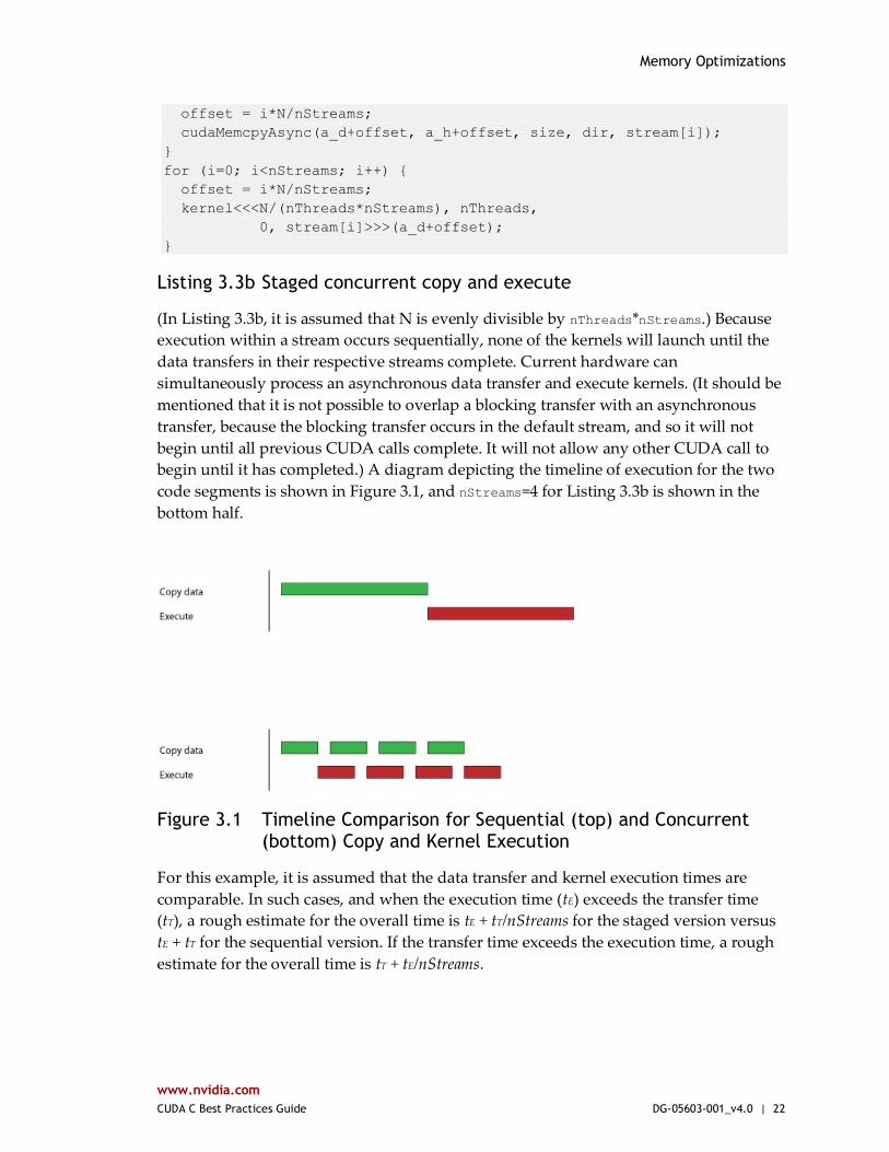
code segments is shown in Figure 3.1, and nStreams=4 for Listing 3.3b is shown in the
bottom half.
Figure 3.1 Timeline Comparison for Sequential (top) and Concurrent (bottom) Copy and Kernel Execution
For this example, it is assumed that the data transfer and kernel execution times are
comparable. In such cases, and when the execution time (tE) exceeds the transfer time
(tT), a rough estimate for the overall time is tE + tT/nStreams for the staged version versus
tE + tT for the sequential version. If the transfer time exceeds the execution time, a rough
estimate for the overall time is tT + tE/nStreams.
Memory Optimizations
www.nvidia.com
CUDA C Best Practices Guide DG-05603-001_v4.0 | 23
3.1.3 Zero Copy
Zero copy is a feature that was added in version 2.2 of the CUDA Toolkit. It enables GPU
threads to directly access host memory. For this purpose, it requires mapped pinned
(non-pageable) memory. On integrated GPUs (e.g., mobile GPUs for notebooks),
mapped pinned memory is always a performance gain because it avoids superfluous
copies as integrated GPU and CPU memory are physically the same. On discrete GPUs,
mapped pinned memory is advantageous only in certain cases. Because the data is not
cached on the GPU on devices of compute capability 1.x, mapped pinned memory
should be read or written only once, and the global loads and stores that read and write
the memory should be coalesced. Zero copy can be used in place of streams because
kernel-originated data transfers automatically overlap kernel execution without the
overhead of setting up and determining the optimal number of streams.
Low Priority: Use zero-copy operations on integrated GPUs for CUDA Toolkit version 2.2 and later.
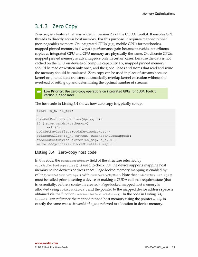
The host code in Listing 3.4 shows how zero copy is typically set up.
float *a_h, *a_map;
…
cudaGetDeviceProperties(&prop, 0);
if (!prop.canMapHostMemory)
exit(0);
cudaSetDeviceFlags(cudaDeviceMapHost);
cudaHostAlloc(&a_h, nBytes, cudaHostAllocMapped);
cudaHostGetDevicePointer(&a_map, a_h, 0);
kernel<<<gridSize, blockSize>>>(a_map);
Listing 3.4 Zero-copy host code
In this code, the canMapHostMemory field of the structure returned by
cudaGetDeviceProperties() is used to check that the device supports mapping host
memory to the device’s address space. Page-locked memory mapping is enabled by
calling cudaSetDeviceFlags() with cudaDeviceMapHost. Note that cudaSetDeviceFlags()
must be called prior to setting a device or making a CUDA call that requires state (that
is, essentially, before a context is created). Page-locked mapped host memory is
allocated using cudaHostAlloc(), and the pointer to the mapped device address space is
obtained via the function cudaHostGetDevicePointer(). In the code in Listing 3.4,
kernel() can reference the mapped pinned host memory using the pointer a_map in
exactly the same was as it would if a_map referred to a location in device memory.
Memory Optimizations
www.nvidia.com
CUDA C Best Practices Guide DG-05603-001_v4.0 | 24
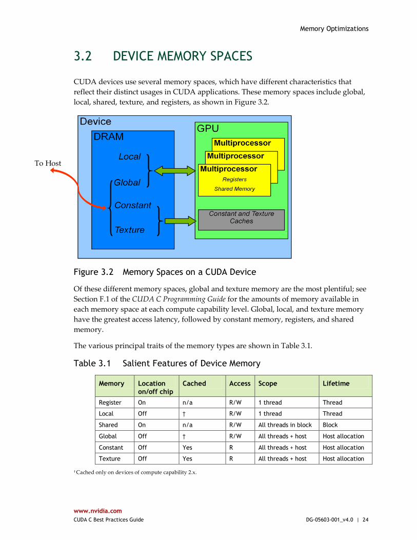
3.2 DEVICE MEMORY SPACES
CUDA devices use several memory spaces, which have different characteristics that
reflect their distinct usages in CUDA applications. These memory spaces include global,
local, shared, texture, and registers, as shown in Figure 3.2.
Figure 3.2 Memory Spaces on a CUDA Device
Of these different memory spaces, global and texture memory are the most plentiful; see
Section F.1 of the CUDA C Programming Guide for the amounts of memory available in
each memory space at each compute capability level. Global, local, and texture memory
have the greatest access latency, followed by constant memory, registers, and shared
memory.
The various principal traits of the memory types are shown in Table 3.1.
Table 3.1 Salient Features of Device Memory
Memory Location
on/off chip
Cached Access Scope Lifetime
Register On n/a R/W 1 thread Thread
Local Off † R/W 1 thread Thread
Shared On n/a R/W All threads in block Block
Global Off † R/W All threads + host Host allocation
Constant Off Yes R All threads + host Host allocation
Texture Off Yes R All threads + host Host allocation
† Cached only on devices of compute capability 2.x.
To Host
Memory Optimizations
www.nvidia.com
CUDA C Best Practices Guide DG-05603-001_v4.0 | 25
In the case of texture access, if a texture reference is bound to a linear (and, as of version
2.2 of the CUDA Toolkit, pitch-linear) array in global memory, then the device code can
write to the underlying array. Reading from a texture while writing to its underlying
global memory array in the same kernel launch should be avoided because the texture
caches are read-only and are not invalidated when the associated global memory is
modified.
3.2.1 Coalesced Access to Global Memory
High Priority: Ensure global memory accesses are coalesced whenever possible.
Perhaps the single most important performance consideration in programming for the
CUDA architecture is coalescing global memory accesses. Global memory loads and
stores by threads of a half warp (for devices of compute capability 1.x) or of a warp (for
devices of compute capability 2.x) are coalesced by the device into as few as one
transaction when certain access requirements are met.
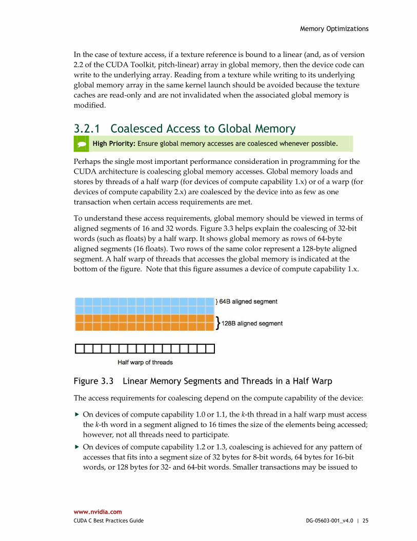
To understand these access requirements, global memory should be viewed in terms of
aligned segments of 16 and 32 words. Figure 3.3 helps explain the coalescing of 32-bit
words (such as floats) by a half warp. It shows global memory as rows of 64-byte
aligned segments (16 floats). Two rows of the same color represent a 128-byte aligned
segment. A half warp of threads that accesses the global memory is indicated at the
bottom of the figure. Note that this figure assumes a device of compute capability 1.x.
Figure 3.3 Linear Memory Segments and Threads in a Half Warp
The access requirements for coalescing depend on the compute capability of the device:
On devices of compute capability 1.0 or 1.1, the k-th thread in a half warp must access
the k-th word in a segment aligned to 16 times the size of the elements being accessed;
however, not all threads need to participate.
On devices of compute capability 1.2 or 1.3, coalescing is achieved for any pattern of
accesses that fits into a segment size of 32 bytes for 8-bit words, 64 bytes for 16-bit
words, or 128 bytes for 32- and 64-bit words. Smaller transactions may be issued to
Memory Optimizations
www.nvidia.com
CUDA C Best Practices Guide DG-05603-001_v4.0 | 26
avoid wasting bandwidth. More precisely, the following protocol is used to issue a
memory transaction for a half warp:
● Find the memory segment that contains the address requested by the lowest
numbered active thread. Segment size is 32 bytes for 8-bit data, 64 bytes for 16-bit
data, and 128 bytes for 32-, 64-, and 128-bit data.
● Find all other active threads whose requested address lies in the same segment,
and reduce the transaction size if possible:
― If the transaction is 128 bytes and only the lower or upper half is used, reduce
the transaction size to 64 bytes.
― If the transaction is 64 bytes and only the lower or upper half is used, reduce the
transaction size to 32 bytes.
● Carry out the transaction and mark the serviced threads as inactive.
● Repeat until all threads in the half warp are serviced.
● On devices of compute capability 2.x, memory accesses by the threads of a warp
are coalesced into the minimum number of L1-cache-line-sized aligned
transactions necessary to satisfy all threads; see Section F.4.2 of the CUDA C
Programming Guide.
These concepts are illustrated in the following simple examples.
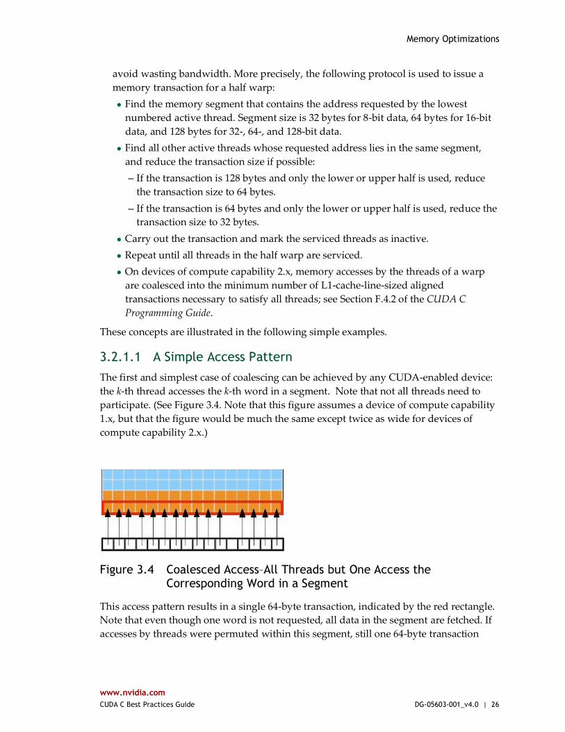
3.2.1.1 A Simple Access Pattern
The first and simplest case of coalescing can be achieved by any CUDA-enabled device:
the k-th thread accesses the k-th word in a segment. Note that not all threads need to
participate. (See Figure 3.4. Note that this figure assumes a device of compute capability
1.x, but that the figure would be much the same except twice as wide for devices of
compute capability 2.x.)
Figure 3.4 Coalesced Access–All Threads but One Access the Corresponding Word in a Segment
This access pattern results in a single 64-byte transaction, indicated by the red rectangle.
Note that even though one word is not requested, all data in the segment are fetched. If
accesses by threads were permuted within this segment, still one 64-byte transaction
Memory Optimizations
www.nvidia.com
CUDA C Best Practices Guide DG-05603-001_v4.0 | 27
would be performed by a device with compute capability 1.2 or higher, but 16 serialized
transactions would be performed by a device with compute capability 1.1 or lower.
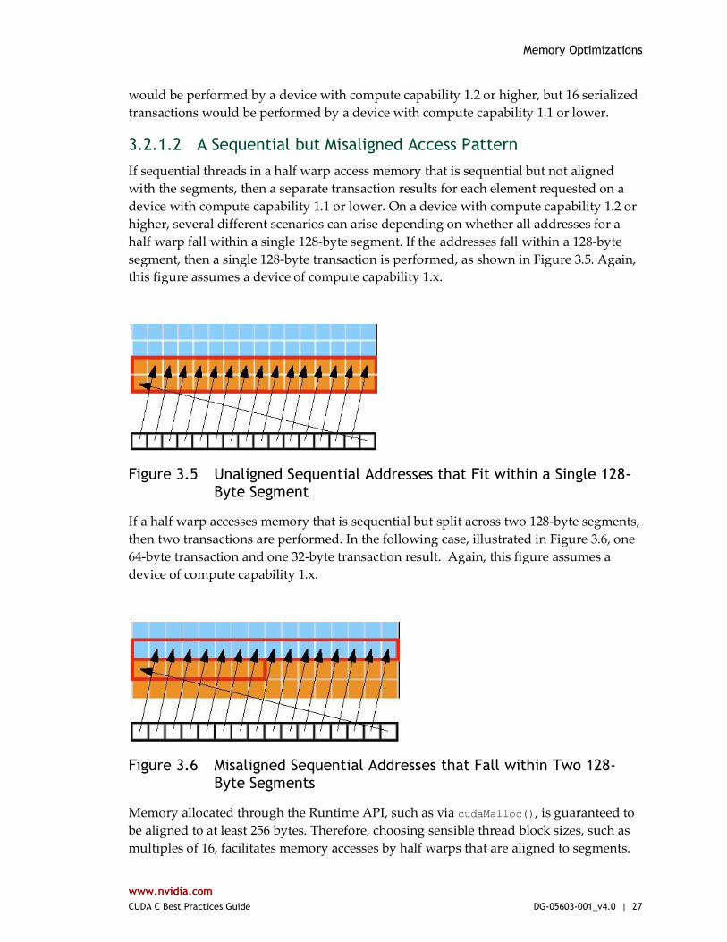
3.2.1.2 A Sequential but Misaligned Access Pattern
If sequential threads in a half warp access memory that is sequential but not aligned
with the segments, then a separate transaction results for each element requested on a
device with compute capability 1.1 or lower. On a device with compute capability 1.2 or
higher, several different scenarios can arise depending on whether all addresses for a
half warp fall within a single 128-byte segment. If the addresses fall within a 128-byte
segment, then a single 128-byte transaction is performed, as shown in Figure 3.5. Again,
this figure assumes a device of compute capability 1.x.
Figure 3.5 Unaligned Sequential Addresses that Fit within a Single 128-Byte Segment
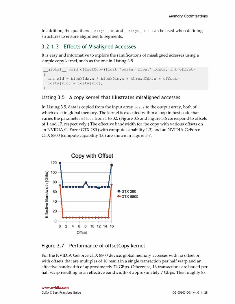
If a half warp accesses memory that is sequential but split across two 128-byte segments,
then two transactions are performed. In the following case, illustrated in Figure 3.6, one
64-byte transaction and one 32-byte transaction result. Again, this figure assumes a
device of compute capability 1.x.
Figure 3.6 Misaligned Sequential Addresses that Fall within Two 128-Byte Segments
Memory allocated through the Runtime API, such as via cudaMalloc(), is guaranteed to
be aligned to at least 256 bytes. Therefore, choosing sensible thread block sizes, such as
multiples of 16, facilitates memory accesses by half warps that are aligned to segments.
Memory Optimizations
www.nvidia.com
CUDA C Best Practices Guide DG-05603-001_v4.0 | 28
In addition, the qualifiers __align__(8) and __align__(16) can be used when defining
structures to ensure alignment to segments.
3.2.1.3 Effects of Misaligned Accesses
It is easy and informative to explore the ramifications of misaligned accesses using a
simple copy kernel, such as the one in Listing 3.5.
__global__ void offsetCopy(float *odata, float* idata, int offset)
{
int xid = blockIdx.x * blockDim.x + threadIdx.x + offset;
odata[xid] = idata[xid];
}
Listing 3.5 A copy kernel that illustrates misaligned accesses
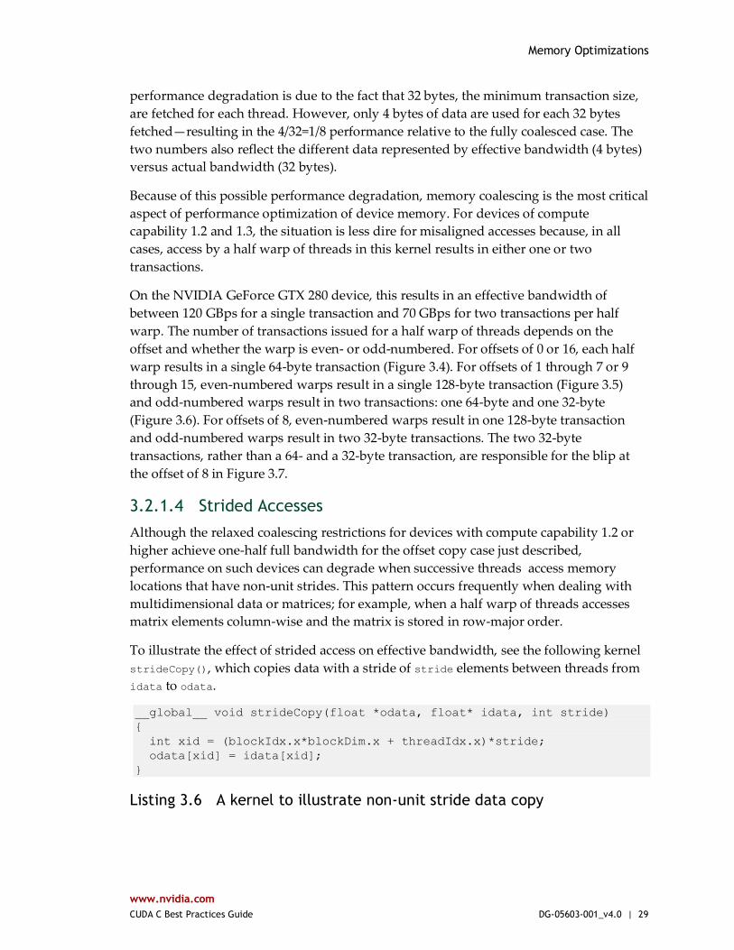
In Listing 3.5, data is copied from the input array idata to the output array, both of
which exist in global memory. The kernel is executed within a loop in host code that
varies the parameter offset from 1 to 32. (Figure 3.5 and Figure 3.6 correspond to offsets
of 1 and 17, respectively.) The effective bandwidth for the copy with various offsets on
an NVIDIA GeForce GTX 280 (with compute capability 1.3) and an NVIDIA GeForce
GTX 8800 (compute capability 1.0) are shown in Figure 3.7.
Figure 3.7 Performance of offsetCopy kernel
For the NVIDIA GeForce GTX 8800 device, global memory accesses with no offset or
with offsets that are multiples of 16 result in a single transaction per half warp and an
effective bandwidth of approximately 74 GBps. Otherwise, 16 transactions are issued per
half warp resulting in an effective bandwidth of approximately 7 GBps. This roughly 8x
Memory Optimizations
www.nvidia.com
CUDA C Best Practices Guide DG-05603-001_v4.0 | 29
performance degradation is due to the fact that 32 bytes, the minimum transaction size,
are fetched for each thread. However, only 4 bytes of data are used for each 32 bytes
fetched—resulting in the 4/32=1/8 performance relative to the fully coalesced case. The
two numbers also reflect the different data represented by effective bandwidth (4 bytes)
versus actual bandwidth (32 bytes).
Because of this possible performance degradation, memory coalescing is the most critical
aspect of performance optimization of device memory. For devices of compute
capability 1.2 and 1.3, the situation is less dire for misaligned accesses because, in all
cases, access by a half warp of threads in this kernel results in either one or two
transactions.
On the NVIDIA GeForce GTX 280 device, this results in an effective bandwidth of
between 120 GBps for a single transaction and 70 GBps for two transactions per half
warp. The number of transactions issued for a half warp of threads depends on the
offset and whether the warp is even- or odd-numbered. For offsets of 0 or 16, each half
warp results in a single 64-byte transaction (Figure 3.4). For offsets of 1 through 7 or 9
through 15, even-numbered warps result in a single 128-byte transaction (Figure 3.5)
and odd-numbered warps result in two transactions: one 64-byte and one 32-byte
(Figure 3.6). For offsets of 8, even-numbered warps result in one 128-byte transaction
and odd-numbered warps result in two 32-byte transactions. The two 32-byte
transactions, rather than a 64- and a 32-byte transaction, are responsible for the blip at
the offset of 8 in Figure 3.7.
3.2.1.4 Strided Accesses
Although the relaxed coalescing restrictions for devices with compute capability 1.2 or
higher achieve one-half full bandwidth for the offset copy case just described,
performance on such devices can degrade when successive threads access memory
locations that have non-unit strides. This pattern occurs frequently when dealing with
multidimensional data or matrices; for example, when a half warp of threads accesses
matrix elements column-wise and the matrix is stored in row-major order.
To illustrate the effect of strided access on effective bandwidth, see the following kernel
strideCopy(), which copies data with a stride of stride elements between threads from
idata to odata.
__global__ void strideCopy(float *odata, float* idata, int stride)
{
int xid = (blockIdx.x*blockDim.x + threadIdx.x)*stride;
odata[xid] = idata[xid];
}
Listing 3.6 A kernel to illustrate non-unit stride data copy
Memory Optimizations
www.nvidia.com
CUDA C Best Practices Guide DG-05603-001_v4.0 | 30
Figure 3.8 illustrates a situation that can be created using the code in Listing 3.6; namely,
threads within a half warp access memory with a stride of 2. This action is coalesced into
a single 128-byte transaction on an NVIDIA GeForce GTX 280 (compute capability 1.3).
Figure 3.8 A half warp accessing memory with a stride of 2
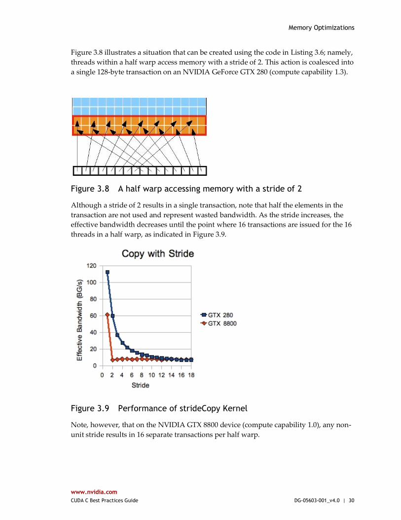
Although a stride of 2 results in a single transaction, note that half the elements in the
transaction are not used and represent wasted bandwidth. As the stride increases, the
effective bandwidth decreases until the point where 16 transactions are issued for the 16
threads in a half warp, as indicated in Figure 3.9.
Figure 3.9 Performance of strideCopy Kernel
Note, however, that on the NVIDIA GTX 8800 device (compute capability 1.0), any non-
unit stride results in 16 separate transactions per half warp.
Memory Optimizations
www.nvidia.com
CUDA C Best Practices Guide DG-05603-001_v4.0 | 31
As illustrated in Figure 3.9, non-unit stride global memory accesses should be avoided
whenever possible. One method for doing so utilizes shared memory, which is
discussed in the next section.
3.2.2 Shared Memory
Because it is on-chip, shared memory is much faster than local and global memory. In
fact, uncached shared memory latency is roughly 100x lower than global memory
latency—provided there are no bank conflicts between the threads, as detailed in the
following section.
3.2.2.1 Shared Memory and Memory Banks
To achieve high memory bandwidth for concurrent accesses, shared memory is divided
into equally sized memory modules (banks) that can be accessed simultaneously.
Therefore, any memory load or store of n addresses that spans n distinct memory banks
can be serviced simultaneously, yielding an effective bandwidth that is n times as high
as the bandwidth of a single bank.
However, if multiple addresses of a memory request map to the same memory bank, the
accesses are serialized. The hardware splits a memory request that has bank conflicts
into as many separate conflict-free requests as necessary, decreasing the effective
bandwidth by a factor equal to the number of separate memory requests. The one
exception here is when all threads in a half warp address the same shared memory
location, resulting in a broadcast. Devices of compute capability 2.x have the additional
ability to multicast shared memory accesses (i.e., to send copies of the same value to
several but not all threads of the warp).
To minimize bank conflicts, it is important to understand how memory addresses map
to memory banks and how to optimally schedule memory requests.
Medium Priority: Accesses to shared memory should be designed to avoid serializing requests due to bank conflicts.
Shared memory banks are organized such that successive 32-bit words are assigned to
successive banks and each bank has a bandwidth of 32 bits per clock cycle. The
bandwidth of shared memory is 32 bits per bank per clock cycle.
For devices of compute capability 1.x, the warp size is 32 threads and the number of
banks is 16. A shared memory request for a warp is split into one request for the first
half of the warp and one request for the second half of the warp. Note that no bank
conflict occurs if only one memory location per bank is accessed by a half warp of
threads.
For devices of compute capability 2.x, the warp size is 32 threads and the number of
banks is also 32. A shared memory request for a warp is not split as with devices of
Memory Optimizations
www.nvidia.com
CUDA C Best Practices Guide DG-05603-001_v4.0 | 32
compute capability 1.x, meaning that bank conflicts can occur between threads in the
first half of a warp and threads in the second half of the same warp (see Section F.4.3 of
the CUDA C Programming Guide).
Refer to the CUDA C Programming Guide for more information on how accesses and
banks can be matched to avoid conflicts.
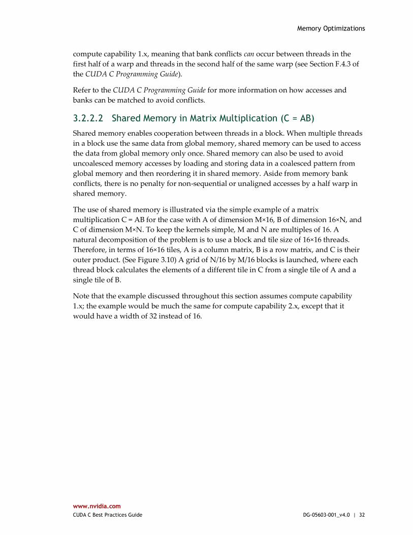
3.2.2.2 Shared Memory in Matrix Multiplication (C = AB)
Shared memory enables cooperation between threads in a block. When multiple threads
in a block use the same data from global memory, shared memory can be used to access
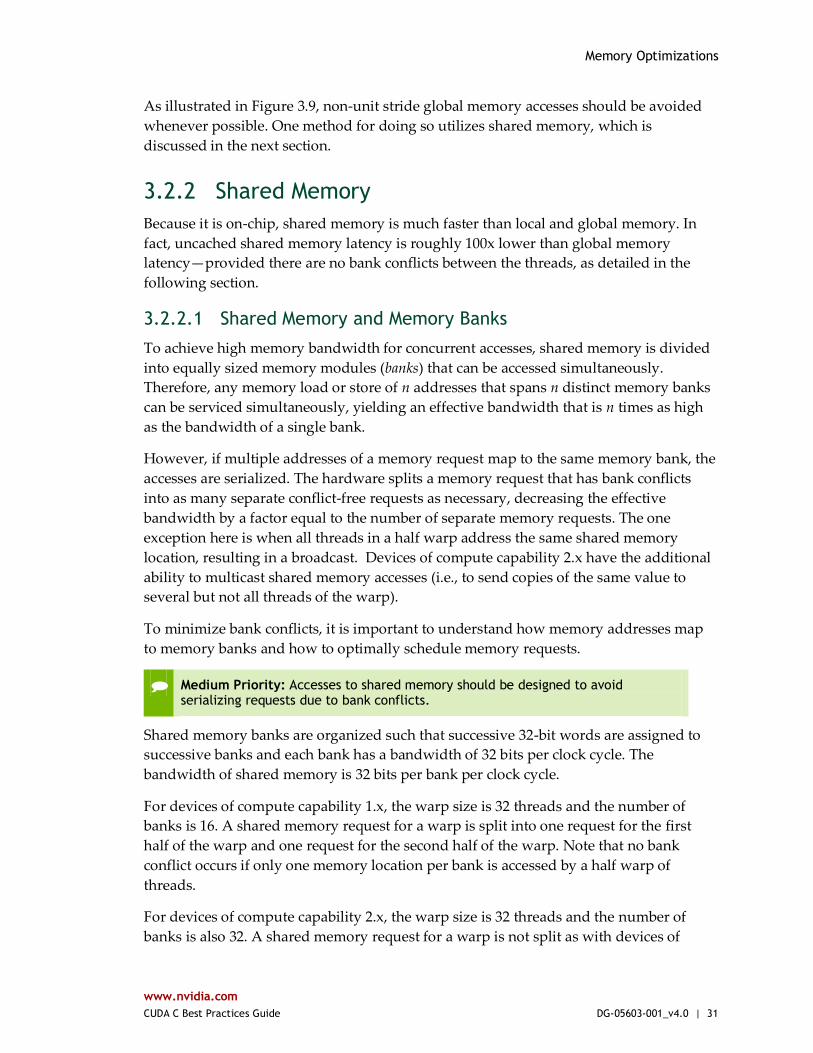
the data from global memory only once. Shared memory can also be used to avoid
uncoalesced memory accesses by loading and storing data in a coalesced pattern from
global memory and then reordering it in shared memory. Aside from memory bank
conflicts, there is no penalty for non-sequential or unaligned accesses by a half warp in
shared memory.
The use of shared memory is illustrated via the simple example of a matrix
multiplication C = AB for the case with A of dimension M×16, B of dimension 16×N, and
C of dimension M×N. To keep the kernels simple, M and N are multiples of 16. A
natural decomposition of the problem is to use a block and tile size of 16×16 threads.
Therefore, in terms of 16×16 tiles, A is a column matrix, B is a row matrix, and C is their
outer product. (See Figure 3.10) A grid of N/16 by M/16 blocks is launched, where each
thread block calculates the elements of a different tile in C from a single tile of A and a
single tile of B.
Note that the example discussed throughout this section assumes compute capability
1.x; the example would be much the same for compute capability 2.x, except that it
would have a width of 32 instead of 16.
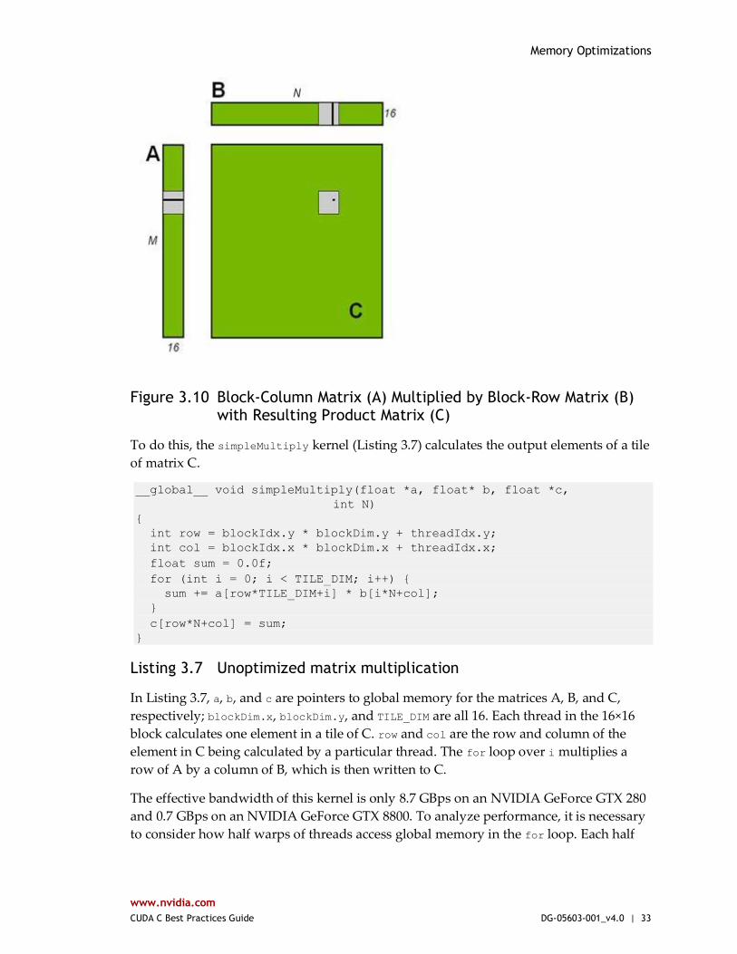
Memory Optimizations
www.nvidia.com
CUDA C Best Practices Guide DG-05603-001_v4.0 | 33
Figure 3.10 Block-Column Matrix (A) Multiplied by Block-Row Matrix (B) with Resulting Product Matrix (C)
To do this, the simpleMultiply kernel (Listing 3.7) calculates the output elements of a tile
of matrix C.
__global__ void simpleMultiply(float *a, float* b, float *c,
int N)
{
int row = blockIdx.y * blockDim.y + threadIdx.y;
int col = blockIdx.x * blockDim.x + threadIdx.x;
float sum = 0.0f;
for (int i = 0; i < TILE_DIM; i++) {
sum += a[row*TILE_DIM+i] * b[i*N+col];
}
c[row*N+col] = sum;
}
Listing 3.7 Unoptimized matrix multiplication
In Listing 3.7, a, b, and c are pointers to global memory for the matrices A, B, and C,
respectively; blockDim.x, blockDim.y, and TILE_DIM are all 16. Each thread in the 16×16
block calculates one element in a tile of C. row and col are the row and column of the
element in C being calculated by a particular thread. The for loop over i multiplies a
row of A by a column of B, which is then written to C.
The effective bandwidth of this kernel is only 8.7 GBps on an NVIDIA GeForce GTX 280
and 0.7 GBps on an NVIDIA GeForce GTX 8800. To analyze performance, it is necessary
to consider how half warps of threads access global memory in the for loop. Each half
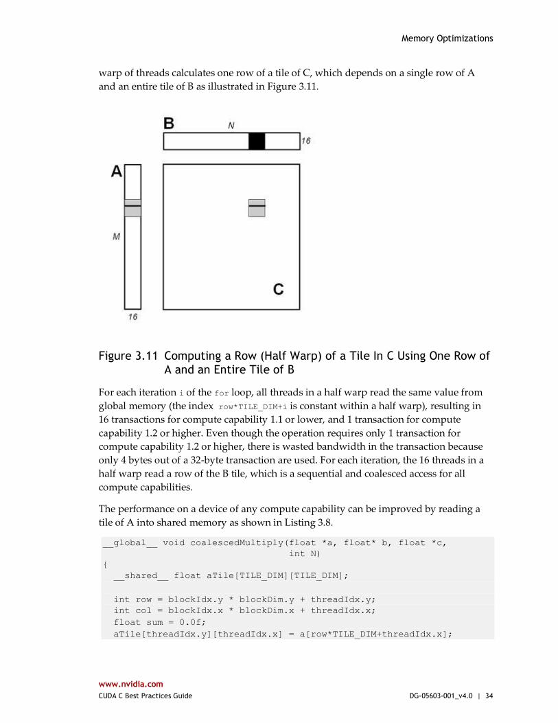
Memory Optimizations
www.nvidia.com
CUDA C Best Practices Guide DG-05603-001_v4.0 | 34
warp of threads calculates one row of a tile of C, which depends on a single row of A
and an entire tile of B as illustrated in Figure 3.11.
Figure 3.11 Computing a Row (Half Warp) of a Tile In C Using One Row of A and an Entire Tile of B
For each iteration i of the for loop, all threads in a half warp read the same value from
global memory (the index row*TILE_DIM+i is constant within a half warp), resulting in
16 transactions for compute capability 1.1 or lower, and 1 transaction for compute
capability 1.2 or higher. Even though the operation requires only 1 transaction for
compute capability 1.2 or higher, there is wasted bandwidth in the transaction because
only 4 bytes out of a 32-byte transaction are used. For each iteration, the 16 threads in a
half warp read a row of the B tile, which is a sequential and coalesced access for all
compute capabilities.
The performance on a device of any compute capability can be improved by reading a
tile of A into shared memory as shown in Listing 3.8.
__global__ void coalescedMultiply(float *a, float* b, float *c,
int N)
{
__shared__ float aTile[TILE_DIM][TILE_DIM];
int row = blockIdx.y * blockDim.y + threadIdx.y;
int col = blockIdx.x * blockDim.x + threadIdx.x;
float sum = 0.0f;
aTile[threadIdx.y][threadIdx.x] = a[row*TILE_DIM+threadIdx.x];
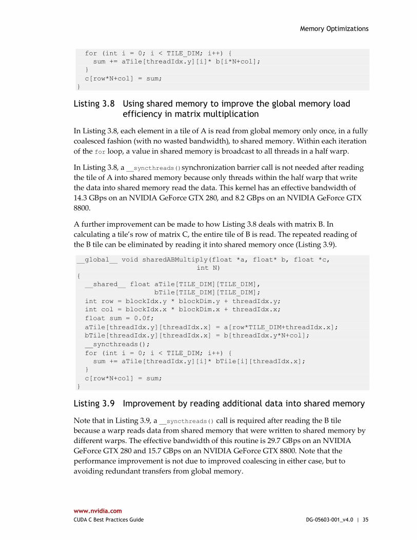
Memory Optimizations
www.nvidia.com
CUDA C Best Practices Guide DG-05603-001_v4.0 | 35
for (int i = 0; i < TILE_DIM; i++) {
sum += aTile[threadIdx.y][i]* b[i*N+col];
}
c[row*N+col] = sum;
}
Listing 3.8 Using shared memory to improve the global memory load efficiency in matrix multiplication
In Listing 3.8, each element in a tile of A is read from global memory only once, in a fully
coalesced fashion (with no wasted bandwidth), to shared memory. Within each iteration
of the for loop, a value in shared memory is broadcast to all threads in a half warp.
In Listing 3.8, a __syncthreads()synchronization barrier call is not needed after reading
the tile of A into shared memory because only threads within the half warp that write
the data into shared memory read the data. This kernel has an effective bandwidth of
14.3 GBps on an NVIDIA GeForce GTX 280, and 8.2 GBps on an NVIDIA GeForce GTX
8800.
A further improvement can be made to how Listing 3.8 deals with matrix B. In
calculating a tile’s row of matrix C, the entire tile of B is read. The repeated reading of
the B tile can be eliminated by reading it into shared memory once (Listing 3.9).
__global__ void sharedABMultiply(float *a, float* b, float *c,
int N)
{
__shared__ float aTile[TILE_DIM][TILE_DIM],
bTile[TILE_DIM][TILE_DIM];
int row = blockIdx.y * blockDim.y + threadIdx.y;
int col = blockIdx.x * blockDim.x + threadIdx.x;
float sum = 0.0f;
aTile[threadIdx.y][threadIdx.x] = a[row*TILE_DIM+threadIdx.x];
bTile[threadIdx.y][threadIdx.x] = b[threadIdx.y*N+col];
__syncthreads();
for (int i = 0; i < TILE_DIM; i++) {
sum += aTile[threadIdx.y][i]* bTile[i][threadIdx.x];
}
c[row*N+col] = sum;
}
Listing 3.9 Improvement by reading additional data into shared memory
Note that in Listing 3.9, a __syncthreads() call is required after reading the B tile
because a warp reads data from shared memory that were written to shared memory by
different warps. The effective bandwidth of this routine is 29.7 GBps on an NVIDIA
GeForce GTX 280 and 15.7 GBps on an NVIDIA GeForce GTX 8800. Note that the
performance improvement is not due to improved coalescing in either case, but to
avoiding redundant transfers from global memory.
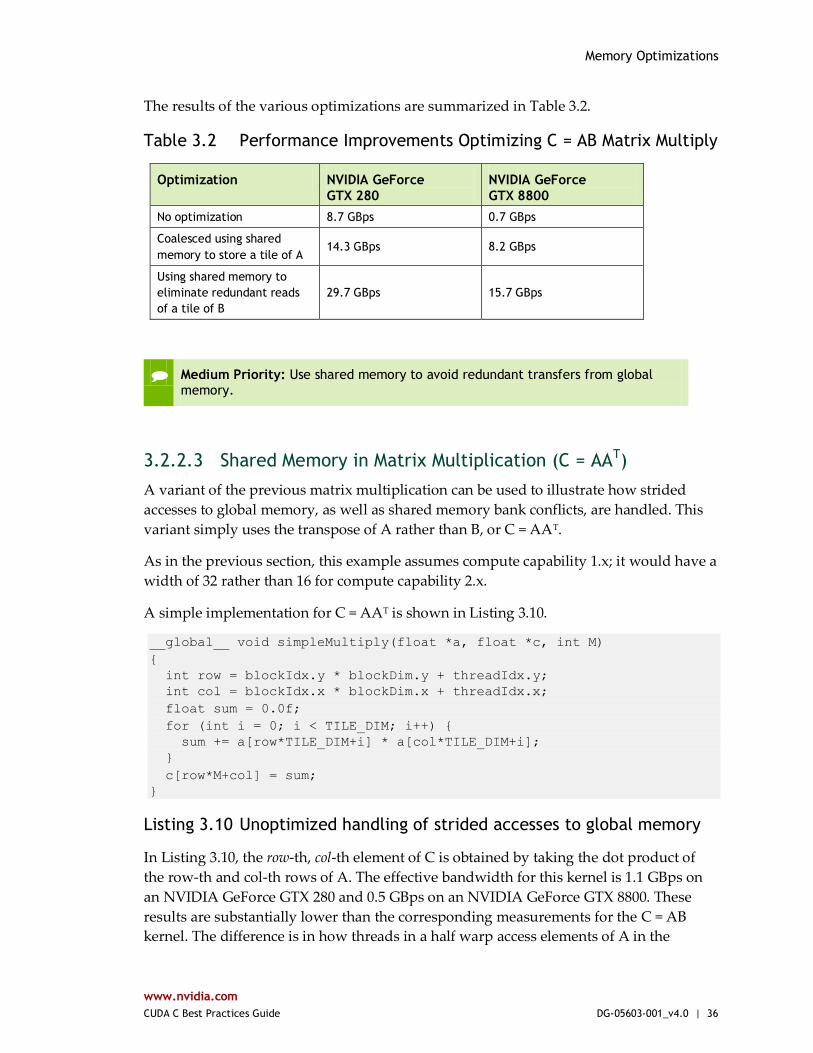
Memory Optimizations
www.nvidia.com
CUDA C Best Practices Guide DG-05603-001_v4.0 | 36
The results of the various optimizations are summarized in Table 3.2.
Table 3.2 Performance Improvements Optimizing C = AB Matrix Multiply
Optimization NVIDIA GeForce
GTX 280
NVIDIA GeForce
GTX 8800
No optimization 8.7 GBps 0.7 GBps
Coalesced using shared
memory to store a tile of A 14.3 GBps 8.2 GBps
Using shared memory to
eliminate redundant reads
of a tile of B
29.7 GBps 15.7 GBps
Medium Priority: Use shared memory to avoid redundant transfers from global memory.
3.2.2.3 Shared Memory in Matrix Multiplication (C = AAT)
A variant of the previous matrix multiplication can be used to illustrate how strided
accesses to global memory, as well as shared memory bank conflicts, are handled. This
variant simply uses the transpose of A rather than B, or C = AAT.
As in the previous section, this example assumes compute capability 1.x; it would have a
width of 32 rather than 16 for compute capability 2.x.
A simple implementation for C = AAT is shown in Listing 3.10.
__global__ void simpleMultiply(float *a, float *c, int M)
{
int row = blockIdx.y * blockDim.y + threadIdx.y;
int col = blockIdx.x * blockDim.x + threadIdx.x;
float sum = 0.0f;
for (int i = 0; i < TILE_DIM; i++) {
sum += a[row*TILE_DIM+i] * a[col*TILE_DIM+i];
}
c[row*M+col] = sum;
}
Listing 3.10 Unoptimized handling of strided accesses to global memory
In Listing 3.10, the row-th, col-th element of C is obtained by taking the dot product of
the row-th and col-th rows of A. The effective bandwidth for this kernel is 1.1 GBps on
an NVIDIA GeForce GTX 280 and 0.5 GBps on an NVIDIA GeForce GTX 8800. These
results are substantially lower than the corresponding measurements for the C = AB
kernel. The difference is in how threads in a half warp access elements of A in the
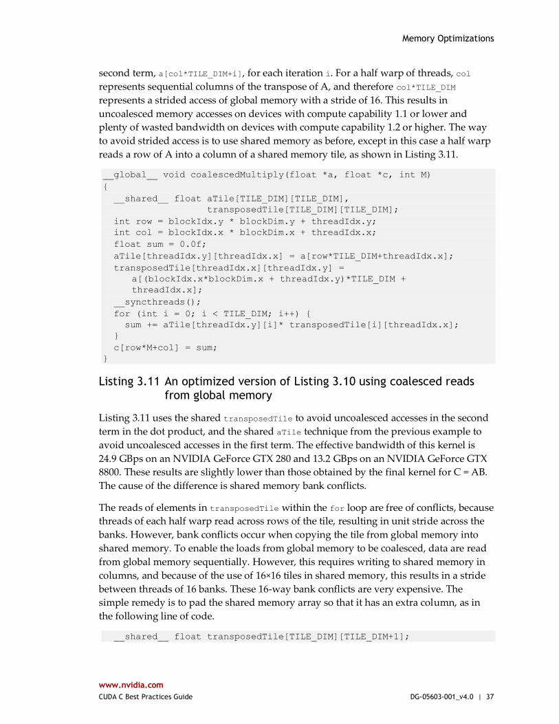
Memory Optimizations
www.nvidia.com
CUDA C Best Practices Guide DG-05603-001_v4.0 | 37
second term, a[col*TILE_DIM+i], for each iteration i. For a half warp of threads, col
represents sequential columns of the transpose of A, and therefore col*TILE_DIM
represents a strided access of global memory with a stride of 16. This results in
uncoalesced memory accesses on devices with compute capability 1.1 or lower and
plenty of wasted bandwidth on devices with compute capability 1.2 or higher. The way
to avoid strided access is to use shared memory as before, except in this case a half warp
reads a row of A into a column of a shared memory tile, as shown in Listing 3.11.
__global__ void coalescedMultiply(float *a, float *c, int M)
{
__shared__ float aTile[TILE_DIM][TILE_DIM],
transposedTile[TILE_DIM][TILE_DIM];
int row = blockIdx.y * blockDim.y + threadIdx.y;
int col = blockIdx.x * blockDim.x + threadIdx.x;
float sum = 0.0f;
aTile[threadIdx.y][threadIdx.x] = a[row*TILE_DIM+threadIdx.x];
transposedTile[threadIdx.x][threadIdx.y] =
a[(blockIdx.x*blockDim.x + threadIdx.y)*TILE_DIM +
threadIdx.x];
__syncthreads();
for (int i = 0; i < TILE_DIM; i++) {
sum += aTile[threadIdx.y][i]* transposedTile[i][threadIdx.x];
}
c[row*M+col] = sum;
}
Listing 3.11 An optimized version of Listing 3.10 using coalesced reads from global memory
Listing 3.11 uses the shared transposedTile to avoid uncoalesced accesses in the second
term in the dot product, and the shared aTile technique from the previous example to
avoid uncoalesced accesses in the first term. The effective bandwidth of this kernel is
24.9 GBps on an NVIDIA GeForce GTX 280 and 13.2 GBps on an NVIDIA GeForce GTX
8800. These results are slightly lower than those obtained by the final kernel for C = AB.
The cause of the difference is shared memory bank conflicts.
The reads of elements in transposedTile within the for loop are free of conflicts, because
threads of each half warp read across rows of the tile, resulting in unit stride across the
banks. However, bank conflicts occur when copying the tile from global memory into
shared memory. To enable the loads from global memory to be coalesced, data are read
from global memory sequentially. However, this requires writing to shared memory in
columns, and because of the use of 16×16 tiles in shared memory, this results in a stride
between threads of 16 banks. These 16-way bank conflicts are very expensive. The
simple remedy is to pad the shared memory array so that it has an extra column, as in
the following line of code.
__shared__ float transposedTile[TILE_DIM][TILE_DIM+1];
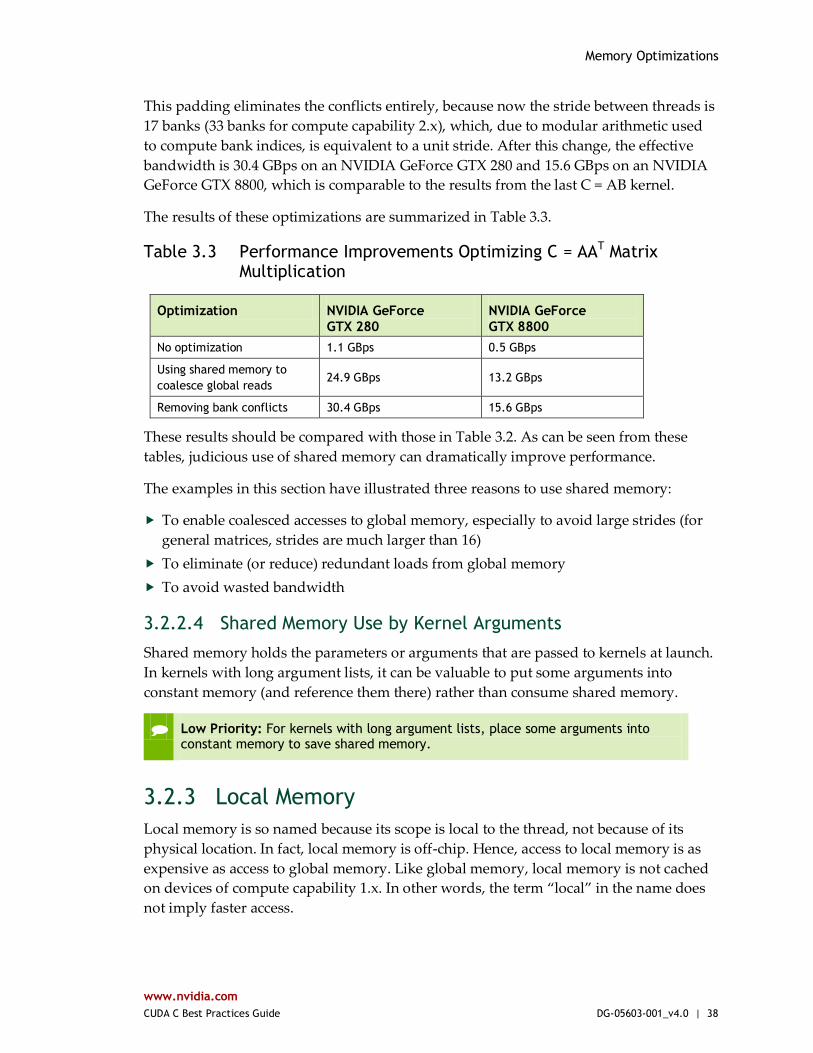
Memory Optimizations
www.nvidia.com
CUDA C Best Practices Guide DG-05603-001_v4.0 | 38
This padding eliminates the conflicts entirely, because now the stride between threads is
17 banks (33 banks for compute capability 2.x), which, due to modular arithmetic used
to compute bank indices, is equivalent to a unit stride. After this change, the effective
bandwidth is 30.4 GBps on an NVIDIA GeForce GTX 280 and 15.6 GBps on an NVIDIA
GeForce GTX 8800, which is comparable to the results from the last C = AB kernel.
The results of these optimizations are summarized in Table 3.3.
Table 3.3 Performance Improvements Optimizing C = AAT Matrix Multiplication
Optimization NVIDIA GeForce
GTX 280
NVIDIA GeForce
GTX 8800
No optimization 1.1 GBps 0.5 GBps
Using shared memory to
coalesce global reads 24.9 GBps 13.2 GBps
Removing bank conflicts 30.4 GBps 15.6 GBps
These results should be compared with those in Table 3.2. As can be seen from these
tables, judicious use of shared memory can dramatically improve performance.
The examples in this section have illustrated three reasons to use shared memory:
To enable coalesced accesses to global memory, especially to avoid large strides (for
general matrices, strides are much larger than 16)
To eliminate (or reduce) redundant loads from global memory
To avoid wasted bandwidth
3.2.2.4 Shared Memory Use by Kernel Arguments
Shared memory holds the parameters or arguments that are passed to kernels at launch.
In kernels with long argument lists, it can be valuable to put some arguments into
constant memory (and reference them there) rather than consume shared memory.
Low Priority: For kernels with long argument lists, place some arguments into constant memory to save shared memory.
3.2.3 Local Memory
Local memory is so named because its scope is local to the thread, not because of its
physical location. In fact, local memory is off-chip. Hence, access to local memory is as
expensive as access to global memory. Like global memory, local memory is not cached
on devices of compute capability 1.x. In other words, the term “local” in the name does
not imply faster access.
Memory Optimizations
www.nvidia.com
CUDA C Best Practices Guide DG-05603-001_v4.0 | 39
Local memory is used only to hold automatic variables. This is done by the nvcc
compiler when it determines that there is insufficient register space to hold the variable.
Automatic variables that are likely to be placed in local memory are large structures or
arrays that would consume too much register space and arrays that the compiler
determines may be indexed dynamically.
Inspection of the PTX assembly code (obtained by compiling with -ptx or -keep
command-line options to nvcc) reveals whether a variable has been placed in local
memory during the first compilation phases. If it has, it will be declared using the .local
mnemonic and accessed using the ld.local and st.local mnemonics. If it has not,
subsequent compilation phases might still decide otherwise, if they find the variable
consumes too much register space for the targeted architecture. There is no way to check
this for a specific variable, but the compiler reports total local memory usage per kernel
(lmem) when run with the --ptxas-options=-v option.
3.2.4 Texture Memory
The read-only texture memory space is cached. Therefore, a texture fetch costs one
device memory read only on a cache miss; otherwise, it just costs one read from the
texture cache. The texture cache is optimized for 2D spatial locality, so threads of the
same warp that read texture addresses that are close together will achieve best
performance. Texture memory is also designed for streaming fetches with a constant
latency; that is, a cache hit reduces DRAM bandwidth demand, but not fetch latency.
In certain addressing situations, reading device memory through texture fetching can be
an advantageous alternative to reading device memory from global or constant memory.
3.2.4.1 Textured Fetch vs. Global Memory Read
Device memory reads through texture fetching present several potential benefits over
reads from global memory:
They are cached, unlike global memory reads in devices of compute capability 1.x.
This results in potentially higher achieved bandwidth if there is 2D locality in the
texture fetches and can be used to avoid uncoalesced loads from global memory.
(Note that the L1 cache in devices of compute capability 2.x has a higher bandwidth
than the texture cache, potentially obviating this benefit in these devices, depending
on access pattern.)
Packed data can be unpacked into separate variables in a single operation.
8-bit and 16-bit integer input data may be optionally converted to 32-bit floating-
point values in the range [0.0, 1.0] or [-1.0, 1.0].
Memory Optimizations
www.nvidia.com
CUDA C Best Practices Guide DG-05603-001_v4.0 | 40
Listings 3.12 and 3.13 illustrate how textures can be used to avoid uncoalesced global
memory accesses in the following variation of the offsetCopy kernel. This copy performs
a shift in data, as demonstrated in the following kernel.
__global__ void shiftCopy(float *odata, float *idata, int shift)
{
int xid = blockIdx.x * blockDim.x + threadIdx.x;
odata[xid] = idata[xid+shift];
}
Listing 3.12 Unoptimized data shifts
This copy kernel applies a shift to the global memory location when reading from idata,
but writes to unshifted global memory locations in odata. The amount of shift is
specified as a function argument to the kernel. Some degradation of performance occurs
when the shift is neither zero nor a multiple of 16 because reading from idata will be
either uncoalesced (compute capability 1.1 or lower) or result in transactions with
wasted bandwidth (compute capability 1.2 or higher). Note that regardless of compute
capability, writing to odata is fully coalesced.
The version of this code that uses textures to perform the shifted read is shown in
Listing 3.13.
__global__ void textureShiftCopy(float *odata, float *idata,
int shift)
{
int xid = blockIdx.x * blockDim.x + threadIdx.x;
odata[xid] = tex1Dfetch(texRef, xid+shift);
}
Listing 3.13 Data shifts optimized by use of texture memory
Here, the texture reference texRef is bound to the idata array in the host code and the
function tex1Dfetch() reads the shifted memory locations of idata via a texture fetch.
The results of both kernels (using global memory and textures for loads) on an NVIDIA
GeForce GTX 280 and an NVIDIA GeForce GTX 8800 are given in Figure 3.12.
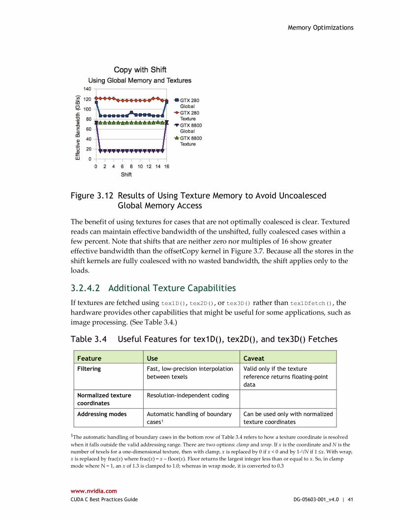
Memory Optimizations
www.nvidia.com
CUDA C Best Practices Guide DG-05603-001_v4.0 | 41
Figure 3.12 Results of Using Texture Memory to Avoid Uncoalesced Global Memory Access
The benefit of using textures for cases that are not optimally coalesced is clear. Textured
reads can maintain effective bandwidth of the unshifted, fully coalesced cases within a
few percent. Note that shifts that are neither zero nor multiples of 16 show greater
effective bandwidth than the offsetCopy kernel in Figure 3.7. Because all the stores in the
shift kernels are fully coalesced with no wasted bandwidth, the shift applies only to the
loads.
3.2.4.2 Additional Texture Capabilities
If textures are fetched using tex1D(), tex2D(), or tex3D() rather than tex1Dfetch(), the
hardware provides other capabilities that might be useful for some applications, such as
image processing. (See Table 3.4.)
Table 3.4 Useful Features for tex1D(), tex2D(), and tex3D() Fetches
Feature Use Caveat
Filtering Fast, low-precision interpolation
between texels
Valid only if the texture
reference returns floating-point
data
Normalized texture
coordinates
Resolution-independent coding
Addressing modes Automatic handling of boundary
cases¹
Can be used only with normalized
texture coordinates
¹The automatic handling of boundary cases in the bottom row of Table 3.4 refers to how a texture coordinate is resolved
when it falls outside the valid addressing range. There are two options: clamp and wrap. If x is the coordinate and N is the
number of texels for a one-dimensional texture, then with clamp, x is replaced by 0 if x < 0 and by 1-1/N if 1 ≤x. With wrap,
x is replaced by frac(x) where frac(x) = x – floor(x). Floor returns the largest integer less than or equal to x. So, in clamp
mode where N = 1, an x of 1.3 is clamped to 1.0; whereas in wrap mode, it is converted to 0.3
Memory Optimizations
www.nvidia.com
CUDA C Best Practices Guide DG-05603-001_v4.0 | 42
Within a kernel call, the texture cache is not kept coherent with respect to global
memory writes, so texture fetches from addresses that have been written via global
stores in the same kernel call return undefined data. That is, a thread can safely read a
memory location via texture if the location has been updated by a previous kernel call or
memory copy, but not if it has been previously updated by the same thread or another
thread within the same kernel call. This is relevant only when fetching from linear or
pitch-linear memory because a kernel cannot write to CUDA arrays.
3.2.4.3 Texture Format Recommendation
For 8-bit texture formats when using OpenGL interoperability, note that interoperating
with GL_RGBA8 textures on devices of compute capability 1.0, 1.1, or 1.3 runs at
reduced performance.
3.2.5 Constant Memory
There is a total of 64 KB constant memory on a device. The constant memory space is
cached. As a result, a read from constant memory costs one memory read from device
memory only on a cache miss; otherwise, it just costs one read from the constant cache.
For all threads of a half warp, reading from the constant cache is as fast as reading from
a register as long as all threads read the same address. Accesses to different addresses by
threads within a half warp are serialized, so cost scales linearly with the number of
different addresses read by all threads within a half warp.
Alternatively, on devices of compute capability 2.x, programs use the LoaD Uniform
(LDU) operation; see Section F.4.4 of the CUDA C Programming Guide for details.
3.2.6 Registers
Generally, accessing a register consumes zero extra clock cycles per instruction, but
delays may occur due to register read-after-write dependencies and register memory
bank conflicts.
The latency of read-after-write dependencies is approximately 24 cycles, but this latency
is completely hidden on multiprocessors that have at least 192 active threads (that is, 6
warps) for devices of compute capability 1.x (8 CUDA cores per multiprocessor * 24
cycles of latency = 192 active threads to cover that latency). For devices of compute
capability 2.0, which have 32 CUDA cores per multiprocessor, as many as 768 threads
might be required to completely hide latency.
The compiler and hardware thread scheduler will schedule instructions as optimally as
possible to avoid register memory bank conflicts. They achieve the best results when the
number of threads per block is a multiple of 64. Other than following this rule, an
Memory Optimizations
www.nvidia.com
CUDA C Best Practices Guide DG-05603-001_v4.0 | 43
application has no direct control over these bank conflicts. In particular, there is no
register-related reason to pack data into float4 or int4 types.
3.2.6.1 Register Pressure
Register pressure occurs when there are not enough registers available for a given task.
Even though each multiprocessor contains thousands of 32-bit registers (see Section F.1
of the CUDA C Programming Guide), these are partitioned among concurrent threads. To
prevent the compiler from allocating too many registers, use the –maxrregcount=N
compiler command-line option (see Section B.1 below) or the launch bounds kernel
definition qualifier (see Section B.17 of the CUDA C Programming Guide) to control the
maximum number of registers to allocated per thread.
3.3 ALLOCATION
Device memory allocation and de-allocation via cudaMalloc() and cudaFree() (or their
Driver API equivalents) are expensive operations, so device memory should be reused
and/or sub-allocated by the application wherever possible to minimize the impact of
allocations on overall performance.
www.nvidia.com
CUDA C Best Practices Guide DG-05603-001_v4.0 | 44
Chapter 4. EXECUTION CONFIGURATION OPTIMIZATIONS
One of the keys to good performance is to keep the multiprocessors on the device as
busy as possible. A device in which work is poorly balanced across the multiprocessors
will deliver suboptimal performance. Hence, it’s important to design your application to
use threads and blocks in a way that maximizes hardware utilization and to limit
practices that impede the free distribution of work. A key concept in this effort is
occupancy, which is explained in the following sections.
Another important concept is the management of system resources allocated for a
particular task. How to manage this resource utilization is discussed in the final sections
of this chapter.
4.1 OCCUPANCY
Thread instructions are executed sequentially in CUDA, and, as a result, executing other
warps when one warp is paused or stalled is the only way to hide latencies and keep the
hardware busy. Some metric related to the number of active warps on a multiprocessor
is therefore important in determining how effectively the hardware is kept busy. This
metric is occupancy.
Occupancy is the ratio of the number of active warps per multiprocessor to the
maximum number of possible active warps. (To determine the latter number, see the
deviceQuery code sample in the GPU Computing SDK or refer to Appendix F in the
CUDA C Programming Guide.) Another way to view occupancy is the percentage of the
hardware’s ability to process warps that is actively in use.
Execution Configuration Optimizations
www.nvidia.com
CUDA C Best Practices Guide DG-05603-001_v4.0 | 45
Higher occupancy does not always equate to higher performance—there is a point
above which additional occupancy does not improve performance. However, low
occupancy always interferes with the ability to hide memory latency, resulting in
performance degradation.
4.2 CALCULATING OCCUPANCY
One of several factors that determine occupancy is register availability. Register storage
enables threads to keep local variables nearby for low-latency access. However, the set
of registers (known as the register file) is a limited commodity that all threads resident on
a multiprocessor must share. Registers are allocated to an entire block all at once. So, if
each thread block uses many registers, the number of thread blocks that can be resident
on a multiprocessor is reduced, thereby lowering the occupancy of the multiprocessor.
The maximum number of registers per thread can be set manually at compilation time
per-file using the –maxrregcount option or per-kernel using the __launch_bounds__
qualifier (see Section 3.2.6.1).
For purposes of calculating occupancy, the number of registers used by each thread is
one of the key factors. For example, devices with compute capability 1.0 and 1.1 have
8,192 32-bit registers per multiprocessor and can have a maximum of 768 simultaneous
threads resident (24 warps x 32 threads per warp). This means that in one of these
devices, for a multiprocessor to have 100% occupancy, each thread can use at most 10
registers. However, this approach of determining how register count affects occupancy
does not take into account the register allocation granularity. For example, on a device of
compute capability 1.0, a kernel with 128-thread blocks using 12 registers per thread
results in an occupancy of 83% with 5 active 128-thread blocks per multiprocessor,
whereas a kernel with 256-thread blocks using the same 12 registers per thread results in
an occupancy of 66% because only two 256-thread blocks can reside on a multiprocessor.
Furthermore, register allocations are rounded up to the nearest 256 registers per block
on devices with compute capability 1.0 and 1.1.
The number of registers available, the maximum number of simultaneous threads
resident on each multiprocessor, and the register allocation granularity vary over
different compute capabilities. Because of these nuances in register allocation and the
fact that a multiprocessor’s shared memory is also partitioned between resident thread
blocks, the exact relationship between register usage and occupancy can be difficult to
determine. The --ptxas-options=-v option of nvcc details the number of registers used
per thread for each kernel. See Section 4.2 of the CUDA C Programming Guide for the
register allocation formulas for devices of various compute capabilities and Section F.1
of the programming guide for the total number of registers available on those devices.
Alternatively, NVIDIA provides an occupancy calculator in the form of an Excel
spreadsheet that enables developers to hone in on the optimal balance and to test
different possible scenarios more easily. This spreadsheet, shown in CUDA GPU
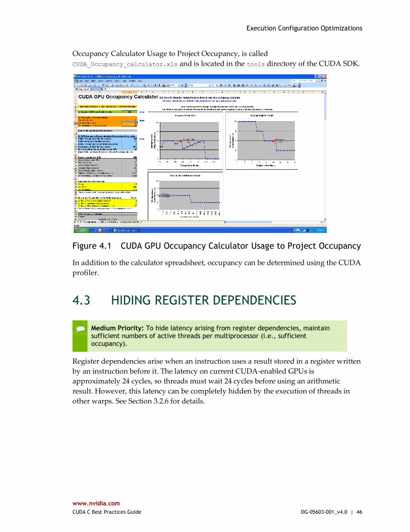
Execution Configuration Optimizations
www.nvidia.com
CUDA C Best Practices Guide DG-05603-001_v4.0 | 46
Occupancy Calculator Usage to Project Occupancy, is called
CUDA_Occupancy_calculator.xls and is located in the tools directory of the CUDA SDK.
Figure 4.1 CUDA GPU Occupancy Calculator Usage to Project Occupancy
In addition to the calculator spreadsheet, occupancy can be determined using the CUDA
profiler.
4.3 HIDING REGISTER DEPENDENCIES
Medium Priority: To hide latency arising from register dependencies, maintain sufficient numbers of active threads per multiprocessor (i.e., sufficient occupancy).
Register dependencies arise when an instruction uses a result stored in a register written
by an instruction before it. The latency on current CUDA-enabled GPUs is
approximately 24 cycles, so threads must wait 24 cycles before using an arithmetic
result. However, this latency can be completely hidden by the execution of threads in
other warps. See Section 3.2.6 for details.
Execution Configuration Optimizations
www.nvidia.com
CUDA C Best Practices Guide DG-05603-001_v4.0 | 47
4.4 THREAD AND BLOCK HEURISTICS
Medium Priority: The number of threads per block should be a multiple of 32 threads, because this provides optimal computing efficiency and facilitates coalescing.
The dimension and size of blocks per grid and the dimension and size of threads per
block are both important factors. The multidimensional aspect of these parameters
allows easier mapping of multidimensional problems to CUDA and does not play a role
in performance. As a result, this section discusses size but not dimension.
Latency hiding and occupancy depend on the number of active warps per
multiprocessor, which is implicitly determined by the execution parameters along with
resource (register and shared memory) constraints. Choosing execution parameters is a
matter of striking a balance between latency hiding (occupancy) and resource
utilization.
Choosing the execution configuration parameters should be done in tandem; however,
there are certain heuristics that apply to each parameter individually. When choosing
the first execution configuration parameter—the number of blocks per grid, or grid size—
the primary concern is keeping the entire GPU busy. The number of blocks in a grid
should be larger than the number of multiprocessors so that all multiprocessors have at
least one block to execute. Furthermore, there should be multiple active blocks per
multiprocessor so that blocks that aren’t waiting for a __syncthreads() can keep the
hardware busy. This recommendation is subject to resource availability; therefore, it
should be determined in the context of the second execution parameter—the number of
threads per block, or block size—as well as shared memory usage. To scale to future
devices, the number of blocks per kernel launch should be in the thousands.
When choosing the block size, it is important to remember that multiple concurrent
blocks can reside on a multiprocessor, so occupancy is not determined by block size
alone. In particular, a larger block size does not imply a higher occupancy. For example,
on a device of compute capability 1.1 or lower, a kernel with a maximum block size of
512 threads results in an occupancy of 66 percent because the maximum number of
threads per multiprocessor on such a device is 768. Hence, only a single block can be
active per multiprocessor. However, a kernel with 256 threads per block on such a
device can result in 100 percent occupancy with three resident active blocks.
As mentioned in Section 4.1, higher occupancy does not always equate to better
performance. For example, improving occupancy from 66 percent to 100 percent
generally does not translate to a similar increase in performance. A lower occupancy
kernel will have more registers available per thread than a higher occupancy kernel,
which may result in less register spilling to local memory. Typically, once an occupancy
Execution Configuration Optimizations
www.nvidia.com
CUDA C Best Practices Guide DG-05603-001_v4.0 | 48
of 50 percent has been reached, additional increases in occupancy do not translate into
improved performance.
There are many such factors involved in selecting block size, and inevitably some
experimentation is required. However, a few rules of thumb should be followed:
Threads per block should be a multiple of warp size to avoid wasting computation on
under-populated warps and to facilitate coalescing.
A minimum of 64 threads per block should be used, but only if there are multiple
concurrent blocks per multiprocessor.
Between 128 and 256 threads per block is a better choice and a good initial range for
experimentation with different block sizes.
Use several (3 to 4) smaller thread blocks rather than one large thread block per
multiprocessor if latency affects performance. This is particularly beneficial to kernels
that frequently call __syncthreads().
Note that when a thread block allocates more registers than are available on a
multiprocessor, the kernel launch fails, as it will when too much shared memory or too
many threads are requested.
4.5 EFFECTS OF SHARED MEMORY
Shared memory can be helpful in several situations, such as helping to coalesce or
eliminate redundant access to global memory. However, it also can act as a constraint on
occupancy. In many cases, the amount of shared memory required by a kernel is related
to the block size that was chosen, but the mapping of threads to shared memory
elements does not need to be one-to-one. For example, it may be desirable to use a 32×32
element shared memory array in a kernel, but because the maximum number of threads
per block is 512, it is not possible to launch a kernel with 32×32 threads per block. In
such cases, kernels with 32×16 or 32×8 threads can be launched with each thread
processing two or four elements, respectively, of the shared memory array. The
approach of using a single thread to process multiple elements of a shared memory
array can be beneficial even if limits such as threads per block are not an issue. This is
because some operations common to each element can be performed by the thread once,
amortizing the cost over the number of shared memory elements processed by the
thread.
A useful technique to determine the sensitivity of performance to occupancy is through
experimentation with the amount of dynamically allocated shared memory, as specified
in the third parameter of the execution configuration. By simply increasing this
parameter (without modifying the kernel), it is possible to effectively reduce the
occupancy of the kernel and measure its effect on performance.
Execution Configuration Optimizations
www.nvidia.com
CUDA C Best Practices Guide DG-05603-001_v4.0 | 49
As mentioned in the previous section, once an occupancy of more than 50 percent has
been reached, it generally does not pay to optimize parameters to obtain higher
occupancy ratios. The previous technique can be used to determine whether such a
plateau has been reached.

www.nvidia.com
CUDA C Best Practices Guide DG-05603-001_v4.0 | 50
Chapter 5. INSTRUCTION OPTIMIZATIONS
Awareness of how instructions are executed often permits low-level optimizations that
can be useful, especially in code that is run frequently (the so-called hot spot in a
program). Best practices suggest that this optimization be performed after all higher-
level optimizations have been completed.
5.1 ARITHMETIC INSTRUCTIONS
Single-precision floats provide the best performance, and their use is highly encouraged.
The throughput of individual arithmetic operations on devices of compute capability 1.x
is detailed in Section F.3 of the CUDA C Programming Guide, and the throughput of
these operations on devices of compute capability 2.x is detailed in Section F.4 of the
programming guide.
5.1.1 Division and Modulo Operations
Low Priority: Use shift operations to avoid expensive division and modulo calculations.
Integer division and modulo operations are particularly costly and should be avoided or
replaced with bitwise operations whenever possible: If n is a power of 2, (i/n) is
equivalent to (i ≫ log2(n)) and (i % n) is equivalent to (i & (n-1)).
The compiler will perform these conversions if n is literal. (For further information, refer
to Chapter 5 of the CUDA C Programming Guide).
Instruction Optimizations
www.nvidia.com
CUDA C Best Practices Guide DG-05603-001_v4.0 | 51
5.1.2 Reciprocal Square Root
The reciprocal square root should always be invoked explicitly as rsqrtf() for single
precision and rsqrt() for double precision. The compiler optimizes 1.0f/sqrtf(x) into
rsqrtf() only when this does not violate IEEE-754 semantics.
5.1.3 Other Arithmetic Instructions
Low Priority: Avoid automatic conversion of doubles to floats.
The compiler must on occasion insert conversion instructions, introducing additional
execution cycles. This is the case for
Functions operating on char or short whose operands generally need to be converted
to an int
Double-precision floating-point constants (defined without any type suffix) used as
input to single-precision floating-point computations
The latter case can be avoided by using single-precision floating-point constants, defined
with an f suffix such as 3.141592653589793f, 1.0f, 0.5f. This suffix has accuracy
implications in addition to its ramifications on performance. The effects on accuracy are
discussed in Chapter 7. Note that this distinction is particularly important to
performance on devices of compute capability 2.x.
For single-precision code, use of the float type and the single-precision math functions
are highly recommended. When compiling for devices without native double-precision
support such as devices of compute capability 1.2 and earlier, each double-precision
floating-point variable is converted to single-precision floating-point format (but retains
its size of 64 bits) and double-precision arithmetic is demoted to single-precision
arithmetic.
It should also be noted that the CUDA math library’s complementary error function,
erfcf(), is particularly fast with full single-precision accuracy.
5.1.4 Math Libraries
Medium Priority: Use the fast math library whenever speed trumps precision.
Two types of runtime math operations are supported. They can be distinguished by
their names: some have names with prepended underscores, whereas others do not (e.g.,
__functionName() versus functionName()). Functions following the __functionName()
naming convention map directly to the hardware level. They are faster but provide
Instruction Optimizations
www.nvidia.com
CUDA C Best Practices Guide DG-05603-001_v4.0 | 52
somewhat lower accuracy (e.g., __sinf(x) and __expf(x)). Functions following
functionName() naming convention are slower but have higher accuracy (e.g., sinf(x)
and expf(x)). The throughput of __sinf(x), __cosf(x), and __expf(x) is much greather
than that of sinf(x), cosf(x), tanf(x). The latter become even more expensive (about
an order of magnitude slower) if the magnitude of the argument x needs to be reduced.
Moreover, in such cases, the argument-reduction code uses local memory, which can
affect performance even more because of the high latency of local memory. More details
are available in the CUDA C Programming Guide.
Note also that whenever sine and cosine of the same argument are computed, the
sincos… family of instructions should be used to optimize performance:
sincosf() for single-precision fast math (see next paragraph)
sincosf() for regular single-precision
sincos() for double precision
The –use_fast_math compiler option of nvcc coerces every functionName() call to the
equivalent __functionName() call. This switch should be used whenever accuracy is a
lesser priority than the performance. This is frequently the case with transcendental
functions. Note this switch is effective only on single-precision floating point.
Medium Priority: Prefer faster, more specialized math functions over slower, more general ones when possible.
For small integer powers (e.g., x2 or x3), explicit multiplication is almost certainly faster
than the use of general exponentiation routines such as pow(). While compiler
optimization improvements continually seek to narrow this gap, explicit multiplication
(or the use of an equivalent purpose-built inline function or macro) can have a
significant advantage. This advantage is increased when several powers of the same
base are needed (e.g., where both x2 and x5 are calculated in close proximity), as this aids
the compiler in its common sub-expression elimination (CSE) optimization.
For exponentiation using base 2 or 10, use the functions exp2() or expf2() and exp10()
or expf10() rather than the functions pow() or powf(). Both pow() and powf() are heavy-
weight functions in terms of register pressure and instruction count due to the
numerous special cases arising in general exponentiation and the difficulty of achieving
good accuracy across the entire ranges of the base and the exponent. The functions
exp2(), exp2f(), exp10(), and exp10f(), on the other hand, are similar to exp() and
expf() in terms of performance, and can be as much as ten times faster than their
pow()/powf() equivalents.
For exponentiation with an exponent of 1/3, use the cbrt() or cbrtf() function rather
than the generic exponentiation functions pow() or powf(), as the former are significantly
faster than the latter. Likewise, for exponentation with an exponent of -1/3, use rcbrt()
or rcbrtf().
Instruction Optimizations
www.nvidia.com
CUDA C Best Practices Guide DG-05603-001_v4.0 | 53
Replace sin(π*<expr>) with sinpi(<expr>) and cos(π*<expr>) with cospi(<expr>). This
is advantageous with regard to both accuracy and performance. As a particular example,
to evaluate the sine function in degrees instead of radians, use sinpi(x/180.0).
Similarly, the single-precision functions sinpif() and cospif() should replace calls to
sinf() and cosf() when the function argument is of the form π*<expr>. (The
performance advantage sinpi() has over sin() is due to simplified argument reduction;
the accuracy advantage is because sinpi() multiplies by π only implicitly, effectively
using an infinitely precise mathematical π rather than a single- or double-precision
approximation thereof.)
Instruction Optimizations
www.nvidia.com
CUDA C Best Practices Guide DG-05603-001_v4.0 | 54
5.2 MEMORY INSTRUCTIONS
High Priority: Minimize the use of global memory. Prefer shared memory access where possible.
Memory instructions include any instruction that reads from or writes to shared, local,
or global memory. When accessing uncached local or global memory, there are 400 to
600 clock cycles of memory latency.
As an example, the assignment operator in the following sample code has a high
throughput, but, crucially, there is a latency of 400 to 600 clock cycles to read data from
global memory:
__shared__ float shared[32];
__device__ float device[32];
shared[threadIdx.x] = device[threadIdx.x];
Much of this global memory latency can be hidden by the thread scheduler if there are
sufficient independent arithmetic instructions that can be issued while waiting for the
global memory access to complete. However, it is best to avoid accessing global memory
whenever possible.
www.nvidia.com
CUDA C Best Practices Guide DG-05603-001_v4.0 | 55
Chapter 6. CONTROL FLOW
6.1 BRANCHING AND DIVERGENCE
High Priority: Avoid different execution paths within the same warp.
Any flow control instruction (if, switch, do, for, while) can significantly affect the
instruction throughput by causing threads of the same warp to diverge; that is, to follow
different execution paths. If this happens, the different execution paths must be
serialized, increasing the total number of instructions executed for this warp. When all
the different execution paths have completed, the threads converge back to the same
execution path.
To obtain best performance in cases where the control flow depends on the thread ID,
the controlling condition should be written so as to minimize the number of divergent
warps.
This is possible because the distribution of the warps across the block is deterministic as
mentioned in Section 4.1 of the CUDA C Programming Guide. A trivial example is when
the controlling condition depends only on (threadIdx / WSIZE) where WSIZE is the warp
size.
In this case, no warp diverges because the controlling condition is perfectly aligned with
the warps.
Control Flow
www.nvidia.com
CUDA C Best Practices Guide DG-05603-001_v4.0 | 56
6.2 BRANCH PREDICATION
Low Priority: Make it easy for the compiler to use branch predication in lieu of loops or control statements.
Sometimes, the compiler may unroll loops or optimize out if or switch statements by
using branch predication instead. In these cases, no warp can ever diverge. The
programmer can also control loop unrolling using
#pragma unroll
For more information on this pragma, refer to the CUDA C Programming Guide.
When using branch predication, none of the instructions whose execution depends on
the controlling condition is skipped. Instead, each such instruction is associated with a
per-thread condition code or predicate that is set to true or false according to the
controlling condition. Although each of these instructions is scheduled for execution,
only the instructions with a true predicate are actually executed. Instructions with a false
predicate do not write results, and they also do not evaluate addresses or read operands.
The compiler replaces a branch instruction with predicated instructions only if the
number of instructions controlled by the branch condition is less than or equal to a
certain threshold: If the compiler determines that the condition is likely to produce
many divergent warps, this threshold is 7; otherwise it is 4.
6.3 LOOP COUNTERS SIGNED VS. UNSIGNED
Medium Priority: Use signed integers rather than unsigned integers as loop counters.
In the C language standard, unsigned integer overflow semantics are well defined,
whereas signed integer overflow causes undefined results. Therefore, the compiler can
optimize more aggressively with signed arithmetic than it can with unsigned arithmetic.
This is of particular note with loop counters: since it is common for loop counters to
have values that are always positive, it may be tempting to declare the counters as
unsigned. For slightly better performance, however, they should instead be declared as
signed.
For example, consider the following code:
for (i = 0; i < n; i++) {
out[i] = in[offset + stride*i];
}
Control Flow
www.nvidia.com
CUDA C Best Practices Guide DG-05603-001_v4.0 | 57
Here, the sub-expression stride*i could overflow a 32-bit integer, so if i is declared as
unsigned, the overflow semantics prevent the compiler from using some optimizations
that might otherwise have applied, such as strength reduction. If instead i is declared as
signed, where the overflow semantics are undefined, the compiler has more leeway to
use these optimizations.
www.nvidia.com
CUDA C Best Practices Guide DG-05603-001_v4.0 | 58
Chapter 7. GETTING THE RIGHT ANSWER
Obtaining the right answer is clearly the principal goal of all computation. On parallel
systems, it is possible to run into difficulties not typically found in traditional serial-
oriented programming. These include threading issues, unexpected values due to the
way floating-point values are computed, and challenges arising from differences in the
way CPU and GPU processors operate. This chapter examines issues that can affect the
correctness of returned data and points to appropriate solutions.
7.1 DEBUGGING
The CUDA debugger, CUDA-GDB, is a valuable debugging tool. It is a port of the GNU
Debugger version 6.6 and runs on 32-bit and 64-bit Linux. See the CUDA-GDB User
Manual for more details.
For Microsoft Windows Vista and 7, the NVIDIA Parallel Nsight debugging and
profiling tool is available as a free plugin for Microsoft Visual Studio. See
http://developer.nvidia.com/object/nsight.html for more details.
7.2 NUMERICAL ACCURACY AND PRECISION
Incorrect or unexpected results arise principally from issues of floating-point accuracy
due to the way floating-point values are computed and stored. The following sections
explain the principal items of interest. Other peculiarities of floating-point arithmetic are
presented in Section F.2 of the CUDA C Programming Guide.
Getting the Right Answer
www.nvidia.com
CUDA C Best Practices Guide DG-05603-001_v4.0 | 59
7.2.1 Single vs. Double Precision
Devices of compute capability 1.3 and higher provide native support for double-
precision floating-point values (that is, values 64 bits wide). Results obtained using
double-precision arithmetic will frequently differ from the same operation performed
via single-precision arithmetic due to the greater precision of the former and due to
rounding issues. Therefore, it is important to be sure to compare like with like and to
express the results within a certain tolerance rather than expecting them to be exact.
Whenever doubles are used, use at least the –arch=sm_13 switch on the nvcc command
line; see Sections 3.1.3 and 3.1.4 of the CUDA C Programming Guide for more details.
7.2.2 Floating-Point Math Is Not Associative
Each floating-point arithmetic operation involves a certain amount of rounding.
Consequently, the order in which arithmetic operations are performed is important. If A,
B, and C are floating-point values, (A+B)+C is not guaranteed to equal A+(B+C) as it is in
symbolic math. When you parallelize computations, you potentially change the order of
operations and therefore the parallel results might not match sequential results. This
limitation is not specific to CUDA, but an inherent part of parallel computation on
floating-point values.
7.2.3 Promotions to Doubles and Truncations to Floats
When comparing the results of computations of float variables between the host and
device, make sure that promotions to double precision on the host do not account for
different numerical results. For example, if the code segment
float a;
…
a = a*1.02;
were performed on a device of compute capability 1.2 or less, or on a device with
compute capability 1.3 but compiled without enabling double precision (as mentioned
above), then the multiplication would be performed in single precision. However, if the
code were performed on the host, the literal 1.02 would be interpreted as a double-
precision quantity and a would be promoted to a double, the multiplication would be
performed in double precision, and the result would be truncated to a float—thereby
yielding a slightly different result. If, however, the literal 1.02 were replaced with 1.02f,
the result would be the same in all cases because no promotion to doubles would occur.
To ensure that computations use single-precision arithmetic, always use float literals.
In addition to accuracy, the conversion between doubles and floats (and vice versa) has
a detrimental effect on performance, as discussed in Chapter 5.
Getting the Right Answer
www.nvidia.com
CUDA C Best Practices Guide DG-05603-001_v4.0 | 60
7.2.4 IEEE 754 Compliance
All CUDA compute devices follow the IEEE 754 standard for binary floating-point
representation, with some small exceptions. These exceptions, which are detailed in
Section F.2 of the CUDA C Programming Guide, can lead to results that differ from IEEE
754 values computed on the host system.
One of the key differences is the fused multiply-add (FMAD) instruction, which
combines multiply-add operations into a single instruction execution and truncates the
intermediate result of the multiplication. Its result will differ at times from results
obtained by doing the two operations separately.
7.2.5 x86 80-bit Computations
x86 processors can use an 80-bit “double extended precision” math when performing
floating-point calculations. The results of these calculations can frequently differ from
pure 64-bit operations performed on the CUDA device. To get a closer match between
values, set the x86 host processor to use regular double or single precision (64 bits and
32 bits, respectively). This is done with the FLDCW assembly instruction or the equivalent
operating system API.
www.nvidia.com
CUDA C Best Practices Guide DG-05603-001_v4.0 | 61
Chapter 8. MULTI-GPU PROGRAMMING
8.1 INTRODUCTION TO MULTI-GPU
Programming a multi-GPU application is no different from programming an application
to utilize multiple cores or sockets because CUDA is completely orthogonal to CPU
thread management or message passing APIs. The only new concept is selecting the
correct GPU, which in most cases is an available GPU (one without an existing context).
In fact, GPU acceleration can be added straightforwardly to existing multi-threaded
CPU code, whether it uses lightweight or heavyweight threads – all one has to do is port
the compute-intensive portions of the code to GPU and add calls to transfer data
between CPU and GPU, leaving the inter-CPU-thread communication code unchanged.
8.2 MULTI-GPU PROGRAMMING
In order to issue work to a GPU, a context (view of a GPU) is established between a CPU
thread (or group of threads) and the GPU. The context contains all of the driver state
that refers to that GPU – the virtual address space, streams, events, allocated blocks of
memory, etc. Only one context can be active on a GPU at any particular instant;
similarly, a CPU thread can execute commands (perform memory allocations, launch
kernels, etc.) in only one context at any particular instant.
A context is established automatically by the CUDA Runtime during the program’s first
call to a function that changes state (such as cudaMalloc(), etc.), so one can force the
creation of a context by calling cudaFree(0). Note that a context is created on GPU 0 by
default, unless another GPU is selected explicitly prior to context creation with a
cudaSetDevice() call. The context is destroyed either by calling cudaDeviceReset()or
when the controlling CPU process exits.
Multi-GPU Programming
www.nvidia.com
CUDA C Best Practices Guide DG-05603-001_v4.0 | 62
In order to issue work to p GPUs concurrently, a program can either use p CPU threads,
each with its own context, or it can use one CPU thread that swaps among several
contexts, or some combination thereof. CPU threads can be lightweight (pthreads,
OpenMP, etc.) or heavyweight (MPI). Note that any CPU multi-threading or message-
passing API or library can be used, as CPU thread management is completely
orthogonal to CUDA. For example, one can add GPU processing to an existing MPI
application by porting the compute-intensive portions of the code without changing the
communication structure.
Even though a GPU can execute calls from one context at a time, it can belong to
multiple contexts. For example, it is possible for several CPU threads to establish
separate contexts with the same GPU (though multiple CPU threads within the same
process accessing the same GPU would normally share the same context by default).
The CUDA driver manages the GPU’s switching among those contexts (switching to the
next waiting context whenever the GPU goes idle) as well as partitioning memory
among the contexts (GPU memory allocated in one context cannot be accessed from
another context since the allocations are in separate virtual address spaces).
8.3 SELECTING A GPU
In many cases, the intent is for each CPU thread to control a different GPU. Achieving
this is straightforward if a program spawns as many lightweight threads as there are
GPUs – one can derive GPU index from thread ID. For example, OpenMP thread ID can
be readily used to select GPUs.
MPI rank can be used to choose a GPU reliably as long as all MPI processes are launched
on a single host node. However, when MPI processes are launched across several
cluster nodes, the assignment of processes to host nodes depends on the MPI
implementation and launch configuration (hostfile), preventing reliable selection of a
unique GPU. To address this issue, one could implement a negotiation protocol among
MPI processes running on the same host (using MPI_Get_processor_name() call), so that
each one claims a unique GPU. A less robust option is for the GPU selection to rely on a
specific allocation MPI processes to nodes (for example, allocating consecutive processes
to the same node).
Starting with CUDA 2.2, Linux drivers provide an alternative and much simpler way to
ensure that each GPU is assigned to at most one context – the administrator can select
exclusive mode via the SMI (System Management Interface) tool that comes with the
driver. In exclusive mode, if the application does not specify a GPU with a
cudaSetDevice() call, the context is no longer created on GPU 0, but on a GPU without
an active context. If there are no available GPUs, or if cudaSetDevice() specifies a GPU
already having an active context, the first CUDA call that attempts to change the device
state will fail and return an error.
Multi-GPU Programming
www.nvidia.com
CUDA C Best Practices Guide DG-05603-001_v4.0 | 63
8.4 INTER-GPU COMMUNICATION
All inter-GPU communication takes place via host nodes. GPU and the controlling CPU
thread communicate via memcopies, while CPU threads exchange data using the same
methods as applications not accelerated with GPUs. Thus, best performance is achieved
when one follows best practices for the CPU-GPU communication as well as CPU-CPU
communication. Note that the two are independent and orthogonal.
Communication between CPU and GPU is most efficient when using pinned memory on
the CPU. Pinned memory enables asynchronous memory copies (allowing for overlap
with both CPU and GPU execution), as well as improves PCIe throughput on FSB
systems. Please refer to the CUDA C Programming Guide for more details and examples
of pinned memory usage.
Lightweight CPU threads exchange data most efficiently via shared memory. Note that
in order for a pinned memory region to be viewed as pinned by CPU threads other than
the one that allocated it, one must call cudaHostAlloc() with the cudaHostAllocPortable
flag. A common communication pattern will be for one CPU thread to copy data from
its GPU to a shared host memory region, after which another CPU thread will copy the
data to its GPU. Users of NUMA systems will have to follow the same best practices as
for communication between non-GPU accelerated CPU threads.
Communication between heavy-weight processes takes place via message passing, for
example MPI. Once data has been copied from GPU to CPU it is transferred to another
process by calling one of the MPI functions. For example, one possible pattern when
exchanging data between two GPUs is for a CPU thread to call a device-to-host
cudaMemcpy(), then MPI_Sendrecv(), then a host-to-device cudaMemcpy(). Note that
performance of the MPI function is not dependent on the fact that data originated at or is
destined for a GPU. Since MPI provides several variations for most of its
communication functions, the choice of a function should be dictated by the best
practices guide for the MPI implementation as well as the system and network.
8.5 COMPILING MULTI-GPU APPLICATIONS
Code that includes GPU kernels or CUDA runtime kernel launch syntax must be
compiled with nvcc, the compiler driver. nvcc invokes either gcc (on Linux) or Microsoft
Visual C++ compiler (on Windows) for non-GPU code. One can pass options to the host
C/C++ compiler through nvcc by using –Xcompiler option (for more details please refer
to nvcc documentation included in the CUDA toolkit). For example, one would specify
nvcc –Xcompiler /openmp in order to pass the -fopenmp option to the host gcc compiler
(the same option for MSVC compiler is /openmp).
Multi-GPU Programming
www.nvidia.com
CUDA C Best Practices Guide DG-05603-001_v4.0 | 64
MPI applications are typically compiled using mpicc, the MPI compiler driver. While it
is possible to pass all the necessary flags through nvcc, it is often simpler to compile MPI
code and CUDA kernel code into separate object files. This approach also fits many
larger projects well, since they separate the communication and computation source
code already.
8.6 INFINIBAND
NVIDIA GPUDirect™ technology allows the sharing of CUDA pinned host memory
with other devices. This allows accelerated transfers of GPU data to other devices, such
as supported Infiniband network adapters. If GPUDirect support is not available for
your network device, network transfer throughput can be reduced. A possible
workaround is to disable RDMA. For the OpenMPI implementation, this can be
achieved by passing the flag –mca btl_openib_flags 1 to mpirun.
www.nvidia.com
CUDA C Best Practices Guide DG-05603-001_v4.0 | 65
Appendix A. RECOMMENDATIONS AND BEST PRACTICES
This appendix contains a list of all the recommendations for optimization and the list of
best practices that are explained in this document.
A.1 Overall Performance Optimization Strategies
Performance optimization revolves around three basic strategies:
Maximizing parallel execution
Optimizing memory usage to achieve maximum memory bandwidth
Optimizing instruction usage to achieve maximum instruction throughput
Maximizing parallel execution starts with structuring the algorithm in a way that
exposes as much data parallelism as possible. Once the parallelism of the algorithm has
been exposed, it needs to be mapped to the hardware as efficiently as possible. This is
done by carefully choosing the execution configuration of each kernel launch. The
application should also maximize parallel execution at a higher level by explicitly
exposing concurrent execution on the device through streams, as well as maximizing
concurrent execution between the host and the device.
Optimizing memory usage starts with minimizing data transfers between the host and
the device because those transfers have much lower bandwidth than internal device data
transfers. Kernel access to global memory also should be minimized by maximizing the
use of shared memory on the device. Sometimes, the best optimization might even be to
avoid any data transfer in the first place by simply recomputing the data whenever it is
needed.
Multi-GPU Programming
www.nvidia.com
CUDA C Best Practices Guide DG-05603-001_v4.0 | 66
The effective bandwidth can vary by an order of magnitude depending on the access
pattern for each type of memory. The next step in optimizing memory usage is therefore
to organize memory accesses according to the optimal memory access patterns. This
optimization is especially important for global memory accesses, because latency of
access costs hundreds of clock cycles. Shared memory accesses, in counterpoint, are
usually worth optimizing only when there exists a high degree of bank conflicts.
As for optimizing instruction usage, the use of arithmetic instructions that have low
throughput should be avoided. This suggests trading precision for speed when it does
not affect the end result, such as using intrinsics instead of regular functions or single
precision instead of double precision. Finally, particular attention must be paid to
control flow instructions due to the SIMT (single instruction multiple thread) nature of
the device.
A.2 High-Priority Recommendations
To get the maximum benefit from CUDA, focus first on finding ways to parallelize
sequential code. (Section 0)
Use the effective bandwidth of your computation as a metric when measuring
performance and optimization benefits. (Section 2.2)
Minimize data transfer between the host and the device, even if it means running
some kernels on the device that do not show performance gains when compared with
running them on the host CPU. (Section 3.1)
Ensure global memory accesses are coalesced whenever possible. (Section 3.2.1)
Minimize the use of global memory. Prefer shared memory access where possible.
(Section 5.2)
Avoid different execution paths within the same warp. (Section 6.1)
A.3 Medium-Priority Recommendations
Accesses to shared memory should be designed to avoid serializing requests due to
bank conflicts. (Section 3.2.2.1)
Use shared memory to avoid redundant transfers from global memory. (Section
3.2.2.2)
To hide latency arising from register dependencies, maintain sufficient numbers of
active threads per multiprocessor (i.e., sufficient occupancy). (Sections 3.2.6 and 4.3)
The number of threads per block should be a multiple of 32 threads, because this
provides optimal computing efficiency and facilitates coalescing. (Section 4.4)
Use the fast math library whenever speed trumps precision. (Section 5.1.4)
Multi-GPU Programming
www.nvidia.com
CUDA C Best Practices Guide DG-05603-001_v4.0 | 67
Prefer faster, more specialized math functions over slower, more general ones when
possible. (Section 5.1.4)
Use signed integers rather than unsigned integers as loop counters. (Section 6.3)
A.4 Low-Priority Recommendations
On version 2.2 of the CUDA Toolkit (and later), use zero-copy operations on
integrated GPUs. (Section 3.1.3)
For kernels with long argument lists, place some arguments into constant memory to
save shared memory. (Section 3.2.2.4)
Use shift operations to avoid expensive division and modulo calculations. (Section
5.1.1)
Avoid automatic conversion of doubles to floats. (Section 5.1.3)
Make it easy for the compiler to use branch predication in lieu of loops or control
statements. (Section 6.2)
www.nvidia.com
CUDA C Best Practices Guide DG-05603-001_v4.0 | 68
Appendix B. NVCC COMPILER SWITCHES
B.1 NVCC
The NVIDIA nvcc compiler driver converts .cu files into C for the host system and
CUDA assembly or binary instructions for the device. It supports a spate of switches, of
which the following are especially useful for optimization and related best practices:
-arch=sm_13 or higher is required for double precision. See Section 7.2.1.
–maxrregcount=N specifies the maximum number of registers kernels can use at a per-
file level. See Section 3.2.6.1. (See also the __launch_bounds__ qualifier discussed in
Section B.17 of the CUDA C Programming Guide to control the number of registers
used on a per-kernel basis.)
--ptxas-options=-v or -Xptxas=-v lists per-kernel register, shared, and constant
memory usage.
–use_fast_math compiler option of nvcc coerces every functionName() call to the
equivalent __functionName() call. This makes the code run faster at the cost of slightly
diminished precision and accuracy. See Section 5.1.4.
www.nvidia.com
CUDA C Best Practices Guide DG-05603-001_v4.0 | 69
Appendix C. REVISION HISTORY
C.1 Version 3.0
Added compute capability 2.0.
Devices of compute capability 2.0 have an L1 cache of configurable size for global and local memory (see Section F.4.1 of the CUDA C Programming Guide). Note that the L1 cache has higher bandwidth than the texture cache and therefore obviates some of the benefits of texture fetch seen in devices of compute capability 1.x. See Section 3.2.4.1.
Removed references to device emulation mode, which is deprecated in CUDA Toolkit 3.0 and will be removed in CUDA Toolkit 3.1.
The CUFFT and CUBLAS libraries can now interoperate with applications that use the Driver API.
Added a recommendation for the use of exp2() or exp10() in preference to pow() to Section
5.1.4.
The __launch_bounds__ kernel definition qualifier can now be used to control register
usage on a per-kernel basis (in contrast to the -maxrregcount command-line option of
nvcc, which controls this on a per-file basis). See Section 3.2.6.1 of this guide and
Section B.17 of the CUDA C Programming Guide.
Note importance of distinguishing single-precision floating-point constants and
arithmetic from double-precision constants and arithmetic for performance on
devices of compute capability 2.0 in Section 5.1.3.
Devices of compute capability 2.0 can multicast shared memory accesses in addition
to the broadcast mechanism in devices of compute capability 1.x.
Added Chapter 8 on multi-GPU programming.
Multi-GPU Programming
www.nvidia.com
CUDA C Best Practices Guide DG-05603-001_v4.0 | 70
C.2 Version 3.1
Added Section 3.3 on memory allocation.
Added fourth bullet to rules of thumb for block size selection in Section 4.4.
Added Section 6.3 on signed versus unsigned loop counters.
C.3 Version 3.2
CUdeviceptr is now a 64-bit value in 64-bit applications, so it is no longer necessary to
cast CUdeviceptr values with (void*)(size_t) when passing them as arguments to
kernels using the CUDA Driver API; this casting is now effectively a no-op. As such,
the type casts have been removed from the example code in Section 1.3.4.
Corrected discussion in Section 3.2.6 of the necessary numbers of active threads per
multiprocessor to hide latency on devices of compute capability 2.0.
C.4 Version 4.0
Added recommendation for the use of explicit multiplication in place of pow() for
small integer powers in Section 5.1.4.
Added recommendations for the use (when applicable) of sinpi(), cospi(), cbrt(),
and rcbrt() in Section 5.1.4.
Modified API recommendation in Section 1.3: most applications should now prefer
the CUDA Runtime API over the CUDA Driver API.
Revised Chapter 8 to better reflect the multi-GPU features of CUDA Toolkit 4.0.
Minor clarifications.
www.nvidia.com
Notice
ALL NVIDIA DESIGN SPECIFICATIONS, REFERENCE BOARDS, FILES, DRAWINGS, DIAGNOSTICS, LISTS, AND OTHER DOCUMENTS (TOGETHER AND SEPARATELY, “MATERIALS”) ARE BEING PROVIDED “AS IS.” NVIDIA MAKES NO
WARRANTIES, EXPRESSED, IMPLIED, STATUTORY, OR OTHERWISE WITH RESPECT TO THE MATERIALS, AND EXPRESSLY DISCLAIMS ALL IMPLIED WARRANTIES OF NONINFRINGEMENT, MERCHANTABILITY, AND FITNESS FOR
A PARTICULAR PURPOSE.
Information furnished is believed to be accurate and reliable. However, NVIDIA Corporation assumes no
responsibility for the consequences of use of such information or for any infringement of patents or other
rights of third parties that may result from its use. No license is granted by implication of otherwise under
any patent rights of NVIDIA Corporation. Specifications mentioned in this publication are subject to change without notice. This publication supersedes and replaces all other information previously supplied. NVIDIA
Corporation products are not authorized as critical components in life support devices or systems without
express written approval of NVIDIA Corporation.
OpenCL
OpenCL is a trademark of Apple Inc. used under license to the Khronos Group Inc.
Trademarks
NVIDIA and the NVIDIA logo are trademarks or registered trademarks of NVIDIA Corporation in the U.S. and
other countries. Other company and product names may be trademarks of the respective companies with which they are associated.
Copyright
© 2011 NVIDIA Corporation. All rights reserved.


![Tuning CUDA Applications for Kepler - Rice University · Tuning CUDA Applications for Kepler DA-06288-001_v7.0 ... and the CUDA C Best Practices Guide [4] ... Tuning CUDA Applications](https://img.pdfslide.us/doc/110x75/5b04868d7f8b9a3c378dc529/tuning-cuda-applications-for-kepler-rice-university-cuda-applications-for-kepler.jpg)