Embed Size (px)
Citation preview

Alma Mater Studiorum · Universita di Bologna
SCUOLA DI SCIENZE
Corso di Laurea Magistrale in Matematica
CUBE COMPLEXES AND
VIRTUAL FIBERING
OF 3-MANIFOLDS
Tesi di Laurea Magistrale in Topologia
Relatore:Chiar.mo Prof.Stefano Francaviglia
Presentata da:Lorenzo Ruffoni
I SessioneAnno Accademico 2012/13

To Nicole

Preface
This thesis is about how geometry, group theory and topology interact
on low-dimensional manifolds, with a special emphasis on the role of non-
positive curvature. The situation is well-understood for surfaces; for instance,
any closed orientable surface is homeomorphic to a sphere, a torus or a surface
with more holes. Moreover the fundamental group is a complete invariant
for surfaces, which means that two surfaces are homeomorphic if and only if
they have isomorphic fundamental groups. As far as geometry is concerned,
each of these surfaces carries a natural Riemannian structure with constant
curvature k, where k ∈ {1, 0,−1} and its precise value depends only on
the topology of the surface (or, equivalently, on its fundamental group); the
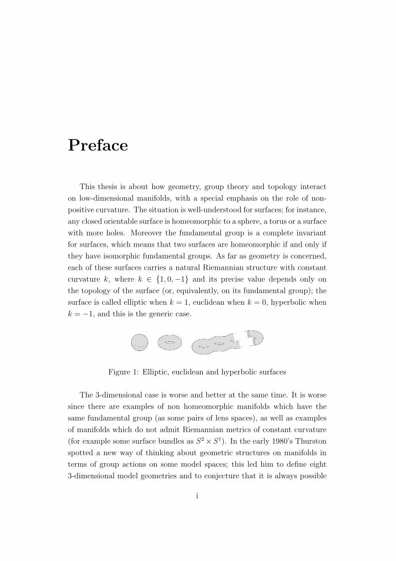
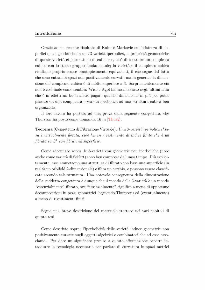
surface is called elliptic when k = 1, euclidean when k = 0, hyperbolic when
k = −1, and this is the generic case.
Figure 1: Elliptic, euclidean and hyperbolic surfaces
The 3-dimensional case is worse and better at the same time. It is worse
since there are examples of non homeomorphic manifolds which have the
same fundamental group (as some pairs of lens spaces), as well as examples
of manifolds which do not admit Riemannian metrics of constant curvature
(for example some surface bundles as S2×S1). In the early 1980’s Thurston
spotted a new way of thinking about geometric structures on manifolds in
terms of group actions on some model spaces; this led him to define eight
3-dimensional model geometries and to conjecture that it is always possible
i
ii Preface
to cut a 3-manifold in pieces which admit one of these geometries. This is
roughly the statement of his celebrated Geometrization Conjecture. Notice
that this is quite worse than the case of surfaces, first of all because we have
to cut, and then because we have to tolerate five rather weird geometries.
One of the main achievements in this approach is due to Perelman, who
in 2003 proved this conjecture. A consequence of his work is that the generic
case is again that of hyperbolic geometry (the manifolds admitting the other
seven geometries have been explicitly classified long before by Seifert). But
this is even better than it looks, since in dimension 3 we have the deep Rigi-
dity Theorem of Mostow, which roughly states that hyperbolic 3-manifolds
are determined up to isometry by their fundamental group. This is quite re-
markable because it means that geometric properties are actually topological
invariants of the underlying manifold.
Hyperbolic 3-manifolds are among the most traditional spaces which dis-
play the typical features of what deserves the name of “non-positively” curved
geometry and it is interesting that the algebraic and combinatorial objects
one associates to them display such properties too, when these are interpreted
in a suitable way. For instance, Gromov introduced the notion of hyperbolic
group motivated by the example of the fundamental groups of hyperbolic
manifolds. These are groups which come equipped with a representation as
isometry groups of a certain associated non-positively curved space.
Many of the properties of these groups can be encoded in combinatorial
structures constructed from some suitable collection of subgroups. These
are the so called cube complexes, which are like simplicial complexes, but
built from cubes instead of simplices, and are the main focus of this the-
sis, together with their application in 3-dimensional topology. As far as the
geometry of codimension 1 subspaces (hyperplanes) is concerned, they have
a much richer structure than simplicial complexes, essentially because you
have two canonical ways of splitting a square into two equal parts, but no
canonical way of splitting a triangle. This simple observation is the basis of
the whole theory of cube complexes.
By a recent result of Kahn and Markovic on the existence of almost
geodesic surfaces in a hyperbolic 3-manifold, the geometric properties of
these manifolds allow us to cubulate them, i.e. to construct a cube com-

Preface iii
plex with the same fundamental group; the manifold and the cube complex
actually turn out to be homotopy equivalent, as an application of their being
non-positively curved, but in general the dimension of the cube complex is
much greater than 3. Remarkably, this is smarter than it sounds: Wise and
Agol have shown in the last few years that it is indeed a great deal to pay
some extra dimensions to get from a wild hyperbolic 3-manifold to a well
organized cubical structure.
Their work has led to a proof of the following conjecture, which Thurston
posed as question 16 in [Thu82]:
Theorem (Virtually Fibered Conjecture). A closed hyperbolic 3-manifold is
virtually fibered, i.e. it has a finite index covering space which is a bundle
over S1 with fiber a surface.
As hinted above, non hyperbolic geometric 3-manifolds (also known as
Seifert manifolds) have been very well understood since a long time. To
be more specific, they admit the structure of a fiber bundle with base a
surface (actually a 2-dimensional orbifold) and fiber a circle, and can be
classified according to this structure. Therefore a striking consequence of the
proof of the above conjecture is that the world of 3-dimensional manifolds
is “essentially” a fibered world, where “essentially” means up to a suitable
decomposition in geometric pieces (following Thurston) and (possibly) up to
finite covers.
Here is an outline of the material covered in the chapters in this thesis.
As described above, the hyperbolicity of manifolds induces non-positively
curved phenomena in the algebraic and combinatorial objects we associate
to them. To give a precise meaning to this sentence we need to introduce
the necessary machinery to talk about curvature in abstract metric spaces,
which we do in Chapter 1. We also introduce the right notion of equivalence
under which these phenomena are preserved, i.e. quasi-isometry.
Groups arise naturally in geometric concrete examples as fundamental
groups of topological spaces or isometry groups of metric spaces. In Chapter

iv Preface
2 we show that indeed any abstract (finitely presented) group can be realized
as a fundamental group and as an isometry grou, of some suitably constructed
spaces. We discuss applications of this point of view to the relationship
between homotopy and cohomology of CW complexes and introduce the
notion of hyperbolic group.
Chapter 3 is about cube complexes and their hyperplanes (= codimen-
sion 1 subspaces). We especially focus on some conditions on the way these
hyperplanes sit and intersect inside the complex, which are known as specia-
lity conditions. The interest in special cube complexes is due to their close
relationship wiht right-angled Artin groups, which are a class of groups with
a quite easy presentation and nice topological and geometric properties.
In order to understand how and why hyperbolic geometry turns out to
be so fundamental in the study of 3-manifolds, in Chapter 4 we describe the
classic decomposition techniques of 3-dimensional topology and the geometric
program initiated by Thurston and closed by Perelman.
The final chapter shows how to apply the geometric (Chapter 1), algebraic
(Chapter 2) and combinatorial (Chapter 3) techniques developed before to
the study of virtual fibrations of closed hyperbolic 3-manifolds, which, by
the reductions of Chapter 4, are the only case which is not fully understood.
We present the work (especially by Wise and Agol) on how to go from a
closed hyperbolic 3-manifold to a special cube complex and then to a virtual
fibration of the manifold.

Introduzione
Questa tesi tratta delle interazioni tra geometria, teoria dei gruppi e
topologia su varieta di dimensione bassa, con attenzione particolare al ruolo
della curvatura non positiva. La situazione e ben nota nel caso delle super-
fici; ad esempio, ogni superficie chiusa orientabile e omeomorfa a una sfera,
un toro o una superficie con piu buchi. Inoltre il gruppo fondamentale e
un invariante completo per le superfici, cioe due superfici sono omeomorfe
se e solo se hanno lo stesso gruppo fondamentale. Per quanto riguarda la
geometria, ciascuna di queste superfici ammette una naturale struttura Rie-
manniana a curvatura costante k, con k ∈ {1, 0,−1}, il cui preciso valore
dipende solo dalla topologia della superficie (o, equivalentemente, dal suo
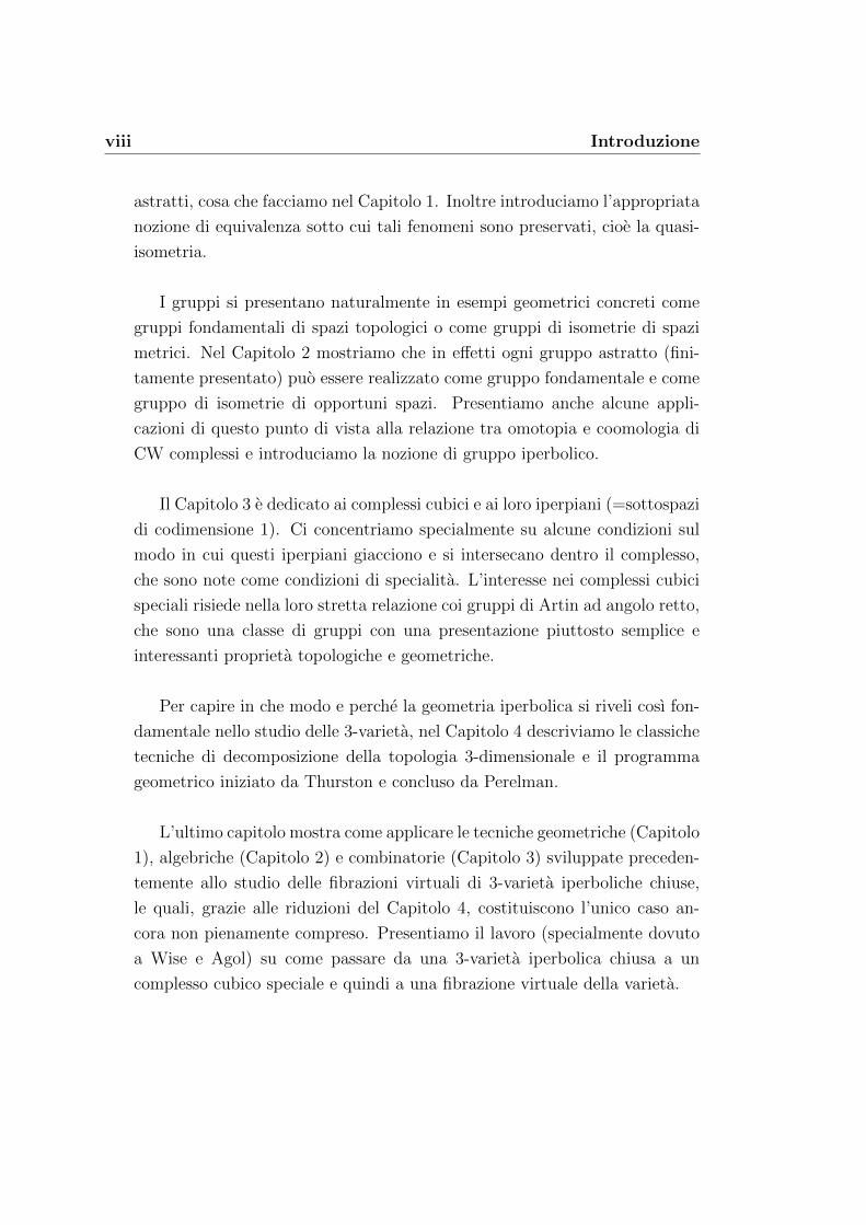
gruppo fondamentale); la superficie si dice ellittica per k = 1, euclidea per
k = 0 e iperbolica per k = −1, e questo e il caso generico.
Figure 2: Superficie ellittica, euclidea e iperbolica
Il caso 3-dimensionale e allo stesso tempo migliore e peggiore. E peg-
giore in quanto ci sono esempi di varieta non omeomorfe che hanno lo stesso
gruppo fondamentale (come certe coppie di spazi lenticolari), cosı come ci
sono esempi di varieta che non ammettono metriche di Riemann a curvatura
costante (ad esempio certi fibrati con fibra una superficie, come S2 × S1).
All’inizio degli anni 1980 Thurston ha individuato un nuovo modo di pen-
sare le strutture geometriche su varieta in termini di azioni di gruppi su certi
v
vi Introduzione
spazi modello; questa impostazione lo ha condotto a definire otto geome-
trie modello 3-dimensionali e a congetturare che sia sempre possibile tagliare
una 3-varieta in pezzi che ammettano una di queste geometrie. Questo e
all’incirca l’enunciato della sua celebre Congettura di Geometrizzazione. Si
noti che questo caso e alquanto peggiore di quello delle superfici, prima di
tutto perche dobbiamo eseguire una decomposizione, e poi perche dobbiamo
tollerare cinque geometrie piuttosto strane.
Uno dei successi principali in questo approccio e dovuto a Perelman, che
nel 2003 ha provato tale congettura. Una conseguenza del suo lavoro e che il
caso generico e ancora quello della geometria iperbolica (le varieta che am-
mettono le altre sette geometrie sono state classificate tempo fa da Seifert).
Cio e anche migliore di quel che sembra, in quanto in dimensione 3 abbiamo
il profondo Teorema di Rigidita di Mostow, che essenzialmente afferma che
le 3-varieta iperboliche sono determinate a meno di isometria dal loro gruppo
fondamentale. Questo e davvero notevole, in quanto implica che le proprieta
geometriche sono in effetti invarianti topologici della varieta soggiacente.
Le 3-varieta iperboliche sono tra gli spazi piu tradizionali che manifestano
le caratteristiche tipiche di cio che merita il nome di geometria “non positi-
vamente curvata” ed e interessante che gli oggetti algebrici e combinatori che
associamo loro manifestano anch’essi tali proprieta. Ad esempio Gromov ha
introdotto la nozione di gruppo iperbolico, motivata dall’esempio del gruppo
fondamentale di una varieta iperbolica. Si tratta di gruppi che ammettono
una rappresentazione come gruppi di isometrie di opportuni spazi non posi-
tivamente curvati.
Molte delle proprieta di questi gruppi possono essere codificate con strut-
ture combinatorie costruite a partire da opportune collezioni di sottogruppi.
Questi sono i cosiddetti complessi cubici, che sono simili ai complessi simpli-
ciali, ma costruiti a partire da cubi anziche da simplessi, e sono il fulcro princi-
pale di questa tesi, assieme alla loro applicazione in topologia 3-dimensionale.
Per quanto riguarda la geometria dei sottospazi di codimensione 1 (iperpiani),
essi godono di una struttura molto piu ricca dei complessi simpliciali, essen-
zialmente perche ci sono due modi canonici di dividere a meta un quadrato,
ma non ci sono modi canonici di dividere a meta un triangolo. Questa sem-
plice osservazione e alla base dell’intera teoria dei complessi cubici.
Introduzione vii
Grazie ad un recente risultato di Kahn e Markovic sull’esistenza di su-
perfici quasi geodetiche in una 3-varieta iperbolica, le proprieta geometriche
di queste varieta ci permettono di cubularle, cioe di costruire un complesso
cubico con lo stesso gruppo fondamentale; la varieta e il complesso cubico
risultano proprio essere omotopicamente equivalenti, il che segue dal fatto
che sono entrambi spazi non positivamente curvati, ma in generale la dimen-
sione del complesso cubico e di molto superiore a 3. Sorprendentemente cio
non e cosı male come sembra: Wise e Agol hanno mostrato negli ultimi anni
che e in effetti un buon affare pagare qualche dimensione in piu per poter
passare da una complicata 3-varieta iperbolica ad una struttura cubica ben
organizzata.
Il loro lavoro ha portato ad una prova della seguente congettura, che
Thurston ha posto come domanda 16 in [Thu82]:
Teorema (Congettura di Fibrazione Virtuale). Una 3-varieta iperbolica chiu-
sa e virtualmente fibrata, cioe ha un rivestimento di indice finito che e un
fibrato su S1 con fibra una superficie.
Come accennato sopra, le 3-varieta con geometrie non iperboliche (note
anche come varieta di Seifert) sono ben comprese da lungo tempo. Piu esplici-
tamente, esse ammettono una struttura di fibrato con base una superficie (in
realta un orbifold 2-dimensionale) e fibra un cerchio, e possono essere classifi-
cate secondo tale struttura. Una notevole conseguenza della dimostrazione
della suddetta congettura e dunque che il mondo delle 3-varieta e un mondo
“essenzialmente” fibrato, ove “essenzialmente” significa a meno di opportune
decomposizioni in pezzi geometrici (seguendo Thurston) ed (eventualmente)
a meno di rivestimenti finiti.
Segue una breve descrizione del materiale trattato nei vari capitoli di
questa tesi.
Come descritto sopra, l’iperbolicita delle varieta induce geometrie non
positivamente curvate sugli oggetti algebrici e combinatori che ad esse asso-
ciamo. Per dare un significato preciso a questa affermazione occorre in-
trodurre la tecnologia necessaria per parlare di curvatura in spazi metrici
viii Introduzione
astratti, cosa che facciamo nel Capitolo 1. Inoltre introduciamo l’appropriata
nozione di equivalenza sotto cui tali fenomeni sono preservati, cioe la quasi-
isometria.
I gruppi si presentano naturalmente in esempi geometrici concreti come
gruppi fondamentali di spazi topologici o come gruppi di isometrie di spazi
metrici. Nel Capitolo 2 mostriamo che in effetti ogni gruppo astratto (fini-
tamente presentato) puo essere realizzato come gruppo fondamentale e come
gruppo di isometrie di opportuni spazi. Presentiamo anche alcune appli-
cazioni di questo punto di vista alla relazione tra omotopia e coomologia di
CW complessi e introduciamo la nozione di gruppo iperbolico.
Il Capitolo 3 e dedicato ai complessi cubici e ai loro iperpiani (=sottospazi
di codimensione 1). Ci concentriamo specialmente su alcune condizioni sul
modo in cui questi iperpiani giacciono e si intersecano dentro il complesso,
che sono note come condizioni di specialita. L’interesse nei complessi cubici
speciali risiede nella loro stretta relazione coi gruppi di Artin ad angolo retto,
che sono una classe di gruppi con una presentazione piuttosto semplice e
interessanti proprieta topologiche e geometriche.
Per capire in che modo e perche la geometria iperbolica si riveli cosı fon-
damentale nello studio delle 3-varieta, nel Capitolo 4 descriviamo le classiche
tecniche di decomposizione della topologia 3-dimensionale e il programma
geometrico iniziato da Thurston e concluso da Perelman.
L’ultimo capitolo mostra come applicare le tecniche geometriche (Capitolo
1), algebriche (Capitolo 2) e combinatorie (Capitolo 3) sviluppate preceden-
temente allo studio delle fibrazioni virtuali di 3-varieta iperboliche chiuse,
le quali, grazie alle riduzioni del Capitolo 4, costituiscono l’unico caso an-
cora non pienamente compreso. Presentiamo il lavoro (specialmente dovuto
a Wise e Agol) su come passare da una 3-varieta iperbolica chiusa a un
complesso cubico speciale e quindi a una fibrazione virtuale della varieta.
Contents
Preface i
Introduzione v
1 Non-Positively Curved Geometries 1
1.1 Preliminaries about Metric Spaces . . . . . . . . . . . . . . . . 1
1.2 CAT(k) Condition . . . . . . . . . . . . . . . . . . . . . . . . 4
1.3 Quasi-isometries . . . . . . . . . . . . . . . . . . . . . . . . . . 6
1.4 δ-Hyperbolicity . . . . . . . . . . . . . . . . . . . . . . . . . . 9
1.4.1 The Boundary at ∞ . . . . . . . . . . . . . . . . . . . 10
1.4.2 The Ends . . . . . . . . . . . . . . . . . . . . . . . . . 11
2 The Geometric and Topological Approach to Group Theory 13
2.1 Groups as Fundamental Groups . . . . . . . . . . . . . . . . . 14
2.1.1 Presentation Complex . . . . . . . . . . . . . . . . . . 14
2.1.2 Eilenberg-MacLane Spaces . . . . . . . . . . . . . . . . 16
2.2 Groups as Isometry Groups . . . . . . . . . . . . . . . . . . . 19
2.2.1 Cayley Graph . . . . . . . . . . . . . . . . . . . . . . . 19
2.2.2 Cayley Complex . . . . . . . . . . . . . . . . . . . . . . 23
2.3 Hyperbolic Groups . . . . . . . . . . . . . . . . . . . . . . . . 25
3 Special Cube Complexes 27
3.1 Hyperplanes and Walls in Cube Complexes . . . . . . . . . . . 27
3.2 Speciality Conditions . . . . . . . . . . . . . . . . . . . . . . . 31
3.2.1 Virtual Equivalence . . . . . . . . . . . . . . . . . . . . 33
3.3 Virtual Embedding in RAAGs . . . . . . . . . . . . . . . . . . 37
ix

x CONTENTS
3.3.1 Right-Angled Artin Groups . . . . . . . . . . . . . . . 37
3.3.2 A-typing of a Square Complex . . . . . . . . . . . . . . 39
3.4 Non-Positively Curved Cube Complexes . . . . . . . . . . . . 42
4 Decompositions of 3-Manifolds 45
4.1 Prime Decomposition . . . . . . . . . . . . . . . . . . . . . . . 46
4.2 Incompressible Surfaces . . . . . . . . . . . . . . . . . . . . . . 49
4.3 JSJ Decomposition . . . . . . . . . . . . . . . . . . . . . . . . 52
4.3.1 Seifert Manifolds . . . . . . . . . . . . . . . . . . . . . 53
4.4 Geometric Decomposition . . . . . . . . . . . . . . . . . . . . 54
4.4.1 Geometric Structures on Manifolds . . . . . . . . . . . 55
4.4.2 Thurston’s Eight Geometries . . . . . . . . . . . . . . . 57
4.4.3 A comparison between JSJ and Geometric Decompo-
sition . . . . . . . . . . . . . . . . . . . . . . . . . . . . 59
4.4.4 Hyperbolic Geometry . . . . . . . . . . . . . . . . . . . 60
4.5 Haken Manifolds . . . . . . . . . . . . . . . . . . . . . . . . . 62
5 Virtual Fibration of Hyperbolic 3-manifolds 67
5.1 Cubulation of Groups and Manifolds . . . . . . . . . . . . . . 69
5.1.1 Codimension-1 Subgroups . . . . . . . . . . . . . . . . 69
5.1.2 Surface Subgroups . . . . . . . . . . . . . . . . . . . . 73
5.1.3 Agol’s Virtual Compact Special Theorem . . . . . . . . 75
5.2 From RAAG to Fibrations . . . . . . . . . . . . . . . . . . . . 78
5.2.1 Residually Finite Rationally Solvable Groups . . . . . . 78
5.2.2 Right-Angled Coxeter Groups . . . . . . . . . . . . . . 82
5.2.3 Thurston’s Norm on Homology . . . . . . . . . . . . . 85
5.2.4 Virtual Fibration of RFRS Manifolds . . . . . . . . . . 87
Bibliography 93
List of Figures
1 Elliptic, euclidean and hyperbolic surfaces . . . . . . . . . . . i
2 . . . . . . . . . . . . . . . . . . . . . . . . . . . . . . . . . . . v
1.1 The CAT(k) condition . . . . . . . . . . . . . . . . . . . . . . 4
1.2 A δ-slim triangle . . . . . . . . . . . . . . . . . . . . . . . . . 9
2.1 The Cayley Graph of F2, the free group on two generators . . 21
2.2 (A portion of) the Cayley Graph of Z with respect to {1} . . . 22
2.3 (A portion of) the Cayley Graph of Z with respect to {2, 3} . 23
3.1 A cube complex . . . . . . . . . . . . . . . . . . . . . . . . . . 28
3.2 Midcubes in I2 and I3 . . . . . . . . . . . . . . . . . . . . . . 28
3.3 A hyperplane in a cube complex . . . . . . . . . . . . . . . . . 29
3.4 A selfintersecting hyperplane . . . . . . . . . . . . . . . . . . . 31
3.5 A 1-sided hyperplane . . . . . . . . . . . . . . . . . . . . . . . 32
3.6 A directly selfosculating hyperplane (left) and an indirectly
selfosculating hyperplane (right) . . . . . . . . . . . . . . . . . 32
3.7 A pair of interosculating hyperplanes . . . . . . . . . . . . . . 33
3.8 Three graphs, giving rise respectively to to F5, F2 × F3 and Z5 38
3.9 The presentation complex for A(•−−•−−•−−•) . . . . . . . . . . 38
4.1 An incompressible surface . . . . . . . . . . . . . . . . . . . . 50
xi

xii LIST OF FIGURES

Chapter 1
Non-Positively Curved
Geometries
The Uniformization Theorem for surfaces shows that hyperbolic geometry
is the most common in dimension 2. In Chapter 4 we will describe the
work of Thurston and Perelman on the geometrization of 3-manifolds, which
reveals that the same is true in dimension 3. This is a nice fact, since non-
positively curved shapes exhibit a lot of interesting features from a geometric
and homotopical point of view.
Some of these properties do not actually rely to the locally euclidean
structure of hyperbolic manifolds, and in this chapter we will describe a
generalization of hyperbolic geometry to abstract metric spaces. This will be
applied to groups and cube complexes in the following chapters.
1.1 Preliminaries about Metric Spaces
In this section we collect the basics definition about metric spaces, stress-
ing the analogy with the case of Riemannian manifolds.
Definition 1.1.1. Let (X, d) be a metric space. A geodesic from x ∈ X to
y ∈ X is a continuous path γ : [0, L] → X from x to y such that for all
s, t ∈ [0, L] we have d(γ(s), γ(t)) = |s− t| .
Example 1.1.2. If (M, g) is a Riemannian manifold, then length minimizing
Riemannian geodesics are geodesics in the above sense, by definition of the
1

2 1. Non-Positively Curved Geometries
Riemannian distance dg associated to the Riemannian metric g. Notice that
not all geodesics on a sphere are geodesics in the above sense (since some are
not length minimizing).
Definition 1.1.3. A metric space (X, d) is said to be
• a geodesic space if every couple of points is joined by a geodesic;
• a uniquely geodesic space if every couple of points is joined by a unique
geodesic; we also say X is R-uniquely geodesic if its balls of radius at
most R are uniquely geodesic;
• a length space if ∀ x, y ∈ X we have that d(x, y) = inf{L(γ)|γ is a
geodesic joining x and y}; if there are no geodesics joining x and y we
agree to say that d(x, y) =∞;
• a proper space if closed balls are compact;
• a cocompact space if it admits a compact subset K whose translates
under the action of Isom(X) cover the whole space.
A geodesic space is a length space, right away from the above definitions.
To see how in general things can go wrong we consider a few examples.
Example 1.1.4. S1 with the distance induced by the euclidean distance
of R2 (i.e. the chord distance) is not a length space (and so it is neither
geodesic). But if we equip it with the Riemannian metric induced by R2 (i.e.
the arc length) and consider the associated path metric then it becomes a
geodesic space.
Example 1.1.5. The punctured plane R2 \ {0} is a length space which is
not geodesic.
The point in the last example is the failure of completeness. We have the
following classical result.
Theorem 1.1.6 (Hopf, Rinow). A connected, complete and locally compact
length space is a geodesic space.

1.1 Preliminaries about Metric Spaces 3
For a detailed proof see [BrH99], Proposition 3.7. This result of course
applies to complete connected Riemannian manifolds when considered as
metric spaces with respect to the path metric (see [BrH99], Corollary I.3.20).
Notice anyway that in general these spaces can fail to be uniquely geodesic,
as the example of spheres shows.
We now introduce a family of metric spaces which come from classic
Riemannian manifolds of constant curvature and will be used as model spaces
to induce a notion of curvature on more general metric spaces.
Definition 1.1.7. For each real number k let Mnk denote the following metric
space:
• if k = 0 then Mnk = En with the euclidean metric;
• if k > 0 then Mnk is obtained from Sn by multiplying the distance
function by k−1/2;
• if k < 0 then Mnk is obtained from Hn by multiplying the distance
function by (−k)−1/2.
We also denote by Dk the diameter of Mnk , i.e. Dk = π
kfor k > 0 and Dk =∞
otherwise.
In the following sections we will introduce the machinery needed to speak
of curvature in an abstract metric space. Two different approaches (and the
relationship between them) are discussed.
Both approaches are based on some kind of consideration about triangles,
so we advance this definition.
Definition 1.1.8. Let (X, d) be a metric space. A geodesic triangle ∆ in
X consists of three vertices p, q, r ∈ X and a choice of three geodesics which
will be denoted [p, q], [q, r] and [r, p] and called the edges of the triangle. The
triangle will also be denoted by ∆([p, q], [q, r], [r, p]) or just ∆(p, q, r) (even if
this may cause some confusion when the space is not uniquely geodesic).

4 1. Non-Positively Curved Geometries
1.2 CAT(k) Condition
The approach we discuss in this section stems from the work of Cartan,
Alexandrov and Toponogov and is based on the comparison with the model
spaces defined in 1.1.7. In the sequel of this section (X, d) will denote a
geodesic metric space.
Definition 1.2.1. Let ∆ = ∆(x1, x2, x3) ⊂ X be a geodesic triangle. A k-
comparison triangle is a geodesic triangle ∆ = ∆(x1, x2, x3) ⊂M2k such that
d(xi, xj) = d(xi, xj), where d denotes the distance in M2k . A point x ∈ [xi, xj]
is called a comparison point for a point x ∈ [xi, xj] if d(xi, x) = d(xi, x).
We of course need the following result, which is Lemma I.2.14 in [BrH99].
Lemma 1.2.2. Let ∆ ⊂ X be a geodesic triangle and k ∈ R. If its perimeter
is less than 2Dk then there exists a k-comparison triangle and it is unique up
to isometry of M2k .
We are now ready to give the main definition of this section:
Definition 1.2.3. Let k ∈ R. A geodesic triangle ∆ ⊂ X is said to satisfy
the CAT(k) condition if its perimeter is less than 2Dk and if for all x, y ∈ ∆
and for all comparison points x, y in a k-comparison triangle ∆ we have that
d(x, y) ≤ d(x, y).
Figure 1.1: The CAT(k) condition
Definition 1.2.4. A space X is called a CAT(k) space if it is geodesic and its
geodesic triangles satisfy the CAT(k) condition. It is said to have curvature
≤ k if it is locally CAT(k).
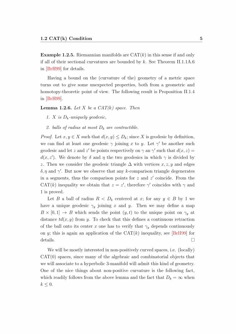
1.2 CAT(k) Condition 5
Example 1.2.5. Riemannian manifolds are CAT(k) in this sense if and only
if all of their sectional curvatures are bounded by k. See Theorem II.1.1A.6
in [BrH99] for details.
Having a bound on the (curvature of the) geometry of a metric space
turns out to give some unexpected properties, both from a geometric and
homotopy-theoretic point of view. The following result is Proposition II.1.4
in [BrH99].
Lemma 1.2.6. Let X be a CAT(k) space. Then
1. X is Dk-uniquely geodesic,
2. balls of radius at most Dk are contractible.
Proof. Let x, y ∈ X such that d(x, y) ≤ Dk; since X is geodesic by definition,
we can find at least one geodesic γ joining x to y. Let γ′ be another such
geodesic and let z and z′ be points respectively on γ an γ′ such that d(x, z) =
d(x, z′). We denote by δ and η the two geodesics in which γ is divided by
z. Then we consider the geodesic triangle ∆ with vertices x, z, y and edges
δ, η and γ′. But now we observe that any k-comparison triangle degenerates
in a segments, thus the comparison points for z and z′ coincide. From the
CAT(k) inequality we obtain that z = z′, therefore γ′ coincides with γ and
1 is proved.
Let B a ball of radius R < Dk centered at x; for any y ∈ B by 1 we
have a unique geodesic γy joining x and y. Then we may define a map
B × [0, 1] → B which sends the point (y, t) to the unique point on γy at
distance td(x, y) from y. To check that this defines a continuous retraction
of the ball onto its center x one has to verify that γy depends continuously
on y; this is again an application of the CAT(k) inequality, see [BrH99] for
details.
We will be mostly interested in non-positively curved spaces, i.e. (locally)
CAT(0) spaces, since many of the algebraic and combinatorial objects that
we will associate to a hyperbolic 3-manifold will admit this kind of geometry.
One of the nice things about non-positive curvature is the following fact,
which readily follows from the above lemma and the fact that Dk =∞ when
k ≤ 0.

6 1. Non-Positively Curved Geometries
Corollary 1.2.7. For any k ≤ 0, a CAT(k) space is contractible.
This allows to extend many classic results about non-positively curved
Riemannian manifolds to this more general context. For example, from a
generalization of the Cartan-Hadamard Theorem one can prove the following
useful result, which is Proposition II.4.14 in [BrH99].
Theorem 1.2.8. Let X and Y be complete connected metric spaces; suppose
that X is locally a length space and that Y is non-positively curved. Let
f : X → Y be a locally isometric embedding. Then
• X is non-positively curved,
• the induced map f∗ : π1(X)→ π1(Y ) is injective.
1.3 Quasi-isometries
In this section we introduce a notion of metric equivalence which is strictly
weaker than isometry, but is the right thing to consider for the application
to group theory we will develop in the next chapter.
Definition 1.3.1. Let (X, dX) and (Y, dY ) be metric spaces and f : X → Y a
(not necessarily continuous) function . Then we give the following definitions:
• if ∃ λ ≥ 1, ε ≥ 0 such that ∀ p, q ∈ X we have
1
λdX(p, q)− ε ≤ dY (f(p), f(q)) ≤ λdX(p, q) + ε
then we say that f is a (λ, ε)-quasi-isometric embedding ;
• if ∃ λ ≥ 1, ε ≥ 0 such that f is a (λ, ε)-quasi-isometric embedding
and ∃ C ≥ 0 such that ∀ y ∈ Y we have that y belongs to the C-
neighbourhood of the image of f , then we say that f is a (λ, ε)-quasi-
isometry.
When we do not care about the constants involved, we just say that f is
a quasi-isometric embedding (respectively, a quasi-isometry) if it is a (λ, ε)-
quasi-isometric embedding (respectively, a (λ, ε)-quasi-isometry) for some
λ ≥ 1, ε ≥ 0.
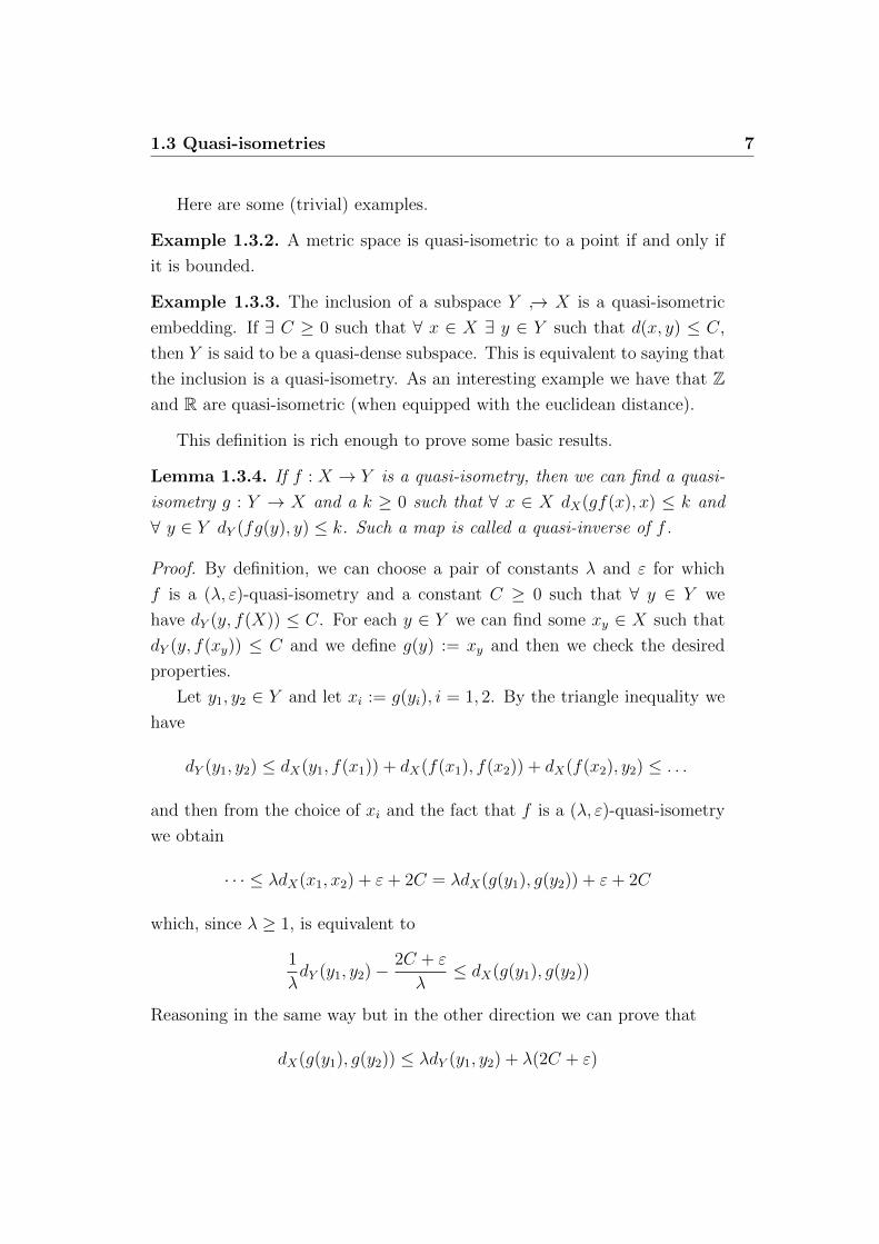
1.3 Quasi-isometries 7
Here are some (trivial) examples.
Example 1.3.2. A metric space is quasi-isometric to a point if and only if
it is bounded.
Example 1.3.3. The inclusion of a subspace Y ↪→ X is a quasi-isometric
embedding. If ∃ C ≥ 0 such that ∀ x ∈ X ∃ y ∈ Y such that d(x, y) ≤ C,
then Y is said to be a quasi-dense subspace. This is equivalent to saying that
the inclusion is a quasi-isometry. As an interesting example we have that Zand R are quasi-isometric (when equipped with the euclidean distance).
This definition is rich enough to prove some basic results.
Lemma 1.3.4. If f : X → Y is a quasi-isometry, then we can find a quasi-
isometry g : Y → X and a k ≥ 0 such that ∀ x ∈ X dX(gf(x), x) ≤ k and
∀ y ∈ Y dY (fg(y), y) ≤ k. Such a map is called a quasi-inverse of f .
Proof. By definition, we can choose a pair of constants λ and ε for which
f is a (λ, ε)-quasi-isometry and a constant C ≥ 0 such that ∀ y ∈ Y we
have dY (y, f(X)) ≤ C. For each y ∈ Y we can find some xy ∈ X such that
dY (y, f(xy)) ≤ C and we define g(y) := xy and then we check the desired
properties.
Let y1, y2 ∈ Y and let xi := g(yi), i = 1, 2. By the triangle inequality we
have
dY (y1, y2) ≤ dX(y1, f(x1)) + dX(f(x1), f(x2)) + dX(f(x2), y2) ≤ . . .
and then from the choice of xi and the fact that f is a (λ, ε)-quasi-isometry
we obtain
· · · ≤ λdX(x1, x2) + ε+ 2C = λdX(g(y1), g(y2)) + ε+ 2C
which, since λ ≥ 1, is equivalent to
1
λdY (y1, y2)− 2C + ε
λ≤ dX(g(y1), g(y2))
Reasoning in the same way but in the other direction we can prove that
dX(g(y1), g(y2)) ≤ λdY (y1, y2) + λ(2C + ε)

8 1. Non-Positively Curved Geometries
Since λ ≥ 1 we also have that2C + ε
λ≤ λ(2C+ε) and so g is a (λ, λ(2C+ε))-
quasi-isometric embedding.
Next we observe that by construction we have that dY (y, fg(y)) ≤ C. On
the other hand if x ∈ X then let x′ := gf(x); we have
1
λdX(x, x′)− ε ≤ dY (f(x), f(x′)) ≤ C
therefore we have dX(x, gf(x)) ≤ λ(C+ε). These are the desired inequalities;
this also implies that ∀ x ∈ X dX(x, g(Y )) ≤ λ(C + ε), so g is a quasi-
isometry.
Lemma 1.3.5. The composition of quasi-isometries is a quasi-isometry.
Proof. Let f : X → Y be a (λ, ε)-quasi-isometry with C ≤ 0 such that
∀ y ∈ Y dY (y, f(X)) ≤ C and let g : X ′ → Y ′ be a (λ′, ε′)-quasi-isometry
with C ′ ≤ 0 such that ∀ y ∈ Y dY (y, f(X)) ≤ C ′. First of all we see that
if z ∈ Z then ∃ y ∈ Y such that dZ(z, g(y)) ≤ C ′ and ∃ x ∈ X such that
dY (y, f(x)) ≤ C; but then dZ(z, gf(x)) ≤ dZ(z, g(y)) + dZ(g(y), gf(x)) ≤C ′ + λ′dY (y, f(x)) + ε′ ≤ C ′ + λ′C + ε′. Moreover we check that ∀ x, x′ ∈ X
dZ(gf(x), gf(x′)) ≤ λ′dY (f(x), f(x′)) + ε′ ≤
≤ λ′(λdX(x, y) + ε) + ε′ = λλ′dX(x, y) + λ′ε+ ε′
and on the other hand
dZ(gf(x), gf(x′)) ≥ 1
λ′dY (f(x), f(x′))− ε′ ≥
≥ 1
λ′
(1
λdX(x, x′)− ε
)− ε′ ≥ 1
λλ′dX(x, x′)− (λ′ε+ ε′)
where the last inequality follows because λ′ ≥ 1. This proves that fg : X →Y is a (λλ′, λ′ε+ ε′)-quasi-isometry.
Since the identity map is obviously a quasi-isometry (indeed it is an isom-
etry), we get the following result:
Corollary 1.3.6. Being quasi-isometric is an equivalence relation among
metric spaces.

1.4 δ-Hyperbolicity 9
1.4 δ-Hyperbolicity
We now present an approach to curvature in abstract metric spaces which
is due to Gromov (see [Gro87], but also [BrH99]). This is slightly different
from the CAT(k) approach of section 1.2, since no comparison with model
geometries is involved here: the idea of curvature is given in intrinsic terms.
Definition 1.4.1. Let (X, d) be a metric space and δ ≥ 0. We say that
• a geodesic triangle ∆ is δ-slim if each of its edges is contained in the
δ-neighbourhood of the union of the other two edges;
Figure 1.2: A δ-slim triangle
• X is δ-hyperbolic if it is geodesic and every geodesic triangle is δ-slim;
• X is hyperbolic if it is δ-hyperbolic for some δ ≥ 0 .
Example 1.4.2. Trees are 0-hyperbolic.
Example 1.4.3. As one may expect, the hyperbolic plane H2 is of course
δ-hyperbolic. This follows from the fact that the area of a hyperbolic triangle
is bounded above by π. This of course generalizes to Hn.
Example 1.4.4. The euclidean plane E2 is not hyperbolic. To see this just
take the triangle with one vertex at the origin O and the other two with
coordinates (0, t) and (t, 0). Then let P be the midpoint of the hypotenuse;
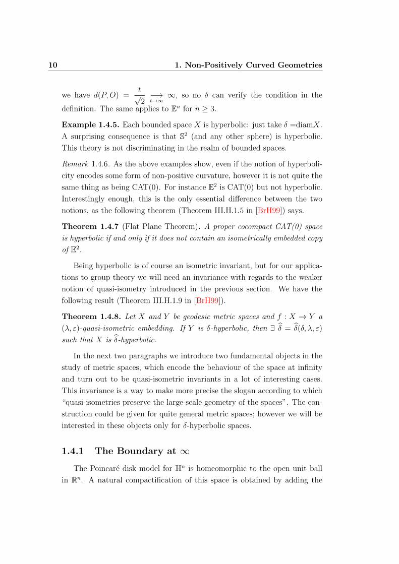
10 1. Non-Positively Curved Geometries
we have d(P,O) =t√2−→t→∞
∞, so no δ can verify the condition in the
definition. The same applies to En for n ≥ 3.
Example 1.4.5. Each bounded space X is hyperbolic: just take δ =diamX.
A surprising consequence is that S2 (and any other sphere) is hyperbolic.
This theory is not discriminating in the realm of bounded spaces.
Remark 1.4.6. As the above examples show, even if the notion of hyperboli-
city encodes some form of non-positive curvature, however it is not quite the
same thing as being CAT(0). For instance E2 is CAT(0) but not hyperbolic.
Interestingly enough, this is the only essential difference between the two
notions, as the following theorem (Theorem III.H.1.5 in [BrH99]) says.
Theorem 1.4.7 (Flat Plane Theorem). A proper cocompact CAT(0) space
is hyperbolic if and only if it does not contain an isometrically embedded copy
of E2.
Being hyperbolic is of course an isometric invariant, but for our applica-
tions to group theory we will need an invariance with regards to the weaker
notion of quasi-isometry introduced in the previous section. We have the
following result (Theorem III.H.1.9 in [BrH99]).
Theorem 1.4.8. Let X and Y be geodesic metric spaces and f : X → Y a
(λ, ε)-quasi-isometric embedding. If Y is δ-hyperbolic, then ∃ δ = δ(δ, λ, ε)
such that X is δ-hyperbolic.
In the next two paragraphs we introduce two fundamental objects in the
study of metric spaces, which encode the behaviour of the space at infinity
and turn out to be quasi-isometric invariants in a lot of interesting cases.
This invariance is a way to make more precise the slogan according to which
“quasi-isometries preserve the large-scale geometry of the spaces”. The con-
struction could be given for quite general metric spaces; however we will be
interested in these objects only for δ-hyperbolic spaces.
1.4.1 The Boundary at ∞
The Poincare disk model for Hn is homeomorphic to the open unit ball
in Rn. A natural compactification of this space is obtained by adding the
1.4 δ-Hyperbolicity 11
boundary sphere Sn−1. This is a fundamental property of classical hyperbolic
geometry: for example it provides ideal triangles and a smart way to classify
hyperbolic isometries.
It turns out that this feature does not rely on the particular homeorphism
with euclidean ball, but is an intrinsic property of the non-positive curved
geometry of Hn. Here we describe a generalization of this phenomenon to
general δ-hyperbolic spaces.
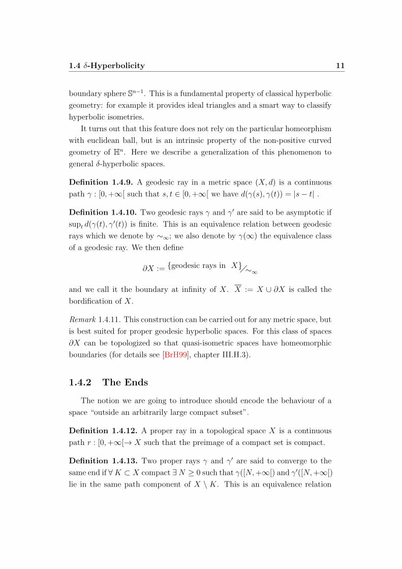
Definition 1.4.9. A geodesic ray in a metric space (X, d) is a continuous
path γ : [0,+∞[ such that s, t ∈ [0,+∞[ we have d(γ(s), γ(t)) = |s− t| .
Definition 1.4.10. Two geodesic rays γ and γ′ are said to be asymptotic if
supt d(γ(t), γ′(t)) is finite. This is an equivalence relation between geodesic
rays which we denote by ∼∞; we also denote by γ(∞) the equivalence class
of a geodesic ray. We then define
∂X := {geodesic rays in X}�∼∞
and we call it the boundary at infinity of X. X := X ∪ ∂X is called the
bordification of X.
Remark 1.4.11. This construction can be carried out for any metric space, but
is best suited for proper geodesic hyperbolic spaces. For this class of spaces
∂X can be topologized so that quasi-isometric spaces have homeomorphic
boundaries (for details see [BrH99], chapter III.H.3).
1.4.2 The Ends
The notion we are going to introduce should encode the behaviour of a
space “outside an arbitrarily large compact subset”.
Definition 1.4.12. A proper ray in a topological space X is a continuous
path r : [0,+∞[→ X such that the preimage of a compact set is compact.
Definition 1.4.13. Two proper rays γ and γ′ are said to converge to the
same end if ∀K ⊂ X compact ∃N ≥ 0 such that γ([N,+∞[) and γ′([N,+∞[)
lie in the same path component of X \ K. This is an equivalence relation
12 1. Non-Positively Curved Geometries
between proper rays which we denote by ∼end; we also denote by end(γ) the
equivalence class of a proper ray. We then define
Ends(X) := {proper rays in X}�∼end
and we call it the space of ends of X. We denote by e(X) its cardinality.
This set is usually topologized by defining a notion of convergence for
ends.
Definition 1.4.14. We say that end(γn) converges to end(γ) for n→∞ if for
every compact K ⊂ X we can find integers Nn ≥ 0 such that γn([Nn,+∞[)
and γ([Nn,+∞[) lie in the same path component of X \ K, at least for n
large enough.
We then have the following result (see Proposition I.8.29 in [BrH99]).
Theorem 1.4.15. Any quasi-isometry f : X → Y between proper geodesic
spaces induces an homeomorphism fend : Ends(X)→ Ends(Y ).
The manifest analogy between the construction of the boundary at infinity
and the space of ends is not accidental. Of course asymptotic rays converge
to the same end. Indeed one has the following result.
Proposition 1.4.16. Let X be a geodesic proper hyperbolic space. The map
∂X → Ends(X) is continuous and the fibers are the connected components
of ∂X.
Chapter 2
The Geometric and Topological
Approach to Group Theory
From an historical point of view, group theory has found in the many
branches of geometry one of the main sources of examples and ideas. But
groups are traditionally studied as abstract structures and groups arising in
geometry and topology are usually considered “just” particular examples.
On the contrary, it can be shown that every group has geometric essence,
even if it is given in purely abstract terms.
The aim of this chapter is to give the previous sentence some precise
meaning, for example showing that every group can be realized as a group of
isometries of a suitable metric space, or as the fundamental group of a suitable
topological space. The study of algebraic properties of groups through the
geometric properties of these spaces is known as Geometric Group Theory.
We present the main tools and results of this theory. In the end we
discuss a special class of groups introduced by Gromov in the 1980’s which
have given a huge boost to the theory and are also of great interest in the
study of low-dimensional manifolds.
13
14 2. The Geometric and Topological Approach to Group Theory
2.1 Groups as Fundamental Groups
Throughout this chapter let G be a group and fix some finite presentation
G = 〈gα|rβ〉. It is well known that every group has a presentation (e.g. it
is isomorphic to a quotient of the free group over itself), but this is quite
trivial and useless. Even if some aspects of the theory apply to the general
setting, in the following we consider only finitely presented groups, since this
is the class of groups that arise in the study of low-dimensional manifolds
and which we will be concerned with.
In this section we construct some topological spaces with fundamental
group isomorphic to G and derive some results that will be useful in the
following chapters.
2.1.1 Presentation Complex
Let X be a connected 1-dimensional CW complex. Then π1(X) is a free
group. Suppose we attach a 2-cell via some attaching map ϕ : S1 → X
and we call the resulting space Y ; we have a natural inclusion X ↪→ Y . Of
course ϕ(S1) gives a loop in Y and a standard application1 of Seifert-van
Kampen theorem shows that π1(Y ) ∼= π1(X)�N(ϕ(S1)), where N(ϕ(S1)) is
the normal closure of ϕ(S1) in π1(X).
In other words, attaching 2-cells to a graph introduces relations in its
fundamental group. This allows us to prove the following theorem.
Theorem 2.1.1. Every group G is the fundamental group of a finite 2-
dimensional CW complex.
Proof. Let G = 〈gα|rβ〉 be a presentation of G. Let X be a bouquet of
oriented circles, one for each gα. Each relation rβ is a finite word in these
generators (and their inverses) as rβ = g±1α1. . . g±1
αp. Then we glue a 2-cell e2
β
via an attaching map defined in this way: subdivide the boundary of e2β in p
edges a1 . . . ap and send ai to the loop labelled g±1αi
(where g−1αi
is just gαiwith
the opposite orientation). Do this for each relation and call XG the resulting
space. From the previous discussion it follows that π1(XG) ∼= G.
1For a detailed proof see Proposition 1.26 in [Hat02].

2.1 Groups as Fundamental Groups 15
Definition 2.1.2. The complex XG constructed in the previous proof is
called the Presentation Complex associated to the presentation G = 〈gα|rβ〉of G.
Example 2.1.3. Let G be a cyclic group of order n; a presentation is given
by G = 〈g|gn〉, so XG is obtained from a circle by glueing a disk via a map
whose restriction to the boundary is a map of degree n. For example for
n = 2 we get XG∼= RP2. But for n ≥ 3 we never get a smooth surface.
Remark 2.1.4. The previous example shows that in general we cannot expect
XG to be locally euclidean, i.e. to be a topological manifold. For the sake of
completeness, we report the following result, which says that if you accept
to pay some extra dimension then you can always realize G in a nicer way.
Theorem 2.1.5. Every finitely presented group G is the fundamental group
of a 4-dimensional compact connected smooth manifold.
This theorem, combined with the undecidability of the Isomorphism Prob-
lem for groups, is the reason why manifolds of dimension n ≥ 4 cannot be
effectively classified. The same theorem is false in dimension 3.
The following example shows a key feature of this theory: groups that
look strange from a purely algebraic point of view, may have a quite simple
presentation complex which encodes a lot of extra structure, which may be
at first not visible in the combinatorial data of a presentation.
Example 2.1.6. Let G = 〈a1, b1 . . . , a2n, b2n|∏n
i=1[ai, bi]〉. Then XG is the
closed orientable surface of genus n. This follows from the fact that such a
surface can be obtained by glueing the edges a regular polygon with 4n edges
(in R2 if n = 2 or H2 if n ≥ 3).
Remark 2.1.7. One can ask whether the complex XG, that a priori depends
on the chosen presentation, is actually an invariant of G. The answer turns
out to be no in a rather strong sense: presentation complexes associated to
different presentations of G can even be not homotopically equivalent, as the
following example shows.
16 2. The Geometric and Topological Approach to Group Theory
Example 2.1.8. Let G be the trivial group; a presentation is given by G =
〈∅|∅〉 and the associated complex is just a point. ButG can also be presented
by G = 〈a|a, a−1〉, and the complex associated to this presentation is S2.
For now, we content ourselves with the following result which gives a par-
tial answer to the question of how much a group G determines the complexes
XG associated to different presentations. See Proposition 1B.9 in [Hat02] for
a proof.
Theorem 2.1.9. Let f : G → H be a homomorphism of groups. Then we
can find a presentation complex associated to some presentation of each group
and a map ϕ : XG → XH such that f = π1(ϕ).
The point is that the map ϕ will not in general be unique, and this let
different presentations give non homotopically equivalent complexes. The
next section deals with this problem.
2.1.2 Eilenberg-MacLane Spaces
In this section we refine the construction of the presentation complex to
achieve better results.
Definition 2.1.10. Let G be a group. An Eilenberg-MacLane space for G is
a path connected topological space X with contractible universal cover and
such that π1(X) = G. We also say that X is a K(G, 1).
Remark 2.1.11. From the long exact sequence associated to the universal
covering map, we see that in particular all higher homotopy groups are trivial.
So a K(G, 1) is nicer than a presentation complex from the point of view of
homotopy theory, since all the higher dimensional homotopy has been killed;
on the other hand we pay our debt with the fact that typically a K(G, 1)
has a cell structure with cell in high dimensions (even in infinitely many
dimensions sometimes).
Example 2.1.12. S1 is a K(Z, 1) and more generally a graph is a K(G, 1)
for G a free group, since the universal cover is a tree.
2.1 Groups as Fundamental Groups 17
Example 2.1.13. A closed hyperbolic surface S is a K(π1(S), 1), because
its universal cover is H2. The same is true for higher dimensional closed
hyperbolic manifolds.
Example 2.1.14. In the previous section we have seen S2 and RP2 arising as
presentation complexes. They are not K(G, 1) for their fundamental groups.
Remark 2.1.15. It can be proved that every group admits a K(G, 1), for ex-
ample by attaching higher dimensional cells to any presentation complex for
G; however the general construction produces infinite dimensional complexes
even if G admits some easier K(G, 1), as in the case of Z. In the following
we will not need this full generality, since we will be able to find K(G, 1) “by
hands”.
The main reason to switch from presentation complexes to Eilenberg-
MacLane spaces is the fact that they are homotopically rigid, i.e. do not
show the ambiguity of example 2.1.8. We have a result analogous to Theorem
2.1.9 but enriched by a universal property which guarantees uniqueness.
Theorem 2.1.16. Let X be a connected CW complex, Y a K(G, 1) and f :
π1(X, x0) → π1(Y, y0) = G a homomorphism. Then ∃ ϕ : (X, x0) → (Y, y0),
which is unique up to homotopy relative to the basepoint.
A proof of this result is available in [Hat02]. It is then easy to prove that:
Corollary 2.1.17. The homotopy type of a CW complex K(G, 1) is determ-
ined by G.
Proof. Let X, Y be two K(G, 1) with a CW complex structure; their fun-
damental groups are thus isomorphic (and both isomorphic to G). Let
f : π1(X, x0) → π1(Y, y0) and g : π1(Y, y0) → π1(X, x0) a couple of in-
verse homomorphisms (i.e. f = g−1 and vice versa). The previous theorem
gives a pair of maps ϕ : (X, x0)→ (Y, y0) and ψ : (X, x0)→ (Y, y0) inducing
f and g respectively. But then ϕψ and ψϕ induce the identity on the fun-
damental groups and so (again by the theorem) are homotopic (relatively to
basepoints) to the identities on each space. Thus ϕ and ψ give a homotopy
equivalence between X and Y .
18 2. The Geometric and Topological Approach to Group Theory
We now want to discuss two applications of the previous constructions:
the first is mainly algebraic, whereas the second is of geometric interest.
Remark 2.1.18. The previous result gives a smart way to carry the whole
machinery of homological algebra from the category of topological spaces to
that of groups: just define the (co)homology groups of a group G to be the
(co)homology groups of any K(G, 1):
Hi(G) := Hi(K(G, 1))
H i(G) := H i(K(G, 1))
this is well-posed since all K(G, 1) are homotopy equivalent. This turns out
to be equivalent to the algebraic approach to group (co)homology via Tor
and Ext functors.
Remark 2.1.19. The other application is about the connection between ho-
motopy and cohomology of CW complexes. Let X, Y be CW complexes and
〈X, Y 〉 denote the set (no additional structure is involved here) of basepoint-
preserving homotopy classes of maps X → Y . A classical result in algebraic
topology (see e.g. Theorem 4.57 in [Hat02]) states that for any abelian group
G there is a canonical bijection (of sets)
〈X,K(G, 1)〉 ←→ H1(X,G)
where H1(X,G) denotes singular cohomology with coefficients in G. The
case G = Z is really nice: here we can take S1 as K(G, 1) and obtain the
bijection
〈X,S1〉 ←→ H1(X)
Now clearly every map X → S1 induces a morphism π1(X) → Z. But
since S1 is a K(Z, 1) the theorem says that the converse is also true, that
is every morphism π1(X) → Z is induced by a map X → S1 unique up to
basepoint-preserving homotopy. This gives a bijection
H1(X)←→ 〈X,S1〉 ←→ Hom(π1(X),Z)
that we will exploit in the following chapters.

2.2 Groups as Isometry Groups 19
2.2 Groups as Isometry Groups
In this section we introduce spaces which have a more geometric flavour:
they come equipped with natural metrics and isometric G-actions.
2.2.1 Cayley Graph
Let S be a fixed set of generators for G.
Definition 2.2.1. The Cayley Graph associated to G and to S is the graph
Cay(G,S) defined in this way:
• the vertices of Cay(G,S) are the elements of G;
• two vertices x, y ∈ G span an edge if and only if ∃ s ∈ S such that
y = xs; in this case we label this edge by s and orient it from x to y.
Remark 2.2.2. We usually want S to be closed under inversion, so that we
can just speak of “words in the generators” instead of having to consider
“words in the generators and their inverses”. Anyway this can produce some
redundancy in the construction of the Cayley graph; we adopt the following
conventions:
• If e ∈ S (where e denotes the identity of G), then we get a trivial loop
at each point, which we agree to erase.
• When s, s−1 ∈ S, for each g ∈ G we get an edge labelled s from g
to gs and an edge labelled s−1 from gs to g; they of course carry the
same information, so we draw just one of them. This amounts to make
a choice of one generator for each couple s, s−1 ∈ S (notice that this
works only if s 6= s−1); any such choice gives the same (undirected)
graph.
• If some generator has order 2 (i.e. s = s−1), then the previous choice
cannot be done: in this case we agree to represent it as an undirected
edge .
With these conventions, adding to a set of generators the inverses of its
elements (as well as the identity), does not change the resulting Cayley graph
(as long as we do not care about orientations of the edges).
20 2. The Geometric and Topological Approach to Group Theory
Remark 2.2.3. Cay(G,S) is a connected graph with 0-skeleton identified with
G itself and there is a natural action of G on Cay(G,S)0 given by left mul-
tiplication
G× Cay(G)0 → Cay(G)0, g, x 7→ gx
This action is free and transitive on Cay(G,S)0 and can be extended to a
simplicial action to the 1-cells by setting
g, [x, xs] 7→ [gx, gxs]
If the generating set is finite, the action is also cocompact, i.e. ∃ K ⊂Cay(G,S) compact such that G.K = Cay(G,S); namely K is given by ver-
tices corresponding to the identity of G and the generators in S together with
all edges between them; equivalently, the quotient Cay(G,S)�G is a compact
complex.
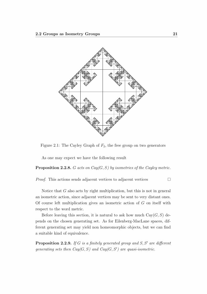
Example 2.2.4. When the standard generating sets are understood, Cay(Zn)
is just a loop subdivided in n arcs, Cay(Zn) is the integer lattice in Rn and,
if G = Fn is the free group on n generators, then Cay(G) is the tree in which
each vertex has 2n outgoing edges.
There is a standard way to turn a graph into a metric space, just setting
the length of each edge.
Definition 2.2.5. The Cayley metric dS on Cay(G,S) is obtained declaring
each edge isometric to the unit interval [0, 1] ⊂ R and then considering the
path-metric.
Remark 2.2.6. There is a correspondence between edge-paths in Cay(G,S)
and words inG (with respect to the generating set S), since edges of Cay(G,S)
are labelled by generators of G. The nice thing about the Cayley metric is
that for each g ∈ G the length of the shortest word representing g in the
generators in S equals the distance dS(g, e) of g from the identity element in
the Cayley graph associated to the generating set S.
Definition 2.2.7. The word metric on G (with respect to the generating
set S) is defined to be the restriction of the Cayley metric to the vertex set,
which is identified with G by construction. In this way G itself is turned into
a metric space.
2.2 Groups as Isometry Groups 21
Figure 2.1: The Cayley Graph of F2, the free group on two generators
As one may expect we have the following result
Proposition 2.2.8. G acts on Cay(G,S) by isometries of the Cayley metric.
Proof. This actions sends adjacent vertices to adjacent vertices
Notice that G also acts by right multiplication, but this is not in general
an isometric action, since adjacent vertices may be sent to very distant ones.
Of course left multiplication gives an isometric action of G on itself with
respect to the word metric.
Before leaving this section, it is natural to ask how much Cay(G,S) de-
pends on the chosen generating set. As for Eilenberg-MacLane spaces, dif-
ferent generating set may yield non homeomorphic objects, but we can find
a suitable kind of equivalence.
Proposition 2.2.9. If G is a finitely generated group and S, S ′ are different
generating sets then Cay(G,S) and Cay(G,S ′) are quasi-isometric.
22 2. The Geometric and Topological Approach to Group Theory
Proof. Here we consider four metric spaces: (Cay(G,S),d), (Cay(G,S ′),d′),
(G, d) and (G, d′), that is the two Cayley graphs with their word metrics and
the two metric spaces obtained from G itself equipped with the respective
word metrics. The inclusion of (G, d) into (Cay(G,S),d) is a quasi-isometric
embedding (it is an isometric embedding indeed); moreover by the definition
of the Cayley metric, each point in (Cay(G,S),d) lies in the 12-neighbourhood
of the 0-skeleton (which is identified with G itself), therefore the inclusion
is indeed a quasi-isometry. From the discussion in 1.3, it is then enough to
show that (G, d) and (G, d′) are quasi-isometric.
Each generator si ∈ S can be written as a word in S ′. Let li denote
the minimal length of such a word and let K1 := max li, which is well
posed since S is finite. It is then clear from the previous discussion that
dS′(g, e) ≤ K1dS(g, e). Exchanging the roles of S and S ′ define K2 and ob-
tain dS(g, e) ≤ K2dS′(g, e). Finally set K := max{K1, K2}. This proves that
the identity map on G induces a (K, 0)-quasi-isometry between (G, d) and
(G, d′) (which is actually a bilipschitz equivalence, i.e. we do not need any
additive constant).
Remark 2.2.10. It follows from the previous proof that each group has an
associated metric space well-defined only up to quasi-isometry, i.e. a quasi-
isometry type. This is the right thing to consider, since we cannot expect
to obtain an isometry type in general, as the following example shows in a
quite dramatic way.
Example 2.2.11. Consider the group of integers Z; this is naturally gener-
ated by 1. As discussed in the example 2.2.4, the Cayley graph associated to
this generating set is an infinite chain, which we can identify with the real
line (compare also example 1.3.3).
0 1 2 3 4 5 6+1 +1 +1 +1 +1 +1
Figure 2.2: (A portion of) the Cayley Graph of Z with respect to {1}
But we can as well generate Z with {2, 3} (or with any other couple
of coprime numbers by Bezout’s Identity), and this would give a strongly

2.2 Groups as Isometry Groups 23
different Cayley graph; the next picture shows an example of a portion of
what we would get.
0
2 4
6
3
15
+2
+3
+2
+2
+3
+2
+3+3
+2
Figure 2.3: (A portion of) the Cayley Graph of Z with respect to {2, 3}
As you can see we get closed loops, which exemplifies the fact that graphs
arising from different presentation can not only be non isometric, but even
not homotopy equivalent. One of the main features of the notion of quasi-
isometry is that it does not require continuity.
2.2.2 Cayley Complex
In the constructions of the previous section we have focused on the gen-
erating part of a presentation of G, neglecting relations; now we want to
incorporate them into this construction. This will lead to a connection to
presentation complexes.
Let G = 〈S|R〉 = 〈s1, . . . , sn|r1, . . . , rp〉 be a presentation for G and
Cay(G,S) the associated Cayley graph. The relations in R give rise to loops
in Cay(G,S) which give generators for π1 (Cay(G,S)). We want to make
these loops nullhomotopic to obtain a simply connected complex with a nice
G-action and which still contains Cay(G,S) as a subcomplex. To do this we
can glue a 2-cell along each of these loops. This certainly yields a simply
connected complex with a natural G-action obtained extending the action
on Cay(G,S) in a cellular way, but the action is not nice enough, as the
following example shows.
24 2. The Geometric and Topological Approach to Group Theory
Example 2.2.12. Take Zn = 〈g|gn〉. Then the above construction gives
a complex which has one 2-cell with the boundary divided into n arcs (it
is just Cay(Zn, {[1]})). The action of Zn on the boundary is by rotations,
therefore the extension to the complex is not free because it fixes some point
in the interior of the cell. The general situation of a non-free action is not so
different: if we have a non trivial stabilizer of some inner point of a 2-cell,
then its action always induces a permutation of the boundary vertices and
so the action on the whole cell is that of a dihedral group.
One way to avoid this problem is to consider that each relation gives a
loop based at any vertex of Cay(G,S) and to glue a 2-cell to each of these
loops. In this way, whenever we see a loop of length k we actually consider
k different loops based at the k different vertices on the loops and glue k
different 2-cells identifying their boundaries in Cay(G,S). When we act with
an element that stabilizes the loop, the action on the boundary is the one
described above, but in the interior we go from one cell to another. In this
way we remove fixed points.
Definition 2.2.13. The 2-complex obtained by the above construction is
called the Cayley complex associated to the presentation G = 〈S|R〉.
Example 2.2.14. Take Zn = 〈g|gn〉. The Cayley complex is obtained by n
copies of the unit disk glued along their boundaries, which come equipped
with a subdivision in n arcs which descend to an analogous subdivision of
the unique boundary in the quotient. The action of g sends a cell to another
cell after a rotation of2π
n. For example for n = 2 this is just the covering
map S2 → RP2 = XZ2 . Notice that if we glue just one cell to Cay(Z2, {[1]})then we get a disk (not a sphere) and the quotient map is not a covering map
since it has a cone singularity of order 2 at the origin.
The situation described in the previous example is quite general.
Proposition 2.2.15. The Cayley complex is the universal cover of the pre-
sentation complex XG associated to the same presentation of G.
Proof. The above discussion proves that the action of G on this complex is
free and properly discontinuous, and the orbit space is just XG; thus it is a
2.3 Hyperbolic Groups 25
covering space of XG. Moreover it is simply connected by construction, so it
is the universal cover.
We now quote the following theorem by Nielsen and Schreier, which shows
an example of the way in which algebraic properties can be deduced from ge-
ometric and topological considerations about the spaces we have constructed
in this chapter.
Theorem 2.2.16. A subgroup H of a free group G is free.
Proof. Take XG as a bouquet of circles. Since no relations are involved the
universal cover is just the tree Cay(G). A subgroup H of G is associated
to an intermediate covering space Cay(G)→ YH → XG. But then YH is
necessarily a graph, so H = π1(YH) must be free.
2.3 Hyperbolic Groups
As an application to the material presented so far, we present a class
of groups introduced by Gromov in [Gro87] which happens to be of great
interest in low-dimensional topology as we will see in the last chapter.
Definition 2.3.1. A finitely generated group G is hyperbolic (also Gromov-
hyperbolic or word-hyperbolic) if its Cayley graph with respect to some gen-
erating set is δ-hyperbolic (fore some δ) when equipped with the Cayley
metric.
Remark 2.3.2. Notice that this definition does not depend on the choice of
the generating set, but the precise value of δ does. Indeed from 2.2.9 we
know that Cayley graphs with respect to different generating set are quasi-
isometric and from 1.4.8 we know that being hyperbolic is a quasi-isometric
invariant.
Example 2.3.3. From the examples in 1.4.2 and 2.2.4 we readily have that
• finite groups and free groups are hyperbolic;
• free abelian groups are not hyperbolic;
• any group with a subgroup isomorphic to Z⊕Z cannot be hyperbolic.
26 2. The Geometric and Topological Approach to Group Theory
The last example is quite significant and motivates the following criterion,
which will be useful in later chapters.
Theorem 2.3.4. Let G be a group acting properly and cocompactly by iso-
metries on a CAT(0) space X. Then G is hyperbolic if and only if X does
not contain an isometrically embedded copy of E2.
This is Theorem III.Γ.3.1 in [BrH99], which we refer to for details. Notice
the analogy with the Flat Plane Theorem (see 1.4.7).
Remark 2.3.5. From what we have said so far, it follows that every group is a
quasi-isometric type of geodesic metric spaces. G is hyperbolic if and only if
this quasi-isometric type is hyperbolic. In 1.4.1 we have constructed a bound-
ary at infinity for hyperbolic spaces and said that quasi-isometric proper
geodesic spaces have homeomorphic boundary (with respect to some suitable
topology). As a result we can unambiguously talk about the boundary at
infinity ∂G of a hyperbolic group G; notice that the Cayley graphs associated
to a finitely generated group are proper metric spaces, since the unit ball
centered at the origin has finitely many vertices. The same reasoning of
course applies to the space of ends introduced in 1.4.2, therefore the following
definition is well posed.
Definition 2.3.6. Let G a hyperbolic group. We define the boundary at
infinity of G and the space of ends of G to be
∂G := ∂Cay(G,S) and Ends(G) := Ends(Cay(G,S))
for some (finite) generating set S. We also define e(G) as the cardinality of
Ends(G).

Chapter 3
Special Cube Complexes
The aim of this chapter is to introduce a class of CW complexes which
have proved really useful in the study of 3-manifolds, since they provide a
smart way of embedding fundamental groups into well-organized groups. The
standard reference for the whole material is taken from [HaW08], with the
exception of the proof of Theorem 3.3.8 which has been made self-contained,
avoiding any appeal to the metric properties of these complexes. A discussion
of the original approach is given in the last section.
3.1 Hyperplanes and Walls in Cube Complexes
Let I denote the interval [−1, 1] ⊂ R and In its n-fold cartesian power,
which we call n-cube.
Definition 3.1.1. A cube complex is a CW complex which is obtained by
glueing cubes via isometries of their faces. In other words, the attaching
map of each n-cell (i.e. n-cube) is defined on ∂In and its restriction to an
(n− 1)-face of ∂In is given by an isometry of that face with In−1 composed
with an (n− 1)-cell of X.
Remark 3.1.2. Notice that this definition allows two n-cells to be glued along
two arbitrary faces (which are not necessarily 1-codimensional), as long as
they have the same dimension; for example we can glue two squares at one
point or along an edge. We can also assemble a square and a segment by
27

28 3. Special Cube Complexes
Figure 3.1: A cube complex
identifying two points in their 0-skeleton; this allows for complexes which
may have different local maximal dimension in different points, i.e. we can
have one point which is contained in a n-dimensional cell and another point
such that each cell which contains it has dimension k < n. Another thing to
observe is that we do not require the attaching maps to be injective on the
boundary of the cubes; for example an n-torus is a cube complex: this can
be seen considering it as a quotient of In in the usual way.
The main feature of cube complexes is the availability of canonical sub-
complexes of (local) codimension 1, which we now define.
Definition 3.1.3. A midcube of In is a subspace of the form M = {x ∈In | xi = 0} for some i and the edges of In which are orthogonal to it are
called its dual edges.
Figure 3.2: Midcubes in I2 and I3
Remark 3.1.4. The crucial properties of midcubes are the following

3.1 Hyperplanes and Walls in Cube Complexes 29
• if a midcube M ⊂ In intersects a (n− 1)-face F ⊂ In, then the inter-
section M ∩ F is a midcube N of F ;
• vice versa, for each midcube N in a (n − 1)-face F ⊂ In there is a
unique midcube M ⊂ In such that M ∩ F = N ; this means there is a
unique way to extend a midcube of a face to a midcube of the whole
cube.
By induction on the dimension of the cells, the previous properties hold for
any face of the cube, not necessarily 1-codimensional.
This allows us to propagate in a canonical way a midcube of a cell to
adjacent cells; notice that this property does not hold in simplicial complexes.
What is obtained after a “maximal propagation” is a locally 1-codimensional
subspace, which can be thought of as a “hypersurface” inside X or, as we
will say, a hyperplane. But we want an abstract way to define these objects.
Definition 3.1.5. Given a cube complexX we construct a new cube complex
H(X), called hyperplane complex of X, as follows: the n-cubes of H(X) are
midcubes of the (n + 1)-cubes of X and the attaching maps in H(X) are
obtained in the obvious way by restriction of those of X to midcubes. A
hyperplane of X is by definition a connected component of H(X).
Figure 3.3: A hyperplane in a cube complex
30 3. Special Cube Complexes
Being locally 1-codimensional allows hyperplanes to be identified with
their 1-dimensional complement; this gives rise to a fundamental duality in
a cube complex, which we know describe.
Definition 3.1.6. Let X be a cube complex.
• An edge a ∈ X1 is said to be dual to an hyperplane H of X if its
midpoint is a vertex of H (in H(X)); this is equivalent to saying that
H intersects a (in X).
• Two edges of X are said to be elementary parallel if they appear as
opposite edges of a square. We call parallelism the equivalence relation
among edges of X generated by elementary parallelisms. If a ∈ X1, its
parallelism class is denoted W (a) and called the wall through a.
The following proposition establishes the desired duality.
Proposition 3.1.7. There is a bijective correspondence between hyperplanes
and walls of X, obtained associating at each hyperplane the set of dual edges
and to each wall the unique hyperplane to wich it is dual.
The uniqueness in the previous proposition is guaranteed by the fact
(stressed above) that it is possible to extend midcubes in a unique way from
a cube to the adjacent ones. This result is very useful, since it allows to
translate conditions about the hyperplanes about conditions about the walls,
which live only in the 2-skeleton of X and are thus easier to deal with in
proofs.
We need just one more technical definition.
Definition 3.1.8. The link of a point v in a cube complex X is the complex
lk(v,X) obtained by taking a point for each edge that contains the point
and in which k + 1 points span a k-simplex if and only if there is a cube
of dimension k + 1 which contains the corresponding edges in its boundary.
A geometric realization of this complex is given by intersecting the cube
complex with a small sphere centered at the point v.
In general the link of a vertex carries only the structure of a CW-complex.
Definition 3.1.9. A cube complex is simple if the link of each vertex is a
simplicial complex.
3.2 Speciality Conditions 31
This in particular means that two squares cannot meet in a pair of consec-
utive edges, because otherwise we would see a bigon in the link of the vertex
in the middle, which is forbidden in the definition of simplicial complex. We
will consider only simple cube complexes in the following.
3.2 Speciality Conditions
We now turn our interest to a class of cube complexes in which a few
kinds of pathologies are forbidden. These pathologies are about the way
hyperplanes are immersed in the complex; it will be useful to have a definition
in term of hyperplanes themselves and a dual one about walls.
Definition 3.2.1. Let X be a cube complex, H,K two hyperplanes in X
and W,Z their dual walls. We say that:
1. H selfintersects if it contains at least two midcubes from the same cube
of X. Equivalently there are two edges of W which appear as adjacent
edges of some square of X. H is said to be embedded if it does not
selfintersect. We also say that a wall is selfintersecting or embedded if
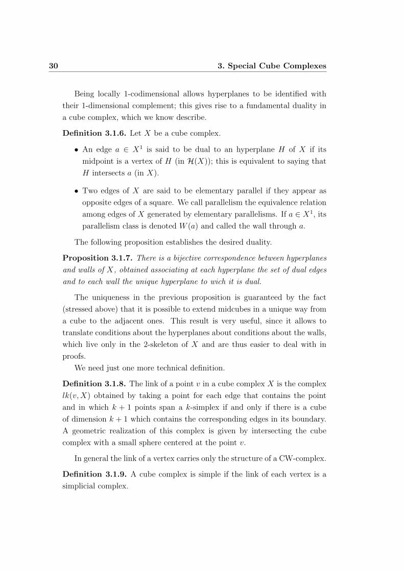
its dual hyperplane is selfintersecting or embedded.
Figure 3.4: A selfintersecting hyperplane
2. An embedded hyperplane H is 2-sided if its normal bundle (i.e. the
union of open cubes which contain the midcubes of H) is trivial, that
is isomorphic to H×I. Equivalently it is possibble to orient coherently
all the edges of W .

32 3. Special Cube Complexes
Figure 3.5: A 1-sided hyperplane
3. H and K osculate if “their normal bundle are tangent”; more precisely,
we say H and K osculate at (v, a, b) if a ∈ W , b ∈ Z and they intersect
at the vertex v ∈ X, but there is no cube of X that contains both a
and b (otherwise this would give a configuration of intersection). If H
and K are 2-sided, the osculation is said to be direct or indirect if the
orientations induced on v respectively agree or disagree. We also say
that H selfosculates at (v, a, b) if a, b ∈ W and they intersect at the
vertex v ∈ X, but there is no cube of X that contains both a and b
(otherwise this would give a configuration of selfintersection); as before
we distinguish between direct and indirect selfosculation according to
how orientations are induced on the common point.
Figure 3.6: A directly selfosculating hyperplane (left) and an indirectly self-
osculating hyperplane (right)
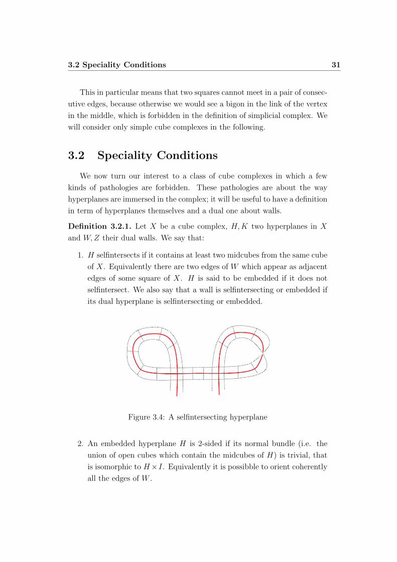
4. H and K inter-osculate if there is a cube in which they intersect and a
3.2 Speciality Conditions 33
point (not in that cube) in which they osculate (without intersecting).
Figure 3.7: A pair of interosculating hyperplanes
We now are ready to give the main definition.
Definition 3.2.2. Let X be a cube complex. Then
• X is special if it is simple, each hyperplane is embedded and non di-
rectly selfosculating and there are no interosculating hyperplanes;
• X is A-special it is special and if each hyperplane is 2-sided.
Remark 3.2.3. Notice that since all the speciality conditions can be expressed
in terms of edges and squares, everything here depends only on the 2-skeleton
of X. Therefore X is (A-)special if and only if X2 is (A-)special.
Remark 3.2.4. We give these two different definitions since we will associate
to a closed hyperbolic 3-manifold a cube complex which in general is just
special, but the theory of cube complexes needs A-speciality to express all of
its power. We will see that, in a suitable sense, A-speciality can always be
recovered from speciality alone.
3.2.1 Virtual Equivalence
In this section we prove the equivalence of the speciality conditions up to
finite covers.

34 3. Special Cube Complexes
Definition 3.2.5. Let X, Y be simple cube complexes.
• A map f : X → Y is a combinatorial map if for each n-cell ϕX : In → X
there exist a n-cell ϕY : In → Y and an isometry j : In → In such that
f ◦ ϕX = ϕY ◦ j.
• A combinatorial map f : X → Y is an immersion if the maps induced
on links fv : lk(v,X)→ lk(f(v), Y ) are injective.
• An immersion f : X → Y is a local isometry if ∀ v ∈ X0 we have that
fv(lk(v,X)) is a full subcomplex of lk(f(v), Y ), i.e. if each simplex of
lk(f(v), Y ) whose vertices are in fv(lk(v,X)) is itself in fv(lk(v,X)).
Remark 3.2.6. This terminology is reminiscent of that of Riemannian geome-
try: a combinatorial immersion is something like a smooth map with injective
differential, and having full subcomplexes is something like having surjective
differential. This analogy is not accidental: it is actually possible to turn
cube complexes into nice metric spaces; our treatment could be carried out
without appealing to this fact. However the original discussion in [HaW08]
relies on this property, so we will spend a few words on it at the end of the
chapter (see 3.4).
The next lemma is about stability of the speciality conditions under com-
binatorial maps.
Lemma 3.2.7. Let f : X → Y be a combinatorial map between cube com-
plexes. Then:
1. Y has embedded (resp. 2-sided) hyperplanes ⇒ X has embedded (resp.
2-sided) hyperplanes;
2. suppose that either Y has embedded hyperplanes and f is an immersion,
or that f |X2 : X2 → Y 2 is a local isometry; then if Y has no direct
selfosculations, then the same holds for X;
3. Y has embedded hyperplanes and has no interosculations and f |X2 :
X2 → Y 2 is a local isometry ⇒ X has no interosculations.
3.2 Speciality Conditions 35
Proof. Since f is combinatorial, it sends edges and squares in X to edges
and squares in Y , so it preserves elementary parallelism and sends walls in
walls.
1. Suppose X has a wall W which selfintersects or is 2-sided; then f(W )
would be (contained in) a wall of Y which would selfintersect or be
2-sided, and this is absurd.
2. Suppose an oriented wall W of X directly selfosculates in (v,−→a ,−→b );
then in Y we have a wall V which passes through f(−→a ) and f(−→b ). Since
f is a local immersion on X2, we have f(−→a ) 6= f(−→b ); this means that
V either selfintersects or directly selfosculates in (f(v), f(−→a ), f(−→b )),
but both options are absurd under the hypothesis.
3. Let V and W be wall of X which interosculate and let (v,−→a ,−→b ) be
the configuration of osculation. The wall through f(−→a ) intersects
the one through f(−→b ), so they must be distinct; if f(−→a ) and f(
−→b )
were adjacent in lk(f(v), Y ) then −→a and−→b should be adjacent in
lk(v,X) because f is a local isometry; but this does not happen, by
definition of interosculation. Therefore the two walls of Y osculate in
(f(v), f(−→a ), f(−→b )), which is absurd.
Since a covering map is of course a local isometry, we have the following
result.
Corollary 3.2.8. Each covering complex of a special (resp. A-special) com-
plex is still special (risp. A-special).
In the proof of the next lemma we will exploit a combinatorial approach
to the homotopy properties of our cube complex.
Remark 3.2.9. We observe that, by cellular approximation, every path in
a cube complex is homotopic to an edge-path in the 1-skeleton and each
homotopy between edge-paths can be realized by a sequence of elementary
homotopies taking place in some square. Elementary homotopies (fixing
extremities) of an edge-path x1 . . . xn in a square can only take one of these
two forms:

36 3. Special Cube Complexes
1. x1 . . . xi−1xix−1i xi+1 . . . xn ' x1 . . . xi−1xi+1 . . . xn
2. x1 . . . xixj . . . xn ' x1 . . . xhxk . . . xn whenever xixjx−1k x−1
h is the (ori-
ented) perimeter of some square of X
The following result establishes the virtual equivalence (i.e. up to a finite
cover) of the two definitions of speciality.
Lemma 3.2.10. Let X be a cube complex with a finite number of walls and
with no selfintersecting walls. Then ∃ X ′ finite cover of X whose hyperplanes
are 2-sided.
Proof. Let W1, . . . ,Wn be the walls of X e let γ : [0, 1]→ X1 an edge-path.
By the previous description of elementary homotopies (fixing extremities),
the parity of intersection of γ with each Wj is preserved by these homotopies;
therefore we have a morphism λj : π1(X)→ Z2 whose kernel has finite index.
Since the number of walls is finite,
H :=n⋂j=1
ker(λj)
is a finite index subgroup, so the associated cover p : X ′ → X has finite
degree.
Now suppose there is an edge −→a of X ′ which is parallel to its opposite←−aand let {−→a = −→a 1,
−→a 2, . . . ,−→a m = ←−a } be a sequence of elementary parallel
edges which realizes the parallelism between −→a and←−a . Let Qk be the square
in which the elementary parallelism between −→a k and −→a k+1 takes place and
let−→b k the edge of Qk such that i(
−→b k) = t(−→a k) and t(
−→b k) = t(−→a k+1), where
i and t denote the initial and terminal point of an edge with respect to the
chosen orientation. In particular we have t(−→b m) = t(−→a m) = t(←−a ) = i(−→a )
which means that γ := (−→a ,−→b 1, . . . ,
−→b m) is a closed edge-path.
Then p ◦ γ ∈ H and by construction of H we have λj(p ◦ γ) = 0 for
each j = 1, . . . , n, in particular for that j such that Wj = W (p(a)); as a
consequence #({p(a), p(b1), . . . , p(bm)} ∩Wj) is even. On the other hand by
construction Wj ∩W (p(bk)) 6= ∅ and so p(bk) 6∈ Wj since X has embedded
hyperplanes and this implies that ({p(a), p(b1), . . . , p(bm)} ∩Wj) = {p(a)}.This is absurd because it should have an even number of elements.
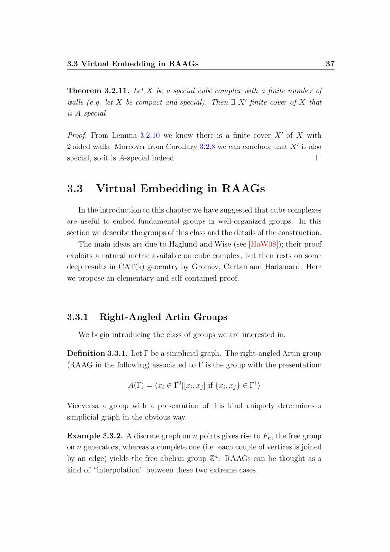
3.3 Virtual Embedding in RAAGs 37
Theorem 3.2.11. Let X be a special cube complex with a finite number of
walls (e.g. let X be compact and special). Then ∃ X ′ finite cover of X that
is A-special.
Proof. From Lemma 3.2.10 we know there is a finite cover X ′ of X with
2-sided walls. Moreover from Corollary 3.2.8 we can conclude that X ′ is also
special, so it is A-special indeed.
3.3 Virtual Embedding in RAAGs
In the introduction to this chapter we have suggested that cube complexes
are useful to embed fundamental groups in well-organized groups. In this
section we describe the groups of this class and the details of the construction.
The main ideas are due to Haglund and Wise (see [HaW08]); their proof
exploits a natural metric available on cube complex, but then rests on some
deep results in CAT(k) geoemtry by Gromov, Cartan and Hadamard. Here
we propose an elementary and self contained proof.
3.3.1 Right-Angled Artin Groups
We begin introducing the class of groups we are interested in.
Definition 3.3.1. Let Γ be a simplicial graph. The right-angled Artin group
(RAAG in the following) associated to Γ is the group with the presentation:
A(Γ) = 〈xi ∈ Γ0|[xi, xj] if {xi, xj} ∈ Γ1〉
Viceversa a group with a presentation of this kind uniquely determines a
simplicial graph in the obvious way.
Example 3.3.2. A discrete graph on n points gives rise to Fn, the free group
on n generators, whereas a complete one (i.e. each couple of vertices is joined
by an edge) yields the free abelian group Zn. RAAGs can be thought as a
kind of “interpolation” between these two extreme cases.
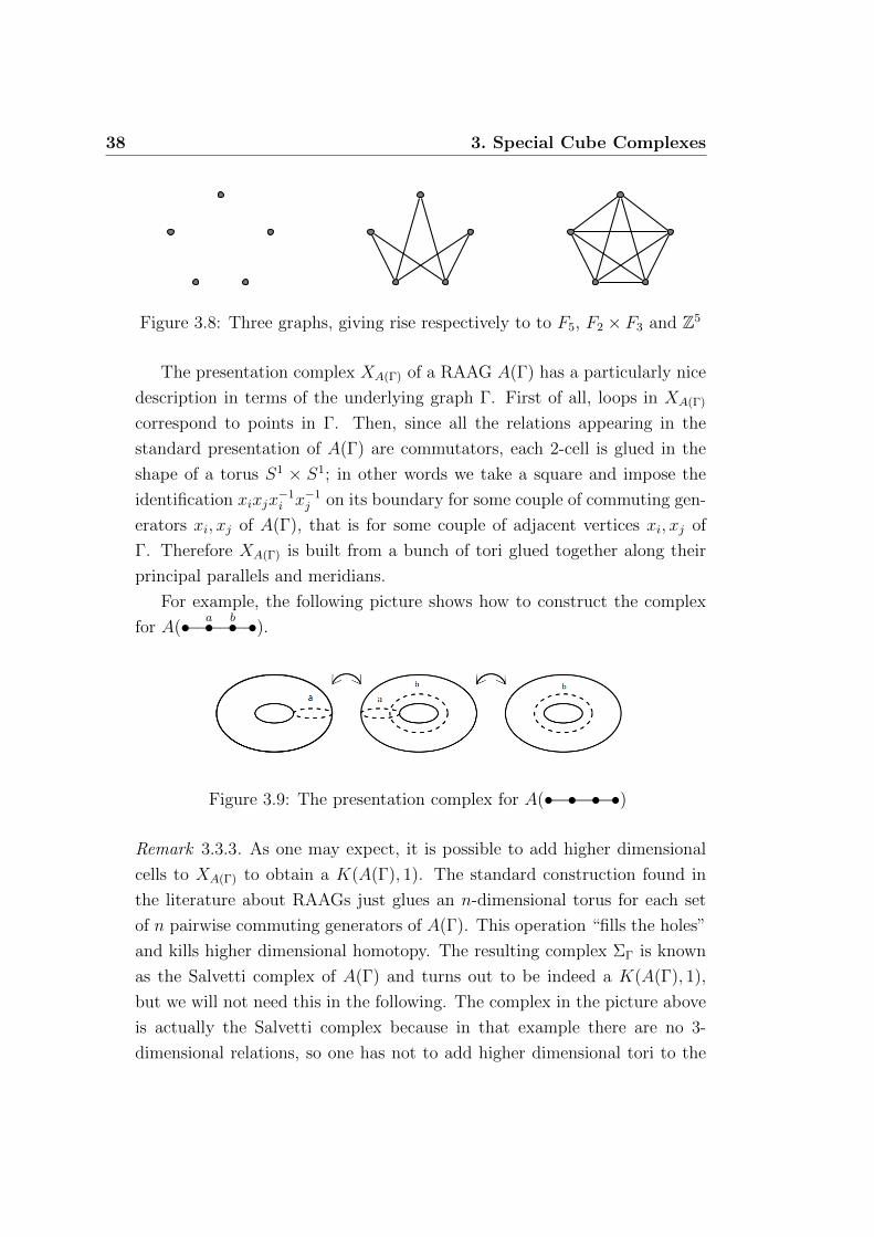
38 3. Special Cube Complexes
Figure 3.8: Three graphs, giving rise respectively to to F5, F2 × F3 and Z5
The presentation complex XA(Γ) of a RAAG A(Γ) has a particularly nice
description in terms of the underlying graph Γ. First of all, loops in XA(Γ)
correspond to points in Γ. Then, since all the relations appearing in the
standard presentation of A(Γ) are commutators, each 2-cell is glued in the
shape of a torus S1 × S1; in other words we take a square and impose the
identification xixjx−1i x−1
j on its boundary for some couple of commuting gen-
erators xi, xj of A(Γ), that is for some couple of adjacent vertices xi, xj of
Γ. Therefore XA(Γ) is built from a bunch of tori glued together along their
principal parallels and meridians.
For example, the following picture shows how to construct the complex
for A(•−−a•−−b•−−•).
Figure 3.9: The presentation complex for A(•−−•−−•−−•)
Remark 3.3.3. As one may expect, it is possible to add higher dimensional
cells to XA(Γ) to obtain a K(A(Γ), 1). The standard construction found in
the literature about RAAGs just glues an n-dimensional torus for each set
of n pairwise commuting generators of A(Γ). This operation “fills the holes”
and kills higher dimensional homotopy. The resulting complex ΣΓ is known
as the Salvetti complex of A(Γ) and turns out to be indeed a K(A(Γ), 1),
but we will not need this in the following. The complex in the picture above
is actually the Salvetti complex because in that example there are no 3-
dimensional relations, so one has not to add higher dimensional tori to the

3.3 Virtual Embedding in RAAGs 39
presentation complex. For further properties of the Salvetti complex also
have a look at 3.4.5 below.
3.3.2 A-typing of a Square Complex
To go from a cube complex to a RAAG we need a simplicial graph. For our
purposes it will be enough to consider square complexes, i.e. 2-dimensional
cube complexes.
Definition 3.3.4. Let B a square complex. We define the hyperplane graph
(or intersection graph) ΓB as follows: take a vertex for each hyperplane of B
and join two vertices if and only if the corresponding hyperplanes intersect.
Remark 3.3.5. We observe that
• By construction ΓB has no bigon.
• If B has no selfintersecting hyperplanes, then ΓB has no loops.
In this case ΓB is a simplicial graph and we can construct A(ΓB). We can
think of this group as presented by
A(ΓB) = 〈xi | [xi, xj] iff xi ∩ xj 6= ∅〉
where the xi denote either the hyperplanes or the walls of B. Let XB :=
XA(ΓB) the presentation complex associated to this presentation of A(ΓB).
We can be even more explicit: loops in XB correspond to hyperplanes (or
walls) in B and there is a 2-cell (glued as a torus as describer before) for each
couple of intersecting hyperplanes (or walls).
Lemma 3.3.6. If hyperplanes in B are embedded and 2-sided then we can
find a combinatorial map τA : B → XB.
Proof. By hypothesis, we can coherently orient each wall of B. So it is
possible to define a map f on the 1-skeleton which sends each edge a of B
to the loop in XB associated to the wall through a in a way that preserves
orientations. But then such a map is easily extended to squares of B in the
following way. Take a square S of B and let Wi,Wj the walls containing
its edges; they are distinct walls since B has embedded hyperplanes. The
40 3. Special Cube Complexes
perimeter of S is mapped by f on the loop xixjx−1i x−1
j where xi, xj are the
loops corresponding to the walls Wi,Wj. Since Wi,Wj intersect in S there
is a square (a torus) in XB with boundary this loop, and it is unique by
construction of ΓB. Then we just send S to this torus.
Definition 3.3.7. If B is a square complex with embedded and 2-sided
hyperplanes, we say that the map τA : B → XB in the previous lemma is
an A-typing of B. In the following, if we talk about A-typings we implicitly
suppose that B is a square complex with embedded and 2-sided hyperplanes
so that everything is well-defined.
Now we want to show that if moreover B is A-special, then any A-typing
is π1-injective. This will follow from a close inspection of elementary homo-
topies in XB and the fact that A-speciality will allow us to pullback such
homotopies.
We recall from 3.2.9 that, by cellular approximation, we can reduce the
study of homotopies of paths in a cube complex to the consideration of ele-
mentary homotopies of an edge-path x1 . . . xn, which can only take one of
these two forms:
1. x1 . . . xi−1xix−1i xi+1 . . . xn ' x1 . . . xi−1xi+1 . . . xn
2. x1 . . . xixj . . . xn ' x1 . . . xhxk . . . xn whenever xixjx−1k x−1
h is the (ori-
ented) perimeter of some square of X
In the case of XB, the homotopy of type 2 takes the particular form
2. x1 . . . xixj . . . xn ' x1 . . . xjxi . . . xn whenever the hyperplanes xi and
xj intersect in B
This is just because squares are glued along commutators of edges if and only
if the corresponding hyperplanes intersect. Here we are using the symbols xi
to denote loops in XB and also the corresponding walls or hyperplanes in B.
Theorem 3.3.8. Let B be an A-special square complex. Then any A-typing
τA : B → XB induces an embedding τA∗ : π1(B) ↪→ π1(XB) = A(ΓB).
3.3 Virtual Embedding in RAAGs 41
Proof. Let γ be an edge-loop in B and let γ∗ = τA(γ) be its image in XB.
First observe that γ and γ∗ have the same combinatorial length. Suppose γ∗
is nullhomotopic in XB. This means that there is a sequence of homotopies
from γ∗ to the unique constant path in the base point of XB. We have to
consider what happens to γ in B when γ∗ undergoes a homotopy in XB.
1. If in XB we see a homotopy of the first type, i.e. xix−1i ' ∅, it means
that γ has two consecutive edges from the same wall, but the second
with opposite orientation. If these two edges were distinct, then they
would realize a configuration of self-intersection (if they lied in some
square) or of direct osculation (if not); but both cases would be absurd
since B is A-special. Thus these two edges are actually the same edge
(traversed with different orientations), then we have that γ has a piece
of the form aa−1 which can be homotoped to a point.
2. If in XB we see a homotopy of the second type, i.e. xixj ' xjxi,
it means that γ has two consecutive edges from two different walls,
but these walls intersect somewhere in B. The case in which they do
not lie in a square is absurd because it would give a configuration of
interosculation in B, which is A-special. So these edges lie in a square,
then their concatenation can be homotoped to the concatenation of the
two opposite edges (preserving orientation).
Therefore we see that every homotopy of γ∗ gives a homotopy of γ of the same
kind. In particular, if γ∗ undergoes a homotopy which reduces its length by
2, then γ undergoes a homotopy which reduces its length by 2 as well1. This
allows us to conclude that if γ∗ is nullhomotopic then γ is nullhomotopic. As
a consequence the A-typing τA is π1-injective.
Remark 3.3.9. We explicitly observe that the square complex XB considered
in the above construction and proof is actually the 2-skeleton of the Salvetti
complex ΣΓBof the RAAG A(ΓB) associated to the hyperplane graph ΓB
of B. The Salvetti complex of a RAAG was introduced in 3.3.3, and more
about it will be said in section 3.4, where it will be showed that it carries an
interesting geometry of non-positive curvature.
1Notice that this proof also shows that nullhomotopic edge-loops have even length.
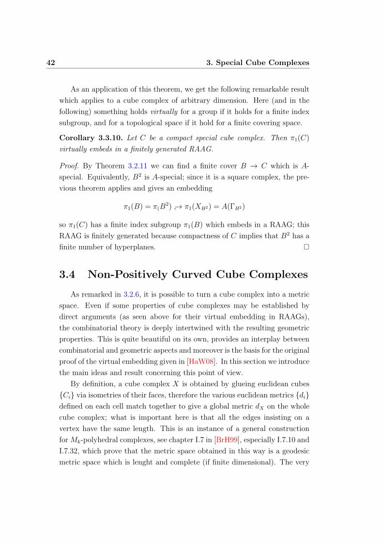
42 3. Special Cube Complexes
As an application of this theorem, we get the following remarkable result
which applies to a cube complex of arbitrary dimension. Here (and in the
following) something holds virtually for a group if it holds for a finite index
subgroup, and for a topological space if it hold for a finite covering space.
Corollary 3.3.10. Let C be a compact special cube complex. Then π1(C)
virtually embeds in a finitely generated RAAG.
Proof. By Theorem 3.2.11 we can find a finite cover B → C which is A-
special. Equivalently, B2 is A-special; since it is a square complex, the pre-
vious theorem applies and gives an embedding
π1(B) = π(B2) ↪→ π1(XB2) = A(ΓB2)
so π1(C) has a finite index subgroup π1(B) which embeds in a RAAG; this
RAAG is finitely generated because compactness of C implies that B2 has a
finite number of hyperplanes.
3.4 Non-Positively Curved Cube Complexes
As remarked in 3.2.6, it is possible to turn a cube complex into a metric
space. Even if some properties of cube complexes may be established by
direct arguments (as seen above for their virtual embedding in RAAGs),
the combinatorial theory is deeply intertwined with the resulting geometric
properties. This is quite beautiful on its own, provides an interplay between
combinatorial and geometric aspects and moreover is the basis for the original
proof of the virtual embedding given in [HaW08]. In this section we introduce
the main ideas and result concerning this point of view.
By definition, a cube complex X is obtained by glueing euclidean cubes
{Ci} via isometries of their faces, therefore the various euclidean metrics {di}defined on each cell match together to give a global metric dX on the whole
cube complex; what is important here is that all the edges insisting on a
vertex have the same length. This is an instance of a general construction
for Mk-polyhedral complexes, see chapter I.7 in [BrH99], especially I.7.10 and
I.7.32, which prove that the metric space obtained in this way is a geodesic
metric space which is lenght and complete (if finite dimensional). The very

3.4 Non-Positively Curved Cube Complexes 43
nice thing about this metric space is that many of its geometric features are
encoded in the underlying combinatorics.
Definition 3.4.1. A flag complex is a simplicial complex in which {k + 1}pairwise adjacent vertices always span a k-simplex.
In other words a flag complex is determined by its 1-skeleton: every time
you see the 1-skeleton of a k-simplex, there actually is a k-simplex, no holes
allowed. Recall from 3.1.9 that a cube complex is called simple when the
link of each vertex is simplicial complex (and that all the cube complex we
consider are simple).
Definition 3.4.2. We say a cube complex X is NPC if the link of each vertex
is a flag complex.
Example 3.4.3. The link of a vertex in I3 is a 2-simplex, which is of course
a flag complex, thus a cube is NPC; on the other hand the link of a vertex
in ∂I3 is the complete graph on 3 vertices, which is not flag. Notice that the
geometric realization of ∂I3 is homeomorphic to a sphere.
The acronym NPC stands for non-positively curved. As one may expect
this is because the metric space (X, dX) defined above is non-positively curved
in the sense of the CAT(k) condition (1.2.4). This is actually the case, as
Gromov pointed out in his seminal paper on hyperbolic groups [Gro87].
Theorem 3.4.4 (Gromov Link Condition). A finite dimensional cube com-
plex has non-positive curvature if and only if it is NPC.
For a self contained discussion of this result see [BrH99], chapter II.5,
where this is Theorem 5.20. Moreover a simply connected NPC cube complex
is also called a CAT(0) cube complex, since it is actually a CAT(0) metric
space.
Remark 3.4.5. In 3.3.3 we introduced the Salvetti complex ΣΓ of a RAAG
A(Γ). It directly follows from its construction that each link is a flag complex,
thus ΣΓ is an NPC cube complex. As a result its universal cover is a CAT(0)
cube complex; it is contractible by 1.2.7, which implies that the Salvetti
complex ΣΓ is a K(A(Γ), 1).
44 3. Special Cube Complexes
The correspondence between combinatorial and geometric properties also
holds for maps: a local isometry in the combinatorial sense of 3.2.5 turns out
to be a local isometry in the metric sense. Moreover one has the following.
Proposition 3.4.6. Any A-typing of an A-special square complex is a local
isometry into the 2-skeleton of the Salvetti complex of the associated hyper-
plane graph.
The idea of the proof of this is essentially the same idea behind our
investigation of elementary homotopies in 3.3.8. This fact, combined with
3.4.5 and 1.2.8 gives another proof of the virtual embedding in a RAAG.
However we remark that a precise proof of this involves some quite technical
steps. For instance one has to show that a special cube complex is NPC,
which in turns needs the fact that a NPC square complex admits a canonical
NPC cube completion such that any map defined on the square complex
extends to the whole completion. These issues are addressed by Haglund
and Wise in the appendix of [HaW08].
Chapter 4
Decompositions of 3-Manifolds
The topology of a surface can be studied cutting it along embedded curves
(1-codimensional submanifolds) and thus producing simpler pieces; in a si-
milar fashion 3-dimensional manifolds can be cut along embedded surfaces
(which are the 1-codimensional objects here).
In this chapter we introduce the study of 3-dimensional manifolds from
the point of view of their decomposition along surfaces. This approach will
provide us with some useful reduction as well as some deep ideas. The con-
tents are organized according to the increasing complexity of the surfaces we
want to cut along.
The 3-manifolds in this chapter are always assumed to be compact, con-
nected and orientable. If S is a surface in M we denote by M\\S the compact
(but possibly disconnected) submanifold of M obtained by removing an open
tubular neighborhood of S. We will also say that S is separating (respect-
ively, non-separating) if M \ \S is disconnected (respectively, connected).
First of all we recall the fundamental theorem of low-dimensional topo-
logy, which will be implicitly used in the following.
Theorem (Moise). Every topological manifold of dimension n ≤ 3 can be
given a differentiable structure and a piecewise linear structure in a unique
way, up to isomorphism in the respective category.
A standard reference for results concerning smoothings and triangulations
of topological manifolds is [KS77].
45

46 4. Decompositions of 3-Manifolds
4.1 Prime Decomposition
The simplest kind of surface one can find in a 3-manifold is the sphere S2,
so we begin with the study of spheres in 3-manifolds. Standard references
for the material in this section are [Hat] and [Hem76]. Both of them date
back before Perelman’s proof of Poincare Conjecture1. In this section we try,
where possible, to give shorter proofs of classic result by exploiting this new
strong tool.
Definition 4.1.1. An embedded sphere S in a 3-manifold M is essential if
it does not bound a ball and if it is not a boundary component. M is said to
be irreducible if it does not contain an essential sphere; in other words every
sphere in M either bounds a ball or is a boundary component.
Remark 4.1.2. If a sphere bounds a ball then it is of course homotopically
trivial, i.e. it can be continuously contracted to a point in M . The celebrated
Sphere Theorem by Papakyriakopoulos (see Theorem 4.3 in [Hem76]) roughly
states that every non trivial class in π2(M) gives rise to an embedded sphere,
giving a strong converse to the previous statement. This means that M is
irreducible if and only if π2(M) = 1, which translates a geometric condition
into a homotopy-theoretic one.
Example 4.1.3. By a classic result of Alexander2, every sphere in R3 bounds
a ball. Therefore R3 is a (non compact) irreducible manifold, which is of
course the local model for any (compact or not) manifold. In other words
every interior point in a 3-manifold sits inside a ball whose boundary is an
inessential sphere. Building on the same result one can prove that S3 is
irreducible as well: every embedded sphere bounds a ball (on both sides).
Example 4.1.4. Consider the manifold S2× I. The spheres S2×{−1} and
S2 × {1} are not essential, simply because they are boundary components.
But the sphere S2 × {0} is essential. If we glue the boundary components
together we get the product S2 × S1 (if we use an orientation reversing
homeomorphism of S1) or the twisted (non trivial) bundle S2×S1 (if we
1The Poincare Conjecture claims that the only closed orientable simply-conncected
3-manifold is S3. Perelman proved this is true in a series of papers on the arXiv in 2002-3.2A detailed proof can be found in Theorem 1.1 of [Hat].
4.1 Prime Decomposition 47
choose an orientation preserving omeomorphism of S1); in both cases the
fiber F of the bundle is an essential sphere. Since we are working with
orientable manifolds, we will forget about the second one.
We are interested in understanding what happens when we cut along a
sphere S (which is not a boundary component) in a 3-manifold M . If the
sphere S is not essential, then it bounds a ball and thus disconnects M .
As a result M \ \S = M ′ t B3, where M ′ is a 3-manifold with (at least)
one spherical boundary component and B3 is a closed 3-ball. This is just the
same as representing M as M#S3, which are exactly the manifolds we obtain
if we cap off the spherical boundaries resulting from the cutting procedure.
Motivated by this simple case, we turn our attention to the operation of
connected sum. To get a first taste of how decomposing in a connected sum
reduces the topological complexity of the manifolds involved, we consider the
following lemma, which is a standard application of Seifert-van Kampen and
the fact that S2 is simply connected.
Lemma 4.1.5. If M = M1#M2 then π1(M) ∼= π1(M1) ∗ π1(M2).
We are now ready for the following definition.
Definition 4.1.6. A 3-manifold is said to be prime if every time it can be
written as a connected sum M = M1#M2 then we have that either M1 = S3
or M2 = S3.
This definition is exactly the same as the previous definition of irreducible,
modulo one of the examples discussed above.
Proposition 4.1.7. M is prime if and only if it is either irreducible or
homeomorphic to S2 × S1.
Proof. Suppose M is prime and let S be an embedded sphere in M . We have
two cases here:
1. If S is separating then let M1 and M2 denote the two components of
M \\S, which have ∂Mi∼= S. Let Mi be the manifold obtained capping
∂Mi with a 3-ball. Then M = M1#M2. Since M is prime we have that
one of the connected summands is just S3; let’s say M1 = S3; but this
implies M1 = B3, so S bounds a ball and M is irreducible.
48 4. Decompositions of 3-Manifolds
2. If S is non-separating, then we can find a curve γ in M intersecting S
in a single point trasversely and a tubular neighborhood R of S ∪ γ.
Then we have that R is homeomorphic to S2×S1 with a ball removed
and that ∂R is a sphere which disconnects M . By the discussion of the
previous case we have that M = (S2× S1)#N for some 3-manifold N .
But since M is prime we have N = S3 and M = S2 × S1.
For the reverse implication, we show that an irreducible manifold is neces-
sarily prime and that the same holds for S2×S1 even if it is not irreducible.
1. Suppose M is irreducible and M = M1#M2. Then M is obtained from
N1 = M1 \B3 and N2 = M2 \B3 by glueing them along the boundary
sphere; this sphere bounds both of them in M and by irreducibility one
of them, say N1, is just a ball, which means that M1 = S3.
2. Now suppose S2 × S1 = U#V . By 4.1.5 we have Z ∼= π(S2 × S1) ∼=π1(U) ∗ π1(V ), and so we get that one of the summands, say U , is
simply connected. From the definition of connected sum, we have a
2-sphere S ⊂ S2 × S1 such that (S2 × S1) \ \S has two components
U ′ and V ′ which are the compact manifolds with boundary a sphere
obtained by removing a 3-ball from U and V respectively. Since S is
simply connected, by Seifert-van Kampen we have that π1(U) = π1(U ′)
(and also π1(V ) = π1(V ′)); in particular U ′ is simply connected. The
universal cover of S2 × S1 is S2 × R ∼= R3 \ {0}, and U ′ lifts to an
homeomorphic copy U ′ of itself here. Since ∂U ′ is a sphere in R3, it
bounds a ball by 4.1.3, so U ′ is a ball and then U ′ is a ball too. This
implies that U ∼= S3 and thus S2 × S1 is prime.
It turns out that connected sum is the right thing to look at when cutting
along embedded spheres, as the following result shows.
Theorem 4.1.8 (Prime Decomposition - Kneser 1929, Milnor 1962). Each
3-manifold M can be decomposed as a connected sum of a finite number of
prime 3-manifolds M = P1# . . .#Pn. This decomposition is unique up to
the order of the factors and up to insertion or deletion of S3’s factors.

4.2 Incompressible Surfaces 49
The classical proof is combinatorial and can be found in [Hat] or [Hem76]:
it is straightforward but quite technical. Here we give a short proof of the
existence of the decomposition in the closed case, which nevertheless relies
on the Poincare Conjecture.
Proof of Theorem 4.1.8. If M has no essential spheres, then it is irreducible
and so prime, by 4.1.7. Otherwise M will contain some essential spheres.
From the proof of 4.1.7 it follows that splitting S along a non-separating
sphere allows to decompose M as a connected sum M = M ′#(S2 × S1) for
a suitable M ′, i.e. we can pull out a prime factor. Then iterating this we are
able to decompose M as M = N#(S2 × S1)# . . .#(S2 × S1), where N is a
3-manifold in which every essential sphere is separating.
Now we keep on splitting N along such separating spheres until we are
able to find them and we obtain M = #i∈IPi, where Pi is prime and closed
(since M was) and I possibly infinite. By 4.1.5 we get π1(M) = ∗i∈Iπ1(Pi).
But since fundamental groups of manifolds are finitely generated, we have
that π1(Pi) = 1 for almost all i ∈ I, and by Poincare Conjecture this means
that Pi ∼= S3 for almost all i ∈ I. The thesis follows since N#S3 = N for
every 3-manifold N .
Since we have seen that a prime factor is either homeomoprhic to S2×S1
or irreducible, this theorem essentially reduces the study of 3-manifolds to
that of irreducible 3-manifolds.
4.2 Incompressible Surfaces
In the previous section we have described the theory of cutting along
spheres, and this has required some “ad hoc” techniques. Since the theory
for higher genus surfaces is more uniform, in this section we gather the main
definitions and results that will be used in the following ones. Throughout
this section M will denote a compact, connected and orientable 3-manifold,
and S a compact orientable surface embedded in M , with no sphere compo-
nents and not necessarily connected.

50 4. Decompositions of 3-Manifolds
Definition 4.2.1. When S is connected, we say that S is 2-sided (respect-
ively 1-sided) if the normal bundle to S is trivial (respectively non trivial).
This definition can be extended to a non connected surface such that all of
its components are 2-sided (or all are 1-sided).
Remark 4.2.2. One may expect that 2-sidedness is equivalent to orientability;
this holds if M is orientable. But in full generality the two properties are not
the same; we can find examples of each of the four possible combinations:
1. S2 ⊂ S2 × S1 is orientable and 2-sided;
2. S1 × S1 ⊂ RP2 × S1 is orientable but 1-sided;
3. RP2 ⊂ RP2 × S1 is non orientable but 2-sided;
4. RP2 ⊂ RP3 is non orientable and 1-sided.
Definition 4.2.3. A surface S ⊂M without disk components is incompress-
ible if it is properly embedded (i.e. embedded so that ∂S = S ∩ ∂M) and if
for every disk D ⊂ M with D ∩ S = ∂D there is another disk D′ ⊂ S such
that ∂D = ∂D′.
Figure 4.1: An incompressible surface
The idea is that if S is incompressible and we cut along ∂D and cap
off the resulting boundaries with disks, we are not actually simplifying its
topology, but we are just splitting off a sphere.
Example 4.2.4. Each surface (different from a union of spheres) in R3 or
S3 is compressible.
The following lemma gives a homotopy-theoretic translation of this geo-
metric definition.

4.2 Incompressible Surfaces 51
Lemma 4.2.5. Let S ⊂ M be a 2-sided surface3. Then S is incompressible
if and only if it is π1-injective, i.e. π1(S) ↪→ π1(M).
Proof. Let S be incompressible and suppose π1(S)→ π1(M) is not 1-1. Let
γ be a loop which is nullhomotopic in M but not in S. Let f : D2 →M the
homotopy (in M) between γ and a point. By Stalling’s Loop Theorem (see
Theorem 4.2 in [Hem76]) we can choose f to be injective, so that γ bounds
a disk in M . Since it is not nullhomotopic in S it does not bound a disk in
S, which is absurd by incompressibility assumption.
Suppose now S is π1-injective and let D ⊂ M a disk with D ∩ S = ∂D.
Then ∂D represents a class in π1(S) ↪→ π1(M), and is trivial in π1(M) since
here it bounds D. But by injectivity it also represents the trivial class in
π1(S). But a nullhomotopic loop on a surface bounds a disk, so we see S is
incompressible.
Example 4.2.6. Here is an example of incompressible surface. This is much
more interesting than the previous one and will concern us also during the
next chapters. Let M be a surface bundle over S1, with fiber some fixed
closed orientable surface4 S of genus g ≥ 1. From the long exact sequence of
homotopy groups associated to this fibration we extract the following piece
0 = π2(S1)→ π1(S)→ π1(M)
from which we get that S is π1-injective and thus incompressible by 4.2.5.
Since the base space of this kind of bundle is just S1, the topological structure
is quite easy to understand. Removing a point from the base is equivalent to
removing a fiber surface from the bundle: this produces a product manifold
S × [0, 1]. This means that M is a mapping torus for some homeomorphism
of S to itself; in other words it can be obtained as
M = S × [0, 1]�(p, 0) ∼ (ϕ(p), 1)
for some ϕ ∈ Homeo(S).
3Since our M is always orientable, by the previous remark this is the same as saying
“let S ⊂M be an orientable surface”.4In Chapter 5, we will say that in this case M fibers over the circle, or just that M is
fibered.

52 4. Decompositions of 3-Manifolds
4.3 JSJ Decomposition
Once we have established the Prime Decomposition we can reduce the
study of (compact oriented) 3-manifolds to the study of their prime factors.
Among these we have some S2×S1’s and the generic factors are irreducible.
So the natural thing to do now is to take irreducible manifolds and try to
cut along embedded tori.
Definition 4.3.1. An irreducible manifold M is atoroidal if every incom-
pressible torus is isotopic to some component of ∂M .
In some intuitive sense, atoroidal manifolds are to incompressible tori
what irreducible manifolds are to essential spheres. The expectation (mo-
tivated from the analogy with the Prime Decomposition) is that we can
cut along incompressible tori until we are left with atoroidal pieces. Notice
anyway that here we are not capping the resulting boundaries as we did
in the Prime Decomposition. This is due to the fact that if you want to
fill a spherical boundary component by glueing a ball, you have to choose
an automorphism of the boundary sphere, and there is essentially only one
choice (up to orientation and isotopy): the mapping class group of the sphere
is trivial. On the other hand the torus has a non trivial mapping class group,
so there is no canonical way of capping the boundaries.
In the Prime Decomposition we do not actually cut until we have only
irreducible pieces: when we meet some exceptional (but nice enough) piece
(i.e. S2×S1) we do not cut it along one of its essential surfaces, but content
ourselves with a decomposition in prime factors. In an analogous way, here
we get some exceptional pieces which are nice enough to deserve not to be
split. These pieces are the so-called Seifert manifolds (see next paragraph).
Theorem 4.3.2 (JSJ Decomposition - Jaco, Shalen, Johanson, 1978). Every
irreducible 3-manifold M admits a finite collection of disjoint incompressible
tori T1, . . . , Tn such that the connected components of M \ \ (T1 ∪ · · · ∪ Tn)
are either atoroidal or Seifert manifolds. A minimal such collection is unique
up to isotopy.
Remark 4.3.3. Before introducing Seifert manifolds, we observe that the ex-
ceptional piece S2 × S1 contains no incompressible torus: since a torus in
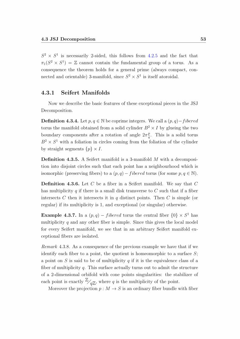
4.3 JSJ Decomposition 53
S2 × S1 is necessarily 2-sided, this follows from 4.2.5 and the fact that
π1(S2 × S1) = Z cannot contain the fundamental group of a torus. As a
consequence the theorem holds for a general prime (always compact, con-
nected and orientable) 3-manifold, since S2 × S1 is itself atoroidal.
4.3.1 Seifert Manifolds
Now we describe the basic features of these exceptional pieces in the JSJ
Decomposition.
Definition 4.3.4. Let p, q ∈ N be coprime integers. We call a (p, q)−fiberedtorus the manifold obtained from a solid cylinder B2 × I by glueing the two
boundary components after a rotation of angle 2π pq. This is a solid torus
B2 × S1 with a foliation in circles coming from the foliation of the cylinder
by straight segments {p} × I.
Definition 4.3.5. A Seifert manifold is a 3-manifold M with a decomposi-
tion into disjoint circles such that each point has a neighbourhood which is
isomorphic (preserving fibers) to a (p, q)− fibered torus (for some p, q ∈ N).
Definition 4.3.6. Let C be a fiber in a Seifert manifold. We say that C
has multiplicity q if there is a small disk transverse to C such that if a fiber
intersects C then it intersects it in q distinct points. Then C is simple (or
regular) if its multiplicity is 1, and exceptional (or singular) otherwise.
Example 4.3.7. In a (p, q) − fibered torus the central fiber {0} × S1 has
multiplicity q and any other fiber is simple. Since this gives the local model
for every Seifert manifold, we see that in an arbitrary Seifert manifold ex-
ceptional fibers are isolated.
Remark 4.3.8. As a consequence of the previous example we have that if we
identify each fiber to a point, the quotient is homeomorphic to a surface S;
a point on S is said to be of multiplicity q if it is the equivalence class of a
fiber of multiplicity q. This surface actually turns out to admit the structure
of a 2-dimensional orbifold with cone points singularities: the stabilizer of
each point is exactly Z�qZ, where q is the multiplicity of the point.
Moreover the projection p : M → S is an ordinary fiber bundle with fiber

54 4. Decompositions of 3-Manifolds
S1 in the complement of the exceptional points. If one likes the orbifold
machinery, it makes sense to call p an orbifold bundle.
The reason why we are dealing with this point of view is that Seifert
manifold have been explicitly classified in terms of (invariants of) the base
orbifold and the bundle projection. Lens spaces and S1-bundles over ori-
entable compact surfaces belong to this classification.
4.4 Geometric Decomposition
The previous decompositions deal with homotopy-theoretic properties of
the manifold: once you perform a Prime Decomposition on your manifold,
every sphere you find will be not essential, and the same can be said about
tori in a JSJ Decomposition (up to some exceptions in both cases, as we
have seen). In this section we want to focus on a decomposition which has a
strong geometric flavour; the decomposition process is quite close to the JSJ
one, but somehow different, as we will see in the end.
It is a classic and well known result that every closed connected orientable
surface admits a geometry (elliptic, euclidean or hyperbolic) according to its
topology (genus 0, 1 or > 1). In [Thu82] Thurston conjectured that the pic-
ture was similar (but different in some crucial features) for the 3-dimensional
world. The main difference with respect to the case of surfaces is first of all
that one cannot expect an arbitrary 3-manifold to admit any “nice geome-
try”, and then that one has to redefine what a “nice geometry” is, because
there are 3-dimensional geometries which are not equivalent to geometries of
constant curvature.
The intuitions of Thurston have guided the research in the field of 3-
dimensional topology for some decades. Only recently (2002-3) Perelman
has provided a proof of Thurston’s Conjecture. The aim of this section is to
give a description of this result and of the concepts involved.
Theorem 4.4.1 (Thurston Geometrisation Conjecture, 1982 - now Perelman
Theorem, 2003). An irreducible 3-manifold M admits a finite collection of
disjoint incompressible tori T1, . . . , Tn such that the interior of each connected
component of M \\ (T1 ∪ · · · ∪ Tn) can be endowed with a geometric structure
4.4 Geometric Decomposition 55
of finite volume.
In the next paragraphs we clarify this statement and give a lot of exam-
ples.
4.4.1 Geometric Structures on Manifolds
Here we want to define a geometry on a manifold; this is essentially done
specifying which are the allowed transformation. In order to give a precise
meaning to the term “geometric structure”, we will need some technical
definitions.
Definition 4.4.2. Let X be a topological space. A pseudogroup G on X is
a collection of local homeomorphisms between open sets of X such that
• the domain of the elements of G covers X,
• G is closed under restriction, composition and inversion, when these
operations are defined,
• being in G is a local property, i.e. if U = ∪Ui and f : U → V is some
local homeomorphism such that f |Ui∈ G then f ∈ G.
Example 4.4.3. Obvious examples are given by the pseudogroups Ck of Ck
local diffeomorphisms between open sets in Rn for k = 0, . . . ,∞ and the pseu-
dogroup H of holomorphic maps between open sets in Cn. Another example
is given by the pseudogroup PL of local piecewise-linear homeomoprhisms
between open sets in Rn.
Example 4.4.4. More generally, if G is a Lie group acting on some manifold
X, it gives rise to a pseudogroup, still denoted G, on X generated by the
restrictions of elements of G to open sets in X. The most interesting example
is given by the isometry group of a Riemannian manifold.
Following the classical definition of a differentiable manifold, we give the
following one.
Definition 4.4.5. Let X be a manifold, G be a pseudogroup on X and M
a topological space.

56 4. Decompositions of 3-Manifolds
• A (G, X)-chart on M is an open set U of M together with a homeomor-
phism ϕU : U → ϕU(U) ⊂ X. Two (G, X)-charts (U,ϕU) and (V, ϕV )
are compatible if the transition map ϕUϕ−1V : ϕV (U ∩V )→ ϕU(U ∩V )
belongs to G.
• M is a (G, X)-manifold if it is Hausdorff, second countable and endowed
with a maximal collection of compatible charts; we also say that M has
a geometric structure of type (G, X).
Example 4.4.6. A Ck-manifold is just a (Ck,Rn)-manifold, a complex mani-
fold is just a (H,Cn)-manifold and a PL-manifold is just a (PL,Rn)-manifold.
This approach allows to treat on a common ground a great variety of
geometries that one can put on manifolds. The idea is that we start with some
model geometry embodied by some manifold X and select some admissible
transformation which belong to that geometry (the pseudogroup) and use
these to construct new manifolds glueing together pieces of X through these
geometry-preserving transformations.
Definition 4.4.7. A pair (G,X) is called a model geometry if
1. X is a connected and simply connected differentiable manifold;
2. G is a Lie group of diffeomorphisms of X acting transitively with com-
pact stabilizers, and is maximal with respect to this property;
3. there exists at least one compact (G,X)-manifold.
Proposition 4.4.8. Every model geometry (G,X) can actually be endowed
with a G-invariant Riemannian metric; therefore G can actually be thought
of as a group of Riemannian isometries.
Proof. Let x ∈ X and choose some inner product (., .) on TxX. Since sta-
bilizers are compact, we can average with respect to Haar measure on the
stabilizer in x and define
< u, v >=
∫Gx
(dgxu, dgxv)dg
This turns out to be a G-invariant inner product on TxX and we get a
Riemannian metric by translating it with the action of G, which is transitive
by hypothesis.
4.4 Geometric Decomposition 57
4.4.2 Thurston’s Eight Geometries
Thurston has classified all the model geometries that can occur in di-
mension 2 and 3. As one may expect, in dimension 2 we find only S2, E2
and H2 with their groups of isometries. Of course also in dimension 3 we
have S3, E3 and H3 with their groups of isometries: these are the so-called
homogeneous geometries and have stabilizers isomorphic to O(3). Compact
representative are respectively given by S3, the 3-torus S1 × S1 × S1 and
the manifold obtained from S3 removing an open tubular neighbourhood of
a trefoil or figure-eight knot.
But, has hinted above, the third dimension leaves enough room for the ex-
istence of non homogeneous model geometries, which have typically smaller
stabilizers. We now give a brief description of some geometries of this kind.
Example 4.4.9. The manifold S2 × R can be endowed with the product
metric; the isometry group of this structure is Isom(S2) × R ∼= O(3) × Rwith stabilizers isomorphic to O(2). A compact manifold with this kind of
geometry is given by S2 × S1.
Example 4.4.10. The same construction can be carried on for H2 × R:
we get an isometry group isomorphic to PSL2R × R with stabilizers again
isomorphic to O(2). Any product S × S1 where S is a hyperbolic surface is
a compact example of this geometry.
Of course the same construction with E2 gives the geometry E3. There
are three more model geometries, which are quite more exotic.
Example 4.4.11. Let SL2R be the universal cover of SL2R. It is possible
to induce a metric on this Lie group from the metric of the hyperbolic plane
H2. The bundle of unit tangent vectors on a closed hyperbolic surface is a
compact representative of this geometry.
Example 4.4.12. Let Nil be the Heisenberg group of upper triangular mat-
rices with real coefficients and unit diagonal. This Lie group is diffeomorphic
to R3. We impose the euclidean inner product at the identity and then
propagate via group multiplication. This gives an invariant metric on Nil.
A compact example is obtained by Nil itself quotienting out the lattice of

58 4. Decompositions of 3-Manifolds
matrices with integer coefficients. Manifolds with this geometry are called
nilmanifolds.
Example 4.4.13. Consider R3 with the group structure given by
(x1, y1, z1) ∗ (x2, y2, z2) := (x1 + exp−z1 x2, y1 + expz1 y2, z1 + z2)
As above we construct a left-invariant metric on this Lie group, and we call
Sol the resulting model geometry and solvmanifold the manifolds modelled
on it. A compact example can be built as follows: let ϕ : R2 → R2 the linear
mapping defined by
A =
(2 1
1 1
)Since it fixes the integer lattice, it descends to a diffeomorphism (of Anosov
type) of the torus T = S1 × S1. The mapping torus of this diffeomorphism
is an example of solvmanifold.
As announced, we have the following theorem of Thurston.
Theorem 4.4.14 (Thurston). A 3-dimensional model geometry (G,X) is
one of the eight geometries discussed above.
Proof. (Sketch, see Theorem 3.15 of [Wil02] for a detailed proof) Since the
metric constructed in 4.4.8 is G-invariant, the stabilizer of a point is a (max-
imal connected) subgroup of O(3), so it must be SO(3), SO(2) or the trivial
group. Now the proof boils down to the inspection of these cases. The first
case is that of homogeneous geometry of constant curvature (S3, E3 and H3).
The second case has 2-dimensional stabilizer and the third dimension is left
free, allowing for “foliated” geometries: here we find S2×R, H2×R, Nil and
SL2R. In the case of trivial stabilizer X is actually a Lie group and from the
classification of 3-dimensional Lie algebras it follows that the only geometry
of this kind is Sol.
Remark 4.4.15. Since S3 is the only closed model geometry, it follows from
the Geometrization Theorem that a closed simply connected 3-manifold is
homeomorphic to S3, which is the statement of Poincare Conjecture.

4.4 Geometric Decomposition 59
4.4.3 A comparison between JSJ and Geometric De-
composition
The interest of Thurston in the Geometrization program stems from the
need of a better understanding of the generic (i.e. atoroidal) pieces arising
from a JSJ Decomposition, the other pieces (i.e. Seifert) being well under-
stood and classified as said before. What Perelman actually proved is the
following:
Theorem 4.4.16 (Perelman). Let M be an irreducible atoroidal manifold.
Then
• (Elliptization Conjecture) if π1(M) is finite then M is elliptic;
• (Hyperbolization Conjecture) if π1(M) is infinite then M is hyperbolic.
It can be proved that an elliptic geometry gives rise to a Seifert structure
(see Theorem 2.8 in [Bon02]). As a consequence we see that “being Seifert”
and “being atoroidal” are not mutually exclusive properties. On the other
hand, from a detailed analysis of the classification of Seifert manifolds, one
can deduce that hyperbolic manifolds are not Seifert. This is what actually
we can obtain:
Theorem 4.4.17. The class of Seifert manifolds coincides with the class of
manifolds which admit a geometry modelled on one of these: S3, E3, S2×R,
H2 × R, SL2R and Nil. Moreover the geometry type is uniquely determined
by the topology of the manifold.
We can therefore state this form of Torus Decomposition Theorem.
Theorem 4.4.18. Every irreducible 3-manifold M admits a finite collection
of disjoint incompressible tori T1, . . . , Tn such that the connected components
of M \ \ (T1 ∪ · · · ∪ Tn) are either hyperbolic or Seifert. A minimal such
collection is unique up to isotopy.
The advantage of this formulation is that the resulting pieces are divided
into two disjoint classes. The study of 3-manifolds is thus reduced to that of
their hyperbolic components.
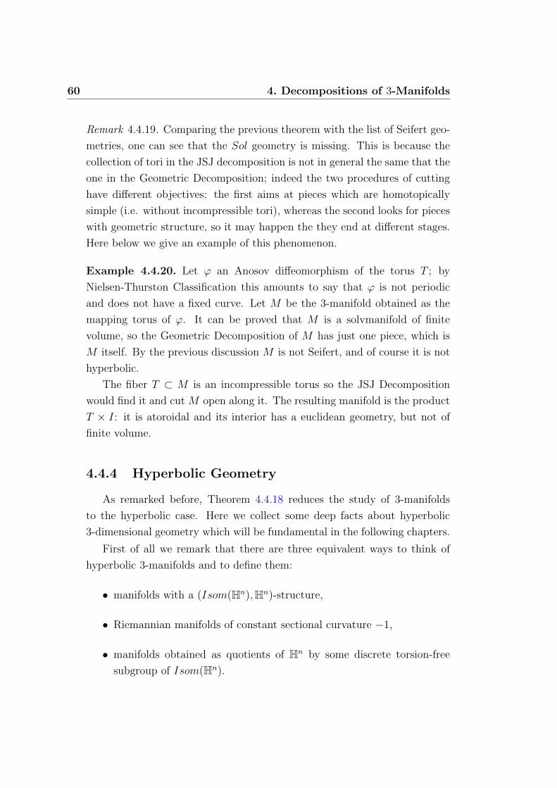
60 4. Decompositions of 3-Manifolds
Remark 4.4.19. Comparing the previous theorem with the list of Seifert geo-
metries, one can see that the Sol geometry is missing. This is because the
collection of tori in the JSJ decomposition is not in general the same that the
one in the Geometric Decomposition; indeed the two procedures of cutting
have different objectives: the first aims at pieces which are homotopically
simple (i.e. without incompressible tori), whereas the second looks for pieces
with geometric structure, so it may happen the they end at different stages.
Here below we give an example of this phenomenon.
Example 4.4.20. Let ϕ an Anosov diffeomorphism of the torus T ; by
Nielsen-Thurston Classification this amounts to say that ϕ is not periodic
and does not have a fixed curve. Let M be the 3-manifold obtained as the
mapping torus of ϕ. It can be proved that M is a solvmanifold of finite
volume, so the Geometric Decomposition of M has just one piece, which is
M itself. By the previous discussion M is not Seifert, and of course it is not
hyperbolic.
The fiber T ⊂ M is an incompressible torus so the JSJ Decomposition
would find it and cut M open along it. The resulting manifold is the product
T × I: it is atoroidal and its interior has a euclidean geometry, but not of
finite volume.
4.4.4 Hyperbolic Geometry
As remarked before, Theorem 4.4.18 reduces the study of 3-manifolds
to the hyperbolic case. Here we collect some deep facts about hyperbolic
3-dimensional geometry which will be fundamental in the following chapters.
First of all we remark that there are three equivalent ways to think of
hyperbolic 3-manifolds and to define them:
• manifolds with a (Isom(Hn),Hn)-structure,
• Riemannian manifolds of constant sectional curvature −1,
• manifolds obtained as quotients of Hn by some discrete torsion-free
subgroup of Isom(Hn).
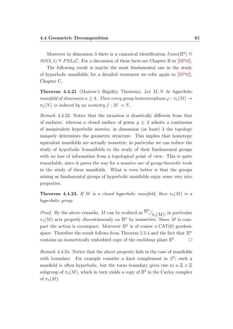
4.4 Geometric Decomposition 61
Moreover in dimension 3 there is a canonical identification Isom(H3) ∼=SO(3, 1) ∼= PSL2C. For a discussion of these facts see Chapter B in [BP92].
The following result is maybe the most fundamental one in the study
of hyperbolic manifolds; for a detailed treatment we refer again to [BP92],
Chapter C.
Theorem 4.4.21 (Mostow’s Rigidity Theorem). Let M,N be hyperbolic
manifold of dimension n ≥ 3. Then every group homomorphism ϕ : π1(M)→π1(N) is induced by an isometry f : M → N .
Remark 4.4.22. Notice that the situation is drastically different from that
of surfaces: whereas a closed surface of genus g ≥ 2 admits a continuum
of inequivalent hyperbolic metrics, in dimension (at least) 3 the topology
uniquely determines the geometric structure. This implies that homotopy
equivalent manifolds are actually isometric; in particular we can reduce the
study of hyperbolic 3-manifolds to the study of their fundamental groups
with no loss of information from a topological point of view. This is quite
remarkable, since it paves the way for a massive use of group-theoretic tools
in the study of these manifolds. What is even better is that the groups
arising as fundamental groups of hyperbolic manifolds enjoy some very nice
properties.
Theorem 4.4.23. If M is a closed hyperbolic manifold, then π1(M) is a
hyperbolic group.
Proof. By the above remarks, M can be realized as Hn�π1(M); in particular
π1(M) acts properly discontinuously on Hn by isometries. Since M is com-
pact the action is cocompact. Moreover Hn is of course a CAT(0) geodesic
space. Therefore the result follows from Theorem 2.3.4 and the fact that Hn
contains no isometrically embedded copy of the euclidean plane E2.
Remark 4.4.24. Notice that the above property fails in the case of manifolds
with boundary. For example consider a knot complement in S3; such a
manifold is often hyperbolic, but the torus boundary gives rise to a Z × Zsubgroup of π1(M), which in turn yields a copy of E2 in the Cayley complex
of π1(M).

62 4. Decompositions of 3-Manifolds
4.5 Haken Manifolds
In this section we get back to the point of view of cutting along embedded
incompressible surfaces and give a general description of the situation for
genus g > 1 surfaces.
Definition 4.5.1. A Haken manifold is a 3-manifold which is irreducible and
contains an incompressible surface.
Remark 4.5.2. The study of these manifolds has a lot to do with the geometric
aspects discussed above, since for a long time they have been the starting
point for any classic (i.e. pre-Perelman) approach to the Geometrization
Conjecture. The reason behind this is that Thurston himself was able to
prove a form of hyperbolization for irreducible atoroidal Haken manifolds M
with χ(∂M) = 0 at the beginning of the 1980’s, well before Perelman’s proof
through parabolic equations. Therefore topologists hoped that some kind of
reduction to the Haken case could lead to a proof of Geometrization.
An algebraic criterion to check whether a manifold is Haken is the fol-
lowing result; here and in the following H∗ denotes singular homology with
integer coefficients.
Lemma 4.5.3. If H1(M) is infinite then M contains an incompressible sur-
face.
Proof. From the classification of finitely generated abelian groups we know
H1(M) ∼= Zn ⊕ T for some integer n and some torsion group T ; by the
hypothesis we have n ≥ 1, therefore we have an epimorphism H1(M) � Z,
which we may precompose with the Hurewicz map to get an epimorphism
ϕ : π1(M) � Z. Since S1 may be taken as a K(Z, 1), from 2.1.16 we get
a map (unique up to basepoint-preserving homotopies) f : M → S1 which
induces ϕ on fundamental groups; in particular since ϕ is non trivial f must
be surjective. For any point p ∈ S1 Lemma 6.5 in [Hem76] implies that f
may be homotoped so that each component of f−1(p) is an incompressible
surface.
With some basic algebraic topology one can convert the previous result
into an easier and more geometric criterion.

4.5 Haken Manifolds 63
Lemma 4.5.4. If ∂M 6= ∅ does not contain only spheres, then H1(M) is
infinite.
Proof. First of all let M the 3-manifold obtained from M capping off all
the boundary spheres with 3-balls. By Seifert-van Kampen and the simply-
connectedness of S2 we compute π1(M) = π1(M) and thus H1(M) = H1(M).
Therefore we may reduce to the case ∂M contains no spheres.
Since ∂M 6= ∅ we can take two copies of M and glue them along their
boundary, getting a closed manifold M ′, which is called the double of M .
Choosing some triangulation it is easy to see that χ(M ′) = χ(M) + χ(M)−χ(∂M) since the two copies of M inside M ′ intersect in ∂M . Now, since M ′
is closed and odd-dimensional, we have by Poincare Duality and Universal
Coefficients Theorem5 that χ(M ′) = 0. So we get χ(M) =χ(∂M)
2≤ 0, since
we have reduced to the case ∂M contains no spheres.
Now, if bi are the Betti numbers of M we have that b0 = 1 since M is
connected and b3 = 0 since ∂M 6= ∅; from the previous discussion we get
1 − b1 + b2 ≤ 0 and so b1 ≥ 1 + b2 ≥ 1, which implies that H1(M) is an
infinite group.
Example 4.5.5. Combining the previous lemmas, we can conclude that any
(compact, connected and orientable) manifold with sufficiently complicated
boundary contains an incompressible surface. For example knot (or link)
complements in S3 contain an incompressible surface, since they have at
least one torus boundary component. Another example of Haken manifold
is given by surface bundles: see Example 4.2.6.
In complete analogy to the case of essential spheres and incompressible
tori, if we have a Haken manifold we can try to cut it open along some
incompressible surface. Let M be a 3-manifold and S ⊂M an incompressible
surface and let M ′ be the (possibly disconnected) manifold M \ \S. We say
M ′ is obtained from M by decomposition along S and also write MS→ M ′.
By construction M ′ can be naturally identified with a closed submanifold of
M . To check that everything goes through as expected we need one more
lemma.
5See [Hat02], Prop. 2.45 for details.

64 4. Decompositions of 3-Manifolds
Lemma 4.5.6. In the above notation M ′ is reducible if and only if M is.
Proof. Suppose M ′ is reducible; then let T be an essential sphere in M ′ ⊂M
that does not bound a ball in M ′. If T bounds a ball in M (but not in
M ′) then S must lie inside this ball. But by 4.2.4 any surface in a ball is
incompressible, but S is not, so T does not bound a ball in M , which means
M is reducible as well.
On the other hand let M be reducible. Choose an essential sphere T ⊂M
which does not bound a ball in M and that minimizes the number k of
components of S ∩ T . If k = 0 then T actually lies in M ′, which is thus
reducible. Otherwise consider an outermost disk D cut by S on T . By
incompressibility of S we can find another disk E ⊂ S such that ∂E = ∂D;
if D ∪ E bounds a ball in M ′ we can isotope D through E; this operation
reduces k, which is absurd by minimality assumption. Otherwise E ∪ Dis an essential sphere in M ′ which does not bound a ball in M ′ and M ′ is
reducible.
Remark 4.5.7. From 4.2.6, 4.5.6 and the fact that product manifolds S × I(with S a closed surface) are irreducible, we get another way to see that
surface bundles over the circle are Haken manifolds.
Corollary 4.5.8. Let M be a Haken manifold. Then any (component of the)
manifold obtained by decomposition along an incompressible surface is again
Haken.
Proof. Let S ⊂ M be an incompressible surface and MS→ M ′. By 4.5.6
M ′ is still irreducible. Moreover M ′ has at least one boundary component
which is not a sphere, i.e. that arising from S (which is not a sphere by the
given definition of incompressible surface). Then it follows from 4.5.4 and
4.5.3 that M ′ contains an incompressible surface and is therefore a Haken
manifold.
As a consequence of the previous result, we can keep on splitting the
result of the first decomposition and get a (a priori infinite) chain of Haken
manifold which get simpler and simpler.

4.5 Haken Manifolds 65
Definition 4.5.9. A series of decomposition M = M0S1→ M1
S2→ . . . of a
Haken manifold along surfaces which are incompressible at each step is called
a hierarchy for M provided it terminates after a finite number of steps.
Remark 4.5.10. The nice thing about Haken manifolds is that it is possible
to prove that a Haken manifold always has a hierarchy. In the case ∂M 6= ∅the above results have to be sharpened a bit to guarantee the surfaces we
split along behave nicely with respect to the boundary. By 4.5.4 and 4.5.3
the final step of any hierarchy for M will always be a 3-manifold with only
spherical boundary component. This implies that a hierarchy for a Haken
manifold can be thought as a procedure to reduce the manifold to a collection
of closed 3-balls.
Remark 4.5.11. Haken manifold owe to the previous remark a lot of nice
features, which we mention just for the sake of completeness; for example:
• we have an algorithm to check whether a given manifold is Haken;
• we have an algorithm to tell if two Haken manifolds are homeomorphic;
• closed Haken manifold are homotopically rigid: they are determined
up to homeomorphism by their fundamental group.
The bad thing about this is that there are non Haken manifolds. So, differ-
ently from the previous approaches, not every 3-manifold can be analysed
via this kind of decomposition. At least a priori.

66 4. Decompositions of 3-Manifolds

Chapter 5
Virtual Fibration of Hyperbolic
3-manifolds
In the last few years the joint work of many mathematicians has shown
that the conclusion of the previous chapter is more pessimistic than it should
be: 3-manifolds are actually much nicer than expected. In 1968 Waldhausen
implicitly proposed the following conjecture.
Conjecture 5.1 (Virtually Haken Conjecture). A compact, orientable, irre-
ducible 3-manifold with infinite fundamental group is virtually Haken, i.e. it
has a finite covering space that is a Haken manifold.
As we have seen in 4.4.3, Geometrization implies that an irreducible
atoroidal manifold has infinite fundamental group if and only if it is hy-
perbolic, therefore we may restrict to the hyperbolic case. Moreover, 4.5.4
let us reduce to the case of closed manifolds.
Conjecture 5.2 (Virtually Haken Conjecture - Thurston’s Hyperbolic state-
ment). A closed hyperbolic 3-manifold is virtually Haken.
This is exactly what Thurston posed as question 16 in his notorious article
[Thu82]. In the same article he posed another problem; before stating it we
introduce the main definition of this chapter.
Definition 5.0.12. A 3-manifold M is said to fiber over the circle if it is a
bundle over S1 with fiber some fixed surface. In the following we also just
67
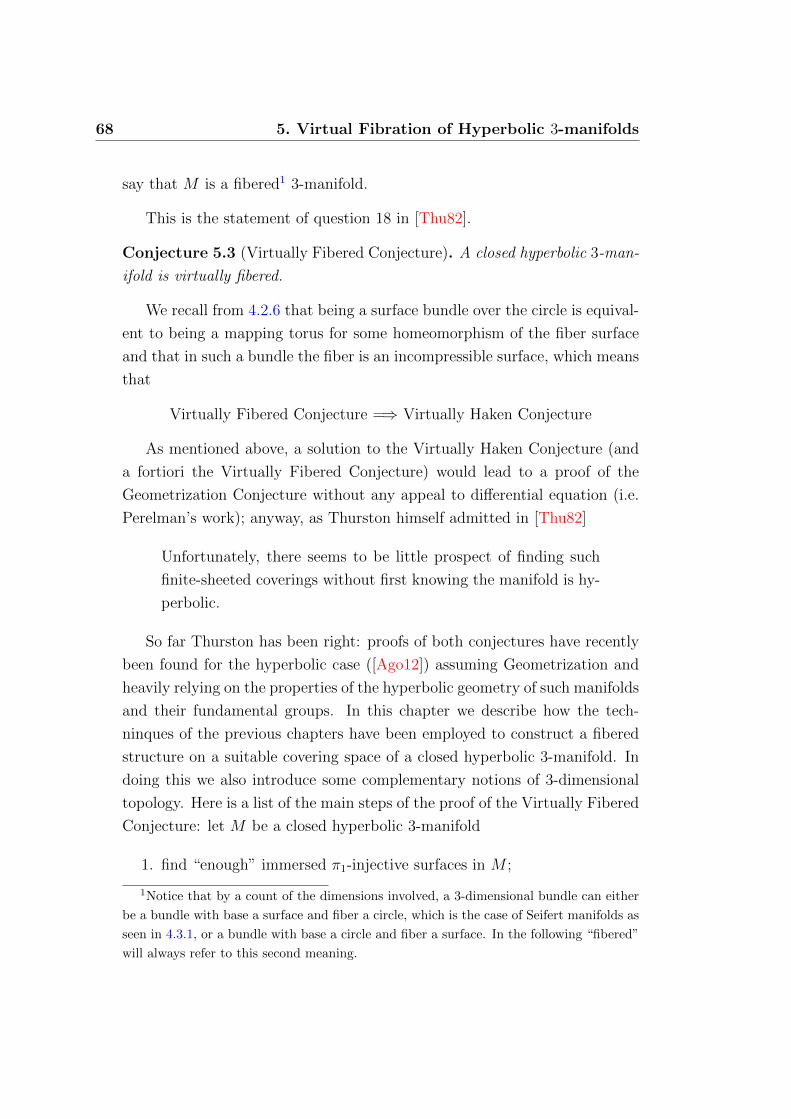
68 5. Virtual Fibration of Hyperbolic 3-manifolds
say that M is a fibered1 3-manifold.
This is the statement of question 18 in [Thu82].
Conjecture 5.3 (Virtually Fibered Conjecture). A closed hyperbolic 3-man-
ifold is virtually fibered.
We recall from 4.2.6 that being a surface bundle over the circle is equival-
ent to being a mapping torus for some homeomorphism of the fiber surface
and that in such a bundle the fiber is an incompressible surface, which means
that
Virtually Fibered Conjecture =⇒ Virtually Haken Conjecture
As mentioned above, a solution to the Virtually Haken Conjecture (and
a fortiori the Virtually Fibered Conjecture) would lead to a proof of the
Geometrization Conjecture without any appeal to differential equation (i.e.
Perelman’s work); anyway, as Thurston himself admitted in [Thu82]
Unfortunately, there seems to be little prospect of finding such
finite-sheeted coverings without first knowing the manifold is hy-
perbolic.
So far Thurston has been right: proofs of both conjectures have recently
been found for the hyperbolic case ([Ago12]) assuming Geometrization and
heavily relying on the properties of the hyperbolic geometry of such manifolds
and their fundamental groups. In this chapter we describe how the tech-
ninques of the previous chapters have been employed to construct a fibered
structure on a suitable covering space of a closed hyperbolic 3-manifold. In
doing this we also introduce some complementary notions of 3-dimensional
topology. Here is a list of the main steps of the proof of the Virtually Fibered
Conjecture: let M be a closed hyperbolic 3-manifold
1. find “enough” immersed π1-injective surfaces in M ;
1Notice that by a count of the dimensions involved, a 3-dimensional bundle can either
be a bundle with base a surface and fiber a circle, which is the case of Seifert manifolds as
seen in 4.3.1, or a bundle with base a circle and fiber a surface. In the following “fibered”
will always refer to this second meaning.

5.1 Cubulation of Groups and Manifolds 69
2. the subgroups they induce in π1(M) allow to construct a cube complex
X with π1(X) = π1(M);
3. since π1(M) is a hyperbolic group, this cube complex turns out to be
compact and (virtually) special;
4. as a result, π1(M) virtually embeds in some RAAG;
5. RAAGs satisfy a certain technical algebraic condition (the RFRS con-
dition);
6. a 3-manifold with RFRS fundamental group admits a fibered cover.
5.1 Cubulation of Groups and Manifolds
By “cubulation of groups” we mean a combinatorial construction which
was first introduced by Sageev in [Sag95] and then in [Sag97]; this construc-
tion takes a group G with a suitable family of subgroups and produces a cube
complex with a G-action. Bergeron and Wise in [BW10] then exploit this
construction to “cubulate” a closed hyperbolic 3-manifold (i.e. to cubulate
its fundamental group), heavily relying on the work [KM09] of Kahn and
Markovic on the existence of almost geodesic surfaces in such a manifold.
5.1.1 Codimension-1 Subgroups
In this paragraph we describe the fundamental ideas behind the cubula-
tion of groups.
Definition 5.1.1. Let G be a finitely generated group and H a subgroup.
In 2.3.6 we have defined the space of ends of G as the space of ends of its
Cayley graph with respect to some generating set. We now define the ends of
G relative to H, denoted Ends(G,H), to be the space of ends of the metric
space obtained as the quotient of the Cayley graph of G modulo the action
of H. We denote by e(G,H) the cardinality of Ends(G,H).
We remark that this definition is well posed since the space of ends is a
quasi-isometric invariant of proper geodesic spaces.
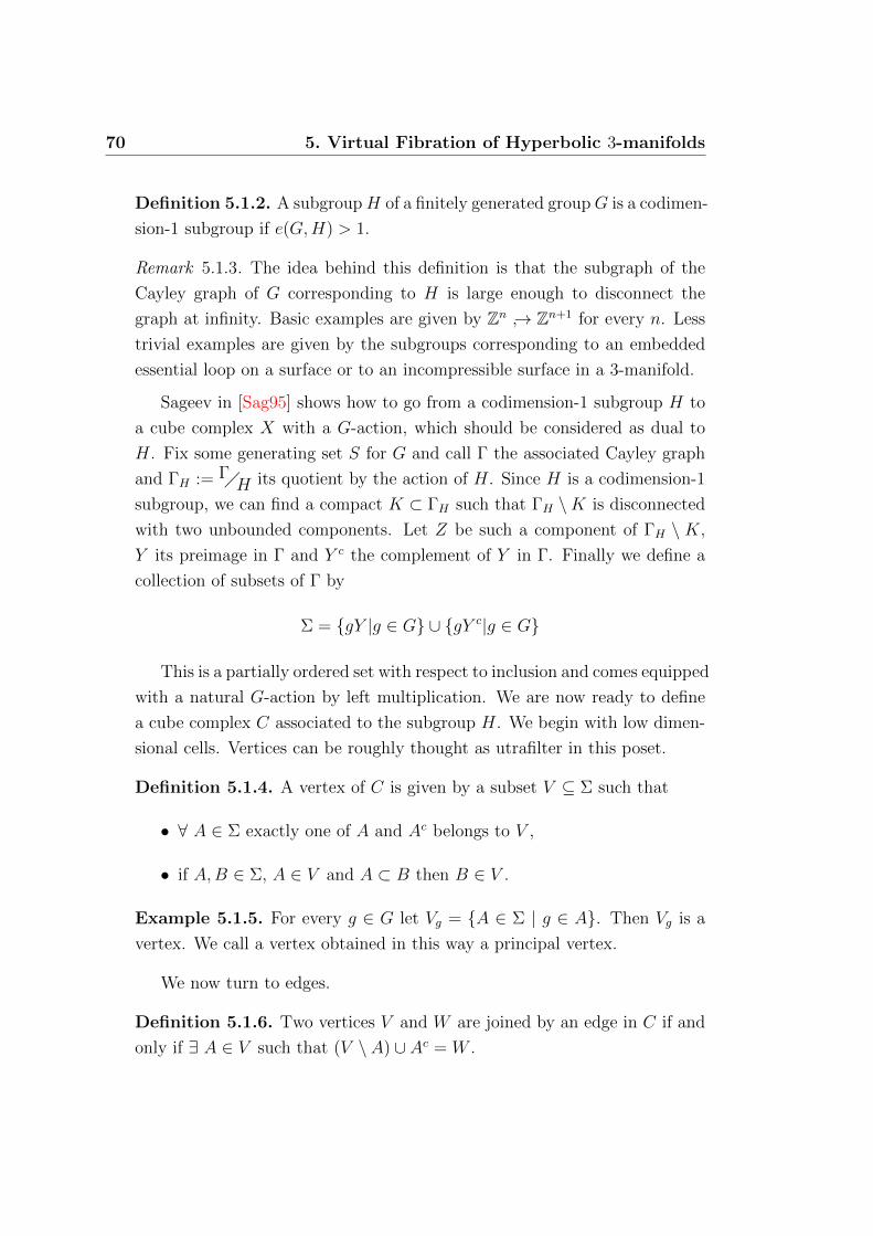
70 5. Virtual Fibration of Hyperbolic 3-manifolds
Definition 5.1.2. A subgroupH of a finitely generated groupG is a codimen-
sion-1 subgroup if e(G,H) > 1.
Remark 5.1.3. The idea behind this definition is that the subgraph of the
Cayley graph of G corresponding to H is large enough to disconnect the
graph at infinity. Basic examples are given by Zn ↪→ Zn+1 for every n. Less
trivial examples are given by the subgroups corresponding to an embedded
essential loop on a surface or to an incompressible surface in a 3-manifold.
Sageev in [Sag95] shows how to go from a codimension-1 subgroup H to
a cube complex X with a G-action, which should be considered as dual to
H. Fix some generating set S for G and call Γ the associated Cayley graph
and ΓH := Γ�H its quotient by the action of H. Since H is a codimension-1
subgroup, we can find a compact K ⊂ ΓH such that ΓH \K is disconnected
with two unbounded components. Let Z be such a component of ΓH \ K,
Y its preimage in Γ and Y c the complement of Y in Γ. Finally we define a
collection of subsets of Γ by
Σ = {gY |g ∈ G} ∪ {gY c|g ∈ G}
This is a partially ordered set with respect to inclusion and comes equipped
with a natural G-action by left multiplication. We are now ready to define
a cube complex C associated to the subgroup H. We begin with low dimen-
sional cells. Vertices can be roughly thought as utrafilter in this poset.
Definition 5.1.4. A vertex of C is given by a subset V ⊆ Σ such that
• ∀ A ∈ Σ exactly one of A and Ac belongs to V ,
• if A,B ∈ Σ, A ∈ V and A ⊂ B then B ∈ V .
Example 5.1.5. For every g ∈ G let Vg = {A ∈ Σ | g ∈ A}. Then Vg is a
vertex. We call a vertex obtained in this way a principal vertex.
We now turn to edges.
Definition 5.1.6. Two vertices V and W are joined by an edge in C if and
only if ∃ A ∈ V such that (V \ A) ∪ Ac = W .

5.1 Cubulation of Groups and Manifolds 71
Remark 5.1.7. Sageev gives some equivalent formulations for this. For ex-
ample, we have that (V \A)∪Ac = W if and only if |V \W | = |W \ V | = 1;
moreover (V \A)∪Ac is a vertex if and only if A is minimal in V with respect
to the induced order.
This defines a graph C.
Definition 5.1.8. We now define X1 to be the subgraph given by the union
of the components of C which contain some principal vertex Vg.
This restriction is needed to forget some undesired vertices. Anyway the
selected subgraph turns out to be still connected.
Example 5.1.9. Let G = Z, H = {0} and Γ =Cay(Z, {1}). Since the
action of H on Γ is trivial we have ΓH = Γ, so we can disconnect it in
two unbounded components just removing any point. For every n ∈ Z the
principal vertex Vn is given by the collection of intervals which contain n, i.e
intervals of the form {k ≤ m} for some m ≥ n or of the form {k ≥ m} for
some m ≤ n. Notice that the induced order on Vn has two minimal elements,
namely ] −∞, n] and [n,+∞[; by 5.1.7 this means that Vn is joined by an
edge to Vn−1 and Vn+1. Therefore the graph C has a subgraph isomorphic
to Cay(Z, {1}). However the collection of sets of the form {k ≥ m} for some
m gives a vertex V+ which has no minimal element and is thus disconnected
from the above chain. This is a sort of vertex at +∞ and of course one has
an analogous V− at −∞; these two vertices correspond to points in ∂Z. In
this example C contains V+ and V− but X1 does not. Also notice that the
action of Z on C by translations is free on principal vertices but has V+ and
V− as fixed points.
After restricting to X1, we then recursively complete the construction by
glueing in an n-cube every time we see the boundary of an n-cube, and call
X the resulting cube complex. It is clear from the construction that X is
an NPC cube complex; Sageev also proved the following (see Theorem 3.7 in
[Sag95]).
Theorem 5.1.10. X is a simply connected cube complex.
Thus X is a CAT(0) cube complex.

72 5. Virtual Fibration of Hyperbolic 3-manifolds
Remark 5.1.11. Following Sageev, we have carried out the construction just
for one subgroup. It is possible to replicate the above for any finite collection
{H1, . . . , Hn} of codimension-1 subgroups of G: just take Σ = ∪ni=1Σi , where
Σi is the individual poset associated to each Hi as before. The construction
goes through with no substantial modifications.
As pointed out before, G naturally acts on Σ by left multipliation, and
of course this gives an action on the vertices of X in the obvious way; then
we may combinatorially extend the action to the whole cube complex X.
However, in full generality, we do not have a nice control of this action. Any-
way if we put some restriction on the group and the collection of subgroups
then something can be said. We describe now some results about the class
of examples which we are interested in for the application to 3-manifolds.
Definition 5.1.12. A subspace X of a geodesic metric space Y is quasicon-
vex if any geodesic in Y with endpoints in X remains at bounded distance
from X.
Definition 5.1.13. Let G be a finitely generated group with generating set
S. A subgroup H is quasiconvex with respect to S if it is a quasiconvex
subset of Cay(G,S) .
We have a nice characterization of quasiconvexity in hyperbolic groups
(see Corollary III.Γ.3.6 in [BrH99]).
Lemma 5.1.14. Let G be a hyperbolic group. Then a subgroup H is qua-
siconvex (with respect to some generating set) if and only if the inclusion
H ↪→ G is a quasi-isometric-embedding.
Remark 5.1.15. In particular it follows that
• the notion of quasiconvexity does not depend on the choice of the ge-
nerating set;
• a quasiconvex subgroup of a hyperbolic group is itself hyperbolic.
In [Sag97] Sageev proves the following.
Theorem 5.1.16. If G is hyperbolic and H a quasiconvex codimension-1
subgroup, then the action of G on the associated cube complex X is cocompact.
5.1 Cubulation of Groups and Manifolds 73
If we could say that the action was also proper and free, then G would
act by a covering action, which would imply that G = π1
(X�G
), i.e. G
would be realized as the fundamental group of a compact cube complex.
Even if the action is not free, the quotient X�G can still be considered as an
orbihedron (a combinatorial analogue of an orbifold, in the sense of [Hae91]).
In general we say that G is cubulated when it is equipped with a faithful
proper cocompact action on a CAT(0) cube complex.
Bergeron and Wise in [BW10] proposed a criterion to check when the
action is also proper. There they prove the following.
Theorem 5.1.17. Let G be a hyperbolic group. Suppose that for each couple
of points at infinity p 6= q ∈ ∂G there exists some quasiconvex codimension-
1 subgroup H such that ∂H separates p and q in ∂G. Then we can find a
finite collection {H1, . . . , Hn} of quasiconvex codimension-1 subgroups such
that the action of G on the associated cube complex is proper and cocompact.
Although it may look quite difficult to check the hypothesis of the above
theorem, it turns out that this condition is (non trivially!) satisfied in the
case G is the fundamental group of a closed hyperbolic 3-manifold. This
follows from a deep result of Kahn and Markovic which we describe in the
next section.
5.1.2 Surface Subgroups
Bergeron and Wise have shown how to use their boundary criterion in the
context of hyperbolic 3-manifolds. So far, the usefulness of cube complexes in
the study of such manifolds heavily relies on the work of Kahn and Markovic
on the existence of almost geodesic surfaces in a closed hyperbolic 3-manifold,
see [KM09].
Informally speaking, their main result is that given a closed hyperbolic
3-manifold, we can always find a dense collection of immersed π1-injective
surfaces inside it. Here dense should be interpreted according to the following
version of the result, which is roughly the one given in [BW10].
Theorem 5.1.18 (Kahn, Markovic). Let M be a closed hyperbolic 3-manifold
and let M ∼= H3 be its universal cover. Let C be a great circle in ∂H3. Then
74 5. Virtual Fibration of Hyperbolic 3-manifolds
we can find a sequence of immersed π1-injective surfaces Sn → M such that
∂Sn converges to C pointwise in ∂H3, where Sn ∼= H2 ⊂ H3 denotes the
universal cover of Sn.
Remark 5.1.19. Before describing why this is relevant in the cubulation of
groups and manifolds, we observe that the result of Kahn and Markovic
gives a solution to another longstanding conjecture of Waldhausen, the Sur-
face Subgroup Conjecture. This conjecture asked the following: if a closed,
irreducible 3-manifold M has infinite fundamental group, then is it true that
π1(M) contains a subgroup isomorphic to the fundamental group of a closed
surface? After Geometrization, the only case left open was that of hyperbolic
manifolds, thus the above result affirmatively solves this problem.
From the above result Bergeron and Wise then deduce the following.
Corollary 5.1.20. In the same notations as above, let p, q ∈ ∂M be a pair
of distinct points. Then we can find an immersed π1-injective surface S such
that ∂S separates p and q.
Proof. Just take any geodesic joining p to q and let C be a great circle
orthogonal to this geodesic through its midpoint. Then the previous theorem
gives a sequence of surfaces Sn such that in particular ∂Sn converges to C
pointwise. Since C itself separates the two points by construction, we can
conclude that at least for n big enough Sn separates them too.
As a combination of 5.1.17 and 5.1.20 we get the following theorem.
Theorem 5.1.21. Let M be a closed hyperbolic 3-manifold. Then π1(M)
acts freely properly and cocompactly on a CAT(0) cube complex. Equivalently,
π1(M) is the fundamental group of a compact NPC cube complex.
The freeness of the action in this case can be deduced from the fact
that hyperbolic groups arising as fundamental groups of closed hyperbolic
3-manifolds are torsion-free; this in turn is a consequence of the fact that
these manifolds are finite-dimensional Eilenberg-MacLane spaces for their
fundamental group (compare Proposition 2.45 in [Hat02]).
Of course one has to check that the subgroups coming from the inclusions
of the surfaces constructed by Kahn and Markovic are quasiconvex and of

5.1 Cubulation of Groups and Manifolds 75
codimension 1; this follows from the fact that these surfaces are not just
π1-injective, but enjoy some additional geometric properties: they can be
chosen to be arbitrarily small perturbations of totally geodesic surfaces.
When the conclusion of the theorem holds, we say that the mentioned
cube complex is a cubulation of M , or also that M has been cubulated.
Remark 5.1.22. Notice that the cubulation we have described allows us to
see the fundamental group of a (closed hyperbolic) manifold of dimension 3
as the fundamental group of a cube complex that in general will have much
more than 3 dimensions. This is a warning: the term “cubulation” in this
context has definitely not the same meaning as “triangulation”, i.e. it does
not refer to a combinatorial complex with a geometric realization which is
homeomorphic to the manifold we started with. This may at first sound
not very smart, but it turns out to be a great deal to get a very organized
structure like a cube complex instead of a wild 3-manifold, even if we have
to pay a lot of extra dimensions.
Anyway we remark that the universal cover of a closed hyperbolic n-
manifold is Hn which is contractible and that also the universal cover of an
NPC cube complex is a CAT(0) space (by 3.4.4), and then contractible by
1.2.7; this implies that both hyperbolic manifolds and NPC cube complexes
are Eilenberg-MacLane spaces for their fundamental groups. An application
of 2.1.17 and 5.1.21 shows then that a closed hyperbolic 3-manifold and its
cubulation are at least homotopy equivalent.
5.1.3 Agol’s Virtual Compact Special Theorem
We have studied cube complexes in Chapter 3 and there is no doubt
that the most amazing result about them is that the fundamental group of a
compact special cube complex virtually embeds in a RAAG, i.e. has a finite
index subgroup which embeds in a RAAG. If we want to exploit this result,
then we have to ensure that the cubulation of a closed hyperbolic 3-manifold
described above is special, at least virtually.
From a chronological point of view, this has been the last issue to be
addressed in the proof of the Virtually Haken and Fibered Conjectures. In
[Wi11] Wises poses the problem in the following form (Conjecture 19.5):
76 5. Virtual Fibration of Hyperbolic 3-manifolds
Conjecture. Let G be a hyperbolic group acting properly and cocompactly
on a CAT(0) cube complex X. Then G has a finite index subgroup acting on
X with special quotient.
This is of course equivalent to saying that G is the fundamental group
of a compact NPC cube complex which has a finite cover which is special.
This condition is also expressed by saying that G is virtually special. This
is why Agol’s theorem is often referred to as the “Virtual Compact Special
Theorem”. Agol proved this conjecture only a few months ago in [Ago12].
One of the major observations (due to Wise, [Wi11]) in this context is
that virtually special hyperbolic groups can be recursively axiomatized as a
certain class of group closed under some well understood operations. First
of all we recall two classic constructions in combinatorial group theory.
Definition 5.1.23. Let F , G and H be groups and let g : F → G and h :
F → H be two homomorphisms. The quotient group of the free productG∗Hobtained imposing g(x) = h(x) for every x ∈ F is called the amalgamated
free product of G and H over F and is denoted by G ∗FH.
Definition 5.1.24. Let G = 〈S|R〉 be a group, H another group and choose
two embeddings f : H ↪→ G and g : H ↪→ G of H in G. Take any symbol
t 6∈ S. The group with presentation 〈S, t|R, tf(h) = g(h)t ∀ h ∈ H〉 is called
the HNN extension of G over H relative to fg−1. When we do not need to
specify the map, we just denote it by G∗H
and say it is an HNN extension of
G over H.
Remark 5.1.25. The above algebraic constructions are motivated by concrete
topological operations: the amalgamated free product arises in the statement
of Seifert-van Kampen Theorem, whereas the HNN extensions correspond
to the fundamental group of a mapping torus. This analogy is actually
quite strong and one could indeed develop the theory either in an abstract
(=combinatorial) fashion or in a more concrete way, realizing the groups
involved as fundamental groups of some Eilenberg-MacLane spaces and then
performing the mentioned topological constructions on the resulting spaces.
The following definition is due to Wise ([Wi11], Definition 11.5).
5.1 Cubulation of Groups and Manifolds 77
Definition 5.1.26. We denote by QVH and call Quasi-Convex Virtual Hier-
archy Class the smallest class of groups which consists of hyperbolic groups,
contains the trivial group and such that:
1. if A,C ∈ QVH, B is finitely generated and is quasi-isometrically em-
bedded in A ∗CB, then A ∗
CB ∈ QVH
2. if A ∈ QVH, B is finitely generated and is quasi-isometrically embed-
ded in A∗B
, then A∗B∈ QVH
3. if H ∈ QVH is a finite index subgroup of G, then G ∈ QVH
A motivating example of a group in QVH is given by the fundamental
group of a hyperbolic 3-manifold which contains an embedded π1-injective
surface. The idea of the above definition is that a group is in QVH if it
can be obtained by a sequence of elementary moves starting from the trivial
group and proceeding in a geometrically controlled way. This is reminiscent
of the notion of hierarchy for a Haken manifold, and QVH should indeed
be thought as an analogous in geometric group theory of hyperbolic Haken
manifolds.
The interest in this class of groups lies in the following result which Agol
proves as Theorem A.42 in the appendix of [Ago12] extending Wise’s Theo-
rem 13.3 of [Wi11].
Theorem 5.1.27. Let G be a hyperbolic group. Then G ∈ QVH if and only
if G is virtually special.
Therefore Agol’s Virtual Compact Special Theorem is proved by showing
that a hyperbolic group G acting properly and cocompactly on a CAT(0)
cube complex X is in QVH. More precisely this is achieved through an
inspection of the combinatorics of hyperplanes in X�G.
Combining the Virtual Compact Special Theorem 5.1.3, the theorem on
cubulation of manifolds 5.1.21 and the fact that the fundamental group of
a closed hyperbolic 3-manifold is hyperbolic (4.4.23), we get the following
result.
Theorem 5.1.28. Let M be a closed hyperbolic 3-manifold. Then π1(M) is
virtually the fundamental group of a compact special cube complex.

78 5. Virtual Fibration of Hyperbolic 3-manifolds
We have already seen how to go from compact special cube complexes to
RAAGs. Thus we know that under the hypothesis of the theorem π1(M) is
virtually embedded in a RAAG. In the next section we will describe how to
go from there to fibrations.
5.2 From RAAG to Fibrations
In 3.3.10 we have seen that the fundamental group of a compact special
cube complex virtually embeds in a RAAG; by the previous section about
cubulation, especially Theorem 5.1.28, we can conclude that also the funda-
mental group of a closed hyperbolic 3-manifold virtually embeds in a RAAG.
These groups enjoy a lot of nice algebraic properties and in this section we
focus on one that allows to find fibered covers.
5.2.1 Residually Finite Rationally Solvable Groups
The main algebraic property we are interested in was introduced by Agol
in [Ago08].
Definition 5.2.1. Let G be a group. We inductively define its rational
derived series as follows
• set G(1) := [G,G] and G(1)r := {x ∈ G|∃ k 6= 0 : xk ∈ G(1)},
• then set G(n+1)r := (G
(n)r )
(1)r .
This series should be thought as being obtained from the classic derived
series2 of G by killing torsion at each step. The standard way to kill torsion
is to take a tensor product with Q (over Z), and this motivates the name of
the series, as the following lemma explains, in terms of the homology3 of G.
Lemma 5.2.2. G(1)r = ker
{f : G→ G�G(1) ⊗Q ∼= H1(G,Q)
}2This is defined by induction starting from G(1) := [G,G] and then setting G(n+1) :=
[G(n), G(n)]. In both cases one could also define G(0) := G for convenience.3The definition of group homology was given in 2.1.18 for integral homology, but of
course it readily extends to homology with arbitrary coefficients.

5.2 From RAAG to Fibrations 79
Proof. First of all we describe the natural map f in the statement. This
is just defined as f(x) := [x] ⊗ 1. Then we verify the isomorphism in the
codomain of the map f . Let X be any K(G, 1); by the Universal Coefficients
Theorem we get
H1(G,Q) = H1(X,Q) ∼= H1(X)⊗Q ∼= (π1(X))ab⊗Q ∼= Gab⊗Q = G�G(1)⊗Q
Then we check that for every integer k 6= 0 we have
[x]⊗ 1 = [x]⊗(k.
1
k
)= (k.[x])⊗ 1
k= [xk]⊗ 1
k
which implies that f(x) = 0 if and only if ∃ k 6= 0 : xk ∈ G(1), which by
definition means that x ∈ G(1)r .
Killing torsion does not affect the usual properties of the derived series.
We check these in the following lemmas.
Lemma 5.2.3. The rational derived series of a group is a descending normal
series, i.e. we have G D . . . G(n)r D G
(n+1)r D . . . ; moreover,
G(n)r �
G(n+1)r
is
an abelian torsion-free group.
Proof. This readily follows from the definition and Lemma 5.2.2
G(n+1)r = (G(n)
r )(1)r = ker{f : G(n)
r → H1(G(n)r ,Q)}
Since every group in the series is normal in the preceding one, we can form
the quotient group and it is abelian and torsion-free because we quotient out
all the elements that up to some power are commutators.
For a general normal series we cannot guarantee that the n-th step will
be a normal subgroup of the whole group. But here we actually have the
following fact.
Lemma 5.2.4. At each step of the rational derived series we have G(n)r E G.
Proof. We proceed by induction on n. From Lemma 5.2.2 we know this is
true for n = 1. Now take y ∈ G(n+1)r and x ∈ G, and choose some k 6= 0 such
that yk ∈ (G(n)r )(1) = [G
(n)r , G
(n)r ]. Then we have that
(xyx−1)k = xykx−1 ∈ x[G(n)r , G(n)
r ]x−1 ⊆

80 5. Virtual Fibration of Hyperbolic 3-manifolds
⊆ [xG(n)r x−1, xG(n)
r x−1] ⊆ [G(n)r , G(n)
r ] = (G(n)r )(1)
where the last inclusion holds since by induction G(n)r E G. But the above
chain of inclusions implies that xyx−1 ∈ G(n+1)r .
Lemma 5.2.5. G�G
(n)r
is a solvable group.
Proof. Lemma 5.2.4 guarantees we can form the quotient. By Lemma 5.2.3
G D · · · D G(n)r D . . . is a normal series for G with abelian intermediate
quotients. Therefore its reduction modulo G(n)r gives a normal series with
abelian intermediate quotients and finite length for G�G
(n)r
; thus it is solvable.
We are now ready to give the main definition of this section.
Definition 5.2.6. A group G is Residually Finite Rationally Solvable (or
RFRS) if it admits a descending sequence of subgroups G = G0 ⊃ G1 ⊃ . . .
that satisfy the following properties
1. Gn E G
2.⋂n≥0
Gn = 1
3. [G : Gn] <∞
4. (Gn)(1)r ⊆ Gn+1
Such a sequence will also be called a RFRS series for G in the following.
Lemma 5.2.7. We have that G(n)r ⊆ Gn and that G�Gn
is solvable.
Proof. We proceed by induction. G(1)r = (G0)
(1)r ⊆ G1 by property 4 in
the definition. Then G(n+1)r = (G
(n)r )
(1)r ⊆ (Gn)
(1)r by inductive hypothesis
and this lies in Gn+1 again by property 4. This proves the first part of the
statement. By Lemma 5.2.5 we know that G�G
(n)r
is solvable; therefore the
first part of the statement implies the second.
This essentially means that we can think of the descending series in the
definition of a RFRS group as somehow obtained by enlarging a little bit and
in a controlled way the rational derived series of the group.
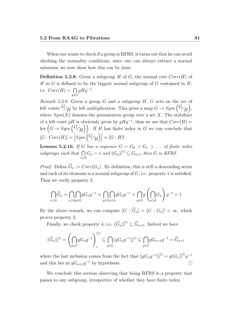
5.2 From RAAG to Fibrations 81
When one wants to check if a group is RFRS, it turns out that he can avoid
checking the normality conditions, since one can always extract a normal
subseries; we now show how this can be done.
Definition 5.2.8. Given a subgroup H of G, the normal core Core(H) of
H in G is defined to be the biggest normal subgroup of G contained in H,
i.e. Core(H) =⋂g∈G
gHg−1.
Remark 5.2.9. Given a group G and a subgroup H, G acts on the set of
left cosets G�H by left multiplication. This gives a map G→ Sym(G�H
),
where Sym(X) denotes the permutation group over a set X. The stabilizer
of a left coset gH is obviously given by gHg−1, thus we see that Core(H) =
ker(G→ Sym
(G�H
)). If H has finite index in G we can conclude that
[G : Core(H)] =∣∣∣Sym(G�H)∣∣∣ = [G : H]!.
Lemma 5.2.10. If G has a sequence G = G0 ⊃ G1 ⊃ . . . of finite index
subgroups such that⋂n≥0
Gn = 1 and (Gn)(1)r ⊆ Gn+1 then G is RFRS.
Proof. Define Gn := Core(Gn). By definition, this is still a descending series
and each of its elements is a normal subgroup of G, i.e. property 1 is satisfied.
Then we verify property 2
⋂n≥0
Gn =⋂n≥0
⋂g∈G
gGng−1 =
⋂g∈G
⋂n≥0
gGng−1 =
⋂g∈G
g
(⋂n≥0
Gn
)g−1 = 1
By the above remark, we can compute [G : Gn] = [G : Gn]! < ∞, which
proves property 3.
Finally, we check property 4, i.e. (Gn)(1)r ⊆ Gn+1. Indeed we have
(Gn)(1)r =
(⋂g∈G
gGng−1
)(1)
r
⊆⋂g∈G
(gGng−1)(1)
r ⊆⋂g∈G
gGn+1g−1 = Gn+1
where the last inclusion comes from the fact that (gGng−1)
(1)r = g(Gn)
(1)r g−1
and this lies in gGn+1g−1 by hypothesis.
We conclude this section observing that being RFRS is a property that
passes to any subgroup, irrespective of whether they have finite index.

82 5. Virtual Fibration of Hyperbolic 3-manifolds
Lemma 5.2.11. Let G be RFRS and H a subgroup; then H is RFRS.
Proof. Let {Gn} be a descending series of subgroups of G as in Definition
5.2.6 and let Hn := H ∩ Gn; then {Hn} is a descending series of subgroups
of H. Properties 1 and 2 are immediately verified. Then we observe that we
have a map H → G→ G�Gnwhose kernel is given by H∩Gn = Hn, therefore
we get an injection H�Hn↪→ G�Gn
into a group which is finite since Gn has
finite index in G by definition; this implies that Hn has finite index in H, i.e.
property 3. Finally we have that Hn ⊆ Gn implies that (Hn)(1)r ⊆ (Gn)
(1)r and
this sits in Gn+1 by hypothesis, therefore (Hn)(1)r ⊆ Hn+1 and 4 is proved.
5.2.2 Right-Angled Coxeter Groups
We now introduce a class of groups which is strictly connected to RAAGs,
which where introduced in section 3.3.1.
Definition 5.2.12. Let Γ be a simplicial graph. The right-angled Coxeter
group (RACG in the following) associated to Γ is the group with the following
presentation:
C(Γ) = 〈xi ∈ Γ0 | x2i ∀ xi ∈ Γ0 , [xi, xj] if {xi, xj} ∈ Γ1〉
This can be obviously obtained as the quotient of the RAAG A(Γ) on
the same graph by the normal subgroup generated by the squares of the
generators. RACGs (which are an example of the general class of Coxeter
groups) have been intensively studied since the beginning of the last century,
because they have many connection with reflection groups and the theory of
semisimple Lie algebras. Therefore it is quite interesting that RAAGs can be
embedded as subgroups of suitable RACGs: one hopes that in this way some
of the well-established properties of RACGs can be inferred for RAAGs as
well. This is actually the case for the RFRS condition, and this is what we
want to describe in this section.
First of all we show how to embed a RAAG in a RACG. The basic con-
struction is given by this example.
Example 5.2.13. Let Γ be the discrete graph on 2 points. Then C(Γ) =
Z2 ∗ Z2 = Dih∞ is the infinite dihedral group. This group can be concretely
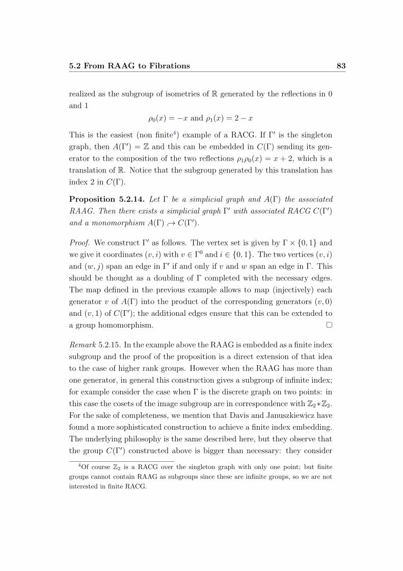
5.2 From RAAG to Fibrations 83
realized as the subgroup of isometries of R generated by the reflections in 0
and 1
ρ0(x) = −x and ρ1(x) = 2− x
This is the easiest (non finite4) example of a RACG. If Γ′ is the singleton
graph, then A(Γ′) = Z and this can be embedded in C(Γ) sending its gen-
erator to the composition of the two reflections ρ1ρ0(x) = x + 2, which is a
translation of R. Notice that the subgroup generated by this translation has
index 2 in C(Γ).
Proposition 5.2.14. Let Γ be a simplicial graph and A(Γ) the associated
RAAG. Then there exists a simplicial graph Γ′ with associated RACG C(Γ′)
and a monomorphism A(Γ) ↪→ C(Γ′).
Proof. We construct Γ′ as follows. The vertex set is given by Γ× {0, 1} and
we give it coordinates (v, i) with v ∈ Γ0 and i ∈ {0, 1}. The two vertices (v, i)
and (w, j) span an edge in Γ′ if and only if v and w span an edge in Γ. This
should be thought as a doubling of Γ completed with the necessary edges.
The map defined in the previous example allows to map (injectively) each
generator v of A(Γ) into the product of the corresponding generators (v, 0)
and (v, 1) of C(Γ′); the additional edges ensure that this can be extended to
a group homomorphism.
Remark 5.2.15. In the example above the RAAG is embedded as a finite index
subgroup and the proof of the proposition is a direct extension of that idea
to the case of higher rank groups. However when the RAAG has more than
one generator, in general this construction gives a subgroup of infinite index;
for example consider the case when Γ is the discrete graph on two points: in
this case the cosets of the image subgroup are in correspondence with Z2∗Z2.
For the sake of completeness, we mention that Davis and Januszkiewicz have
found a more sophisticated construction to achieve a finite index embedding.
The underlying philosophy is the same described here, but they observe that
the group C(Γ′) constructed above is bigger than necessary: they consider
4Of course Z2 is a RACG over the singleton graph with only one point; but finite
groups cannot contain RAAG as subgroups since these are infinite groups, so we are not
interested in finite RACG.
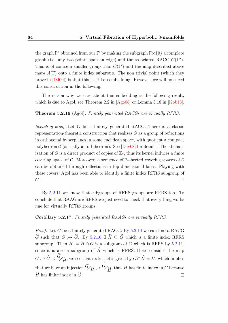
84 5. Virtual Fibration of Hyperbolic 3-manifolds
the graph Γ′′ obtained from our Γ′ by making the subgraph Γ×{0} a complete
graph (i.e. any two points span an edge) and the associated RACG C(Γ′′).
This is of course a smaller group than C(Γ′) and the map described above
maps A(Γ) onto a finite index subgroup. The non trivial point (which they
prove in [DJ00]) is that this is still an embedding. However, we will not need
this construction in the following.
The reason why we care about this embedding is the following result,
which is due to Agol, see Theorem 2.2 in [Ago08] or Lemma 5.18 in [Kob13].
Theorem 5.2.16 (Agol). Finitely generated RACGs are virtually RFRS.
Sketch of proof. Let G be a finitely generated RACG. There is a classic
representation-theoretic construction that realizes G as a group of reflections
in orthogonal hyperplanes in some euclidean space, with quotient a compact
polyhedron C (actually an orbihedron). See [Dav08] for details. The abelian-
ization of G is a direct product of copies of Z2, thus its kernel induces a finite
covering space of C. Moreover, a sequence of 2-sheeted covering spaces of Ccan be obtained through reflections in top dimensional faces. Playing with
these covers, Agol has been able to identify a finite index RFRS subgroup of
G.
By 5.2.11 we know that subgroups of RFRS groups are RFRS too. To
conclude that RAAG are RFRS we just need to check that everything works
fine for virtually RFRS groups.
Corollary 5.2.17. Finitely generated RAAGs are virtually RFRS.
Proof. Let G be a finitely generated RACG. By 5.2.14 we can find a RACG
G such that G ↪→ G. By 5.2.16 ∃ H ⊆ G which is a finite index RFRS
subgroup. Then H := H ∩ G is a subgroup of G which is RFRS by 5.2.11,
since it is also a subgroup of H which is RFRS. If we consider the map
G ↪→ G→ G�H, we see that its kernel is given by G∩ H = H, which implies
that we have an injection G�H ↪→ G�H, thus H has finite index in G because
H has finite index in G.

5.2 From RAAG to Fibrations 85
We already know that the fundamental group of a hyperbolic 3-manifold
is virtually embedded in a RAAG. By this theorem it is also virtually RFRS.
Then the strategy now is to show that a manifold with RFRS fundamental
group can be cut and covered in a suitable way, so that at each step we
have some kind of measure of how far the different pieces are from being
fibered. In the next paragraph we introduce the basic machinery involved in
this approach.
5.2.3 Thurston’s Norm on Homology
Now we describe a norm on the homology with real coefficients of a 3-
manifold introduced by Thurston in [Thu86]. This is based on a notion of
complexity for surfaces and turns out to be a powerful tool in the study
of fibrations of 3-manifolds. Beyond Thurston’s original paper, the topics
discussed here are treated in [Cal07] and [CaC00].
Definition 5.2.18. For a compact, connected and orientable surface S we
define the complexity of S as χ−(S) := max{−χ(S), 0}. For a disconnected
surface this is naturally defined as
χ−(S) :=n∑i=1
χ−(Si)
where the surfaces Si are the connected components of S.
We want to carry this notion from surfaces to homology classes in our
3-manifolds. To do this we need the following lemma. As always, let M be
a compact, connected and orientable 3-manifold, and let H∗ denote singular
homology with integer coefficients.
Lemma 5.2.19. Every class in H2(M,∂M) may be represented by a compact,
orientable and properly embedded surface.
Proof. By Lefschetz Duality we have H2(M,∂M) ∼= H1(M) and we recall
from 2.1.19 the identifications H1(M) = 〈M,S1〉. Therefore every class
σ ∈ H2(M,∂M) determines a map M → S1 unique up to homotopy; this
allows us to deform it to a smooth function. Then the preimage of a regular
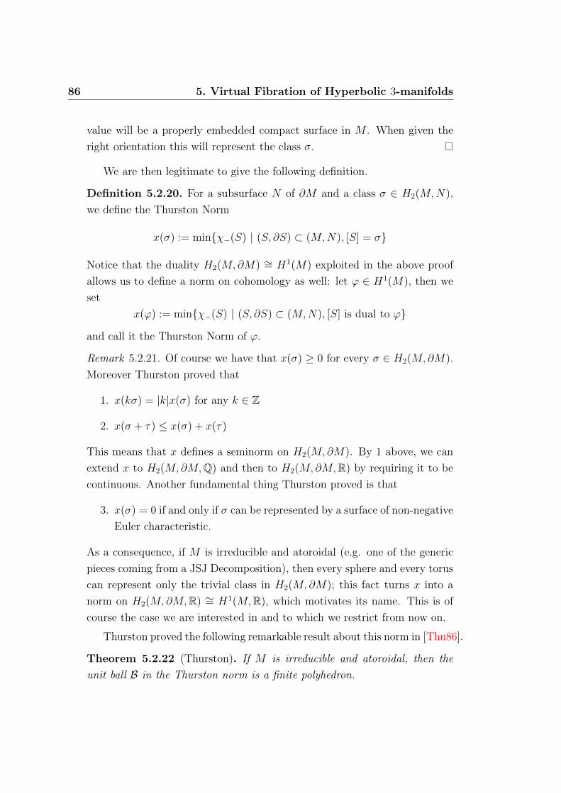
86 5. Virtual Fibration of Hyperbolic 3-manifolds
value will be a properly embedded compact surface in M . When given the
right orientation this will represent the class σ.
We are then legitimate to give the following definition.
Definition 5.2.20. For a subsurface N of ∂M and a class σ ∈ H2(M,N),
we define the Thurston Norm
x(σ) := min{χ−(S) | (S, ∂S) ⊂ (M,N), [S] = σ}
Notice that the duality H2(M,∂M) ∼= H1(M) exploited in the above proof
allows us to define a norm on cohomology as well: let ϕ ∈ H1(M), then we
set
x(ϕ) := min{χ−(S) | (S, ∂S) ⊂ (M,N), [S] is dual to ϕ}
and call it the Thurston Norm of ϕ.
Remark 5.2.21. Of course we have that x(σ) ≥ 0 for every σ ∈ H2(M,∂M).
Moreover Thurston proved that
1. x(kσ) = |k|x(σ) for any k ∈ Z
2. x(σ + τ) ≤ x(σ) + x(τ)
This means that x defines a seminorm on H2(M,∂M). By 1 above, we can
extend x to H2(M,∂M,Q) and then to H2(M,∂M,R) by requiring it to be
continuous. Another fundamental thing Thurston proved is that
3. x(σ) = 0 if and only if σ can be represented by a surface of non-negative
Euler characteristic.
As a consequence, if M is irreducible and atoroidal (e.g. one of the generic
pieces coming from a JSJ Decomposition), then every sphere and every torus
can represent only the trivial class in H2(M,∂M); this fact turns x into a
norm on H2(M,∂M,R) ∼= H1(M,R), which motivates its name. This is of
course the case we are interested in and to which we restrict from now on.
Thurston proved the following remarkable result about this norm in [Thu86].
Theorem 5.2.22 (Thurston). If M is irreducible and atoroidal, then the
unit ball B in the Thurston norm is a finite polyhedron.

5.2 From RAAG to Fibrations 87
This is interesting because this allows for a very nice characterization of
(co)homology classes associated to fibrations.
Remark 5.2.23. Let p : M → S1 be a fibration, i.e. the projection of a surface
bundle structure on M ; then it induces p∗ : π1(M)→ Z; by the identification
H1(X)←→ 〈X,S1〉 ←→ Hom(π1(X),Z)
of 2.1.19, we get a class in H2(M,∂M) ∼= H1(M).
Definition 5.2.24. A class in H2(M,∂M,Q) ∼= H1(M,Q) is called a fibered
class if it has some multiple induced by a fibration p : M → S1.
Notice that by definition if a class is fibered than any rational multiple
is again fibered. Therefore one can speak of a fibered ray. To state the
promised characterization we need some additional definitions.
Definition 5.2.25. Let F ⊂ B be a face of the Thurston unit ball in
H1(M,Q). The Thurston cone over F is the set {λf |f ∈ F, λ > 0}. In the
general case in which M is not irreducible atoroidal we define a Thurston cone
to be either one of these cones or a maximal connected subset of H1(M,Q)
on which x vanishes.
We then have this result of Thurston (see also Theorem 5.15 in [Cal07]).
Theorem 5.2.26 (Thurston). There exists a (possibly empty) collection
of open top-dimensional faces of the Thurston unit ball in H1(M,Q) such
that the fibered classes in H1(M,Q) are exactly the points contained in the
Thurston cones over the faces in this collection.
If the collection in the above statement is not empty, than the faces in
it are called fibered faces and the cones over them are called fibered cones.
This is justified by the fact that if a class sits on a top dimensional face of
the Thurston ball in H1(M,Q) and is fibered, then every other class on the
same face is also fibered and any of its multiples is fibered too.
5.2.4 Virtual Fibration of RFRS Manifolds
In [Ago08] Agol proves the following result.
88 5. Virtual Fibration of Hyperbolic 3-manifolds
Theorem 5.2.27 (Agol). Let M be a compact irreducible orientable 3-manifold
with χ(M) = 0. If π1(M) is RFRS then M virtually fibers over the circle.
The idea of Agol’s proof is this: suppose S ⊂ M is an oriented surface
which is non-separating, i.e. M \ \S is connected. Then S is the fiber of a
fibration over S1 if and only if M \ \S ∼= S × I. Otherwise M \ \S admits
a non trivial JSJ Decomposition in which we find some pieces which are the
product of a surface and an interval and pieces which are not products of
this kind. Agol’s RFRS condition allows to pass to suitable covers of M in
which these non-product pieces are somehow “killed”.
We can find in the literature (at least) two approaches to this idea. The
first is Agol’s original paper ([Ago08]), where he uses the theory of least-
weight taut normal surfaces, which has a strong combinatorial flavour; the
second is due to a later paper of Friedl and Kitayama ([FrK12]) and exploits
the properties of sutured manifolds. In this section we give a precise meaning
to the above idea and describe the main steps of the construction, focusing
on the role of the RFRS condition.
Definition 5.2.28. A sutured manifold is a 3-manifold M with a decom-
position of its boundary into oriented submanifolds ∂M = R− ∪ γ ∪ R+,
where
• γ is a disjoint union of annuli (the sutures),
• R− and R+ are disjoint subsurfaces of ∂M such that for each component
A of γ we have that A ∩R− is a boundary of both A and R−, and the
same for R+,
• R− and R+ are oriented so that they induce the same orientation on
each component of γ.
When the above conditions are satisfied we also say that (M,R−, R+, γ) is a
sutured manifold.
The most basic (but nevertheless central) examples are the following.
Example 5.2.29. Let S be a surface and let M = S × I. Then
(M,S × {−1}, S × {1}, ∂S × I)
5.2 From RAAG to Fibrations 89
is a sutured manifold when things are endowed with the obvious orientations.
We call such a manifold a product sutured manifold.
Example 5.2.30. Let M be a closed 3-manifold and S ⊂ M a properly
embedded surface. Then we get an associated sutured manifold
M(S) := (M \ (S × I), S × {−1}, S × {1},∅)
We explicitly observe that S is the fiber of a fibration over the circle if and
only if M(S) is product sutured manifold.
The last example can be generalized to the case of non empty boundary
by taking care of the boundary data. The idea is that if we choose the surface
nice enough (with respect to the boundary) then M \ \S will be endowed
with a canonical structure of sutured manifold and we say that it is a sutured
manifold obtained by sutured decomposition along S; then the theory goes
on mimicking the theory of Haken manifolds and constructing a so-called
sutured hierarchy. More details can be found in [Sch90] and [FrK12]. We are
especially interested in Theorem 3.2 of [FrK12], which can roughly be stated
as follows.
Theorem 5.2.31. Let (M,R−, R+, γ) be an irreducible sutured manifold.
Then there exists a product sutured submanifold P ⊆ M , unique up to iso-
topy, such that any other product submanifold can be isotoped into P .
In other words this means that a sutured manifold structure on a 3-
manifold gives rise to a “maximal product core”, essentially unique. This
justifies the intuition behind the following definition (and also proves that it
is well posed).
Definition 5.2.32. Let (M,R−, R+, γ) be an irreducible sutured manifold
and let P the product sutured submanifold of the previous theorem. We call
a window of M any component of P and a gut any component of M \ \P .
The guts of M are the pieces we are left with after removing the product
part of it. They carry non trivial topological information and are an ob-
struction to M being a surface bundle over the circle. The point of Agol’s
work is that there are suitable covering manifolds where these pieces can
be simplified; these coverings are indeed chosen among those induced by a
90 5. Virtual Fibration of Hyperbolic 3-manifolds
RFRS series for the fundamental group. The Thurston norm is used in this
procedure in order to choose the appropriate surfaces to cut along and to
detect fibered classes (in the light of Theorem 5.2.26). This is Agol’s original
statement.
Theorem 5.2.33 (Agol). Let M be connected orientable irreducible 3-manifold
with χ(M) = 0 and π1(M) RFRS. If f ∈ H1(M) is a non trivial and non
fibered class then there is a finite cover p : N → M such that p∗f ∈ H1(N)
sits in the cone over the boundary of a fibered face of the Thurston ball B of
N .
The proof is quite technical and we refer the reader to the original paper
of Agol [Ago08], or [FrK12] for a more detailed exposition. We just say a few
words to give some ideas of why the purely algebraic RFRS condition should
have something to do with this geometric procedure of cutting and covering.
The RFRS condition consists of two parts:
• residual finiteness, which is related to the problem of embedding im-
mersed compact subsets into suitable covering spaces,
• rational solvability, which has something to say about “homological
largeness” of covering spaces.
We begin with the first one.
Definition 5.2.34. A group G is residually finite if ∀ g ∈ G, g 6= 1 there is
H ≤ G of finite index such that g 6∈ H.
The interest of this definition lies in the following result (see Lemma 1.3
in Scott’s paper [Sco78]).
Lemma 5.2.35. Let X be a Hausdorff topological space with regular covering
space X and covering group G. Then G is residually finite if and only if for
every compact subset K ⊂ X we can find an intermediate finite covering
space X → X ′ → X such that C projects homeomorphically onto X ′.
The property of being residually finite is equivalent to saying that the
intersection of all the finite index subgroups of G is trivial; therefore we see
that a RFRS group is in particular residually finite. For the applications

5.2 From RAAG to Fibrations 91
in 3-manifold topology we are especially interested in the case K is either a
compact subsurface of our manifold, for example one of the immersed surfaces
obtained by Kahn and Markovic, or some of the guts components induced
by a sutured manifold structure.
Finally we turn to the rational solvability part and the usefulness of work-
ing with rational coefficients.
Definition 5.2.36. Let p : X → X a covering projection of degree n. We
define a map at the level of singular chains over any PID R as follows. Let
σ : ∆k → X be a singular k-simplex and let {σ1, . . . , σn} be its lifting to X.
Define the so-called transfer homomorphism as
t : Ck(X,R)→ Ck(X, R), σ →n∑i=1
σi
It is clear that composing the transfer map with the covering projection
gives a map from Ck(X,R) onto itself which is just multiplication by n =
deg(p). Moreover the transfer map commutes with the boundary operator,
therefore we get a pair of maps in homology (which we still call p and t)
Hk(X,R)t→ Hk(X, R)
p→ Hk(X,R)
whose composition pt : Hk(X,R)→ Hk(X,R) is just multiplication by n on
Hk(X,R). As a result we have that ker(pt) consists of torsion elements in
Hk(X,R) whose order divides n.
Remark 5.2.37. Working with coefficients in R = Q is just the same as
working with integral homology modulo torsion; this implies that if we have
a finite covering p : X → X then the above map pt : Hk(X,Q)→ Hk(X,Q)
is injective, just because Q-homology groups are torsion free. But then also
t : Hk(X,Q) → Hk(X,Q) in necessarily injective. This can informally be
stated saying that the rational homology of X is larger than that of X. By
duality the same holds for cohomology.
We apply this machinery in the case X is a closed hyperbolic 3-manifold
M which has a decomposition into windows and guts as described above.
Quoting Agol’s original paper:

92 5. Virtual Fibration of Hyperbolic 3-manifolds
The idea is to produce a complexity of the guts, and use the
RFRS condition to produce a cover of M to which a component
of the guts lifts and for which we can decrease the complexity
of the guts, by “killing” it using non-separating surfaces coming
from new homology in this cover.
The complexity Agol refers to is (a slightly modified version of) an invariant
introduced by Gabai in [Gab83] which is defined for sutured manifolds and
takes its values in a linearly ordered set in which strictly descending chains
are finite. This means that if we are able to iteratively find finite covers
where this complexity drops then in the end we are left with no guts, that is
we have found a finite cover which is a surface bundle.
Bibliography
[Ago08] I. Agol. Criteria for Virtual Fibering, preprint arXiv:
math/0707.4522 [math.GT], 2008.
[Ago12] I. Agol. The Virtual Haken Conjecture, preprint arXiv:
math/1204.2810 [math.GT], 2012.
[AFW12] M. Aschenbrenner, S. Friedl, H. Wilton. 3-manifold Groups,
preprint arXiv: math/1205.0202 [math.GT], 2012.
[BP92] R. Benedetti, C. Petronio. Lectures on Hyperbolic Geometry,
Springer, Berlin, 1992.
[BW10] N. Bergeron, D. Wise. A Boundary Criterion for Cubulation,
preprint arXiv: math/0908.3609v3 [math.GT], 2010.
[Bon02] F. Bonahon. Geometric Structure on 3-Manifolds, Handbook of Geo-
metric Topology (R. Daverman, R. Sher eds.), Elsevier, 93-164, 2002.
[BrH99] M.R. Bridson. Metric Spaces of Non-Positive Curvature, Springer,
Berlin, 1999.
[Cal07] D. Calegari. Foliations and the Geometry of 3-Manifolds, Oxford
University Press, Oxford, 2007.
[CaC00] A. Candel, L. Conlon. Foliations, American Mathematical Society,
Providence, 2000.
[Cha06] R. Charney. An Introduction to Right-angled Arting Groups,
preprint arXiv: math/0610668v1 [math.GR], 2006.
93
94 BIBLIOGRAPHY
[Dav08] M.W. Davis. The Geometry and Topology of Coxeter Groups,
Princeton University Press, Princeton, 2008.
[DJ00] M.W. Davis, T. Januszkiewicz. Right-angled Artin Groups are com-
mensurable with Right-angled Coxeter Groups, Journal of Pure and Ap-
plied Algebra, 153, 229-235, 2000.
[FrK12] S. Friedl, T. Kitayama. The Virtul Fibering Theorem for 3-
manifolds, preprint arXiv: math/1210.4799 [math.GT], 2012.
[Gab83] D. Gabai. Foliations and the Topology of 3-manifolds, Journal of
Differential Geometry 18, no. 3, 445-503, 1983.
[Gro87] M. Gromov. Hyperbolic Groups, Essays in Group Theory (S.M. Ger-
sten, ed), Springer, MSRI Publications 8, 75-263, 1987.
[HaW08] F. Haglund, D. Wise. Special Cube Complexes, Geometric and
Functional Analysis 17, no. 5, 1551-1620, 2008.
[Hat02] A. Hatcher. Algebraic Topology. Cambridge University Press, Cam-
bridge, 2002.
[Hat] A. Hatcher. Notes on Basic 3-Manifold Topology.
[Hem76] J. Hempel. 3-Manifolds, Annals of Mathematical Studies, vol. 86,
Princeton University Press, Princeton, 1976.
[HW99] T. Hsu, D. Wise. On Linear and Residual Properties of Graph Pro-
ducts, Michigan Mathematical Journal, 46 (2), 251-259, 1999.
[Jac77] W. Jaco. Lectures on Three-Manifold Topology, CBMS Regional Con-
ference Series in Mathematics, no. 43, Providence, 1977.
[Hae91] A. Haefliger. Complexes of Groups and Orbihedra, Group Theory
from a Geometrical Viewpoint (Trieste, 1990), World Scientific Publi-
shing, River Edge, NJ, 504-540, 1991.
[KM09] J. Kahn, V. Markovic. Immersing Almost Geodesic Surfaces in a
Closed Hyperbolic Three Manifold, preprint arXiv: math/0910.5501v5
[math.GT], 2009.

BIBLIOGRAPHY 95
[KS77] R.C. Kirby, L.C. Siebenmann. Foundational Essays on Topological
Manifolds, Smoothings and Triangulations, Princeton University Press,
1977.
[Kob13] T. Koberda. Right-angled Artin Groups and their Subgroups, notes
for a course at Yale University, 2013.
[LyS77] R. Lyndon, P. Schupp. Combinatorial Group Theory, Springer,
Berlin, 1977.
[Sag95] M. Sageev. Ends of Group Pairs and Non-positively Curved Cube
Complexes, Proceedings of the London Mathematical Society (3), 71
(3), 585-617, 1995.
[Sag97] M. Sageev. Codimension-1 Subgroups and Splitting of Groups, Journ-
al of Algebra, 189 (2), 377-389, 1997.
[Sch90] M.G. Scharlemann. Lectures on the Theory of Sutured 3-manifolds,
Korea Advanced Institute of Technology Workshop Proceedings, 25-46,
1990.
[Sco78] P. Scott, Subgroups of Surface Groups are Almost Geometric, Journal
of the London Mathematical Society, Second Series 17, no. 3, 357-381,
1978.
[Sco83] P. Scott, The Geometries of 3-Manifolds, Bullettin of the London
Mathematical Society, 15, 401-487, 1983.
[Thu86] W. P. Thurston. A Norm for the Homology 3-manifolds. Memories
of the American Mathematical Society, 339, 99-130, 1986.
[Thu] W. P. Thurston. The Geometry and Topology of Three-manifolds.
[Thu82] W. P. Thurston. Three Dimensional Manifolds, Kleinian Groups
and Hyperbolic Geometry, Bullettin of the American Mathematical So-
ciety, vol. 6, no. 3, 1982.
[Wil02] H. Wilton. The 3-dimensional Geometrisation Conjecture of W.P.
Thurston, online notes, 2002.

96 BIBLIOGRAPHY
[Wi12] D. Wise. From Riches to Raags: 3-Manifolds, Right-Angled Artin
Groups, and Cubical Geometry, CBMS Regional Conference Series in
Mathematics, no. 117, Providence, 2012.
[Wi11] D. Wise. The Structure of Groups with a Quasiconvex Hierarchy,
preprint, 2011.

Acknowledgements
I want to thank my advisor, Stefano Francaviglia, for the enthusiasm,
the patience, the trust and the encouragement he has shown me during the
preparation of this thesis. I also want to thank Rita Fioresi and Luca Mi-
gliorini for all the time and energy they have spent in teaching me geometry
and algebra, both inside and outside the teaching hours. A special thanks
also goes to Alberto Parmeggiani for his guidance and his precious advices
throughout my studies.
I also want to thank the institutions that have given me some kind of
financial support during these years, as AILA, the Departments of Mathe-
matics of Bologna and Pisa and the Collegio Superiore of Bologna.